numerical analysis of fluid flow and heat transfer...

Fluid Mechanics 2018; 4(1): 1-13

http://www.sciencepublishinggroup.com/j/fm

doi: 10.11648/j.fm.20180401.11

ISSN: 2575-1808 (Print); ISSN: 2575-1816 (Online)

Numerical Analysis of Fluid Flow and Heat Transfer Based on the Cylindrical Coordinate System

Mohammad Hassan Mohammadi

Institute of Mathematics, Department of Differential Equations, National Academy of Sciences of Armenia, Marshal Baghramyan Av.,

Yerevan, Armenia

Email address: [email protected]

To cite this article: Mohammad Hassan Mohammadi. Numerical Analysis of Fluid Flow and Heat Transfer Based on the Cylindrical Coordinate System. Fluid

Mechanics. Vol. 4, No. 1, 2018, pp. 1-13. doi: 10.11648/j.fm.20180401.11

Received: October 18, 2017; Accepted: December 8, 2017; Published: January 15, 2018

Abstract: In this work we will apply the three-dimensional mathematical modelling of fluid flow and heat transfer inside the

furnaces based on the cylindrical coordinate system to describe the behavior of the transport phenomena. This modelling is

constructed by using the mass, momentum, and energy conservation laws to achieve the continuity equation, the Navier-Stokes

equations, and the energy conservation equation. Due to the moving boundary between the solid and melted materials inside of

the furnaces we will impose the Stefan condition to describe the behavior of the free boundary between two phases. We will

derive the variational formulation of the system of transport phenomena, then we will discrete the domain to complete the

finite element method stages and we will obtain the system of nonlinear equations in 256 equations in 256 unknowns. To get

the numerical solution of the large-scale system we will prepare a convenient mathematical work and gain some diagrams

where they would be applicable in the design process of the furnaces shapes.

Keywords: Fluid Flow, Heat Transfer, Mathematical Modeling, Stefan Condition, Cylindrical Coordinate

1. Introduction

Mathematical modeling of heat transfer is applied to

investigate the environment of the furnaces and transport

phenomena inside them, because it has the advantages of low

cost and acceptable exactness. Quan-Sheng and You-Lan

consider the two-dimensional Stefan problem in (1985) and

they used the singularity-separating method to prepare the

numerical solution. Ungan and Viskanta in (1986), (1987)

investigated modeling of circulation and heat transfer in a

glass melting tank in three-dimension. Henry and Stavros in

(1996) prepared the convenient work about the mathematical

modelling of solidification and melting process. Vuik, Segal,

and Vermolen in (2000) studied about the discretization

approach for a Stefan problem where they focused on

interface reaction at the free boundary.

Pilon, Zhao, and Viskanta in (2002), (2006) in their papers

considered three-dimensional flow and researched about the

behavior of thermal structures in glass melting furnaces by

using the three-dimensional mathematical modeling. Their

works were included theoretical and numerical sections

where they applied sufficient boundary conditions. Sadov,

Shivakumar, Firsov, Lui, and Thulasiram, provided an article

about the mathematical model of ice melting on transmission

lines in (2007). Choudhary, Venuturumilli, and Matthew in

(2010) in their common paper introduce the mathematical

modeling of flow and heat transfer phenomena in glass

melting where it consists of delivery and forming processes,

especially the turbulent conditions has been discussed in the

paper for Newtonian and non-Newtonian fluids.

Kambourova, and Zheleva had modelized and described

temperature distributions ina tank of glass melting furnace in

(2002).

The author studied the mathematical modeling of heat

transfer and transport phenomena in (2016) in two-dimension

with Stefan free boundary based on stream functions. due to

the advantages of stream functions mathematical modeling

has prepared and by invoking the finite element method the

numerical solution of the transport phenomena derived, also

we did the same work in three-dimension. In the current

work we will apply the mathematical modeling in three-

dimension for the especial furnaces with cylindrical shapes,

that they are called Garnissage tank. Due to their shapes we

will illustrate the mathematical equations of transport

2 Mohammad Hassan Mohammadi: Numerical Analysis of Fluid Flow and Heat Transfer

Based on the Cylindrical Coordinate System

phenomena in the cylindrical coordinate system in three-

dimension to use its symmetric properties.

The melting process in the Garnissage furnace starts when

we impose the heat to the solid material by electrical boosters

inside it, but the heat transferring by electrical boosters

couldn’t melt the whole materials and whenever the central

parts are melted the parts far from the boosters is solid. In

this case the boundary between the solid and liquid materials

are moving during the process, then we will have free

boundary problem. The Stefan condition is sufficient tool to

describe the behavior of the free boundary and we will

handle three-dimensional version of the Stefan condition in

the mathematical modeling process.

We state the conservation equations in the cylindrical

coordinate, so the Stefan condition, then we convert the

system of equations into the weak formulation. For

expressing the system in the variational formulation we will

use convenient test functions with small support and then we

will discrete the domain to follow the finite element method.

The approximate values of the variables would be applied

instead of the variables, and finally we will get the system of

equations that they are combination of linear and nonlinear

equations, thus to solve the system numerically the Newton’s

method would be recommended.

2. Mathematical Modeling

We start the paper by reviewing the mathematical

modeling of fluid flow in three-dimension. Cylindrical

coordinate is applied for modeling because it provides the

convenient environment to express the modeling, hence we

can use the symmetric properties to introduce the equations.

There are three different parts in the modeling process which

we will introduce them.

2.1. Continuity Equation

+ = 0 (1)

2.2. Navier-Stokes Equations

+ + = − + + − + (2)

+ + = − + + + (3)

2.3. Energy Equation

+ + = + + (4)

Deriving the weak formulation is second stage of the work after the mathematical modeling, then the variational version of

the modeling has been obtained by imposing the convenient smooth test function with small support and using the integration

by parts technique. Like the classical modeling the variational formulation has three sections:

2.4. Continuity Equation (Weak Formulation)

− − = 0 (5)

2.5. Navier-Stokes Equations (Weak Formulation)

+ ! + + + − − = − " − (6)

+ + + ! + + = − " − (7)

2.6. Energy Equation (Weak Formulation)

# $ + + + + + % + # + & = − (8)

3. Discretization of Domain

After weak formulation we discrete the domain Ω , and

replace the approximate variables (, (, "(, and #( in the

variational formulation to obtain the algebraic system of

equations. Assume that *( ⊂ ,-Ω, which consists of test

functions that they are piecewise continuous with the fix

degree, and also suppose that

dim*( = 2ℎ, *( = 4"5678, 8!, 89, … , 8;(<,

where the basis functions 8=, >, ?, @, A = 1,2, … , 2ℎ ,

have small support. If we choose the finite dimensional

subspace *(, and also the correspond variables in *(, then we

redefine the heat transfer problem as the problem of finding (, (, "( , and #( such that there satisfy in the equations

Fluid Mechanics 2018; 4(1): 1-13 3

(5), (6), (7), and (8). Now we define the approximate

solutions (, ( , "(, and #( in terms of the basis functions 8=, >, ?, @ (, >, ?, @ = ∑ E=8=, >, ?, @;(=F , (9)

(, >, ?, @ = ∑ E =8=, >, ?, @;(=F , (10)

"(, >, ?, @ = ∑ G=8=, >, ?, @;(=F , (11)

#(, >, ?, @ = ∑ #=8=, >, ?, @;(=F , (12)

where E= , E = , G= , #= , A = 1,2,3, … , 2ℎ , must be

determined. We insert the values of (, ( , "( , #( ∈ *(

instead of , , ", #in the variational formulation of the heat

transfer problem. In this case the heat transfer problem is

restated as the problem of finding

UKL , UK , … , UKMN ∈ RPQ, URL , UR , … , URMN ∈ RPQ, Sθ, θ!, … , θPQU ∈ RPQ,

where they are satisfied in the system of equations

∑ SE=5= − E =V=U;(=F = 0, (13)

∑ E=W=;(=F + ∑ ∑ E=EXY=X;(XF;(=F +∑ ∑ E=E X;(XF Z=X;(=F + ∑ G=[=;(=F + \ = 0, (14)

∑ E =W]=;(=F + ∑ ∑ E =E XY]=X;(XF;(=F +∑ ∑ E =EXZ]=X;(XF;(=F + ∑ G=[]=;(=F + \] = 0, (15)

∑ #= =;(=F +∑ ∑ #= EX + E X _X;(XF;(=F +, = 0, (16)

` = 1,2,3, … , 2ℎ, which coefficients of the system are defined as

Table 1. System Coefficients.

5= = a 8= b8 − c8c d V= = a 8= c8c?

W= = a 8= $c8c@ − c!8c! − c

!8c?! + 1 c8c % W]= = a 8= $c8c@ + c

!8cc? + c!8c?! %

Y=X = 12a 8=8X c8c Y]=X = 12a 8=8X c8c?

Z=X = a 8= $8X c8c? + 8 c8Xc? % Z]=X = a 8= $8X c8c + 8 c8Xc %

[= = 1 a 8= c8c []= = 1 a 8= c8c?

\ = a 8 \] = a 8

= = a 8= ec8c@ + f $c!8c! + c

!8c?! %g _X = a $8 c8Xc + 8X c8c %

, = 1f a b`h c8c@ + 8d

We need to determine the values of the coefficients to derive the numerical solution of system, then we must define the

sufficient domain and discrete it to compute the relevant integrals, and at last we would found all coefficients and finally we

will earn the numerical solution of the system for the interpretation of the fluid behavior in the furnaces.

4. Unknown Coefficients

We continue the process by computing the coefficients in the transport system, for this objective we need to divide the

domain Ω to the mesh cubes, the Figure 1 shows the Ai` −mesh cube where we will construct the test functions on Ai` −mesh

cube.



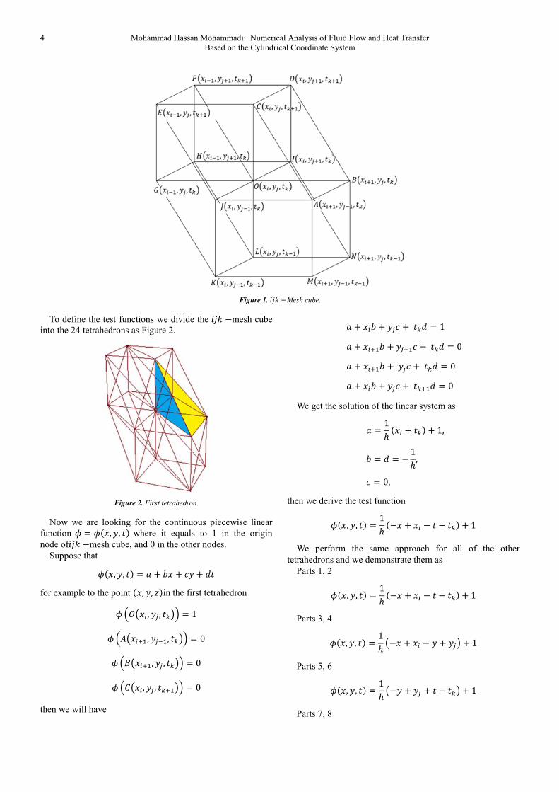
Figure 1. Ai` −Mesh cube.

To define the test functions we divide the Ai` −mesh cube

into the 24 tetrahedrons as Figure 2.

Figure 2. First tetrahedron.

Now we are looking for the continuous piecewise linear

function 8 = 8j, k, @ where it equals to 1 in the origin

node ofAi` mesh cube, and 0 in the other nodes.

Suppose that

8j, k, @ 5 Vj fk l@ for example to the point j, k, ?in the first tetrahedron

8 mSj= , kX , @U 1

8 WSj=n, kXo, @U 0

8 YSj=n, kX , @U 0

8 ZSj= , kX , @nU 0

then we will have

5 j=V kXf @l 1

5 j=nV kXof @l 0

5 j=nV kXf @l 0

5 j=V kXf @nl 0

We get the solution of the linear system as

5 13 j= @ 1,

V l 13, f 0,

then we derive the test function

8j, k, @ 13 j j= @ @ 1

We perform the same approach for all of the other

tetrahedrons and we demonstrate them as

Parts 1, 2

8j, k, @ 13 j j= @ @ 1

Parts 3, 4

8j, k, @ 13 Sj j= k kXU 1

Parts 5, 6

8j, k, @ 13 Sk kX @ @U 1

Parts 7, 8


8j, k, @ = 1ℎ j − j= + @ − @ + 1

Parts 9, 10

8j, k, @ = 1ℎ Sj − j= + k − kXU + 1

Parts 11, 12

8j, k, @ = 1ℎ Sk − kX − @ + @U + 1

Parts 13, 14

8j, k, @ = 1ℎ −@ + @ + 1

Parts 15, 16

8j, k, @ = 1ℎ j − j= + 1

Parts 17, 18

8j, k, @ = 1ℎ S−k + kXU + 1

Parts 19, 20

8j, k, @ = 1ℎ @ − @ + 1

Parts 21, 22

8j, k, @ = 1ℎ Sk − kXU + 1

Parts 23, 24

8j, k, @ = 1ℎ −j + j= + 1

We are in the position to compute the coefficients of the

continuity equation 5= and V= for the system (13), then we

continue the process by determining the 5= for

` = A, ` = A − 2! + 2 − 1, ` = A + 2! + 2 − 1,

and it is trivial that 5= = 0 in the other cases. Then we

divide the integral as

5== = a 8= b8= − c8=c d

= q 8= b8= − c8=c d ll?l@rsKt-+ q 8= b8= − c8=c d ll?l@rsKt-!

+⋯+ q 8= b8= − c8=c d ll?l@rsKt!v.

We compute the values of integrals in different tetrahedrons separately and derive the final value of 5== as

j= + ℎ6j=! − 8j=j= + ℎ! + 3j= + ℎ96ℎ! ln b1 + ℎj=d − j=v − 4j=ℎ9 + 3ℎv6ℎ! ln b1 − ℎj=d − j=3j=

! + ℎ!9ℎ , and by the similar operation we gain

5=,=oS;n;oU = 172ℎ 12j=9 − 6j=!ℎ + 40j=ℎ! − 3ℎ9 − 16ℎ! j=v + 3j=!ℎ! + 2j=ℎ9 − 2ℎv ln b1 + ℎj=d, 5=,=nS;n;oU = 172ℎ 12j=9 + 6j=!ℎ + 40j=ℎ! + 3ℎ9 + 16ℎ! j=v + 3j=!ℎ! − 2j=ℎ9 − 2ℎv ln b1 − ℎj=d.

Also for the coefficient V=in (13) we get

V== = 0, V=,=oS;n;oU = − ℎ!12, V=,=nS;n;oU = ℎ!12.

Suppose that the domain

Ω = 0.3, 0.9 × 0.3, 0.9 × 0.3, 0.9, and 2 = 4, then ℎ = 0.15, and



j 0.3, j! = 0.45, j9 = 0.6, jv = 0.75, after inserting the values in the system (13) we will reach the coefficients matrix G, with 64 rows and 128 columns, where

G =

0.41 0 … 0 0.0009 0 0 0 ⋱ 0 0 0 0 00 0.62 0 … 0 0.0001 0 0 ⋱ 0 0 0 0 0⋮ 0 0.67 0 … 0 −0.0003 0 ⋱ 0 0 0 0 00 ⋮ 0 0.41 0 … 0 −0.0006 ⋱ 0 0 0 0 00.003 0 ⋮ 0 0.41 0 … 0 ⋱ 0 0 0 0 00 0.002 0 ⋮ 0 0.62 0 … ⋱ 0.0009 0 0 0 00 0 0.002 0 ⋮ 0 0.67 0 ⋱ 0 0.0001 0 0 00 0 0 0.002 0 ⋮ 0 0.41 ⋱ ⋮ 0 −0.0003 0 00 0 0 0 0.003 0 ⋮ 0 ⋱ 0 ⋮ 0 −0.0006 00 0 0 0 0 0.002 0 ⋮ ⋱ 0.41 0 ⋮ 0 0.00090 0 0 0 0 0 0.002 0 ⋱ 0 0.41 0 ⋮ 00 0 0 0 0 0 0 0.002 ⋱ 0 0 0.62 0 ⋮0 0 0 0 0 0 0 0 ⋱ 0 0 0 0.67 00 0 0 0 0 0 0 0 ⋱ 0.003 0 0 0 0.41

and

=

0 0 … 0 0.002 0 0 0 ⋱ 0 0 0 0 00 0 0 … 0 0.002 0 0 ⋱ 0 0 0 0 0⋮ 0 0 0 … 0 0.002 0 ⋱ 0 0 0 0 00 ⋮ 0 0 0 … 0 0.002 ⋱ 0 0 0 0 0−0.002 0 ⋮ 0 0 0 … 0 ⋱ 0 0 0 0 00 −0.002 0 ⋮ 0 0 0 … ⋱ 0.002 0 0 0 00 0 −0.002 0 ⋮ 0 0 0 ⋱ 0 0.002 0 0 00 0 0 −0.002 0 ⋮ 0 0 ⋱ ⋮ 0 0.002 0 00 0 0 0 −0.002 0 ⋮ 0 ⋱ 0 ⋮ 0 0.002 00 0 0 0 0 −0.002 0 ⋮ ⋱ 0 0 ⋮ 0 0.0020 0 0 0 0 0 −0.002 0 ⋱ 0 0 0 ⋮ 00 0 0 0 0 0 0 −0.002 ⋱ 0 0 0 0 ⋮0 0 0 0 0 0 0 0 ⋱ 0 0 0 0 00 0 0 0 0 0 0 0 ⋱ −0.002 0 0 0 0

Now we have obtained a linear system of equations that it has 128 variables EL , E , … , E; E L , E , … , E within 64

equations. We will return to the system (13) in the next sections again, thus we focus on the Navier-Stokes system (14) to earn

the remainder coefficients.

We continue the process by determining the coefficients of the Navier-Stokes system (14), (15). We start by specifying the

coefficient W= , and as we done before we suppose the Ai` −mesh cube that it was divided to 24 tetrahedrons, then after

integration process in the whole parts we gain

W== = − n(9( ln 1 + ( + o(9( ln 1 − ( + n!(( , (17)

W=,=oS;n;oU = − ( 6j=! + 15j=ℎ + 11ℎ! + n(9( ln 1 + ( − (!, (18)

W=,=nS;n;oU = − ( 6j=! − 15j=ℎ + 11ℎ! + o(9( ln 1 − ( + (!. (19)

Now we insert the values of W= from (17), (18), and (19) into the ∑ E=W=;(=F from (14) and we earn the coefficient matrix W=v×v as


0.008 0 … 0 0.004 0 0 0 ⋱ 0 0 0 0 00 0.003 0 … 0 0.002 0 0 ⋱ 0 0 0 0 0⋮ 0 0.002 0 … 0 0.001 0 ⋱ 0 0 0 0 00 ⋮ 0 0.001 0 … 0 0.0005 ⋱ 0 0 0 0 0−0.07 0 ⋮ 0 0.008 0 … 0 ⋱ 0 0 0 0 00 −0.33 0 ⋮ 0 0.003 0 … ⋱ 0.004 0 0 0 00 0 −0.78 0 ⋮ 0 0.002 0 ⋱ 0 0.002 0 0 00 0 0 −1.43 0 ⋮ 0 0.001 ⋱ ⋮ 0 0.001 0 00 0 0 0 −0.07 0 ⋮ 0 ⋱ 0 ⋮ 0 0.0005 00 0 0 0 0 −0.33 0 ⋮ ⋱ 0.001 0 ⋮ 0 0.0040 0 0 0 0 0 −0.78 0 ⋱ 0 0.008 0 ⋮ 00 0 0 0 0 0 0 −1.43 ⋱ 0 0 0.003 0 ⋮0 0 0 0 0 0 0 0 ⋱ 0 0 0 0.002 00 0 0 0 0 0 0 0 ⋱ −0.07 0 0 0 0.001

We continue the process of finding the coefficients of the Navier-Stokes system (14) by focusing on the coefficient Y=X

from ∑ ∑ E=EXY=X;(XF;(=F , and we achieve

Y=== = 0

Y=,=oS;n;oU,= = − ℎ!20

Y=,=nS;n;oU,= = ℎ!20

Y=,=oS;n;oU,=oS;n;oU = ℎ!20

Y=,=nS;n;oU,=nS;n;oU = − ℎ!20

Y=,=,=oS;n;oU = ℎ!60

Y=,=,=nS;n;oU = − ℎ!60

then by applying the values Y=X we will obtain the value of ∑ ∑ E=EXY=X;(XF;(=F as

for ` < 20

ℎ!10EESLU + ℎ!60EL!

for 20 ≤ ` ≤ 45

− ℎ!10EESLU + ℎ!10EESLU − ℎ

!60EL! + ℎ!60EL!

for ` > 45

− ℎ!10EESLU − ℎ!60EL!

Also the values of Z=X are as

Z=== = 0

Z=,=oS;n;oU,= = ℎ!15



Z=,=nS;n;oU,= = − ℎ!15

Z=,=,=oS;n;oU = ℎ!15

Z=,=,=nS;n;oU = − ℎ!15

Z=,=oS;n;oU,=oS;n;oU = −ℎ!5

Z=,=nS;n;oU,=nS;n;oU = ℎ!5

then we insert the values Z=X to get the ∑ ∑ E=E XZ=X;(XF;(=F as

for ` < 20

− ℎ!15EE SLU − ℎ!5 E ESLU + ℎ

!15ESLUE SLU

for 20 ≤ ` ≤ 45

− ℎ!15ESLUE SLU + ℎ!5 ESLUE + ℎ

!15EE SLU − ℎ

!15EE SLU − ℎ

!5 ESLUE

+ ℎ!15ESLUE SLU for ` > 45

ℎ!15EE SLU − ℎ!15ESLUE SLU + ℎ

!5 ESLUE

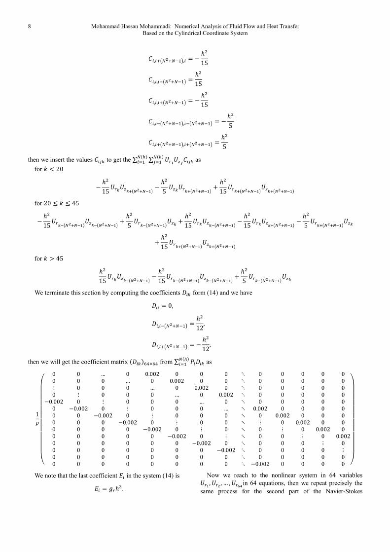
We terminate this section by computing the coefficients [= form (14) and we have

[== = 0, [=,=oS;n;oU = ℎ!12, [=,=nS;n;oU = − ℎ!12,

then we will get the coefficient matrix [=v×v from ∑ G=[=;(=F as

1

0 0 … 0 0.002 0 0 0 ⋱ 0 0 0 0 00 0 0 … 0 0.002 0 0 ⋱ 0 0 0 0 0⋮ 0 0 0 … 0 0.002 0 ⋱ 0 0 0 0 00 ⋮ 0 0 0 … 0 0.002 ⋱ 0 0 0 0 0−0.002 0 ⋮ 0 0 0 … 0 ⋱ 0 0 0 0 00 −0.002 0 ⋮ 0 0 0 … ⋱ 0.002 0 0 0 00 0 −0.002 0 ⋮ 0 0 0 ⋱ 0 0.002 0 0 00 0 0 −0.002 0 ⋮ 0 0 ⋱ ⋮ 0 0.002 0 00 0 0 0 −0.002 0 ⋮ 0 ⋱ 0 ⋮ 0 0.002 00 0 0 0 0 −0.002 0 ⋮ ⋱ 0 0 ⋮ 0 0.0020 0 0 0 0 0 −0.002 0 ⋱ 0 0 0 ⋮ 00 0 0 0 0 0 0 −0.002 ⋱ 0 0 0 0 ⋮0 0 0 0 0 0 0 0 ⋱ 0 0 0 0 00 0 0 0 0 0 0 0 ⋱ −0.002 0 0 0 0

We note that the last coefficient \= in the system (14) is

\= = ℎ9. Now we reach to the nonlinear system in 64 variables EL , E , … , Ein 64 equations, then we repeat precisely the

same process for the second part of the Navier-Stokes


equations (15), and again we get the second nonlinear system,

that it has 64 variables E L , E , … , E within 64 equations.

5. Numerical Solution

As we have shown in the section (4) equation (13) may

be exhibited as a linear system in 64 equations in 128

variables, where we got the coefficients matrix G, before, now we return to the equation (13) and rewrite it in

the matrix form as

G, bEE d = 0, GE + E = 0.

Since the matrix G is invertible therefore we can derive the E uniquely as

E = −GoE (20)

Also remember from section (5) that the Navier-Stokes

systems (14), and (15) respectively have the styles

WE +E , E + [" + \ = 0, (21)

W]E +!E , E + []" + \] = 0, (22)

where the matrices W , [ , W] , and [] are obtained in the

section (5) and, ! are the nonlinear parts of the systems

(14) and (15). Also we know that

[ = −[], \ = ℎ91, \] = ℎ9 1.

After the summation of (21) and (22) we will reach to

WE + W]E + E , E + \ + \] = 0, (23)

where E , E = E , E + !E , E , and we replace

the value of E from (20) into the (23) to earn

W] − WGoE + E = −ℎ9 + 1 (24)

The system (24) has 64 equations within 64 variables. Our

purpose is to find its numerical solution by invoking the

Newton’s method, thus we need the initial solution to start

the process of iterations, so we assume that the nonlinear part

of the system (24) be zero, that is

E = 0, then

W] − WGoE = −ℎ9 + 1. (25)

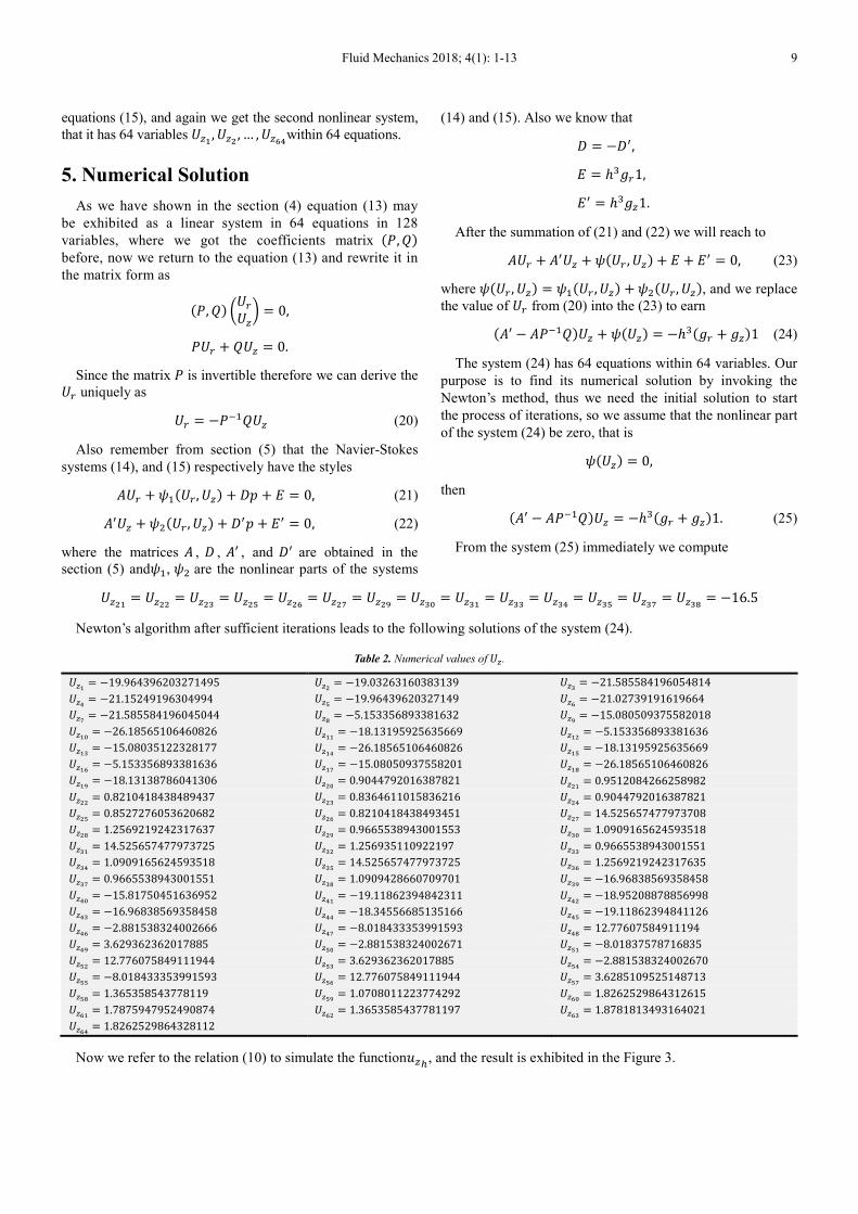
From the system (25) immediately we compute

E L = E = E = E = E = E = E = E = E L = E = E = E = E = E = −16.5

Newton’s algorithm after sufficient iterations leads to the following solutions of the system (24).

Table 2. Numerical values of E . E L = −19.964396203271495 E = −19.03263160383139 E = −21.585584196054814 E = −21.15249196304994 E = −19.96439620327149 E = −21.02739191619664 E = −21.585584196045044 E = −5.153356893381632 E = −15.080509375582018 E L = −26.18565106460826 E LL = −18.13195925635669 E L = −5.153356893381636 E L = −15.08035122328177 E L = −26.18565106460826 E L = −18.13195925635669 E L = −5.153356893381636 E L = −15.08050937558201 E L = −26.18565106460826 E L = −18.13138786041306 E = 0.9044792016387821 E L = 0.9512084266258982 E = 0.8210418438489437 E = 0.8364611015836216 E = 0.9044792016387821 E = 0.8527276053620682 E = 0.8210418438493451 E = 14.525657477973708 E = 1.2569219242317637 E = 0.9665538943001553 E = 1.0909165624593518 E L = 14.525657477973725 E = 1.256935110922197 E = 0.9665538943001551 E = 1.0909165624593518 E = 14.525657477973725 E = 1.2569219242317635 E = 0.9665538943001551 E = 1.0909428660709701 E = −16.96838569358458 E = −15.81750451636952 E L = −19.11862394842311 E = −18.95208878856998 E = −16.96838569358458 E = −18.34556685135166 E = −19.11862394841126 E = −2.881538324002666 E = −8.018433353991593 E = 12.77607584911194 E = 3.629362362017885 E = −2.881538324002671 E L = −8.01837578716835 E = 12.776075849111944 E = 3.629362362017885 E = −2.881538324002670 E = −8.018433353991593 E = 12.776075849111944 E = 3.6285109525148713 E = 1.365358543778119 E = 1.0708011223774292 E = 1.8262529864312615 E L = 1.7875947952490874 E = 1.3653585437781197 E = 1.8781813493164021 E = 1.8262529864328112

Now we refer to the relation (10) to simulate the function (, and the result is exhibited in the Figure 3.



Figure 3. Simulation of the function (.

We insert E valuesto compute the E from (20).

Table 3. Numerical values of E. EL 0.00438008 E = −0.00306589 E = −0.00245443 E = −0.00408989 E = −0.00438008 E = −0.00274863 E = −0.00245443 E = −0.0708664 E = −0.00605582 EL = −0.0030872 ELL = −0.0032878 EL = −0.0708664 EL = −0.0060558 EL = −0.0030872 EL = −0.0032878 EL = −0.0708664 EL = −0.0060558 EL = −0.0030872 EL = −0.0032879 E = −0.0145846 E! = −0.0156674 E = −0.0079492 E = −0.0065575 E = −0.0145846 E = −0.0130577 E = −0.0079492 E = −0.0065490 E = −0.0343992 E = −0.1900569 E = −0.0701881 EL = −0.0065490 E = −0.0343987 E = −0.190056 E = −0.0701881 E = −0.0065490 E = −0.0343992 E = −0.1900564 E = −0.0701836 E = −0.0013567 E = −0.0005378 EL = −0.0046600 E = −0.0030321 E = −0.0013567 E = −0.0049867 E = −0.0046600 E = 0.04687816 E = 0.00385469 E = 0.00610555 E = 0.00566393 E = 0.04687813 EL = 0.00385473 E = 0.00610555 E = 0.00566393 E = 0.0468781 E = 0.00385469 E = 0.00610555 E = 0.00624877 E = −0.0547324 E = −0.0472148 E = −0.0932275 EL = −0.0924344 E = −0.0547324 E = −0.054748 E = −0.0932275

Now we insert the values of E into the relation (9) to simulate the function(, and we will show the result in the Figure 4.


Figure 4. Simulation of the function (.

In the section 5 we have computed the values of E and E , then in the final stage we are ready to determine the coefficients

of energy conservation equation. We can apply the computed values of E and E to earn the linear system of equations in 64

equations in 64 variables. After determining the relevant integrals in 24 tetrahedrons and summation we prepare the necessary

coefficients as

,=== 10ℎ, ,=,=oS;n;oU,= = 0, ,=,=oS;n;oU,=oS;n;oU = 0, ,=,=,=oS;n;oU = 253 ℎ, ,=,=nS;n;oU,= = 0, ,=,=nS;n;oU,=nS;n;oU = 0, ,=,=,=nS;n;oU = 253 ℎ, ¡ = − f ℎ9,

Also we compute the _=X by applying the Mathematica codes, and at last we derive # as

Table 4. Numerical values of #.

# = 267464.5078493500 #! = 248522.6313318577 #9 = 307632.2765236602 #v = 307560.1642197024 #¢ = 279837.7344858227 # = 321624.6206048220 #£ = 427070.98850310955 # = 196160.3580918937 # = 3066.7775345885548 #- = 186800.7827549864 # = 121034.4905810277 #! = 196594.3191942781 #9 = 2152.441237715346 #v = 188106.5416768024 #¢ = 121684.1356482915 # = 197507.5771545514 #£ = −74.8655135629144 # = 191421.1027365251 # = 123429.0998086314 #!- = −13968.2246030608 #! = −12457.9582485794



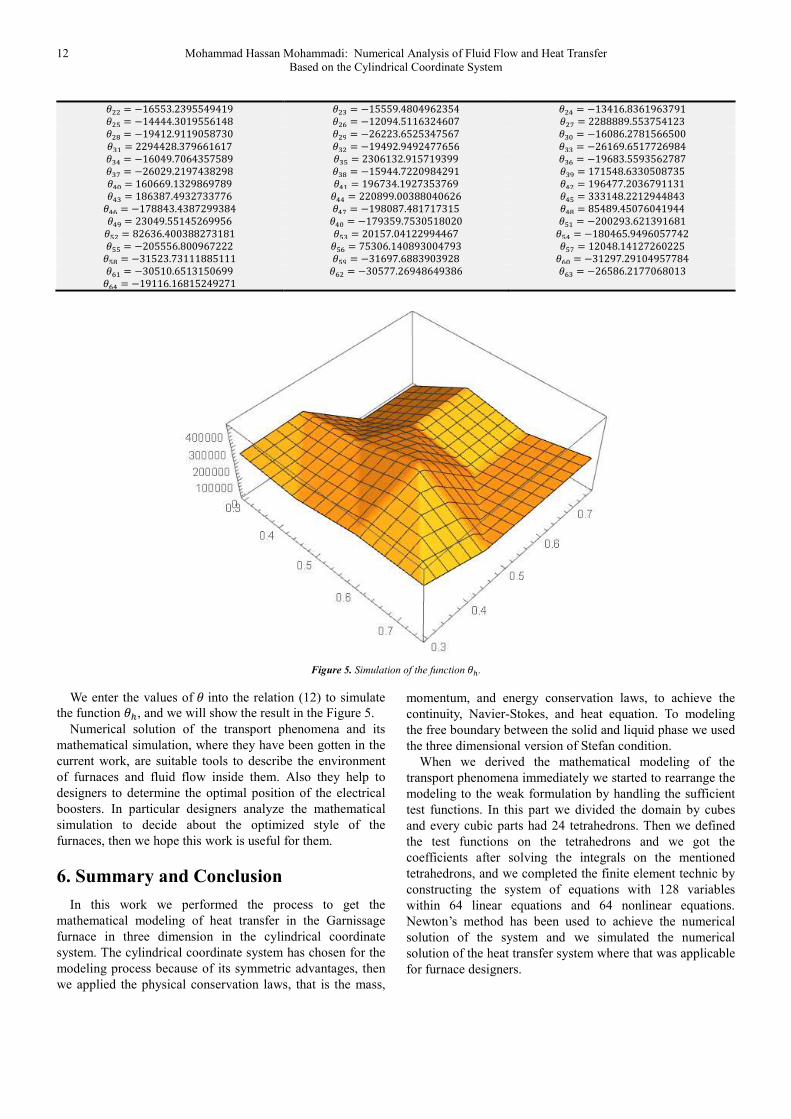
#!! 16553.2395549419 #!9 = −15559.4804962354 #!v = −13416.8361963791 #!¢ = −14444.3019556148 #! = −12094.5116324607 #!£ = 2288889.553754123 #! = −19412.9119058730 #! = −26223.6525347567 #9- = −16086.2781566500 #9 = 2294428.379661617 #9! = −19492.9492477656 #99 = −26169.6517726984 #9v = −16049.7064357589 #9¢ = 2306132.915719399 #9 = −19683.5593562787 #9£ = −26029.2197438298 #9 = −15944.7220984291 #9 = 171548.6330508735 #v- = 160669.1329869789 #v = 196734.1927353769 #v! = 196477.2036791131 #v9 = 186387.4932733776 #vv = 220899.00388040626 #v¢ = 333148.2212944843 #v = −178843.4387299384 #v£ = −198087.481717315 #v = 85489.45076041944 #v = 23049.55145269956 #v- = −179359.7530518020 #¢ = −200293.621391681 #¢! = 82636.400388273181 #¢9 = 20157.04122994467 #¢v = −180465.9496057742 #¢¢ = −205556.800967222 #¢ = 75306.140893004793 #¢£ = 12048.14127260225 #¢ = −31523.73111885111 #¢ = −31697.6883903928 #- = −31297.29104957784 # = −30510.6513150699 #! = −30577.26948649386 #9 = −26586.2177068013 #v = −19116.16815249271

Figure 5. Simulation of the function #(.

We enter the values of # into the relation (12) to simulate

the function #(, and we will show the result in the Figure 5.

Numerical solution of the transport phenomena and its

mathematical simulation, where they have been gotten in the

current work, are suitable tools to describe the environment

of furnaces and fluid flow inside them. Also they help to

designers to determine the optimal position of the electrical

boosters. In particular designers analyze the mathematical

simulation to decide about the optimized style of the

furnaces, then we hope this work is useful for them.

6. Summary and Conclusion

In this work we performed the process to get the

mathematical modeling of heat transfer in the Garnissage

furnace in three dimension in the cylindrical coordinate

system. The cylindrical coordinate system has chosen for the

modeling process because of its symmetric advantages, then

we applied the physical conservation laws, that is the mass,

momentum, and energy conservation laws, to achieve the

continuity, Navier-Stokes, and heat equation. To modeling

the free boundary between the solid and liquid phase we used

the three dimensional version of Stefan condition.

When we derived the mathematical modeling of the

transport phenomena immediately we started to rearrange the

modeling to the weak formulation by handling the sufficient

test functions. In this part we divided the domain by cubes

and every cubic parts had 24 tetrahedrons. Then we defined

the test functions on the tetrahedrons and we got the

coefficients after solving the integrals on the mentioned

tetrahedrons, and we completed the finite element technic by

constructing the system of equations with 128 variables

within 64 linear equations and 64 nonlinear equations.

Newton’s method has been used to achieve the numerical

solution of the system and we simulated the numerical

solution of the heat transfer system where that was applicable

for furnace designers.


Nomenclature

, >, ? cylindrical coordinates ¤ , ¤ approximate velocity components in cylindrical

coordinate , velocity components in cylindrical coordinate "( approximate pressure @ time # temperature , gravity acceleration components h latent heat f specific heat capacity dynamic viscosity ` thermal conductivity density " pressure #( approximate temperature heat source ,- Sobolev space with compact support

References

[1] Ungan A., R. Viskanta, Three-dimensional Numerical Modeling of Circulation and Heat Transfer in a Glass Melting Tank. IEEE Transactions on Industry Applications, Vol. IA-22, No. 5, pp. 922–933, 1986.

[2] Ungan A, R. Viskanta, Three-dimensional Numerical Simulation of Circulation and Heat Transfer in an Electrically Boosted Glass Melting Tank. Part. 2 Sample Simulations, Glastechnische Berichte, Vol. 60, No. 4, pp. 115–124, 1987.

[3] Sadov S. YU., P. N. Shivakumar, D. Firsov, S. H. Lui, R. Thulasiram, Mathematical Model of Ice Melting on Transmission Lines, Journal of Mathematical Modeling and Algorithms, Vol. 6, No. 2, pp. 273-286, 2007.

[4] Pilon L., G. Zhao, and R. Viskanta, Three-Dimensional Flow and Thermal Structures in Glass Melting Furnaces. Part I. effects of the heat flux distribution, Glass Science and Technology, Vol. 75, No. 2, pp. 55–68, 2002.

[5] Pilon L., G. Zhao, and R. Viskanta, Three-Dimensional Flow and Thermal Structures in Glass Melting Furnaces. Part II. Effect of Batch and Bubbles. Glass Science and Technology, Vol. 75, No. 3 pp. 115-124, 2006.

[6] Choudhary Manoj K., Raj Venuturumilli, Matthew R. Hyre, Mathematical Modeling of Flow and Heat Transfer Phenomena in Glass Melting, Delivery, and Forming Processes. International Journal of Applied Glass Science, Vol. 1, No. 2, pp. 188–214, 2010.

[7] Alexiades V., A. D. Solomon, Mathematical Modeling of Melting and Freezing Processes, Hemisphere Publishing Corporation, 1993.

[8] Henry Hu, Stavros A. Argyropoulos, Mathematical Modelling of Solidification and Melting: a Review, Modelling and Simulation in Materials Science and Engineering, Vol. 4, pp. 371-396, 1996.

[9] Rodrigues J. F., Variational Methods in the Stefan Problem,

Lecture Notes in Mathematics, Springer-Verlag, pp. 147-212, 1994.

[10] Vuik C., A. Segal, F. J. Vermolen, a Conserving Discretization for a Stefan Problem with an Interface Reaction at the Free Boundary, Computing and Visualization in Science, Springer-Verlag, Vol. 3, pp. 109-114, 2000.

[11] Byron Bird R., Warren E. Stewart, Edwin N. Lightfoot, Transport Phenomena, John Wiley & Sons, Inc. 2nd Edition, 2002.

[12] Irving H. Shames, Mechanics of Fluids, McGraw-Hill, 4th Edition, 2003.

[13] Robert W. Fox, Alan T. McDonald, Philip J. Pritchard, Introduction to Fluid Mechanics, John Wiley & Sons, Inc. 6th Edition, 2004.

[14] Xu Quan-Sheng, Zhu You-Lan, Solution of the Two-Dimensional Stefan Problem by the Singularity-Separating Method, Journal of Computational Mathematics, Vol. 3, No. 1, pp. 8-18, 1985.

[15] Brenner S., R. Scott, the Mathematical Theory of Finite Element Methods. Springer Verlag, 1994. Corr. 2nd printing 1996.

[16] Johnson C., Numerical Solution of Partial Differential Equations by the Finite Element Method. CUP, 1990.

[17] Epperson J. F., an Introduction to Numerical Methods and Analysis, John Wiley & Sons, Inc. 2002.

[18] Mohammadi M. H., Mathematical Modeling of Heat Transfer and Transport Phenomena in Three-Dimension with Stefan Free Boundary, Advances and Applications in Fluid Mechanics, Vol. 19, No. 1, pp. 23-34, 2016.

[19] Mohammadi M. H., Three-Dimensional Mathematical Modeling of Heat Transfer by Stream Function and its Numerical Solution, Far East Journal of Mathematical Sciences (FJMS), Vol. 99, No. 7, pp. 969-981, 2016.

[20] Babayan A. H., M. H. Mohammadi, the Mathematical Modeling of Garnissage Furnace, NPUA, Bulletin, Collection of Scientific Papers, Part 1, pp. 7-11, 2016.

numerical analysis of fluid flow and heat transfer...

Documents