numerical analysis using matlab and excel
DESCRIPTION
Numerical Analysis Using MATLAB and ExcelTRANSCRIPT
Orchard Publicationswww.orchardpublications.com
NumericalAnalysis
Using MATLAB® and Excel®
Steven T. Karris
Third Edition
ISBN-13: 978-11-9934404-004-11
Orchard PublicationsVisit us on the Internet
www.orchardpublications.comor email us: [email protected]
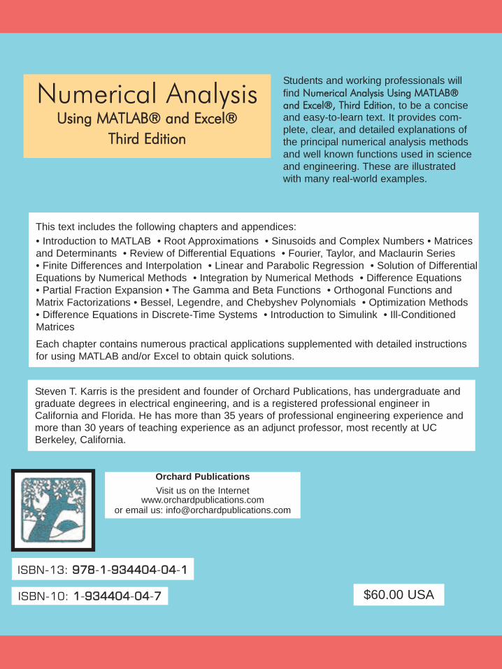
Steven T. Karris is the president and founder of Orchard Publications, has undergraduate andgraduate degrees in electrical engineering, and is a registered professional engineer in California and Florida. He has more than 35 years of professional engineering experience and more than 30 years of teaching experience as an adjunct professor, most recently at UC Berkeley, California.
This text includes the following chapters and appendices:• Introduction to MATLAB • Root Approximations • Sinusoids and Complex Numbers • Matricesand Determinants • Review of Differential Equations • Fourier, Taylor, and Maclaurin Series • Finite Differences and Interpolation • Linear and Parabolic Regression • Solution of DifferentialEquations by Numerical Methods • Integration by Numerical Methods • Difference Equations• Partial Fraction Expansion • The Gamma and Beta Functions • Orthogonal Functions and Matrix Factorizations • Bessel, Legendre, and Chebyshev Polynomials • Optimization Methods• Difference Equations in Discrete-Time Systems • Introduction to Simulink • Ill-ConditionedMatrices
Each chapter contains numerous practical applications supplemented with detailed instructionsfor using MATLAB and/or Excel to obtain quick solutions.
Students and working professionals willfind NNuummeerriiccaall AAnnaallyyssiiss UUssiinngg MMAATTLLAABB®®aanndd EExxcceell®®,, TThhiirrdd EEddiittiioonn, to be a conciseand easy-to-learn text. It provides com-plete, clear, and detailed explanations ofthe principal numerical analysis methodsand well known functions used in scienceand engineering. These are illustratedwith many real-world examples.
Numerical AnalysisUsing MATLAB® and Excel®
Third Edition
$60.00 USAISBN-10: 1-9934404-004-77
Numerical AnalysisUsing MATLAB® and Excel®
Third Edition
Steven T. Karris
Orchard Publicationswww.orchardpublications.com
Numerical Analysis Using MATLAB® and Excel®, Third Edition
Copyright ” 2007 Orchard Publications. All rights reserved. Printed in the United States of America. No part of thispublication may be reproduced or distributed in any form or by any means, or stored in a data base or retrieval system,without the prior written permission of the publisher.
Direct all inquiries to Orchard Publications, [email protected]
Product and corporate names are trademarks or registered trademarks of the Microsoft™ Corporation and TheMathWorks™, Inc. They are used only for identification and explanation, without intent to infringe.
Library of Congress Cataloging-in-Publication Data
Library of Congress Control Number: 2007922100
Copyright TX 5-589-152
ISBN-13: 978-1-934404-04-1
ISBN-10: 1-934404-04-7
Disclaimer
The author has made every effort to make this text as complete and accurate as possible, but no warranty is implied.The author and publisher shall have neither liability nor responsibility to any person or entity with respect to any lossor damages arising from the information contained in this text.
Preface
Numerical analysis is the branch of mathematics that is used to find approximations to difficultproblems such as finding the roots of non−linear equations, integration involving complexexpressions and solving differential equations for which analytical solutions do not exist. It isapplied to a wide variety of disciplines such as business, all fields of engineering, computer science,education, geology, meteorology, and others.
Years ago, high−speed computers did not exist, and if they did, the largest corporations could onlyafford them; consequently, the manual computation required lots of time and hard work. But nowthat computers have become indispensable for research work in science, engineering and otherfields, numerical analysis has become a much easier and more pleasant task.
This book is written primarily for students/readers who have a good background of high−schoolalgebra, geometry, trigonometry, and the fundamentals of differential and integral calculus.* Aprior knowledge of differential equations is desirable but not necessary; this topic is reviewed inChapter 5.
One can use Fortran, Pascal, C, or Visual Basic or even a spreadsheet to solve a difficult problem.It is the opinion of this author that the best applications programs for solving engineeringproblems are 1) MATLAB which is capable of performing advanced mathematical andengineering computations, and 2) the Microsoft Excel spreadsheet since the versatility offered byspreadsheets have revolutionized the personal computer industry. We will assume that the readerhas no prior knowledge of MATLAB and limited familiarity with Excel.
We intend to teach the student/reader how to use MATLAB via practical examples and fordetailed explanations he/she will be referred to an Excel reference book or the MATLAB User’sGuide. The MATLAB commands, functions, and statements used in this text can be executedwith either MATLAB Student Version 12 or later. Our discussions are based on a PC withWindows XP platforms but if you have another platform such as Macintosh, please refer to theappropriate sections of the MATLAB’s User Guide that also contains instructions for installation.
MATLAB is an acronym for MATrix LABoratory and it is a very large computer applicationwhich is divided to several special application fields referred to as toolboxes. In this book we willbe using the toolboxes furnished with the Student Edition of MATLAB. As of this writing, thelatest release is MATLAB Student Version Release 14 and includes SIMULINK which is a
* These topics are discussed in Mathematics for Business, Science, and Technology, Third Edition, ISBN 0−9709511−0−8. This text includes probability and other advanced topics which are supplemented by many practical applications usingMicrosoft Excel and MATLAB.
software package used for modeling, simulating, and analyzing dynamic systems. SIMULINK isnot discussed in this text; the interested reader may refer to Introduction to Simulink withEngineering Applications, ISBN 0−9744239−7−1. Additional information including purchasingthe software may be obtained from The MathWorks, Inc., 3 Apple Hill Drive, Natick, MA01760−2098. Phone: 508 647−7000, Fax: 508 647−7001, e−mail: [email protected] and website http://www.mathworks.com.
The author makes no claim to originality of content or of treatment, but has taken care to presentdefinitions, statements of physical laws, theorems, and problems.
Chapter 1 is an introduction to MATLAB. The discussion is based on MATLAB Student Version5 and it is also applicable to Version 6. Chapter 2 discusses root approximations by numericalmethods. Chapter 3 is a review of sinusoids and complex numbers. Chapter 4 is an introduction tomatrices and methods of solving simultaneous algebraic equations using Excel and MATLAB.Chapter 5 is an abbreviated, yet practical introduction to differential equations, state variables,state equations, eigenvalues and eigenvectors. Chapter 6 discusses the Taylor and Maclaurinseries. Chapter 7 begins with finite differences and interpolation methods. It concludes withapplications using MATLAB. Chapter 8 is an introduction to linear and parabolic regression.Chapters 9 and 10 discuss numerical methods for differentiation and integration respectively.Chapter 11 is a brief introduction to difference equations with a few practical applications.Chapters 12 is devoted to partial fraction expansion. Chapters 13, 14, and 15 discuss certaininteresting functions that find wide application in science, engineering, and probability. This textconcludes with Chapter 16 which discusses three popular optimization methods.
New to the Third Edition
This is an extensive revision of the first edition. The most notable changes are the inclusion ofFourier series, orthogonal functions and factorization methods, and the solutions to all end−of−chapter exercises. It is in response to many readers who expressed a desire to obtain the solutionsin order to check their solutions to those of the author and thereby enhancing their knowledge.Another reason is that this text is written also for self−study by practicing engineers who need areview before taking more advanced courses such as digital image processing. The author hasprepared more exercises and they are available with their solutions to those instructors who adoptthis text for their class.
Another change is the addition of a rather comprehensive summary at the end of each chapter.Hopefully, this will be a valuable aid to instructors for preparation of view foils for presenting thematerial to their class.
The last major change is the improvement of the plots generated by the latest revisions of theMATLAB® Student Version, Release 14.
Orchard PublicationsFremont, Californiawww.orchardpublications.cominfo@orchardpublications.com
Numerical Analysis Using MATLAB® and Excel®, Third Edition iCopyright © Orchard Publications
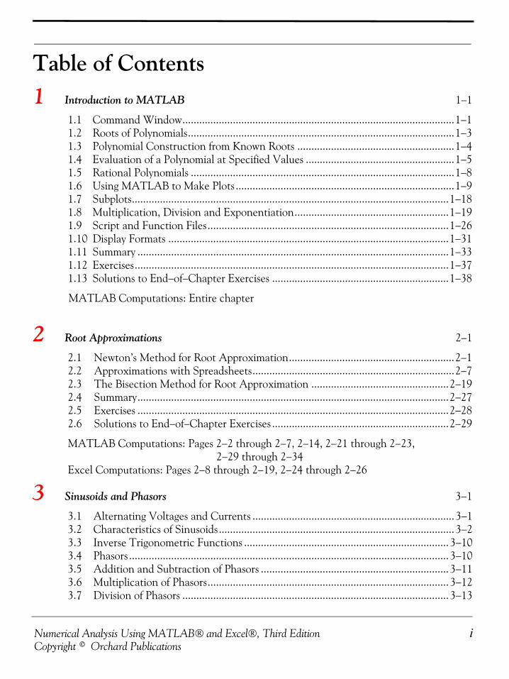
Table of Contents1 Introduction to MATLAB 1−1
1.1 Command Window.................................................................................................1−11.2 Roots of Polynomials...............................................................................................1−31.3 Polynomial Construction from Known Roots ........................................................1−41.4 Evaluation of a Polynomial at Specified Values .....................................................1−51.5 Rational Polynomials ..............................................................................................1−81.6 Using MATLAB to Make Plots ..............................................................................1−91.7 Subplots.................................................................................................................1−181.8 Multiplication, Division and Exponentiation.......................................................1−191.9 Script and Function Files......................................................................................1−261.10 Display Formats ....................................................................................................1−311.11 Summary ...............................................................................................................1−331.12 Exercises................................................................................................................1−371.13 Solutions to End−of−Chapter Exercises ...............................................................1−38
MATLAB Computations: Entire chapter
2 Root Approximations 2−1
2.1 Newton’s Method for Root Approximation...........................................................2−12.2 Approximations with Spreadsheets........................................................................2−72.3 The Bisection Method for Root Approximation .................................................2−192.4 Summary...............................................................................................................2−272.5 Exercises ...............................................................................................................2−282.6 Solutions to End−of−Chapter Exercises ...............................................................2−29
MATLAB Computations: Pages 2−2 through 2−7, 2−14, 2−21 through 2−23, 2−29 through 2−34
Excel Computations: Pages 2−8 through 2−19, 2−24 through 2−26
3 Sinusoids and Phasors 3−1
3.1 Alternating Voltages and Currents ........................................................................ 3−13.2 Characteristics of Sinusoids.................................................................................... 3−23.3 Inverse Trigonometric Functions ......................................................................... 3−103.4 Phasors .................................................................................................................. 3−103.5 Addition and Subtraction of Phasors ................................................................... 3−113.6 Multiplication of Phasors...................................................................................... 3−123.7 Division of Phasors ............................................................................................... 3−13
ii Numerical Analysis Using MATLAB® and Excel®, Third EditionCopyright © Orchard Publications
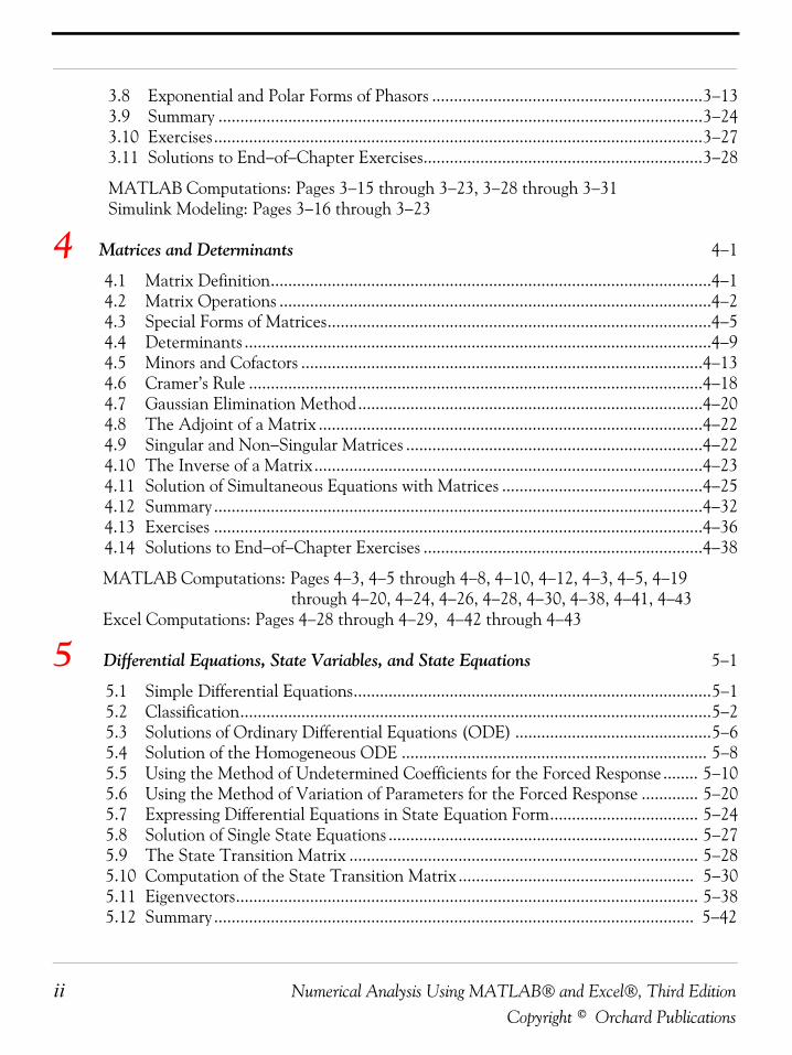
3.8 Exponential and Polar Forms of Phasors ..............................................................3−133.9 Summary ...............................................................................................................3−243.10 Exercises................................................................................................................3−273.11 Solutions to End−of−Chapter Exercises................................................................3−28
MATLAB Computations: Pages 3−15 through 3−23, 3−28 through 3−31 Simulink Modeling: Pages 3−16 through 3−23
4 Matrices and Determinants 4−1
4.1 Matrix Definition.....................................................................................................4−14.2 Matrix Operations ...................................................................................................4−24.3 Special Forms of Matrices........................................................................................4−54.4 Determinants ...........................................................................................................4−94.5 Minors and Cofactors ............................................................................................4−134.6 Cramer’s Rule ........................................................................................................4−184.7 Gaussian Elimination Method...............................................................................4−204.8 The Adjoint of a Matrix ........................................................................................4−224.9 Singular and Non−Singular Matrices ....................................................................4−224.10 The Inverse of a Matrix.........................................................................................4−234.11 Solution of Simultaneous Equations with Matrices ..............................................4−254.12 Summary ................................................................................................................4−324.13 Exercises ................................................................................................................4−364.14 Solutions to End−of−Chapter Exercises ................................................................4−38
MATLAB Computations: Pages 4−3, 4−5 through 4−8, 4−10, 4−12, 4−3, 4−5, 4−19 through 4−20, 4−24, 4−26, 4−28, 4−30, 4−38, 4−41, 4−43
Excel Computations: Pages 4−28 through 4−29, 4−42 through 4−43
5 Differential Equations, State Variables, and State Equations 5−1
5.1 Simple Differential Equations..................................................................................5−15.2 Classification............................................................................................................5−25.3 Solutions of Ordinary Differential Equations (ODE) .............................................5−65.4 Solution of the Homogeneous ODE ...................................................................... 5−85.5 Using the Method of Undetermined Coefficients for the Forced Response ........ 5−105.6 Using the Method of Variation of Parameters for the Forced Response ............. 5−205.7 Expressing Differential Equations in State Equation Form.................................. 5−245.8 Solution of Single State Equations ....................................................................... 5−275.9 The State Transition Matrix ................................................................................ 5−285.10 Computation of the State Transition Matrix ...................................................... 5−305.11 Eigenvectors.......................................................................................................... 5−385.12 Summary .............................................................................................................. 5−42
Numerical Analysis Using MATLAB® and Excel®, Third Edition iiiCopyright © Orchard Publications
5.13 Exercises ............................................................................................................... 5−475.14 Solutions to End−of−Chapter Exercises............................................................... 5−49
MATLAB Computations: Pages 5−11, 5−13 through 5−14, 5−16 through 5−17,5−19, 5−23, 5−33 through 5−35, 5−37,5−49 through 5−53, 5−55
6 Fourier, Taylor, and Maclaurin Series 6−1
6.1 Wave Analysis ........................................................................................................6−16.2 Evaluation of the Coefficients ...............................................................................6−26.3 Symmetry ...............................................................................................................6−76.4 Waveforms in Trigonometric Form of Fourier Series .........................................6−126.5 Alternate Forms of the Trigonometric Fourier Series .........................................6−256.6 The Exponential Form of the Fourier Series .......................................................6−296.7 Line Spectra .........................................................................................................6−336.8 Numerical Evaluation of Fourier Coefficients .....................................................6−366.9 Power Series Expansion of Functions ..................................................................6−406.10 Taylor and Maclaurin Series ................................................................................6−416.11 Summary ..............................................................................................................6−486.12 Exercises ..............................................................................................................6−516.13 Solutions to End−of−Chapter Exercises ..............................................................6−53
MATLAB Computations: Pages 6−35, 6−45, 6−58 through 6−61Excel Computations: Pages 6−37 through 6−39
7 Finite Differences and Interpolation 7−1
7.1 Divided Differences ............................................................................................... 7−17.2 Factorial Polynomials ............................................................................................. 7−67.3 Antidifferences ................................................................................................... 7−127.4 Newton’s Divided Difference Interpolation Method ......................................... 7−157.5 Lagrange’s Interpolation Method ........................................................................ 7−177.6 Gregory−Newton Forward Interpolation Method .............................................. 7−197.7 Gregory−Newton Backward Interpolation Method ........................................... 7−217.8 Interpolation with MATLAB ............................................................................. 7−247.9 Summary ............................................................................................................. 7−397.10 Exercises ............................................................................................................. 7−447.11 Solutions to End−of−Chapter Exercises ............................................................. 7−45
MATLAB Computations: Pages 7−8 through 7−9, 7−13 through 7−15,7−26 through 7−38, 7−45 through 7−46,7−48, 7−50, 7−52
Excel Computations: Pages 7−17 through 7−19, 7−22 through 7−25, 7−49, 7−52
iv Numerical Analysis Using MATLAB® and Excel®, Third EditionCopyright © Orchard Publications
8 Linear and Parabolic Regression 8−1
8.1 Curve Fitting ..........................................................................................................8−18.2 Linear Regression ...................................................................................................8−28.3 Parabolic Regression ..............................................................................................8−78.4 Regression with Power Series Approximations ....................................................8−148.5 Summary ..............................................................................................................8−248.6 Exercises ...............................................................................................................8−268.7 Solutions to End−of−Chapter Exercises ...............................................................8−28
MATLAB Computations: Pages 8−11 through 8−14, 8−17 through 8−23,8−30 through 8−34
Excel Computations: Pages 8−5 through 8−10, 8−15 through 8−19, 8−28 through 8−32
9 Solution of Differential Equations by Numerical Methods 9−1
9.1 Taylor Series Method ............................................................................................ 9−19.2 Runge−Kutta Method ............................................................................................ 9−59.3 Adams’ Method ................................................................................................... 9−139.4 Milne’s Method .................................................................................................... 9−159.5 Summary .............................................................................................................. 9−179.6 Exercises .............................................................................................................. 9−209.7 Solutions to End−of−Chapter Exercises .............................................................. 9−21
MATLAB Computations: Pages 9−5, 9−9 through 9−12, 9−21 through 9−23Excel Computations: Page 9−2, 9−14, 9−22 through 9−26
10 Integration by Numerical Methods 10−1
10.1 The Trapezoidal Rule .......................................................................................... 10−110.2 Simpson’s Rule ..................................................................................................... 10−610.3 Summary ............................................................................................................ 10−1410.4 Exercises ............................................................................................................ 10−1510.5 Solution to End−of−Chapter Exercises .............................................................. 10−16
MATLAB Computations: Pages 10−3 through 10−6, 10−9 through 10−13,10−16, 10−18 through 10−21
Excel Computations: Pages 10−10, 10−19 through 10−21
11 Difference Equations 11−1
11.1 Introduction ......................................................................................................... 11−111.2 Definition, Solutions, and Applications .............................................................. 11−111.3 Fibonacci Numbers .............................................................................................. 11−7
Numerical Analysis Using MATLAB® and Excel®, Third Edition vCopyright © Orchard Publications
11.4 Summary .............................................................................................................11−1111.5 Exercises ............................................................................................................. 11−1311.6 Solutions to End−of−Chapter Exercises .............................................................11−14
12 Partial Fraction Expansion 12−1
12.1 Partial Fraction Expansion ..................................................................................12−112.2 Alternate Method of Partial Fraction Expansion ..............................................12−1312.3 Summary ............................................................................................................12−1912.4 Exercises ............................................................................................................12−2212.5 Solutions to End−of−Chapter Exercises ............................................................12−23
MATLAB Computations: Pages 12−3 through 12−5, 12−9 through 12−12,12−16 through 12-18, 12−23 through 12−28
13 The Gamma and Beta Functions and Distributions 13−1
13.1 The Gamma Function .........................................................................................13−113.2 The Gamma Distribution ..................................................................................13−1613.3 The Beta Function .............................................................................................13−1713.4 The Beta Distribution ........................................................................................13−2013.5 Summary ............................................................................................................13−2213.6 Exercises ............................................................................................................13−2413.7 Solutions to End−of−Chapter Exercises ............................................................13−25
MATLAB Computations: Pages 13−3, 13−5, 13−10, 13−19, 13−25Excel Computations: Pages 13−5, 13−10, 13−16 through 13−17, 13−19, 13−21
14 Orthogonal Functions and Matrix Factorizations 14−1
14.1 Orthogonal Functions ......................................................................................14−114.2 Orthogonal Trajectories ...................................................................................14−214.3 Orthogonal Vectors ..........................................................................................14−414.4 The Gram−Schmidt Orthogonalization Procedure ..........................................14−714.5 The LU Factorization .......................................................................................14−914.6 The Cholesky Factorization ............................................................................14−2314.7 The QR Factorization .....................................................................................14−2514.8 Singular Value Decomposition .......................................................................14−2814.9 Summary .........................................................................................................14−3014.10 Exercises .........................................................................................................14−3214.11 Solutions to End−of−Chapter Exercises .........................................................14−34
MATLAB Computations: Pages 14−8 through 14−9, 14−11 through 14−29,14−36, 14−38 through 14−39
vi Numerical Analysis Using MATLAB® and Excel®, Third EditionCopyright © Orchard Publications
15 Bessel, Legendre, and Chebyshev Functions 15−1
15.1 The Bessel Function ............................................................................................15−115.2 Legendre Functions ...........................................................................................15−1015.3 Laguerre Polynomials .........................................................................................15−2115.4 Chebyshev Polynomials .....................................................................................15−2215.5 Summary ............................................................................................................15−2715.6 Exercises .............................................................................................................15−3215.7 Solutions to End−of−Chapter Exercises ............................................................15−33
MATLAB Computations: Pages 15−3 through 15−4, 15−6, 15−9, 14−19 through 15−22, 15−25, 15−33, 15−35 through 15−37
Excel Computations: Pages 15−5, 15−9
16 Optimization Methods 16−1
16.1 Linear Programming ........................................................................................... 16−116.2 Dynamic Programming ........................................................................................16−416.3 Network Analysis ...............................................................................................16−1416.4 Summary ............................................................................................................16−1916.5 Exercises .............................................................................................................15−2016.6 Solutions to End−of−Chapter Exercises ............................................................15−22
MATLAB Computations: Pages 16−3Excel Computations: Pages 16−4, 16−23, 16−25 through 16−27
A Difference Equations in Discrete−Time Systems A−1
A.1 Recursive Method for Solving Difference Equations........................................... A−1A.2 Method of Undetermined Coefficients ................................................................A−1
MATLAB Computations: Pages A−4, A−7, A−9
B Introduction to Simulink® B−1
B.1 Simulink and its Relation to MATLAB ...............................................................B−1B.2 Simulink Demos ..................................................................................................B−20
MATLAB Computations and Simulink Modeling: Entire Appendix B
C Ill-Conditioned Matrices C−1
C.1 The Norm of a Matrix ...........................................................................................C−1C.2 Condition Number of a Matrix .............................................................................C−2C.3 Hilbert Matrices ....................................................................................................C−3
Numerical Analysis Using MATLAB® and Excel®, Third Edition viiCopyright © Orchard Publications
MATLAB Computations: Pages C−1, C−4 through C−5
References R−1
Index IN−1
Numerical Analysis Using MATLAB® and Excel®, Third Edition 1−1Copyright © Orchard Publications
Chapter 1
Introduction to MATLAB
his chapter is an introduction of the basic MATLAB commands and functions, proceduresfor naming and saving the user generated files, comment lines, access to MATLAB’s Editor/Debugger, finding the roots of a polynomial, and making plots. Several examples are pro-
vided with detailed explanations. Throughout this text, a left justified horizontal bar will denotethe beginning of an example, and a right justified horizontal bar will denote the end of the exam-ple. These bars will not be shown whenever an example begins at the top of a page or at the bot-tom of a page. Also, when one example follows immediately after a previous example, the rightjustified bar will be omitted.
1.1 Command WindowTo distinguish the screen displays from the user commands, important terms and MATLAB func-tions, we will use the following conventions:
Click: Click the left button of the mouse
Courier Font: Screen displaysHelvetica Font: User inputs at MATLAB’s command window prompt EDU>>*
Helvetica Bold: MATLAB functions
Bold Italic: Important terms and facts, notes, and file names
When we first start MATLAB, we see the toolbar on top of the command screen and the promptEDU>>. This prompt is displayed also after execution of a command; MATLAB now waits for anew command from the user. We can use the Editor/Debugger to write our program, save it, andreturn to the command screen to execute the program as explained below.
To use the Editor/Debugger:
1. From the File menu on the toolbar, we choose New and click on M−File. This takes us to theEditor Window where we can type our script (list of statements) for a new file, or open a previ-ously saved file. We must save our program with a file name which starts with a letter. Impor-tant! MATLAB is case sensitive, that is, it distinguishes between upper− and lower−case let-ters. Thus, t and T are two different characters in MATLAB language. The files that we createare saved with the file name we use and the extension .m; for example, myfile01.m. It is a good
* EDU>> is the MATLAB prompt in the Student Version.
T
Chapter 1 Introduction to MATLAB
1−2 Numerical Analysis Using MATLAB® and Excel®, Third EditionCopyright © Orchard Publications
practice to save the script in a file name that is descriptive of our script content. For instance, ifthe script performs some matrix operations, we ought to name and save that file asmatrices01.m or any other similar name. We should also use a separate disk to backup our files.
2. Once the script is written and saved as an m−file, we may exit the Editor/Debugger window byclicking on Exit Editor/Debugger of the File menu, and MATLAB returns to the commandwindow.
3. To execute a program, we type the file name without the .m extension at the EDU>> prompt;then, we press <enter> and observe the execution and the values obtained from it. If we havesaved our file in drive a or any other drive, we must make sure that it is added it to the desireddirectory in MATLAB’s search path. The MATLAB User’s Guide provides more informationon this topic.
Henceforth, it will be understood that each input command is typed after the EDU>> promptand followed by the <enter> key.
The command help matlab iofun will display input/output information. To get help with otherMATLAB topics, we can type help followed by any topic from the displayed menu. For example, toget information on graphics, we type help matlab graphics. We can also get help from the Help pull−down menu. The MATLAB User’s Guide contains numerous help topics.
To appreciate MATLAB’s capabilities, we type demo and we see the MATLAB Demos menu. Wecan do this periodically to become familiar with them. Whenever we want to return to the com-mand window, we click on the Close button.
When we are done and want to leave MATLAB, we type quit or exit. But if we want to clear allprevious values, variables, and equations without exiting, we should use the clear command. Thiscommand erases everything; it is like exiting MATLAB and starting it again. The clc commandclears the screen but MATLAB still remembers all values, variables and equations which we havealready used. In other words, if we want MATLAB to retain all previously entered commands, butleave only the EDU>> prompt on the upper left of the screen, we can use the clc command.
All text after the % (percent) symbol is interpreted by MATLAB as a comment line and thus it isignored during the execution of a program. A comment can be typed on the same line as the func-tion or command or as a separate line. For instance, the statements
conv(p,q) % performs multiplication of polynomials p and q
% The next statement performs partial fraction expansion of p(x) / q(x)
are both correct.
One of the most powerful features of MATLAB is the ability to do computations involving com-plex numbers. We can use either , or to denote the imaginary part of a complex number, such as
or . For example, the statement
z=3−4j
i j3 4i– 3 4j–
Numerical Analysis Using MATLAB® and Excel®, Third Edition 1−3Copyright © Orchard Publications
Roots of Polynomials
displays
z = 3.0000 - 4.0000i
In the example above, a multiplication (*) sign between and was not necessary because thecomplex number consists of numerical constants. However, if the imaginary part is a function orvariable such as , we must use the multiplication sign, that is, we must type cos(x)*j orj*cos(x).
1.2 Roots of Polynomials
In MATLAB, a polynomial is expressed as a row vector of the form . The
elements of this vector are the coefficients of the polynomial in descending order. We mustinclude terms whose coefficients are zero.
We can find the roots of any polynomial with the roots(p) function where p is a row vector con-taining the polynomial coefficients in descending order.
Example 1.1 Find the roots of the polynomial
(1.1)Solution:
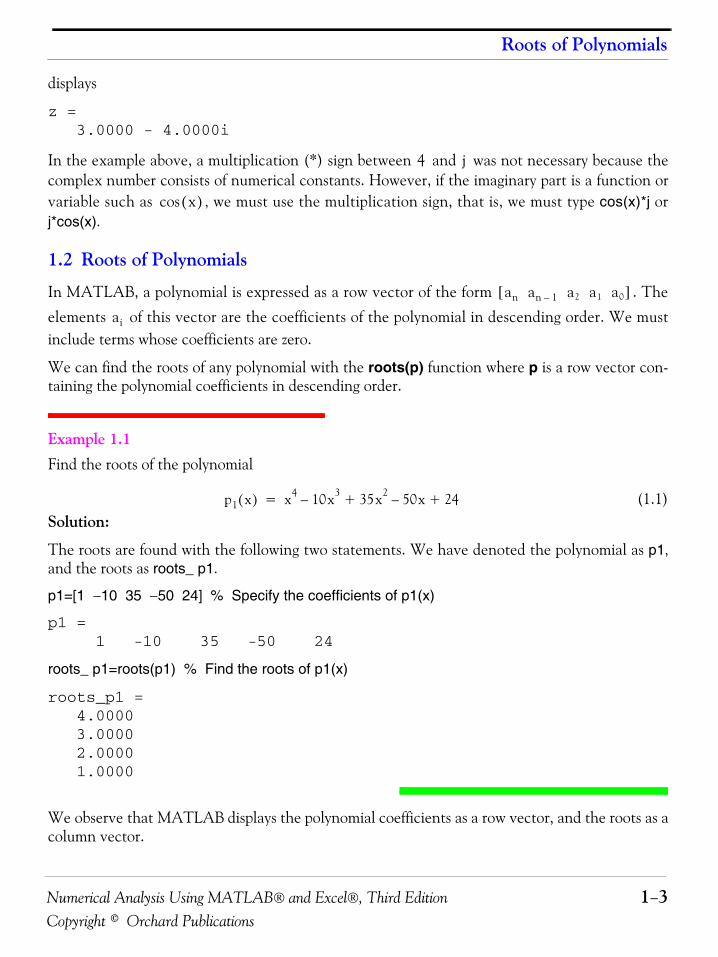
The roots are found with the following two statements. We have denoted the polynomial as p1,and the roots as roots_ p1.
p1=[1 −10 35 −50 24] % Specify the coefficients of p1(x)
p1 = 1 -10 35 -50 24
roots_ p1=roots(p1) % Find the roots of p1(x)
roots_p1 = 4.0000 3.0000 2.0000 1.0000
We observe that MATLAB displays the polynomial coefficients as a row vector, and the roots as acolumn vector.
4 j
x( )cos
an an 1– a2 a1 a0[ ]ai
p1 x( ) x4 10x3– 35x2 50x– 24+ +=
Chapter 1 Introduction to MATLAB
1−4 Numerical Analysis Using MATLAB® and Excel®, Third EditionCopyright © Orchard Publications
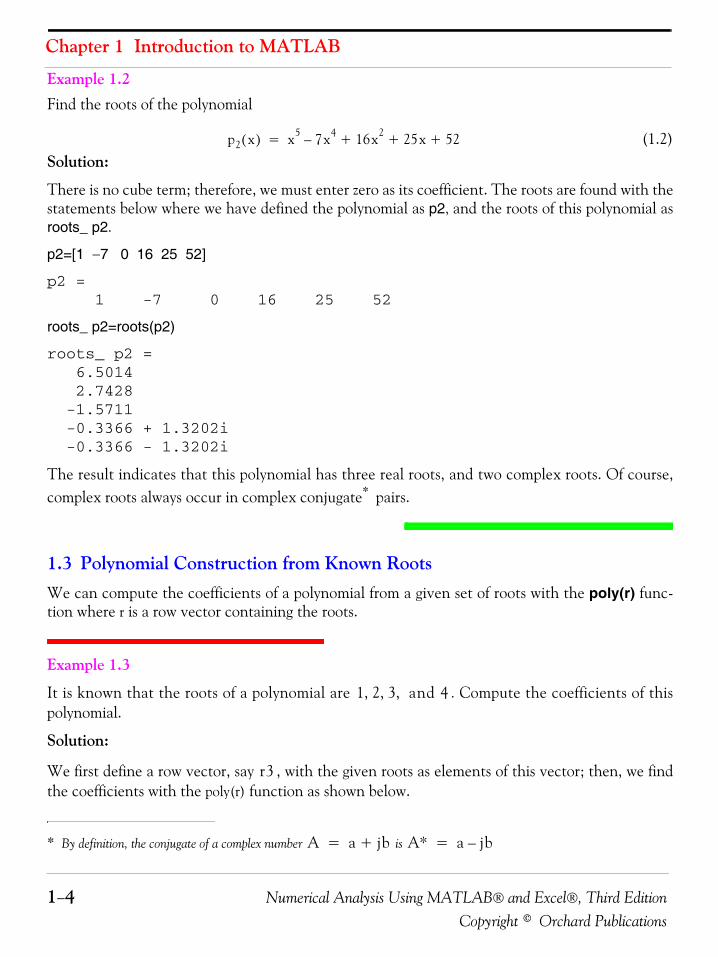
Example 1.2 Find the roots of the polynomial
(1.2)Solution:
There is no cube term; therefore, we must enter zero as its coefficient. The roots are found with thestatements below where we have defined the polynomial as p2, and the roots of this polynomial asroots_ p2.
p2=[1 −7 0 16 25 52]
p2 = 1 -7 0 16 25 52
roots_ p2=roots(p2)
roots_ p2 = 6.5014 2.7428 -1.5711 -0.3366 + 1.3202i -0.3366 - 1.3202i
The result indicates that this polynomial has three real roots, and two complex roots. Of course,complex roots always occur in complex conjugate* pairs.
1.3 Polynomial Construction from Known RootsWe can compute the coefficients of a polynomial from a given set of roots with the poly(r) func-tion where r is a row vector containing the roots.
Example 1.3
It is known that the roots of a polynomial are . Compute the coefficients of thispolynomial.
Solution:
We first define a row vector, say , with the given roots as elements of this vector; then, we findthe coefficients with the poly(r) function as shown below.
* By definition, the conjugate of a complex number is
p2 x( ) x5 7x4– 16x2 25x+ + 52+=
A a jb+= A∗ a jb–=
1 2 3 and 4, , ,
r3
Numerical Analysis Using MATLAB® and Excel®, Third Edition 1−5Copyright © Orchard Publications
Evaluation of a Polynomial at Specified Values
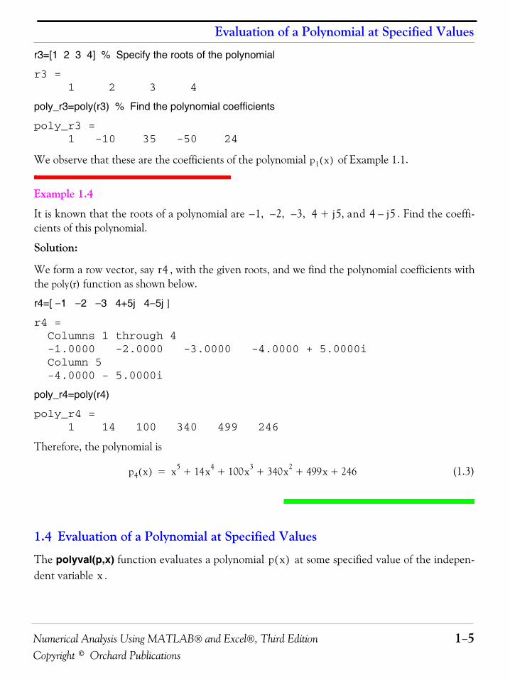
r3=[1 2 3 4] % Specify the roots of the polynomial
r3 = 1 2 3 4
poly_r3=poly(r3) % Find the polynomial coefficients
poly_r3 = 1 -10 35 -50 24
We observe that these are the coefficients of the polynomial of Example 1.1.
Example 1.4
It is known that the roots of a polynomial are . Find the coeffi-cients of this polynomial.
Solution:
We form a row vector, say , with the given roots, and we find the polynomial coefficients withthe poly(r) function as shown below.
r4=[ −1 −2 −3 4+5j 4−5j ]
r4 = Columns 1 through 4 -1.0000 -2.0000 -3.0000 -4.0000 + 5.0000i Column 5 -4.0000 - 5.0000i
poly_r4=poly(r4)
poly_r4 = 1 14 100 340 499 246
Therefore, the polynomial is
(1.3)
1.4 Evaluation of a Polynomial at Specified Values
The polyval(p,x) function evaluates a polynomial at some specified value of the indepen-dent variable .
p1 x( )
1 2 3 4 j5 and 4, j5–+,–,–,–
r4
p4 x( ) x5 14x4 100x3 340x2 499x 246+ + + + +=
p x( )x
Chapter 1 Introduction to MATLAB
1−6 Numerical Analysis Using MATLAB® and Excel®, Third EditionCopyright © Orchard Publications
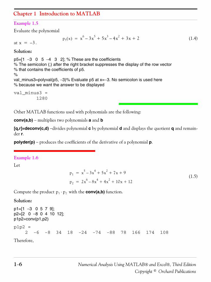
Example 1.5 Evaluate the polynomial
(1.4)at .
Solution:
p5=[1 −3 0 5 −4 3 2]; % These are the coefficients% The semicolon (;) after the right bracket suppresses the display of the row vector% that contains the coefficients of p5.%val_minus3=polyval(p5, −3)% Evaluate p5 at x=−3. No semicolon is used here% because we want the answer to be displayed
val_minus3 = 1280
Other MATLAB functions used with polynomials are the following:
conv(a,b) − multiplies two polynomials a and b
[q,r]=deconv(c,d) −divides polynomial c by polynomial d and displays the quotient q and remain-der r.
polyder(p) − produces the coefficients of the derivative of a polynomial p.
Example 1.6 Let
(1.5)
Compute the product with the conv(a,b) function.
Solution:
p1=[1 −3 0 5 7 9];p2=[2 0 −8 0 4 10 12];p1p2=conv(p1,p2)
p1p2 = 2 -6 -8 34 18 -24 -74 -88 78 166 174 108
Therefore,
p5 x( ) x6 3x5– 5x3 4x2– 3x 2+ + +=x 3–=
p1 x5 3x4– 5x2 7x 9+ + +=
p2 2x6 8x4– 4x2 10x 12+ + +=
p1 p2⋅
Numerical Analysis Using MATLAB® and Excel®, Third Edition 1−7Copyright © Orchard Publications
Evaluation of a Polynomial at Specified Values
We can write MATLAB statements in one line if we separate them by commas or semicolons.Commas will display the results whereas semicolons will suppress the display.
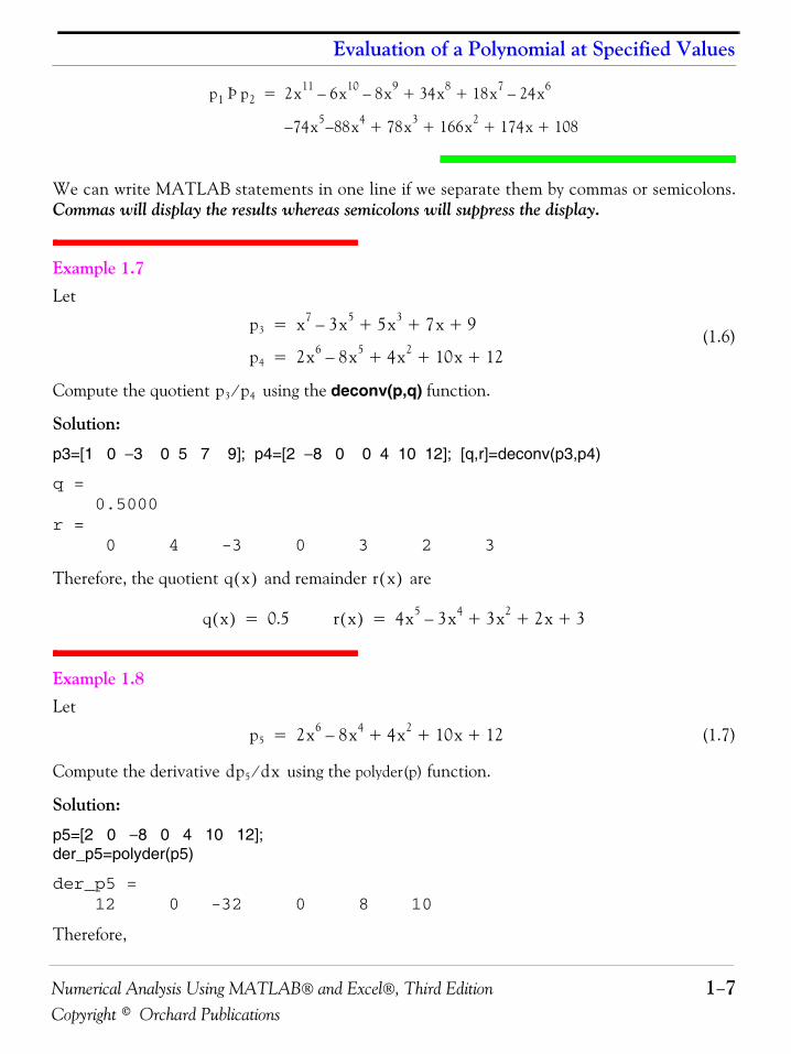
Example 1.7 Let
(1.6)
Compute the quotient using the deconv(p,q) function.
Solution:
p3=[1 0 −3 0 5 7 9]; p4=[2 −8 0 0 4 10 12]; [q,r]=deconv(p3,p4)
q = 0.5000r = 0 4 -3 0 3 2 3
Therefore, the quotient and remainder are
Example 1.8 Let
(1.7)
Compute the derivative using the polyder(p) function.
Solution:
p5=[2 0 −8 0 4 10 12];der_p5=polyder(p5)
der_p5 = 12 0 -32 0 8 10
Therefore,
p1 p2Þ 2x11 6x10 8x9–– 34x8 18x7 24x6–+ +=
74x5 88x4 78x3 166x2 174x 108+ + + +––
p3 x7 3x5– 5x3 7x 9+ + +=
p4 2x6 8x5– 4x2 10x 12+ + +=
p3 p4⁄
q x( ) r x( )
q x( ) 0.5= r x( ) 4x5 3x4– 3x2 2x 3+ + +=
p5 2x6 8x4– 4x2 10x 12+ + +=
dp5 dx⁄
Chapter 1 Introduction to MATLAB
1−8 Numerical Analysis Using MATLAB® and Excel®, Third EditionCopyright © Orchard Publications
1.5 Rational PolynomialsRational Polynomials are those which can be expressed in ratio form, that is, as
(1.8)
where some of the terms in the numerator and/or denominator may be zero. We can find the rootsof the numerator and denominator with the roots(p) function as before.
Example 1.9 Let
(1.9)
Express the numerator and denominator in factored form, using the roots(p) function.
Solution:
num=[1 −3 0 5 7 9]; den=[2 0 −8 0 4 10 12];% Do not display num and den coefficientsroots_num=roots(num), roots_den=roots(den) % Display num and den roots
roots_num = 2.4186 + 1.0712i 2.4186 - 1.0712i -1.1633 -0.3370 + 0.9961i -0.3370 - 0.9961i
roots_den = 1.6760 + 0.4922i 1.6760 - 0.4922i -1.9304 -0.2108 + 0.9870i -0.2108 - 0.9870i -1.0000
As expected, the complex roots occur in complex conjugate pairs.
For the numerator, we have the factored form
and for the denominator, we have
dp5 dx⁄ 12x5 32x3– 4x2 8x 10+ + +=
R x( ) Num x( )Den x( )---------------------
bnxn bn 1– xn 1– bn 2– xn 2– … b1x b0+ + + + +
amxm am 1– xm 1– am 2– xm 2– … a1x a0+ + + + +-------------------------------------------------------------------------------------------------------------------------= =
R x( )pnum
pden------------ x5 3x4– 5x2 7x 9+ + +
2x6 8x4– 4x2 10x 12+ + +-----------------------------------------------------------------------= =
pnum x 2.4186– j1.0712–( ) x 2.4186– j1.0712+( ) x 1.1633+( ) ⋅ ⋅ ⋅=
x 0.3370 j0.9961–+( ) x 0.3370 j0.9961+ +( )⋅
pden x 1.6760– j0.4922–( ) x 1.6760– j0.4922+( ) x 1.9304+( ) ⋅ ⋅ ⋅=
x 0.2108 j– 0.9870+( ) x 0.2108 j0.9870+ +( ) x 1.0000+( )⋅ ⋅
Numerical Analysis Using MATLAB® and Excel®, Third Edition 1−9Copyright © Orchard Publications
Using MATLAB to Make Plots
We can also express the numerator and denominator of this rational function as a combination ofl inear and quadratic factors. We recall that in a quadratic equation of the form
whose roots are and , the negative sum of the roots is equal to the coef-
ficient of the term, that is, , while the product of the roots is equal to the
constant term , that is, . Accordingly, we form the coefficient by addition of thecomplex conjugate roots and this is done by inspection; then we multiply the complex conjugateroots to obtain the constant term using MATLAB as indicated below.
(2.4186+1.0712i)*(2.4186 −1.0712i) % Form the product of the 1st set of complex conjugates
ans = 6.9971
(−0.3370+0.9961i)*(−0.3370−0.9961i) % Form the product of the 2nd set of complex conjugates
ans = 1.1058
(1.6760+0.4922i)*(1.6760−0.4922i)
ans = 3.0512
(−0.2108+0.9870i)*(−0.2108−0.9870i)
ans = 1.0186
1.6 Using MATLAB to Make PlotsQuite often, we want to plot a set of ordered pairs. This is a very easy task with the MATLABplot(x,y) command which plots versus . Here, is the horizontal axis (abscissa) and is thevertical axis (ordinate).
Example 1.10
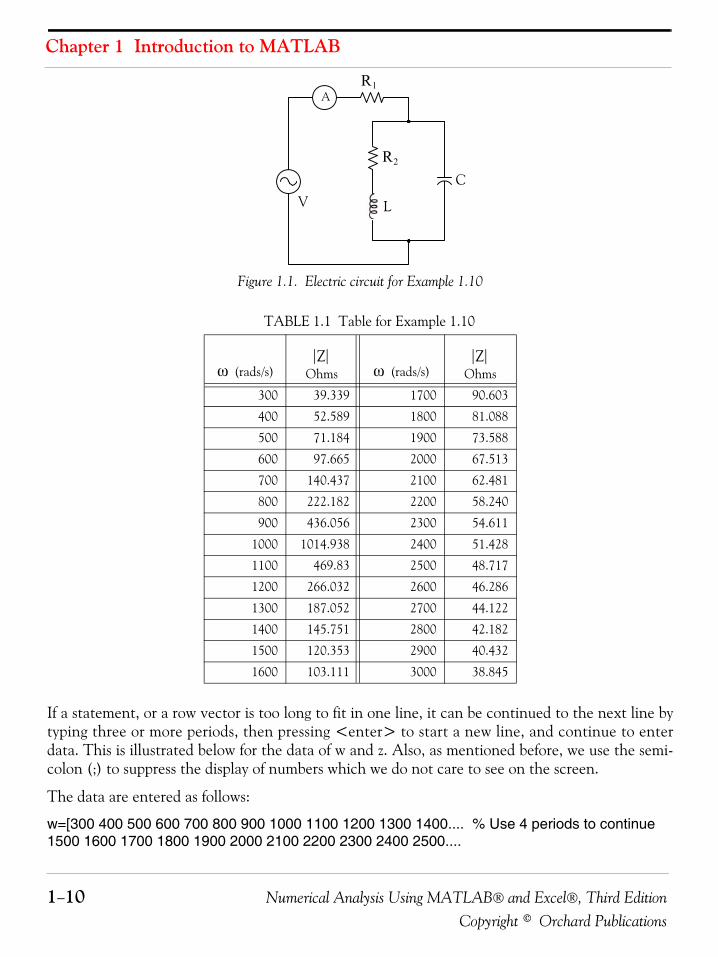
Consider the electric circuit of Figure 1.1, where the radian frequency (radians/second) of theapplied voltage was varied from to in steps of radians/second, while the amplitudewas held constant. The ammeter readings were then recorded for each frequency. The magnitudeof the impedance was computed as and the data were tabulated in Table 1.1.
Plot the magnitude of the impedance, that is, versus radian frequency .
Solution:
We cannot type (omega) in the MATLAB command window, so we will use the English letterw instead.
x2 bx c+ + 0= x1 x2
b x x1 x2+( )– b=
c x1 x2⋅ c= b
c
y x x y
ω300 3000 100
Z Z V A⁄=
Z ω
ω
Chapter 1 Introduction to MATLAB
1−10 Numerical Analysis Using MATLAB® and Excel®, Third EditionCopyright © Orchard Publications
Figure 1.1. Electric circuit for Example 1.10
If a statement, or a row vector is too long to fit in one line, it can be continued to the next line bytyping three or more periods, then pressing <enter> to start a new line, and continue to enterdata. This is illustrated below for the data of w and z. Also, as mentioned before, we use the semi-colon (;) to suppress the display of numbers which we do not care to see on the screen.
The data are entered as follows:
w=[300 400 500 600 700 800 900 1000 1100 1200 1300 1400.... % Use 4 periods to continue1500 1600 1700 1800 1900 2000 2100 2200 2300 2400 2500....
TABLE 1.1 Table for Example 1.10
(rads/s)
Ohms (rads/s)
Ohms
300 39.339 1700 90.603
400 52.589 1800 81.088
500 71.184 1900 73.588
600 97.665 2000 67.513
700 140.437 2100 62.481
800 222.182 2200 58.240
900 436.056 2300 54.611
1000 1014.938 2400 51.428
1100 469.83 2500 48.717
1200 266.032 2600 46.286
1300 187.052 2700 44.122
1400 145.751 2800 42.182
1500 120.353 2900 40.432
1600 103.111 3000 38.845
A
V L
C
R2
R1
ωZ
ωZ
Numerical Analysis Using MATLAB® and Excel®, Third Edition 1−11Copyright © Orchard Publications
Using MATLAB to Make Plots
2600 2700 2800 2900 3000]; % Use semicolon to suppress display of these numbers%z=[39.339 52.789 71.104 97.665 140.437 222.182 436.056.... 1014.938 469.830 266.032 187.052 145.751 120.353 103.111.... 90.603 81.088 73.588 67.513 62.481 58.240 54.611 51.468.... 48.717 46.286 44.122 42.182 40.432 38.845];
Of course, if we want to see the values of w or z or both, we simply type w or z, and we press<enter>.
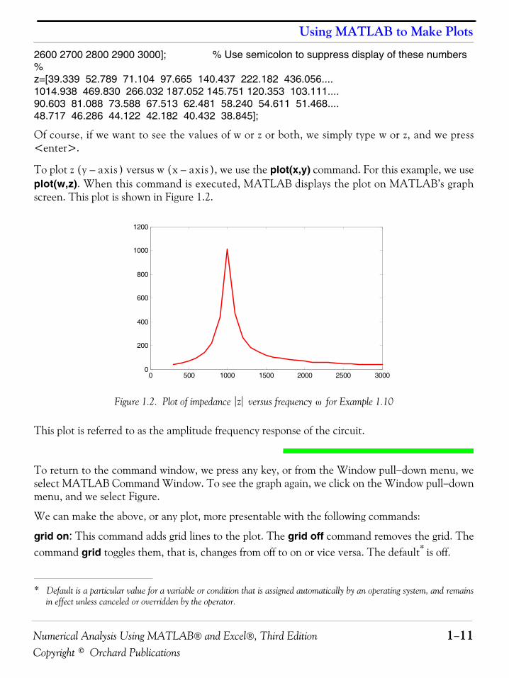
To plot z ( ) versus w ( ), we use the plot(x,y) command. For this example, we useplot(w,z). When this command is executed, MATLAB displays the plot on MATLAB’s graphscreen. This plot is shown in Figure 1.2.
Figure 1.2. Plot of impedance versus frequency for Example 1.10
This plot is referred to as the amplitude frequency response of the circuit.
To return to the command window, we press any key, or from the Window pull−down menu, weselect MATLAB Command Window. To see the graph again, we click on the Window pull−downmenu, and we select Figure.
We can make the above, or any plot, more presentable with the following commands:
grid on: This command adds grid lines to the plot. The grid off command removes the grid. Thecommand grid toggles them, that is, changes from off to on or vice versa. The default* is off.
* Default is a particular value for a variable or condition that is assigned automatically by an operating system, and remainsin effect unless canceled or overridden by the operator.
y axis– x axis–
0 500 1000 1500 2000 2500 30000
200
400
600
800
1000
1200
z ω
Chapter 1 Introduction to MATLAB
1−12 Numerical Analysis Using MATLAB® and Excel®, Third EditionCopyright © Orchard Publications
box off: This command removes the box (the solid lines which enclose the plot), and box onrestores the box. The command box toggles them. The default is on.
title(‘string’): This command adds a line of the text string (label) at the top of the plot.
xlabel(‘string’) and ylabel(‘string’) are used to label the − and −axis respectively.
The amplitude frequency response is usually represented with the −axis in a logarithmic scale.We can use the semilogx(x,y) command that is similar to the plot(x,y) command, except that the
−axis is represented as a log scale, and the −axis as a linear scale. Likewise, the semilogy(x,y)command is similar to the plot(x,y) command, except that the −axis is represented as a log scale,and the −axis as a linear scale. The loglog(x,y) command uses logarithmic scales for both axes.
Throughout this text, it will be understood that log is the common (base 10) logarithm, and ln isthe natural (base e) logarithm. We must remember, however, the function log(x) in MATLAB isthe natural logarithm, whereas the common logarithm is expressed as log10(x). Likewise, the loga-rithm to the base 2 is expressed as log2(x).
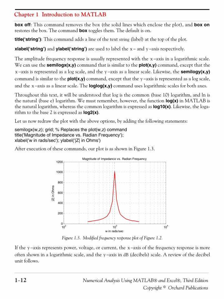
Let us now redraw the plot with the above options, by adding the following statements:
semilogx(w,z); grid; % Replaces the plot(w,z) commandtitle('Magnitude of Impedance vs. Radian Frequency');xlabel('w in rads/sec'); ylabel('|Z| in Ohms')
After execution of these commands, our plot is as shown in Figure 1.3.
Figure 1.3. Modified frequency response plot of Figure 1.2.
If the −axis represents power, voltage, or current, the −axis of the frequency response is moreoften shown in a logarithmic scale, and the −axis in dB (decibels) scale. A review of the decibelunit follows.
x y
x
x yy
x
102 103 1040
200
400
600
800
1000
1200Magnitude of Impedance vs. Radian Frequency
w in rads/sec
|Z| i
n O
hms
y xy
Numerical Analysis Using MATLAB® and Excel®, Third Edition 1−13Copyright © Orchard Publications
Using MATLAB to Make Plots
The ratio of any two values of the same quantity (power, voltage, or current) can be expressed indecibels (dB). Thus, we say that an amplifier has power gain, or a transmission line has apower loss of (or gain ). If the gain (or loss) is the output is equal to the input.By definition,
(1.10)
Therefore,
represents a power ratio of
represents a power ratio of
It is very useful to remember that:
represents a power ratio of
represents a power ratio of
represents a power ratio of
Also,
represents a power ratio of approximately
represents a power ratio of approximately
represents a power ratio of approximately
From these, we can estimate other values. For instance,
and since and
then,
Likewise, and this is equivalent to a power ratio of approximately
Using the relations
and
if we let , the dB values for voltage and current ratios become
10 dB7 dB 7– dB 0 dB
dB 10 Pout
Pin----------log=
10 dB 10
10n dB 10n
20 dB 100
30 dB 1 000,
60 dB 1 000 000, ,
1 dB 1.25
3 dB 2
7 dB 5
4 dB 3 dB 1 dB+= 3 dB power ratio of 2≅ 1 dB power ratio of 1.25≅
4 dB ratio of 2 1.25×( )≅ ratio of 2.5=
27 dB 20 dB 7 dB+=100 5× 500=
y x2log 2 xlog= =
P V 2
Z------- I 2Z= =
Z 1=
Chapter 1 Introduction to MATLAB
1−14 Numerical Analysis Using MATLAB® and Excel®, Third EditionCopyright © Orchard Publications
(1.11)
and
(1.12)
To display the voltage in a dB scale on the , we add the relation dB=20*log10(v), and wereplace the semilogx(w,z) command with semilogx(w,dB).
The command gtext(‘string’) switches to the current Figure Window, and displays a cross−hairwhich can be moved around with the mouse. For instance, we can use the commandgtext(‘Impedance |Z| versus Frequency’), and this will place a cross−hair in the Figure window.Then, using the mouse, we can move the cross−hair to the position where we want our label tobegin, and we press <enter>.
The command text(x,y,’string’) is similar to gtext(‘string’). It places a label on a plot in some spe-cific location specified by x and y, and string is the label which we want to place at that location.We will illustrate its use with the following example which plots a 3−phase sinusoidal waveform.
The first line of the script below has the form
linspace(first_value, last_value, number_of_values)
This command specifies the number of data points but not the increments between data points. Analternate command uses the colon notation and has the format
x=first: increment: last
This format specifies the increments between points but not the number of data points.
The script for the 3−phase plot is as follows:
x=linspace(0, 2*pi, 60); % pi is a built−in function in MATLAB;% we could have used x=0:0.02*pi:2*pi or x = (0: 0.02: 2)*pi instead;y=sin(x); u=sin(x+2*pi/3); v=sin(x+4*pi/3); plot(x,y,x,u,x,v); % The x−axis must be specified for each functiongrid on, box on, % turn grid and axes box ontext(0.75, 0.65, 'sin(x)'); text(2.85, 0.65, 'sin(x+2*pi/3)'); text(4.95, 0.65, 'sin(x+4*pi/3)')
These three waveforms are shown on the same plot of Figure 1.4.
In our previous examples, we did not specify line styles, markers, and colors for our plots. However,MATLAB allows us to specify various line types, plot symbols, and colors. These, or a combinationof these, can be added with the plot(x,y,s) command, where s is a character string containing one ormore characters shown on the three columns of Table 1.2.
MATLAB has no default color; it starts with blue and cycles through the first seven colors listed inTable 1.2 for each additional line in the plot. Also, there is no default marker; no markers are
dBv 10 Vout
Vin----------
2log 20 Vout
Vin----------log= =
dBi 10 Iout
Iin--------
2log 20 Iout
Iin--------log= =
v y axis–

Numerical Analysis Using MATLAB® and Excel®, Third Edition 1−15Copyright © Orchard Publications
Using MATLAB to Make Plots
drawn unless they are selected. The default line is the solid line.
Figure 1.4. Three−phase waveforms
For example, the command plot(x,y,'m*:') plots a magenta dotted line with a star at each datapoint, and plot(x,y,'rs') plots a red square at each data point, but does not draw any line becauseno line was selected. If we want to connect the data points with a solid line, we must typeplot(x,y,'rs−'). For additional information we can type help plot in MATLAB’s command screen.
TABLE 1.2 Styles, colors, and markets used in MATLAB
Symbol Color Symbol Marker Symbol Line Style
b blue . point − solid line
g green o circle : dotted line
r red x x−mark −. dash−dot line
c cyan + plus −− dashed line
m magenta * star
y yellow s square
k black d diamond
w white ⁄ triangle down
Ÿ triangle up
< triangle left
> triangle right
p pentagram
h hexagram
0 1 2 3 4 5 6 7-1
-0.5
0
0.5
1
sin(x) sin(x+2*pi/3) sin(x+4*pi/3)
Chapter 1 Introduction to MATLAB
1−16 Numerical Analysis Using MATLAB® and Excel®, Third EditionCopyright © Orchard Publications
The plots which we have discussed thus far are two−dimensional, that is, they are drawn on twoaxes. MATLAB has also a three−dimensional (three−axes) capability and this is discussed next.
The command plot3(x,y,z) plots a line in 3−space through the points whose coordinates are theelements of , , and , where , , and are three vectors of the same length.
The general format is plot3(x1,y1,z1,s1,x2,y2,z2,s2,x3,y3,z3,s3,...) where xn, yn, and zn are vectorsor matrices, and sn are strings specifying color, marker symbol, or line style. These strings are thesame as those of the two−dimensional plots.
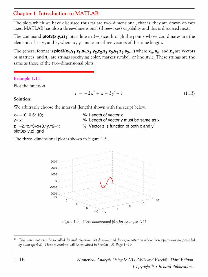
Example 1.11 Plot the function
(1.13)Solution:
We arbitrarily choose the interval (length) shown with the script below.
x= −10: 0.5: 10; % Length of vector x y= x; % Length of vector y must be same as xz= −2.*x.^3+x+3.*y.^2−1; % Vector z is function of both x and y*
plot3(x,y,z); grid
The three−dimensional plot is shown in Figure 1.5.
Figure 1.5. Three dimensional plot for Example 1.11
* This statement uses the so called dot multiplication, dot division, and dot exponentiation where these operations are precededby a dot (period). These operations will be explained in Section 1.8, Page 1−19.
x y z x y z
z 2x3– x 3y2 1–+ +=
-10-5
05
10
-10-5
05
10-2000
-1000
0
1000
2000
3000
Numerical Analysis Using MATLAB® and Excel®, Third Edition 1−17Copyright © Orchard Publications
Using MATLAB to Make Plots
The command plot3(x,y,z,'bd−') will display the plot in blue diamonds, connected with a solidline.
In a three−dimensional plot, we can use the zlabel(‘string’) command in addition to the xla-bel(‘string’) and ylabel(‘string’).
In a two−dimensional plot, we can set the limits of the − and − axes with the axis([xminxmax ymin ymax]) command. Likewise, in a three−dimensional plot we can set the limits of allthree axes with the axis([xmin xmax ymin ymax zmin zmax]) command. It must be placedafter the plot(x,y) or plot3(x,y,z) commands, or on the same line without first executing the plotcommand. This must be done for each plot. The three−dimensional text(x,y,z,’string’) commandwill place string beginning at the co−ordinate ( ) on the plot.
For three−dimensional plots, grid on and box off are the default states.
The mesh(x,y,z) command displays a three−dimensional plot. Another command, contour(Z,n),draws contour lines for n levels. We can also use the mesh(x,y,z) command with two vector argu-m en t s . Th e s e m u s t b e d e f i n e d a s a n d w h e r e
. In this case, the vertices of the mesh lines are the triples .We observe that x corresponds to the columns of , and y corresponds to the rows of .
To produce a mesh plot of a function of two variables, say , we must first generate the and matrices which consist of repeated rows and columns over the range of the variables
and . We can generate the matrices and with the [X,Y]=meshgrid(x,y) function whichcreates the matrix whose rows are copies of the vector x, and the matrix whose columns arecopies of the vector y.
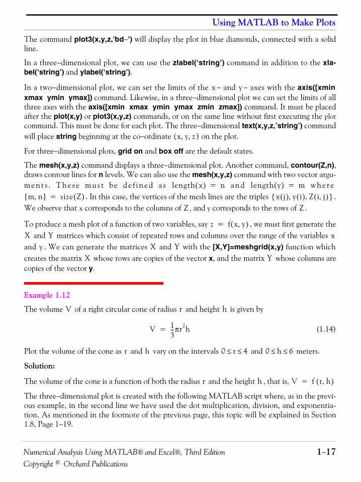
Example 1.12
The volume of a right circular cone of radius and height is given by
(1.14)
Plot the volume of the cone as and vary on the intervals and meters.
Solution:
The volume of the cone is a function of both the radius and the height , that is,
The three−dimensional plot is created with the following MATLAB script where, as in the previ-ous example, in the second line we have used the dot multiplication, division, and exponentia-tion. As mentioned in the footnote of the previous page, this topic will be explained in Section1.8, Page 1−19.
x y
x y z, ,
length x( ) n= length y( ) m=m n,[ ] size Z( )= x j( ) y i( ) Z i j,( ),,{ }
Z Z
z f x y,( )=X Y x
y X YX Y
V r h
V 13--πr2h=
r h 0 r 4≤ ≤ 0 h 6≤ ≤
r h V f r h,( )=
Chapter 1 Introduction to MATLAB
1−18 Numerical Analysis Using MATLAB® and Excel®, Third EditionCopyright © Orchard Publications
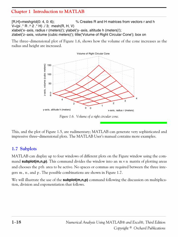
[R,H]=meshgrid(0: 4, 0: 6); % Creates R and H matrices from vectors r and hV=(pi .* R .^ 2 .* H) ./ 3; mesh(R, H, V)xlabel('x−axis, radius r (meters)'); ylabel('y−axis, altitude h (meters)');zlabel('z−axis, volume (cubic meters)'); title('Volume of Right Circular Cone'); box on
The three−dimensional plot of Figure 1.6, shows how the volume of the cone increases as theradius and height are increased.
Figure 1.6. Volume of a right circular cone.
This, and the plot of Figure 1.5, are rudimentary; MATLAB can generate very sophisticated andimpressive three−dimensional plots. The MATLAB User’s manual contains more examples.
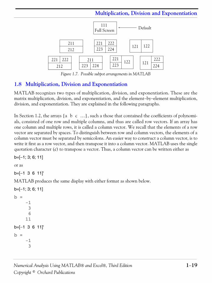
1.7 SubplotsMATLAB can display up to four windows of different plots on the Figure window using the com-mand subplot(m,n,p). This command divides the window into an matrix of plotting areasand chooses the area to be active. No spaces or commas are required between the three inte-gers , , and . The possible combinations are shown in Figure 1.7.
We will illustrate the use of the subplot(m,n,p) command following the discussion on multiplica-tion, division and exponentiation that follows.
01
23
4
0
2
4
60
50
100
150
x-axis, radius r (meters)
Volume of Right Circular Cone
y-axis, altitude h (meters)
z-ax
is,
volu
me
(cub
ic m
eter
s)
m n×pth
m n p
Numerical Analysis Using MATLAB® and Excel®, Third Edition 1−19Copyright © Orchard Publications
Multiplication, Division and Exponentiation
Figure 1.7. Possible subpot arrangements in MATLAB
1.8 Multiplication, Division and ExponentiationMATLAB recognizes two types of multiplication, division, and exponentiation. These are thematrix multiplication, division, and exponentiation, and the element−by−element multiplication,division, and exponentiation. They are explained in the following paragraphs.
In Section 1.2, the arrays , such a those that contained the coefficients of polynomi-als, consisted of one row and multiple columns, and thus are called row vectors. If an array hasone column and multiple rows, it is called a column vector. We recall that the elements of a rowvector are separated by spaces. To distinguish between row and column vectors, the elements of acolumn vector must be separated by semicolons. An easier way to construct a column vector, is towrite it first as a row vector, and then transpose it into a column vector. MATLAB uses the singlequotation character (¢) to transpose a vector. Thus, a column vector can be written either as
b=[−1; 3; 6; 11]
or as
b=[−1 3 6 11]'
MATLAB produces the same display with either format as shown below.
b=[−1; 3; 6; 11]
b = -1 3 6 11
b=[−1 3 6 11]'
b = -1 3
111Full Screen Default
211 212
221 222 223 224
121 122
221 222 212
211 223 224
221 223
122 121 222224
a b c …[ ]
Chapter 1 Introduction to MATLAB
1−20 Numerical Analysis Using MATLAB® and Excel®, Third EditionCopyright © Orchard Publications
6 11
We will now define Matrix Multiplication and Element−by−Element multiplication.
1. Matrix Multiplication (multiplication of row by column vectors)
Let
and
be two vectors. We observe that is defined as a row vector whereas is defined as a columnvector, as indicated by the transpose operator (′). Here, multiplication of the row vector bythe column vector , is performed with the matrix multiplication operator (*). Then,
(B.15)
For example, if
and
the matrix multiplication produces the single value 68, that is,
and this is verified with the MATLAB script
A=[1 2 3 4 5]; B=[ −2 6 −3 8 7]'; A*B % Observe transpose operator (‘) in B
ans =
68
Now, let us suppose that both and are row vectors, and we attempt to perform a row−by−row multiplication with the following MATLAB statements.
A=[1 2 3 4 5]; B=[−2 6 −3 8 7]; A*B % No transpose operator (‘) here
When these statements are executed, MATLAB displays the following message:
??? Error using ==> *
Inner matrix dimensions must agree.
Here, because we have used the matrix multiplication operator (*) in A*B, MATLAB expects
A a1 a2 a3 … an[ ]=
B b1 b2 b3 … bn[ ]'=
A BA
B
A*B a1b1 a2b2 a3b3 … anbn+ + + +[ ] gle valuesin= =
A 1 2 3 4 5[ ]=
B 2– 6 3– 8 7[ ]'=
A*B
A∗B 1 2–( ) 2 6 3 3–( ) 4 8 5 7×+×+×+×+× 68= =
A B
Numerical Analysis Using MATLAB® and Excel®, Third Edition 1−21Copyright © Orchard Publications
Multiplication, Division and Exponentiation
vector to be a column vector, not a row vector. It recognizes that is a row vector, andwarns us that we cannot perform this multiplication using the matrix multiplication operator(*). Accordingly, we must perform this type of multiplication with a different operator. Thisoperator is defined below.
2. Element−by−Element Multiplication (multiplication of a row vector by another row vector)
Let
and
be two row vectors. Here, multiplication of the row vector by the row vector is per-formed with the dot multiplication operator (.*). There is no space between the dot and themultiplication symbol. Thus,
(B.16)
This product is another row vector with the same number of elements, as the elements of and .
As an example, let
and
Dot multiplication of these two row vectors produce the following result.
Check with MATLAB:
C=[1 2 3 4 5]; % Vectors C and D must haveD=[−2 6 −3 8 7]; % same number of elementsC.*D % We observe that this is a dot multiplication
ans = -2 12 -9 32 35
Similarly, the division (/) and exponentiation (^) operators, are used for matrix division andexponentiation, whereas dot division (./) and dot exponentiation (.^) are used for element−by−element division and exponentiation, as illustrated with the examples above.
We must remember that no space is allowed between the dot (.) and the multiplication (*),division ( /), and exponentiation (^) operators.
Note: A dot (.) is never required with the plus (+) and minus (−) operators.
B B
C c1 c2 c3 … cn[ ]=
D d1 d2 d3 … dn[ ]=
C D
C.∗D c1d1 c2d2 c3d3 … cndn[ ]=
CD
C 1 2 3 4 5[ ]=
D 2– 6 3– 8 7[ ]=
C.∗D 1 2–( )× 2 6× 3 3–( )× 4 8 5 7×× 2– 12 9– 32 35= =
Chapter 1 Introduction to MATLAB
1−22 Numerical Analysis Using MATLAB® and Excel®, Third EditionCopyright © Orchard Publications
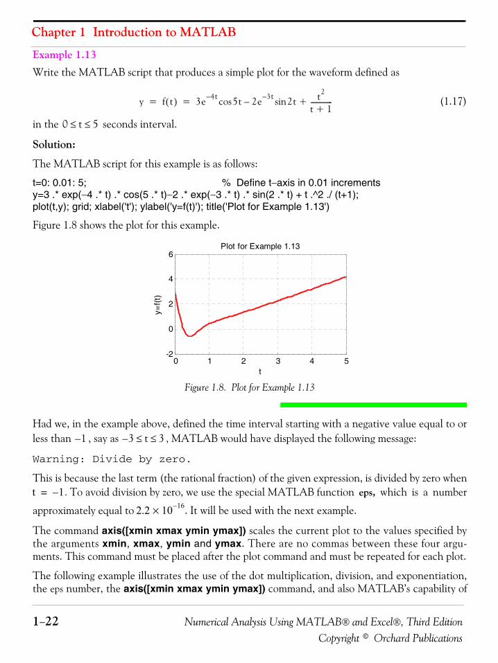
Example 1.13 Write the MATLAB script that produces a simple plot for the waveform defined as
(1.17)
in the seconds interval.
Solution:
The MATLAB script for this example is as follows:
t=0: 0.01: 5; % Define t−axis in 0.01 incrementsy=3 .* exp(−4 .* t) .* cos(5 .* t)−2 .* exp(−3 .* t) .* sin(2 .* t) + t .^2 ./ (t+1);plot(t,y); grid; xlabel('t'); ylabel('y=f(t)'); title('Plot for Example 1.13')
Figure 1.8 shows the plot for this example.
Figure 1.8. Plot for Example 1.13
Had we, in the example above, defined the time interval starting with a negative value equal to orless than , say as , MATLAB would have displayed the following message:
Warning: Divide by zero.
This is because the last term (the rational fraction) of the given expression, is divided by zero when. To avoid division by zero, we use the special MATLAB function eps, which is a number
approximately equal to . It will be used with the next example.
The command axis([xmin xmax ymin ymax]) scales the current plot to the values specified bythe arguments xmin, xmax, ymin and ymax. There are no commas between these four argu-ments. This command must be placed after the plot command and must be repeated for each plot.
The following example illustrates the use of the dot multiplication, division, and exponentiation,the eps number, the axis([xmin xmax ymin ymax]) command, and also MATLAB’s capability of
y f t( ) 3e 4t– 5tcos 2e 3t– 2tsin– t2
t 1+-------------+= =
0 t 5≤ ≤
0 1 2 3 4 5-2
0
2
4
6
t
y=f(t
)
Plot for Example 1.13
1– 3 t 3≤ ≤–
t 1–=
2.2 10 16–×
Numerical Analysis Using MATLAB® and Excel®, Third Edition 1−23Copyright © Orchard Publications
Multiplication, Division and Exponentiation
displaying up to four windows of different plots.
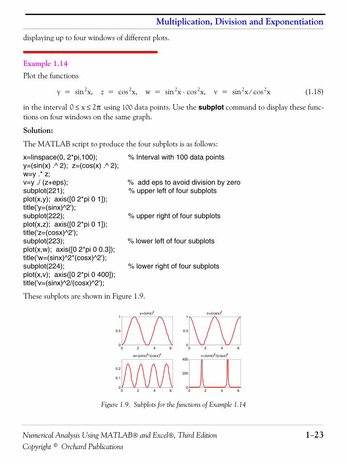
Example 1.14 Plot the functions
(1.18)
in the interval using 100 data points. Use the subplot command to display these func-tions on four windows on the same graph.
Solution:
The MATLAB script to produce the four subplots is as follows:
x=linspace(0, 2*pi,100); % Interval with 100 data pointsy=(sin(x) .^ 2); z=(cos(x) .^ 2); w=y .* z;v=y ./ (z+eps); % add eps to avoid division by zerosubplot(221); % upper left of four subplotsplot(x,y); axis([0 2*pi 0 1]);title('y=(sinx)^2');subplot(222); % upper right of four subplotsplot(x,z); axis([0 2*pi 0 1]); title('z=(cosx)^2');subplot(223); % lower left of four subplotsplot(x,w); axis([0 2*pi 0 0.3]);title('w=(sinx)^2*(cosx)^2');subplot(224); % lower right of four subplotsplot(x,v); axis([0 2*pi 0 400]);title('v=(sinx)^2/(cosx)^2');
These subplots are shown in Figure 1.9.
Figure 1.9. Subplots for the functions of Example 1.14
y x2sin z, x2cos w, x2sin x2cos⋅ v, x2sin x2cos⁄= = = =
0 x 2π≤ ≤
0 2 4 60
0.5
1y=(sinx)2
0 2 4 60
0.5
1z=(cosx)2
0 2 4 60
0.1
0.2
w=(sinx)2*(cosx)2
0 2 4 60
200
400v=(sinx)2/(cosx)2
Chapter 1 Introduction to MATLAB
1−24 Numerical Analysis Using MATLAB® and Excel®, Third EditionCopyright © Orchard Publications
The next example illustrates MATLAB’s capabilities with imaginary numbers. We will introducethe real(z) and imag(z) functions which display the real and imaginary parts of the complex quan-tity z = x + iy, the abs(z), and the angle(z) functions that compute the absolute value (magni-tude) and phase angle of the complex quantity . We will also use thepolar(theta,r) function that produces a plot in polar coordinates, where r is the magnitude, thetais the angle in radians, and the round(n) function that rounds a number to its nearest integer.
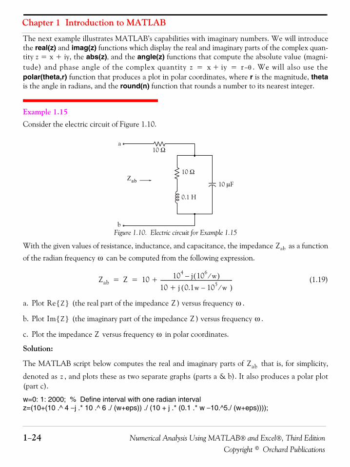
Example 1.15 Consider the electric circuit of Figure 1.10.
Figure 1.10. Electric circuit for Example 1.15
With the given values of resistance, inductance, and capacitance, the impedance as a function
of the radian frequency can be computed from the following expression.
(1.19)
a. Plot (the real part of the impedance ) versus frequency .
b. Plot (the imaginary part of the impedance ) versus frequency .
c. Plot the impedance versus frequency in polar coordinates.
Solution:
The MATLAB script below computes the real and imaginary parts of that is, for simplicity,
denoted as , and plots these as two separate graphs (parts a & b). It also produces a polar plot(part c).
w=0: 1: 2000; % Define interval with one radian intervalz=(10+(10 .^ 4 −j .* 10 .^ 6 ./ (w+eps)) ./ (10 + j .* (0.1 .* w −10.^5./ (w+eps))));
z x iy+ r θ–= =
a
b
10 Ω
10 Ω
0.1 H
10 μFZab
Zab
ω
Zab Z 10 104 j 106 w⁄( )–
10 j 0.1w 105 w⁄ –( )+--------------------------------------------------------+= =
Re Z{ } Z ω
Im Z{ } Z ω
Z ω
Zab
z
Numerical Analysis Using MATLAB® and Excel®, Third Edition 1−25Copyright © Orchard Publications
Multiplication, Division and Exponentiation
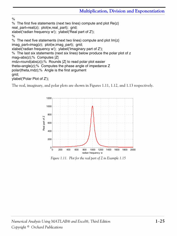
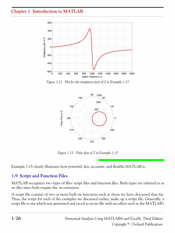
%% The first five statements (next two lines) compute and plot Re{z}real_part=real(z); plot(w,real_part); grid;xlabel('radian frequency w'); ylabel('Real part of Z');%% The next five statements (next two lines) compute and plot Im{z}imag_part=imag(z); plot(w,imag_part); grid;xlabel('radian frequency w'); ylabel('Imaginary part of Z');% The last six statements (next six lines) below produce the polar plot of zmag=abs(z);% Computes |Z|rndz=round(abs(z));% Rounds |Z| to read polar plot easiertheta=angle(z);% Computes the phase angle of impedance Zpolar(theta,rndz);% Angle is the first argumentgrid;ylabel('Polar Plot of Z');
The real, imaginary, and polar plots are shown in Figures 1.11, 1.12, and 1.13 respectively.
Figure 1.11. Plot for the real part of Z in Example 1.15
0 200 400 600 800 1000 1200 1400 1600 1800 20000
200
400
600
800
1000
1200
radian frequency w
Rea
l par
t of
Z
Chapter 1 Introduction to MATLAB
1−26 Numerical Analysis Using MATLAB® and Excel®, Third EditionCopyright © Orchard Publications
Figure 1.12. Plot for the imaginary part of Z in Example 1.15
Figure 1.13. Polar plot of Z in Example 1.15
Example 1.15 clearly illustrates how powerful, fast, accurate, and flexible MATLAB is.
1.9 Script and Function FilesMATLAB recognizes two types of files: script files and function files. Both types are referred to asm−files since both require the .m extension.
A script file consists of two or more built−in functions such as those we have discussed thus far.Thus, the script for each of the examples we discussed earlier, make up a script file. Generally, ascript file is one which was generated and saved as an m−file with an editor such as the MATLAB’s
0 200 400 600 800 1000 1200 1400 1600 1800 2000-600
-400
-200
0
200
400
600
radian frequency w
Imag
inar
y pa
rt o
f Z
500
1000
1500
30
210
60
240
90
270
120
300
150
330
180 0
Pol
ar P
lot o
f Z
Numerical Analysis Using MATLAB® and Excel®, Third Edition 1−27Copyright © Orchard Publications
Script and Function Files
Editor/Debugger.
A function file is a user−defined function using MATLAB. We use function files for repetitivetasks. The first line of a function file must contain the word function, followed by the output argu-ment, the equal sign ( = ), and the input argument enclosed in parentheses. The function nameand file name must be the same, but the file name must have the extension .m. For example, thefunction file consisting of the two lines below
function y = myfunction(x)y=x .^ 3 + cos(3 .* x)
is a function file and must be saved. To save it, from the File menu of the command window, wechoose New and click on M−File. This takes us to the Editor Window where we type these twolines and we save it as myfunction.m.
We will use the following MATLAB functions with the next example.
The function fzero(f,x) tries to find a zero of a function of one variable, where f is a string con-taining the name of a real−valued function of a single real variable. MATLAB searches for a valuenear a point where the function f changes sign, and returns that value, or returns NaN if thesearch fails.
Important: We must remember that we use roots(p) to find the roots of polynomials only, such asthose in Examples 1.1 and 1.2.
fplot(fcn,lims) − plots the function specified by the string fcn between the x−axis limits specifiedby lims = [xmin xmax]. Using lims = [xmin xmax ymin ymax] also controls the y−axis limits.The string fcn must be the name of an m−file function or a string with variable .
NaN (Not−a−Number) is not a function; it is MATLAB’s response to an undefined expressionsuch as , , or inability to produce a result as described on the next paragraph. We canavoid division by zero using the eps number, which we mentioned earlier.
Example 1.16 Find the zeros, maxima and minima of the function
(1.20)
in the interval
Solution:We first plot this function to observe the approximate zeros, maxima, and minima using the fol-lowing script:
x
0 0⁄ ∞ ∞⁄
f x( ) 1x 0.1–( )2 0.01+
------------------------------------------ 1x 1.2–( )2 0.04+
------------------------------------------ 10–+=
1.5 x 1.5≤ ≤–
Chapter 1 Introduction to MATLAB
1−28 Numerical Analysis Using MATLAB® and Excel®, Third EditionCopyright © Orchard Publications
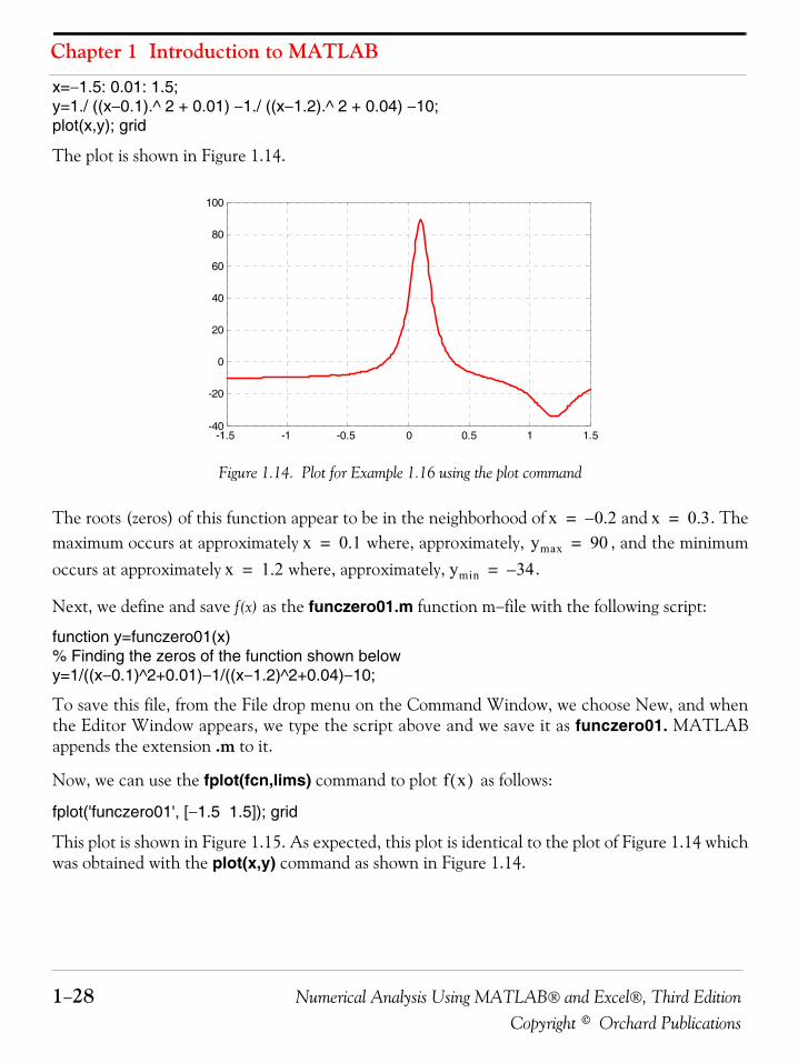
x=−1.5: 0.01: 1.5;y=1./ ((x−0.1).^ 2 + 0.01) −1./ ((x−1.2).^ 2 + 0.04) −10;plot(x,y); grid
The plot is shown in Figure 1.14.
Figure 1.14. Plot for Example 1.16 using the plot command
The roots (zeros) of this function appear to be in the neighborhood of and . Themaximum occurs at approximately where, approximately, , and the minimumoccurs at approximately where, approximately, .
Next, we define and save f(x) as the funczero01.m function m−file with the following script:
function y=funczero01(x)% Finding the zeros of the function shown belowy=1/((x−0.1)^2+0.01)−1/((x−1.2)^2+0.04)−10;
To save this file, from the File drop menu on the Command Window, we choose New, and whenthe Editor Window appears, we type the script above and we save it as funczero01. MATLABappends the extension .m to it.
Now, we can use the fplot(fcn,lims) command to plot as follows:
fplot('funczero01', [−1.5 1.5]); grid
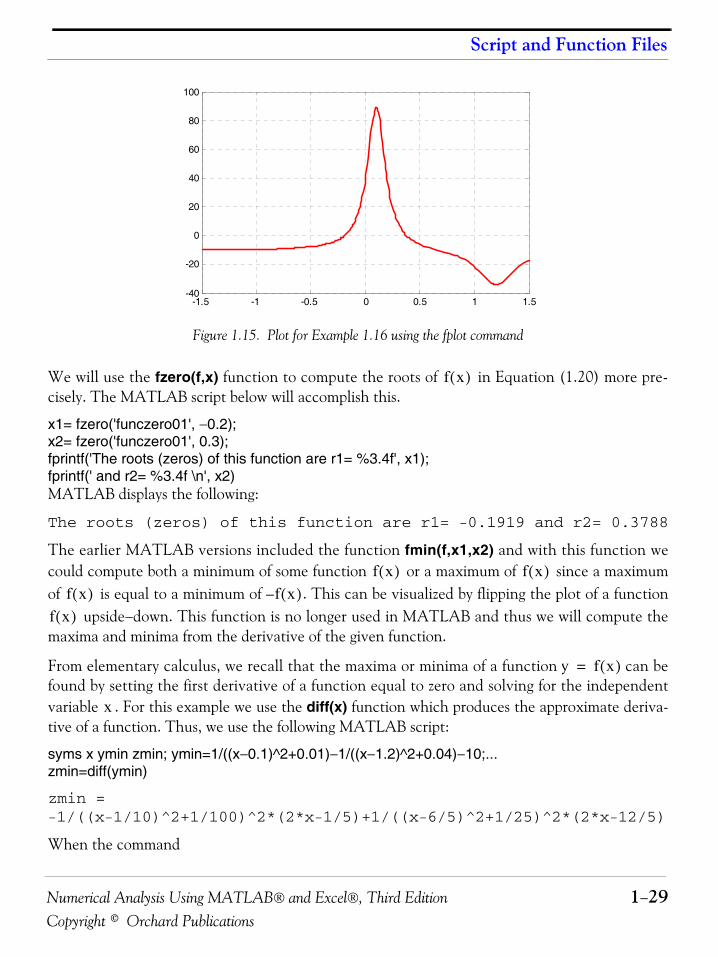
This plot is shown in Figure 1.15. As expected, this plot is identical to the plot of Figure 1.14 whichwas obtained with the plot(x,y) command as shown in Figure 1.14.
-1.5 -1 -0.5 0 0.5 1 1.5-40
-20
0
20
40
60
80
100
x 0.2–= x 0.3=x 0.1= ymax 90=
x 1.2= ymin 34–=
f x( )
Numerical Analysis Using MATLAB® and Excel®, Third Edition 1−29Copyright © Orchard Publications
Script and Function Files
Figure 1.15. Plot for Example 1.16 using the fplot command
We will use the fzero(f,x) function to compute the roots of in Equation (1.20) more pre-cisely. The MATLAB script below will accomplish this.
x1= fzero('funczero01', −0.2);x2= fzero('funczero01', 0.3);fprintf('The roots (zeros) of this function are r1= %3.4f', x1);fprintf(' and r2= %3.4f \n', x2)MATLAB displays the following:
The roots (zeros) of this function are r1= -0.1919 and r2= 0.3788
The earlier MATLAB versions included the function fmin(f,x1,x2) and with this function wecould compute both a minimum of some function or a maximum of since a maximumof is equal to a minimum of . This can be visualized by flipping the plot of a function
upside−down. This function is no longer used in MATLAB and thus we will compute themaxima and minima from the derivative of the given function.
From elementary calculus, we recall that the maxima or minima of a function can befound by setting the first derivative of a function equal to zero and solving for the independentvariable . For this example we use the diff(x) function which produces the approximate deriva-tive of a function. Thus, we use the following MATLAB script:
syms x ymin zmin; ymin=1/((x−0.1)^2+0.01)−1/((x−1.2)^2+0.04)−10;...zmin=diff(ymin)
zmin =-1/((x-1/10)^2+1/100)^2*(2*x-1/5)+1/((x-6/5)^2+1/25)^2*(2*x-12/5)
When the command
-1.5 -1 -0.5 0 0.5 1 1.5-40
-20
0
20
40
60
80
100
f x( )
f x( ) f x( )f x( ) f x( )–
f x( )
y f x( )=
x
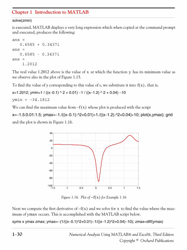
Chapter 1 Introduction to MATLAB
1−30 Numerical Analysis Using MATLAB® and Excel®, Third EditionCopyright © Orchard Publications
solve(zmin)
is executed, MATLAB displays a very long expression which when copied at the command promptand executed, produces the following:
ans = 0.6585 + 0.3437ians = 0.6585 - 0.3437ians = 1.2012
The real value above is the value of at which the function has its minimum value aswe observe also in the plot of Figure 1.15.
To find the value of y corresponding to this value of x, we substitute it into , that is,
x=1.2012; ymin=1 / ((x−0.1) ^ 2 + 0.01) −1 / ((x−1.2) ^ 2 + 0.04) −10
ymin = -34.1812
We can find the maximum value from whose plot is produced with the script
x=−1.5:0.01:1.5; ymax=−1./((x−0.1).^2+0.01)+1./((x−1.2).^2+0.04)+10; plot(x,ymax); grid
and the plot is shown in Figure 1.16.
Figure 1.16. Plot of for Example 1.16
Next we compute the first derivative of and we solve for to find the value where the max-imum of occurs. This is accomplished with the MATLAB script below.
syms x ymax zmax; ymax=−(1/((x−0.1)^2+0.01)−1/((x−1.2)^2+0.04)−10); zmax=diff(ymax)
1.2012 x y
f x( )
f x( )–
-1.5 -1 -0.5 0 0.5 1 1.5-100
-80
-60
-40
-20
0
20
40
f x( )–
f x( )– xymax
Numerical Analysis Using MATLAB® and Excel®, Third Edition 1−31Copyright © Orchard Publications
Display Formats
zmax = 1/((x-1/10)^2+1/100)^2*(2*x-1/5)-1/((x-6/5)^2+1/25)^2*(2*x-12/5)
solve(zmax)
When the command
solve(zmax)
is executed, MATLAB displays a very long expression which when copied at the commandprompt and executed, produces the following:
ans = 0.6585 + 0.3437i
ans = 0.6585 - 0.3437i
ans = 1.2012ans = 0.0999
From the values above we choose which is consistent with the plots of Figures 1.15and 1.16. Accordingly, we execute the following script to obtain the value of .
x=0.0999; % Using this value find the corresponding value of ymaxymax=1 / ((x−0.1) ^ 2 + 0.01) −1 / ((x−1.2) ^ 2 + 0.04) −10
ymax = 89.2000
1.10 Display FormatsMATLAB displays the results on the screen in integer format without decimals if the result is aninteger number, or in short floating point format with four decimals if it a fractional number. Theformat displayed has nothing to do with the accuracy in the computations. MATLAB performs allcomputations with accuracy up to 16 decimal places.The output format can changed with the format command. The available formats can be displayedwith the help format command as follows:
help format
FORMAT Set output format.All computations in MATLAB are done in double precision.FORMAT may be used to switch between different output displayformats as follows:
x 0.0999=ymin
Chapter 1 Introduction to MATLAB
1−32 Numerical Analysis Using MATLAB® and Excel®, Third EditionCopyright © Orchard Publications
FORMAT Default. Same as SHORT.FORMAT SHORT Scaled fixed point format with 5 digits.FORMAT LONG Scaled fixed point format with 15 digits.FORMAT SHORT E Floating point format with 5 digits.FORMAT LONG E Floating point format with 15 digits.FORMAT SHORT G Best of fixed or floating point format with 5 digits.FORMAT LONG G Best of fixed or floating point format with 15 digits.FORMAT HEX Hexadecimal format.FORMAT + The symbols +, - and blank are printed for positive, negative and zero elements. Imaginary parts are ignored.FORMAT BANK Fixed format for dollars and cents.FORMAT RAT Approximation by ratio of small integers.
Spacing:
FORMAT COMPACT Suppress extra line-feeds.FORMAT LOOSE Puts the extra line-feeds back in.
Some examples with different format displays age given below.
format short 33.3335 Four decimal digits (default)
format long 33.33333333333334 16 digits
format short e 3.3333e+01 Four decimal digits plus exponent
format short g 33.333 Better of format short or format short e
format bank 33.33 two decimal digits
format + only + or − or zero are printed
format rat 100/3 rational approximation
Numerical Analysis Using MATLAB® and Excel®, Third Edition 1−33Copyright © Orchard Publications
Summary
1.11 Summary• We can get help with MATLAB topics by typing help followed by any topic available. For
example, the command help matlab\iofun will display input/output information, and help mat-lab graphics will display help on graphics.
• The MATLAB Demos menu displays MATLAB’s capabilities. To access it, we type demo andwe see the different topics. Whenever we want to return to the command window, we click onthe Close button.
• We type quit or exit when we are done and want to leave MATLAB.
• We use the clear command if we want to clear all previous values, variables, and equationswithout exiting.
• The clc command clears the screen but MATLAB still remembers all values, variables andequations which we have already used.
• All text after the % (percent) symbol is interpreted by MATLAB as a comment line and thus itis ignored during the execution of a program. A comment can be typed on the same line as thefunction or command or as a separate line.
• For computations involving complex numbers we can use either , or to denote the imagi-nary part of the complex number.
• In MATLAB, a polynomial is expressed as a row vector of the form . The
elements of this vector are the coefficients of the polynomial in descending order. We mustinclude terms whose coefficients are zero.
• We find the roots of any polynomial with the roots(p) function where p is a row vector con-taining the polynomial coefficients in descending order.
• We can compute the coefficients of a polynomial from a given set of roots with the poly(r)function where r is a row vector containing the roots.
• The polyval(p,x) function evaluates a polynomial at some specified value of the inde-pendent variable .
• The conv(a,b) function multiplies the polynomials a and b.
• The [q,r]=deconv(c,d) function divides polynomial c by polynomial d and displays the quo-tient q and remainder r.
• The polyder(p) function produces the coefficients of the derivative of a polynomial p.
• We can write MATLAB statements in one line if we separate them by commas or semicolons.Commas will display the results whereas semicolons will suppress the display.
i j
an an 1– a2 a1 a0[ ]ai
p x( )x
Chapter 1 Introduction to MATLAB
1−34 Numerical Analysis Using MATLAB® and Excel®, Third EditionCopyright © Orchard Publications
• Rational Polynomials are those which can be expressed in ratio form, that is, as
where some of the terms in the numerator and/or denominator may be zero. Normally, weexpress the numerator and denominator of a rational function as a combination of linear andquadratic factors.
• We use the MATLAB command plot(x,y) to make two−dimensional plots. This commandplots versus where x is the horizontal axis (abscissa), and y is the vertical axis (ordinate).
• If a statement, or a row vector is too long to fit in one line, it can be continued to the next lineby typing three or more periods, then pressing <enter> to start a new line, and continue toenter data.
• We can make a two−dimensional plot more presentable with the commands grid, box,title(‘string’), xlabel(‘string’), and ylabel(‘string’). For a three−dimensional plot, we can alsouse the zlabel(‘string’) command.
• The semilogx(x,y) command is similar to the plot(x,y) command, except that the −axis isrepresented as a log scale, and the −axis as a linear scale. Likewise, the semilogy(x,y) com-mand is similar to the plot(x,y) command, except that the −axis is represented as a log scale,and the −axis as a linear scale. The loglog(x,y) command uses logarithmic scales for bothaxes.
• The function log(x) in MATLAB is the natural logarithm, whereas the common logarithm isexpressed as log10(x). Likewise, the logarithm to the base 2 is expressed as log2(x).
• The ratio of any two values of the same quantity, typically power, is normally expressed in deci-bels (dB) and by definition,
• The command gtext(‘string’) switches to the current Figure Window, and displays a cross−hairwhich can be moved around with the mouse. The command text(x,y,’string’) is similar togtext(‘string’); it places a label on a plot in some specific location specified by x and y, andstring is the label which we want to place at that location.
• The command linspace(first_value, last_value, number_of_values) specifies the number ofdata points but not the increments between data points. An alternate command uses the colonnotation and has the format x=first: increment: last. This format specifies the incrementsbetween points but not the number of data points.
R x( ) Num x( )Den x( )---------------------
bnxn bn 1– xn 1– bn 2– xn 2– … b1x b0+ + + + +
amxm am 1– xm 1– am 2– xm 2– … a1x a0+ + + + +-------------------------------------------------------------------------------------------------------------------------= =
y x
xy
yx
dB 10 Pout
Pin----------log=
Numerical Analysis Using MATLAB® and Excel®, Third Edition 1−35Copyright © Orchard Publications
Summary
• MATLAB has no default color; it starts with blue and cycles through seven colors. Also, thereis no default marker; no markers are drawn unless they are selected. The default line is thesolid line.
• The plot3(x,y,z) command plots a line in 3−space through the points whose coordinates arethe elements of , , and , where x, y, and z are three vectors of the same length.
• In a two−dimensional plot, we can set the limits of the − and −axes with the axis([xminxmax ymin ymax]) command. Likewise, in a three−dimensional plot we can set the limits ofall three axes with the axis([xmin xmax ymin ymax zmin zmax]) command. It must beplaced after the plot(x,y) or plot3(x,y,z) commands, or on the same line without first execut-ing the plot command. This must be done for each plot. The three−dimensionaltext(x,y,z,’string’) command will place string beginning at the co−ordinate ( ) on theplot.
• The mesh(x,y,z) command displays a three−dimensional plot. Another command, con-tour(Z,n), draws contour lines for n levels. We can also use the mesh(x,y,z) command withtwo vector arguments. These must be defined as and where . In this case, the vertices of the mesh lines are the triples
. We observe that x corresponds to the columns of , and y corresponds tothe rows of . To produce a mesh plot of a function of two variables, say , we mustfirst generate the and matrices which consist of repeated rows and columns over therange of the variables and . We can generate the matrices and with the [X,Y]=mesh-grid(x,y) function which creates the matrix whose rows are copies of the vector x, and thematrix whose columns are copies of the vector y.
• MATLAB can display up to four windows of different plots on the Figure window using thecommand subplot(m,n,p). This command divides the window into an matrix of plottingareas and chooses the area to be active.
• With MATLAB, matrix multiplication (multiplication of row by column vectors) is performedwith the matrix multiplication operator (*), whereas element−by−element multiplication isperformed with the dot multiplication operator (.*). Similarly, the division (/) and exponentia-tion (^) operators, are used for matrix division and exponentiation, whereas dot division (./)and dot exponentiation (.^) are used for element−by−element division and exponentiation.
• To avoid division by zero, we use the special MATLAB function eps, which is a number
approximately equal to .
• The command axis([xmin xmax ymin ymax]) scales the current plot to the values specifiedby the arguments xmin, xmax, ymin and ymax. There are no commas between these fourarguments. This command must be placed after the plot command and must be repeated foreach plot.
x y z
x y
x y z, ,
length x( ) n= length y( ) m=m n,[ ] size Z( )=
x j( ) y i( ) Z i j,( ),,{ } ZZ z f x y,( )=
X Yx y X Y
XY
m n×pth
2.2 10 16–×
Chapter 1 Introduction to MATLAB
1−36 Numerical Analysis Using MATLAB® and Excel®, Third EditionCopyright © Orchard Publications
• The real(z) and imag(z) functions display the real and imaginary parts of the complex quantityz = x + iy, and the abs(z), and the angle(z) functions compute the absolute value (magnitude)and phase angle of the complex quantity . The polar(theta,r) function pro-duces a plot in polar coordinates, where r is the magnitude, and theta is the angle in radians.
• MATLAB recognizes two types of files: script files and function files. Both types are referred toas m−files. A script file consists of two or more built−in functions. Generally, a script file is onewhich was generated and saved as an m−file with an editor such as the MATLAB’s Editor/Debugger. A function file is a user−defined function using MATLAB. We use function files forrepetitive tasks. The first line of a function file must contain the word function, followed by theoutput argument, the equal sign ( = ), and the input argument enclosed in parentheses. Thefunction name and file name must be the same, but the file name must have the extension .m.
• The MATLAB fmin(f,x1,x2) function minimizes a function of one variable. It attempts toreturn a value of where is minimum in the interval . The string f containsthe name of the function to be minimized.
• The MATLAB fplot(fcn,lims) command plots the function specified by the string fcn betweenthe −axis limits specified by lims = [xmin xmax]. Using lims = [xmin xmax ymin ymax] alsocontrols the −axis limits. The string fcn must be the name of an m−file function or a stringwith variable .
• The MATLAB fprintf(format,array) command used above displays and prints both text andarrays. It uses specifiers to indicate where and in which format the values would be displayedand printed. Thus, if %f is used, the values will be displayed and printed in fixed decimal for-mat, and if %e is used, the values will be displayed and printed in scientific notation format.With these commands only the real part of each parameter is processed.
• MATLAB displays the results on the screen in integer format without decimals if the result isan integer number, or in short floating point format with four decimals if it a fractional number.The format displayed has nothing to do with the accuracy in the computations. MATLAB per-forms all computations with accuracy up to 16 decimal places.
z x iy+ r θ–= =
x f x( ) x1 x x2< <
xyx
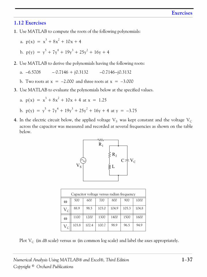
Numerical Analysis Using MATLAB® and Excel®, Third Edition 1−37Copyright © Orchard Publications
Exercises
1.12 Exercises1. Use MATLAB to compute the roots of the following polynomials:
a.
b.
2. Use MATLAB to derive the polynomials having the following roots:
a.
b. Two roots at and three roots at
3. Use MATLAB to evaluate the polynomials below at the specified values.
a. at
b. at
4. In the electric circuit below, the applied voltage was kept constant and the voltage across the capacitor was measured and recorded at several frequencies as shown on the tablebelow.
Plot (in dB scale) versus (in common log scale) and label the axes appropriately.
Capacitor voltage versus radian frequency
500 600 700 800 900 1000
88.9 98.5 103.0 104.9 105.3 104.8
1100 1200 1300 1400 1500 1600
103.8 102.4 100.7 98.9 96.5 94.9
p x( ) x3 8x2 10x 4+ + +=
p y( ) y5 7y4 19y3 25y2 16y 4+ + + + +=
6.5708– 0.7146– j0.3132+ 0.7146– j– 0.3132
x 2.000–= x 3.000–=
p x( ) x3 8x2 10x 4+ + += x 1.25=
p y( ) y5 7y4 19y3 25y2 16y 4+ + + + += y 3.75–=
VS VC
CVS
R1
R2VC
L
ω
VC
ω
VC
VC ω
Chapter 1 Introduction to MATLAB
1−38 Numerical Analysis Using MATLAB® and Excel®, Third EditionCopyright © Orchard Publications
1.13 Solutions to End−of−Chapter ExercisesDear Reader:
The remaining pages on this chapter contain the solutions to the exercises.
You must, for your benefit, make an honest effort to find the solutions to the exercises without firstlooking at the solutions that follow. It is recommended that first you go through and work outthose you feel that you know. For the exercises that you are uncertain, review this chapter and tryagain. Refer to the solutions as a last resort and rework those exercises at a later date.
You should follow this practice with the rest of the exercises of this book.
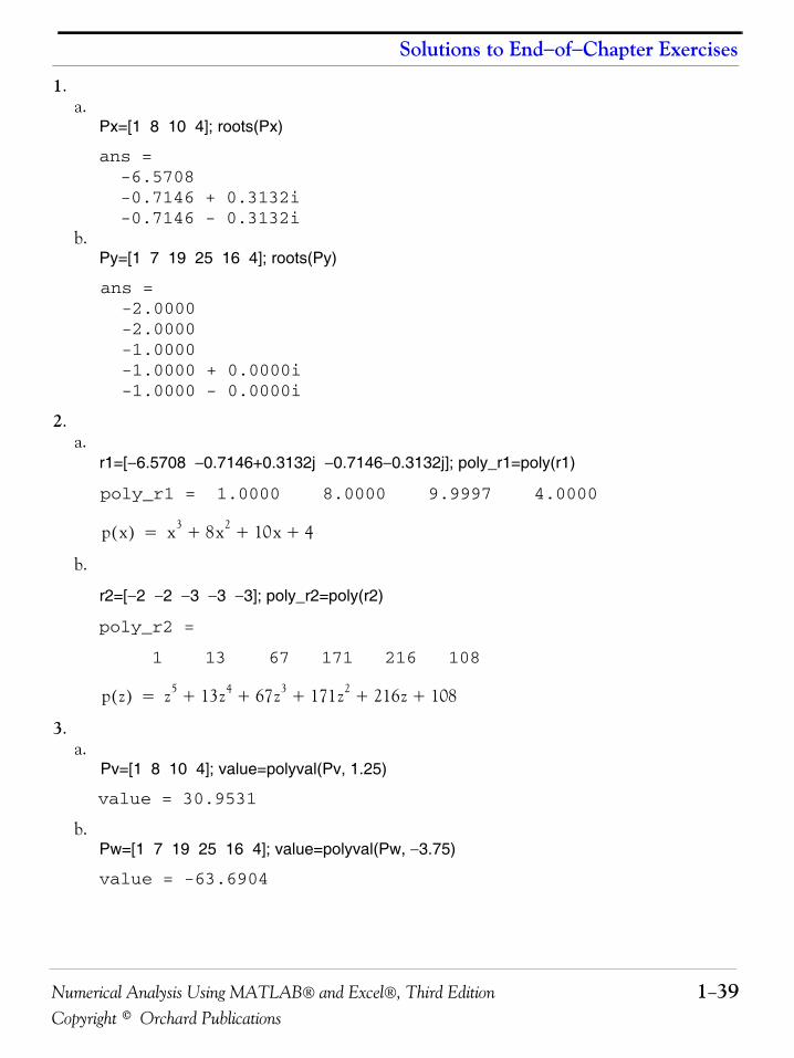
Numerical Analysis Using MATLAB® and Excel®, Third Edition 1−39Copyright © Orchard Publications
Solutions to End−of−Chapter Exercises
1.a.
Px=[1 8 10 4]; roots(Px)
ans = -6.5708 -0.7146 + 0.3132i -0.7146 - 0.3132i
b.Py=[1 7 19 25 16 4]; roots(Py)
ans = -2.0000 -2.0000 -1.0000 -1.0000 + 0.0000i -1.0000 - 0.0000i
2.a.
r1=[−6.5708 −0.7146+0.3132j −0.7146−0.3132j]; poly_r1=poly(r1)
poly_r1 = 1.0000 8.0000 9.9997 4.0000
b.
r2=[−2 −2 −3 −3 −3]; poly_r2=poly(r2)
poly_r2 =
1 13 67 171 216 108
3.a.
Pv=[1 8 10 4]; value=polyval(Pv, 1.25)
value = 30.9531
b.Pw=[1 7 19 25 16 4]; value=polyval(Pw, −3.75)
value = -63.6904
p x( ) x3 8x2 10x 4+ + +=
p z( ) z5 13z4 67z3 171z2 216z 108+ + + + +=
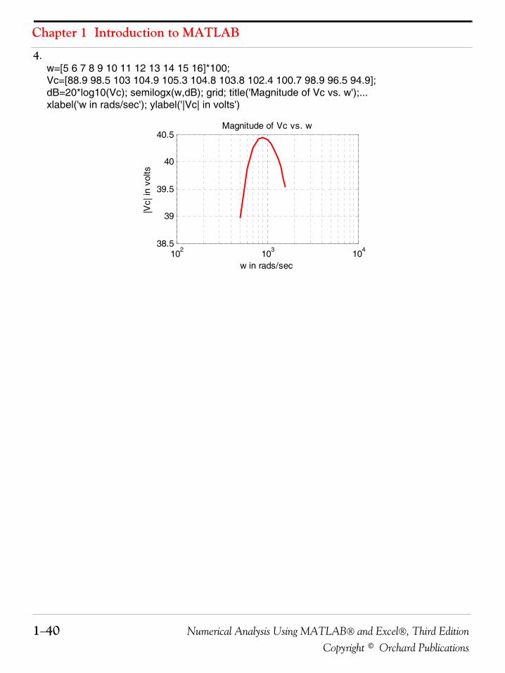
Chapter 1 Introduction to MATLAB
1−40 Numerical Analysis Using MATLAB® and Excel®, Third EditionCopyright © Orchard Publications
4.w=[5 6 7 8 9 10 11 12 13 14 15 16]*100;Vc=[88.9 98.5 103 104.9 105.3 104.8 103.8 102.4 100.7 98.9 96.5 94.9];dB=20*log10(Vc); semilogx(w,dB); grid; title('Magnitude of Vc vs. w');...xlabel('w in rads/sec'); ylabel('|Vc| in volts')
102 103 10438.5
39
39.5
40
40.5Magnitude of Vc vs. w
w in rads/sec
|Vc|
in v
olts
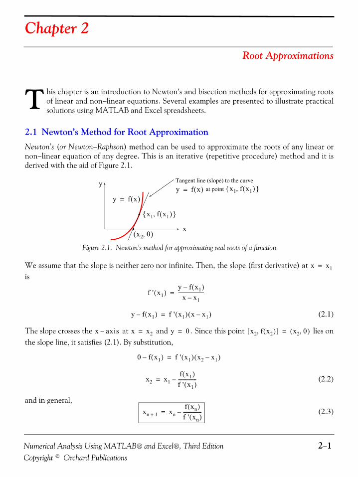
Numerical Analysis Using MATLAB® and Excel®, Third Edition 2−1Copyright © Orchard Publications
Chapter 2
Root Approximations
his chapter is an introduction to Newton’s and bisection methods for approximating rootsof linear and non−linear equations. Several examples are presented to illustrate practicalsolutions using MATLAB and Excel spreadsheets.
2.1 Newton’s Method for Root ApproximationNewton’s (or Newton−Raphson) method can be used to approximate the roots of any linear ornon−linear equation of any degree. This is an iterative (repetitive procedure) method and it isderived with the aid of Figure 2.1.
Figure 2.1. Newton’s method for approximating real roots of a function
We assume that the slope is neither zero nor infinite. Then, the slope (first derivative) at is
(2.1)
The slope crosses the at and . Since this point lies onthe slope line, it satisfies (2.1). By substitution,
(2.2)
and in general, (2.3)
T
•
•
Tangent line (slope) to the curve at point
y f x( )=
x
yx1 f x1( ),{ }
x2 0,( )
x1 f x1( ),{ }
y f x( )=
x x1=
f ' x1( )y f x1( )–
x x1–--------------------- =
y f x1( )– f ' x1( ) x x1–( )=
x axis– x x2= y 0= x2 f x2( ),[ ] x2 0,( )=
0 f x1( )– f ' x1( ) x2 x1–( )=
x2 x1f x1( )f ' x1( )---------------–=
xn 1+ xnf xn( )f ' xn( )---------------–=
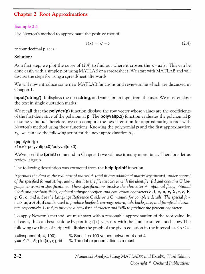
Chapter 2 Root Approximations
2−2 Numerical Analysis Using MATLAB® and Excel®, Third EditionCopyright © Orchard Publications
Example 2.1 Use Newton’s method to approximate the positive root of
(2.4)to four decimal places.
Solution:
As a first step, we plot the curve of (2.4) to find out where it crosses the . This can bedone easily with a simple plot using MATLAB or a spreadsheet. We start with MATLAB and willdiscuss the steps for using a spreadsheet afterwards.
We will now introduce some new MATLAB functions and review some which are discussed inChapter 1.
input(‘string’): It displays the text string, and waits for an input from the user. We must enclosethe text in single quotation marks.
We recall that the polyder(p) function displays the row vector whose values are the coefficientsof the first derivative of the polynomial p. The polyval(p,x) function evaluates the polynomial pat some value x. Therefore, we can compute the next iteration for approximating a root withNewton’s method using these functions. Knowing the polynomial p and the first approximation
, we can use the following script for the next approximation .
q=polyder(p)x1=x0−polyval(p,x0)/polyval(q,x0)
We’ve used the fprintf command in Chapter 1; we will use it many more times. Therefore, let usreview it again.
The following description was extracted from the help fprintf function.
It formats the data in the real part of matrix A (and in any additional matrix arguments), under controlof the specified format string, and writes it to the file associated with file identifier fid and contains C lan-guage conversion specifications. These specifications involve the character %, optional flags, optionalwidth and precision fields, optional subtype specifier, and conversion characters d, i, o, u, x, X, f, e, E,g, G, c, and s. See the Language Reference Guide or a C manual for complete details. The special for-mats \n,\r,\t,\b,\f can be used to produce linefeed, carriage return, tab, backspace, and formfeed charac-ters respectively. Use \\ to produce a backslash character and %% to produce the percent character.
To apply Newton’s method, we must start with a reasonable approximation of the root value. Inall cases, this can best be done by plotting versus with the familiar statements below. Thefollowing two lines of script will display the graph of the given equation in the interval .
x=linspace(−4, 4, 100); % Specifies 100 values between -4 and 4y=x .^ 2 − 5; plot(x,y); grid % The dot exponentiation is a must
f x( ) x2 5–=
x axis–
x0 x1
f x( ) x4 x 4≤ ≤–
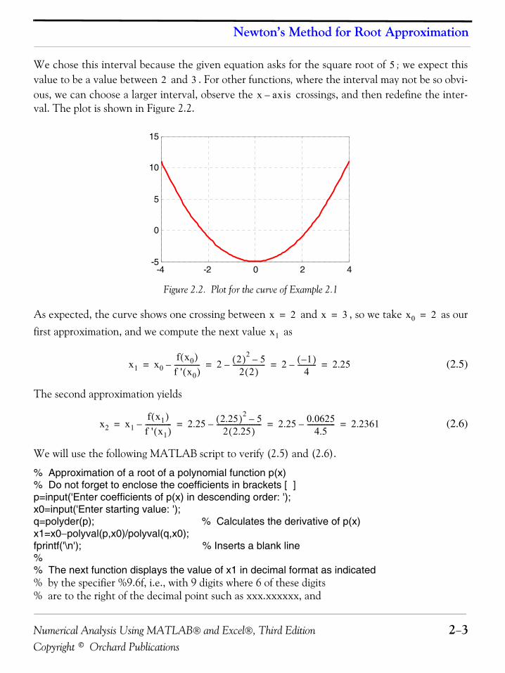
Numerical Analysis Using MATLAB® and Excel®, Third Edition 2−3Copyright © Orchard Publications
Newton’s Method for Root Approximation
We chose this interval because the given equation asks for the square root of ; we expect thisvalue to be a value between and . For other functions, where the interval may not be so obvi-ous, we can choose a larger interval, observe the crossings, and then redefine the inter-val. The plot is shown in Figure 2.2.
Figure 2.2. Plot for the curve of Example 2.1
As expected, the curve shows one crossing between and , so we take as ourfirst approximation, and we compute the next value as
(2.5)
The second approximation yields
(2.6)
We will use the following MATLAB script to verify (2.5) and (2.6).
% Approximation of a root of a polynomial function p(x)% Do not forget to enclose the coefficients in brackets [ ]p=input('Enter coefficients of p(x) in descending order: ');x0=input('Enter starting value: ');q=polyder(p); % Calculates the derivative of p(x)x1=x0−polyval(p,x0)/polyval(q,x0);fprintf('\n'); % Inserts a blank line%% The next function displays the value of x1 in decimal format as indicated % by the specifier %9.6f, i.e., with 9 digits where 6 of these digits% are to the right of the decimal point such as xxx.xxxxxx, and
52 3
x axis–
-4 -2 0 2 4-5
0
5
10
15
x 2= x 3= x0 2=
x1
x1 x0f x0( )f ' x0( )---------------– 2 2( )2 5–
2 2( )-------------------– 2 1–( )
4-----------– 2.25= = = =
x2 x1f x1( )f ' x1( )---------------– 2.25 2.25( )2 5–
2 2.25( )--------------------------– 2.25 0.0625
4.5----------------– 2.2361= = = =
Chapter 2 Root Approximations
2−4 Numerical Analysis Using MATLAB® and Excel®, Third EditionCopyright © Orchard Publications
% \n prints a blank line before printing x1fprintf('The next approximation is: %9.6f \n', x1)fprintf('\n'); % Inserts another blank line%fprintf('Rerun the program using this value as your next....approximation \n');
The following lines show MATLAB’s inquiries and our responses (inputs) for the first twoapproximations.
Enter coefficients of P(x) in descending order:[1 0 −5]Enter starting value: 2The next approximation is: 2.250000 Rerun the program using this value as yournext approximation Enter polynomial coefficients in descending order: [1 0 −5] Enter starting value: 2.25The next approximation is: 2.236111
We observe that this approximation is in close agreement with (2.6).
In Chapter 1 we discussed script files and function files. We recall that a function file is a user−defined function using MATLAB. We use function files for repetitive tasks. The first line of afunction file must contain the word function followed by the output argument, the equal sign (=),and the input argument enclosed in parentheses. The function name and file name must be thesame but the file name must have the extension .m. For example, the function file consisting ofthe two lines below
function y = myfunction(x)y=x .^ 3 + cos(3 .* x)
is a function file and must be saved as myfunction.m
We will use the while end loop, whose general form is
while expression commands ...endwhere the commands ... in the second line are executed as long as all elements in expression of thefirst line are true.
We will also be using the following commands:
Numerical Analysis Using MATLAB® and Excel®, Third Edition 2−5Copyright © Orchard Publications
Newton’s Method for Root Approximation
disp(x): Displays the array x without printing the array name. If x is a string, the text is displayed.For example, if , disp(v) displays 12, and disp(‘volts’) displays volts.
sprintf(format,A): Formats the data in the real part of matrix A under control of the specifiedformat string. For example,
sprintf('%d',round(pi))
ans =3
where the format script %d specifies an integer. Likewise,
sprintf('%4.3f',pi)
ans =3.142
where the format script %4.3f specifies a fixed format of 4 digits where 3 of these digits are allo-cated to the fractional part.
Example 2.2 Approximate one real root of the non−linear equation
(2.7)
to four decimal places using Newton’s method.
Solution:
As a first step, we sketch the curve to find out where the curve crosses the . We generatethe plot with the script below.
x=linspace(−pi, pi, 100); y=x .^ 2 + 4 .* x + 3 + sin(x) − x .* cos(x); plot(x,y); grid
The plot is shown in Figure 2.3.
The plot shows that one real root is approximately at , so we will use this value as our firstapproximation.
Next, we generate the function funcnewt01 and we save it as an m−file. To save it, from the Filemenu of the command window, we choose New and click on M−File. This takes us to the EditorWindow where we type the following three lines and we save it as funcnewt01.m.
function y=funcnewt01(x)% Approximating roots with Newton's methody=x .^ 2 + 4 .* x + 3 + sin(x) − x .* cos(x);
v 12=
f x( ) x2 4x 3 xsin x xcos–+ + +=
x axis–
x 1–=
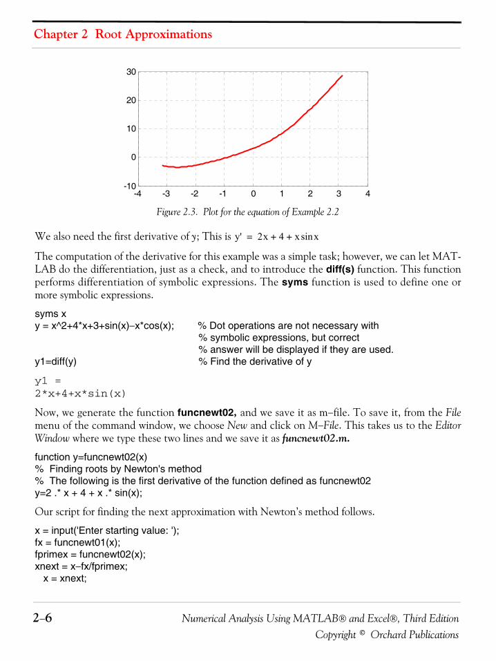
Chapter 2 Root Approximations
2−6 Numerical Analysis Using MATLAB® and Excel®, Third EditionCopyright © Orchard Publications
Figure 2.3. Plot for the equation of Example 2.2
We also need the first derivative of y; This is
The computation of the derivative for this example was a simple task; however, we can let MAT-LAB do the differentiation, just as a check, and to introduce the diff(s) function. This functionperforms differentiation of symbolic expressions. The syms function is used to define one ormore symbolic expressions.
syms xy = x^2+4*x+3+sin(x)−x*cos(x); % Dot operations are not necessary with
% symbolic expressions, but correct % answer will be displayed if they are used.
y1=diff(y) % Find the derivative of y
y1 =2*x+4+x*sin(x)
Now, we generate the function funcnewt02, and we save it as m−file. To save it, from the Filemenu of the command window, we choose New and click on M−File. This takes us to the EditorWindow where we type these two lines and we save it as funcnewt02.m.
function y=funcnewt02(x)% Finding roots by Newton's method% The following is the first derivative of the function defined as funcnewt02y=2 .* x + 4 + x .* sin(x);
Our script for finding the next approximation with Newton’s method follows.
x = input('Enter starting value: ');fx = funcnewt01(x);fprimex = funcnewt02(x);xnext = x−fx/fprimex; x = xnext;
-4 -3 -2 -1 0 1 2 3 4-10
0
10
20
30
y' 2x 4 x xsin+ +=
Numerical Analysis Using MATLAB® and Excel®, Third Edition 2−7Copyright © Orchard Publications
Approximations with Spreadsheets
fx = funcnewt01(x); fprimex = funcnewt02(x);disp(sprintf('First approximation is x = %9.6f \n', x))while input('Next approximation? (<enter>=no,1=yes)'); xnext=x−fx/fprimex; x=xnext; fx=funcnewt01(x); fprimex=funcnewt02(x);disp(sprintf('Next approximation is x = %9.6f \n', x)) end;disp(sprintf('%9.6f \n', x))
MATLAB produces the following result with as a starting value.
Enter starting value: −1 First approximation is: -0.894010 Next approximation? (<enter>=no,1=yes)1-0.895225Next approximation? (<enter>=no,1=yes) <enter>
We can also use the fzero(f,x) function. It was introduced in Chapter 1. This function tries tofind a zero of a function of one variable. The string f contains the name of a real−valued functionof a single real variable. As we recall, MATLAB searches for a value near a point where the func-tion f changes sign and returns that value, or returns NaN if the search fails.
2.2 Approximations with SpreadsheetsIn this section, we will go through several examples to illustrate the procedure of using a spread-sheet such as Excel* to approximate the real roots of linear and non−linear equations.
We recall that there is a standard procedure for finding the roots of a cubic equation; it isincluded here for convenience.
A cubic equation of the form
(2.8)can be reduced to the simpler form
(2.9)where
* We will illustrate our examples with Excel, although others such as Lotus 1−2−3, and Quattro can also be used. Hence-forth, all spreadsheet commands and formulas that we will be using, will be those of Excel.
1–
y3 py2 qy r+ + + 0=
x3 ax b+ + 0=
Chapter 2 Root Approximations
2−8 Numerical Analysis Using MATLAB® and Excel®, Third EditionCopyright © Orchard Publications
(2.10)
For the solution it is convenient to let
(2.11)
Then, the values of for which the cubic equation of (2.11) is equal to zero are
(2.12)
If the coefficients , , and are real, then (2.13)
While MATLAB handles complex numbers very well, spreadsheets do not. Therefore, unless weknow that the roots are all real, we should not use a spreadsheet to find the roots of a cubic equa-tion by substitution in the above formulas. However, we can use a spreadsheet to find the realroot since in any cubic equation there is at least one real root. For real roots, we can use a spread-sheet to define a range of values with small increments and compute the corresponding valuesof . Then, we can plot versus to observe the values of that make . Thisprocedure is illustrated with the examples that follow.
Note: In our subsequent discussion we will omit the word cell and the key <enter>. Thus B3,C11, and so on will be understood to be cell B3, cell C11, and so on. Also, after an entry has beenmade, it will be understood that the <enter> key was pressed.
Example 2.3 Compute the roots of the polynomial
(2.14)using Excel.
x y p3--- a+
13--- 3q p2–( ) b 1
27------ 2p3 9pq– 27r+( )= = =
A b–2
------ b2
4----- a3
27------++
3= B b–
2------ b2
4----- a3
27------++
3–=
x
x1 A B+= x2A B+
2--------------–
A B–2
-------------- 3–+= x3A B+
2--------------–
A B–2
-------------- 3––=
p q r
If b2
4----- a3
27------+ 0> one root will be real and the other two complex conjugates
If b2
4----- a3
27------+ 0< the roots will be real and unequal
If b2
4----- a3
27------+ 0= there will be three real roots with at least two equal
xy f x( )= y x x f x( ) 0=
y f x( ) x3 7x2– 16x 12–+= =
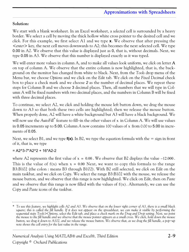
Numerical Analysis Using MATLAB® and Excel®, Third Edition 2−9Copyright © Orchard Publications
Approximations with Spreadsheets
Solution:
We start with a blank worksheet. In an Excel worksheet, a selected cell is surrounded by a heavyborder. We select a cell by moving the thick hollow white cross pointer to the desired cell and weclick. For this example, we first select A1 and we type x. We observe that after pressing the<enter> key, the next cell moves downwards to A2; this becomes the next selected cell. We type0.00 in A2. We observe that this value is displayed just as 0, that is, without decimals. Next, wetype 0.05 in A3. We observe that this number is displayed exactly as it was typed.
We will enter more values in column A, and to make all values look uniform, we click on letter Aon top of column A. We observe that the entire column is now highlighted, that is, the back-ground on the monitor has changed from white to black. Next, from the Tools drop menu of theMenu bar, we choose Options and we click on the Edit tab. We click on the Fixed Decimal checkbox to place a check mark and we choose 2 as the number of decimal places. We repeat thesesteps for Column B and we choose 3 decimal places. Then, all numbers that we will type in Col-umn A will be fixed numbers with two decimal places, and the numbers in Column B will be fixedwith three decimal places.
To continue, we select A2, we click and holding the mouse left button down, we drag the mousedown to A3 so that both these two cells are highlighted; then we release the mouse button.When properly done, A2 will have a white background but A3 will have a black background. Wewill now use the AutoFill* feature to fill−in the other values of in Column A. We will use valuesin 0.05 increments up to 5.00. Column A now contains 100 values of from 0.00 to 5.00 in incre-ments of 0.05.
Next, we select B1, and we type f(x). In B2, we type the equation formula with the = sign in frontof it, that is, we type
= A2^3-7*A2^2 + 16*A2-2
where A2 represents the first value of . We observe that B2 displays the value .This is the value of when Next, we want to copy this formula to the rangeB3:B102 (the colon : means B3 through B102). With B2 still selected, we click on Edit on themain taskbar, and we click on Copy. We select the range B3:B102 with the mouse, we release themouse button, and we observe that this range is now highlighted. We click on Edit, then on Pasteand we observe that this range is now filled with the values of . Alternately, we can use theCopy and Paste icons of the taskbar.
* To use this feature, we highlight cells A2 and A3. We observe that on the lower right corner of A3, there is a small blacksquare; this is called the fill handle. If it does not appear on the spreadsheet, we can make it visible by performing thesequential steps Tools>Options, select the Edit tab, and place a check mark on the Drag and Drop setting. Next, we pointthe mouse to the fill handle and we observe that the mouse pointer appears as a small cross. We click, hold down the mousebutton, we drag it down to A102, and we release the mouse button. We observe that, as we drag the fill handle, a pop−upnote shows the cell entry for the last value in the range.
xx
x 0.00= 12.000–
f x( ) x 0.00=
f x( )
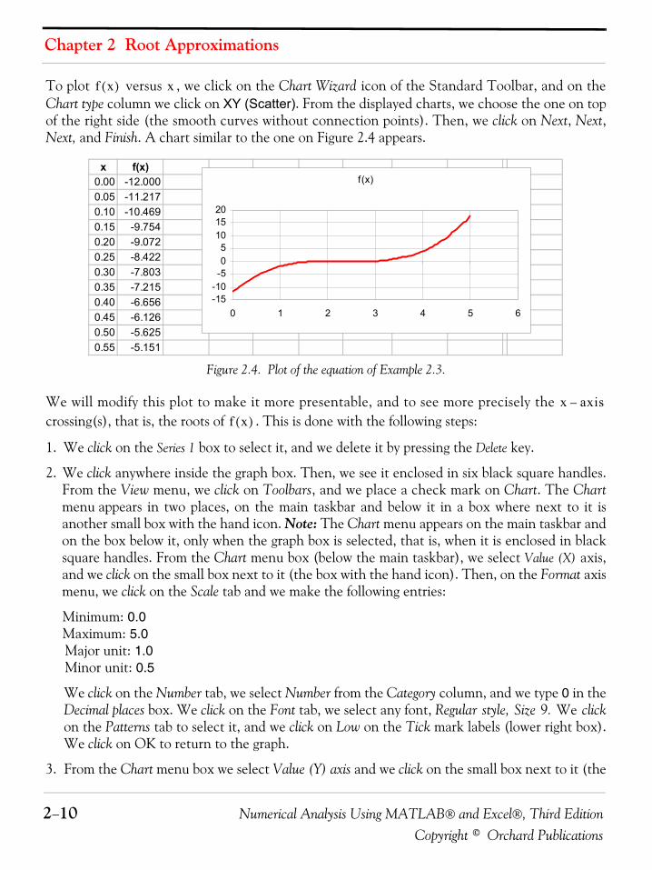
Chapter 2 Root Approximations
2−10 Numerical Analysis Using MATLAB® and Excel®, Third EditionCopyright © Orchard Publications
To plot versus , we click on the Chart Wizard icon of the Standard Toolbar, and on theChart type column we click on XY (Scatter). From the displayed charts, we choose the one on topof the right side (the smooth curves without connection points). Then, we click on Next, Next,Next, and Finish. A chart similar to the one on Figure 2.4 appears.
Figure 2.4. Plot of the equation of Example 2.3.
We will modify this plot to make it more presentable, and to see more precisely the crossing(s), that is, the roots of . This is done with the following steps:
1. We click on the Series 1 box to select it, and we delete it by pressing the Delete key.
2. We click anywhere inside the graph box. Then, we see it enclosed in six black square handles.From the View menu, we click on Toolbars, and we place a check mark on Chart. The Chartmenu appears in two places, on the main taskbar and below it in a box where next to it isanother small box with the hand icon. Note: The Chart menu appears on the main taskbar andon the box below it, only when the graph box is selected, that is, when it is enclosed in blacksquare handles. From the Chart menu box (below the main taskbar), we select Value (X) axis,and we click on the small box next to it (the box with the hand icon). Then, on the Format axismenu, we click on the Scale tab and we make the following entries:
Minimum: 0.0 Maximum: 5.0 Major unit: 1.0 Minor unit: 0.5
We click on the Number tab, we select Number from the Category column, and we type 0 in theDecimal places box. We click on the Font tab, we select any font, Regular style, Size 9. We clickon the Patterns tab to select it, and we click on Low on the Tick mark labels (lower right box).We click on OK to return to the graph.
3. From the Chart menu box we select Value (Y) axis and we click on the small box next to it (the
f x( ) x
x f(x)0.00 -12.0000.05 -11.2170.10 -10.4690.15 -9.7540.20 -9.0720.25 -8.4220.30 -7.8030.35 -7.2150.40 -6.6560.45 -6.1260.50 -5.6250.55 -5.151
f(x)
-15-10-505
101520
0 1 2 3 4 5 6
x axis–
f x( )
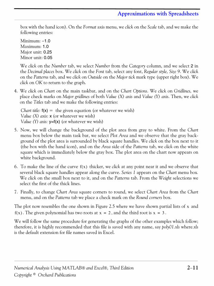
Numerical Analysis Using MATLAB® and Excel®, Third Edition 2−11Copyright © Orchard Publications
Approximations with Spreadsheets
box with the hand icon). On the Format axis menu, we click on the Scale tab, and we make thefollowing entries:
Minimum: −1.0Maximum: 1.0 Major unit: 0.25 Minor unit: 0.05
We click on the Number tab, we select Number from the Category column, and we select 2 inthe Decimal places box. We click on the Font tab, select any font, Regular style, Size 9. We clickon the Patterns tab, and we click on Outside on the Major tick mark type (upper right box). Weclick on OK to return to the graph.
4. We click on Chart on the main taskbar, and on the Chart Options. We click on Gridlines, weplace check marks on Major gridlines of both Value (X) axis and Value (Y) axis. Then, we clickon the Titles tab and we make the following entries:
Chart title: f(x) = the given equation (or whatever we wish)Value (X) axis: x (or whatever we wish)Value (Y) axis: y=f(x) (or whatever we wish)
5. Now, we will change the background of the plot area from gray to white. From the Chartmenu box below the main task bar, we select Plot Area and we observe that the gray back-ground of the plot area is surrounded by black square handles. We click on the box next to it(the box with the hand icon), and on the Area side of the Patterns tab, we click on the whitesquare which is immediately below the gray box. The plot area on the chart now appears onwhite background.
6. To make the line of the curve thicker, we click at any point near it and we observe thatseveral black square handles appear along the curve. Series 1 appears on the Chart menu box.We click on the small box next to it, and on the Patterns tab. From the Weight selections weselect the first of the thick lines.
7. Finally, to change Chart Area square corners to round, we select Chart Area from the Chartmenu, and on the Patterns tab we place a check mark on the Round corners box.
The plot now resembles the one shown in Figure 2.5 where we have shown partial lists of and. The given polynomial has two roots at , and the third root is .
We will follow the same procedure for generating the graphs of the other examples which follow;therefore, it is highly recommended that this file is saved with any name, say poly01.xls where.xlsis the default extension for file names saved in Excel.
f x( )
xf x( ) x 2= x 3=
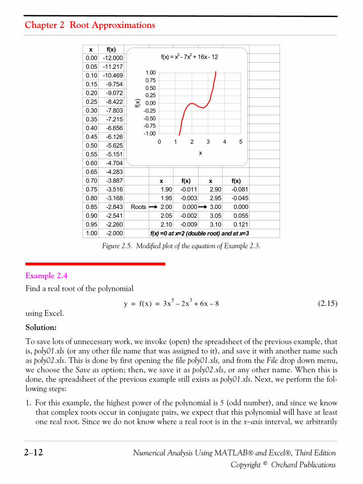
Chapter 2 Root Approximations
2−12 Numerical Analysis Using MATLAB® and Excel®, Third EditionCopyright © Orchard Publications
Figure 2.5. Modified plot of the equation of Example 2.3.
Example 2.4 Find a real root of the polynomial
(2.15)using Excel.
Solution:
To save lots of unnecessary work, we invoke (open) the spreadsheet of the previous example, thatis, poly01.xls (or any other file name that was assigned to it), and save it with another name suchas poly02.xls. This is done by first opening the file poly01.xls, and from the File drop down menu,we choose the Save as option; then, we save it as poly02.xls, or any other name. When this isdone, the spreadsheet of the previous example still exists as poly01.xls. Next, we perform the fol-lowing steps:
1. For this example, the highest power of the polynomial is 5 (odd number), and since we knowthat complex roots occur in conjugate pairs, we expect that this polynomial will have at leastone real root. Since we do not know where a real root is in the x−axis interval, we arbitrarily
x f(x)0.00 -12.0000.05 -11.2170.10 -10.4690.15 -9.7540.20 -9.0720.25 -8.4220.30 -7.8030.35 -7.2150.40 -6.6560.45 -6.1260.50 -5.6250.55 -5.1510.60 -4.7040.65 -4.2830.70 -3.887 x f(x) x f(x)0.75 -3.516 1.90 -0.011 2.90 -0.0810.80 -3.168 1.95 -0.003 2.95 -0.0450.85 -2.843 Roots 2.00 0.000 3.00 0.0000.90 -2.541 2.05 -0.002 3.05 0.0550.95 -2.260 2.10 -0.009 3.10 0.1211.00 -2.000 f(x) =0 at x=2 (double root) and at x=3
f(x) = x3 - 7x2 + 16x - 12
-1.00-0.75-0.50-0.250.000.250.500.751.00
0 1 2 3 4 5
x
f(x)
y f x( ) 3x5 2x3– 6x 8–+= =
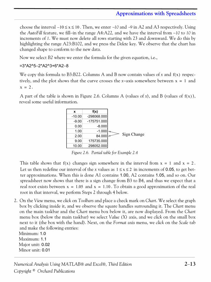
Numerical Analysis Using MATLAB® and Excel®, Third Edition 2−13Copyright © Orchard Publications
Approximations with Spreadsheets
choose the interval . Then, we enter −10 and −9 in A2 and A3 respectively. Usingthe AutoFill feature, we fill−in the range A4:A22, and we have the interval from −10 to 10 inincrements of 1. We must now delete all rows starting with 23 and downward. We do this byhighlighting the range A23:B102, and we press the Delete key. We observe that the chart haschanged shape to conform to the new data.
Now we select B2 where we enter the formula for the given equation, i.e.,
=3*A2^5−2*A2^3+6*A2−8
We copy this formula to B3:B22. Columns A and B now contain values of x and respec-tively, and the plot shows that the curve crosses the x−axis somewhere between and
.
A part of the table is shown in Figure 2.6. Columns A (values of x), and B (values of ),reveal some useful information.
Figure 2.6. Partial table for Example 2.4
This table shows that changes sign somewhere in the interval from and .Let us then redefine our interval of the x values as in increments of 0.05, to get bet-ter approximations. When this is done A1 contains 1.00, A2 contains 1.05, and so on. Ourspreadsheet now shows that there is a sign change from B3 to B4, and thus we expect that areal root exists between and . To obtain a good approximation of the realroot in that interval, we perform Steps 2 through 4 below.
2. On the View menu, we click on Toolbars and place a check mark on Chart. We select the graphbox by clicking inside it, and we observe the square handles surrounding it. The Chart menuon the main taskbar and the Chart menu box below it, are now displayed. From the Chartmenu box (below the main taskbar) we select Value (X) axis, and we click on the small boxnext to it (the box with the hand). Next, on the Format axis menu, we click on the Scale taband make the following entries:Minimum: 1.0Maximum: 1.1Major unit: 0.02Minor unit: 0.01
10 x 10≤ ≤–
f x( )x 1=
x 2=
f x( )
x f(x)-10.00 -298068.000-9.00 -175751.0000.00 -8.0001.00 -1.0002.00 84.0009.00 175735.000
10.00 298052.000
Sign Change
f x( ) x 1= x 2=
1 x 2≤ ≤
x 1.05= x 1.10=
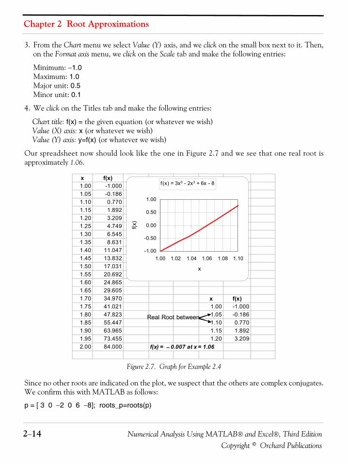
Chapter 2 Root Approximations
2−14 Numerical Analysis Using MATLAB® and Excel®, Third EditionCopyright © Orchard Publications
3. From the Chart menu we select Value (Y) axis, and we click on the small box next to it. Then,on the Format axis menu, we click on the Scale tab and make the following entries:
Minimum: −1.0Maximum: 1.0Major unit: 0.5Minor unit: 0.1
4. We click on the Titles tab and make the following entries:
Chart title: f(x) = the given equation (or whatever we wish)Value (X) axis: x (or whatever we wish)Value (Y) axis: y=f(x) (or whatever we wish)
Our spreadsheet now should look like the one in Figure 2.7 and we see that one real root isapproximately 1.06.
Figure 2.7. Graph for Example 2.4
Since no other roots are indicated on the plot, we suspect that the others are complex conjugates.We confirm this with MATLAB as follows:
p = [ 3 0 −2 0 6 −8]; roots_p=roots(p)
x f(x)1.00 -1.0001.05 -0.1861.10 0.7701.15 1.8921.20 3.2091.25 4.7491.30 6.5451.35 8.6311.40 11.0471.45 13.8321.50 17.0311.55 20.6921.60 24.8651.65 29.6051.70 34.970 x f(x)1.75 41.021 1.00 -1.0001.80 47.823 1.05 -0.1861.85 55.447 1.10 0.7701.90 63.965 1.15 1.8921.95 73.455 1.20 3.2092.00 84.000 f(x) = − 0.007 at x = 1.06
f (x) = 3x5 - 2x3 + 6x - 8
-1.00
-0.50
0.00
0.50
1.00
1.00 1.02 1.04 1.06 1.08 1.10
x
f(x)
Real Root between
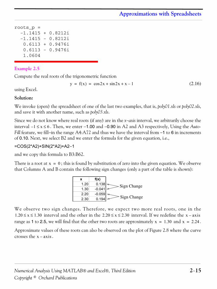
Numerical Analysis Using MATLAB® and Excel®, Third Edition 2−15Copyright © Orchard Publications
Approximations with Spreadsheets
roots_p = -1.1415 + 0.8212i -1.1415 - 0.8212i 0.6113 + 0.9476i 0.6113 - 0.9476i 1.0604
Example 2.5 Compute the real roots of the trigonometric function
(2.16)using Excel.
Solution:
We invoke (open) the spreadsheet of one of the last two examples, that is, poly01.xls or poly02.xls,and save it with another name, such as poly03.xls.
Since we do not know where real roots (if any) are in the x−axis interval, we arbitrarily choose theinterval . Then, we enter −1.00 and −0.90 in A2 and A3 respectively, Using the Auto-Fill feature, we fill−in the range A4:A72 and thus we have the interval from −1 to 6 in incrementsof 0.10. Next, we select B2 and we enter the formula for the given equation, i.e.,
=COS(2*A2)+SIN(2*A2)+A2−1
and we copy this formula to B3:B62.
There is a root at ; this is found by substitution of zero into the given equation. We observethat Columns A and B contain the following sign changes (only a part of the table is shown):
We observe two sign changes. Therefore, we expect two more real roots, one in the interval and the other in the interval. If we redefine the
range as 1 to 2.5, we will find that the other two roots are approximately and .
Approximate values of these roots can also be observed on the plot of Figure 2.8 where the curvecrosses the .
y f x( ) 2xcos 2x x+sin 1–+= =
1 x 6≤ ≤–
x 0=
x f(x)1.20 0.1381.30 -0.0412.20 -0.0592.30 0.194
Sign Change
Sign Change
1.20 x 1.30≤ ≤ 2.20 x 2.30≤ ≤ x axis–
x 1.30= x 2.24=
x axis–
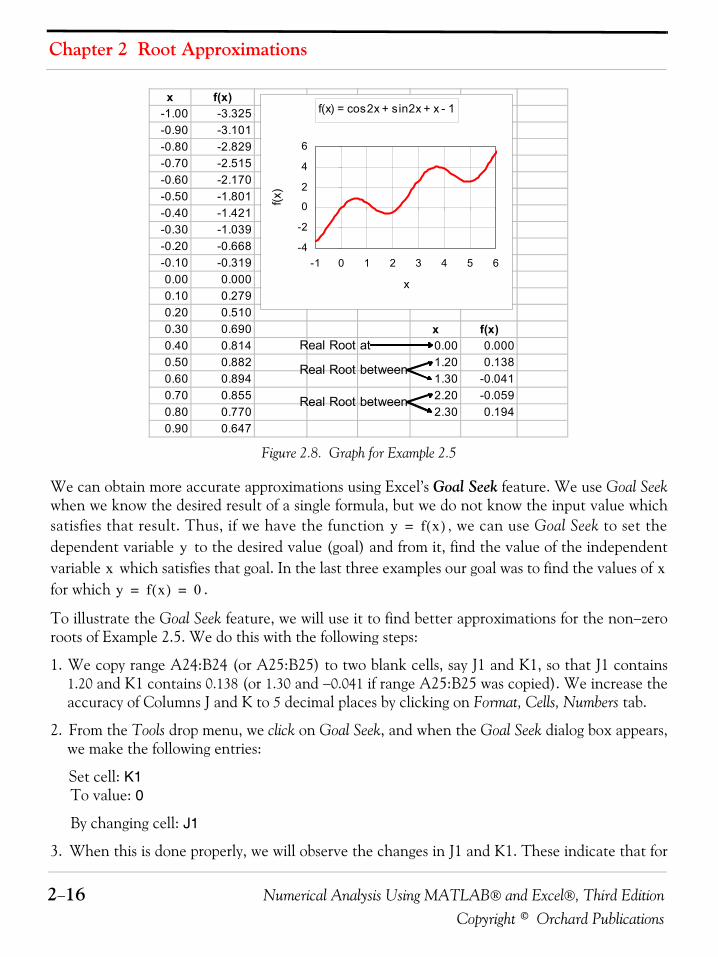
Chapter 2 Root Approximations
2−16 Numerical Analysis Using MATLAB® and Excel®, Third EditionCopyright © Orchard Publications
Figure 2.8. Graph for Example 2.5
We can obtain more accurate approximations using Excel’s Goal Seek feature. We use Goal Seekwhen we know the desired result of a single formula, but we do not know the input value whichsatisfies that result. Thus, if we have the function , we can use Goal Seek to set thedependent variable to the desired value (goal) and from it, find the value of the independentvariable which satisfies that goal. In the last three examples our goal was to find the values of for which .
To illustrate the Goal Seek feature, we will use it to find better approximations for the non−zeroroots of Example 2.5. We do this with the following steps:
1. We copy range A24:B24 (or A25:B25) to two blank cells, say J1 and K1, so that J1 contains1.20 and K1 contains 0.138 (or 1.30 and −0.041 if range A25:B25 was copied). We increase theaccuracy of Columns J and K to 5 decimal places by clicking on Format, Cells, Numbers tab.
2. From the Tools drop menu, we click on Goal Seek, and when the Goal Seek dialog box appears,we make the following entries:
Set cell: K1To value: 0
By changing cell: J1
3. When this is done properly, we will observe the changes in J1 and K1. These indicate that for
x f(x)-1.00 -3.325-0.90 -3.101-0.80 -2.829-0.70 -2.515-0.60 -2.170-0.50 -1.801-0.40 -1.421-0.30 -1.039-0.20 -0.668-0.10 -0.3190.00 0.0000.10 0.2790.20 0.5100.30 0.690 x f(x)0.40 0.814 0.00 0.0000.50 0.882 1.20 0.1380.60 0.894 1.30 -0.0410.70 0.855 2.20 -0.0590.80 0.770 2.30 0.1940.90 0.647
f(x) = cos2x + sin2x + x - 1
-4
-2
0
2
4
6
-1 0 1 2 3 4 5 6
xf(x
)
Real Root between
Real Root between
Real Root at
y f x( )=
yx x
y f x( ) 0= =
Numerical Analysis Using MATLAB® and Excel®, Third Edition 2−17Copyright © Orchard Publications
Approximations with Spreadsheets
, .
4. We repeat the above steps for the next root near , and we verify that for, .
Another method of using the Goal Seek feature, is with a chart such as those we’ve created for thelast three examples. We will illustrate the procedure with the chart of Example 2.5.
1. We point the mouse at the curve where it intersects the x−axis, near the point. Asquare box appears and displays Series 1, (1.30, −0.041). We observe that other points are alsodisplayed as the mouse is moved at different points near the curve.
2. We click anywhere near the curve, and we observe that five handles (black square boxes) aredisplayed along different points on the curve. Next, we click on the handle near the point, and when the cross symbol appears, we drag it towards the x−axis to change its value.The Goal Seek dialog box then appears where the Set cell shows B24. Then, in the To value boxwe enter 0, in the By changing cell we enter A24 and we click on OK. We observe now that A24displays 1.28 and B24 displays 0.000.
For repetitive tasks, such as finding the roots of polynomials, it is prudent to construct a template(model spreadsheet) with the appropriate formulas and then enter the coefficients of the polyno-mial to find its real roots*. This is illustrated with the next example.
Example 2.6 Construct a template (model spreadsheet), with Excel, which uses Newton’s method to approxi-mate a real root of any polynomial with real coefficients up to the seventh power; then, use it tocompute a root of the polynomial
(2.17)
given that one real root lies in the interval.
Solution:
1. We begin with a blank spreadsheet and we make the entries shown in Figure 2.9.
* There exists a numerical procedure, known as Bairstow’s method, that we can use to find the complex roots of a polyno-mial with real coefficients. We will not discuss this method here; it can be found in advanced numerical analysis textbooks.
x 1.27647= y f x( ) 0.00002= =
x 2.20=
x 2.22515= y f x( ) 0.00020= =
x 1.30=
x 1.30=
y f x( ) x7 6x6– 5x5 4x4– 3x3 2x2– x 15–+ + += =
4 x 6≤ ≤
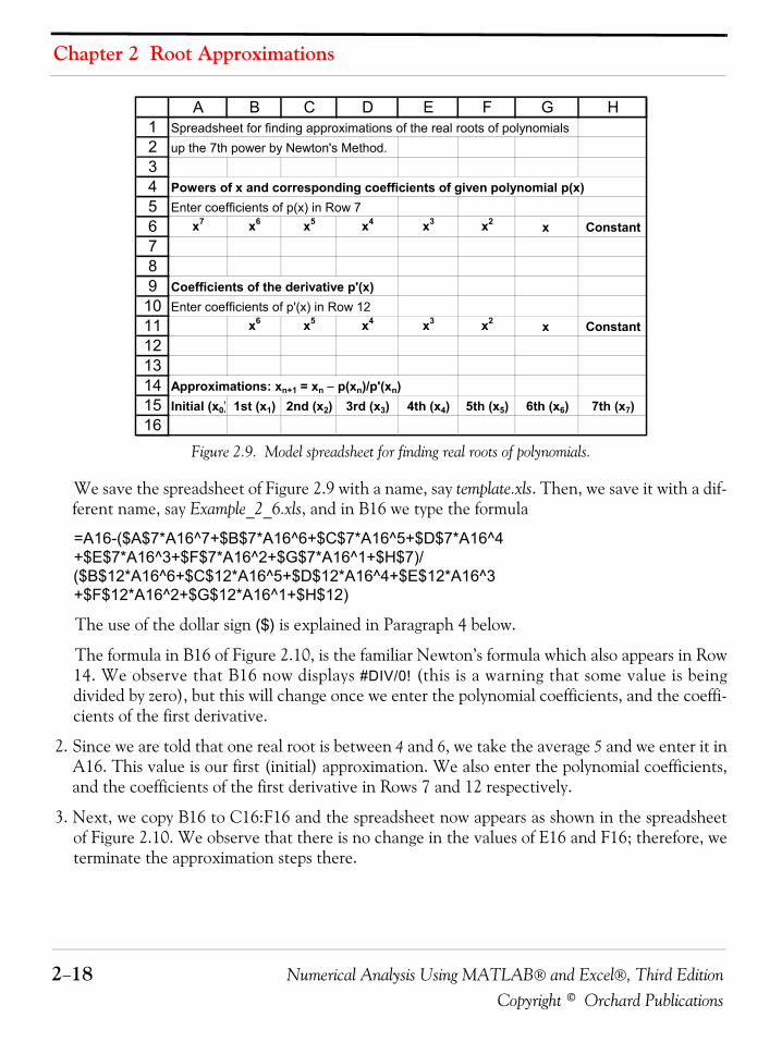
Chapter 2 Root Approximations
2−18 Numerical Analysis Using MATLAB® and Excel®, Third EditionCopyright © Orchard Publications
Figure 2.9. Model spreadsheet for finding real roots of polynomials.
We save the spreadsheet of Figure 2.9 with a name, say template.xls. Then, we save it with a dif-ferent name, say Example_2_6.xls, and in B16 we type the formula
=A16-($A$7*A16^7+$B$7*A16^6+$C$7*A16^5+$D$7*A16^4+$E$7*A16^3+$F$7*A16^2+$G$7*A16^1+$H$7)/($B$12*A16^6+$C$12*A16^5+$D$12*A16^4+$E$12*A16^3+$F$12*A16^2+$G$12*A16^1+$H$12)
The use of the dollar sign ($) is explained in Paragraph 4 below.
The formula in B16 of Figure 2.10, is the familiar Newton’s formula which also appears in Row14. We observe that B16 now displays #DIV/0! (this is a warning that some value is beingdivided by zero), but this will change once we enter the polynomial coefficients, and the coeffi-cients of the first derivative.
2. Since we are told that one real root is between 4 and 6, we take the average 5 and we enter it inA16. This value is our first (initial) approximation. We also enter the polynomial coefficients,and the coefficients of the first derivative in Rows 7 and 12 respectively.
3. Next, we copy B16 to C16:F16 and the spreadsheet now appears as shown in the spreadsheetof Figure 2.10. We observe that there is no change in the values of E16 and F16; therefore, weterminate the approximation steps there.
123456789
10111213141516
A B C D E F G HSpreadsheet for finding approximations of the real roots of polynomials up the 7th power by Newton's Method.
Powers of x and corresponding coefficients of given polynomial p(x) Enter coefficients of p(x) in Row 7
x7 x6 x5 x4 x3 x2 x Constant
Coefficients of the derivative p'(x)Enter coefficients of p'(x) in Row 12
x6 x5 x4 x3 x2 x Constant
Approximations: xn+1 = xn − p(xn)/p'(xn)Initial (x0) 1st (x1) 2nd (x2) 3rd (x3) 4th (x4) 5th (x5) 6th (x6) 7th (x7)
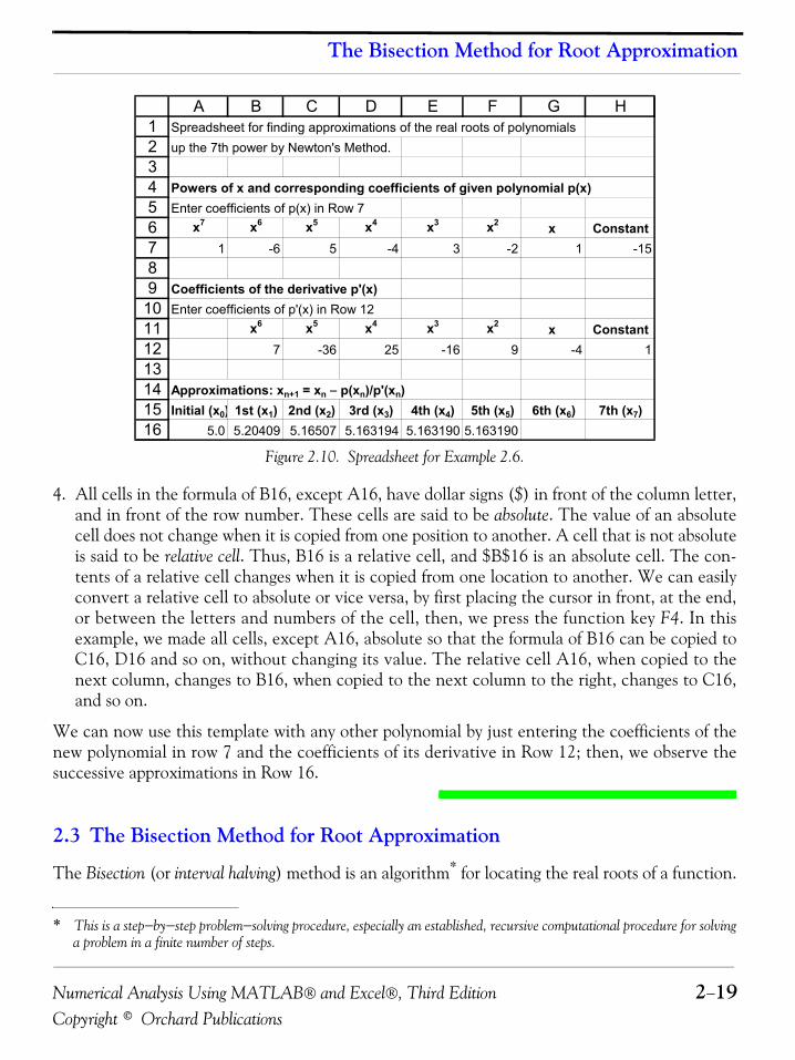
Numerical Analysis Using MATLAB® and Excel®, Third Edition 2−19Copyright © Orchard Publications
The Bisection Method for Root Approximation
Figure 2.10. Spreadsheet for Example 2.6.
4. All cells in the formula of B16, except A16, have dollar signs ($) in front of the column letter,and in front of the row number. These cells are said to be absolute. The value of an absolutecell does not change when it is copied from one position to another. A cell that is not absoluteis said to be relative cell. Thus, B16 is a relative cell, and $B$16 is an absolute cell. The con-tents of a relative cell changes when it is copied from one location to another. We can easilyconvert a relative cell to absolute or vice versa, by first placing the cursor in front, at the end,or between the letters and numbers of the cell, then, we press the function key F4. In thisexample, we made all cells, except A16, absolute so that the formula of B16 can be copied toC16, D16 and so on, without changing its value. The relative cell A16, when copied to thenext column, changes to B16, when copied to the next column to the right, changes to C16,and so on.
We can now use this template with any other polynomial by just entering the coefficients of thenew polynomial in row 7 and the coefficients of its derivative in Row 12; then, we observe thesuccessive approximations in Row 16.
2.3 The Bisection Method for Root Approximation
The Bisection (or interval halving) method is an algorithm* for locating the real roots of a function.
* This is a step−by−step problem−solving procedure, especially an established, recursive computational procedure for solvinga problem in a finite number of steps.
123456789
10111213141516
A B C D E F G HSpreadsheet for finding approximations of the real roots of polynomials up the 7th power by Newton's Method.
Powers of x and corresponding coefficients of given polynomial p(x) Enter coefficients of p(x) in Row 7
x7 x6 x5 x4 x3 x2 x Constant1 -6 5 -4 3 -2 1 -15
Coefficients of the derivative p'(x)Enter coefficients of p'(x) in Row 12
x6 x5 x4 x3 x2 x Constant7 -36 25 -16 9 -4 1
Approximations: xn+1 = xn − p(xn)/p'(xn)Initial (x0) 1st (x1) 2nd (x2) 3rd (x3) 4th (x4) 5th (x5) 6th (x6) 7th (x7)
5.0 5.20409 5.16507 5.163194 5.163190 5.163190
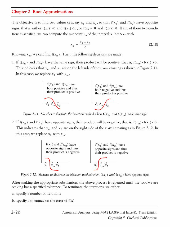
Chapter 2 Root Approximations
2−20 Numerical Analysis Using MATLAB® and Excel®, Third EditionCopyright © Orchard Publications
The objective is to find two values of x, say and , so that and have oppositesigns, that is, either and , or and . If any of these two condi-tions is satisfied, we can compute the midpoint xm of the interval with
(2.18)
Knowing , we can find . Then, the following decisions are made:
1. If and have the same sign, their product will be positive, that is, .This indicates that and are on the left side of the x−axis crossing as shown in Figure 2.11.In this case, we replace with .
Figure 2.11. Sketches to illustrate the bisection method when and have same sign
2. If and have opposite signs, their product will be negative, that is, .This indicates that and are on the right side of the x−axis crossing as in Figure 2.12. Inthis case, we replace with .
Figure 2.12. Sketches to illustrate the bisection method when and have opposite signs
After making the appropriate substitution, the above process is repeated until the root we areseeking has a specified tolerance. To terminate the iterations, we either:
a. specify a number of iterations
b. specify a tolerance on the error of
x1 x2 f x1( ) f x2( )
f x1( ) 0> f x2( ) 0< f x1( ) 0< f x2( ) 0>
x1 x x2≤ ≤
xmx1 x2+
2-----------------=
xm f xm( )
f xm( ) f x1( ) f xm( ) f x1( )⋅ 0>
xm x1
x1 xm
• • •
areboth positive and thus
• • •
their product is positiveboth negative and thus their product is positive
f xm( )f x1( ) and aref xm( )f x1( ) and
x1x1 xmx2xm x2
f x1( ) f xm( )
f xm( ) f x1( ) f xm( ) f x1( )⋅ 0<
xm x2
x2 xm
• • •
opposite signs and thus
• • •
their product is negativeopposite signs and thustheir product is negative
havef xm( )f x1( ) and havef xm( )f x1( ) and
x1 xm x2 x1 xm x2
f x1( ) f xm( )
f x( )
Numerical Analysis Using MATLAB® and Excel®, Third Edition 2−21Copyright © Orchard Publications
The Bisection Method for Root Approximation
We will illustrate the Bisection Method with examples using both MATLAB and Excel.
Example 2.7 Use the Bisection Method with MATLAB to approximate one of the roots of
(2.19)by
a. by specifying 16 iterations, and using a for end loop MATLAB program
b. by specifying 0.00001 tolerance for , and using a while end loop MATLAB program
Solution:
This is the same polynomial as in Example 2.4.
a. The for end loop allows a group of functions to be repeated a fixed and predetermined num-ber of times. The syntax is:
for x = arraycommands...end
Before we write the program script, we must define a function assigned to the given polyno-mial and save it as a function m−file. We will define this function as funcbisect01 and will saveit as funcbisect01.m.
function y= funcbisect01(x);y = 3 .* x .^ 5 − 2 .* x .^ 3 + 6 .* x − 8;% We must not forget to type the semicolon at the end of the line above;% otherwise our script will fill the screen with values of y
On the script below, the statement for k = 1:16 says for , evaluate allcommands down to the end command. After the iteration, the loop ends and anycommands after the end are computed and displayed as commanded.
Let us also review the meaning of the fprintf('%9.6f %13.6f \n', xm,fm) line. Here, %9.6f and%13.6f are referred to as format specifiers or format scripts; the first specifies that the value ofxm must be expressed in decimal format also called fixed point format, with a total of 9 digits, 6of which will be to the right of the decimal point. Likewise, fm must be expressed in decimalformat with a total of 13 digits, 6 of which will be to the right of the decimal point. Some otherspecifiers are %e for scientific format, %s for string format, and %d for integer format. Formore information, we can type help fprintf. The special format \n specifies a linefeed, that is, itprints everything specified up to that point and starts a new line. We will discuss other specialformats as they appear in subsequent examples.
y f x( ) 3x5 2x3– 6x 8–+= =
f x( )
k 1 k, 2 … k, , 16= = =
k 16=
Chapter 2 Root Approximations
2−22 Numerical Analysis Using MATLAB® and Excel®, Third EditionCopyright © Orchard Publications
The script for the first part of Example 2.7 is given below.
x1=1; x2=2; % We know this interval from Example 2.4, Figure 2.6disp(' xm fm') % xm is the average of x1 and x2, fm is f(xm)disp('-------------------------') % insert line under xm and fmfor k=1:16;
f1=funcbisect01(x1); f2=funcbisect01(x2);xm=(x1+x2) / 2; fm=funcbisect01(xm);fprintf('%9.6f %13.6f \n', xm,fm) % Prints xm and fm on same line;if (f1*fm<0) x2=xm;else
x1=xm; end
end
When this program is executed, MATLAB displays the following:
xm fm------------------------- 1.500000 17.031250 1.250000 4.749023 1.125000 1.308441 1.062500 0.038318 1.031250 -0.506944 1.046875 -0.241184 1.054688 -0.103195 1.058594 -0.032885 1.060547 0.002604 1.059570 -0.015168 1.060059 -0.006289 1.060303 -0.001844 1.060425 0.000380 1.060364 -0.000732 1.060394 -0.000176 1.060410 0.000102
We observe that the values are displayed with 6 decimal places as we specified, but for theinteger part unnecessary leading zeros are not displayed.
b. The while end loop evaluates a group of commands an indefinite number of times. The syntaxis:
while expression commands...
Numerical Analysis Using MATLAB® and Excel®, Third Edition 2−23Copyright © Orchard Publications
The Bisection Method for Root Approximation
end
The commands between while and end are executed as long as all elements in expression aretrue. The script should be written so that eventually a false condition is reached and the loopthen terminates.
There is no need to create another function m−file; we will use the same as in part a. Now wetype and execute the following while end loop program.
x1=1; x2=2; tol=0.00001;disp(' xm fm'); disp('-------------------------')while (abs(x1-x2)>2*tol); f1=funcbisect01(x1); f2=funcbisect01(x2); xm=(x1+x2)/2; fm=funcbisect01(xm); fprintf('%9.6f %13.6f \n', xm,fm); if (f1*fm<0); x2=xm; else
x1=xm; endend
When this program is executed, MATLAB displays the following:
xm fm------------------------- 1.500000 17.031250 1.250000 4.749023 1.125000 1.308441 1.062500 0.038318 1.031250 -0.506944 1.046875 -0.241184 1.054688 -0.103195 1.058594 -0.032885 1.060547 0.002604 1.059570 -0.015168 1.060059 -0.006289 1.060303 -0.001844 1.060425 0.000380 1.060364 -0.000732 1.060394 -0.000176 1.060410 0.000102 1.060402 -0.000037 1.060406 0.000032 1.060404 -0.000003
Chapter 2 Root Approximations
2−24 Numerical Analysis Using MATLAB® and Excel®, Third EditionCopyright © Orchard Publications
Next, we will use an Excel spreadsheet to construct a template that approximates a real root of afunction with the bisection method. This requires repeated use of the IF function which has thefollowing syntax.
=IF(logical_test,value_if_true,value_if_false)
where
logical_test: any value or expression that can be evaluated to true or false.
value_if_true: the value that is returned if logical_test is true.
If logical_test is true and value_if_true is omitted, true is returned. Value_if_true can be anotherformula.
value_if_false is the value that is returned if logical_test is false. If logical_test is false andvalue_if_false is omitted, false is returned. Value_if_false can be another formula.
These statements may be clarified with the following examples.
=IF(C11>=1500,A15, B15):If the value in C11 is greater than or equal to 1500, use the value inA15; otherwise use the value in B15.
=IF(D22<E22, 800, 1200):If the value in D22 is less than the value of E22, assign the number800; otherwise assign the number 1200.
=IF(M8<>N17, K7*12, L8/24):If the value in M8 is not equal to the value in N17, use the value inK7 multiplied by 12; otherwise use the value in L8 divided by 24.
Example 2.8
Use the bisection method with an Excel spreadsheet to approximate the value of within0.00001 accuracy.
Solution:
Finding the square root of 5 is equivalent to finding the roots of . We expect the posi-tive root to be in the interval so we assign and . The average of thesevalues is . We will create a template as we did in Example 2.6 so we can use it with anypolynomial equation. We start with a blank spreadsheet and we make the entries in rows 1through 12 as shown in Figure 2.13.
Now, we make the following entries in rows 13 and 14.
A13: 2B13: 3C13: =(A13+B13)/2
5
x2 5– 0=
2 x 3< < x1 2= x2 3=
xm 2.5=
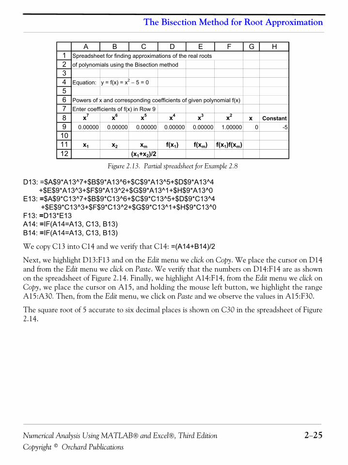
Numerical Analysis Using MATLAB® and Excel®, Third Edition 2−25Copyright © Orchard Publications
The Bisection Method for Root Approximation
Figure 2.13. Partial spreadsheet for Example 2.8
D13: =$A$9*A13^7+$B$9*A13^6+$C$9*A13^5+$D$9*A13^4 +$E$9*A13^3+$F$9*A13^2+$G$9*A13^1+$H$9*A13^0E13: =$A$9*C13^7+$B$9*C13^6+$C$9*C13^5+$D$9*C13^4 +$E$9*C13^3+$F$9*C13^2+$G$9*C13^1+$H$9*C13^0 F13: =D13*E13A14: =IF(A14=A13, C13, B13) B14: =IF(A14=A13, C13, B13)
We copy C13 into C14 and we verify that C14: =(A14+B14)/2
Next, we highlight D13:F13 and on the Edit menu we click on Copy. We place the cursor on D14and from the Edit menu we click on Paste. We verify that the numbers on D14:F14 are as shownon the spreadsheet of Figure 2.14. Finally, we highlight A14:F14, from the Edit menu we click onCopy, we place the cursor on A15, and holding the mouse left button, we highlight the rangeA15:A30. Then, from the Edit menu, we click on Paste and we observe the values in A15:F30.
The square root of 5 accurate to six decimal places is shown on C30 in the spreadsheet of Figure2.14.
123456789
101112
A B C D E F G HSpreadsheet for finding approximations of the real roots of polynomials using the Bisection method
Equation: y = f(x) = x2 − 5 = 0
Powers of x and corresponding coefficients of given polynomial f(x) Enter coefficients of f(x) in Row 9
x7 x6 x5 x4 x3 x2 x Constant0.00000 0.00000 0.00000 0.00000 0.00000 1.00000 0 -5
x1 x2 xm f(x1) f(xm) f(x1)f(xm)(x1+x2)/2
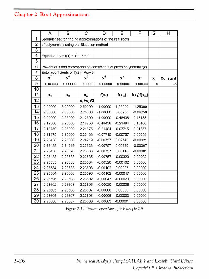
Chapter 2 Root Approximations
2−26 Numerical Analysis Using MATLAB® and Excel®, Third EditionCopyright © Orchard Publications
Figure 2.14. Entire spreadsheet for Example 2.8
123456789
101112131415161718192021222324252627282930
A B C D E F G HSpreadsheet for finding approximations of the real roots of polynomials using the Bisection method
Equation: y = f(x) = x2 − 5 = 0
Powers of x and corresponding coefficients of given polynomial f(x) Enter coefficients of f(x) in Row 9
x7 x6 x5 x4 x3 x2 x Constant0.00000 0.00000 0.00000 0.00000 0.00000 1.00000 0 -5
x1 x2 xm f(x1) f(xm) f(x1)f(xm)(x1+x2)/2
2.00000 3.00000 2.50000 -1.00000 1.25000 -1.250002.00000 2.50000 2.25000 -1.00000 0.06250 -0.062502.00000 2.25000 2.12500 -1.00000 -0.48438 0.484382.12500 2.25000 2.18750 -0.48438 -0.21484 0.104062.18750 2.25000 2.21875 -0.21484 -0.07715 0.016572.21875 2.25000 2.23438 -0.07715 -0.00757 0.000582.23438 2.25000 2.24219 -0.00757 0.02740 -0.000212.23438 2.24219 2.23828 -0.00757 0.00990 -0.000072.23438 2.23828 2.23633 -0.00757 0.00116 -0.000012.23438 2.23633 2.23535 -0.00757 -0.00320 0.000022.23535 2.23633 2.23584 -0.00320 -0.00102 0.000002.23584 2.23633 2.23608 -0.00102 0.00007 0.000002.23584 2.23608 2.23596 -0.00102 -0.00047 0.000002.23596 2.23608 2.23602 -0.00047 -0.00020 0.000002.23602 2.23608 2.23605 -0.00020 -0.00006 0.000002.23605 2.23608 2.23607 -0.00006 0.00000 0.000002.23605 2.23607 2.23606 -0.00006 -0.00003 0.000002.23606 2.23607 2.23606 -0.00003 -0.00001 0.00000
Numerical Analysis Using MATLAB® and Excel®, Third Edition 2−27Copyright © Orchard Publications
Summary
2.4 Summary• Newton’s (or Newton−Raphson) method can be used to approximate the roots of any linear or
non−linear equation of any degree. It uses the formula
To apply Newton’s method, we must begin with a reasonable approximation of the root value.In all cases, this can best be done by plotting versus .
• We can use a spreadsheet to approximate the real roots of linear and non−linear equations butto approximate all roots (real and complex conjugates) it is advisable to use MATLAB.
• The MATLAB the while end loop evaluates a group of statements an indefinite number oftimes and thus can be effectively used for root approximation.
• For approximating real roots we can use Excel’s Goal Seek feature. We use Goal Seek whenwe know the desired result of a single formula, but we do not know the input value which sat-isfies that result. Thus, if we have the function , we can use Goal Seek to set thedependent variable to the desired value (goal) and from it, find the value of the indepen-dent variable which satisfies that goal.
• For repetitive tasks, such as finding the roots of polynomials, it is prudent to construct a tem-plate (model spreadsheet) with the appropriate formulas and then enter the coefficients of thepolynomial to find its real roots.
• The Bisection (or interval halving) method is an algorithm for locating the real roots of afunction. The objective is to find two values of x, say and , so that and haveopposite signs, that is, either and , or and . If any of thesetwo conditions is satisfied, we can compute the midpoint xm of the interval with
• We can use the Bisection Method with MATLAB to approximate one of the roots by specify-ing a number of iterations using a for end or by specifying a tolerance using a while end loop program.
• We can use an Excel spreadsheet to construct a template that approximates a real root of afunction with the bisection method. This requires repeated use of the IF function which hasthe =IF(logical_test,value_if_true,value_if_false)
xn 1+ xnf xn( )f ' xn( )---------------–=
f x( ) x
y f x( )=
yx
x1 x2 f x1( ) f x2( )
f x1( ) 0> f x2( ) 0< f x1( ) 0< f x2( ) 0>
x1 x x2≤ ≤
xmx1 x2+
2-----------------=
Chapter 2 Root Approximations
2−28 Numerical Analysis Using MATLAB® and Excel®, Third EditionCopyright © Orchard Publications
2.5 Exercises
1. Use MATLAB to sketch the graph for each of the following functions, and verifyfrom the graph that and , where and defined below, have opposite signs. Then,use Newton’s method to estimate the root of that lies between and .
a.
b.
Hint: Start with
2. Repeat Exercise 1 above using the Bisection method.
3. Repeat Example 2.5 using MATLAB.
Hint: Use the procedure of Example 2.2
y f x( )=
f a( ) f b( ) a bf x( ) 0= a b
f1 x( ) x4 x 3–+= a 1= b 2=
f2 x( ) 2x 1+ x 4+–= a 2= b 4=
x0 a b+( ) 2⁄=
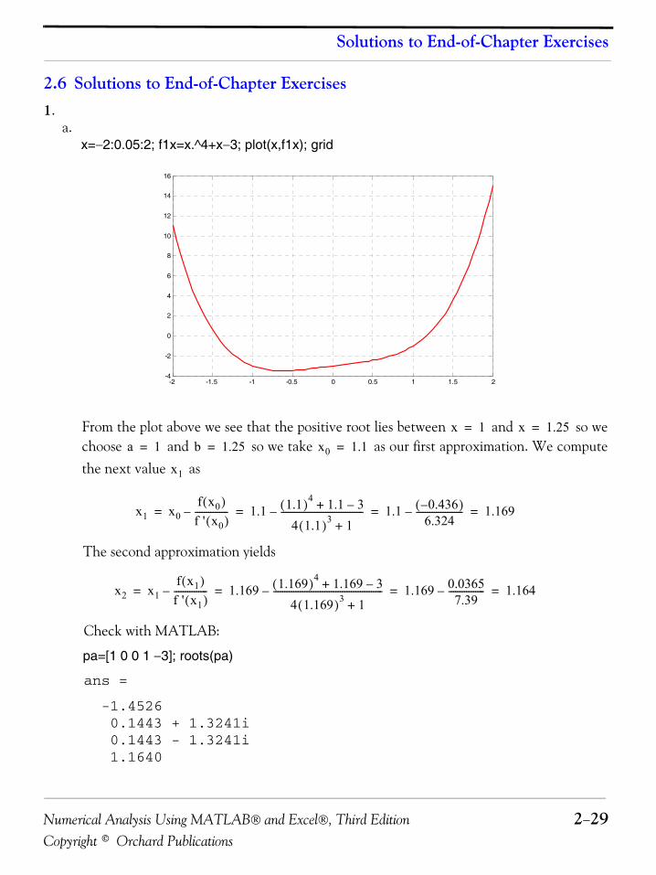
Numerical Analysis Using MATLAB® and Excel®, Third Edition 2−29Copyright © Orchard Publications
Solutions to End-of-Chapter Exercises
2.6 Solutions to End-of-Chapter Exercises1.
a.x=−2:0.05:2; f1x=x.^4+x−3; plot(x,f1x); grid
From the plot above we see that the positive root lies between and so wechoose and so we take as our first approximation. We computethe next value as
The second approximation yields
Check with MATLAB:
pa=[1 0 0 1 −3]; roots(pa)
ans =
-1.4526 0.1443 + 1.3241i 0.1443 - 1.3241i 1.1640
-2 -1.5 -1 -0.5 0 0.5 1 1.5 2-4
-2
0
2
4
6
8
10
12
14
16
x 1= x 1.25=
a 1= b 1.25= x0 1.1=
x1
x1 x0f x0( )f ' x0( )---------------– 1.1 1.1( )4 1.1 3–+
4 1.1( )3 1+-------------------------------------– 1.1 0.436–( )
6.324---------------------– 1.169= = = =
x2 x1f x1( )f ' x1( )---------------– 1.169 1.169( )4 1.169 3–+
4 1.169( )3 1+-------------------------------------------------– 1.169 0.0365
7.39----------------– 1.164= = = =
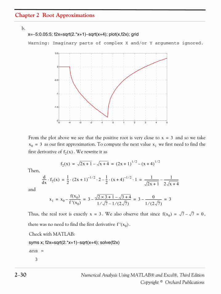
Chapter 2 Root Approximations
2−30 Numerical Analysis Using MATLAB® and Excel®, Third EditionCopyright © Orchard Publications
b.x=−5:0.05:5; f2x=sqrt(2.*x+1)−sqrt(x+4); plot(x,f2x); grid
Warning: Imaginary parts of complex X and/or Y arguments ignored.
From the plot above we see that the positive root is very close to and so we take as our first approximation. To compute the next value we first need to find the
first derivative of . We rewrite it as
Then,
and
Thus, the real root is exactly . We also observe that since ,
there was no need to find the first derivative .
Check with MATLAB:
syms x; f2x=sqrt(2.*x+1)−sqrt(x+4); solve(f2x)
ans =
3
-5 -4 -3 -2 -1 0 1 2 3 4 5-2
-1.5
-1
-0.5
0
0.5
x 3=
x0 3= x1
f2 x( )
f2 x( ) 2x 1+ x 4+– 2x 1+( )1 2⁄ x 4+( )1 2⁄–= =
ddx------ f2 x( )⋅ 1
2--- 2x 1+( ) 1– 2⁄ 2⋅ ⋅ 1
2--- x 4+( ) 1– 2⁄ 1⋅ ⋅– 1
2x 1+------------------- 1
2 x 4+-------------------–= =
x1 x0f x0( )f ' x0( )---------------– 3 2 3 1+× 3 4+–
1 7⁄ 1 2 7( )⁄–------------------------------------------------– 3 0
1 2 7( )⁄----------------------– 3= = = =
x 3= f x0( ) 7 7– 0= =
f ' x0( )
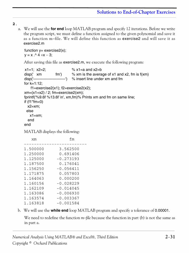
Numerical Analysis Using MATLAB® and Excel®, Third Edition 2−31Copyright © Orchard Publications
Solutions to End-of-Chapter Exercises
2. a. We will use the for end loop MATLAB program and specify 12 iterations. Before we write
the program script, we must define a function assigned to the given polynomial and save itas a function m−file. We will define this function as exercise2 and will save it asexercise2.m
function y= exercise2(x);y = x .^ 4 +x − 3;
After saving this file as exercise2.m, we execute the following program:
x1=1; x2=2; % x1=a and x2=bdisp(' xm fm') % xm is the average of x1 and x2, fm is f(xm)disp('-------------------------') % insert line under xm and fmfor k=1:12;
f1=exercise2(x1); f2=exercise2(x2);xm=(x1+x2) / 2; fm=exercise2(xm);fprintf('%9.6f %13.6f \n', xm,fm)% Prints xm and fm on same line;if (f1*fm<0) x2=xm;else
x1=xm;end
end
MATLAB displays the following:
xm fm-------------------------1.500000 3.562500 1.250000 0.691406 1.125000 -0.273193 1.187500 0.176041 1.156250 -0.056411 1.171875 0.057803
1.164063 0.000200 1.160156 -0.028229 1.162109 -0.014045 1.163086 -0.006930 1.163574 -0.003367 1.163818 -0.001584
b. We will use the while end loop MATLAB program and specify a tolerance of 0.00001.
We need to redefine the function m−file because the function in part (b) is not the same asin part a.
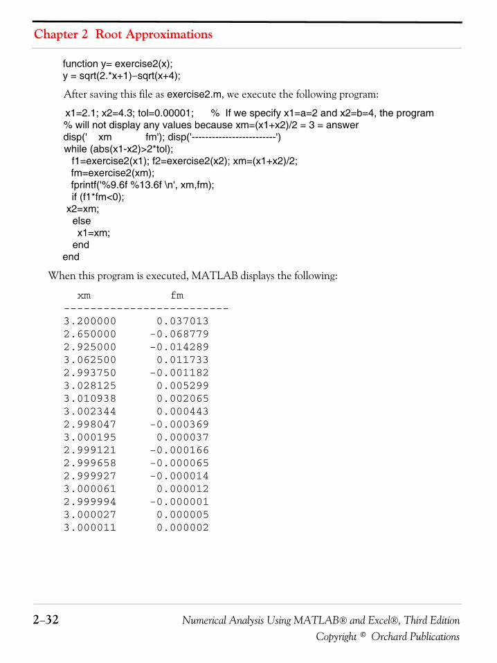
Chapter 2 Root Approximations
2−32 Numerical Analysis Using MATLAB® and Excel®, Third EditionCopyright © Orchard Publications
function y= exercise2(x);y = sqrt(2.*x+1)−sqrt(x+4);
After saving this file as exercise2.m, we execute the following program:
x1=2.1; x2=4.3; tol=0.00001; % If we specify x1=a=2 and x2=b=4, the program% will not display any values because xm=(x1+x2)/2 = 3 = answerdisp(' xm fm'); disp('-------------------------')while (abs(x1-x2)>2*tol); f1=exercise2(x1); f2=exercise2(x2); xm=(x1+x2)/2; fm=exercise2(xm); fprintf('%9.6f %13.6f \n', xm,fm); if (f1*fm<0);
x2=xm; else
x1=xm; endend
When this program is executed, MATLAB displays the following:
xm fm-------------------------
3.200000 0.037013 2.650000 -0.068779 2.925000 -0.014289 3.062500 0.011733 2.993750 -0.001182 3.028125 0.005299 3.010938 0.002065 3.002344 0.000443 2.998047 -0.000369 3.000195 0.000037 2.999121 -0.000166 2.999658 -0.000065 2.999927 -0.000014 3.000061 0.000012 2.999994 -0.000001 3.000027 0.000005 3.000011 0.000002
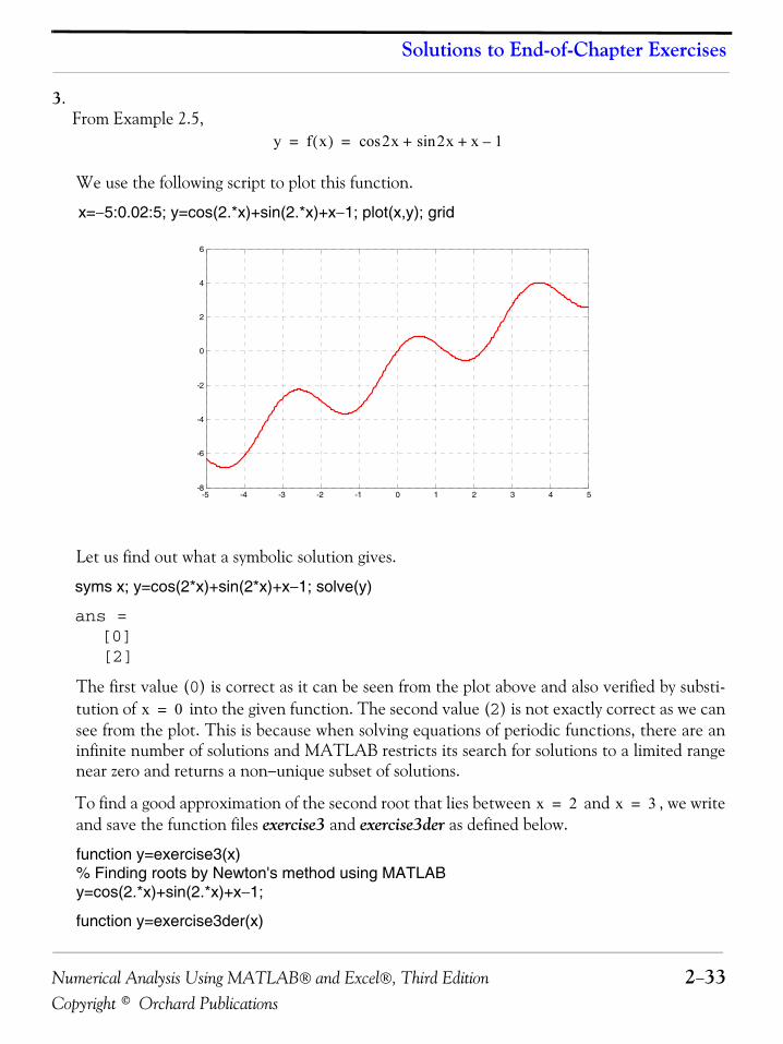
Numerical Analysis Using MATLAB® and Excel®, Third Edition 2−33Copyright © Orchard Publications
Solutions to End-of-Chapter Exercises
3.From Example 2.5,
We use the following script to plot this function.
x=−5:0.02:5; y=cos(2.*x)+sin(2.*x)+x−1; plot(x,y); grid
Let us find out what a symbolic solution gives.
syms x; y=cos(2*x)+sin(2*x)+x−1; solve(y)
ans =[0][2]
The first value (0) is correct as it can be seen from the plot above and also verified by substi-tution of into the given function. The second value (2) is not exactly correct as we cansee from the plot. This is because when solving equations of periodic functions, there are aninfinite number of solutions and MATLAB restricts its search for solutions to a limited rangenear zero and returns a non−unique subset of solutions.
To find a good approximation of the second root that lies between and , we writeand save the function files exercise3 and exercise3der as defined below.
function y=exercise3(x)% Finding roots by Newton's method using MATLABy=cos(2.*x)+sin(2.*x)+x−1;
function y=exercise3der(x)
y f x( ) 2xcos 2x x+sin 1–+= =
-5 -4 -3 -2 -1 0 1 2 3 4 5-8
-6
-4
-2
0
2
4
6
x 0=
x 2= x 3=
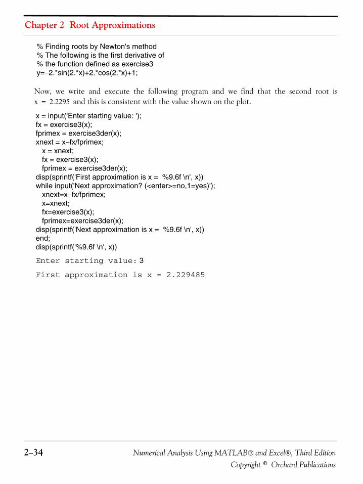
Chapter 2 Root Approximations
2−34 Numerical Analysis Using MATLAB® and Excel®, Third EditionCopyright © Orchard Publications
% Finding roots by Newton's method% The following is the first derivative of% the function defined as exercise3y=−2.*sin(2.*x)+2.*cos(2.*x)+1;
Now, we write and execute the following program and we find that the second root is and this is consistent with the value shown on the plot.
x = input('Enter starting value: ');fx = exercise3(x);fprimex = exercise3der(x);xnext = x−fx/fprimex; x = xnext; fx = exercise3(x); fprimex = exercise3der(x);disp(sprintf('First approximation is x = %9.6f \n', x))while input('Next approximation? (<enter>=no,1=yes)'); xnext=x−fx/fprimex; x=xnext; fx=exercise3(x); fprimex=exercise3der(x);disp(sprintf('Next approximation is x = %9.6f \n', x)) end;disp(sprintf('%9.6f \n', x))
Enter starting value: 3
First approximation is x = 2.229485
x 2.2295=
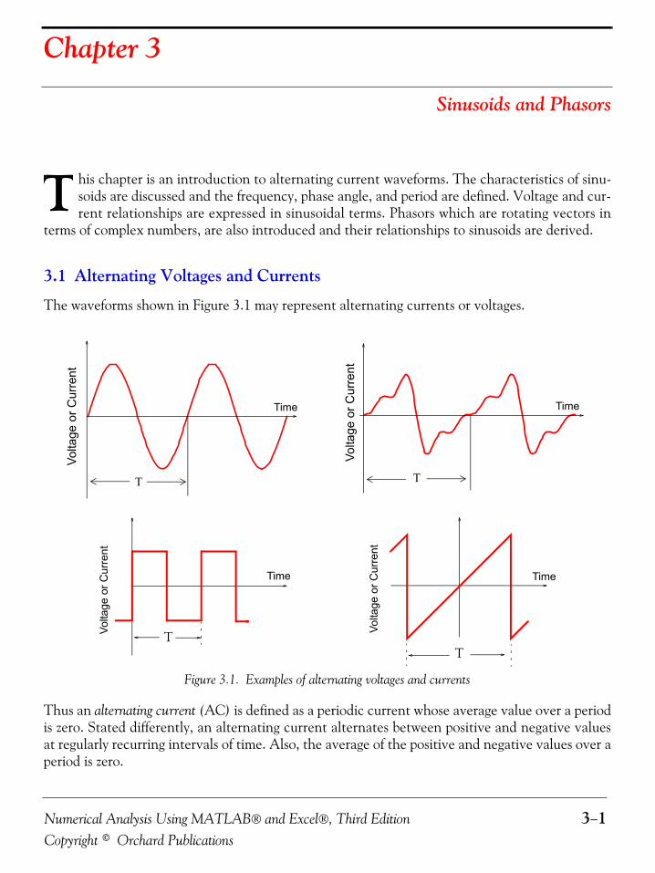
Numerical Analysis Using MATLAB® and Excel®, Third Edition 3−1Copyright © Orchard Publications
Chapter 3
Sinusoids and Phasors
his chapter is an introduction to alternating current waveforms. The characteristics of sinu-soids are discussed and the frequency, phase angle, and period are defined. Voltage and cur-rent relationships are expressed in sinusoidal terms. Phasors which are rotating vectors in
terms of complex numbers, are also introduced and their relationships to sinusoids are derived.
3.1 Alternating Voltages and Currents
The waveforms shown in Figure 3.1 may represent alternating currents or voltages.
Figure 3.1. Examples of alternating voltages and currents
Thus an alternating current (AC) is defined as a periodic current whose average value over a periodis zero. Stated differently, an alternating current alternates between positive and negative valuesat regularly recurring intervals of time. Also, the average of the positive and negative values over aperiod is zero.
T
0 2 4 6 8 10 12-2
-1
0
1
2
0 2 4 6 8 10 12-1
-0.5
0
0.5
1
T T
Volta
ge o
r Cur
rent
Volta
ge o
r Cur
rent
Time Time
T
Time
Volta
ge o
r Cur
rent
Time
T
Volta
ge o
r Cur
rent
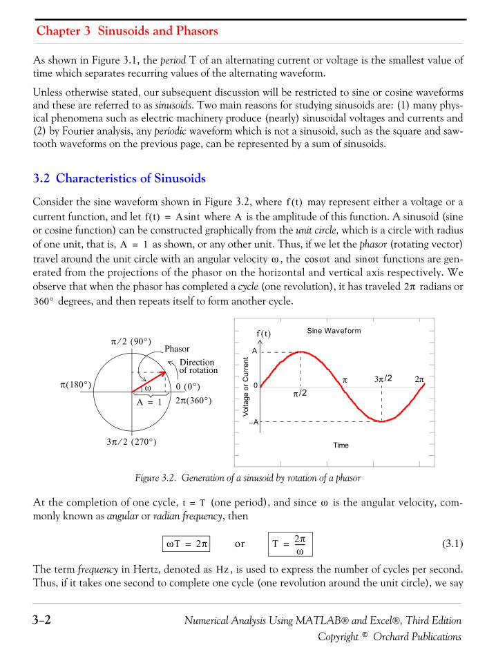
Chapter 3 Sinusoids and Phasors
3−2 Numerical Analysis Using MATLAB® and Excel®, Third EditionCopyright © Orchard Publications
As shown in Figure 3.1, the period T of an alternating current or voltage is the smallest value oftime which separates recurring values of the alternating waveform.
Unless otherwise stated, our subsequent discussion will be restricted to sine or cosine waveformsand these are referred to as sinusoids. Two main reasons for studying sinusoids are: (1) many phys-ical phenomena such as electric machinery produce (nearly) sinusoidal voltages and currents and(2) by Fourier analysis, any periodic waveform which is not a sinusoid, such as the square and saw-tooth waveforms on the previous page, can be represented by a sum of sinusoids.
3.2 Characteristics of Sinusoids
Consider the sine waveform shown in Figure 3.2, where may represent either a voltage or acurrent function, and let where is the amplitude of this function. A sinusoid (sineor cosine function) can be constructed graphically from the unit circle, which is a circle with radiusof one unit, that is, as shown, or any other unit. Thus, if we let the phasor (rotating vector)travel around the unit circle with an angular velocity , the and functions are gen-erated from the projections of the phasor on the horizontal and vertical axis respectively. Weobserve that when the phasor has completed a cycle (one revolution), it has traveled radians or
degrees, and then repeats itself to form another cycle.
Figure 3.2. Generation of a sinusoid by rotation of a phasor
At the completion of one cycle, (one period), and since is the angular velocity, com-monly known as angular or radian frequency, then
(3.1)
The term frequency in Hertz, denoted as , is used to express the number of cycles per second.Thus, if it takes one second to complete one cycle (one revolution around the unit circle), we say
f t( )f t( ) A tsin= A
A 1=
ω ωtcos ωsin t
2π360°
Sine Waveform
Time
Volta
ge o
r Cur
rent
0
A
−A
π /2π 3π /2 2π
Phasor
Directionof rotation
0 0°( )π 180°( )
π 2⁄ 90°( )
3π 2⁄ 270°( )
2π 360°( )A 1=
ω
f t( )
t T= ω
ωT 2π= or T 2πω------=
Hz
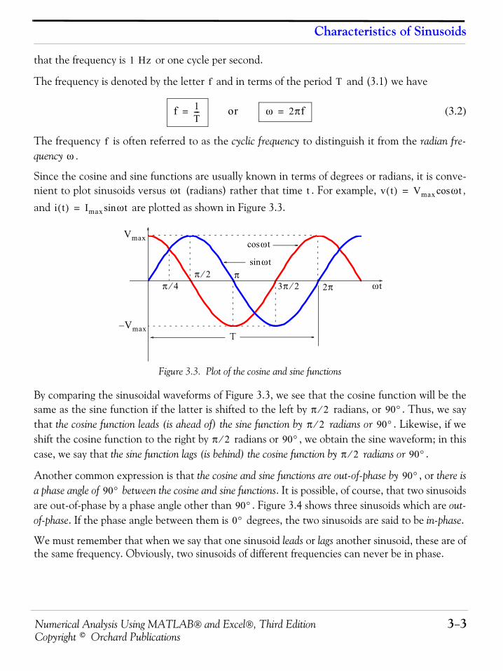
Numerical Analysis Using MATLAB® and Excel®, Third Edition 3−3Copyright © Orchard Publications
Characteristics of Sinusoids
that the frequency is or one cycle per second.
The frequency is denoted by the letter and in terms of the period and (3.1) we have
(3.2)
The frequency is often referred to as the cyclic frequency to distinguish it from the radian fre-quency .
Since the cosine and sine functions are usually known in terms of degrees or radians, it is conve-nient to plot sinusoids versus (radians) rather that time . For example, ,
and are plotted as shown in Figure 3.3.
Figure 3.3. Plot of the cosine and sine functions
By comparing the sinusoidal waveforms of Figure 3.3, we see that the cosine function will be thesame as the sine function if the latter is shifted to the left by radians, or . Thus, we saythat the cosine function leads (is ahead of) the sine function by radians or . Likewise, if weshift the cosine function to the right by radians or , we obtain the sine waveform; in thiscase, we say that the sine function lags (is behind) the cosine function by radians or .
Another common expression is that the cosine and sine functions are out-of-phase by , or there isa phase angle of between the cosine and sine functions. It is possible, of course, that two sinusoidsare out-of-phase by a phase angle other than . Figure 3.4 shows three sinusoids which are out-of-phase. If the phase angle between them is degrees, the two sinusoids are said to be in-phase.
We must remember that when we say that one sinusoid leads or lags another sinusoid, these are ofthe same frequency. Obviously, two sinusoids of different frequencies can never be in phase.
1 Hz
f T
f 1T---= or ω 2πf=
fω
ωt t v t( ) Vmax ωtcos=
i t( ) Imax ωsin t=
0 1 2 3 4 5 6 7-1
-0.5
0
0.5
1
T
ωtsin
ωcos t
ωt2π
Vmax
Vmax–
π 4⁄π 2⁄ π
3π 2⁄
π 2⁄ 90°π 2⁄ 90°
π 2⁄ 90°π 2⁄ 90°
90°90°
90°0°
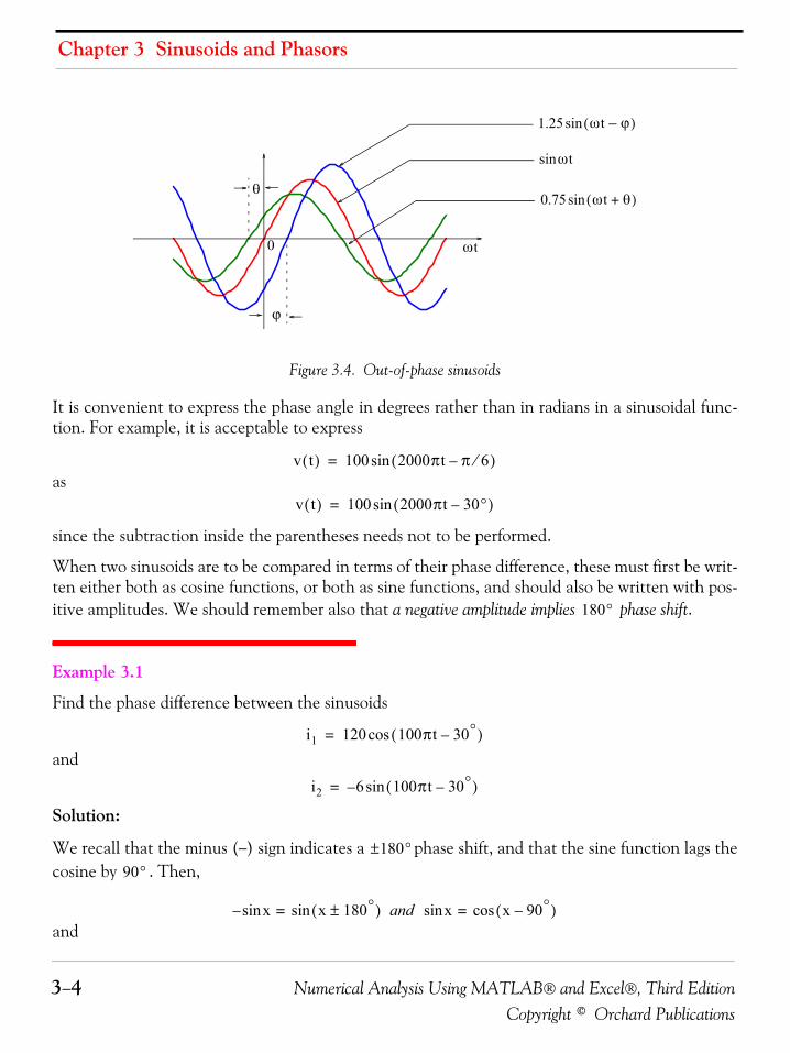
Chapter 3 Sinusoids and Phasors
3−4 Numerical Analysis Using MATLAB® and Excel®, Third EditionCopyright © Orchard Publications
Figure 3.4. Out-of-phase sinusoids
It is convenient to express the phase angle in degrees rather than in radians in a sinusoidal func-tion. For example, it is acceptable to express
as
since the subtraction inside the parentheses needs not to be performed.
When two sinusoids are to be compared in terms of their phase difference, these must first be writ-ten either both as cosine functions, or both as sine functions, and should also be written with pos-itive amplitudes. We should remember also that a negative amplitude implies phase shift.
Example 3.1
Find the phase difference between the sinusoids
and
Solution:
We recall that the minus (−) sign indicates a phase shift, and that the sine function lags thecosine by . Then,
and
-4 -2 0 2 4 6 8-1.5
-1
-0.5
0
0.5
1
1.5
ϕ
θ
ωt0
1.25 ωt ϕ–( )sin
ωtsin
0.75 ωt θ+( )sin
v t( ) 100 2000πt π 6⁄–( )sin=
v t( ) 100 2000πt 30°–( )sin=
180°
i1 120 100πt 30°–( )cos=
i2 6– 100πt 30°–( )sin=
180°±90°
xsin– x 180°±( )sin= and xsin x 90°–( )cos=
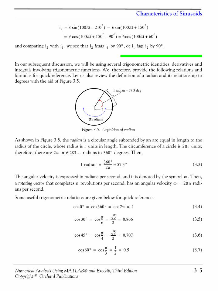
Numerical Analysis Using MATLAB® and Excel®, Third Edition 3−5Copyright © Orchard Publications
Characteristics of Sinusoids
and comparing with , we see that leads by , or lags by .
In our subsequent discussion, we will be using several trigonometric identities, derivatives andintegrals involving trigonometric functions. We, therefore, provide the following relations andformulas for quick reference. Let us also review the definition of a radian and its relationship todegrees with the aid of Figure 3.5.
Figure 3.5. Definition of radian
As shown in Figure 3.5, the radian is a circular angle subtended by an arc equal in length to theradius of the circle, whose radius is units in length. The circumference of a circle is units;therefore, there are or radians in degrees. Then,
(3.3)
The angular velocity is expressed in radians per second, and it is denoted by the symbol . Then,a rotating vector that completes revolutions per second, has an angular velocity radi-ans per second.
Some useful trigonometric relations are given below for quick reference.
(3.4)
(3.5)
(3.6)
(3.7)
i2 6 100πt 210°–( )sin 6 100πt 150°+( )sin= =
6 100πt 150° 90°–+( )cos 6 100πt 60°+( )cos==
i2 i1 i2 i1 90° i1 i2 90°
r
r
π radians
1 radian = 57.3 deg
r 2πr2π 6.283… 360°
1 radian 360°2π
----------- 57.3°≈=
ωn ω 2πn=
0°cos 360°cos 2πcos 1= = =
30°cos π6---cos 3
2------- 0.866= = =
45°cos π4---cos 2
2------- 0.707= = =
60°cos π3---cos 1
2--- 0.5= = =
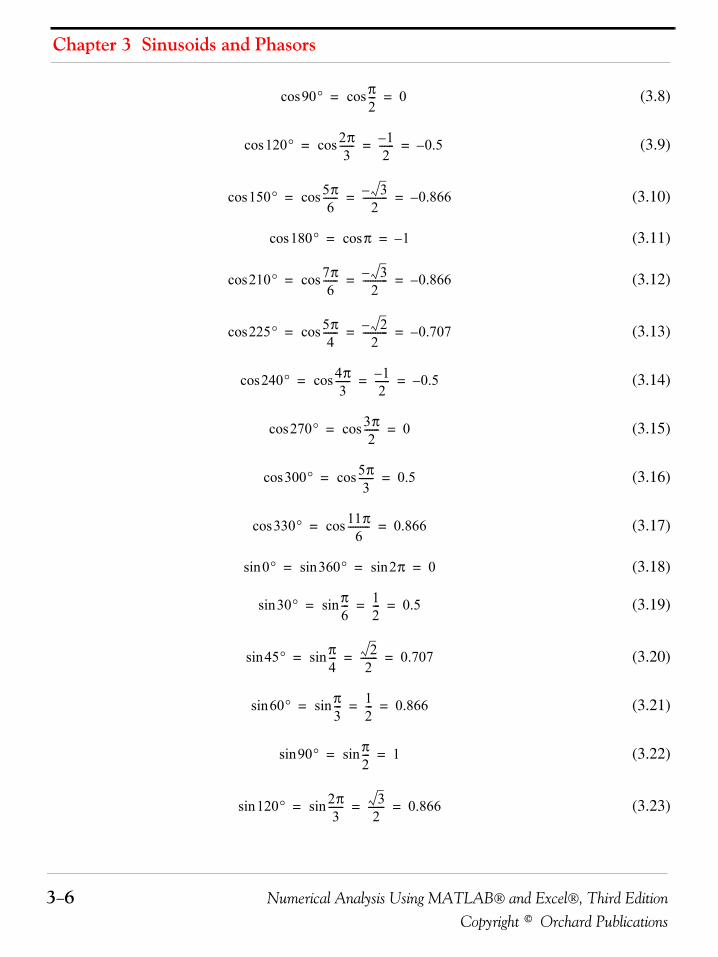
Chapter 3 Sinusoids and Phasors
3−6 Numerical Analysis Using MATLAB® and Excel®, Third EditionCopyright © Orchard Publications
(3.8)
(3.9)
(3.10)
(3.11)
(3.12)
(3.13)
(3.14)
(3.15)
(3.16)
(3.17)
(3.18)
(3.19)
(3.20)
(3.21)
(3.22)
(3.23)
90°cos π2---cos 0= =
120°cos 2π3
------cos 1–2
------ 0.5–= = =
150°cos 5π6
------cos 3–2
---------- 0.866–= = =
180°cos πcos 1–= =
210°cos 7π6
------cos 3–2
---------- 0.866–= = =
225°cos 5π4
------cos 2–2
---------- 0.707–= = =
240°cos 4π3
------cos 1–2
------ 0.5–= = =
270°cos 3π2
------cos 0= =
300°cos 5π3
------cos 0.5= =
330°cos 11π6
---------cos 0.866= =
0sin ° 360sin ° 2sin π 0= = =
30sin ° π6---sin 1
2--- 0.5= = =
45sin ° π4---sin 2
2------- 0.707= = =
60sin ° π3---sin 1
2--- 0.866= = =
90sin ° π2---sin 1= =
120sin ° 2π3
------sin 32
------- 0.866= = =
Numerical Analysis Using MATLAB® and Excel®, Third Edition 3−7Copyright © Orchard Publications
Characteristics of Sinusoids
(3.24)
(3.25)
(3.26)
(3.27)
(3.28)
(3.29)
(3.30)
(3.31)
(3.32)
(3.33)
(3.34)
(3.35)
(3.36)
(3.37)
(3.38)
(3.39)
(3.40)
(3.41)
(3.42)
150sin ° 5π6
------sin 12--- 0.5= = =
180sin ° πsin 0= =
210sin ° 7π6
------sin 1–2
------ 0.5–= = =
225sin ° 5π4
------sin 2–2
---------- 0.707–= = =
240sin ° 4π3
------sin 3–2
---------- 0.866–= = =
270sin ° 3π2
------sin 1–= =
300sin ° 5π3
------sin 3–2
---------- 0.866–= = =
330sin ° 11π6
---------sin 1–2
------ 0.5–= = =
θ–( )cos θcos=
90° θ+( )cos θsin–=
180° θ–( )cos θcos–=
θ–( )sin θsin–=
90° θ+( )sin θcos=
180° θ–( )sin θsin=
θtan θsinθcos
------------=
θcot θcosθsin
------------ 1θtan
-----------= =
θsec 1θcos
------------=
θcsc 1θsin
-----------=
90° θ+( )tan θcot–=
Chapter 3 Sinusoids and Phasors
3−8 Numerical Analysis Using MATLAB® and Excel®, Third EditionCopyright © Orchard Publications
(3.43)
(3.44)
(3.45)
(3.46)
(3.47)
(3.48)
(3.49)
(3.50)
(3.51)
(3.52)
(3.53)
(3.54)
(3.55)
(3.56)
(3.57)
(3.58)
(3.59)
180° θ–( )tan θtan–=
θ φ+( )cos θ φcoscos θsin φsin–=
θ φ–( )cos θ φcoscos θsin φsin+=
θ φ+( )sin θsin φcos θcos φsin+=
θ φ–( )sin θsin φcos θcos– φsin=
θ φ+( )tan θ φtan+tan1 θ φtantan–--------------------------------=
θ φ–( )tan θ φtan–tan1 θ φtantan+--------------------------------=
θ2cos θ2sin+ 1=
2θcos θ2cos θ2sin–=
2sin θ 2 θ θcossin=
2θtan 2 θtan1 θ2tan–----------------------=
θ2cos 12--- 1 2θcos+( )=
θ2sin 12--- 1 2θcos–( )=
θ φcoscos 12--- θ φ+( ) 1
2--- θ φ–( )cos+cos=
θ φsincos 12--- θ φ+( ) 1
2---– θ φ–( )sinsin=
θsin φcos 12--- θ φ+( ) 1
2--- θ φ–( )sin+sin=
θsin φsin 12--- θ φ–( )cos 1
2---– θ φ+( )cos=
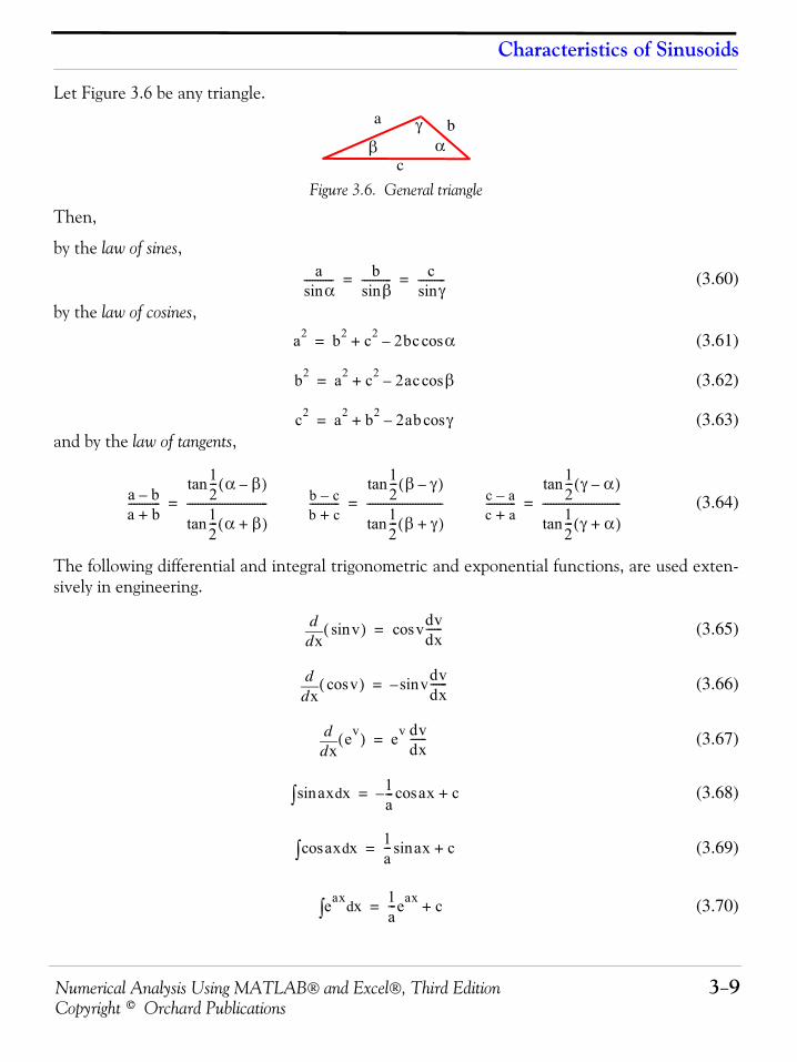
Numerical Analysis Using MATLAB® and Excel®, Third Edition 3−9Copyright © Orchard Publications
Characteristics of Sinusoids
Let Figure 3.6 be any triangle.
Figure 3.6. General triangle
Then,
by the law of sines,
(3.60)
by the law of cosines,
(3.61)
(3.62)
(3.63)and by the law of tangents,
(3.64)
The following differential and integral trigonometric and exponential functions, are used exten-sively in engineering.
(3.65)
(3.66)
(3.67)
(3.68)
(3.69)
(3.70)
β αγa b
c
aαsin
----------- bβsin
----------- cγsin
----------= =
a2 b2 c2 2bc αcos–+=
b2 a2 c2 2ac βcos–+=
c2 a2 b2 2ab γcos–+=
a b–a b+------------
12--- α β–( )tan
12--- α β+( )tan
------------------------------= b c–b c+-----------
12--- β γ–( )tan
12--- β γ+( )tan
----------------------------= c a–c a+-----------
12--- γ α–( )tan
12--- γ α+( )tan
-----------------------------=
xdd vsin( ) vcos dv
dx------=
xdd vcos( ) vsin–
dvdx------=
xdd ev( ) ev dv
dx------=
axsin xd∫1a---– ax c+cos=
acos x xd∫1a--- ax c+sin=
eax xd∫1a---eax c+=
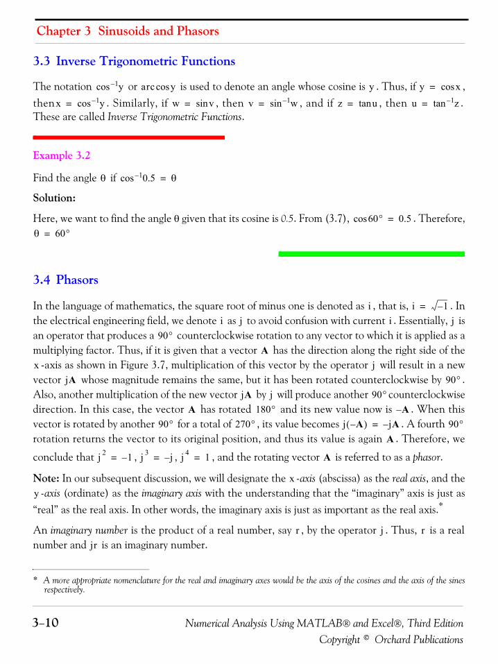
Chapter 3 Sinusoids and Phasors
3−10 Numerical Analysis Using MATLAB® and Excel®, Third EditionCopyright © Orchard Publications
3.3 Inverse Trigonometric Functions
The notation or is used to denote an angle whose cosine is . Thus, if ,then . Similarly, if , then , and if , then .These are called Inverse Trigonometric Functions.
Example 3.2
Find the angle if
Solution:
Here, we want to find the angle θ given that its cosine is 0.5. From (3.7), . Therefore,
3.4 Phasors
In the language of mathematics, the square root of minus one is denoted as , that is, . Inthe electrical engineering field, we denote as to avoid confusion with current . Essentially, isan operator that produces a counterclockwise rotation to any vector to which it is applied as amultiplying factor. Thus, if it is given that a vector has the direction along the right side of the
-axis as shown in Figure 3.7, multiplication of this vector by the operator will result in a newvector whose magnitude remains the same, but it has been rotated counterclockwise by .Also, another multiplication of the new vector by will produce another counterclockwisedirection. In this case, the vector has rotated and its new value now is . When thisvector is rotated by another for a total of , its value becomes . A fourth rotation returns the vector to its original position, and thus its value is again . Therefore, we
conclude that , , , and the rotating vector is referred to as a phasor.
Note: In our subsequent discussion, we will designate the -axis (abscissa) as the real axis, and the-axis (ordinate) as the imaginary axis with the understanding that the “imaginary” axis is just as
“real” as the real axis. In other words, the imaginary axis is just as important as the real axis.*
An imaginary number is the product of a real number, say , by the operator . Thus, is a realnumber and is an imaginary number.
* A more appropriate nomenclature for the real and imaginary axes would be the axis of the cosines and the axis of the sinesrespectively.
y1–cos arc ycos y y xcos=
x y1–cos= w vsin= v w1–sin= z utan= u z1–tan=
θ 0.51–cos θ=
60°cos 0.5=
θ 60°=
i i 1–=
i j i j90°
Ax j
jA 90°jA j 90°
A 180° A–
90° 270° j A–( ) jA–= 90°A
j 2 1–= j 3 j–= j 4 1= A
xy
r j rjr
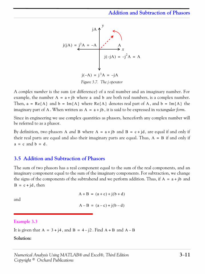
Numerical Analysis Using MATLAB® and Excel®, Third Edition 3−11Copyright © Orchard Publications
Addition and Subtraction of Phasors
Figure 3.7. The j operator
A complex number is the sum (or difference) of a real number and an imaginary number. Forexample, the number where and are both real numbers, is a complex number.Then, and where denotes real part of , and theimaginary part of . When written as , it is said to be expressed in rectangular form.
Since in engineering we use complex quantities as phasors, henceforth any complex number willbe referred to as a phasor.
By definition, two phasors and where and , are equal if and only iftheir real parts are equal and also their imaginary parts are equal. Thus, if and only if
and .
3.5 Addition and Subtraction of Phasors
The sum of two phasors has a real component equal to the sum of the real components, and animaginary component equal to the sum of the imaginary components. For subtraction, we changethe signs of the components of the subtrahend and we perform addition. Thus, if and
, then
and
Example 3.3
It is given that , and . Find and
Solution:
x
yjA
j jA( ) j2A A–= =
j A–( ) j 3A jA–= =
j jA–( ) j– 2A A= =
A
A a jb+= a ba Re A{ }= b Im A{ }= Re A{ } A b Im A{ }=
A A a jb+=
A B A a jb+= B c jd+=
A B=
a c= b d=
A a jb+=
B c jd+=
A B+ a c+( ) j b d+( )+=
A B– a c–( ) j b d–( )+=
A 3 j4+= B 4 j2–= A B+ A B–
Chapter 3 Sinusoids and Phasors
3−12 Numerical Analysis Using MATLAB® and Excel®, Third EditionCopyright © Orchard Publications
3.6 Multiplication of Phasors
Phasors are multiplied using the rules of elementary algebra, and making use of the fact that. Thus, if and , then
and since , it follows that
(3.71)
Example 3.4
It is given that and . Find
Solution:
The conjugate of a phasor, denoted as , is another phasor with the same real component, andwith an imaginary component of opposite sign. Thus, if , then .
Example 3.5
It is given that . Find
Solution:
The conjugate of the phasor has the same real component, but the imaginary component hasopposite sign. Then,
If a phasor is multiplied by its conjugate, the result is a real number. Thus, if , then
A B+ 3 j4+( )= 4 j2–( )+ 3 4+( ) j 4 2–( )+ 7 j2+= =
A B– 3 j4+( )= 4 j2–( )– 3 4–( ) j 4 2+( )+ 1– j6+= =
j 2 1–= A a jb+= B c jd+=
A B⋅ a jb+( ) c jd+( )⋅ ac jad jbc j2bd+ + += =
j 2 1–=
A B⋅ ac jad jbc b– d+ + ac bd–( ) j ad bc+( )+= =
A 3 j4+= B 4 j2–= A B⋅
A B⋅ 3 j4+( ) 4 j2–( )⋅ 12 j6– j16 j 28–+ 20 j10+= = =
A∗
A a jb+= A∗ a j– b=
A 3 j5+= A∗
AA∗ 3 j– 5=
A A a jb+=
A A∗⋅ a jb+( ) a jb–( ) a2 jab– jab j 2b2–+ a2 b2+= = =
Numerical Analysis Using MATLAB® and Excel®, Third Edition 3−13Copyright © Orchard Publications
Division of Phasors
Example 3.6
It is given that . Find
Solution:
3.7 Division of Phasors
When performing division of phasors, it is desirable to obtain the quotient separated into a realpart and an imaginary part. This procedure is called rationalization of the quotient, and it is done bymultiplying the denominator by its conjugate. Thus, if and , then,
(3.72)
In (3.72), we multiplied both the numerator and denominator by the conjugate of the denomina-tor to eliminate the operator from the denominator of the quotient. Using this procedure, wesee that the quotient is easily separated into a real and an imaginary part.
Example 3.7
It is given that , and . Find
Solution:
Using the procedure of (3.72), we get
3.8 Exponential and Polar Forms of Phasors
The relations
(3.73)
and
A 3 j5+= A A∗⋅
A A∗⋅ 3 j5+( ) 3 j5–( ) 32 52+ 9 25 34=+= = =
A a jb+= B c jd+=
AB---- a jb+
c jd+-------------- a jb+( ) c jd–( )
c jd+( ) c jd–( )------------------------------------- A
B---- B∗
B∗-------⋅ ac bd+( ) j bc ad–( )+
c2 d 2+------------------------------------------------------= = = =
ac bd+( )c2 d 2+
----------------------- j bc ad–( )c2 d 2+
----------------------+=
j
A 3 j4+= B 4 j3+= A B⁄
AB---- 3 j4+
4 j3+-------------- 3 j4+( ) 4 j3–( )
4 j3+( ) 4 j3–( )-------------------------------------- 12 j9– j16 12+ +
42 32+-------------------------------------------- 24 j7+
25----------------- 24
25------ j 7
25------+ 0.96 j0.28+= = = = = =
e jθ θ j θsin+cos=
Chapter 3 Sinusoids and Phasors
3−14 Numerical Analysis Using MATLAB® and Excel®, Third EditionCopyright © Orchard Publications
(3.74)
are known as the Euler’s identities.
Multiplying (3.73) by the real positive constant C we get:
(3.75)
This expression represents a phasor, say , and thus
(3.76)
Equating real and imaginary parts in (3.75) and (3.76), we get
(3.77)
Squaring and adding the expressions in (3.77), we get
Then,
or
(3.78)
Also, from (3.77)
or
(3.79)
Therefore, to convert a phasor from rectangular to exponential form, we use the expression
(3.80)
To convert a phasor from exponential to rectangular form, we use the expressions
(3.81)
e jθ– θ j– θsincos=
Ce jθ C θ jC θsin+cos=
a jb+
Ce jθ a jb+=
a C θcos= and b C θsin=
a2 b2+ C θcos( )2 C θsin( )2+ C2 θ2cos θ2sin+( ) C2= = =
C2 a2 b2+=
C a2 b2+=
ba--- C θsin
C θcos--------------- θtan= =
θ ba---⎝ ⎠⎛ ⎞1–tan=
a jb+ a2 b2+ ej tan 1– ba
---⎝ ⎠⎛ ⎞
=
Ce jθ C θ jC θsin+cos=
Ce jθ– C θ j– C θsincos=
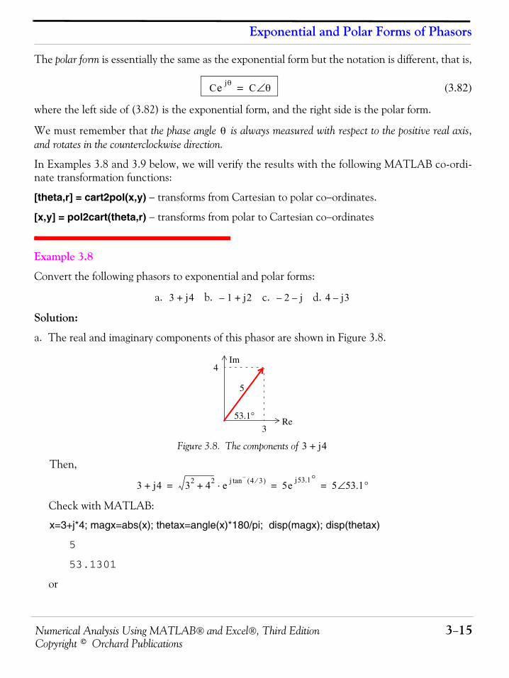
Numerical Analysis Using MATLAB® and Excel®, Third Edition 3−15Copyright © Orchard Publications
Exponential and Polar Forms of Phasors
The polar form is essentially the same as the exponential form but the notation is different, that is,
(3.82)
where the left side of (3.82) is the exponential form, and the right side is the polar form.
We must remember that the phase angle is always measured with respect to the positive real axis,and rotates in the counterclockwise direction.
In Examples 3.8 and 3.9 below, we will verify the results with the following MATLAB co-ordi-nate transformation functions:
[theta,r] = cart2pol(x,y) − transforms from Cartesian to polar co−ordinates.
[x,y] = pol2cart(theta,r) − transforms from polar to Cartesian co−ordinates
Example 3.8
Convert the following phasors to exponential and polar forms:
a. b. c. d.
Solution:
a. The real and imaginary components of this phasor are shown in Figure 3.8.
Figure 3.8. The components of
Then,
Check with MATLAB:
x=3+j*4; magx=abs(x); thetax=angle(x)*180/pi; disp(magx); disp(thetax)
5
53.1301
or
Ce jθ C θ∠=
θ
3 j4+ 1– j2+ 2– j– 4 j3–
Re
Im4
3
5
53.1°
3 j4+
3 j4+ 32 42+ e j 4 3⁄( ) –tan⋅ 5e j53.1° 5 53.1°∠= = =
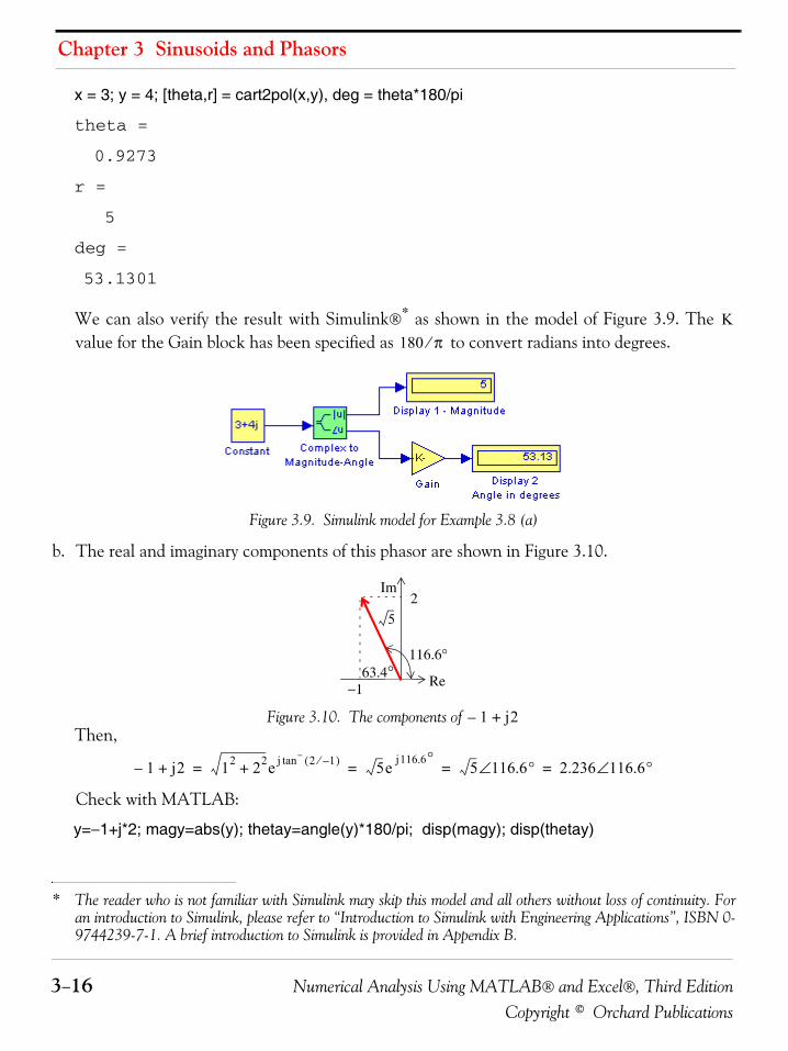
Chapter 3 Sinusoids and Phasors
3−16 Numerical Analysis Using MATLAB® and Excel®, Third EditionCopyright © Orchard Publications
x = 3; y = 4; [theta,r] = cart2pol(x,y), deg = theta*180/pi
theta =
0.9273
r =
5
deg =
53.1301
We can also verify the result with Simulink®* as shown in the model of Figure 3.9. The value for the Gain block has been specified as to convert radians into degrees.
Figure 3.9. Simulink model for Example 3.8 (a)
b. The real and imaginary components of this phasor are shown in Figure 3.10.
Figure 3.10. The components of Then,
Check with MATLAB:
y=−1+j*2; magy=abs(y); thetay=angle(y)*180/pi; disp(magy); disp(thetay)
* The reader who is not familiar with Simulink may skip this model and all others without loss of continuity. Foran introduction to Simulink, please refer to “Introduction to Simulink with Engineering Applications”, ISBN 0-9744239-7-1. A brief introduction to Simulink is provided in Appendix B.
K180 π⁄
Re
Im2
−1
116.6°63.4°
5
1– j2+
1– j2+ 12 22+ e j 2 1–⁄( ) –tan 5e j116.6° 5 116.6°∠ 2.236 116.6°∠= = = =
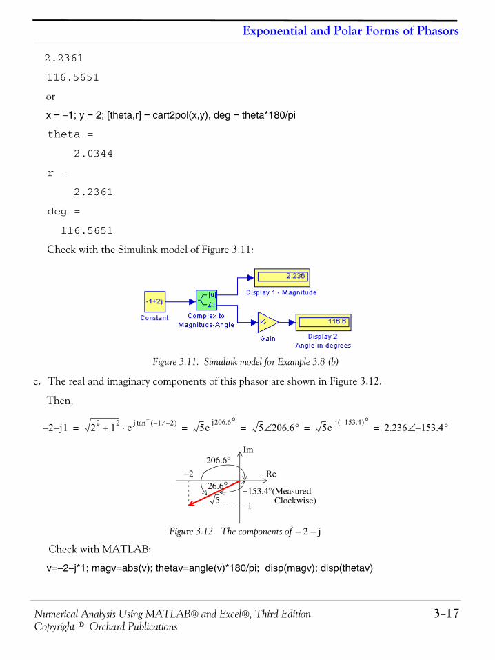
Numerical Analysis Using MATLAB® and Excel®, Third Edition 3−17Copyright © Orchard Publications
Exponential and Polar Forms of Phasors
2.2361
116.5651
or
x = −1; y = 2; [theta,r] = cart2pol(x,y), deg = theta*180/pi
theta =
2.0344
r =
2.2361
deg =
116.5651
Check with the Simulink model of Figure 3.11:
Figure 3.11. Simulink model for Example 3.8 (b)
c. The real and imaginary components of this phasor are shown in Figure 3.12.
Then,
Figure 3.12. The components of
Check with MATLAB:
v=−2−j*1; magv=abs(v); thetav=angle(v)*180/pi; disp(magv); disp(thetav)
2– j– 1 22 12+ e j 1– 2–⁄( ) –tan⋅ 5e j206.6° 5 206.6°∠ 5e j 153.4–( )° 2.236 153.4– °∠= = = = =
Re
Im
−2
−1
206.6°
−153.4°(Measured26.6°Clockwise)5
2– j–
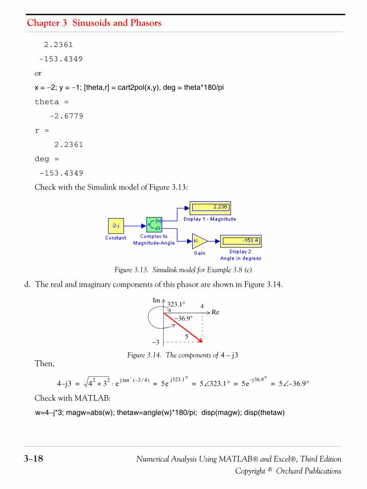
Chapter 3 Sinusoids and Phasors
3−18 Numerical Analysis Using MATLAB® and Excel®, Third EditionCopyright © Orchard Publications
2.2361
-153.4349
or
x = −2; y = −1; [theta,r] = cart2pol(x,y), deg = theta*180/pi
theta =
-2.6779
r =
2.2361
deg =
-153.4349
Check with the Simulink model of Figure 3.13:
Figure 3.13. Simulink model for Example 3.8 (c)
d. The real and imaginary components of this phasor are shown in Figure 3.14.
Figure 3.14. The components of Then,
Check with MATLAB:
w=4−j*3; magw=abs(w); thetaw=angle(w)*180/pi; disp(magw); disp(thetaw)
Re
Im4
−35
323.1°
−36.9°
4 j3–
4 j– 3 42 32+ e j 3– 4⁄( ) –tan⋅ 5e j323.1° 5 323.1°∠ 5e j36.9– ° 5 36.9– °∠= = = = =
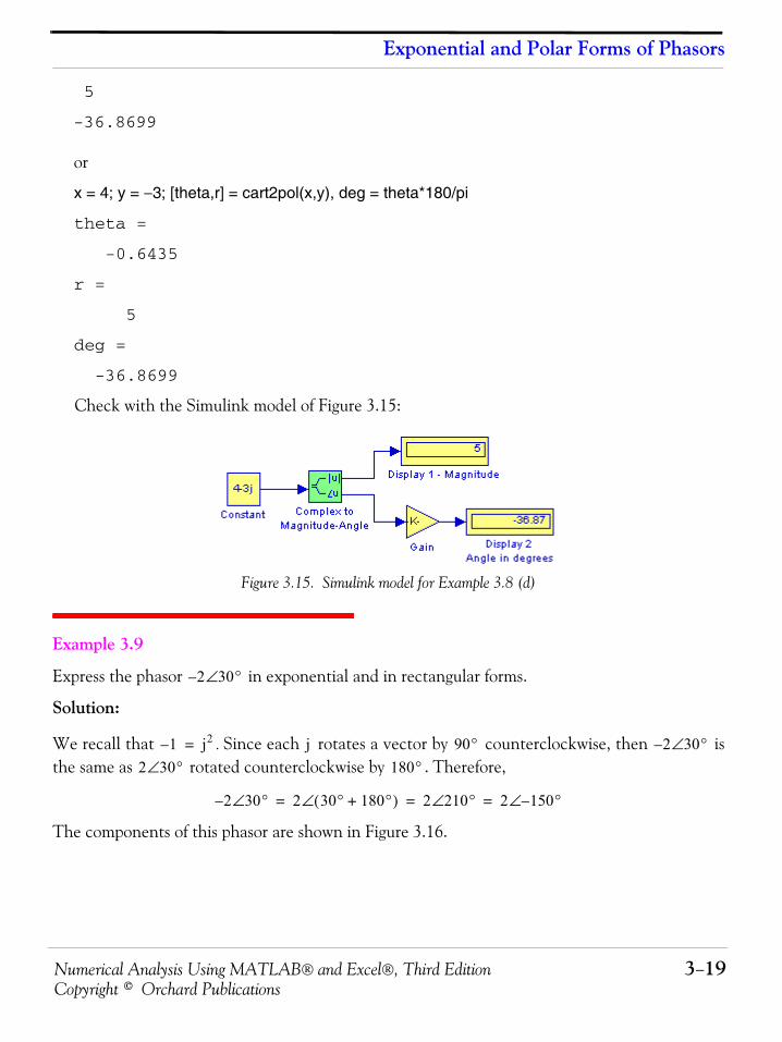
Numerical Analysis Using MATLAB® and Excel®, Third Edition 3−19Copyright © Orchard Publications
Exponential and Polar Forms of Phasors
5
-36.8699
or
x = 4; y = −3; [theta,r] = cart2pol(x,y), deg = theta*180/pi
theta =
-0.6435
r =
5
deg =
-36.8699
Check with the Simulink model of Figure 3.15:
Figure 3.15. Simulink model for Example 3.8 (d)
Example 3.9
Express the phasor in exponential and in rectangular forms.
Solution:
We recall that . Since each rotates a vector by counterclockwise, then isthe same as rotated counterclockwise by . Therefore,
The components of this phasor are shown in Figure 3.16.
2 30°∠–
1– j2= j 90° 2 30°∠–
2 30°∠ 180°
2 30°∠– 2 30° 180°+( )∠ 2 210°∠ 2 150°–∠= = =
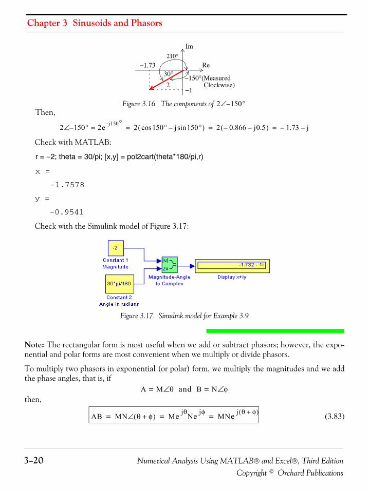
Chapter 3 Sinusoids and Phasors
3−20 Numerical Analysis Using MATLAB® and Excel®, Third EditionCopyright © Orchard Publications
Figure 3.16. The components of Then,
Check with MATLAB:
r = −2; theta = 30/pi; [x,y] = pol2cart(theta*180/pi,r)
x =
-1.7578
y =
-0.9541
Check with the Simulink model of Figure 3.17:
Figure 3.17. Simulink model for Example 3.9
Note: The rectangular form is most useful when we add or subtract phasors; however, the expo-nential and polar forms are most convenient when we multiply or divide phasors.
To multiply two phasors in exponential (or polar) form, we multiply the magnitudes and we addthe phase angles, that is, if
then,
(3.83)
Re
Im
−1.73
−1
210°
2−150°(Measured
30°Clockwise)
2 150°–∠
2 150– °∠ 2e j– 150°= 2 150° j 150°sin–cos( ) 2 0.866– j0.5–( ) 1.73– j–= = =
A M θ∠= and B N φ∠=
AB MN θ φ+( )∠ Me jθNe jφ MNe j θ φ+( )= = =
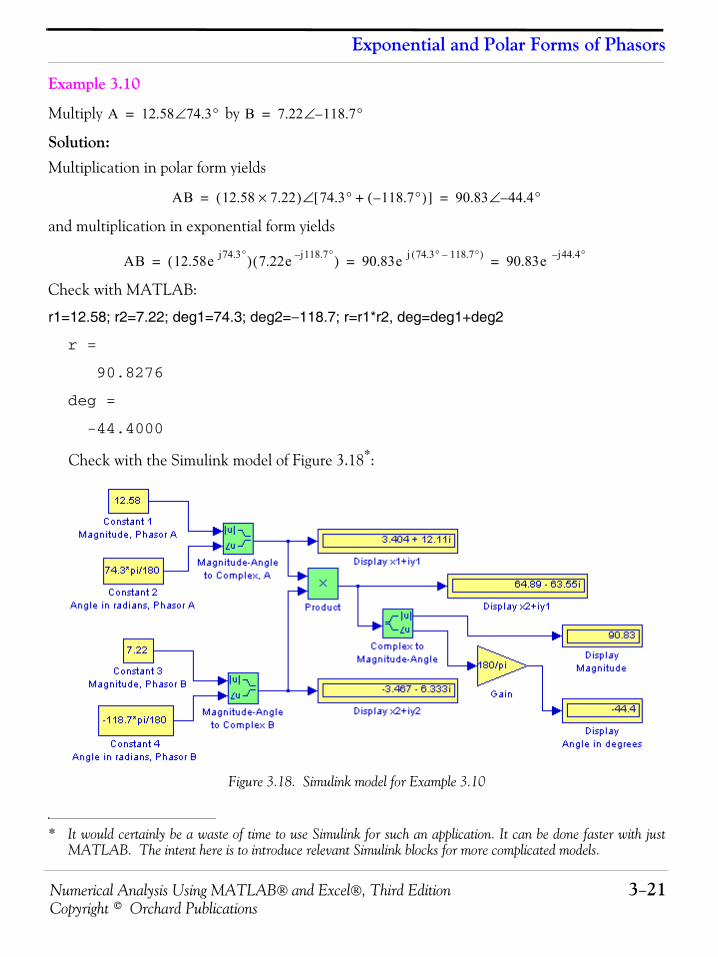
Numerical Analysis Using MATLAB® and Excel®, Third Edition 3−21Copyright © Orchard Publications
Exponential and Polar Forms of Phasors
Example 3.10
Multiply by
Solution:Multiplication in polar form yields
and multiplication in exponential form yields
Check with MATLAB:
r1=12.58; r2=7.22; deg1=74.3; deg2=−118.7; r=r1*r2, deg=deg1+deg2
r =
90.8276
deg =
-44.4000
Check with the Simulink model of Figure 3.18*:
Figure 3.18. Simulink model for Example 3.10
* It would certainly be a waste of time to use Simulink for such an application. It can be done faster with justMATLAB. The intent here is to introduce relevant Simulink blocks for more complicated models.
A 12.58 74.3°∠= B 7.22 118.7°–∠=
AB 12.58 7.22×( ) 74.3° 118.7°–( )+[ ]∠ 90.83 44.4– °∠= =
AB 12.58e j74.3°( ) 7.22e j– 118.7°( ) 90.83e j 74.3° 118.7°–( ) 90.83e j– 44.4°= = =
Chapter 3 Sinusoids and Phasors
3−22 Numerical Analysis Using MATLAB® and Excel®, Third EditionCopyright © Orchard Publications
To divide one phasor by another when both are expressed in exponential or polar form, we dividethe magnitude of the dividend by the magnitude of the divisor, and we subtract the phase angle ofthe divisor from the phase angle of the dividend, that is, if
then,
(3.84)
Example 3.11
Divide by
Solution:
Division in polar form yields
Division in exponential form yields
Check with MATLAB:
r1=12.58; r2=7.22; deg1=74.3; deg2=−118.7; r=r1/r2, deg=deg1−deg2
r =
1.7424
deg =
193
Check with the Simulink model of Figure 3.19*:
* Same comment as on the footnote of the previous page.
A M θ∠= and B N φ∠=
AB---- M
N----- θ φ–( )∠ Me jθ
Ne jφ------------- M
N----e j θ φ–( )
= = =
A 12.58 74.3°∠= B 7.22 118.7°–∠=
AB---- 12.58 74.3°∠
7.22 118.7°–∠---------------------------------- 1.74 74.3° 118.7°–( )–[ ]∠ 1.74 193°∠ 1.74 167– °∠= = = =
AB---- 12.58e j74.3°
7.22e j118.7°–----------------------------- 1.74e j74.3°e j118.7° 1.74e j193° 1.74e j– 167°= = = =
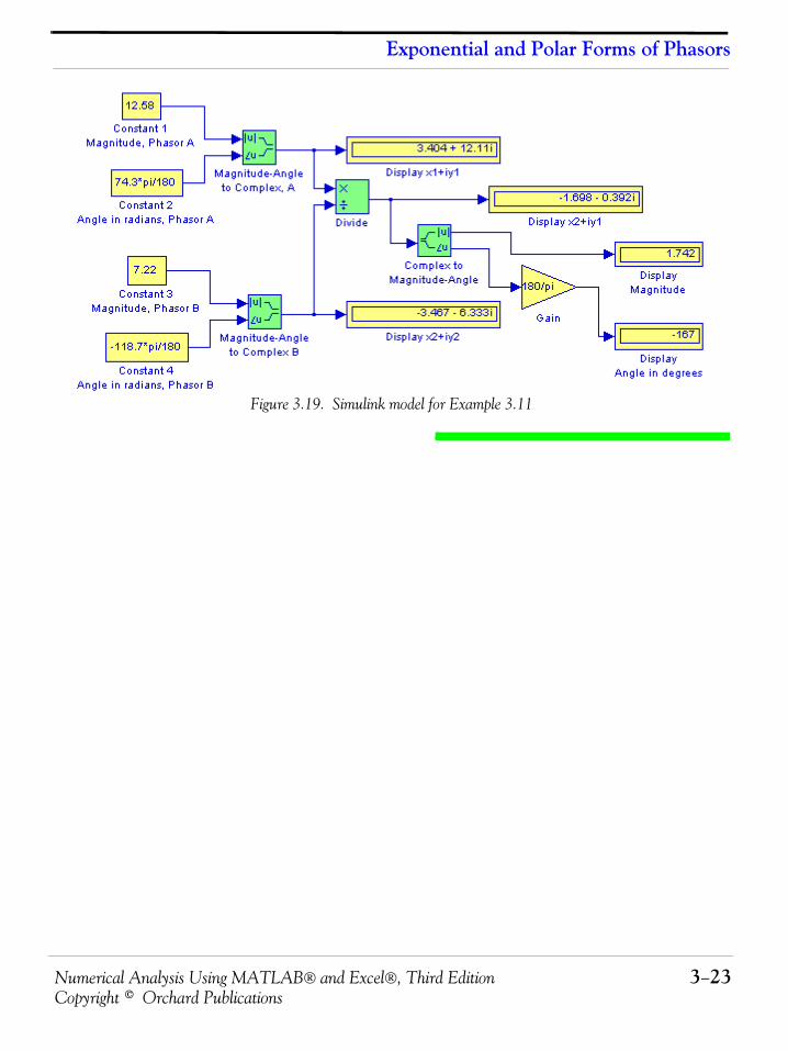
Numerical Analysis Using MATLAB® and Excel®, Third Edition 3−23Copyright © Orchard Publications
Exponential and Polar Forms of Phasors
Figure 3.19. Simulink model for Example 3.11
Chapter 3 Sinusoids and Phasors
3−24 Numerical Analysis Using MATLAB® and Excel®, Third EditionCopyright © Orchard Publications
3.9 Summary
• An alternating current (or voltage) alternates between positive and negative values at regularlyrecurring intervals of time.
• The period T of an alternating current or voltage is the smallest value of time which separatesrecurring values of the alternating waveform.
• Sine and cosine waveforms and these are referred to as sinusoids.
• The angular velocity is commonly known as angular or radian frequency and
• The term frequency in Hertz, denoted as , is used to express the number of cycles per sec-ond. The frequency is denoted by the letter and in terms of the period , . The fre-quency is often referred to as the cyclic frequency to distinguish it from the radian frequency
.
• The cosine function leads (is ahead of) the sine function by radians or , and the sinefunction lags (is behind) the cosine function by radians or . Alternately, we say thatthe cosine and sine functions are out-of-phase by , or there is a phase angle of betweenthe cosine and sine functions.
• Two (or more) sinusoids can be out-of-phase by a phase angle other than .
• It is important to remember that when we say that one sinusoid leads or lags another sinusoid,these are of the same frequency since two sinusoids of different frequencies can never be inphase.
• It is customary to express the phase angle in degrees rather than in radians in a sinusoidal func-tion. For example, we write as
• When two sinusoids are to be compared in terms of their phase difference, these must first bewritten either both as cosine functions, or both as sine functions, and should also be writtenwith positive amplitudes.
• A negative amplitude implies phase shift.
• The radian is a circular angle subtended by an arc equal in length to the radius of the circle,whose radius is units in length. The circumference of a circle is .
• The notation or is used to denote an angle whose cosine is . Thus, if, then . These are called Inverse Trigonometric Functions.
• A phasor is a rotating vector expressed as a complex number where is an operator thatrotates a vector by in a counterclockwise direction.
ω ωT 2π=
Hzf T f 1 T⁄=
fω
π 2⁄ 90°π 2⁄ 90°90° 90°
90°
v t( ) 100 2000πt π 6⁄–( )sin= v t( ) 100 2000πt 30°–( )sin=
180°
r 2πr
y1–cos arc ycos yy xcos= x y1–cos=
j90°
Numerical Analysis Using MATLAB® and Excel®, Third Edition 3−25Copyright © Orchard Publications
Summary
• Two phasors and where and , are equal if and only if their realparts are equal and also their imaginary parts are equal. Thus, if and only if and
.
• The sum of two phasors has a real component equal to the sum of the real components, and animaginary component equal to the sum of the imaginary components. For subtraction, wechange the signs of the components of the subtrahend and we perform addition. Thus, if
and , then and
• Phasors are multiplied using the rules of elementary algebra. If and ,then
• The conjugate of a phasor, denoted as , is another phasor with the same real component,and with an imaginary component of opposite sign. Thus, if , then .
• When performing division of phasors, it is desirable to obtain the quotient separated into areal part and an imaginary part. This is achieved by multiplying the denominator by its conju-gate. Thus, if and , then,
• The relations and are known as the Euler’s identi-ties.
• To convert a phasor from rectangular to exponential form, we use the expression
• To convert a phasor from exponential to rectangular form, we use the expressions
• The polar form is essentially the same as the exponential form but the notation is different,that is,
and it is important to remember that the phase angle is always measured with respect to thepositive real axis, and rotates in the counterclockwise direction.
• The rectangular form is most useful when we add or subtract phasors; however, the exponen-tial and polar forms are most convenient when we multiply or divide phasors.
A B A a jb+= B c jd+=
A B= a c=
b d=
A a jb+= B c jd+= A B+ a c+( ) j b d+( )+= A B– a c–( ) j b d–( )+=
A a jb+= B c jd+=
A B⋅ ac jad jbc b– d+ + ac bd–( ) j ad bc+( )+= =
A∗
A a jb+= A∗ a j– b=
A a jb+= B c jd+=
AB---- a jb+
c jd+-------------- a jb+( ) c jd–( )
c jd+( ) c jd–( )------------------------------------- ac bd+( ) j bc ad–( )+
c2 d 2+------------------------------------------------------ ac bd+( )
c2 d 2+----------------------- j bc ad–( )
c2 d 2+----------------------+= = = =
e jθ θ j θsin+cos= e jθ– θ j– θsincos=
a jb+ a2 b2+ ej tan 1– b
a---⎝ ⎠
⎛ ⎞=
Ce jθ C θ jC θsin+cos=
Ce jθ– C θ j– C θsincos=
Ce jθ C θ∠=
θ
Chapter 3 Sinusoids and Phasors
3−26 Numerical Analysis Using MATLAB® and Excel®, Third EditionCopyright © Orchard Publications
• To multiply two phasors in exponential (or polar) form, we multiply the magnitudes and weadd the phase angles, that is, if
then,
• To divide one phasor by another when both are expressed in exponential or polar form, wedivide the magnitude of the dividend by the magnitude of the divisor, and we subtract thephase angle of the divisor from the phase angle of the dividend, that is, if
then,
A M θ∠= and B N φ∠=
AB MN θ φ+( )∠ Me jθNe jφ MNe j θ φ+( )= = =
A M θ∠= and B N φ∠=
AB---- M
N----- θ φ–( )∠ Me jθ
Ne jφ------------- M
N----e j θ φ–( )
= = =
Numerical Analysis Using MATLAB® and Excel®, Third Edition 3−27Copyright © Orchard Publications
Exercises
3.10 Exercises
1. Perform the following operations, and check your answers with MATLAB.
a. b. c. d.
e. f. g.
2. Perform the following operations, and check your answers with MATLAB.
a. b. c. d.
3. Any phasor can be expressed as
Using the identities or , compute:
a. b.
Check your answers with MATLAB
4. Compute the exponential and polar forms of
a. b.
Check your answers with MATLAB.
5. Compute the rectangular form of
a. b.
Check your answers with MATLAB
6. Find the real and imaginary components of
2 j4–( ) 3 j4+( )+ 3– j5+( ) 1 j6+( )– 2 j3–( ) 2 j3–( )∗– 3 j2–( ) 3 j2–( )∗⋅
2 j4–( ) 3 j5+( )⋅ 3 j2–( ) 2– j3–( )⋅ 2 j4–( ) 3 j5+( ) 3 j2–( ) 2– j3–( )⋅ ⋅ ⋅
22 j6+3 j2+
----------------- 8 j6+3– j–
--------------- 1204 j10–----------------- 3 j2–( )
3 j2–( )∗---------------------
A
A a jb+ r θ j θsin+cos( ) re jθ= = =
re jθ( ) rne jnθ= re jθn rn e jθ n⁄=
12 j5+6 100 2 1 j–( )4
9 j5+4– j2–
------------------ 8– j3+2– j4+
------------------
4 30°∠5 150°–∠---------------------- e j60°
2e j30°––-------------------
9 j4–5– jx+
------------------
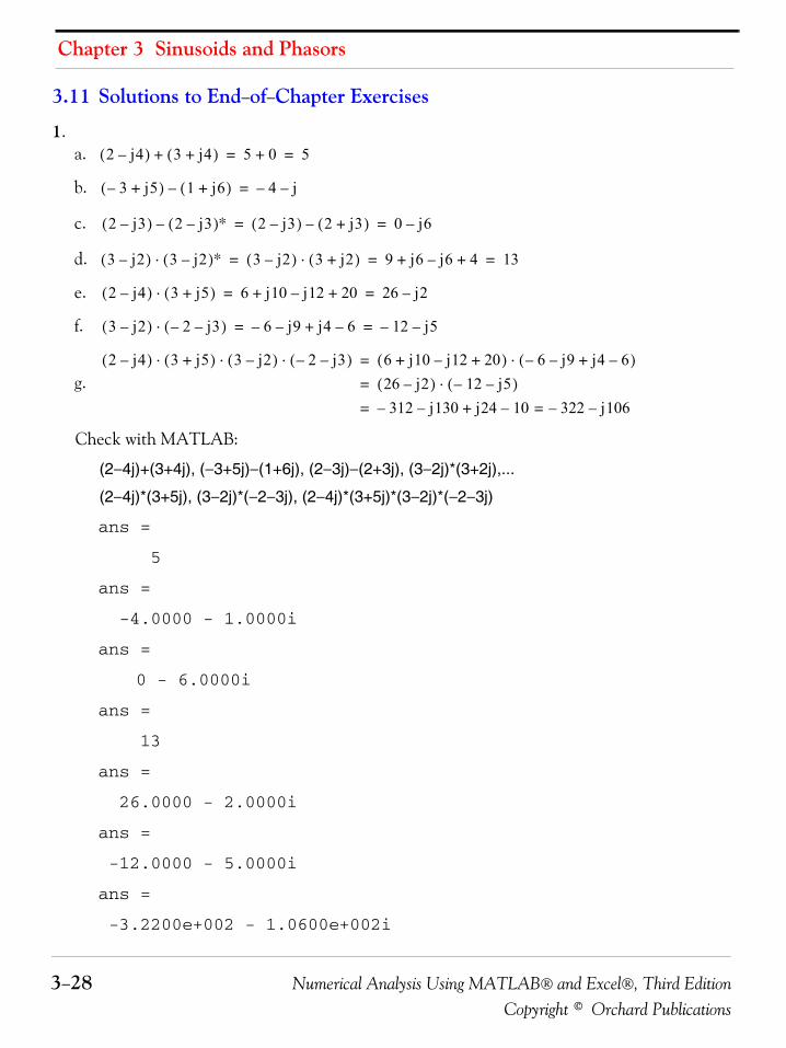
Chapter 3 Sinusoids and Phasors
3−28 Numerical Analysis Using MATLAB® and Excel®, Third EditionCopyright © Orchard Publications
3.11 Solutions to End−of−Chapter Exercises
1.a.
b.
c.
d.
e.
f.
g.
Check with MATLAB:
(2−4j)+(3+4j), (−3+5j)−(1+6j), (2−3j)−(2+3j), (3−2j)*(3+2j),...
(2−4j)*(3+5j), (3−2j)*(−2−3j), (2−4j)*(3+5j)*(3−2j)*(−2−3j)
ans =
5
ans =
-4.0000 - 1.0000i
ans =
0 - 6.0000i
ans =
13
ans =
26.0000 - 2.0000i
ans =
-12.0000 - 5.0000i
ans =
-3.2200e+002 - 1.0600e+002i
2 j4–( ) 3 j4+( )+ 5 0+ 5= =
3– j5+( ) 1 j6+( )– 4– j–=
2 j3–( ) 2 j3–( )∗– 2 j3–( ) 2 j3+( )– 0 j6–= =
3 j2–( ) 3 j2–( )∗⋅ 3 j2–( ) 3 j2+( )⋅ 9 j6 j6– 4+ + 13= = =
2 j4–( ) 3 j5+( )⋅ 6 j10 j12– 20+ + 26 j2–= =
3 j2–( ) 2– j3–( )⋅ 6– j9– j4 6–+ 12– j5–= =
2 j4–( ) 3 j5+( ) 3 j2–( ) 2– j3–( )⋅ ⋅ ⋅ 6 j10 j12– 20+ +( ) 6– j9– j4 6–+( )⋅=
26 j2–( ) 12– j5–( )⋅=
312– j130– j24 10–+ 322– j106–==
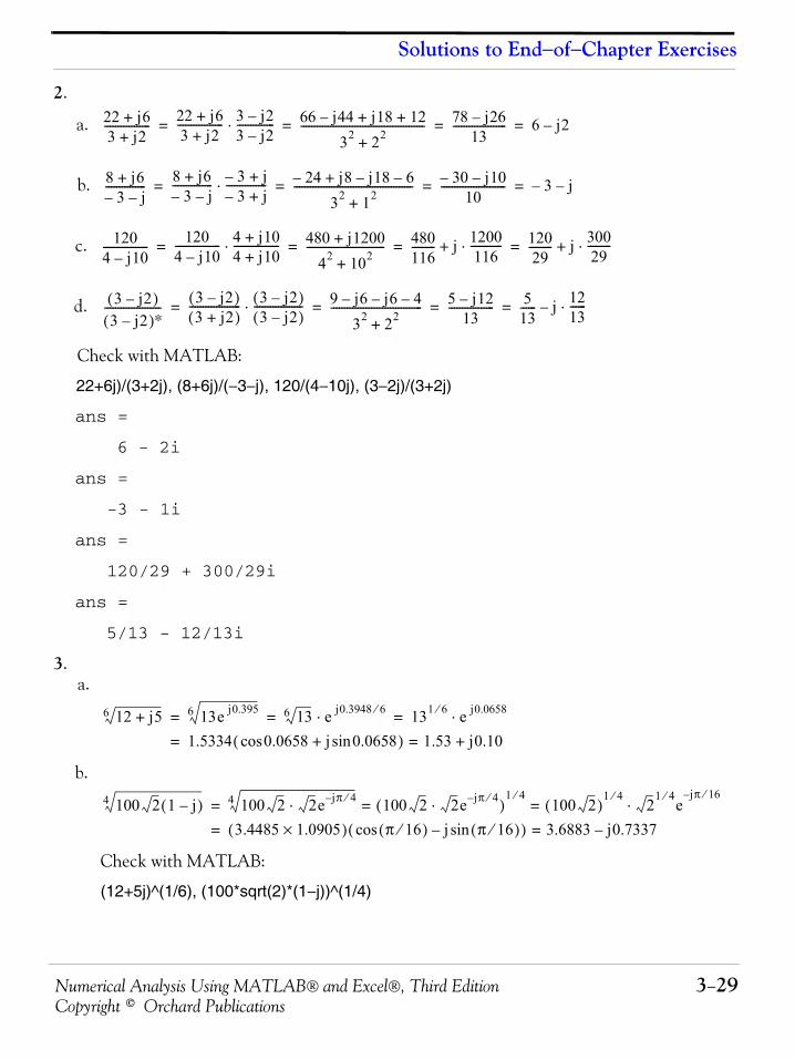
Numerical Analysis Using MATLAB® and Excel®, Third Edition 3−29Copyright © Orchard Publications
Solutions to End−of−Chapter Exercises
2.
a.
b.
c.
d.
Check with MATLAB:
22+6j)/(3+2j), (8+6j)/(−3−j), 120/(4−10j), (3−2j)/(3+2j)
ans =
6 - 2i
ans =
-3 - 1i
ans =
120/29 + 300/29i
ans =
5/13 - 12/13i
3.a.
b.
Check with MATLAB:
(12+5j)^(1/6), (100*sqrt(2)*(1−j))^(1/4)
22 j6+3 j2+
----------------- 22 j6+3 j2+
----------------- 3 j2–3 j2–--------------⋅ 66 j44– j18 12+ +
32 22+---------------------------------------------- 78 j26–
13-------------------- 6 j2–= = = =
8 j6+3– j–
--------------- 8 j6+3– j–
--------------- 3– j+3– j+
---------------⋅ 24– j8 j18– 6–+
32 12+-------------------------------------------- 30– j10–
10------------------------ 3– j–= = = =
1204 j10–----------------- 120
4 j10–----------------- 4 j10+
4 j10+-----------------⋅ 480 j1200+
42 102+----------------------------- 480
116--------- j 1200
116------------⋅+ 120
29--------- j 300
29---------⋅+= = = =
3 j2–( )3 j2–( )∗
--------------------- 3 j2–( )3 j2+( )
------------------- 3 j2–( )3 j2–( )
------------------⋅ 9 j6– j6– 4–
32 22+---------------------------------- 5 j12–
13----------------- 5
13------ j 12
13------⋅–= = = =
12 j5+6 13e j0.3956 136 e j0.3948 6⁄⋅ 131 6⁄ e j0.0658⋅= = =
1.5334 0.0658 j 0.0658sin+cos( ) 1.53 j0.10+==
100 2 1 j–( )4 100 2 2e jπ 4⁄–⋅4 100 2 2e jπ 4⁄–⋅( )1 4⁄
100 2( )1 4⁄
21 4⁄
ejπ– 16⁄
⋅= ==
3.4485 1.0905×( ) π 16⁄( ) j π 16⁄( )sin–cos( ) 3.6883 j0.7337–==
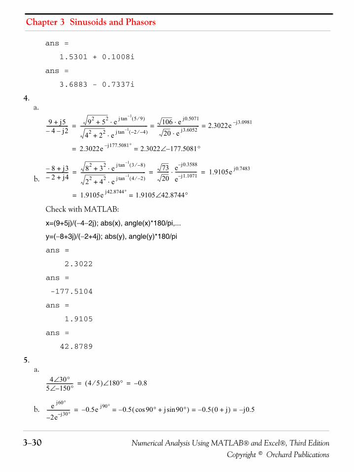
Chapter 3 Sinusoids and Phasors
3−30 Numerical Analysis Using MATLAB® and Excel®, Third EditionCopyright © Orchard Publications
ans =
1.5301 + 0.1008i
ans =
3.6883 - 0.7337i
4.a.
b.
Check with MATLAB:
x=(9+5j)/(−4−2j); abs(x), angle(x)*180/pi,...
y=(−8+3j)/(−2+4j); abs(y), angle(y)*180/pi
ans =
2.3022
ans =
-177.5104
ans =
1.9105
ans =
42.8789
5.a.
b.
9 j5+4– j2–
------------------ 92 52+ e j 5 9⁄( )1–tan⋅
42 22+ e j 2– 4–⁄( )1–tan⋅-------------------------------------------------------- 106 e j0.5071⋅
20 e j3.6052⋅----------------------------------- 2.3022e j– 3.0981= ==
2.3022e j177.5081– ° 2.3022 177.5081– °∠==
8– j3+2– j4+
------------------ 82 32+ e j 3 8–⁄( )1–tan⋅
22 42+ e j 4 2–⁄( )1–tan⋅------------------------------------------------------ 73
20---------- e j0.3588–
e j1.1071–------------------⋅ 1.9105e j0.7483= = =
1.9105e j42.8744° 1.9105 42.8744°∠==
4 30°∠5 150°–∠---------------------- 4 5⁄( ) 180°∠ 0.8–= =
e j60°
2e j30°––------------------- 0.5e j90° 0.5 90° j 90°sin+cos( )– 0.5 0 j+( )– j0.5–= = =–=
Numerical Analysis Using MATLAB® and Excel®, Third Edition 3−31Copyright © Orchard Publications
Solutions to End−of−Chapter Exercises
Check with MATLAB:
4*(cos(pi/6)+sin(pi/6)*j)/(5*(cos(−5*pi/6)+sin(−5*pi/6)*j)),...
exp(pi*j/3)/(−2*exp(−pi*j/6))
ans =
-0.8000 - 0.0000i
ans =
-0.0000 - 0.5000i
6.
9 j4–5– jx+
------------------ 9 j4–5– jx+
------------------ 5– j– x5– j– x
--------------⋅ 45– j9x– j20 4x–+
52 x2+--------------------------------------------------- 4x– 45–
x2 25+---------------------- j 9x– 20+
x2 25+-----------------------+= = =
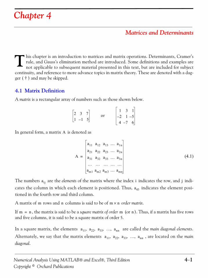
Numerical Analysis Using MATLAB® and Excel®, Third Edition 4−1Copyright © Orchard Publications
Chapter 4
Matrices and Determinants
his chapter is an introduction to matrices and matrix operations. Determinants, Cramer’srule, and Gauss’s elimination method are introduced. Some definitions and examples arenot applicable to subsequent material presented in this text, but are included for subject
continuity, and reference to more advance topics in matrix theory. These are denoted with a dag-ger ( † ) and may be skipped.
4.1 Matrix DefinitionA matrix is a rectangular array of numbers such as those shown below.
In general form, a matrix is denoted as
(4.1)
The numbers are the elements of the matrix where the index indicates the row, and indi-cates the column in which each element is positioned. Thus, indicates the element posi-tioned in the fourth row and third column.
A matrix of rows and columns is said to be of order matrix.
If , the matrix is said to be a square matrix of order (or ). Thus, if a matrix has five rowsand five columns, it is said to be a square matrix of order 5.
In a square matrix, the elements are called the main diagonal elements.
Alternately, we say that the matrix elements , are located on the main
diagonal.
T
2 3 71 1– 5
or1 3 12– 1 5–4 7– 6
A
A
a11 a12 a13 … a1n
a21 a22 a23 … a2n
a31 a32 a33 … a3n
… … … … …am1 am2 am3 … amn
=
aij i j
a43
m n m n×
m n= m n
a11 a22 a33 … ann, , , ,
a11 a22 a33 … ann, , , ,
Chapter 4 Matrices and Determinants
4−2 Numerical Analysis Using MATLAB® and Excel®, Third EditionCopyright © Orchard Publications
† The sum of the diagonal elements of a square matrix is called the trace* of .
† A matrix in which every element is zero, is called a zero matrix.
4.2 Matrix Operations
Two matrices and are equal, that is, , if and only if
(4.2)
Two matrices are said to be conformable for addition (subtraction), if they are of the same order.
If and are conformable for addition (subtraction), their sum (difference) will
be another matrix with the same order as and , where each element of is the sum (dif-ference) of the corresponding elements of and , that is,
(4.3)
Example 4.1
Compute and given that
and
Solution:
and
Check with MATLAB:
A=[1 2 3; 0 1 4]; B=[2 3 0; −1 2 5]; % Define matrices A and BA+B % Add A and B
* Henceforth, all paragraphs and topics preceded by a dagger ( † ) may be skipped. These are discussed in matrix theory text-books.
A A
A aij= B bij= A B=
aij bij= i 1 2 3 … m, , , ,= j 1 2 3 … n, , , ,=
m n×
A aij= B bij=
C A B CA B
C A B± aij bij±[ ]= =
A B+ A B–
A 1 2 30 1 4
= B 2 3 01– 2 5
=
A B+ 1 2+ 2 3+ 3 0+0 1– 1 2+ 4 5+
3 5 31– 3 9
= =
A B– 1 2– 2 3– 3 0–0 1+ 1 2– 4 5–
1– 1– 31 1– 1–
= =
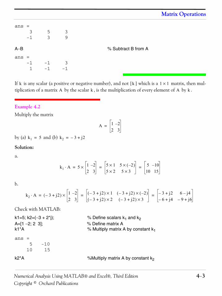
Numerical Analysis Using MATLAB® and Excel®, Third Edition 4−3Copyright © Orchard Publications
Matrix Operations
ans = 3 5 3 -1 3 9
A−B % Subtract B from A
ans = -1 -1 3 1 -1 -1
If is any scalar (a positive or negative number), and not [ ] which is a matrix, then mul-tiplication of a matrix by the scalar , is the multiplication of every element of by .
Example 4.2 Multiply the matrix
by (a) and (b)
Solution:
a.
b.
Check with MATLAB:
k1=5; k2=(−3 + 2*j); % Define scalars k1 and k2A=[1 −2; 2 3]; % Define matrix Ak1*A % Multiply matrix A by constant k1
ans = 5 -10 10 15
k2*A %Multiply matrix A by constant k2
k k 1 1×A k A k
A 1 2–2 3
=
k1 5= k2 3– j2+=
k1 A⋅ 5 1 2–2 3
× 5 1× 5 2–( )×5 2× 5 3×
5 10–10 15
= = =
k2 A⋅ 3– j2+( ) 1 2–2 3
× 3– j2+( ) 1× 3– j2+( ) 2–( )×3– j2+( ) 2× 3– j2+( ) 3×
3– j2+ 6 j4–6– j4+ 9– j6+
= = =
Chapter 4 Matrices and Determinants
4−4 Numerical Analysis Using MATLAB® and Excel®, Third EditionCopyright © Orchard Publications
ans = -3.0000+ 2.0000i 6.0000- 4.0000i -6.0000+ 4.0000i -9.0000+ 6.0000i
Two matrices and are said to be conformable for multiplication in that order, only whenthe number of columns of matrix is equal to the number of rows of matrix . That is, the prod-uct (but not ) is conformable for multiplication only if is an and matrix isan matrix. The product will then be an matrix. A convenient way to determineif two matrices are conformable for multiplication is to write the dimensions of the two matricesside−by−side as shown below.
For the product we have:
For matrix multiplication, the operation is row by column. Thus, to obtain the product , wemultiply each element of a row of by the corresponding element of a column of ; then, weadd these products.
Example 4.3 Given that
and
compute the products and
Solution:
The dimensions of matrices and are respectively ; therefore the product is
A B A B⋅A B
A B⋅ B A⋅ A m p× Bp n× A B⋅ m n×
m × p p × nA B
Shows that A and B are conformable for multiplication
Indicates the dimension of the product A ⋅ B
B A⋅
Here, B and A are not conformable for multiplication
B A p × n m × p
A B⋅A B
C 2 3 4= D11–2
=
C D⋅ D C⋅
C D 1 3 3 1×× C D⋅
Numerical Analysis Using MATLAB® and Excel®, Third Edition 4−5Copyright © Orchard Publications
Special Forms of Matrices
feasible, and will result in a , that is,
The dimensions for and are respectively and therefore, the product is alsofeasible. Multiplication of these will produce a 3 × 3 matrix as follows.
Check with MATLAB:
C=[2 3 4]; D=[1; −1; 2]; % Define matrices C and DC*D % Multiply C by D
ans = 7
D*C % Multiply D by C
ans = 2 3 4 -2 -3 -4 4 6 8
Division of one matrix by another, is not defined. However, an equivalent operation exists, and itwill become apparent later in this chapter, when we discuss the inverse of a matrix.
4.3 Special Forms of Matrices† A square matrix is said to be upper triangular when all the elements below the diagonal are
zero. The matrix below is an upper triangular matrix.
(4.4)
1 1×
C D⋅ 2 3 411–2
2( ) 1( )⋅ 3( ) 1–( )⋅ 4( ) 2( )⋅+ + 7= = =
D C 3 1 1 3×× D C⋅
D C⋅11–2
2 3 41( ) 2( )⋅ 1( ) 3( )⋅ 1( ) 4( )⋅1–( ) 2( )⋅ 1–( ) 3( )⋅ 1–( ) 4( )⋅
2( ) 2( )⋅ 2( ) 3( )⋅ 2( ) 4( )⋅
2 3 42– 3– 4–4 6 8
= = =
A
A
a11 a12 a13 … a1n
0 a22 a23 … a2n
0 0 … … …… … 0 … …0 0 0 … amn
=
Chapter 4 Matrices and Determinants
4−6 Numerical Analysis Using MATLAB® and Excel®, Third EditionCopyright © Orchard Publications
In an upper triangular matrix, not all elements above the diagonal need to be non−zero. Forapplications, refer to Chapter 14.
† A square matrix is said to be lower triangular, when all the elements above the diagonal arezero. The matrix below is a lower triangular matrix. For applications, refer to Chapter 14.
(4.5)
In a lower triangular matrix, not all elements below the diagonal need to be non−zero.
† A square matrix is said to be diagonal, if all elements are zero, except those in the diagonal. Thematrix below is a diagonal matrix.
(4.6)
† A diagonal matrix is called a scalar matrix, if where is a sca-lar. The matrix below is a scalar matrix with .
(4.7)
A scalar matrix with , is called an identity matrix . Shown below are , , and identity matrices.
(4.8)
The MATLAB eye(n) function displays an identity matrix. For example,
B
B
a11 0 0 … 0a21 a22 0 … 0… … … 0 0… … … … 0am1 am2 am3 … amn
=
C
C
a11 0 0 … 00 a22 0 … 00 0 … 0 00 0 0 … 00 0 0 … amn
=
a11 a22 a33 … ann k= = = = = k
D k 4=
D
4 0 0 00 4 0 00 0 4 00 0 0 4
=
k 1= I 2 2× 3 3×4 4×
1 00 1
1 0 00 1 00 0 1
1 0 0 00 1 0 00 0 1 00 0 0 1
n n×
Numerical Analysis Using MATLAB® and Excel®, Third Edition 4−7Copyright © Orchard Publications
Special Forms of Matrices
eye(4)% Display a 4 by 4 identity matrix
ans =
1 0 0 0 0 1 0 0 0 0 1 0 0 0 0 1
Likewise, the eye(size(A)) function, produces an identity matrix whose size is the same asmatrix . For example, let be defined as
A=[1 3 1; −2 1 −5; 4 −7 6] % Define matrix A
A =
1 3 1 -2 1 -5 4 -7 6
then,
eye(size(A))
displays
ans =
1 0 0 0 1 0 0 0 1
† The transpose of a matrix , denoted as , is the matrix that is obtained when the rows andcolumns of matrix are interchanged. For example, if
(4.9)
In MATLAB we use the apostrophe (′) symbol to denote and obtain the transpose of a matrix.Thus, for the above example,
A=[1 2 3; 4 5 6] % Define matrix A
A = 1 2 3 4 5 6
A A
A AT
A
A 1 2 34 5 6
= then AT1 42 53 6
=
Chapter 4 Matrices and Determinants
4−8 Numerical Analysis Using MATLAB® and Excel®, Third EditionCopyright © Orchard Publications
A'% Display the transpose of A
ans = 1 4 2 5 3 6
† A symmetric matrix , is one such that = , that is, the transpose of a matrix is thesame as . An example of a symmetric matrix is shown below.
(4.10)
† If a matrix has complex numbers as elements, the matrix obtained from by replacing eachelement by its conjugate, is called the conjugate of , and it is denoted as .
An example is shown below.
† MATLAB has two built−in functions which compute the complex conjugate of a number. Thefirst, conj(x), computes the complex conjugate of any complex number, and the second,conj(A), computes the conjugate of a matrix . Using MATLAB with the matrix defined asabove, we obtain
A = [1+2j j; 3 2−3j] % Define and display matrix A
A = 1.0000 + 2.0000i 0 + 1.0000i 3.0000 2.0000 - 3.0000i
conj_A=conj(A) % Compute and display the conjugate of A
conj_A = 1.0000 - 2.0000i 0 - 1.0000i 3.0000 2.0000 + 3.0000i
† A square matrix A such that , is called skew−symmetric. For example,
A AT A AA
A1 2 32 4 5–
3 5– 6
= AT1 2 32 4 5–
3 5– 6
A= =
A AA A∗
A 1 j2+ j3 2 j3–
= A∗ 1 j2– j–3 2 j3+
=
A A
AT A–=
A0 2 3–2– 0 4–3 4 0
= AT0 2– 32 0 43– 4– 0
A–= =
Numerical Analysis Using MATLAB® and Excel®, Third Edition 4−9Copyright © Orchard Publications
Determinants
Therefore, matrix above is skew symmetric.
† A square matrix such that , is called Hermitian. For example,
Therefore, matrix above is Hermitian.
† A square matrix such that , is called skew−Hermitian. For example,
Therefore, matrix above is skew−Hermitian.
4.4 Determinants
Let matrix be defined as the square matrix
(4.11)
then, the determinant of , denoted as , is defined as
(4.12)
The determinant of a square matrix of order is referred to as determinant of order .
Let be a determinant of order , that is,
(4.13)
A
A AT∗ A=
A1 1 j– 2
1 j+ 3 j2 j– 0
AT1 1 j+ 2
1 j– 3 j–2 j 0
AT*1 1 j+ 2
1 j– 3 j–2 j 0
A====
A
A AT∗ A–=
Aj 1 j– 2
1– j– 3j j2– j 0
ATj 1– j– 2–
1 j– 3j j2 j 0
AT*j– 1– j+ 2–
1 j+ 3j– j–2 j– 0
A–====
A
A
A
a11 a12 a13 … a1n
a21 a22 a23 … a2n
a31 a32 a33 … a3n
… … … … …an1 an2 an3 … ann
=
A detA
detA a11a22a33…ann a12a23a34…an1 a13a24a35…an2 … an1…a22a13… an2– …a23a14 an3…a24a15 …–––
+ + +=
n n
A 2
Aa11 a12
a21 a22
=
Chapter 4 Matrices and Determinants
4−10 Numerical Analysis Using MATLAB® and Excel®, Third EditionCopyright © Orchard Publications
Then,(4.14)
Example 4.4 Given that
and
compute and .
Solution:
Check with MATLAB:
A=[1 2; 3 4]; B=[2 −1; 2 0]; % Define matrices A and Bdet(A) % Compute the determinant of A
ans = -2
det(B) % Compute the determinant of B
ans = 2
While MATLAB has the built−in function det(A) for computing the determinant of a matrix A,this function is not included in the MATLAB Run−Time Function Library List that is used withthe Simulink Embedded MATLAB Function block.* The MATLAB user−defined function filebelow can be used to compute the determinant of a matrix.
% This file computes the determinant of a 2x2 matrix% It must be saved as function (user defined) file% det2x2.m in the current Work Directory. Make sure% that his directory is added to MATLAB's search% path accessed from the Editor Window as File>Set Path>% Add Folder. It is highly recommended that this % function file is created in MATLAB's Editor Window.%function y=det2x2(A);
* For an example using this block, please refer to Introduction to Simulink with Engineering Applications, ISBN0−9744239−7−1, Page 16−3.
detA a11 a22 a21a12–=
A 1 23 4
= B 2 1–2 0
=
detA detB
detA 1 4⋅ 3 2⋅– 4 6– 2–= = =
detA 2 0⋅ 2 1–( )⋅– 0 2–( )– 2= = =
2 2×
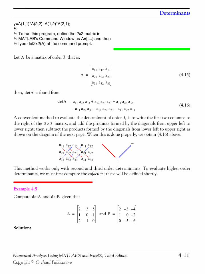
Numerical Analysis Using MATLAB® and Excel®, Third Edition 4−11Copyright © Orchard Publications
Determinants
y=A(1,1)*A(2,2)−A(1,2)*A(2,1);% % To run this program, define the 2x2 matrix in% MATLAB's Command Window as A=[....] and then % type det2x2(A) at the command prompt.
Let be a matrix of order 3, that is,
(4.15)
then, is found from
(4.16)
A convenient method to evaluate the determinant of order 3, is to write the first two columns tothe right of the matrix, and add the products formed by the diagonals from upper left tolower right; then subtract the products formed by the diagonals from lower left to upper right asshown on the diagram of the next page. When this is done properly, we obtain (4.16) above.
This method works only with second and third order determinants. To evaluate higher orderdeterminants, we must first compute the cofactors; these will be defined shortly.
Example 4.5
Compute and given that
and
Solution:
A
Aa11 a12 a13
a21 a22 a23
a31 a32 a33
=
detA
detA a11 a22 a33 a12 a23 a31 a11 a22 a33+ +=
a11 a22 a33 a11 a22 a33 a11 a22 a33–––
3 3×
a11 a12 a13
a21 a22 a23
a31 a32 a33
a11 a12
a21 a22
a31 a32 +
−
detA detB
A2 3 51 0 12 1 0
= B2 3– 4–1 0 2–0 5– 6–
=
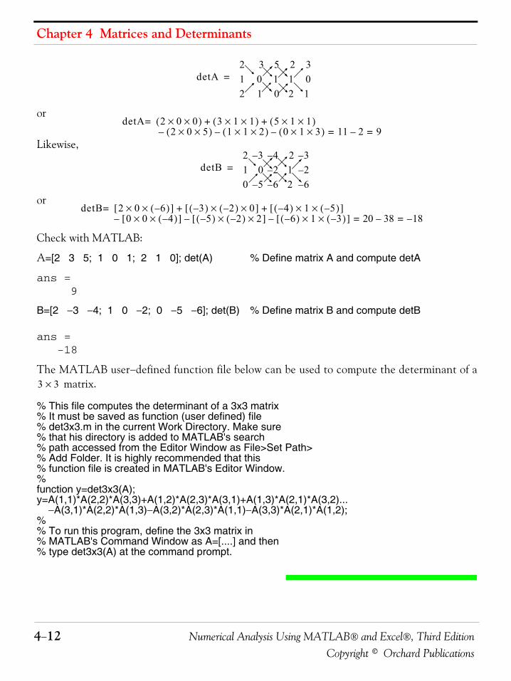
Chapter 4 Matrices and Determinants
4−12 Numerical Analysis Using MATLAB® and Excel®, Third EditionCopyright © Orchard Publications
or
Likewise,
or
Check with MATLAB:
A=[2 3 5; 1 0 1; 2 1 0]; det(A) % Define matrix A and compute detA
ans = 9
B=[2 −3 −4; 1 0 −2; 0 −5 −6]; det(B) % Define matrix B and compute detB
ans = -18
The MATLAB user−defined function file below can be used to compute the determinant of a matrix.
% This file computes the determinant of a 3x3 matrix% It must be saved as function (user defined) file% det3x3.m in the current Work Directory. Make sure% that his directory is added to MATLAB's search% path accessed from the Editor Window as File>Set Path>% Add Folder. It is highly recommended that this % function file is created in MATLAB's Editor Window.%function y=det3x3(A);y=A(1,1)*A(2,2)*A(3,3)+A(1,2)*A(2,3)*A(3,1)+A(1,3)*A(2,1)*A(3,2)... −A(3,1)*A(2,2)*A(1,3)−A(3,2)*A(2,3)*A(1,1)−A(3,3)*A(2,1)*A(1,2);%% To run this program, define the 3x3 matrix in% MATLAB's Command Window as A=[....] and then % type det3x3(A) at the command prompt.
detA2 3 5 2 31 0 1 1 02 1 0 2 1
=
detA 2 0× 0×( ) 3 1× 1×( ) 5 1× 1×( )2 0× 5×( )– 1 1× 2×( ) 0 1× 3×( )––
+ +11 2– 9= =
=
detB2 3– 4– 2 3–1 0 2– 1 2–0 5– 6– 2 6–
=
detB 2 0× 6–( )×[ ] 3–( ) 2–( )× 0×[ ] 4–( ) 1× 5–( )×[ ]0 0× 4–( )×[ ]– 5–( ) 2–( )× 2×[ ] 6–( ) 1× 3–( )×[ ]––
+ +20 38– 18–= =
=
3 3×
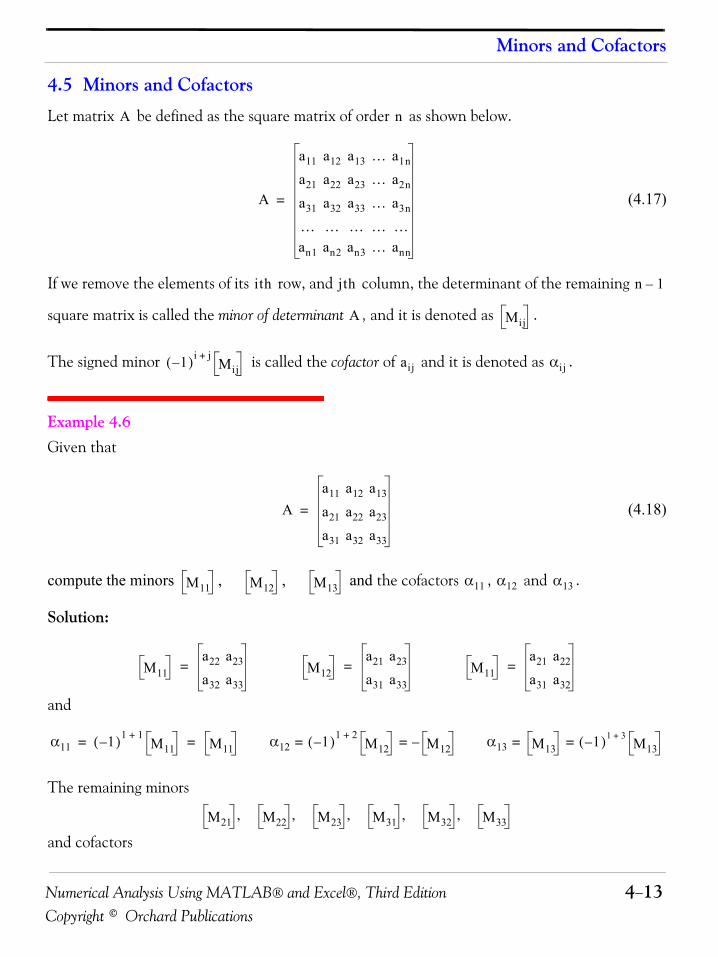
Numerical Analysis Using MATLAB® and Excel®, Third Edition 4−13Copyright © Orchard Publications
Minors and Cofactors
4.5 Minors and Cofactors
Let matrix be defined as the square matrix of order as shown below.
(4.17)
If we remove the elements of its row, and column, the determinant of the remaining
square matrix is called the minor of determinant , and it is denoted as .
The signed minor is called the cofactor of and it is denoted as .
Example 4.6 Given that
(4.18)
compute the minors , , and the cofactors , and .
Solution:
and
The remaining minors
and cofactors
A n
A
a11 a12 a13 … a1n
a21 a22 a23 … a2n
a31 a32 a33 … a3n
… … … … …an1 an2 an3 … ann
=
ith jth n 1–
A Mij
1–( )i j+Mij aij αij
Aa11 a12 a13
a21 a22 a23
a31 a32 a33
=
M11 M12 M13 α11 α12 α13
M11a22 a23
a32 a33
= M12a21 a23
a31 a33
= M11a21 a22
a31 a32
=
α11 1–( )1 1+M11 M11 α12 1–( )1 2+
M12 M12 α13 M13 1–( )1 3+M13= =–= == =
M21 M22 M23 M31 M32 M33, , , , ,
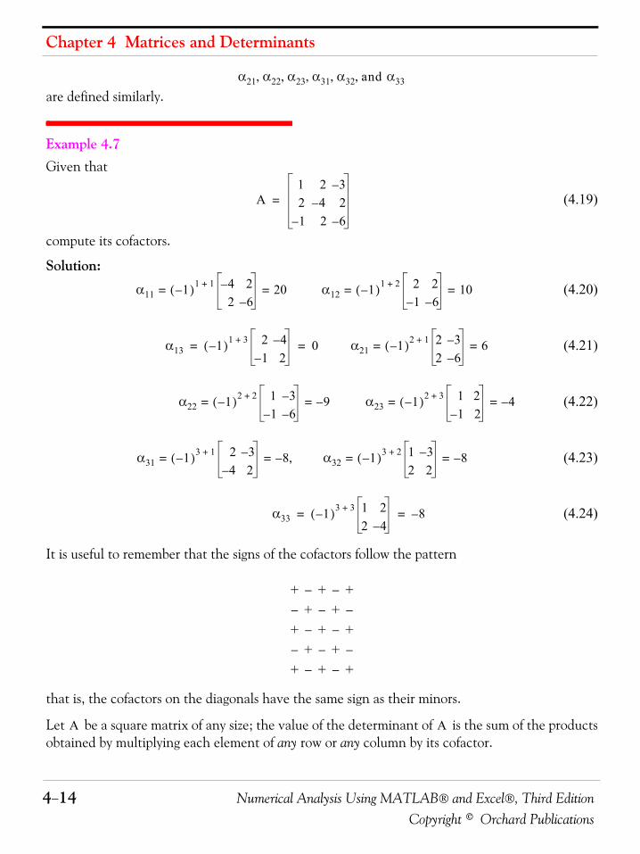
Chapter 4 Matrices and Determinants
4−14 Numerical Analysis Using MATLAB® and Excel®, Third EditionCopyright © Orchard Publications
are defined similarly.
Example 4.7 Given that
(4.19)
compute its cofactors.
Solution:
(4.20)
(4.21)
(4.22)
(4.23)
(4.24)
It is useful to remember that the signs of the cofactors follow the pattern
that is, the cofactors on the diagonals have the same sign as their minors.
Let be a square matrix of any size; the value of the determinant of is the sum of the productsobtained by multiplying each element of any row or any column by its cofactor.
α21 α22 α23 α31 α32 and α33, , , , ,
A1 2 3–2 4– 21– 2 6–
=
α11 1–( )1 1+ 4– 22 6–
20= = α12 1–( )1 2+ 2 21– 6–
10= =
α13 1–( )1 3+ 2 4–1– 2
0 α21 1–( )2 1+ 2 3–2 6–
6= == =
α22 1–( )2 2+ 1 3–1– 6–
9–= = α23 1–( )2 3+ 1 21– 2
4–= =
α31 1–( )3 1+ 2 3–4– 2
8–= = α32 1–( )3 2+ 1 3–2 2
8–= =,
α33 1–( )3 3+ 1 22 4–
8–= =
+ − + − +− + − + −+ − + − +− + − + −+ − + − +
A A
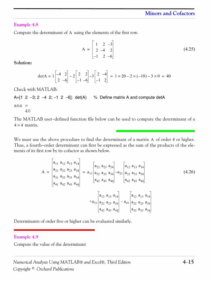
Numerical Analysis Using MATLAB® and Excel®, Third Edition 4−15Copyright © Orchard Publications
Minors and Cofactors
Example 4.8
Compute the determinant of using the elements of the first row.
(4.25)
Solution:
Check with MATLAB:
A=[1 2 −3; 2 −4 2; −1 2 −6]; det(A) % Define matrix A and compute detA
ans = 40
The MATLAB user−defined function file below can be used to compute the determinant of a matrix.
We must use the above procedure to find the determinant of a matrix of order 4 or higher.Thus, a fourth−order determinant can first be expressed as the sum of the products of the ele-ments of its first row by its cofactor as shown below.
(4.26)
Determinants of order five or higher can be evaluated similarly.
Example 4.9 Compute the value of the determinant
A
A1 2 3–2 4– 21– 2 6–
=
detA 1 4– 22 6–
= 2 2 21– 6–
3 2 4–1– 2
–– 1 20× 2 10–( )× 3 0×–– 40= =
4 4×
A
A
a11 a12 a13 a14
a21 a22 a23 a24
a31 a32 a33 a34
a41 a42 a43 a44
a11
a22 a23 a24
a32 a33 a34
a42 a43 a44
a21
a12 a13 a14
a32 a33 a34
a42 a43 a44
–
+a31
a12 a13 a14
a22 a23 a24
a42 a43 a44
a41
a12 a13 a14
a22 a23 a24
a32 a33 a34
–
= =
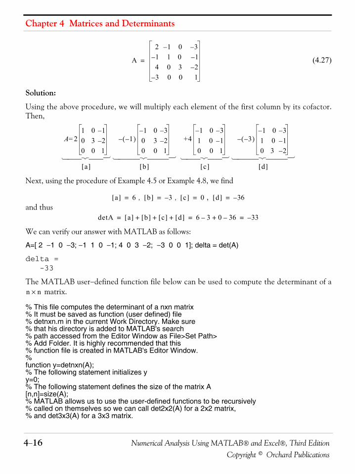
Chapter 4 Matrices and Determinants
4−16 Numerical Analysis Using MATLAB® and Excel®, Third EditionCopyright © Orchard Publications
(4.27)
Solution:
Using the above procedure, we will multiply each element of the first column by its cofactor.Then,
Next, using the procedure of Example 4.5 or Example 4.8, we find
, , , and thus
We can verify our answer with MATLAB as follows:
A=[ 2 −1 0 −3; −1 1 0 −1; 4 0 3 −2; −3 0 0 1]; delta = det(A)
delta = -33
The MATLAB user−defined function file below can be used to compute the determinant of a matrix.
% This file computes the determinant of a nxn matrix% It must be saved as function (user defined) file% detnxn.m in the current Work Directory. Make sure% that his directory is added to MATLAB's search% path accessed from the Editor Window as File>Set Path>% Add Folder. It is highly recommended that this % function file is created in MATLAB's Editor Window.% function y=detnxn(A);% The following statement initializes yy=0;% The following statement defines the size of the matrix A[n,n]=size(A);% MATLAB allows us to use the user-defined functions to be recursively % called on themselves so we can call det2x2(A) for a 2x2 matrix,% and det3x3(A) for a 3x3 matrix.
A
2 1– 0 3–1– 1 0 1–4 0 3 2–3– 0 0 1
=
A=21 0 1–0 3 2–0 0 1
a[ ]
1–( )1– 0 3–
0 3 2–0 0 1
–
b[ ]
+4
1– 0 3–1 0 1–0 0 1
c[ ]
3–( )1– 0 3–
1 0 1–0 3 2–
–
d[ ]
⎧ ⎪ ⎪ ⎨ ⎪ ⎪ ⎩ ⎧ ⎪ ⎪ ⎪ ⎨ ⎪ ⎪ ⎪ ⎩ ⎧ ⎪ ⎪ ⎨ ⎪ ⎪ ⎩ ⎧ ⎪ ⎪ ⎪ ⎨ ⎪ ⎪ ⎪ ⎩
a[ ] 6= b[ ] 3–= c[ ] 0= d[ ] 36–=
detA a[ ] b[ ] c[ ] d[ ]+ + + 6 3– 0 36–+ 33–= = =
n n×
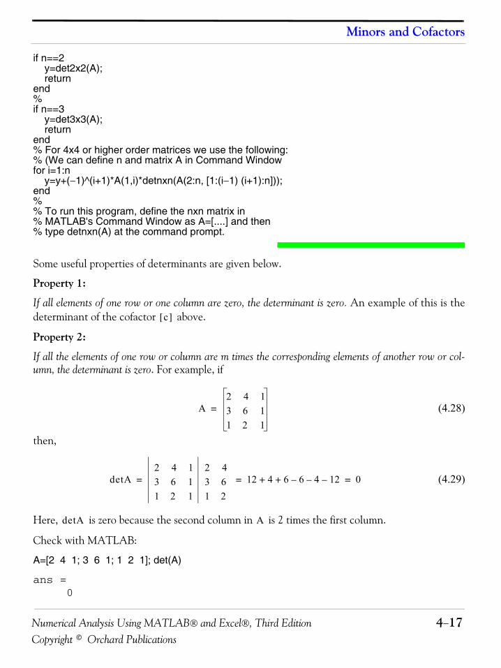
Numerical Analysis Using MATLAB® and Excel®, Third Edition 4−17Copyright © Orchard Publications
Minors and Cofactors
if n==2 y=det2x2(A); returnend%if n==3 y=det3x3(A); returnend% For 4x4 or higher order matrices we use the following:% (We can define n and matrix A in Command Windowfor i=1:n y=y+(−1)^(i+1)*A(1,i)*detnxn(A(2:n, [1:(i−1) (i+1):n]));end%% To run this program, define the nxn matrix in% MATLAB's Command Window as A=[....] and then % type detnxn(A) at the command prompt.
Some useful properties of determinants are given below.
Property 1:
If all elements of one row or one column are zero, the determinant is zero. An example of this is thedeterminant of the cofactor above.
Property 2:
If all the elements of one row or column are m times the corresponding elements of another row or col-umn, the determinant is zero. For example, if
(4.28)
then,
(4.29)
Here, is zero because the second column in is 2 times the first column.
Check with MATLAB:
A=[2 4 1; 3 6 1; 1 2 1]; det(A)
ans = 0
c[ ]
A2 4 13 6 11 2 1
=
detA2 4 13 6 11 2 1
2 43 61 2
12 4 6 6 4–– 12–+ + 0= = =
detA A
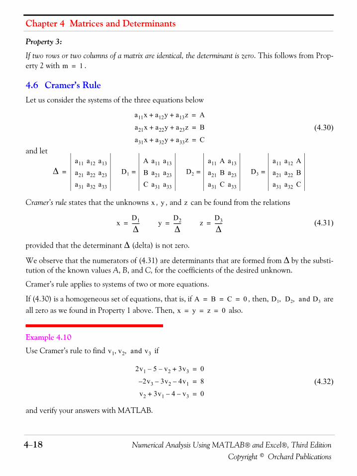
Chapter 4 Matrices and Determinants
4−18 Numerical Analysis Using MATLAB® and Excel®, Third EditionCopyright © Orchard Publications
Property 3:
If two rows or two columns of a matrix are identical, the determinant is zero. This follows from Prop-erty 2 with .
4.6 Cramer’s RuleLet us consider the systems of the three equations below
(4.30)
and let
Cramer’s rule states that the unknowns , , and can be found from the relations
(4.31)
provided that the determinant Δ (delta) is not zero.
We observe that the numerators of (4.31) are determinants that are formed from Δ by the substi-tution of the known values A, B, and C, for the coefficients of the desired unknown.
Cramer’s rule applies to systems of two or more equations.
If (4.30) is a homogeneous set of equations, that is, if , then, areall zero as we found in Property 1 above. Then, also.
Example 4.10
Use Cramer’s rule to find if
(4.32)
and verify your answers with MATLAB.
m 1=
a11x a12y a13z+ + A=
a21x a22y a23z+ + B=
a31x a32y a33z+ + C=
Δa11 a12 a13
a21 a22 a23
a31 a32 a33
D1
A a11 a13
B a21 a23
C a31 a33
D2
a11 A a13
a21 B a23
a31 C a33
D3
a11 a12 Aa21 a22 Ba31 a32 C
====
x y z
xD1
Δ------= y
D2
Δ------= z
D3
Δ------=
A B C 0= = = D1 D2 and D3, ,x y z 0= = =
v1 v2 and v3, ,
2v1 5– v2– 3v3+ 0=
2v3 3v2 4v1––– 8=
v2 3v1 4– v3–+ 0=
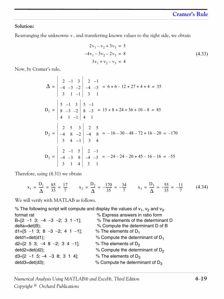
Numerical Analysis Using MATLAB® and Excel®, Third Edition 4−19Copyright © Orchard Publications
Cramer’s Rule
Solution:
Rearranging the unknowns , and transferring known values to the right side, we obtain
(4.33)
Now, by Cramer’s rule,
Therefore, using (4.31) we obtain
(4.34)
We will verify with MATLAB as follows.
% The following script will compute and display the values of v1, v2 and v3.format rat % Express answers in ratio formB=[2 −1 3; −4 −3 −2; 3 1 −1]; % The elements of the determinant Ddelta=det(B); % Compute the determinant D of Bd1=[5 −1 3; 8 −3 −2; 4 1 −1]; % The elements of D1detd1=det(d1); % Compute the determinant of D1d2=[2 5 3; −4 8 −2; 3 4 −1]; % The elements of D2detd2=det(d2); % Compute the determinant of D2d3=[2 −1 5; −4 −3 8; 3 1 4]; % The elements of D3detd3=det(d3); % Compute he determinant of D3
v
2v1 v2– 3v3+ 5=
4v1 3v2 2v3––– 8=
3v1 v2 v3–+ 4=
Δ2 1– 34– 3– 2–3 1 1–
2 1–4– 3–3 1
6 6 12– 27 4 4+ + + + 35= = =
D1
5 1– 38 3– 2–4 1 1–
5 1–8 3–4 1
15 8 24 36 10 8–+ + + + 85= = =
D2
2 5 34– 8 2–3 4 1–
2 54– 83 4
16– 30– 48– 72– 16 20–+ 170–= = =
D3
2 1– 54– 3– 83 1 4
2 1–4– 3–3 1
24– 24– 20– 45 16– 16–+ 55–= = =
x1D1
Δ------ 85
35------ 17
7------= = = x2
D2
Δ------ 170
35---------– 34
7------–= = = x3
D3
Δ------ 55
35------– 11
7------–= = =
Chapter 4 Matrices and Determinants
4−20 Numerical Analysis Using MATLAB® and Excel®, Third EditionCopyright © Orchard Publications
v1=detd1/delta; % Compute the value of v1v2=detd2/delta; % Compute the value of v2v3=detd3/delta; % Compute the value of v3%disp('v1=');disp(v1); % Display the value of v1disp('v2=');disp(v2); % Display the value of v2disp('v3=');disp(v3); % Display the value of v3
v1= 17/7v2= -34/7 v3= -11/7
These are the same values as in (4.34)
4.7 Gaussian Elimination MethodWe can find the unknowns in a system of two or more equations also by the Gaussian eliminationmethod. With this method, the objective is to eliminate one unknown at a time. This can be doneby multiplying the terms of any of the equations of the system by a number such that we can add(or subtract) this equation to another equation in the system so that one of the unknowns will beeliminated. Then, by substitution to another equation with two unknowns, we can find the sec-ond unknown. Subsequently, substitution of the two values found can be made into an equationwith three unknowns from which we can find the value of the third unknown. This procedure isrepeated until all unknowns are found. This method is best illustrated with the following examplewhich consists of the same equations as the previous example.
Example 4.11
Use the Gaussian elimination method to find of
(4.35)
Solution:
As a first step, we add the first equation of (4.35) with the third to eliminate the unknown andwe obtain the following equation.
v1 v2 and v3, ,
2v1 v2– 3v3+ 5=
4v1 3v2 2v3––– 8=
3v1 v2 v3–+ 4=
v2
Numerical Analysis Using MATLAB® and Excel®, Third Edition 4−21Copyright © Orchard Publications
The Adjoint of a Matrix
(4.36)
Next, we multiply the third equation of (4.35) by 3, and we add it with the second to eliminate. Then, we obtain the following equation.
(4.37)
Subtraction of (4.37) from (4.36) yields
(4.38)
Now, we can find the unknown from either (4.36) or (4.37). By substitution of (4.38) into(4.36) we obtain
(4.39)
Finally, we can find the last unknown from any of the three equations of (4.35). By substitu-tion into the first equation we obtain
(4.40)
These are the same values as those we found in Example 4.10.
The Gaussian elimination method works well if the coefficients of the unknowns are small inte-gers, as in Example 4.11. However, it becomes impractical if the coefficients are large or fractionalnumbers.
The Gaussian elimination is further discussed in Chapter 14 in conjunction with the factor-ization method.
4.8 The Adjoint of a Matrix
Let us assume that is an square matrix and is the cofactor of . Then the adjoint of ,denoted as , is defined as the square matrix shown on the next page.
5v1 2v3+ 9=
v2
5v1 5v3– 20=
7v3 11 or v3117
------–=–=
v1
5v1 2 117
------–⎝ ⎠⎛ ⎞⋅+ 9 or v1
177
------==
v2
v2 2v1 3v3 5–+ 347------ 33
7------– 35
7------– 34
7------–= = =
LU
A n αij aij A
adjA n
Chapter 4 Matrices and Determinants
4−22 Numerical Analysis Using MATLAB® and Excel®, Third EditionCopyright © Orchard Publications
(4.41)
We observe that the cofactors of the elements of the row (column) of , are the elements ofthe column (row) of .
Example 4.12
Compute given that
(4.42)
Solution:
4.9 Singular and Non−Singular Matrices
An square matrix is called singular if ; if , A is called non−singular. If an square matrix is nearly singular, that is, if the determinant of that matrix is very small, thematrix is said to be ill−conditioned. This topic is discussed in Appendix C.
Example 4.13 Given that
adjA
α11 α21 α31 … αn1
α12 α22 α32 … αn2
α13 α23 α33 … αn3
… … … … …α1n α2n α3n … αnn
=
ith Aith adjA
adjA
A1 2 31 3 41 4 3
=
adjA
3 44 3
2 34 3
– 2 33 4
1 41 3
– 1 31 3
2 33 4
–
1 31 4
1 21 4
– 1 21 3
7– 6 1–1 0 1–1 2– 1
= =
n A detA 0= detA 0≠ nA
Numerical Analysis Using MATLAB® and Excel®, Third Edition 4−23Copyright © Orchard Publications
The Inverse of a Matrix
(4.43)
determine whether this matrix is singular or non−singular.
Solution:
Therefore, matrix is singular.
4.10 The Inverse of a Matrix
If and B are square matrices such that , where is the identity matrix, is
called the inverse of , denoted as , and likewise, is called the inverse of , that is,
If a matrix is non−singular, we can compute its inverse from the relation
(4.44)
Example 4.14 Given that
(4.45)
compute its inverse, that is, find
Solution:
Here, , and since this is a non−zero value, it is possible tocompute the inverse of using (4.44).From Example 4.12,
A1 2 32 3 43 5 7
=
detA1 2 32 3 43 5 7
1 22 33 5
21 24 30 27– 20– 28–+ + 0= = =
A
A n AB BA I= = I B
A B A 1–= A B
A B 1–=
A
A 1– 1detA------------adjA=
A1 2 31 3 41 4 3
=
A 1–
detA 9 8 12 9– 16– 6–+ + 2–= =
A
Chapter 4 Matrices and Determinants
4−24 Numerical Analysis Using MATLAB® and Excel®, Third EditionCopyright © Orchard Publications
Then,
(4.46)
Check with MATLAB:
A=[1 2 3; 1 3 4; 1 4 3], invA=inv(A) % Define matrix A and compute its inverse
A = 1 2 3 1 3 4 1 4 3
invA = 3.5000 -3.0000 0.5000 -0.5000 0 0.5000 -0.5000 1.0000 -0.5000
Multiplication of a matrix by its inverse produces the identity matrix , that is,
(4.47)
Example 4.15 Prove the validity of (4.47) for
Proof:
Then,
and
adjA7– 6 1–
1 0 1–1 2– 1
=
A 1– 1detA------------adjA 1
2–------
7– 6 1–1 0 1–1 2– 1
3.5 3– 0.50.5– 0 0.50.5– 1 0.5–
= = =
A A 1– I
AA 1– I or A 1– A I ==
A 4 32 2
=
detA 8 6– 2 and adjA 2 3–2– 4
== =
A 1– 1detA------------adjA 1
2--- 2 3–
2– 41 3– 2⁄1– 2
= = =
Numerical Analysis Using MATLAB® and Excel®, Third Edition 4−25Copyright © Orchard Publications
Solution of Simultaneous Equations with Matrices
4.11 Solution of Simultaneous Equations with MatricesConsider the relation
(4.48)
where and are matrices whose elements are known, and is a matrix (a column vector)whose elements are the unknowns. We assume that and are conformable for multiplication.
Multiplication of both sides of (4.48) by yields:
(4.49)or
(4.50)
Therefore, we can use (4.50) to solve any set of simultaneous equations that have solutions. Wewill refer to this method as the inverse matrix method of solution of simultaneous equations.
Example 4.16 Given the system of equations
(4.51)
compute the unknowns using the inverse matrix method.
Solution:
In matrix form, the given set of equations is where
(4.52)
Then,
AA 1– 4 32 2
1 3– 2⁄1– 2
4 3– 6– 6+2 2– 3– 4+
1 00 1
I= = = =
AX B=
A B XA X
A 1–
A 1– AX A 1– B IX A 1– B= = =
X=A 1– B
2x1 3x2 x3+ + 9=
x1 2x2 3x3+ + 6=
3x1 x2 2x3+ + 8=⎩ ⎭⎪ ⎪⎨ ⎬⎪ ⎪⎧ ⎫
x1 x2 and x3, ,
AX B=
A2 3 11 2 33 1 2
= Xx1
x2
x3
= B968
=, ,
Chapter 4 Matrices and Determinants
4−26 Numerical Analysis Using MATLAB® and Excel®, Third EditionCopyright © Orchard Publications
(4.53)or
(4.54)
Next, we find the determinant , and the adjoint .
Therefore,
and by (4.53) we obtain the solution as follows.
(4.55)
To verify our results, we could use the MATLAB inv(A) function, and multiply by . How-ever, it is easier to use the matrix left division operation ; this is MATLAB’s solution of
for the matrix equation , where matrix is the same size as matrix . For thisexample,
A=[2 3 1; 1 2 3; 3 1 2]; B=[9 6 8]'; X=A \ B % Observe that B is a column vector
X = 1.9444 1.6111 0.2778
As stated earlier, while MATLAB has the built−in function det(A) for computing the determi-nant of a matrix A, this function is not included in the MATLAB Run−Time Function LibraryList that is used with the Simulink Embedded MATLAB Function block. The MATLAB user−defined function file below can be used to compute the determinant of a matrix. A user-defined function to compute the inverse of an is presented in Chapter 14.
X A 1– B=
x1
x2
x3
2 3 11 2 33 1 2
1–968
=
detA adjA
detA 18= and adjA1 5– 77 1 5–5– 7 1
=
A 1– 1detA------------ adjA 1
18------
1 5– 77 1 5–5– 7 1
= =
Xx1
x2
x3
118------
1 5– 77 1 5–5– 7 1
968
118------
35295
35 18⁄29 18⁄5 18⁄
1.941.610.28
= = = = =
A 1– BX A \ B=
A 1– B A X⋅ B= X B
2 2×n n×
Numerical Analysis Using MATLAB® and Excel®, Third Edition 4−27Copyright © Orchard Publications
Solution of Simultaneous Equations with Matrices
Example 4.17 For the electric circuit of Figure 4.1, the mesh equations are
Figure 4.1. Circuit for Example 4.17
(4.56)
Use the inverse matrix method to compute the values of the currents .
Solution:
For this example, the matrix equation is or , where
The next step is to find . This is found from the relation
(4.57)
Therefore, we find the determinant and the adjoint of . For this example, we find that
(4.58)
Then,
and
+−
V = 100 v
9 Ω 9 Ω 4 Ω
2 Ω2 Ω1 Ω
I1 I3I2
10I1 9I2– 100=
9I1 20I2 9I3–+– 0=
9I2 15I3+– 0=
I1 I2 and I3, ,
RI V = I R 1– V=
R10 9– 0
9– 20 9–0 9– 15
= V100
00
and II1
I2
I3
==,
R 1–
R 1– 1detR------------ adjR=
R
detR 975= adjR219 135 81135 150 9081 90 119
=,
R 1– 1detR------------adjR 1
975---------
219 135 81135 150 9081 90 119
= =
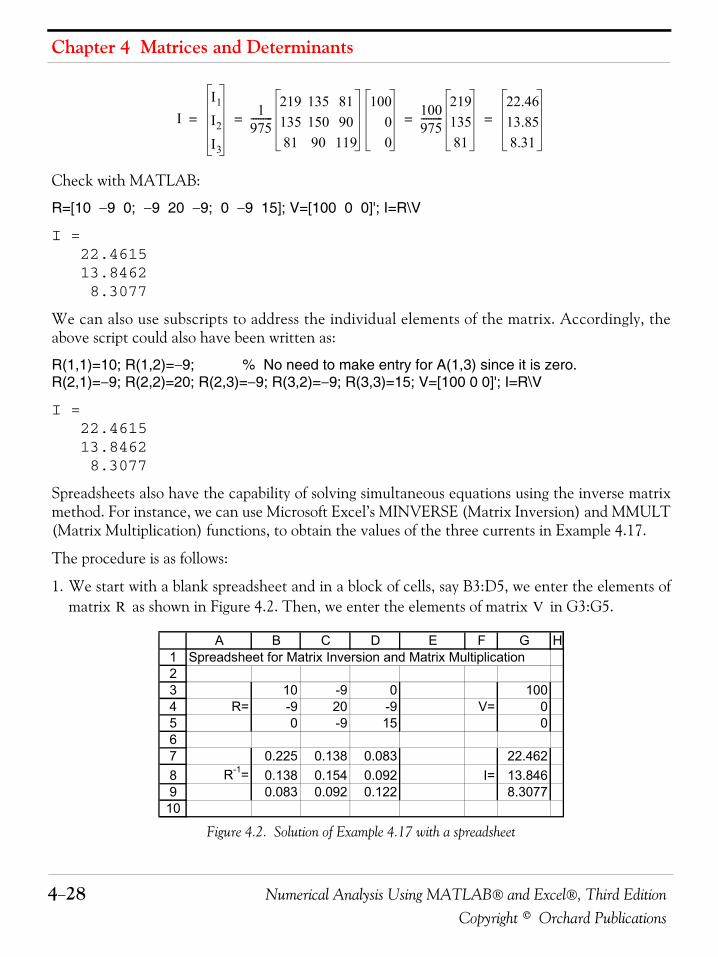
Chapter 4 Matrices and Determinants
4−28 Numerical Analysis Using MATLAB® and Excel®, Third EditionCopyright © Orchard Publications
Check with MATLAB:
R=[10 −9 0; −9 20 −9; 0 −9 15]; V=[100 0 0]'; I=R\V
I = 22.4615 13.8462 8.3077
We can also use subscripts to address the individual elements of the matrix. Accordingly, theabove script could also have been written as:
R(1,1)=10; R(1,2)=−9; % No need to make entry for A(1,3) since it is zero.R(2,1)=−9; R(2,2)=20; R(2,3)=−9; R(3,2)=−9; R(3,3)=15; V=[100 0 0]'; I=R\V
I = 22.4615 13.8462 8.3077
Spreadsheets also have the capability of solving simultaneous equations using the inverse matrixmethod. For instance, we can use Microsoft Excel’s MINVERSE (Matrix Inversion) and MMULT(Matrix Multiplication) functions, to obtain the values of the three currents in Example 4.17.
The procedure is as follows:
1. We start with a blank spreadsheet and in a block of cells, say B3:D5, we enter the elements ofmatrix as shown in Figure 4.2. Then, we enter the elements of matrix in G3:G5.
Figure 4.2. Solution of Example 4.17 with a spreadsheet
II1
I2
I3
1975---------
219 135 81135 150 9081 90 119
10000
100975---------
21913581
22.4613.858.31
= = = =
R V
12345678910
A B C D E F G HSpreadsheet for Matrix Inversion and Matrix Multiplication
10 -9 0 100R= -9 20 -9 V= 0
0 -9 15 0
0.225 0.138 0.083 22.462R-1= 0.138 0.154 0.092 I= 13.846
0.083 0.092 0.122 8.3077
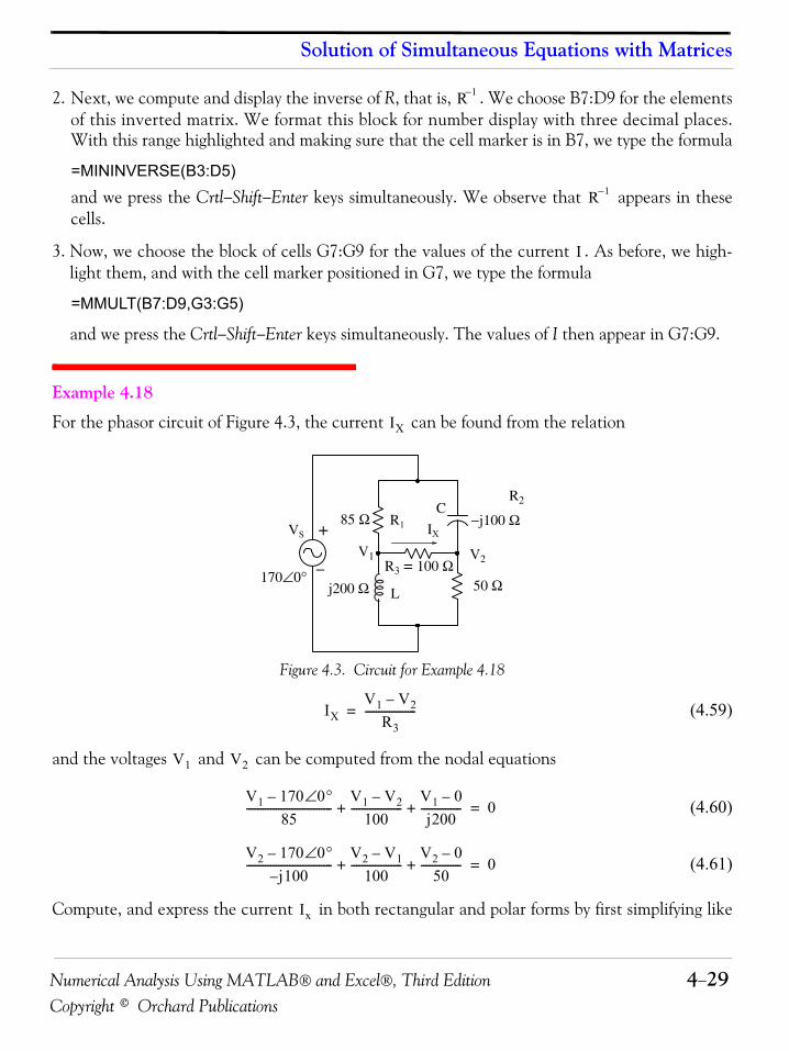
Numerical Analysis Using MATLAB® and Excel®, Third Edition 4−29Copyright © Orchard Publications
Solution of Simultaneous Equations with Matrices
2. Next, we compute and display the inverse of R, that is, . We choose B7:D9 for the elementsof this inverted matrix. We format this block for number display with three decimal places.With this range highlighted and making sure that the cell marker is in B7, we type the formula
=MININVERSE(B3:D5)and we press the Crtl−Shift−Enter keys simultaneously. We observe that appears in thesecells.
3. Now, we choose the block of cells G7:G9 for the values of the current . As before, we high-light them, and with the cell marker positioned in G7, we type the formula
=MMULT(B7:D9,G3:G5)
and we press the Crtl−Shift−Enter keys simultaneously. The values of I then appear in G7:G9.
Example 4.18
For the phasor circuit of Figure 4.3, the current can be found from the relation
Figure 4.3. Circuit for Example 4.18
(4.59)
and the voltages and can be computed from the nodal equations
(4.60)
(4.61)
Compute, and express the current in both rectangular and polar forms by first simplifying like
R 1–
R 1–
I
IX
+
−
R185 Ω
50 Ω
R2C
L
R3 = 100 Ω
IXVS−j100 Ω
j200 Ω170∠0°
V1 V2
IXV1 V2–
R3-------------------=
V1 V2
V1 170 0°∠–
85--------------------------------
V1 V2–
100-------------------
V1 0–
j200---------------+ + 0=
V2 170 0°∠–
j100–--------------------------------
V2 V1–
100-------------------
V2 0–
50---------------+ + 0=
Ix
Chapter 4 Matrices and Determinants
4−30 Numerical Analysis Using MATLAB® and Excel®, Third EditionCopyright © Orchard Publications
terms, collecting, and then writing the above relations in matrix form as , where, , and .
Solution:
The elements of the matrix are the coefficients of and . Simplifying and rearranging the
nodal equations of (4.60) and (4.61), we obtain
Next, we write (4.62) in matrix form as
(4.62)
where the matrices , , and are as indicatedin (4.63).
We will use MATLAB to compute the voltages and , and to do all other computations.The script is shown below.
Y=[0.0218−0.005j −0.01; −0.01 0.03+0.01j]; I=[2; 1.7j]; V=Y\I; % Define Y, I, and find Vfprintf('\n'); % Insert a line disp(' V1 V2'); disp(' ------------------'); % Display V1 and V2 with dash line underneathfprintf('%9.3f %9.3f\n',V(1),V(2)) % Display values of V1 and V2 in tabular formfprintf('\n')% Insert another line
V1 V2 ------------------ 104.905 53.416
Next, we find from
R3=100; IX=(V(1)−V(2))/R3 % Compute the value of IX
IX = 0.5149 - 0.0590i
and this is the rectangular form of . For the polar form we use
magIX=abs(IX) % Compute the magnitude of IX
magIX =
YV I=
Y admit cetan= V voltage= I current=
Y V1 V2
0.0218 j0.005–( )V1 0.01V2– 2=
0.01– V1 0.03 j0.01+( )V2+ j1.7=
0.0218 j0.005– 0.01–0.01– 0.03 j0.01+
Y
V1
V2
V
2j1.7
I
=
⎧ ⎪ ⎪ ⎪ ⎪ ⎪ ⎨ ⎪ ⎪ ⎪ ⎪ ⎪ ⎩ ⎧ ⎨ ⎩ ⎧ ⎨ ⎩
Y V I
V1 V2
IX
IX
Numerical Analysis Using MATLAB® and Excel®, Third Edition 4−31Copyright © Orchard Publications
Solution of Simultaneous Equations with Matrices
0.5183
thetaIX=angle(IX)*180/pi % Compute angle theta in degrees
thetaIX = -6.5326
Therefore, in polar form
Spreadsheets have limited capabilities with complex numbers, and thus we cannot use them tocompute matrices that include complex numbers in their elements.
IX 0.518 6.53°–∠=
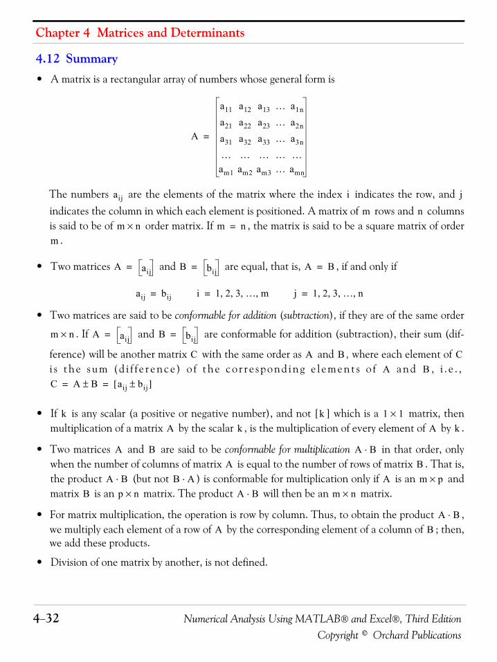
Chapter 4 Matrices and Determinants
4−32 Numerical Analysis Using MATLAB® and Excel®, Third EditionCopyright © Orchard Publications
4.12 Summary• A matrix is a rectangular array of numbers whose general form is
The numbers are the elements of the matrix where the index indicates the row, and indicates the column in which each element is positioned. A matrix of rows and columnsis said to be of order matrix. If , the matrix is said to be a square matrix of order
.
• Two matrices and are equal, that is, , if and only if
• Two matrices are said to be conformable for addition (subtraction), if they are of the same order
. If and are conformable for addition (subtraction), their sum (dif-
ference) will be another matrix with the same order as and , where each element of i s t h e s u m ( d i f f e r e n c e ) o f t h e c o r r e s po n d i n g e l eme n t s o f a n d , i . e . ,
• If is any scalar (a positive or negative number), and not [ ] which is a matrix, thenmultiplication of a matrix by the scalar , is the multiplication of every element of by .
• Two matrices and are said to be conformable for multiplication in that order, onlywhen the number of columns of matrix is equal to the number of rows of matrix . That is,the product (but not ) is conformable for multiplication only if is an andmatrix is an matrix. The product will then be an matrix.
• For matrix multiplication, the operation is row by column. Thus, to obtain the product ,we multiply each element of a row of by the corresponding element of a column of ; then,we add these products.
• Division of one matrix by another, is not defined.
A
a11 a12 a13 … a1n
a21 a22 a23 … a2n
a31 a32 a33 … a3n
… … … … …am1 am2 am3 … amn
=
aij i j
m nm n× m n=
m
A aij= B bij= A B=
aij bij= i 1 2 3 … m, , , ,= j 1 2 3 … n, , , ,=
m n× A aij= B bij=
C A B CA B
C A B± aij bij±[ ]= =
k k 1 1×A k A k
A B A B⋅A B
A B⋅ B A⋅ A m p×B p n× A B⋅ m n×
A B⋅A B
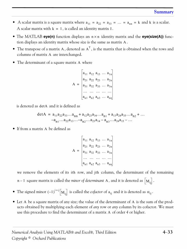
Numerical Analysis Using MATLAB® and Excel®, Third Edition 4−33Copyright © Orchard Publications
Summary
• A scalar matrix is a square matrix where and is a scalar. A scalar matrix with , is called an identity matrix .
• The MATLAB eye(n) function displays an identity matrix and the eye(size(A)) func-tion displays an identity matrix whose size is the same as matrix .
• The transpose of a matrix , denoted as , is the matrix that is obtained when the rows andcolumns of matrix are interchanged.
• The determinant of a square matrix where
is denoted as and it is defined as
• If from a matrix be defined as
we remove the elements of its row, and column, the determinant of the remaining
square matrix is called the minor of determinant , and it is denoted as .
• The signed minor is called the cofactor of and it is denoted as .
• Let be a square matrix of any size; the value of the determinant of is the sum of the prod-ucts obtained by multiplying each element of any row or any column by its cofactor. We mustuse this procedure to find the determinant of a matrix of order 4 or higher.
a11 a22 a33 … ann k= = = = = k
k 1= I
n n×A
A AT
A
A
A
a11 a12 a13 … a1n
a21 a22 a23 … a2n
a31 a32 a33 … a3n
… … … … …an1 an2 an3 … ann
=
detA
detA a11a22a33…ann a12a23a34…an1 a13a24a35…an2 … an1…a22a13… an2– …a23a14 an3…a24a15 …–––
+ + +=
A
A
a11 a12 a13 … a1n
a21 a22 a23 … a2n
a31 a32 a33 … a3n
… … … … …an1 an2 an3 … ann
=
ith jth
n 1– A Mij
1–( )i j+Mij aij αij
A A
A
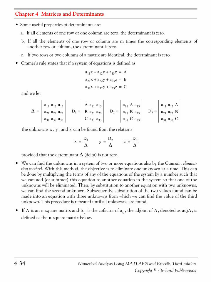
Chapter 4 Matrices and Determinants
4−34 Numerical Analysis Using MATLAB® and Excel®, Third EditionCopyright © Orchard Publications
• Some useful properties of determinants are:
a. If all elements of one row or one column are zero, the determinant is zero.
b. If all the elements of one row or column are m times the corresponding elements ofanother row or column, the determinant is zero.
c. If two rows or two columns of a matrix are identical, the determinant is zero.
• Cramer’s rule states that if a system of equations is defined as
and we let
the unknowns , , and can be found from the relations
provided that the determinant Δ (delta) is not zero.
• We can find the unknowns in a system of two or more equations also by the Gaussian elimina-tion method. With this method, the objective is to eliminate one unknown at a time. This canbe done by multiplying the terms of any of the equations of the system by a number such thatwe can add (or subtract) this equation to another equation in the system so that one of theunknowns will be eliminated. Then, by substitution to another equation with two unknowns,we can find the second unknown. Subsequently, substitution of the two values found can bemade into an equation with three unknowns from which we can find the value of the thirdunknown. This procedure is repeated until all unknowns are found.
• If is an square matrix and is the cofactor of , the adjoint of , denoted as , isdefined as the square matrix below.
a11x a12y a13z+ + A=
a21x a22y a23z+ + B=
a31x a32y a33z+ + C=
Δa11 a12 a13
a21 a22 a23
a31 a32 a33
D1
A a11 a13
B a21 a23
C a31 a33
D2
a11 A a13
a21 B a23
a31 C a33
D3
a11 a12 Aa21 a22 Ba31 a32 C
====
x y z
xD1
Δ------= y
D2
Δ------= z
D3
Δ------=
A n αij aij A adjA
n
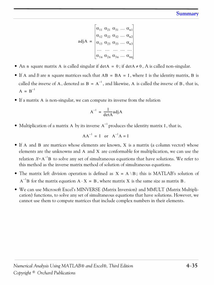
Numerical Analysis Using MATLAB® and Excel®, Third Edition 4−35Copyright © Orchard Publications
Summary
• An square matrix is called singular if ; if , A is called non-singular.
• If and B are square matrices such that , where is the identity matrix, is
called the inverse of , denoted as , and likewise, is called the inverse of , that is,
• If a matrix is non-singular, we can compute its inverse from the relation
• Multiplication of a matrix by its inverse produces the identity matrix , that is,
• If and are matrices whose elements are known, is a matrix (a column vector) whoseelements are the unknowns and and are conformable for multiplication, we can use the
relation to solve any set of simultaneous equations that have solutions. We refer tothis method as the inverse matrix method of solution of simultaneous equations.
• The matrix left division operation is defined as ; this is MATLAB’s solution of
for the matrix equation , where matrix is the same size as matrix .
• We can use Microsoft Excel’s MINVERSE (Matrix Inversion) and MMULT (Matrix Multipli-cation) functions, to solve any set of simultaneous equations that have solutions. However, wecannot use them to compute matrices that include complex numbers in their elements.
adjA
α11 α21 α31 … αn1
α12 α22 α32 … αn2
α13 α23 α33 … αn3
… … … … …α1n α2n α3n … αnn
=
n A detA 0= detA 0≠
A n AB BA I= = I B
A B A 1–= A B
A B 1–=
A
A 1– 1detA------------adjA=
A A 1– I
AA 1– I or A 1– A I ==
A B XA X
X=A 1– B
X A \ B=
A 1– B A X⋅ B= X B
Chapter 4 Matrices and Determinants
4−36 Numerical Analysis Using MATLAB® and Excel®, Third EditionCopyright © Orchard Publications
4.13 Exercises
For Exercises 1 through 3 below, the matrices , , and are defined as:
1. Perform the following computations, if possible. Verify your answers with Excel or MATLAB.
a. b. c. d. e. f. g. h.
2. Perform the following computations, if possible. Verify your answers with Excel or MATLAB.
a. b. c. d. e. f. g. h.
3. Perform the following computations, if possible. Verify your answers with Excel or MATLAB.
a. b. c. d. e. f.
4. Solve the following system of equations using Cramer’s rule. Verify your answers with Excel orMATLAB.
5. Repeat Exercise 4 using the Gaussian elimination method.
6. Use the MATLAB det(A) function to find the unknowns of the system of equations below.
7. Solve the following system of equations using the inverse matrix method. Verify your answerswith Excel or MATLAB.
A B C D
A1 1– 4–5 7 2–3 5– 6
= B5 9 3–2– 8 27 4– 6
= C=4 63– 85 2–
D 1 2– 33– 6 4–
=
A B+ A C+ B D+ C D+ A B– A C– B D– C D–
A B⋅ A C⋅ B D⋅ C D⋅ B A⋅ C A⋅ D A⋅ D· C⋅
detA detB detC detD det A B⋅( ) det A C⋅( )
x1 2x2 x3+– 4–=
2x– 1 3x2 x3+ + 9=
3x1 4x2 5x3–+ 0=
x1– 2x2 3x3– 5x4+ + 14=
x1 3x2 2x3 x4–+ + 9=
3x1 3– x2 2x3 4x4+ + 19=
4x1 2x2 5x3 x4+ + + 27=
1 3 43 1 2–2 3 5
x1
x2
x3
⋅3–2–0
=

Numerical Analysis Using MATLAB® and Excel®, Third Edition 4−37Copyright © Orchard Publications
Exercises
8. Use Excel to find the unknowns for the system
Verify your answers with the MATLAB left division operation.
2 4 3 2–2 4– 1 31– 3 4– 22 2– 2 1
x1
x2
x3
x4
⋅
11014–7
=
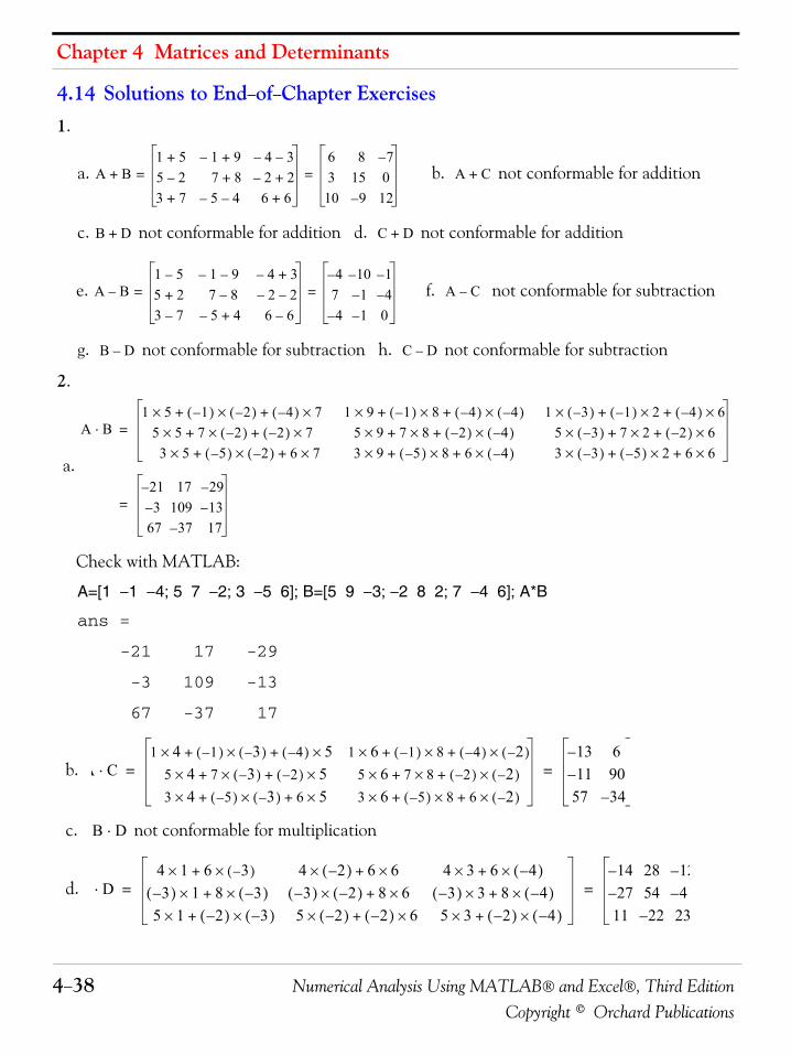
Chapter 4 Matrices and Determinants
4−38 Numerical Analysis Using MATLAB® and Excel®, Third EditionCopyright © Orchard Publications
4.14 Solutions to End−of−Chapter Exercises1.
a. b. not conformable for addition
c. not conformable for addition d. not conformable for addition
e. f. not conformable for subtraction
g. not conformable for subtraction h. not conformable for subtraction
2.
a.
Check with MATLAB:
A=[1 −1 −4; 5 7 −2; 3 −5 6]; B=[5 9 −3; −2 8 2; 7 −4 6]; A*B
ans =
-21 17 -29
-3 109 -13
67 -37 17
b.
c. not conformable for multiplication
d.
A B+1 5+ 1– 9+ 4– 3–5 2– 7 8+ 2– 2+3 7+ 5– 4– 6 6+
6 8 7–3 15 010 9– 12
= = A C+
B D+ C D+
A B–1 5– 1– 9– 4– 3+5 2+ 7 8– 2– 2–3 7– 5– 4+ 6 6–
4– 10– 1–7 1– 4–4– 1– 0
= = A C–
B D– C D–
A B⋅1 5 1–( ) 2–( ) 4–( ) 7×+×+× 1 9 1–( ) 8 4–( ) 4–( )×+×+× 1 3–( ) 1–( ) 2 4–( ) 6×+×+×
5 5 7 2–( ) 2–( ) 7×+×+× 5 9 7 8 2–( ) 4–( )×+×+× 5 3–( ) 7 2 2–( ) 6×+×+×3 5 5–( ) 2–( ) 6 7×+×+× 3 9 5–( ) 8 6 4–( )×+×+× 3 3–( ) 5–( ) 2 6 6×+×+×
=
21– 17 29–3– 109 13–
67 37– 17
=
A C⋅1 4 1–( ) 3–( ) 4–( ) 5×+×+× 1 6 1–( ) 8 4–( ) 2–( )×+×+×
5 4 7 3–( ) 2–( ) 5×+×+× 5 6 7 8 2–( ) 2–( )×+×+×3 4 5–( ) 3–( ) 6 5×+×+× 3 6 5–( ) 8 6 2–( )×+×+×
13– 611– 90
57 34–
= =
B D⋅
D⋅4 1 6 3–( )×+× 4 2–( ) 6 6×+× 4 3 6 4–( )×+×3–( ) 1 8 3–( )×+× 3–( ) 2–( ) 8 6×+× 3–( ) 3 8 4–( )×+×
5 1 2–( ) 3–( )×+× 5 2–( ) 2–( ) 6×+× 5 3 2–( ) 4–( )×+×
14– 28 12–27– 54 41–
11 22– 23
= =
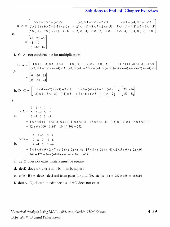
Numerical Analysis Using MATLAB® and Excel®, Third Edition 4−39Copyright © Orchard Publications
Solutions to End−of−Chapter Exercises
e.
f. not conformable for multiplication
g.
h.
3.
a.
b.
c. does not exist; matrix must be square
d. does not exist; matrix must be square
e. and from parts (a) and (b),
f. does not exist because does not exist
B A⋅5 1 9 5 3–( ) 3×+×+× 2–( ) 1 8 5× 2 3×++× 7 1 4–( ) 5 6 3×+×+×
5 1–( ) 9 7 3–( ) 5–( )×+×+× 2–( ) 1–( ) 8 7× 2 5–( )×++× 7 1–( ) 4–( ) 7 6 5–( )×+×+×5 4–( ) 9 2–( ) 3–( ) 6×+×+× 2–( ) 4–( ) 8 2–( )× 2 6×++× 7 4–( ) 4–( ) 2–( ) 6 6×+×+×
=
41 73 56–44 48 45 65– 16
=
C A⋅
D A⋅ 1 1 2–( ) 5 3 3×+×+× 1 1–( ) 2–( ) 7 3 5–( )×+×+× 1 4–( ) 2–( ) 2–( ) 3 6×+×+×3–( ) 1 6 5 4–( ) 3×+×+× 3–( ) 1–( ) 6 7 4–( ) 5–( )×+×+× 3–( ) 4–( ) 6 2–( ) 4–( ) 6×+×+×
=
0 30– 1815 65 24–
=
D C⋅ 1 4 2–( ) 3–( ) 3 5×+×+× 1 6 2–( ) 8 3 2–( )×+×+×3–( ) 4 6 3–( ) 4–( ) 5×+×+× 3–( ) 6 6 8 4–( ) 2–( )×+×+×
25 16–50– 38
= =
detA1 1– 4– 1 1–5 7 2– 5 73 5– 6 3 5–
=
1 7 6×× 1–( ) 2–( )× 3 4–( ) 5 5–( )××+× 3 7 4–( ) 5–( )+×× 2–( ) 1 6 5 1–( )××+××[ ]–+=
42 6 100 84–( )– 10– 30–( )–+ + 252==
detB5 9 3– 5 92– 8 2 2– 87 4– 6 7 4–
=
5 8 6×× 9 2× 7 3–( ) 2–( ) 4–( )××+× 7 8 3–( ) 4–( )+×× 2 5 6 2–( ) 9××+××[ ]–+=
240 126 24– 168–( )– 40 108–( )–+ + 658==
detC
detD
et A B⋅( ) detA detB⋅= det A B⋅( ) 252 658× 165816= =
det A C⋅( ) detC
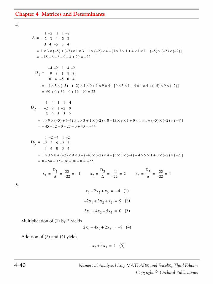
Chapter 4 Matrices and Determinants
4−40 Numerical Analysis Using MATLAB® and Excel®, Third EditionCopyright © Orchard Publications
4.
5. (1)
(2)
(3)
Multiplication of (1) by yields (4)
Addition of (2) and (4) yields
(5)
Δ1 2– 1 1 2–2– 3 1 2– 33 4 5– 3 4
=
1 3 5–( ) 2–( ) 1 3 1 2–( ) 4 3 3 1 4 1 1 5–( ) 2–( ) 2–( )××+××+××[ ]–××+××+××=
15– 6– 8– 9– 4– 20+ 22–==
D1
4– 2– 1 4 2–9 3 1 9 3
0 4 5– 0 4
=
4– 3 5–( ) 2–( ) 1 0 1 9 4 0 3 1 4 1 4 5–( ) 9 2–( )××+××+××[ ]–××+××+××=
60 0 36 0– 16 90–+ + + 22==
D2
1 4– 1 1 4–2– 9 1 2– 93 0 5– 3 0
=
1 9 5–( ) 4–( ) 1 3 1 2–( ) 0 3 9 1 0 1 1 5–( ) 2–( ) 4–( )××+××+××[ ]–××+××+××=
45– 12– 0– 27– 0– 40+ 44–==
D3
1 2– 4– 1 2–2– 3 9 2– 33 4 0 3 4
=
1 3 0 2–( ) 9 3 4–( ) 2–( ) 4 3 3 4–( ) 4 9 1 0 2–( ) 2–( )××+××+××[ ]–××+××+××=
0 54– 32 36 36– 0–+ + 22–==
x1
D1Δ
------- 2222–
--------- 1–= = = x2
D2Δ
------- 44–22–
--------- 2= = = x3
D3Δ
------- 22–22–
--------- 1= = =
x1 2x2 x3+– 4–=
2x– 1 3x2 x3+ + 9=
3x1 4x2 5x3–+ 0=
22x1 4x2 2x3+– 8–=
x2 3x3+– 1=
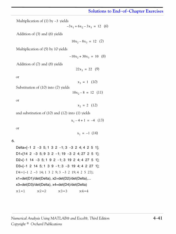
Numerical Analysis Using MATLAB® and Excel®, Third Edition 4−41Copyright © Orchard Publications
Solutions to End−of−Chapter Exercises
Multiplication of (1) by yields (6)
Addition of (3) and (6) yields
(7)
Multiplication of (5) by 10 yields
(8)
Addition of (7) and (8) yields (9)
or (10)
Substitution of (10) into (7) yields (11)
or (12)
and substitution of (10) and (12) into (1) yields
(13)
or (14)
6.
Delta=[−1 2 −3 5; 1 3 2 −1; 3 −3 2 4; 4 2 5 1];
D1=[14 2 −3 5; 9 3 2 −1; 19 −3 2 4; 27 2 5 1];
D2=[−1 14 −3 5; 1 9 2 −1; 3 19 2 4; 4 27 5 1];
D3=[−1 2 14 5; 1 3 9 −1; 3 −3 19 4; 4 2 27 1];
D4=[−1 2 −3 14; 1 3 2 9; 3 −3 2 19; 4 2 5 27];
x1=det(D1)/det(Delta), x2=det(D2)/det(Delta),...
x3=det(D3)/det(Delta), x4=det(D4)/det(Delta)
x1=1 x2=2 x3=3 x4=4
3–
3– x1 6x2 3x3–+ 12=
10x2 8x3– 12=
10x2 30x3+– 10=
22x3 22=
x3 1=
10x2 8– 12=
x2 2=
x1 4 1+– 4–=
x1 1–=
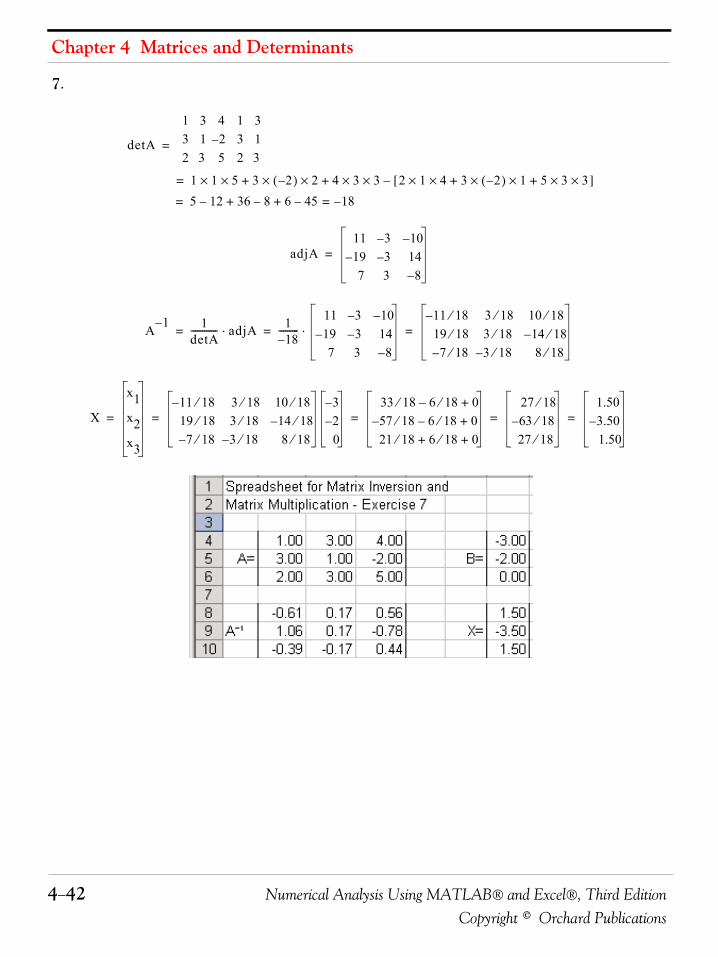
Chapter 4 Matrices and Determinants
4−42 Numerical Analysis Using MATLAB® and Excel®, Third EditionCopyright © Orchard Publications
7.
detA
1 3 43 1 2–2 3 5
1 33 12 3
1 1 5 3 2–( ) 2 4 3 3 2 1 4 3 2–( )×+×× 1 5 3 3××+×[ ]–××+××+××=
=
5 12– 36 8– 6 45–+ + 18–==
adjA11 3– 10–19– 3– 147 3 8–
=
A 1– 1detA------------ adjA⋅ 1
18–---------
11 3– 10–19– 3– 147 3 8–
⋅11 18⁄– 3 18⁄ 10 18⁄19 18⁄ 3 18⁄ 14 18⁄–7 18⁄– 3– 18⁄ 8 18⁄
= = =
X
x1x2x3
11 18⁄– 3 18⁄ 10 18⁄19 18⁄ 3 18⁄ 14 18⁄–7 18⁄– 3– 18⁄ 8 18⁄
3–2–0
33 18 6 18⁄– 0+⁄57– 18 6 18 0+⁄–⁄21 18 6 18⁄ 0+ +⁄
27 18⁄63– 18⁄27 18⁄
1.503.50–1.50
= = = = =
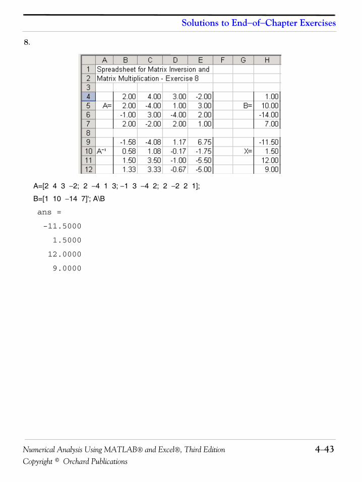
Numerical Analysis Using MATLAB® and Excel®, Third Edition 4−43Copyright © Orchard Publications
Solutions to End−of−Chapter Exercises
8.
A=[2 4 3 −2; 2 −4 1 3; −1 3 −4 2; 2 −2 2 1];
B=[1 10 −14 7]'; A\B
ans =
-11.5000
1.5000
12.0000
9.0000
Numerical Analysis Using MATLAB® and Excel®, Third Edition 5−1Copyright © Orchard Publications
Chapter 5
Differential Equations, State Variables, and State Equations
his chapter is a review of ordinary differential equations and an introduction to state vari-ables and state equations. Solutions of differential equations with numerical methods is dis-cussed in Chapter 9.
5.1 Simple Differential EquationsIn this section we present two simple examples to show the importance of differential equations inengineering applications.
Example 5.1 The current and voltage in a capacitor are related by
(5.1)
where is the current through the capacitor, is the voltage across the capacitor, and theconstant is the capacitance in farads (F). For this example and the capacitor is beingcharged by a constant current . Find the voltage across this capacitor as a function of timegiven that the voltage at some reference time is .
Solution:
It is given that the current, as a function of time, is constant, that is,
(5.2)
By substitution of (5.2) into (5.1) we obtain
and by separation of the variables,(5.3)
Integrating both sides of (5.3) we obtain(5.4)
where represents the constants of integration of both sides.
T
iC t( ) CdvCdt
---------=
iC t( ) vC t( )
C C 1 F=
I vC
t 0= V0
iC t( ) I cons ttan= =
dvCdt
--------- I=
dvC Idt=
vC t( ) It k+=
k
Chapter 5 Differential Equations, State Variables, and State Equations
5−2 Numerical Analysis Using MATLAB® and Excel®, Third EditionCopyright © Orchard Publications
We can find the value of the constant by making use of the initial condition, i.e., at , and (5.4) then becomes
(5.5)
or , and by substitution into (5.4),
(5.6)
This example shows that when a capacitor is charged with a constant current, a linear voltage is pro-duced across the terminals of the capacitor.
Example 5.2
Find the current through an inductor whose slope at the coordinate is and thecurrent passes through the point .
Solution:
We are given that
(5.7)
By separating the variables we obtain(5.8)
and integrating both sides we obtain(5.9)
where represents the constants of integration of both sides.
We find the value of the constant by making use of the initial condition. For this example, and thus at , . With these values (5.9) becomes
(5.10)
or , and by substitution into (5.9),
(5.11)
5.2 ClassificationDifferential equations are classified by:
1. Type - Ordinary or Partial
k t 0=
vC V0=
V0 0 k+=
k V0=
vC t( ) It V0+=
iL t( ) t iL,( ) tcos
iL π 2⁄ 1,( )
diLdt------- tcos=
diL tdtcos=
iL t( ) t k+sin=
k
kω 1= ωt t π 2⁄= = iL 1=
1 π2---sin k+=
k 0=
iL t( ) tsin=
Numerical Analysis Using MATLAB® and Excel®, Third Edition 5−3Copyright © Orchard Publications
Classification
2. Order - The highest order derivative which is included in the differential equation
3. Degree - The exponent of the highest power of the highest order derivative after the differentialequation has been cleared of any fractions or radicals in the dependent variable and its deriva-tives
For example, the differential equation
is an ordinary differential equation of order and degree .
If the dependent variable is a function of only a single variable , that is, if , the differ-ential equation which relates and is said to be an ordinary differential equation and it is abbrevi-ated as ODE.
The differential equation
is an ODE with constant coefficients.
The differential equation
is an ODE with variable coefficients.
If the dependent variable is a function of two or more variables such as , where and are independent variables, the differential equation that relates , , and is said to be apartial differential equation and it is abbreviated as PDE.
An example of a partial differential equation is the well-known one-dimensional wave equationshown below.
Most engineering problems are solved with ordinary differential equations with constant coeffi-cients; however, partial differential equations provide often quick solutions to some practicalapplications as illustrated with the following three examples.
d4ydx4--------⎝ ⎠⎜ ⎟⎛ ⎞ 2
5 d3ydx3--------⎝ ⎠⎜ ⎟⎛ ⎞ 4
6 d2ydx2--------⎝ ⎠⎜ ⎟⎛ ⎞ 6
3 dydx------⎝ ⎠⎛ ⎞ 8 y2
x3 1+--------------+ + + + ye 2x–=
4 2
y x y f x( )=
y x
d2ydt2-------- 3dy
dt------ 2+ + 5 4tcos=
x2 d2ydt2-------- xdy
dt------ x2 n2–( )+ + 0=
y y f x t,( )= xt y x t
∂2y∂t2-------- a2∂2y
∂x2--------=
Chapter 5 Differential Equations, State Variables, and State Equations
5−4 Numerical Analysis Using MATLAB® and Excel®, Third EditionCopyright © Orchard Publications
Example 5.3
The equivalent resistance of three resistors , , and in parallel is obtained from
Given that initially , , and , compute the change in if isincreased by and is decreased by while does not change.
Solution:
The initial value of the equivalent resistance is .
Now, we treat and as constants and differentiating with respect to we obtain
Similarly,
and the total differential is
By substitution of the given numerical values we obtain
Therefore, the eequivalent resistance decreases by .
Example 5.4
In a series electric circuit that is excited by a sinusoidal voltage, the magnitude of the imped-
ance is computed from . Initially, and . Find the changein the impedance if the resistance is increased by ( ) and the capacitive reac-tance is decreased by ( ).
RT R1 R2 R3
1RT------ 1
R1------ 1
R2------ 1
R3------+ +=
R1 5 Ω= R2 20 Ω= R3 4 Ω= RT R2
10 % R3 5 % R1
RT 5 20 4|| || 2 Ω= =
R2 R3 RT R1
1RT
2------–
∂RT∂R1---------- 1
R12
------–= or ∂RT∂R1----------
RTR1------⎝ ⎠
⎛ ⎞2
=
∂RT∂R2----------
RTR2------⎝ ⎠
⎛ ⎞2
= and ∂RT∂R3----------
RTR3------⎝ ⎠
⎛ ⎞2
=
dRT
RT∂RT∂R1----------dR1
∂RT∂R2----------dR2
∂RT∂R3----------dR3+ +
RTR1------⎝ ⎠
⎛ ⎞2dR1
RTR2------⎝ ⎠
⎛ ⎞2dR2
RTR3------⎝ ⎠
⎛ ⎞2dR+ += =
dRT25---⎝ ⎠
⎛ ⎞ 20( ) 2
20------⎝ ⎠
⎛ ⎞ 22( ) 2
4---⎝ ⎠
⎛ ⎞ 20.2–( )+ + 0.02 0.05– 0.03–= = =
3 %
RC
Z Z R 2 XC2+= R 4 Ω= XC 3 Ω=
Z R 0.25 Ω 6.25 %XC 0.125 Ω 4.167%–
Numerical Analysis Using MATLAB® and Excel®, Third Edition 5−5Copyright © Orchard Publications
Classification
Solution:
We will first find the partial derivatives and ; then we compute the change in impedance
from the total differential . Thus,
and
and by substitution of the given values
Therefore, if increases by and decreases by , the impedance increases by.
Example 5.5
A light bulb is rated at volts and watts. If the voltage decreases by volts and the resis-tance of the bulb is increased by , by how much will the power change?
Solution:
At volts and watts, the bulb resistance is
and since
and the total differential is
That is, the power will decrease by watts.
∂Z∂R------- ∂Z
∂XC----------
dZ
∂Z∂R------- R
R 2 XC2+
---------------------------= and ∂Z∂XC----------
XC
R 2 XC2+
---------------------------=
dZ ∂Z∂R------- dR ∂Z
∂XC---------- dXC+
R dR XC dXC+
R 2 XC2+
----------------------------------------= =
dZ 4 0.25( ) 3 0.125–( )+
4 2 32+----------------------------------------------------- 1 0.375 –
5-------------------------- 0.125= = =
R 6.25 % XC 4.167% Z
4.167%
120 75 58 Ω
V 120= P 75=
R V2
P------ 120 2
75------------ 192 Ω= = =
P V2
R------= then ∂P
∂V------- 2V
R-------= and ∂P
∂R------- V2
R2------–=
dP ∂P∂V------- dV ∂P
∂R------- dR+ 2V
R-------dV V2
R2------– dR 2 120( )
192----------------- 5–( ) 1202
1922-----------– 8( ) 9.375–= = ==
9.375
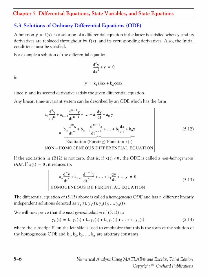
Chapter 5 Differential Equations, State Variables, and State Equations
5−6 Numerical Analysis Using MATLAB® and Excel®, Third EditionCopyright © Orchard Publications
5.3 Solutions of Ordinary Differential Equations (ODE)
A function is a solution of a differential equation if the latter is satisfied when and itsderivatives are replaced throughout by and its corresponding derivatives. Also, the initialconditions must be satisfied.
For example a solution of the differential equation
is
since and its second derivative satisfy the given differential equation.
Any linear, time-invariant system can be described by an ODE which has the form
(5.12)
If the excitation in (B12) is not zero, that is, if , the ODE is called a non-homogeneousODE. If , it reduces to:
(5.13)
The differential equation of (5.13) above is called a homogeneous ODE and has different linearlyindependent solutions denoted as .
We will now prove that the most general solution of (5.13) is:(5.14)
where the subscript on the left side is used to emphasize that this is the form of the solution ofthe homogeneous ODE and are arbitrary constants.
y f x( )= yf x( )
d2ydx2-------- y+ 0=
y k1 xsin k2 xcos+=
y
and nydtn--------- an 1–
d n 1– ydt n 1–---------------- … a1
dydt------ a0 y+ + + +
bm
d mxdt m---------- bm 1–
d m 1– xdt n 1–----------------- … b1
dxdt------ b0x+ + + +
Excitation Forcing( ) Function x t( )
=
NON HOMOGENEOUS DIFFERENTIAL EQUATION–
⎧ ⎪ ⎪ ⎪ ⎪ ⎪ ⎪ ⎪ ⎨ ⎪ ⎪ ⎪ ⎪ ⎪ ⎪ ⎪ ⎩
x t( ) 0≠x t( ) 0=
and nydtn--------- an 1–
d n 1– ydt n 1–---------------- … a1
dydt------ a0 y+ + + + 0=
HOMOGENEOUS DIFFERENTIAL EQUATION
ny1 t( ) y2 t( ) y3 t( ) … yn t( ), ,,,
yH t( ) k1 y1 t( ) k2 y2 t( ) k3 y3 t( ) … kn yn t( )+ + + +=
Hk1 k2 k3 … kn, , , ,
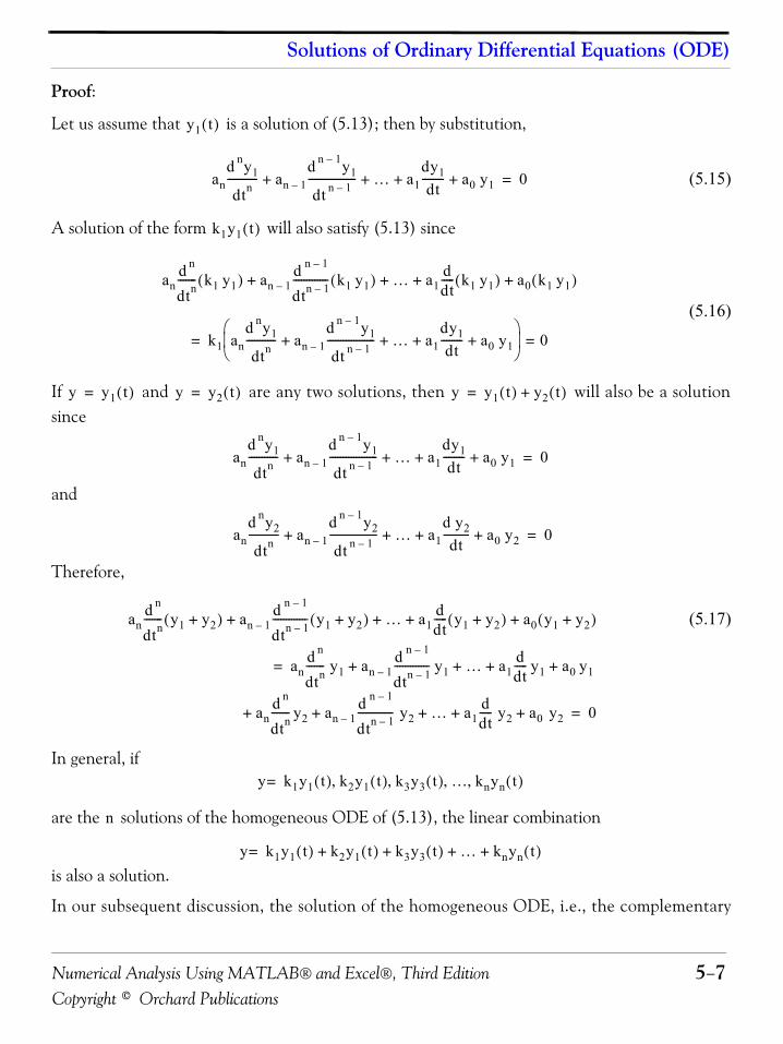
Numerical Analysis Using MATLAB® and Excel®, Third Edition 5−7Copyright © Orchard Publications
Solutions of Ordinary Differential Equations (ODE)
Proof:
Let us assume that is a solution of (5.13); then by substitution,
(5.15)
A solution of the form will also satisfy (5.13) since
(5.16)
If and are any two solutions, then will also be a solutionsince
and
Therefore,
(5.17)
In general, if
are the solutions of the homogeneous ODE of (5.13), the linear combination
is also a solution.
In our subsequent discussion, the solution of the homogeneous ODE, i.e., the complementary
y1 t( )
and ny1
dtn----------- an 1–
d n 1– y1
dt n 1–------------------ … a1
dy1dt
-------- a0 y1+ + + + 0=
k1y1 t( )
and n
dtn------- k1 y1( ) an 1–
d n 1–
dtn 1–------------- k1 y1( ) … a1
ddt----- k1 y1( ) a0 k1 y1( )+ + + +
k1 and ny1
dtn----------- an 1–
d n 1– y1
dt n 1–------------------ … a1
dy1dt
-------- a0 y1+ + + +⎝ ⎠⎜ ⎟⎛ ⎞
0==
y y1 t( )= y y2 t( )= y y1 t( ) y2 t( )+=
and ny1
dtn----------- an 1–
d n 1– y1
dt n 1–------------------ … a1
dy1dt
-------- a0 y1+ + + + 0=
and ny2
dtn----------- an 1–
d n 1– y2
dt n 1–------------------ … a1
d y2dt
---------- a0 y2+ + + + 0=
and n
dtn------- y1 y2+( ) an 1–
d n 1–
dtn 1–------------- y1 y2+( ) … a1
ddt----- y1 y2+( ) a0 y1 y2+( )+ + + +
and n
dtn------- y1 an 1–
d n 1–
dtn 1–------------- y1 … a1
ddt----- y1 a0 y1
and n
dtn------- y2 an 1–
d n 1–
dtn 1–------------- y2 … a1
ddt----- y2 a0 y2
+ + + +
+ + + + + 0
=
=
y k1y1 t( ) k2y1 t( ) k3y3 t( ) … knyn t( ), ,,,=
n
y k1y1 t( ) k2y1 t( ) k3y3 t( ) … knyn t( )+ +++=
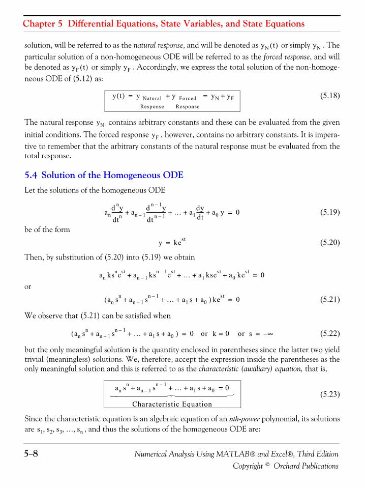
Chapter 5 Differential Equations, State Variables, and State Equations
5−8 Numerical Analysis Using MATLAB® and Excel®, Third EditionCopyright © Orchard Publications
solution, will be referred to as the natural response, and will be denoted as or simply . Theparticular solution of a non-homogeneous ODE will be referred to as the forced response, and willbe denoted as or simply . Accordingly, we express the total solution of the non-homoge-neous ODE of (5.12) as:
(5.18)
The natural response contains arbitrary constants and these can be evaluated from the giveninitial conditions. The forced response , however, contains no arbitrary constants. It is impera-tive to remember that the arbitrary constants of the natural response must be evaluated from thetotal response.
5.4 Solution of the Homogeneous ODELet the solutions of the homogeneous ODE
(5.19)
be of the form
(5.20)
Then, by substitution of (5.20) into (5.19) we obtain
or
(5.21)
We observe that (5.21) can be satisfied when
(5.22)
but the only meaningful solution is the quantity enclosed in parentheses since the latter two yieldtrivial (meaningless) solutions. We, therefore, accept the expression inside the parentheses as theonly meaningful solution and this is referred to as the characteristic (auxiliary) equation, that is,
(5.23)
Since the characteristic equation is an algebraic equation of an nth-power polynomial, its solutionsare , and thus the solutions of the homogeneous ODE are:
yN t( ) yN
yF t( ) yF
y t( ) y NaturalResponse
y ForcedResponse
+ yN yF+= =
yN
yF
and nydtn--------- an 1–
d n 1– ydt n 1–---------------- … a1
dydt------ a0 y+ + + + 0=
y kest=
an ksnest an 1– ksn 1– est … a1 ksest a0 kest+ + + + 0=
an sn an 1– sn 1– … a1 s a0+ + + +( ) kest 0=
an sn an 1– sn 1– … a1 s a0+ + + +( ) 0 or k 0 or s= ∞–= =
an sn an 1– sn 1– … a1 s a0+ + + + 0=
Characteristic Equation
⎧ ⎪ ⎪ ⎪ ⎪ ⎪ ⎪ ⎪ ⎨ ⎪ ⎪ ⎪ ⎪ ⎪ ⎪ ⎪ ⎩
s1 s2 s3 … sn, , , ,
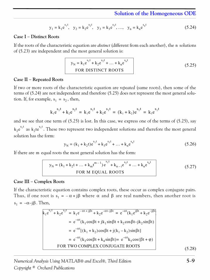
Numerical Analysis Using MATLAB® and Excel®, Third Edition 5−9Copyright © Orchard Publications
Solution of the Homogeneous ODE
(5.24)
Case I − Distinct Roots
If the roots of the characteristic equation are distinct (different from each another), the solutionsof (5.23) are independent and the most general solution is:
(5.25)
Case II − Repeated Roots
If two or more roots of the characteristic equation are repeated (same roots), then some of theterms of (5.24) are not independent and therefore (5.25) does not represent the most general solu-tion. If, for example, , then,
and we see that one term of (5.25) is lost. In this case, we express one of the terms of (5.25), say
as . These two represent two independent solutions and therefore the most generalsolution has the form:
(5.26)
If there are equal roots the most general solution has the form:
(5.27)
Case III − Complex Roots
If the characteristic equation contains complex roots, these occur as complex conjugate pairs.Thus, if one root is where and are real numbers, then another root is
. Then,
(5.28)
y1 k1es1t
= y2 k2es2t
= y3 k3es3t
= … yn knesnt
=, , , ,
n
yN k1es1t
= k2es2t
… knesnt
+ + +
FOR DISTINCT ROOTS
s1 s2=
k1es1t
k2es2t
+ k1es1t
k2es1t
+ k1 k2+( )es1t
k3es1t
= = =
k2es1t
k2tes1t
yN k1 k2t+( )es1t
= k3es3t
… knesnt
+ + +
m
yN k1 k2t … kmtm 1–+ + +( ) es1t
= kn i– es2t
… knesnt
+ + +
FOR M EQUAL ROOTS
s1 α– jβ+= α β
s1 α– j– β=
k1es1t
k2es2t
+ k1e αt– jβ t+ k2e αt– j– β t+ e αt– k1ejβt k2e j– β t+( )= =
e αt– k1 βtcos jk1 βsin t k2 βtcos jk2– βsin t+ +( )=
e αt– k1 k2+( ) βtcos j k1 k2–( ) βsin t+[ ]=
e αt– k3 βtcos k4 βsin t+( ) e αt– k5 βt ϕ+( )cos==
FOR TWO COMPLEX CONJUGATE ROOTS
Chapter 5 Differential Equations, State Variables, and State Equations
5−10 Numerical Analysis Using MATLAB® and Excel®, Third EditionCopyright © Orchard Publications
If (5.28) is to be a real function of time, the constants and must be complex conjugates.The other constants , , , and the phase angle are real constants.
The forced response can be found by
a. The Method of Undetermined Coefficients or
b. The Method of Variation of Parameters
We will study the Method of Undetermined Coefficients first.
5.5 Using the Method of Undetermined Coefficients for the Forced Response
For simplicity, we will only consider ODEs of . Higher order ODEs are discussed in differ-ential equations textbooks.
Consider the non-homogeneous ODE
(5.29)
where , , and are real constants.
We have learned that the total (complete) solution consists of the summation of the natural andforced responses.
For the natural response, if and are any two solutions of (5.29), the linear combination, where and are arbitrary constants, is also a solution, that is, if we know
the two solutions, we can obtain the most general solution by forming the linear combination of and . To be certain that there exist no other solutions, we examine the Wronskian Determi-
nant defined below.
(5.30)
If (5.30) is true, we can be assured that all solutions of (5.29) are indeed the linear combination of and .
The forced response is obtained by observation of the right side of the given ODE as it is illus-trated by the examples that follow.
k1 k2
k3 k4 k5 ϕ
order 2
at2
2
d
d y b ddt-----y cy+ + f x( )=
a b c
y1 y2
y3 k1 y1 k2 y2+= k1 k2
y1 y2
W y1 y2,( )y1 y2
ddx------ y1
ddx------ y2
≡ y1d
dx------ y2 y2
ddx------ y1– 0≠=
WRONSKIAN DETERMINANT
y1 y2
Numerical Analysis Using MATLAB® and Excel®, Third Edition 5−11Copyright © Orchard Publications
Using the Method of Undetermined Coefficients for the Forced Response
Example 5.6 Find the total solution of the ODE
(5.31)
subject to the initial conditions and where
Solution:
This is a homogeneous ODE and its total solution is just the natural response found from the char-
acteristic equation whose roots are and . The total response is:
(5.32)
The constants and are evaluated from the given initial conditions. For this example,
or(5.33)
Also,
or(5.34)
Simultaneous solution of (5.33) and (5.34) yields and . By substitution into(5.32), we obtain
(5.35)Check with MATLAB:
y=dsolve('D2y+4*Dy+3*y=0', 'y(0)=3', 'Dy(0)=4')
y =(-7/2*exp(-3*t)*exp(t)+13/2)/exp(t)
pretty(y) - 7/2 exp(-3 t) exp(t) + 13/2 ----------------------------- exp(t)
The function , of relation (5.35), shown in Figure 5.1, was plotted with the use of theMATLAB script
t2
2
d
d y 4dydt------ 3y+ + 0=
y 0( ) 3= y' 0( ) 4= y' dy dt⁄=
s2 4s 3+ + 0= s1 1–= s2 3–=
y t( ) yN t( ) k1e t– k2e 3t–+= =
k1 k2
y 0( ) 3 k1e0 k2e0 += =
k1 k2+ 3=
y' 0( ) 4 dydt------
t 0=
k1e t–– 3k2e 3t––t 0=
= = =
k1– 3k2– 4=
k1 6.5= k2 3.5–=
y t( ) yN t( ) 6.5e t– 3.5e 3t––= =
y f t( )=
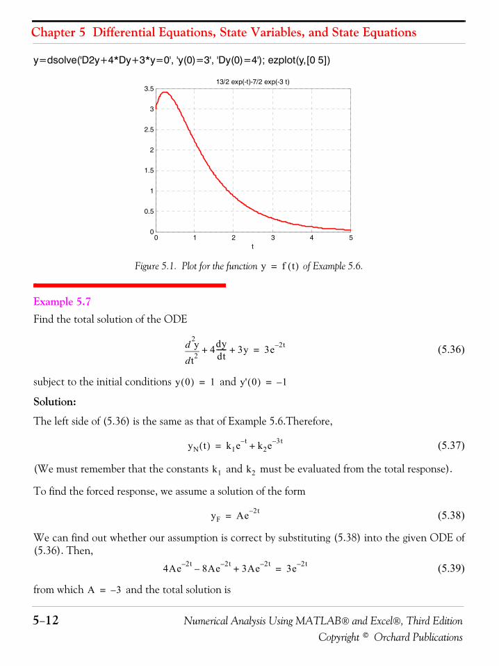
Chapter 5 Differential Equations, State Variables, and State Equations
5−12 Numerical Analysis Using MATLAB® and Excel®, Third EditionCopyright © Orchard Publications
y=dsolve('D2y+4*Dy+3*y=0', 'y(0)=3', 'Dy(0)=4'); ezplot(y,[0 5])
Figure 5.1. Plot for the function of Example 5.6.
Example 5.7 Find the total solution of the ODE
(5.36)
subject to the initial conditions and
Solution:
The left side of (5.36) is the same as that of Example 5.6.Therefore,
(5.37)
(We must remember that the constants and must be evaluated from the total response).
To find the forced response, we assume a solution of the form
(5.38)
We can find out whether our assumption is correct by substituting (5.38) into the given ODE of(5.36). Then,
(5.39)
from which and the total solution is
0 1 2 3 4 50
0.5
1
1.5
2
2.5
3
3.5
t
13/2 exp(-t)-7/2 exp(-3 t)
y f t( )=
t2
2
d
d y 4dydt------ 3y+ + 3e 2t–=
y 0( ) 1= y' 0( ) 1–=
yN t( ) k1e t– k2e 3t–+=
k1 k2
yF Ae 2t–=
4Ae 2t– 8Ae 2t–– 3Ae 2t–+ 3e 2t–=
A 3–=
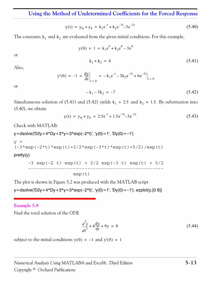
Numerical Analysis Using MATLAB® and Excel®, Third Edition 5−13Copyright © Orchard Publications
Using the Method of Undetermined Coefficients for the Forced Response
(5.40)
The constants and are evaluated from the given initial conditions. For this example,
or(5.41)
Also,
or (5.42)
Simultaneous solution of (5.41) and (5.42) yields and . By substitution into(5.40), we obtain
(5.43)
Check with MATLAB:
y=dsolve('D2y+4*Dy+3*y=3*exp(−2*t)', 'y(0)=1', 'Dy(0)=−1')
y = (-3*exp(-2*t)*exp(t)+3/2*exp(-3*t)*exp(t)+5/2)/exp(t)
pretty(y)
-3 exp(-2 t) exp(t) + 3/2 exp(-3 t) exp(t) + 5/2 ------------------------------------------------ exp(t)
The plot is shown in Figure 5.2 was produced with the MATLAB script
y=dsolve('D2y+4*Dy+3*y=3*exp(−2*t)', 'y(0)=1', 'Dy(0)=−1'); ezplot(y,[0 8])
Example 5.8 Find the total solution of the ODE
(5.44)
subject to the initial conditions and
y t( ) yN yF+ k1e t– k2e 3t– 3– e 2t–+= =
k1 k2
y 0( ) 1 k1e0 k2e0 3e0–+= =
k1 k2+ 4=
y' 0( ) 1– dydt------
t 0=
k1e t–– 3k2e 3t–– 6e 2t–+t 0=
= = =
k1– 3k2– 7–=
k1 2.5= k2 1.5=
y t( ) yN yF+ 2.5e t– 1.5e 3t– 3– e 2t–+= =
t2
2
d
d y 6dydt------ 9y+ + 0=
y 0( ) 1–= y' 0( ) 1=
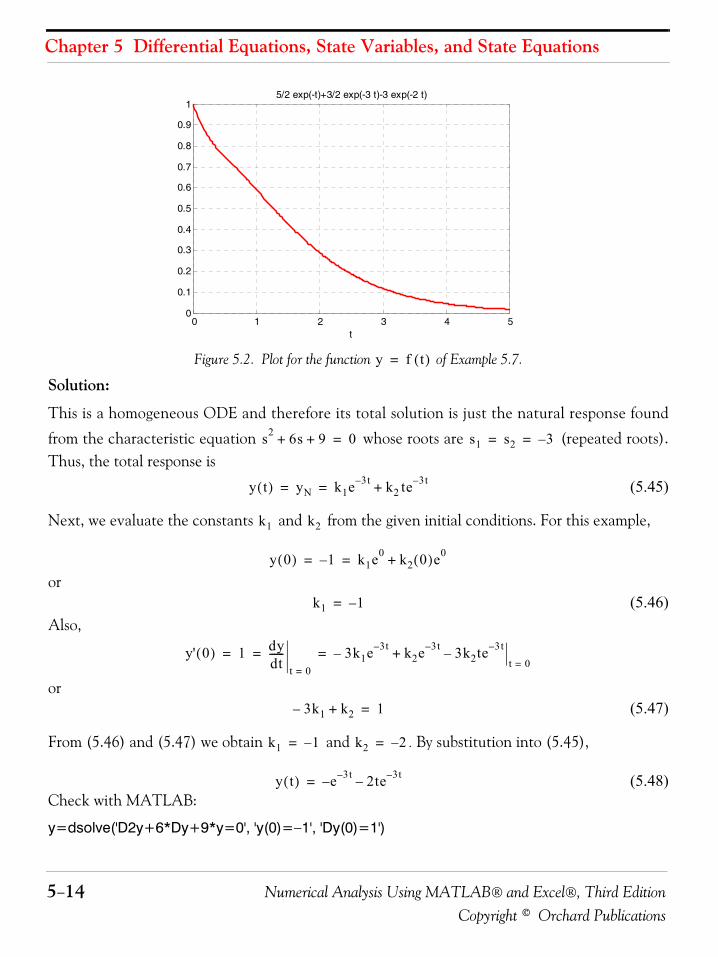
Chapter 5 Differential Equations, State Variables, and State Equations
5−14 Numerical Analysis Using MATLAB® and Excel®, Third EditionCopyright © Orchard Publications
Figure 5.2. Plot for the function of Example 5.7.
Solution:
This is a homogeneous ODE and therefore its total solution is just the natural response found
from the characteristic equation whose roots are (repeated roots).Thus, the total response is
(5.45)
Next, we evaluate the constants and from the given initial conditions. For this example,
or
(5.46)Also,
or(5.47)
From (5.46) and (5.47) we obtain and . By substitution into (5.45),
(5.48)Check with MATLAB:
y=dsolve('D2y+6*Dy+9*y=0', 'y(0)=−1', 'Dy(0)=1')
0 1 2 3 4 50
0.1
0.2
0.3
0.4
0.5
0.6
0.7
0.8
0.9
1
t
5/2 exp(-t)+3/2 exp(-3 t)-3 exp(-2 t)
y f t( )=
s2 6s 9+ + 0= s1 s2 3–= =
y t( ) yN k1e 3t– k2 te 3t–+= =
k1 k2
y 0( ) 1– k1e0 k2 0( )e0+= =
k1 1–=
y' 0( ) 1 dydt------
t 0=
3k1e 3t–– k2e 3t– 3k2te 3t––+t 0=
= = =
3k1– k2+ 1=
k1 1–= k2 2–=
y t( ) e– 3t– 2te 3t––=
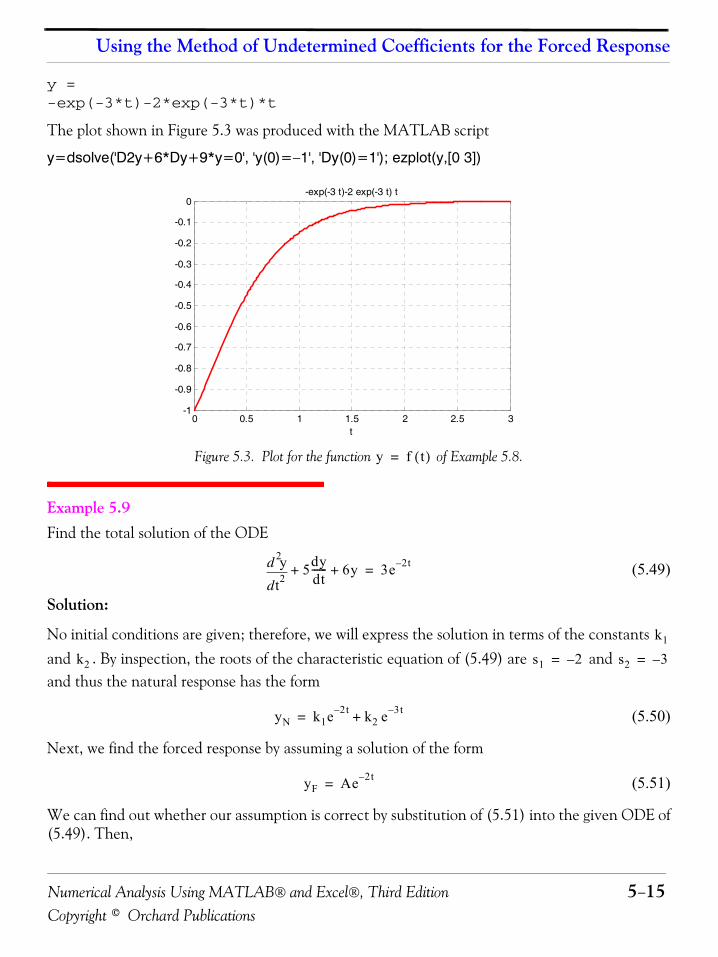
Numerical Analysis Using MATLAB® and Excel®, Third Edition 5−15Copyright © Orchard Publications
Using the Method of Undetermined Coefficients for the Forced Response
y =-exp(-3*t)-2*exp(-3*t)*t
The plot shown in Figure 5.3 was produced with the MATLAB script
y=dsolve('D2y+6*Dy+9*y=0', 'y(0)=−1', 'Dy(0)=1'); ezplot(y,[0 3])
Figure 5.3. Plot for the function of Example 5.8.
Example 5.9 Find the total solution of the ODE
(5.49)
Solution:
No initial conditions are given; therefore, we will express the solution in terms of the constants and . By inspection, the roots of the characteristic equation of (5.49) are and and thus the natural response has the form
(5.50)
Next, we find the forced response by assuming a solution of the form
(5.51)
We can find out whether our assumption is correct by substitution of (5.51) into the given ODE of(5.49). Then,
0 0.5 1 1.5 2 2.5 3-1
-0.9
-0.8
-0.7
-0.6
-0.5
-0.4
-0.3
-0.2
-0.1
0
t
-exp(-3 t)-2 exp(-3 t) t
y f t( )=
t2
2
d
d y 5dydt------ 6y+ + 3e 2t–=
k1
k2 s1 2–= s2 3–=
yN k1e 2t– k2 e 3t–+=
yF Ae 2t–=
Chapter 5 Differential Equations, State Variables, and State Equations
5−16 Numerical Analysis Using MATLAB® and Excel®, Third EditionCopyright © Orchard Publications
(5.52)
but the sum of the three terms on the left side of (5.52) is zero whereas the right side can never bezero unless we let and this produces a meaningless result.
The problem here is that the right side of the given ODE of (5.49) has the same form as one of the
terms of the natural response of (5.50), namely the term .
To work around this problem, we assume that the forced response has the form
(5.53)
that is, we multiply (5.51) by in order to eliminate the duplication of terms in the total response.Then, by substitution of (5.53) into (5.49) and equating like terms, we find that . There-fore, the total response is
(5.54)
Check with MATLAB:
y=dsolve('D2y+5*Dy+6*y=3*exp(−2*t)')
y =-3*exp(-2*t)+3*t*exp(-2*t)+C1*exp(-3*t)+C2*exp(-2*t)
We observe that the first and last terms of the displayed expression above have the same form andthus they can be combined to form a single term C3*exp(-2*t).
Example 5.10 Find the total solution of the ODE
(5.55)
Solution:
No initial conditions are given; therefore, we will express solution in terms of the constants and . We observe that the left side of (5.55) is the same of that of Example 5.9. Therefore, thenatural response is the same, that is, it has the form
(5.56)
Next, to find the forced response and we assume a solution of the form
4Ae 2t– 10Ae 2t–– 6Ae 2t–+ 3e 2t–=
t ∞→
k1 e 2t–
yF Ate 2t–=
tA 3=
y t( ) yN yF+ k1e 2t– k2e 3t– 3te 2t–+ += =
t2
2
d
d y 5dydt------ 6y+ + 4 5tcos=
k1
k2
yN k1e 2t– k2e 3t–+=
Numerical Analysis Using MATLAB® and Excel®, Third Edition 5−17Copyright © Orchard Publications
Using the Method of Undetermined Coefficients for the Forced Response
(5.57)
We can find out whether our assumption is correct by substitution of the assumed solution of(5.57) into the given ODE of (5.56). Then,
but this relation is invalid since by equating cosine and sine terms, we find that andalso . This inconsistency is a result of our failure to recognize that the derivatives of produce new terms of the form and these terms must be included in the forced response.Accordingly, we let
(5.58)
and by substitution into (5.55) we obtain
Collecting like terms and equating sine and cosine terms, we obtain the following set of equations
(5.59)
We use MATLAB to solve (5.59)
format rat; [k3 k4]=solve(19*x+25*y, 25*x−19*y−4)
k3 =50/493k4 =-38/493
Therefore, the total solution is
(5.60)
Check with MATLAB:
y=dsolve('D2y+5*Dy+6*y=4*cos(5*t)'); y=simple(y)
y =-38/493*cos(5*t)+50/493*sin(5*t)+C1*exp(-3*t)+C2*exp(-2*t)
In most engineering problems the right side of the non−homogeneous ODE consists of elementary
functions such as (constant), where is a positive integer, , , , and linearcombinations of these. Table 5.1 summarizes the forms of the forced response for a second order
yF A 5tcos=
25A 5tcos– 25A 5sin t– 6A 5tcos+ 19A 5tcos– 25A 5sin t– 4 5tcos= =
A 4– 19⁄=
A 0= A 5tcosB 5tsin
yF k3 5sin t k4 5tcos+=
25– k3 5tsin 25k4 5cos t 25k3 5cos t+– 25k4 5sin t– 6k3 5tsin 6k4 5cos t+ + 4 5cos t=
19k3 25k4+ 0=
25k3 19– k4 4=
y t( ) yN yF t( )+ k1e 2t– k2e 3t– 50493--------- 5tsin 38–
493--------- 5tcos+ + += =
k xn n ekx kxcos kxsin
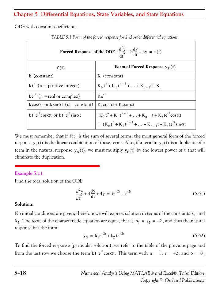
Chapter 5 Differential Equations, State Variables, and State Equations
5−18 Numerical Analysis Using MATLAB® and Excel®, Third EditionCopyright © Orchard Publications
ODE with constant coefficients.
We must remember that if is the sum of several terms, the most general form of the forcedresponse is the linear combination of these terms. Also, if a term in is a duplicate of aterm in the natural response , we must multiply by the lowest power of that willeliminate the duplication.
Example 5.11 Find the total solution of the ODE
(5.61)
Solution:
No initial conditions are given; therefore we will express solution in terms of the constants and. The roots of the characteristic equation are equal, that is, , and thus the natural
response has the form
(5.62)
To find the forced response (particular solution), we refer to the table of the previous page and
from the last row we choose the term . This term with , , and ,
TABLE 5.1 Form of the forced response for 2nd order differential equations
Forced Response of the ODE
Form of Forced Response
(constant) (constant)
( = positive integer)
( =real or complex)
or ( =constant)
or
+
ad2ydt2-------- bdy
dt------ cy+ + f t( )=
f t( ) yF t( )
k K
k t n n K0 t n K1 tn 1– … Kn 1– t Kn+ + + +
ker t r Ker t
k αtcos k αtsin α K1cosαt K2 αtsin+
k t ner t αtcos k t ner t αsin t K0 t n K1 tn 1– … Kn 1– t Kn+ + + +( )er t αtcos
K0 t n K1 tn 1– … Kn 1– t Kn+ + + +( )er t αtsin
f t( )yF t( ) yF t( )
yN t( ) yF t( ) t
t2
2
d
d y 4dydt------ 4y+ + te 2t– e 2t––=
k1
k2 s1 s2 2–= =
yN k1e 2– t k2 te 2– t+=
k t ner t αtcos n 1= r 2–= α 0=
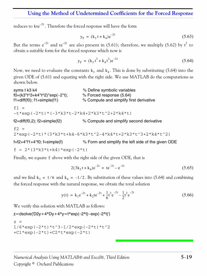
Numerical Analysis Using MATLAB® and Excel®, Third Edition 5−19Copyright © Orchard Publications
Using the Method of Undetermined Coefficients for the Forced Response
reduces to . Therefore the forced response will have the form
(5.63)
But the terms and are also present in (5.61); therefore, we multiply (5.62) by toobtain a suitable form for the forced response which now is
(5.64)
Now, we need to evaluate the constants and . This is done by substituting (5.64) into thegiven ODE of (5.61) and equating with the right side. We use MATLAB do the computations asshown below.
syms t k3 k4 % Define symbolic variablesf0=(k3*t^3+k4*t^2)*exp(−2*t); % Forced response (5.64)f1=diff(f0); f1=simple(f1) % Compute and simplify first derivative
f1 =-t*exp(-2*t)*(-3*k3*t-2*k4+2*k3*t^2+2*k4*t)
f2=diff(f0,2); f2=simple(f2) % Compute and simplify second derivative
f2 =2*exp(-2*t)*(3*k3*t+k4-6*k3*t^2-4*k4*t+2*k3*t^3+2*k4*t^2)
f=f2+4*f1+4*f0; f=simple(f) % Form and simplify the left side of the given ODE
f = 2*(3*k3*t+k4)*exp(-2*t)
Finally, we equate f above with the right side of the given ODE, that is
(5.65)
and we find and . By substitution of these values into (5.64) and combiningthe forced response with the natural response, we obtain the total solution
(5.66)
We verify this solution with MATLAB as follows:
z=dsolve('D2y+4*Dy+4*y=t*exp(−2*t)−exp(−2*t)')
z =1/6*exp(-2*t)*t^3-1/2*exp(-2*t)*t^2+C1*exp(-2*t)+C2*t*exp(-2*t)
kte 2– t
yF k3 t k4+( )e 2– t=
e 2t– te 2t– t2
yF k3 t3 k4 t2+( )e 2– t=
k3 k4
2 3k3 t k4+( )e 2t– te 2t– e 2t––=
k3 1 6⁄= k4 1 2⁄–=
y t( ) k1e 2– t k2te 2– t 16---t3e
2– t 12---t2e
2– t–+ +=
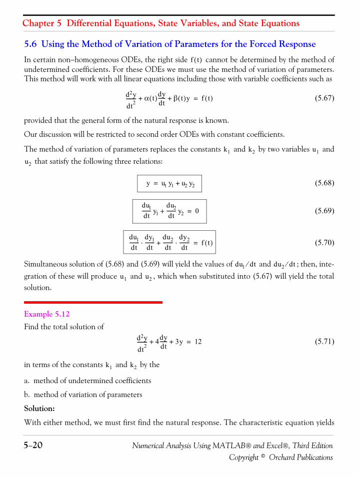
Chapter 5 Differential Equations, State Variables, and State Equations
5−20 Numerical Analysis Using MATLAB® and Excel®, Third EditionCopyright © Orchard Publications
5.6 Using the Method of Variation of Parameters for the Forced Response
In certain non−homogeneous ODEs, the right side cannot be determined by the method ofundetermined coefficients. For these ODEs we must use the method of variation of parameters.This method will work with all linear equations including those with variable coefficients such as
(5.67)
provided that the general form of the natural response is known.
Our discussion will be restricted to second order ODEs with constant coefficients.
The method of variation of parameters replaces the constants and by two variables and that satisfy the following three relations:
(5.68)
(5.69)
(5.70)
Simultaneous solution of (5.68) and (5.69) will yield the values of and ; then, inte-gration of these will produce and , which when substituted into (5.67) will yield the totalsolution.
Example 5.12 Find the total solution of
(5.71)
in terms of the constants and by the
a. method of undetermined coefficients
b. method of variation of parameters
Solution:
With either method, we must first find the natural response. The characteristic equation yields
f t( )
d2ydt2-------- α t( )dy
dt------ β t( )y+ + f t( )=
k1 k2 u1
u2
y u1 y1 u2 y2+=
du1dt------- y1
du2dt
-------- y2+ 0=
du1dt
--------dy1dt
--------⋅du2dt
--------dy2dt
--------⋅+ f t( )=
du1 dt⁄ du2 dt⁄
u1 u2
d2ydt2-------- 4dy
dt------ 3y+ + 12=
k1 k2
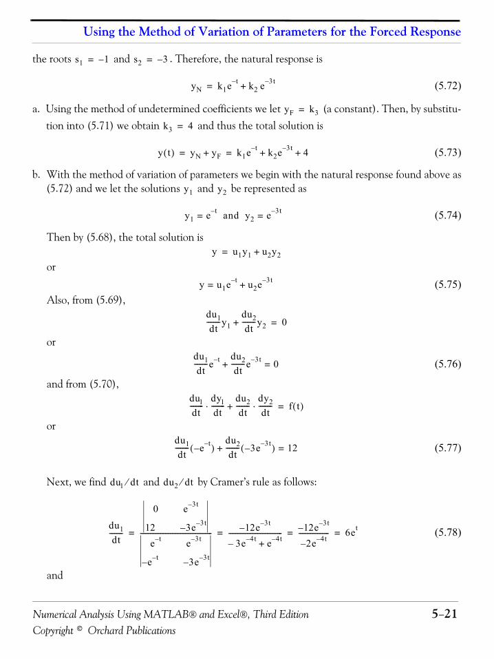
Numerical Analysis Using MATLAB® and Excel®, Third Edition 5−21Copyright © Orchard Publications
Using the Method of Variation of Parameters for the Forced Response
the roots and . Therefore, the natural response is
(5.72)
a. Using the method of undetermined coefficients we let (a constant). Then, by substitu-tion into (5.71) we obtain and thus the total solution is
(5.73)
b. With the method of variation of parameters we begin with the natural response found above as(5.72) and we let the solutions and be represented as
(5.74)
Then by (5.68), the total solution is
or
(5.75)Also, from (5.69),
or
(5.76)
and from (5.70),
or
(5.77)
Next, we find and by Cramer’s rule as follows:
(5.78)
and
s1 1–= s2 3–=
yN k1e t– k2 e 3– t+=
yF k3=
k3 4=
y t( ) yN yF+ k1e t– k2e 3– t 4+ += =
y1 y2
y1 e t–= and y2 e 3t–=
y u1y1 u2y2+=
y u1e t– u2e 3t–+=
du1dt
--------y1du2dt
--------y2+ 0=
du1dt
--------e t– du2dt
--------e 3t–+ 0=
du1dt
--------dy1dt
--------⋅du2dt
--------dy2dt
--------⋅+ f t( )=
du1dt
-------- e t––( )du2dt
-------- 3e 3t––( )+ 12=
du1 dt⁄ du2 dt⁄
du1dt
--------
0 e 3t–
12 3e 3t––
e t– e 3t–
e t–– 3e 3t––
------------------------------------------- 12e 3t––
3e 4t–– e 4t–+-------------------------------- 12e 3t––
2e 4t––------------------ 6et= = = =
Chapter 5 Differential Equations, State Variables, and State Equations
5−22 Numerical Analysis Using MATLAB® and Excel®, Third EditionCopyright © Orchard Publications
(5.79)
Now, integration of (5.78) and (5.79) and substitution into (5.75) yields
(5.80)
(5.81)
We observe that the last expression in (5.81) is the same as (5.73) of part (a).
Check with MATLAB:
y=dsolve('D2y+4*Dy+3*y=12')
y =(4*exp(t)+C1*exp(-3*t)*exp(t)+C2)/exp(t)
Example 5.13 Find the total solution of
(5.82)
in terms of the constants and by any method.
Solution:
This ODE cannot be solved by the method of undetermined coefficients; therefore, we will usethe method of variation of parameters.
The characteristic equation is from which and thus the natural response is
(5.83)We let
(5.84)Then, by (5.68) the solution is
(5.85)
du2dt
--------
e t– 0
e t–– 122e 4t––
--------------------------------- 12e t–
2e 4t––--------------- 6– e3t= = =
u1 6 et td∫ 6et k1+= = u2 6– e3t td∫ 2– e3t k2+= =
y u1e t– u2e 3t–+ 6et k1+( )e t– 2– e3t k2+( )e 3t–+= =
6 k1e t– 2 k2e 3t–+–+ k1e t– k2e 3t– 4+ +==
d2ydt2-------- 4y+ 2ttan=
k1 k2
s2 4+ 0= s j2±=
yN k1ej2t k2e j– 2t+=
y1 2tcos= and y2 2tsin=
y u1y1 u2y2 + u1 2tcos u2 2tsin += =
Numerical Analysis Using MATLAB® and Excel®, Third Edition 5−23Copyright © Orchard Publications
Using the Method of Variation of Parameters for the Forced Response
Also, from (5.69),
or
(5.86)
and from (5.70),
(5.87)
Next, we find and by Cramer’s rule as follows:
(5.88)
and
(5.89)
Now, integration of (5.88) and (5.89) and substitution into (5.85) yields
(5.90)
(5.91)
(5.92)
Check with MATLAB:
y=dsolve('D2y+4*y=tan(2*t)')
y =-1/4*cos(2*t)*log((1+sin(2*t))/cos(2*t))+C1*cos(2*t)+C2*sin(2*t)
du1dt
--------y1du2dt
--------y2+ 0=
du1dt
-------- 2tcosdu2dt
-------- 2tsin+ 0=
du1dt
--------dy1dt
--------⋅du2dt
--------dy2dt
--------⋅+ f t( )du1dt
--------= = 2 2tsin–( )du2dt
-------- 2 2tcos( )+ 2ttan=
du1 dt⁄ du2 dt⁄
du1dt
--------
0 2tsin2ttan 2 2tcos2tcos 2tsin
2 2tsin– 2 2tcos
------------------------------------------------------
2t2sin2tcos
---------------–
2 2t2cos 2 2t2sin+-------------------------------------------- 2t2sin–
2 2tcos------------------= = =
du2dt
--------
2tcos 02 2tsin– 2ttan
2-------------------------------------------------- 2tsin
2------------= =
u112---–
2t2sin2tcos
--------------- td∫ 2tsin4
------------ 14--- 2tsec 2ttan+( )ln– k1+= =
u212--- 2tsin td∫ 2tcos
4-------------– k2+= =
y u1y1 u2y2 + 2t 2tcossin4
--------------------------- 14--- 2t 2tsec 2ttan+( )lncos– k1 2tcos+ 2t 2tcossin
4---------------------------– k2 2tsin+= =
14--- 2t 2tsec 2ttan+( )lncos– k1 2tcos k2 2tsin+ +=
Chapter 5 Differential Equations, State Variables, and State Equations
5−24 Numerical Analysis Using MATLAB® and Excel®, Third EditionCopyright © Orchard Publications
5.7 Expressing Differential Equations in State Equation FormA first order differential equation with constant coefficients has the form
(5.93)
In a second order differential equation the highest order is a second derivative.
An nth−order differential equation can be resolved to first−order simultaneous differential equa-tions with a set of auxiliary variables called state variables. The resulting first−order differentialequations are called state space equations, or simply state equations. The state variable method offersthe advantage that it can also be used with non−linear and time−varying systems. However, ourdiscussion will be limited to linear, time−invariant systems.
State equations can also be solved with numerical methods such as Taylor series and Runge−Kutta methods; these will be discussed in Chapter 9. The state variable method is best illustratedthrough several examples presented in this chapter.
Example 5.14 A system is described by the integro−differential equation
(5.94)
Differentiating both sides and dividing by we obtain
(5.95)
or
(5.96)
Next, we define two state variables and such that
(5.97)and
(5.98)
Then,
(5.99)
a1dydt------ a0 y t( )+ x t( )=
n
Ri Ldidt----- 1
C---- i td
∞–
t
∫+ + e jωt=
L
d2tdt2------- R
L---- di
dt----- 1
LC-------- i+ + 1
L---jωe jωt=
d2tdt2------- R
L---- di
dt----- 1
LC-------- i 1
L---jωe jωt+––=
x1 x2
x1 i=
x2didt----- dx1
dt-------- x· 1= = =
x· 2 d2i dt2⁄=
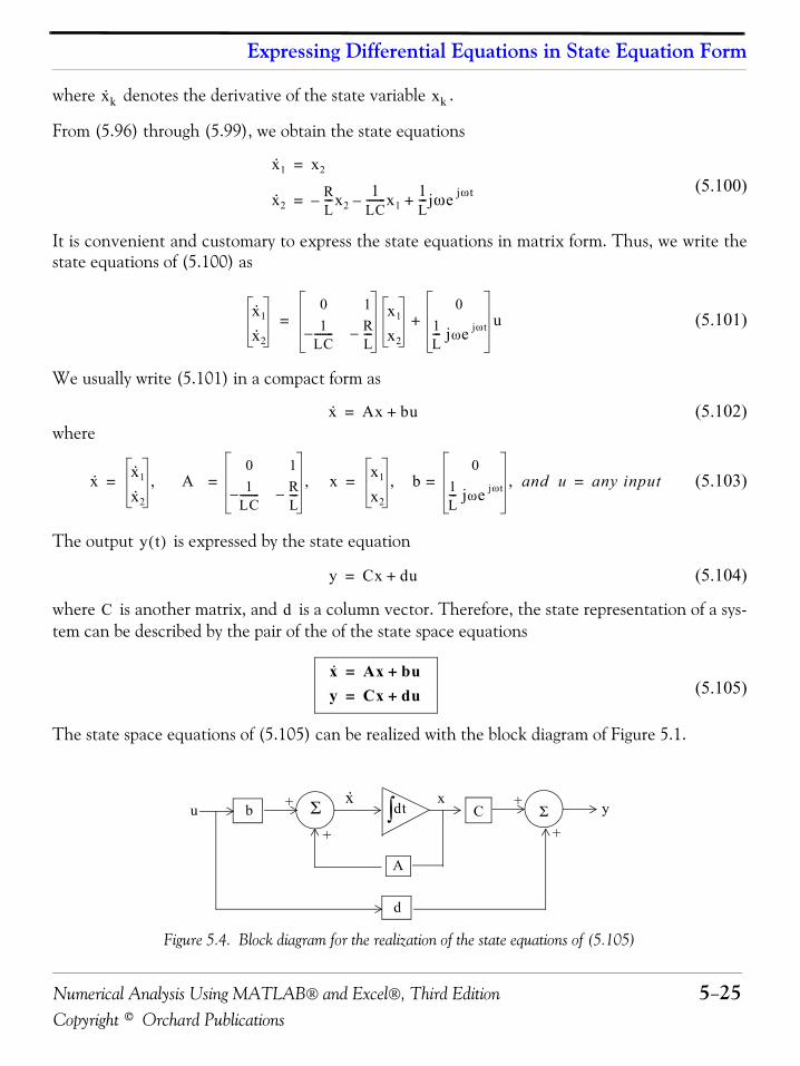
Numerical Analysis Using MATLAB® and Excel®, Third Edition 5−25Copyright © Orchard Publications
Expressing Differential Equations in State Equation Form
where denotes the derivative of the state variable .
From (5.96) through (5.99), we obtain the state equations
(5.100)
It is convenient and customary to express the state equations in matrix form. Thus, we write thestate equations of (5.100) as
(5.101)
We usually write (5.101) in a compact form as
(5.102)where
(5.103)
The output is expressed by the state equation
(5.104)
where is another matrix, and is a column vector. Therefore, the state representation of a sys-tem can be described by the pair of the of the state space equations
(5.105)
The state space equations of (5.105) can be realized with the block diagram of Figure 5.1.
Figure 5.4. Block diagram for the realization of the state equations of (5.105)
x· k xk
x· 1 x2=
x· 2RL---x2– 1
LC-------x1– 1
L---jωe jωt+=
x· 1
x· 2
0 11
LC-------– R
L---–
x1
x2
01L--- jωe jωt u+=
x· Ax bu+=
x· x· 1
x· 2
A 0 11
LC-------– R
L---–
x,=, x1
x2
b0
1L--- jωe jωt and u,=, any input= = =
y t( )
y Cx du+=
C d
x· Ax bu+=
y Cx du+=
u b
A
C
d
x
+ +
++ yΣ Σdt∫x·
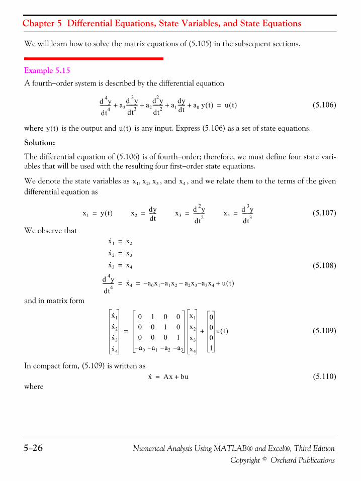
Chapter 5 Differential Equations, State Variables, and State Equations
5−26 Numerical Analysis Using MATLAB® and Excel®, Third EditionCopyright © Orchard Publications
We will learn how to solve the matrix equations of (5.105) in the subsequent sections.
Example 5.15 A fourth−order system is described by the differential equation
(5.106)
where is the output and is any input. Express (5.106) as a set of state equations.
Solution:
The differential equation of (5.106) is of fourth−order; therefore, we must define four state vari-ables that will be used with the resulting four first−order state equations.
We denote the state variables as , and , and we relate them to the terms of the givendifferential equation as
(5.107)
We observe that
(5.108)
and in matrix form
(5.109)
In compact form, (5.109) is written as(5.110)
where
d 4ydt4--------- a3
d 3ydt3--------- a2
d2ydt2-------- a1
dydt------ a0 y t( )+ + + + u t( )=
y t( ) u t( )
x1 x2 x3, , x4
x1 y t( )= x2dydt------= x3
d 2ydt2---------= x4
d 3ydt3---------=
x· 1 x2=
x· 2 x3=
x· 3 x4=
d 4ydt4--------- x· 4 a0x1– a1x2 a2x3–– a3x4– u t( )+= =
x· 1
x· 2
x· 3
x· 4
0 1 0 00 0 1 00 0 0 1a0– a1– a2– a3–
x1
x2
x3
x4
0001
u t( )+=
x· Ax bu+=
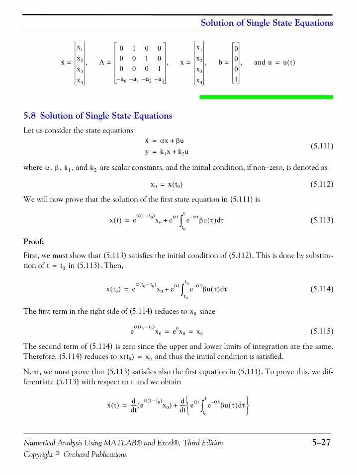
Numerical Analysis Using MATLAB® and Excel®, Third Edition 5−27Copyright © Orchard Publications
Solution of Single State Equations
5.8 Solution of Single State EquationsLet us consider the state equations
(5.111)
where , , , and are scalar constants, and the initial condition, if non−zero, is denoted as
(5.112)
We will now prove that the solution of the first state equation in (5.111) is
(5.113)
Proof:
First, we must show that (5.113) satisfies the initial condition of (5.112). This is done by substitu-tion of in (5.113). Then,
(5.114)
The first term in the right side of (5.114) reduces to since
(5.115)
The second term of (5.114) is zero since the upper and lower limits of integration are the same.Therefore, (5.114) reduces to and thus the initial condition is satisfied.
Next, we must prove that (5.113) satisfies also the first equation in (5.111). To prove this, we dif-ferentiate (5.113) with respect to and we obtain
x·
x· 1
x· 2
x· 3
x· 4
= A
0 1 0 00 0 1 00 0 0 1a0– a1– a2– a3–
= x
x1
x2
x3
x4
= b
0001
and u,=, , , u t( )=
x· αx βu+=
y k1x k2u+=
α β k1 k2
x0 x t0( )=
x t( ) eα t t0–( )
x0 eα t e ατ– βu τ( ) τdt0
t
∫+=
t t0=
x t0( ) eα t0 t0–( )
x0 eα t e α– τβu τ( ) τdt0
t0
∫+=
x0
eα t0 t0–( )
x0 e0x0 x0= =
x t0( ) x0=
t
x· t( ) ddt----- e
α t t0–( )x0( ) d
dt----- eαt e ατ– βu τ( ) τd
t0
t
∫⎩ ⎭⎨ ⎬⎧ ⎫
+=
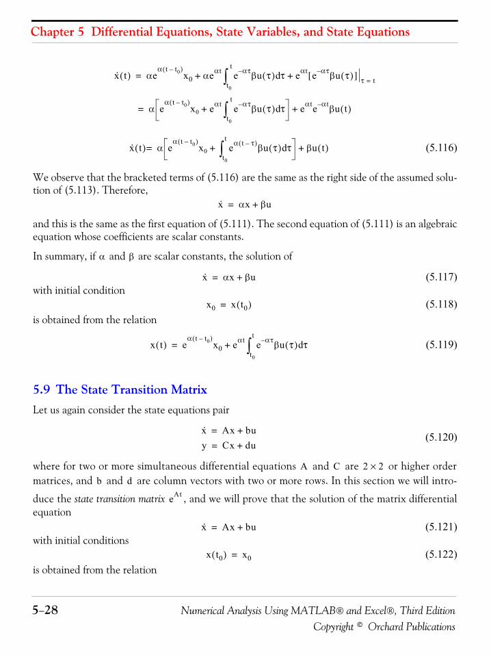
Chapter 5 Differential Equations, State Variables, and State Equations
5−28 Numerical Analysis Using MATLAB® and Excel®, Third EditionCopyright © Orchard Publications
(5.116)
We observe that the bracketed terms of (5.116) are the same as the right side of the assumed solu-tion of (5.113). Therefore,
and this is the same as the first equation of (5.111). The second equation of (5.111) is an algebraicequation whose coefficients are scalar constants.
In summary, if and are scalar constants, the solution of
(5.117)with initial condition
(5.118)is obtained from the relation
(5.119)
5.9 The State Transition Matrix Let us again consider the state equations pair
(5.120)
where for two or more simultaneous differential equations and are or higher ordermatrices, and and are column vectors with two or more rows. In this section we will intro-
duce the state transition matrix , and we will prove that the solution of the matrix differentialequation
(5.121)with initial conditions
(5.122)is obtained from the relation
x· t( ) αeα t t0–( )
x0 αeαt e ατ– βu τ( ) τ eαt e ατ– βu τ( )[ ] τ t=+d
t0
t
∫+=
α eα t t0–( )
x0 eαt e ατ– βu τ( ) τdt0
t
∫+ eα te α t– βu t( )+=
x· t( ) α eα t t0–( )
x0 eα t τ–( )βu τ( ) τdt0
t
∫+ βu t( )+=
x· αx βu+=
α β
x· αx βu+=
x0 x t0( )=
x t( ) eα t t0–( )
x0 eαt e α– τβu τ( ) τdt0
t
∫+=
x· Ax bu+=
y Cx du+=
A C 2 2×b d
eAt
x· Ax bu+=
x t0( ) x0=
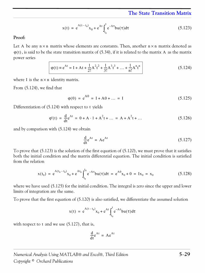
Numerical Analysis Using MATLAB® and Excel®, Third Edition 5−29Copyright © Orchard Publications
The State Transition Matrix
(5.123)
Proof:
Let be any matrix whose elements are constants. Then, another matrix denoted as, is said to be the state transition matrix of (5.34), if it is related to the matrix as the matrix
power series
(5.124)
where is the identity matrix.
From (5.124), we find that
(5.125)
Differentiation of (5.124) with respect to yields
(5.126)
and by comparison with (5.124) we obtain
(5.127)
To prove that (5.123) is the solution of the first equation of (5.120), we must prove that it satisfiesboth the initial condition and the matrix differential equation. The initial condition is satisfiedfrom the relation
(5.128)
where we have used (5.125) for the initial condition. The integral is zero since the upper and lowerlimits of integration are the same.
To prove that the first equation of (5.120) is also satisfied, we differentiate the assumed solution
with respect to and we use (5.127), that is,
x t( ) eA t t0–( )
x0 eAt e A– τbu τ( ) τdt0
t
∫+=
A n n× n n×ϕ t( ) A
ϕ t( ) eAt I At 12!-----A2t2 1
3!-----A3t3 … 1
n!-----Antn+ + + + +=≡
I n n×
ϕ 0( ) eA0 I A0 …+ + I= = =
t
ϕ' t( ) ddt-----eAt 0 A 1 A2t …+ +⋅+ A A2t …+ += = =
ddt-----eAt AeAt=
x t0( ) eA t0 t0–( )
x0 eAt0 e A– τbu τ( ) τd
t0
t0
∫+ eA0x0 0+ Ix0 x0= = = =
x t( ) eA t t0–( )
x0 eAt e A– τbu τ( ) τdt0
t
∫+=
t
ddt-----eAt AeAt=
Chapter 5 Differential Equations, State Variables, and State Equations
5−30 Numerical Analysis Using MATLAB® and Excel®, Third EditionCopyright © Orchard Publications
Then,
or
(5.129)
We recognize the bracketed terms in (5.129) as , and the last term as . Thus, the expres-sion (5.129) reduces to
In summary, if is an matrix whose elements are constants, , and is a column vec-tor with n elements, the solution of
(5.130)with initial condition
(5.131)is
(5.132)
Therefore, the solution of second or higher order systems using the state variable method, entails
the computation of the state transition matrix , and integration of (5.132).
5.10 Computation of the State Transition Matrix
Let be an matrix, and be the identity matrix. By definition, the eigenvalues , of are the roots of the nth order polynomial
(5.133)
We recall that expansion of a determinant produces a polynomial. The roots of the polynomial of(5.133) can be real (unequal or equal), or complex numbers.
Evaluation of the state transition matrix is based on the Cayley−Hamilton theorem. This theo-rem states that a matrix can be expressed as an degree polynomial in terms of the matrix
as
(5.134)
x· t( ) AeA t t0–( )
x0 AeAt e A– τbu τ( ) τdt0
t
∫ eAte A– tbu t( )+ +=
x· t( ) A eA t t0–( )
x0 eAt e A– τbu τ( ) τdt0
t
∫+ eAte A– tbu t( )+=
x t( ) bu t( )
x· t( ) Ax bu+=
A n n× n 2≥ b
x· t( ) Ax bu+=
x0 x t0( )=
x t( ) eA t t0–( )
x0 eAt e A– τbu τ( ) τdt0
t
∫+=
eAt
eAt
A n n× I n n× λi
i 1 2 … n, , ,= A
det A λI–[ ] 0=
eAt
n 1–( )thA
eAt a0I a1A a2A2 … an 1– An 1–+ + + +=
Numerical Analysis Using MATLAB® and Excel®, Third Edition 5−31Copyright © Orchard Publications
Computation of the State Transition Matrix
where the coefficients are functions of the eigenvalues . We accept (5.134) without provingit. The proof can be found in Linear Algebra and Matrix Theory textbooks.
Since the coefficients are functions of the eigenvalues , we must consider the following cases:
Case I: Distinct Eigenvalues (Real or Complex)
If , that is, if all eigenvalues of a given matrix are distinct, thecoefficients are found from the simultaneous solution of the following system of equa-tions:
(5.135)
Example 5.16
Compute the state transition matrix given that
Solution:
We must first find the eigenvalues of the given matrix . These are found from the expansionof
For this example,
or
Therefore,(5.136)
Next, we must find the coefficients of (5.134). Since is a matrix, we only need to con-sider the first two terms of that relation, that is,
ai λ
ai λ
λ1 λ2 λ3 … λn≠ ≠ ≠ ≠ A
ai
a0 a1λ1 a2λ12 … an 1– λ1
n 1–+ + + + eλ1t
=
a0 a1λ2 a2λ22 … an 1– λ2
n 1–+ + + + eλ2t
=
…
a0 a1λn a2λn2 … an 1– λn
n 1–+ + + + eλnt
=
eAt A 2– 10 1–
=
λ A
det A λI–[ ] 0=
det A λI–[ ] det 2– 10 1–
λ 1 00 1
–⎩ ⎭⎨ ⎬⎧ ⎫
det 2– λ– 10 1– λ–
0= = =
2– λ–( ) 1– λ–( ) 0==
λ 1+( ) λ 2+( ) 0=
λ1 1 and λ2 2–=–=
ai A 2 2×
Chapter 5 Differential Equations, State Variables, and State Equations
5−32 Numerical Analysis Using MATLAB® and Excel®, Third EditionCopyright © Orchard Publications
(5.137)
The coefficients and are found from (5.135). For this example,
or
(5.138)
Simultaneous solution of (5.138) yields
(5.139)
and by substitution into (5.137),
or
(5.140)
In summary, we compute the state transition matrix for a given matrix using the followingprocedure:1. We find the eigenvalues from . We can write at once by subtract-
ing from each of the main diagonal elements of . If the dimension of is a matrix,it will yield two eigenvalues; if it is a matrix, it will yield three eigenvalues, and so on. Ifthe eigenvalues are distinct, we perform steps 2 through 4 below; otherwise we refer to CaseII.
2. If the dimension of is a matrix, we use only the first 2 terms of the right side of thestate transition matrix
(5.141)
If matrix is a matrix, we use the first 3 terms, and so on.
eAt a0I a1A+=
a0 a1
a0 a1λ1+ eλ1t
=
a0 a1λ2+ eλ2t
=
a0 a1 1–( )+ e t–=
a0 a1 2–( )+ e 2t–=
a0 2e t– e 2t––=
a1 e t– e 2t––=
eAt 2e t– e 2t––( ) 1 00 1
e t– e 2t––( ) 2– 10 1–
+=
eAt e 2t– e t– e 2t––
0 e t–=
eAt A
λ det A λI–[ ] 0= A λI–[ ]λ A A 2 2×
3 3×
A 2 2×
eAt a0I a1A a2A2 … an 1– An 1–+ + + +=
A 3 3×
Numerical Analysis Using MATLAB® and Excel®, Third Edition 5−33Copyright © Orchard Publications
Computation of the State Transition Matrix
3. We obtain the coefficients from
We use as many equations as the number of the eigenvalues, and we solve for the coefficients.
4. We substitute the coefficients into the state transition matrix of (5.141), and we simplify.
Example 5.17
Compute the state transition matrix given that
(5.142)
Solution:
1. We first compute the eigenvalues from . We obtain at once, by sub-tracting from each of the main diagonal elements of . Then,
(5.143)
and expansion of this determinant yields the polynomial
(5.144)
We will use MATLAB roots(p) function to obtain the roots of (5.144).
p=[1 −6 11 −6]; r=roots(p); fprintf(' \n'); fprintf('lambda1 = %5.2f \t', r(1));...fprintf('lambda2 = %5.2f \t', r(2)); fprintf('lambda3 = %5.2f', r(3))
lambda1 = 3.00 lambda2 = 2.00 lambda3 = 1.00
and thus the eigenvalues are
ai
a0 a1λ1 a2λ12 … an 1– λ1
n 1–+ + + + eλ1t
=
a0 a1λ2 a2λ22 … an 1– λ2
n 1–+ + + + eλ2t
=
…
a0 a1λn a2λn2 … an 1– λn
n 1–+ + + + eλnt
=
ai
ai
eAt
A5 7 5–0 4 1–2 8 3–
=
det A λI–[ ] 0= A λI–[ ]λ A
det A λI–[ ] det5 λ– 7 5–
0 4 λ– 1–2 8 3– λ–
0= =
λ3 6λ2 11λ 6–+– 0=
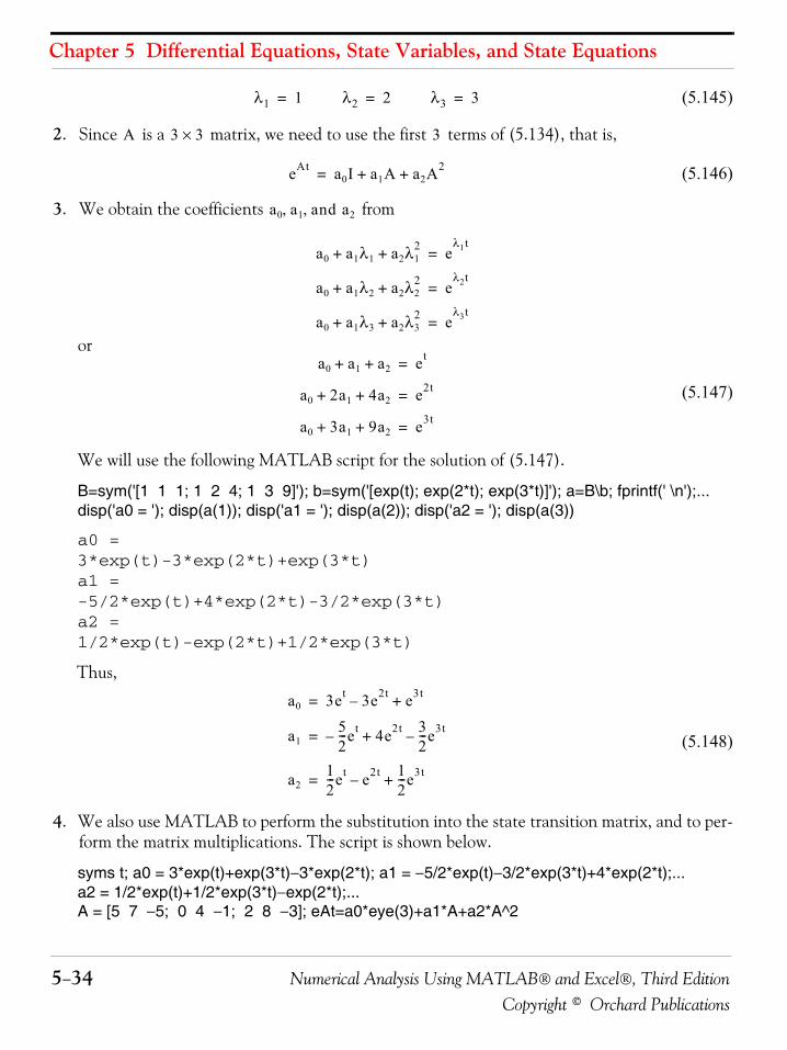
Chapter 5 Differential Equations, State Variables, and State Equations
5−34 Numerical Analysis Using MATLAB® and Excel®, Third EditionCopyright © Orchard Publications
(5.145)
2. Since is a matrix, we need to use the first terms of (5.134), that is,
(5.146)
3. We obtain the coefficients from
or
(5.147)
We will use the following MATLAB script for the solution of (5.147).
B=sym('[1 1 1; 1 2 4; 1 3 9]'); b=sym('[exp(t); exp(2*t); exp(3*t)]'); a=B\b; fprintf(' \n');...disp('a0 = '); disp(a(1)); disp('a1 = '); disp(a(2)); disp('a2 = '); disp(a(3))
a0 = 3*exp(t)-3*exp(2*t)+exp(3*t)a1 = -5/2*exp(t)+4*exp(2*t)-3/2*exp(3*t)a2 = 1/2*exp(t)-exp(2*t)+1/2*exp(3*t)
Thus,
(5.148)
4. We also use MATLAB to perform the substitution into the state transition matrix, and to per-form the matrix multiplications. The script is shown below.
syms t; a0 = 3*exp(t)+exp(3*t)−3*exp(2*t); a1 = −5/2*exp(t)−3/2*exp(3*t)+4*exp(2*t);...a2 = 1/2*exp(t)+1/2*exp(3*t)−exp(2*t);...A = [5 7 −5; 0 4 −1; 2 8 −3]; eAt=a0*eye(3)+a1*A+a2*A^2
λ1 1= λ2 2= λ3 3=
A 3 3× 3
eAt a0I a1A a2A2+ +=
a0 a1 and a2, ,
a0 a1λ1 a2λ12+ + e
λ1t=
a0 a1λ2 a2λ22+ + e
λ2t=
a0 a1λ3 a2λ32+ + e
λ3t=
a0 a1 a2+ + et=
a0 2a1 4a2+ + e2t=
a0 3a1 9a2+ + e3t=
a0 3et 3e2t– e3t+=
a152---et– 4e2t 3
2---e3t–+=
a212---et e2t–
12---e3t+=
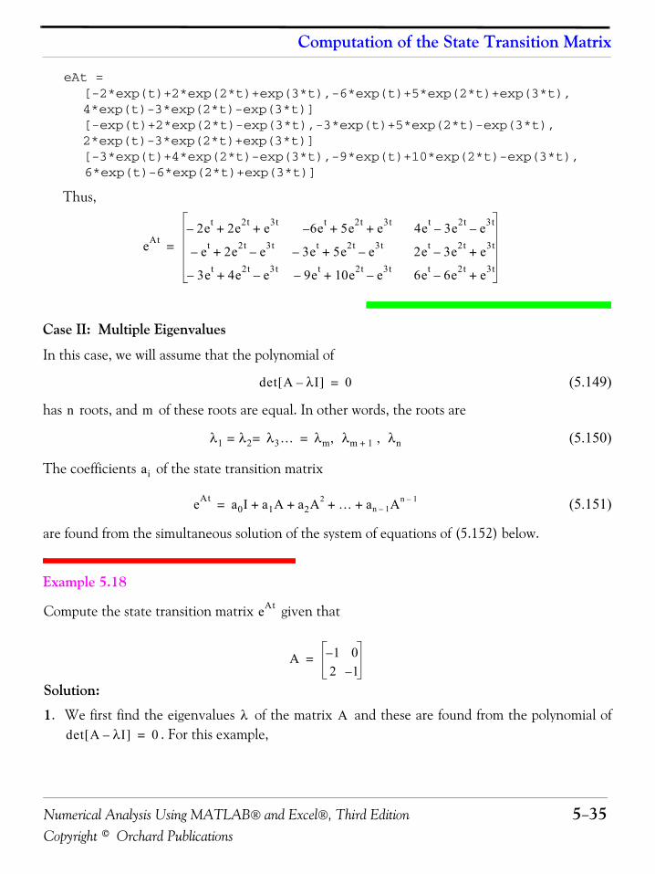
Numerical Analysis Using MATLAB® and Excel®, Third Edition 5−35Copyright © Orchard Publications
Computation of the State Transition Matrix
eAt =[-2*exp(t)+2*exp(2*t)+exp(3*t),-6*exp(t)+5*exp(2*t)+exp(3*t),4*exp(t)-3*exp(2*t)-exp(3*t)][-exp(t)+2*exp(2*t)-exp(3*t),-3*exp(t)+5*exp(2*t)-exp(3*t),2*exp(t)-3*exp(2*t)+exp(3*t)][-3*exp(t)+4*exp(2*t)-exp(3*t),-9*exp(t)+10*exp(2*t)-exp(3*t),6*exp(t)-6*exp(2*t)+exp(3*t)]
Thus,
Case II: Multiple Eigenvalues
In this case, we will assume that the polynomial of
(5.149)
has roots, and of these roots are equal. In other words, the roots are
(5.150)
The coefficients of the state transition matrix
(5.151)
are found from the simultaneous solution of the system of equations of (5.152) below.
Example 5.18
Compute the state transition matrix given that
Solution:
1. We first find the eigenvalues of the matrix and these are found from the polynomial of. For this example,
eAt2et– 2e2t e3t+ + 6– et 5e2t e3t+ + 4et 3e2t– e3t–
et– 2e2t e3t–+ 3et– 5e2t e3t–+ 2et 3e2t– e3t+
3et– 4e2t e3t–+ 9et– 10e2t e3t–+ 6et 6e2t– e3t+
=
det A λI–[ ] 0=
n m
λ1 λ2= λ3= … λm, λm 1+ , λn=
ai
eAt a0I a1A a2A2 … an 1– An 1–+ + + +=
eAt
A 1– 02 1–
=
λ Adet A λI–[ ] 0=
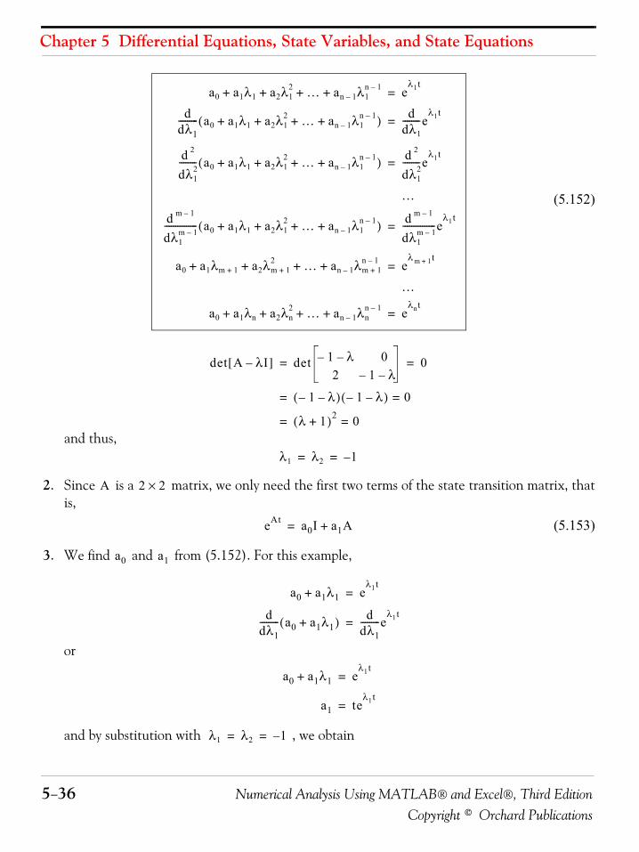
Chapter 5 Differential Equations, State Variables, and State Equations
5−36 Numerical Analysis Using MATLAB® and Excel®, Third EditionCopyright © Orchard Publications
(5.152)
and thus,
2. Since is a matrix, we only need the first two terms of the state transition matrix, thatis,
(5.153)
3. We find and from (5.152). For this example,
or
and by substitution with , we obtain
a0 a1λ1 a2λ12 … an 1– λ1
n 1–+ + + + eλ1t
=
ddλ1--------- a0 a1λ1 a2λ1
2 … an 1– λ1n 1–+ + + +( ) d
dλ1--------e
λ1t=
d 2
dλ12
-------- a0 a1λ1 a2λ12 … an 1– λ1
n 1–+ + + +( ) d 2
dλ12
--------eλ1t
=
…
d m 1–
dλ1m 1–
--------------- a0 a1λ1 a2λ12 … an 1– λ1
n 1–+ + + +( ) d m 1–
dλ1m 1–
---------------eλ1t
=
a0 a1λm 1+ a2λm 1+2 … an 1– λm 1+
n 1–+ + + + eλ m 1+ t
=
…
a0 a1λn a2λn2 … an 1– λn
n 1–+ + + + eλnt
=
det A λI–[ ] det 1– λ– 02 1– λ–
0= =
1– λ–( ) 1– λ–( ) 0==
λ 1+( )2 0==
λ1 λ2 1–= =
A 2 2×
eAt a0I a1A+=
a0 a1
a0 a1λ1+ eλ1t
=
ddλ1--------- a0 a1λ1+( ) d
dλ1---------e
λ1t=
a0 a1λ1+ eλ1t
=
a1 teλ1t
=
λ1 λ2 1–= =
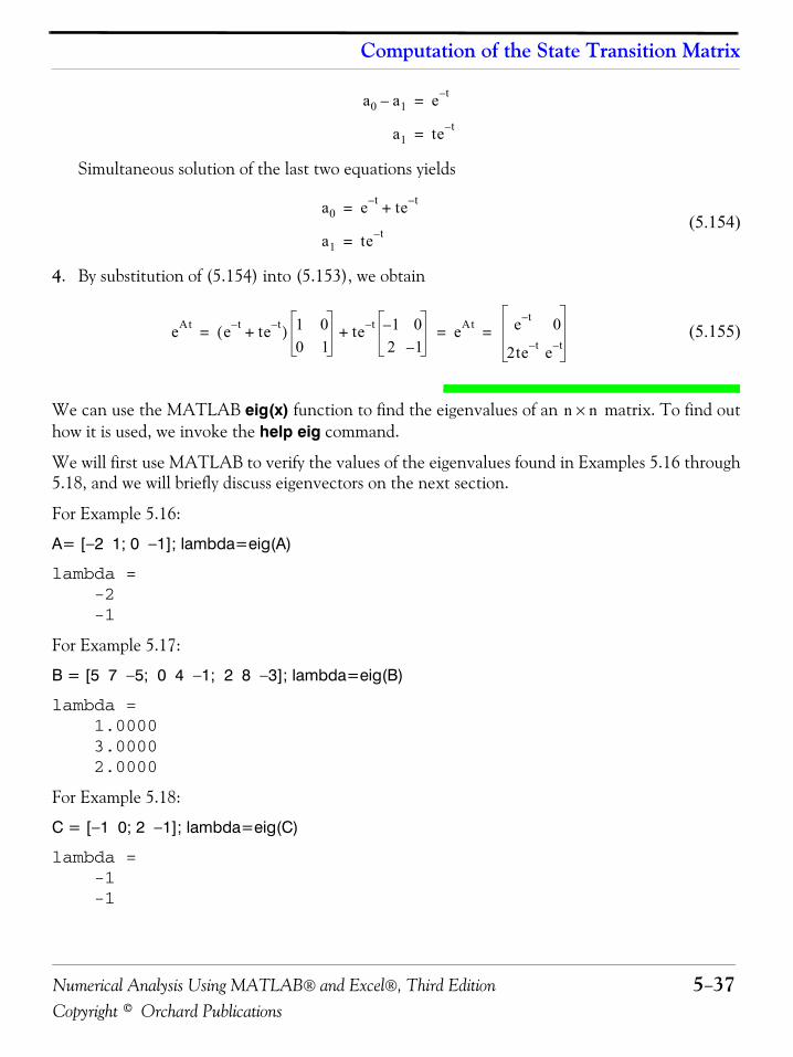
Numerical Analysis Using MATLAB® and Excel®, Third Edition 5−37Copyright © Orchard Publications
Computation of the State Transition Matrix
Simultaneous solution of the last two equations yields
(5.154)
4. By substitution of (5.154) into (5.153), we obtain
(5.155)
We can use the MATLAB eig(x) function to find the eigenvalues of an matrix. To find outhow it is used, we invoke the help eig command.
We will first use MATLAB to verify the values of the eigenvalues found in Examples 5.16 through5.18, and we will briefly discuss eigenvectors on the next section.
For Example 5.16:
A= [−2 1; 0 −1]; lambda=eig(A)
lambda = -2 -1
For Example 5.17:
B = [5 7 −5; 0 4 −1; 2 8 −3]; lambda=eig(B)
lambda = 1.0000 3.0000 2.0000
For Example 5.18:
C = [−1 0; 2 −1]; lambda=eig(C)
lambda = -1 -1
a0 a1– e t–=
a1 te t–=
a0 e t– te t–+=
a1 te t–=
eAt e t– te t–+( ) 1 00 1
te t– 1– 02 1–
+ eAt e t– 0
2te t– e t–= = =
n n×
Chapter 5 Differential Equations, State Variables, and State Equations
5−38 Numerical Analysis Using MATLAB® and Excel®, Third EditionCopyright © Orchard Publications
5.11 EigenvectorsConsider the relation
(5.156)
where is an matrix, is a column vector, and is a scalar number. We can express thisrelation in matrix form as
(5.157)
We write (5.157) as(5.158)
or
(5.159)
The equations of (5.159) will have non−trivial solutions if and only if its determinant is zero*, thatis, if
(5.160)
Expansion of the determinant of (5.160) results in a polynomial equation of degree in , and itis called the characteristic equation.
We can express (5.160) in a compact form as
(5.161)
As we know, the roots of the characteristic equation are the eigenvalues of the matrix , andcorresponding to each eigenvalue , there is a non−trivial solution of the column vector , i.e.,
*. This is because we want the vector X in (5.158) to be a non−zero vector and the product to be zero.
AX λX=
A n n× X λ
a11 a12 … a1n
a21 a22 … a2n
… … … …an1 an2 … ann
x1
x2
…xn
λ
x1
x2
…xn
=
A λI–( )X 0=
a11 λ–( )x1 a12x2 … a1nxn
a21x1 a22 λ–( )x2 … a2nxn
… … … …an1x1 an2x2 … ann λ–( )xn
0=
A λI–( )X
det
a11 λ–( ) a12 … a1n
a21 a22 λ–( ) … a2n
… … … …an1 an2 … ann λ–( )
0=
n λ
det A λI–( ) 0=
λ Aλ X
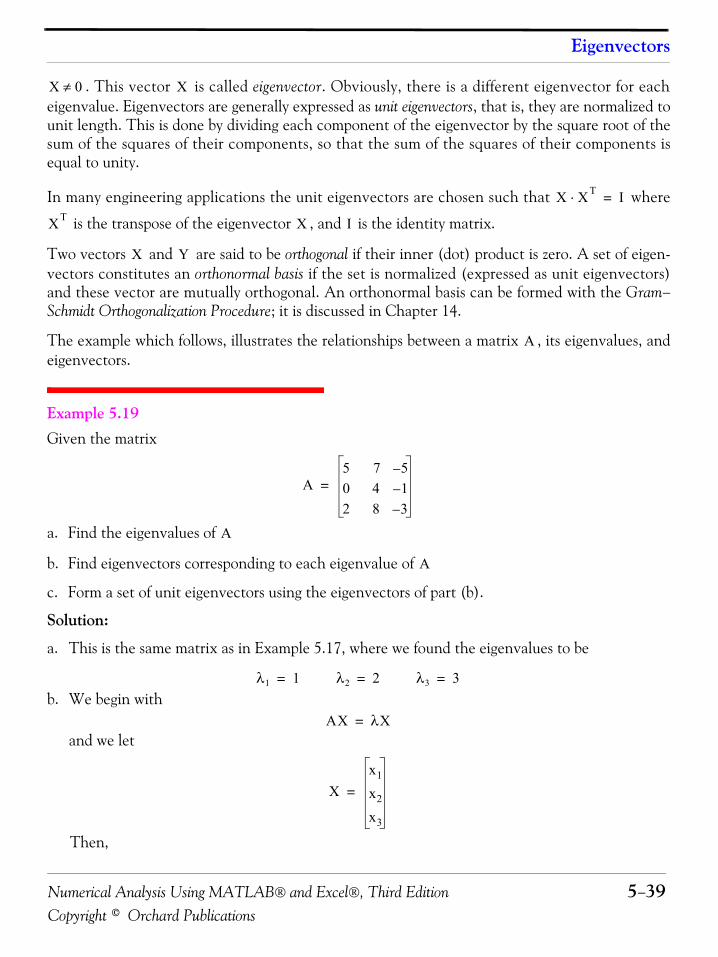
Numerical Analysis Using MATLAB® and Excel®, Third Edition 5−39Copyright © Orchard Publications
Eigenvectors
. This vector is called eigenvector. Obviously, there is a different eigenvector for eacheigenvalue. Eigenvectors are generally expressed as unit eigenvectors, that is, they are normalized tounit length. This is done by dividing each component of the eigenvector by the square root of thesum of the squares of their components, so that the sum of the squares of their components isequal to unity.
In many engineering applications the unit eigenvectors are chosen such that where
is the transpose of the eigenvector , and is the identity matrix.
Two vectors and are said to be orthogonal if their inner (dot) product is zero. A set of eigen-vectors constitutes an orthonormal basis if the set is normalized (expressed as unit eigenvectors)and these vector are mutually orthogonal. An orthonormal basis can be formed with the Gram−Schmidt Orthogonalization Procedure; it is discussed in Chapter 14.
The example which follows, illustrates the relationships between a matrix , its eigenvalues, andeigenvectors.
Example 5.19 Given the matrix
a. Find the eigenvalues of
b. Find eigenvectors corresponding to each eigenvalue of
c. Form a set of unit eigenvectors using the eigenvectors of part (b).
Solution:
a. This is the same matrix as in Example 5.17, where we found the eigenvalues to be
b. We begin with
and we let
Then,
X 0≠ X
X XT⋅ I=
XT X I
X Y
A
A5 7 5–0 4 1–2 8 3–
=
A
A
λ1 1= λ2 2= λ3 3=
AX λX=
Xx1
x2
x3
=
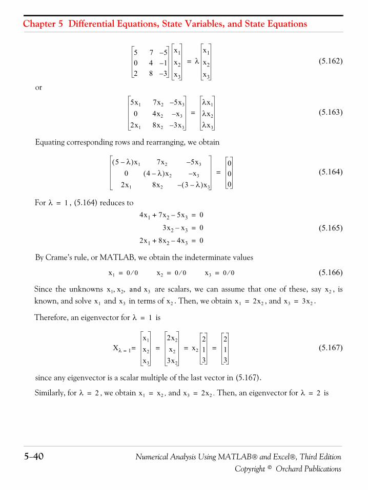
Chapter 5 Differential Equations, State Variables, and State Equations
5−40 Numerical Analysis Using MATLAB® and Excel®, Third EditionCopyright © Orchard Publications
(5.162)
or
(5.163)
Equating corresponding rows and rearranging, we obtain
(5.164)
For , (5.164) reduces to
(5.165)
By Crame’s rule, or MATLAB, we obtain the indeterminate values
(5.166)
Since the unknowns are scalars, we can assume that one of these, say , isknown, and solve and in terms of . Then, we obtain , and .
Therefore, an eigenvector for is
(5.167)
since any eigenvector is a scalar multiple of the last vector in (5.167).
Similarly, for , we obtain , and . Then, an eigenvector for is
5 7 5–0 4 1–2 8 3–
x1
x2
x3
λx1
x2
x3
=
5x1 7x2 5x3–
0 4x2 x3–
2x1 8x2 3x3–
λx1
λx2
λx3
=
5 λ–( )x1 7x2 5x3–
0 4 λ–( )x2 x3–
2x1 8x2 3 λ–( )x3–
000
=
λ 1=
4x1 7x2 5x3–+ 0=
3x2 x3– 0=
2x1 8x2 4x3–+ 0=
x1 0 0⁄= x2 0 0⁄= x3 0 0⁄=
x1 x2 and x3, , x2
x1 x3 x2 x1 2x2= x3 3x2=
λ 1=
Xλ 1=
x1
x2
x3
=2x2
x2
3x2
x2
213
213
= = =
λ 2= x1 x2= x3 2x2= λ 2=
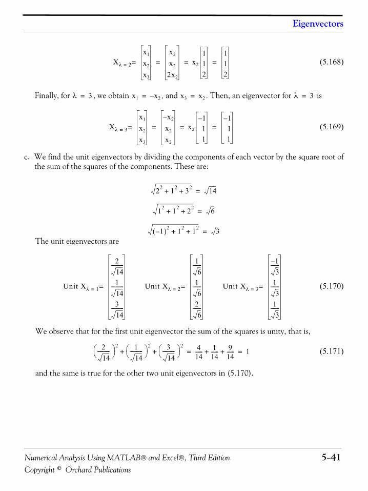
Numerical Analysis Using MATLAB® and Excel®, Third Edition 5−41Copyright © Orchard Publications
Eigenvectors
(5.168)
Finally, for , we obtain , and . Then, an eigenvector for is
(5.169)
c. We find the unit eigenvectors by dividing the components of each vector by the square root ofthe sum of the squares of the components. These are:
The unit eigenvectors are
(5.170)
We observe that for the first unit eigenvector the sum of the squares is unity, that is,
(5.171)
and the same is true for the other two unit eigenvectors in (5.170).
Xλ 2=
x1
x2
x3
=x2
x2
2x2
x2
112
112
= = =
λ 3= x1 x– 2= x3 x2= λ 3=
Xλ 3=
x1
x2
x3
=x– 2
x2
x2
x2
1–11
1–11
= = =
22 12 32+ + 14=
12 12 22+ + 6=
1–( )2 12 12+ + 3=
Unit Xλ 1=
214
----------
114
----------
314
----------
= Unit Xλ 2=
16
-------
16
-------
26
-------
= Unit Xλ 3=
1–
3-------
13
-------
13
-------
=
214
----------⎝ ⎠⎛ ⎞ 2 1
14----------⎝ ⎠⎛ ⎞ 2 3
14----------⎝ ⎠⎛ ⎞ 2
+ + 414------ 1
14------ 9
14------+ + 1= =
Chapter 5 Differential Equations, State Variables, and State Equations
5−42 Numerical Analysis Using MATLAB® and Excel®, Third EditionCopyright © Orchard Publications
5.12 Summary• Differential equations are classified by:
Type − Ordinary or Partial
Order − The highest order derivative which is included in the differential equation
Degree − The exponent of the highest power of the highest order derivative after the differen-tial equation has been cleared of any fractions or radicals in the dependent variable and itsderivatives
• If the dependent variable is a function of only a single variable , that is, if , thedifferential equation which relates and is said to be an ordinary differential equation andit is abbreviated as ODE.
• If the dependent variable is a function of two or more variables such as , where and are independent variables, the differential equation that relates , , and is said to bea partial differential equation and it is abbreviated as PDE.
• A function is a solution of a differential equation if the latter is satisfied when andits derivatives are replaced throughout by and its corresponding derivatives. Also, theinitial conditions must be satisfied.
• The ODE
is a non−homogeneous differential equation if the right side, known as forcing function, is notzero. If the forcing function is zero, the differential equation is referred to as homogeneous dif-ferential equation.
• The most general solution of an homogeneous ODE is the linear combination
where the subscript is used to denote homogeneous and are arbitrary con-stants.
• Generally, in engineering the solution of the homogeneous ODE, also known as the comple-mentary solution, is referred to as the natural response, and is denoted as or simply .The particular solution of a non−homogeneous ODE is be referred to as the forced response,and is denoted as or simply . The total solution of the non−homogeneous ODE is thesummation of the natural and forces responses, that is,
y x y f x( )=
y x
y y f x t,( )= xt y x t
y f x( )= yf x( )
and nydtn--------- an 1–
d n 1– ydt n 1–---------------- … a1
dydt------ a0 y+ + + + bm
d mxdt m---------- bm 1–
d m 1– xdt n 1–----------------- … b1
dxdt------ b0x+ + + +=
yH t( ) k1 y1 t( ) k2 y2 t( ) k3 y3 t( ) … kn yn t( )+ + + +=
H k1 k2 k3 … kn, , , ,
yN t( ) yN
yF t( ) yF
Numerical Analysis Using MATLAB® and Excel®, Third Edition 5−43Copyright © Orchard Publications
Summary
The natural response contains arbitrary constants and these can be evaluated from thegiven initial conditions. The forced response , however, contains no arbitrary constants. It isimperative to remember that the arbitrary constants of the natural response must be evaluatedfrom the total response.
• For an order homogeneous differential equation the solutions are
where are the solutions of the characteristic equation
and are the constant coefficients of the ODE
• If the roots of the characteristic equation are distinct, the solutions of the natural responseare independent and the most general solution is:
• If the solution of the characteristic equation contains equal roots, the most general solutionhas the form:
• If the characteristic equation contains complex roots, these occur as complex conjugate pairs.Thus, if one root is where and are real numbers, then another root is
. Then, for two complex conjugate roots we evaluate the constants from theexpressions
• The forced response of a non−homogeneous ODE can be found by the method of undeter-mined coefficients or the method of variation of parameters.
• With the method of undetermined coefficients, the forced response is a function similar to theright side of the non−homogeneous ODE. The form of the forced response for second ordernon−homogeneous ODEs is given in Table 5.1.
• In certain non−homogeneous ODEs, the right side cannot be determined by the methodof undetermined coefficients. For these ODEs we must use the method of variation of parame-
y t( ) y NaturalResponse
y ForcedResponse
+ yN yF+= =
yN
yF
nth
y1 k1es1t
= y2 k2es2t
= y3 k3es3t
= … yn knesnt
=, , , ,
s1 s2 … sn, , ,
an sn an 1– sn 1– … a1 s a0+ + + + 0=
an an 1– … a1 a0, , , ,
n
yN k1es1t
= k2es2t
… knesnt
+ + +
m
yN k1 k2t … kmtm 1–+ + +( ) es1t
= kn i– es2t
… knesnt
+ + +
s1 α– jβ+= α β
s2 α– j– β=
k1es1t
k2es2t
+ e α t– k3 βtcos k4 βsin t+( ) e α t– k5 βt ϕ+( )cos==
f t( )
Chapter 5 Differential Equations, State Variables, and State Equations
5−44 Numerical Analysis Using MATLAB® and Excel®, Third EditionCopyright © Orchard Publications
ters. This method will work with all linear equations including those with variable coefficientsprovided that the general form of the natural response is known.
• For second order ODEs with constant coefficients, the method of variation of parametersreplaces the constants and by two variables and that satisfy the following threerelations:
Simultaneous solution of last two expressions above will yield the values of and; then, integration of these will produce and , which when substituted into the
first will yield the total solution.
• An nth−order differential equation can be resolved to first−order simultaneous differentialequations with a set of auxiliary variables called state variables. The resulting first−order differ-ential equations are called state space equations, or simply state equations.
• The state representation of a system can be described by the pair of the of the state spaceequations
• In a system of state equations of the form
where , , , and are scalar constants, and the initial condition, if non−zero is denotedas , the solution of the first state equation above is
• In a system of state equations of the form
k1 k2 u1 u2
y u1 y1 u2 y2+=
du1dt------- y1
du2dt
-------- y2+ 0=
du1dt
--------dy1dt
--------⋅du2dt
--------dy2dt
--------⋅+ f t( )=
du1 dt⁄
du2 dt⁄ u1 u2
n
x· Ax bu+=
y Cx du+=
x· αx βu+=
y k1x k2u+=
α β k1 k2
x0 x t0( )=
x t( ) eα t t0–( )
x0 eαt e ατ– βu τ( ) τdt0
t
∫+=
x· Ax bu+=
y Cx du+=
Numerical Analysis Using MATLAB® and Excel®, Third Edition 5−45Copyright © Orchard Publications
Summary
where for two or more simultaneous differential equations and are or higher ordermatrices, and and are column vectors with two or more rows, the solution of the matrixdifferential equation with initial conditions is obtained from therelation
where the state transition matrix is defined as the matrix power series
and is the identity matrix.
• If is an matrix, and be the identity matrix, the eigenvalues , of are the roots of the nth order polynomial
• Evaluation of the state transition matrix is based on the Cayley−Hamilton theorem. Thistheorem states that a matrix can be expressed as an degree polynomial in terms of thematrix as
where the coefficients are functions of the eigenvalues .
• If , that is, if all eigenvalues of a given matrix are distinct, the coeffi-cients are found from the simultaneous solution of the following system of equations:
• If the polynomial of has roots, and of these roots are equal, that is, if, the coefficients of the state transition matrix
A C 2 2×b d
x· Ax bu+= x t0( ) x0=
x t( ) eA t t0–( )
x0 eAt e A– τbu τ( ) τdt0
t
∫+=
eAt
ϕ t( ) eAt I At 12!-----A2t2 1
3!-----A3t3 … 1
n!-----Antn+ + + + +=≡
I n n×
A n n× I n n× λi i 1 2 … n, , ,=
A
det A λI–[ ] 0=
eAt
n 1–( )thA
eAt a0I a1A a2A2 … an 1– An 1–+ + + +=
ai λ
λ1 λ2 λ3 … λn≠ ≠ ≠ ≠ A
ai
a0 a1λ1 a2λ12 … an 1– λ1
n 1–+ + + + eλ1t
=
a0 a1λ2 a2λ22 … an 1– λ2
n 1–+ + + + eλ2t
=
…
a0 a1λn a2λn2 … an 1– λn
n 1–+ + + + eλnt
=
det A λI–[ ] 0= n mλ1 λ2= λ3= … λm, λm 1+ , λn= ai
eAt a0I a1A a2A2 … an 1– An 1–+ + + +=
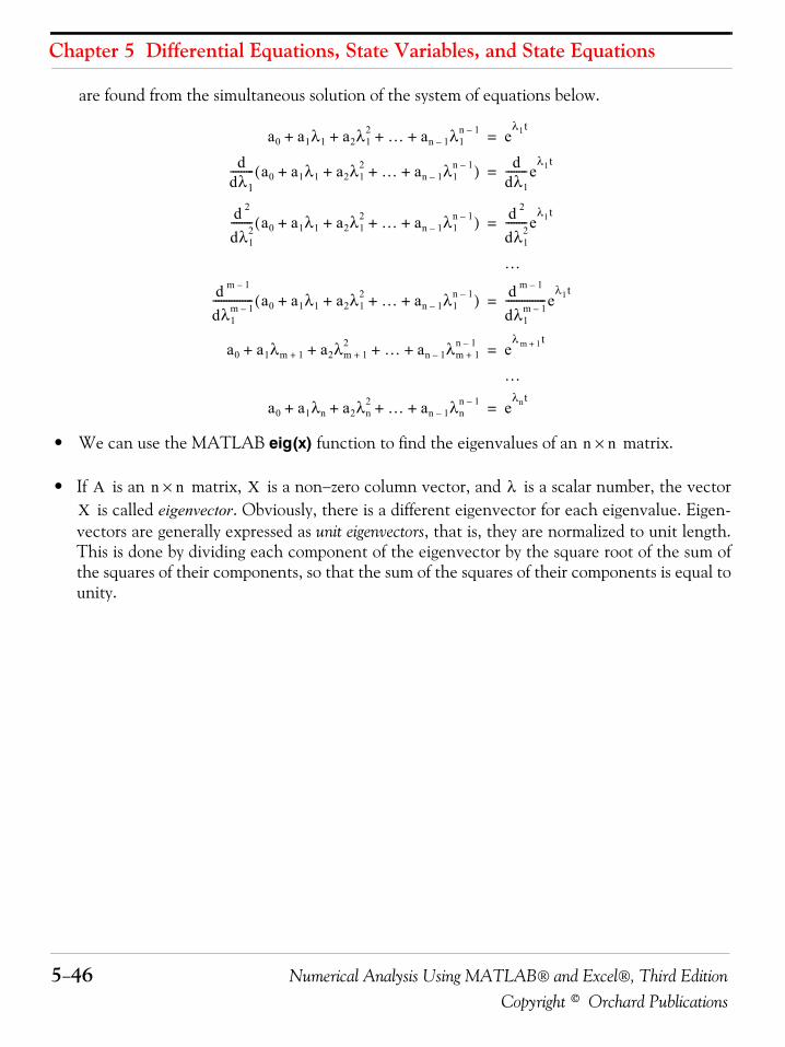
Chapter 5 Differential Equations, State Variables, and State Equations
5−46 Numerical Analysis Using MATLAB® and Excel®, Third EditionCopyright © Orchard Publications
are found from the simultaneous solution of the system of equations below.
• We can use the MATLAB eig(x) function to find the eigenvalues of an matrix.
• If is an matrix, is a non−zero column vector, and is a scalar number, the vector is called eigenvector. Obviously, there is a different eigenvector for each eigenvalue. Eigen-
vectors are generally expressed as unit eigenvectors, that is, they are normalized to unit length.This is done by dividing each component of the eigenvector by the square root of the sum ofthe squares of their components, so that the sum of the squares of their components is equal tounity.
a0 a1λ1 a2λ12 … an 1– λ1
n 1–+ + + + eλ1t
=
ddλ1--------- a0 a1λ1 a2λ1
2 … an 1– λ1n 1–+ + + +( ) d
dλ1--------e
λ1t=
d 2
dλ12
-------- a0 a1λ1 a2λ12 … an 1– λ1
n 1–+ + + +( ) d 2
dλ12
--------eλ1t
=
…
d m 1–
dλ1m 1–
--------------- a0 a1λ1 a2λ12 … an 1– λ1
n 1–+ + + +( ) d m 1–
dλ1m 1–
---------------eλ1t
=
a0 a1λm 1+ a2λm 1+2 … an 1– λm 1+
n 1–+ + + + eλ m 1+ t
=
…
a0 a1λn a2λn2 … an 1– λn
n 1–+ + + + eλnt
=
n n×
A n n× X λX
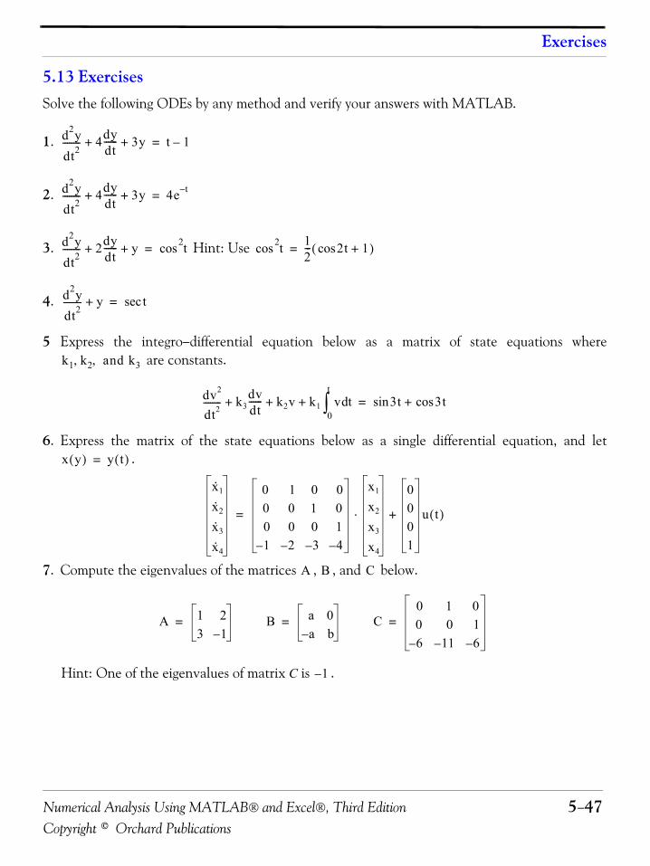
Numerical Analysis Using MATLAB® and Excel®, Third Edition 5−47Copyright © Orchard Publications
Exercises
5.13 ExercisesSolve the following ODEs by any method and verify your answers with MATLAB.
1.
2.
3. Hint: Use
4.
5 Express the integro−differential equation below as a matrix of state equations where are constants.
6. Express the matrix of the state equations below as a single differential equation, and let.
7. Compute the eigenvalues of the matrices , , and below.
Hint: One of the eigenvalues of matrix C is .
d2ydt2-------- 4dy
dt------ 3y+ + t 1–=
d2ydt2-------- 4dy
dt------ 3y+ + 4e t–=
d2ydt2-------- 2dy
dt------ y+ + t2cos= t2cos 1
2--- 2t 1+cos( )=
d2ydt2-------- y+ tsec=
k1 k2 and k3, ,
dv2
dt2-------- k3
dvdt------ k2v k1 v td
0
t
∫+ + + 3tsin 3tcos+=
x y( ) y t( )=
x· 1
x· 2
x· 3
x· 4
0 1 0 00 0 1 00 0 0 11– 2– 3– 4–
x1
x2
x3
x4
⋅
0001
u t( )+=
A B C
A 1 23 1–
= B a 0a– b
= C0 1 00 0 16– 11– 6–
=
1–
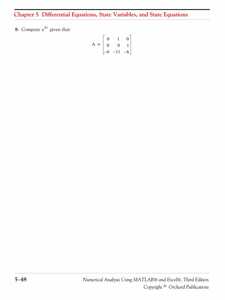
Chapter 5 Differential Equations, State Variables, and State Equations
5−48 Numerical Analysis Using MATLAB® and Excel®, Third EditionCopyright © Orchard Publications
8. Compute given thateAt
A0 1 00 0 16– 11– 6–
=
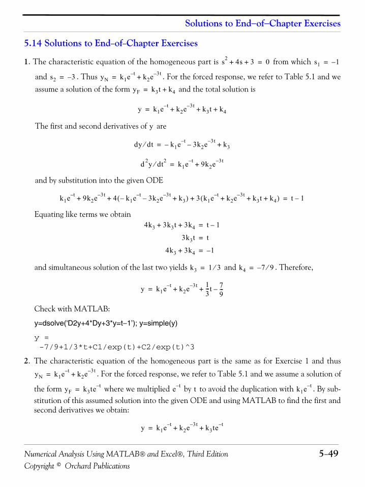
Numerical Analysis Using MATLAB® and Excel®, Third Edition 5−49Copyright © Orchard Publications
Solutions to End−of−Chapter Exercises
5.14 Solutions to End−of−Chapter Exercises
1. The characteristic equation of the homogeneous part is from which
and . Thus . For the forced response, we refer to Table 5.1 and weassume a solution of the form and the total solution is
The first and second derivatives of are
and by substitution into the given ODE
Equating like terms we obtain
and simultaneous solution of the last two yields and . Therefore,
Check with MATLAB:
y=dsolve('D2y+4*Dy+3*y=t−1’); y=simple(y)
y = -7/9+1/3*t+C1/exp(t)+C2/exp(t)^3
2. The characteristic equation of the homogeneous part is the same as for Exercise 1 and thus
. For the forced response, we refer to Table 5.1 and we assume a solution of
the form where we multiplied by to avoid the duplication with . By sub-stitution of this assumed solution into the given ODE and using MATLAB to find the first andsecond derivatives we obtain:
s2 4s 3+ + 0= s1 1–=
s2 3–= yN k1e t– k2e 3t–+=
yF k3t k4+=
y k1e t– k2e 3t– k3t k4+ + +=
y
dy dt⁄ k1e t–– 3k2e 3t–– k3+=
d 2y dt2⁄ k1e t– 9k2e 3t–+=
k1e t– 9k2e 3t– 4 k1e t–– 3k2e 3t–– k3+( ) 3 k1e t– k2e 3t– k3t k4+ + +( )+ + + t 1–=
4k3 3k3t 3k4+ + t 1–=
3k3t t=
4k3 3k4+ 1–=
k3 1 3⁄= k4 7 9⁄–=
y k1e t– k2e 3t– 13---t 7
9---–+ +=
yN k1e t– k2e 3t–+=
yF k3te t–= e t– t k1e t–
y k1e t– k2e 3t– k3te t–+ +=
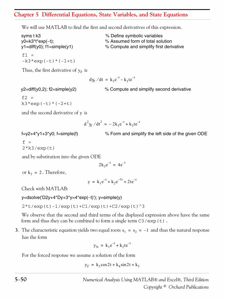
Chapter 5 Differential Equations, State Variables, and State Equations
5−50 Numerical Analysis Using MATLAB® and Excel®, Third EditionCopyright © Orchard Publications
We will use MATLAB to find the first and second derivatives of this expression.
syms t k3 % Define symbolic variablesy0=k3*t*exp(−t); % Assumed form of total solutiony1=diff(y0); f1=simple(y1) % Compute and simplify first derivative
f1 =-k3*exp(-t)*(-1+t)
Thus, the first derivative of is
y2=diff(y0,2); f2=simple(y2) % Compute and simplify second derivative
f2 =k3*exp(-t)*(-2+t)
and the second derivative of is
f=y2+4*y1+3*y0; f=simple(f) % Form and simplify the left side of the given ODE
f =2*k3/exp(t)
and by substitution into the given ODE
or . Therefore,
Check with MATLAB:
y=dsolve('D2y+4*Dy+3*y=4*exp(−t)'); y=simple(y)
2*t/exp(t)-1/exp(t)+C1/exp(t)+C2/exp(t)^3
We observe that the second and third terms of the displayed expression above have the sameform and thus they can be combined to form a single term C3/exp(t).
3. The characteristic equation yields two equal roots and thus the natural responsehas the form
For the forced response we assume a solution of the form
yF
dyF dt⁄ k3e t– k3te t––=
y
d 2yF dt2⁄ 2k3e t–– k3te t–+=
2k3e t– 4e t–=
k3 2=
y k1e t– k2e 3t– 2te t–+ +=
s1 s2 1–= =
yN k1e t– k2te t–+=
yF k3 2t k4 2t k5+sin+cos=
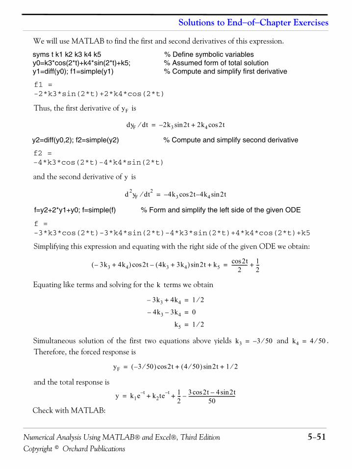
Numerical Analysis Using MATLAB® and Excel®, Third Edition 5−51Copyright © Orchard Publications
Solutions to End−of−Chapter Exercises
We will use MATLAB to find the first and second derivatives of this expression.
syms t k1 k2 k3 k4 k5 % Define symbolic variablesy0=k3*cos(2*t)+k4*sin(2*t)+k5; % Assumed form of total solutiony1=diff(y0); f1=simple(y1) % Compute and simplify first derivative
f1 =-2*k3*sin(2*t)+2*k4*cos(2*t)
Thus, the first derivative of is
y2=diff(y0,2); f2=simple(y2) % Compute and simplify second derivative
f2 =-4*k3*cos(2*t)-4*k4*sin(2*t)
and the second derivative of is
f=y2+2*y1+y0; f=simple(f) % Form and simplify the left side of the given ODE
f =-3*k3*cos(2*t)-3*k4*sin(2*t)-4*k3*sin(2*t)+4*k4*cos(2*t)+k5
Simplifying this expression and equating with the right side of the given ODE we obtain:
Equating like terms and solving for the terms we obtain
Simultaneous solution of the first two equations above yields and .Therefore, the forced response is
and the total response is
Check with MATLAB:
yF
dyF dt⁄ 2k– 3 2tsin 2k4 2tcos+=
y
d 2yF dt2⁄ 4k3 2tcos– 4k4– 2tsin=
3k3– 4k4+( ) 2tcos 4k3 3k4+( ) 2t k5+sin– 2tcos2
------------- 12---+=
k
3k3– 4k4+ 1 2⁄=
4k3– 3k4– 0=
k5 1 2⁄=
k3 3– 50⁄= k4 4 50⁄=
yF 3– 50⁄( ) 2t 4 50⁄( ) 2t 1 2⁄+sin+cos=
y k1e t– k2te t– 12--- 3 2tcos 4 2tsin–
50---------------------------------------–+ +=
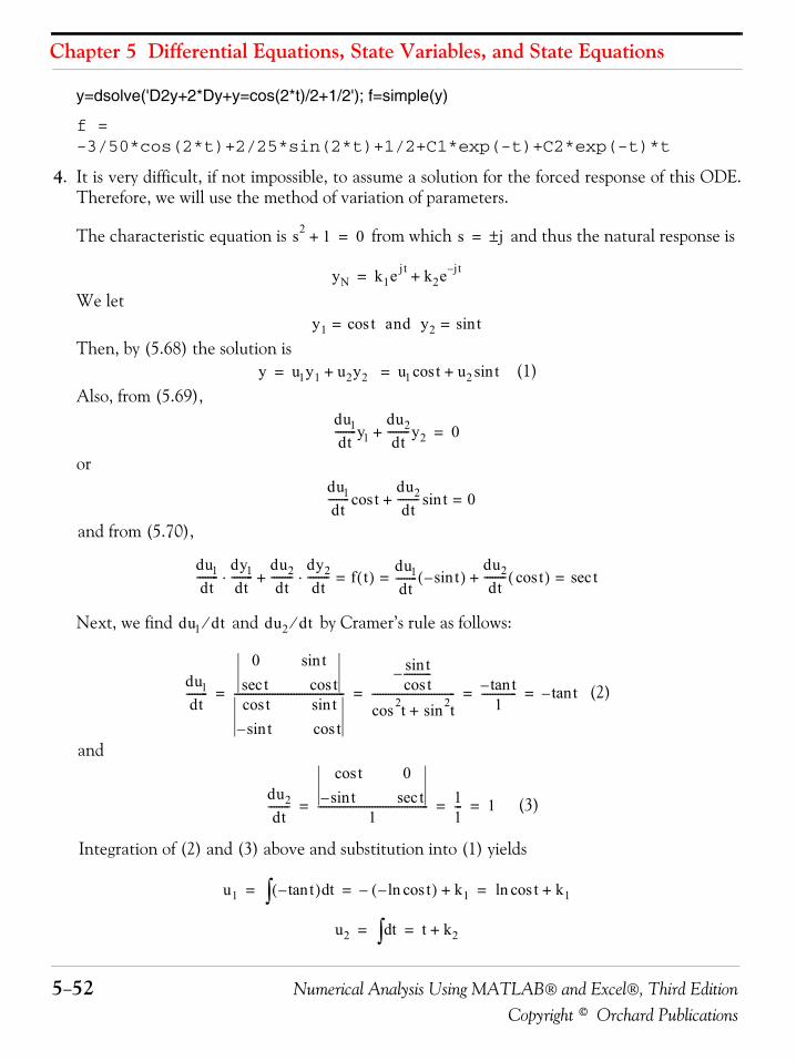
Chapter 5 Differential Equations, State Variables, and State Equations
5−52 Numerical Analysis Using MATLAB® and Excel®, Third EditionCopyright © Orchard Publications
y=dsolve('D2y+2*Dy+y=cos(2*t)/2+1/2'); f=simple(y)
f =-3/50*cos(2*t)+2/25*sin(2*t)+1/2+C1*exp(-t)+C2*exp(-t)*t
4. It is very difficult, if not impossible, to assume a solution for the forced response of this ODE.Therefore, we will use the method of variation of parameters.
The characteristic equation is from which and thus the natural response is
We let
Then, by (5.68) the solution is (1)
Also, from (5.69),
or
and from (5.70),
Next, we find and by Cramer’s rule as follows:
(2)
and
(3)
Integration of (2) and (3) above and substitution into (1) yields
s2 1+ 0= s j±=
yN k1e jt k2e j– t+=
y1 tcos= and y2 tsin=
y u1y1 u2y2 + u1 tcos u2 tsin += =
du1dt
--------y1du2dt
--------y2+ 0=
du1dt
-------- tcosdu2dt
-------- tsin+ 0=
du1dt
--------dy1dt
--------⋅du2dt
--------dy2dt
--------⋅+ f t( )du1dt
--------= = tsin–( )du2dt
-------- tcos( )+ tsec=
du1 dt⁄ du2 dt⁄
du1dt
--------
0 tsintsec tcostcos tsintsin– tcos
-----------------------------------------
tsintcos
----------–
t2cos t2sin+------------------------------- ttan–
1------------- ttan–= = = =
du2dt
--------
tcos 0tsin– tsec
1----------------------------------------- 1
1--- 1= = =
u1 ttan–( ) td∫ tcosln–( )– k1+ tcosln k1+= = =
u2 td∫ t k2+= =
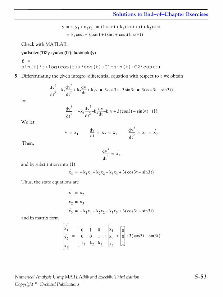
Numerical Analysis Using MATLAB® and Excel®, Third Edition 5−53Copyright © Orchard Publications
Solutions to End−of−Chapter Exercises
Check with MATLAB:
y=dsolve('D2y+y=sec(t)'); f=simple(y)
f =sin(t)*t+log(cos(t))*cos(t)+C1*sin(t)+C2*cos(t)
5. Differentiating the given integro−differential equation with respect to we obtain
or
(1)
We let
Then,
and by substitution into (1)
Thus, the state equations are
and in matrix form
y u1y1 u2y2 + tcosln k1+( ) tcos t k2+( ) tsin+= =
k1 tcos k2 tsin t tsin t tcosln( )cos+ + +=
t
dv3
dt3-------- k3
dv2
dt2-------- k2
dvdt------ k1v+ + + 3 3t 3 3tsin–cos 3 3t 3tsin–cos( )= =
dv3
dt3-------- k3
dv2
dt2--------–= k2– dv
dt------ k1– v 3 3t 3tsin–cos( )+
v x1= dvdt------ x2 x1
·= = dv2
dt2-------- x3 x2
·= =
dv3
dt3-------- x3
·=
x3· k1x1– k2x2– k3x3– 3 3t 3tsin–cos( )+=
x1· x2=
x2· x3=
x3· k1x1– k2x2– k3x3– 3 3t 3tsin–cos( )+=
x1·
x2·
x3·
0 1 00 0 1k1– k2– k– 3
x1
x2
x3
⋅001
3 3t 3tsin–cos( )⋅+=
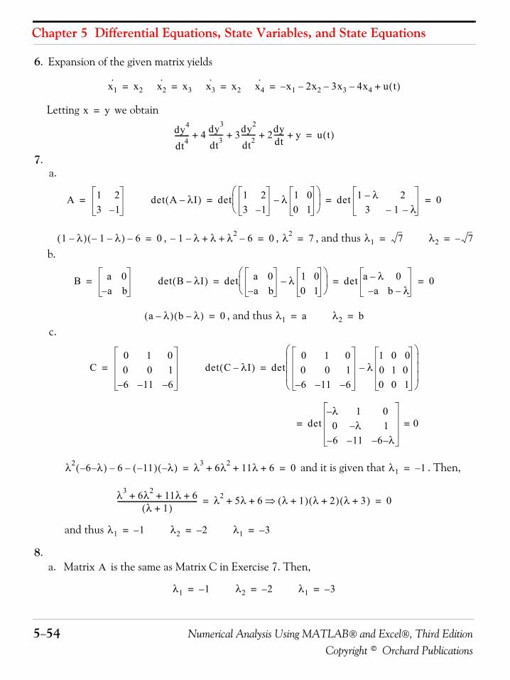
Chapter 5 Differential Equations, State Variables, and State Equations
5−54 Numerical Analysis Using MATLAB® and Excel®, Third EditionCopyright © Orchard Publications
6. Expansion of the given matrix yields
Letting we obtain
7.a.
, , , and thus b.
, and thus c.
and it is given that . Then,
and thus
8.a. Matrix is the same as Matrix C in Exercise 7. Then,
x1· x2= x2
· x3= x3· x2= x4
· x– 1 2x2– 3x3– 4x4– u t( )+=
x y=
dy4
dt4-------- 4 dy3
dt3-------- 3dy2
dt2-------- 2dy
dt------ y+ + ++ u t( )=
A 1 23 1–
= det A λI–( ) det 1 23 1–
λ 1 00 1
–⎝ ⎠⎜ ⎟⎛ ⎞
det 1 λ– 23 1– λ–
0= = =
1 λ–( ) 1– λ–( ) 6– 0= 1– λ– λ λ2 6–+ + 0= λ2 7= λ1 7= λ2 7–=
B a 0a– b
= det B λI–( ) det a 0a– b
λ 1 00 1
–⎝ ⎠⎜ ⎟⎛ ⎞
det a λ– 0a– b λ–
0= = =
a λ–( ) b λ–( ) 0= λ1 a= λ2 b=
C0 1 00 0 16– 11– 6–
= det C λI–( ) det0 1 00 0 16– 11– 6–
λ1 0 00 1 00 0 1
–
⎝ ⎠⎜ ⎟⎜ ⎟⎜ ⎟⎛ ⎞
=
detλ– 1 00 λ– 16– 11– 6 λ––
0==
λ2 6– λ–( ) 6– 11–( ) λ–( )– λ3 6λ2 11λ 6+ + + 0= = λ1 1–=
λ3 6λ2 11λ 6+ + +λ 1+( )
---------------------------------------------- λ2 5λ 6+ + λ 1+( ) λ 2+( ) λ 3+( )⇒ 0= =
λ1 1–= λ2 2–= λ1 3–=
A
λ1 1–= λ2 2–= λ1 3–=
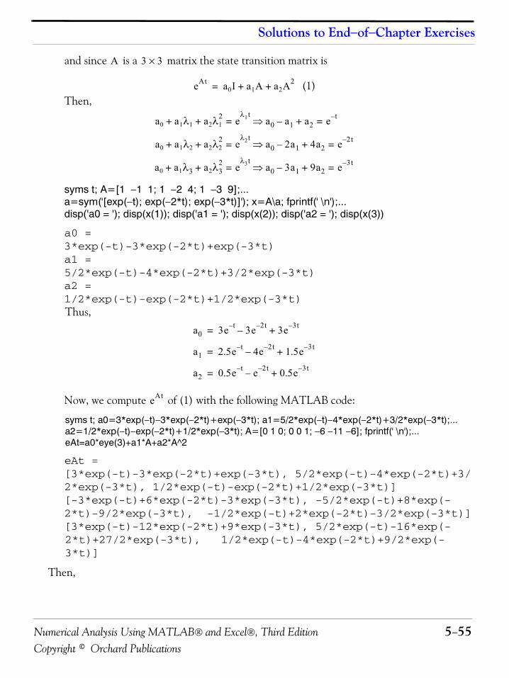
Numerical Analysis Using MATLAB® and Excel®, Third Edition 5−55Copyright © Orchard Publications
Solutions to End−of−Chapter Exercises
and since is a matrix the state transition matrix is
(1)Then,
syms t; A=[1 −1 1; 1 −2 4; 1 −3 9];...a=sym('[exp(−t); exp(−2*t); exp(−3*t)]'); x=A\a; fprintf(' \n');...disp('a0 = '); disp(x(1)); disp('a1 = '); disp(x(2)); disp('a2 = '); disp(x(3))
a0 = 3*exp(-t)-3*exp(-2*t)+exp(-3*t)a1 = 5/2*exp(-t)-4*exp(-2*t)+3/2*exp(-3*t)a2 = 1/2*exp(-t)-exp(-2*t)+1/2*exp(-3*t)Thus,
Now, we compute of (1) with the following MATLAB code:
syms t; a0=3*exp(−t)−3*exp(−2*t)+exp(−3*t); a1=5/2*exp(−t)−4*exp(−2*t)+3/2*exp(−3*t);...a2=1/2*exp(−t)−exp(−2*t)+1/2*exp(−3*t); A=[0 1 0; 0 0 1; −6 −11 −6]; fprintf(' \n');...eAt=a0*eye(3)+a1*A+a2*A^2
eAt =[3*exp(-t)-3*exp(-2*t)+exp(-3*t), 5/2*exp(-t)-4*exp(-2*t)+3/2*exp(-3*t), 1/2*exp(-t)-exp(-2*t)+1/2*exp(-3*t)][-3*exp(-t)+6*exp(-2*t)-3*exp(-3*t), -5/2*exp(-t)+8*exp(-2*t)-9/2*exp(-3*t), -1/2*exp(-t)+2*exp(-2*t)-3/2*exp(-3*t)][3*exp(-t)-12*exp(-2*t)+9*exp(-3*t), 5/2*exp(-t)-16*exp(-2*t)+27/2*exp(-3*t), 1/2*exp(-t)-4*exp(-2*t)+9/2*exp(-3*t)]
Then,
A 3 3×
eAt a0I a1A a2A2+ +=
a0 a1λ1 a2λ12+ + e
λ1t= a0 a1– a2+ e t–=⇒
a0 a1λ2 a2λ22+ + e
λ2t= a0 2a1– 4a2+ e 2t–=⇒
a0 a1λ3 a2λ32+ + e
λ3t= a0 3a1– 9a2+ e 3t–=⇒
a0 3e t– 3e 2t–– 3e 3t–+=
a1 2.5e t– 4e 2t–– 1.5e 3t–+=
a2 0.5e t– e 2t–– 0.5e 3t–+=
eAt
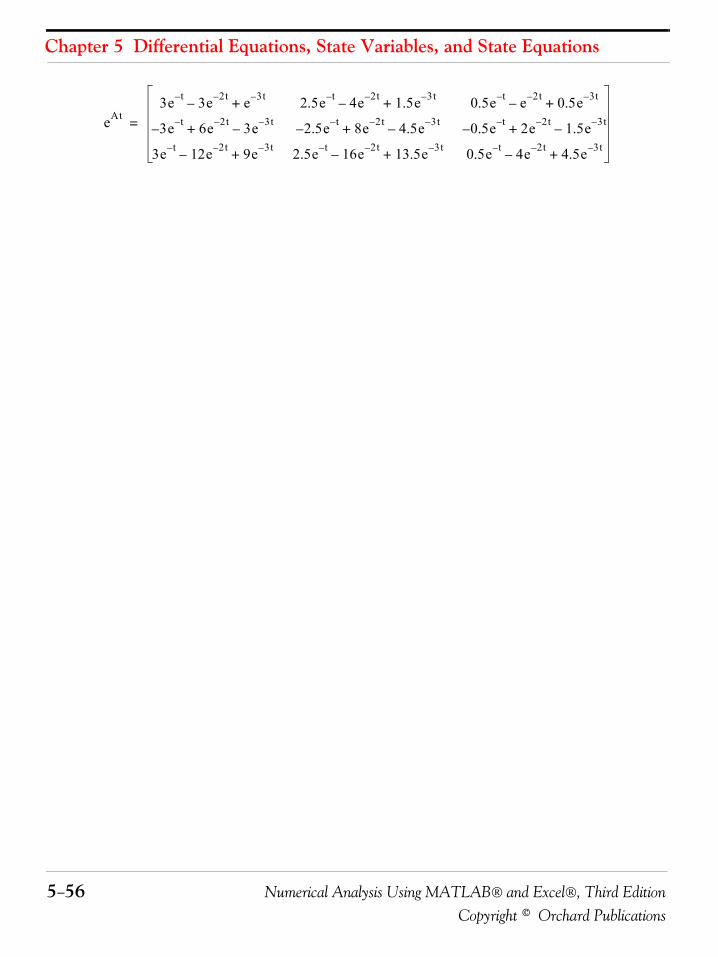
Chapter 5 Differential Equations, State Variables, and State Equations
5−56 Numerical Analysis Using MATLAB® and Excel®, Third EditionCopyright © Orchard Publications
eAt3e t– 3e 2t–– e 3t–+ 2.5e t– 4e 2t–– 1.5e 3t–+ 0.5e t– e 2t–– 0.5e 3t–+
3– e t– 6e 2t– 3e 3t––+ 2.5– e t– 8e 2t– 4.5e 3t––+ 0.5– e t– 2e 2t– 1.5e 3t––+
3e t– 12e 2t–– 9e 3t–+ 2.5e t– 16e 2t–– 13.5e 3t–+ 0.5e t– 4e 2t–– 4.5e 3t–+
=
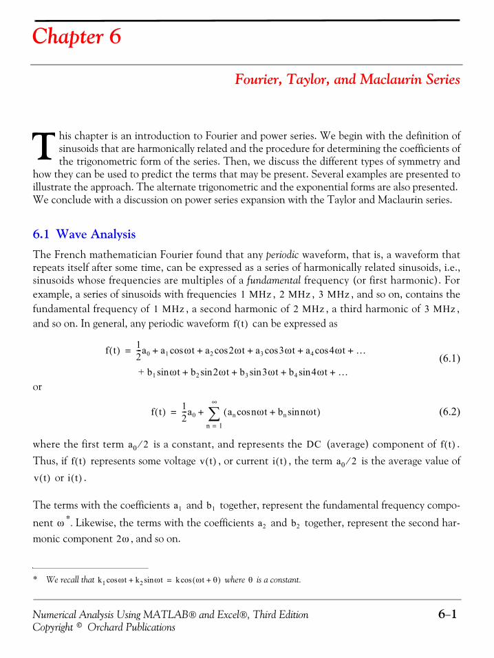
Numerical Analysis Using MATLAB® and Excel®, Third Edition 6−1Copyright © Orchard Publications
Chapter 6
Fourier, Taylor, and Maclaurin Series
his chapter is an introduction to Fourier and power series. We begin with the definition ofsinusoids that are harmonically related and the procedure for determining the coefficients ofthe trigonometric form of the series. Then, we discuss the different types of symmetry and
how they can be used to predict the terms that may be present. Several examples are presented toillustrate the approach. The alternate trigonometric and the exponential forms are also presented. We conclude with a discussion on power series expansion with the Taylor and Maclaurin series.
6.1 Wave AnalysisThe French mathematician Fourier found that any periodic waveform, that is, a waveform thatrepeats itself after some time, can be expressed as a series of harmonically related sinusoids, i.e.,sinusoids whose frequencies are multiples of a fundamental frequency (or first harmonic). Forexample, a series of sinusoids with frequencies , , , and so on, contains thefundamental frequency of , a second harmonic of , a third harmonic of ,and so on. In general, any periodic waveform can be expressed as
(6.1)
or
(6.2)
where the first term is a constant, and represents the (average) component of .Thus, if represents some voltage , or current , the term is the average value of
or .
The terms with the coefficients and together, represent the fundamental frequency compo-
nent *. Likewise, the terms with the coefficients and together, represent the second har-monic component , and so on.
* We recall that where is a constant.
T
1 MHz 2 MHz 3 MHz1 MHz 2 MHz 3 MHz
f t( )
f t( ) 12---a0 a1 ωtcos a2 2ωtcos a3 3ωt a4 4ωtcos+cos …+ + + +=
+ b1 ωtsin b2 2ωtsin b3 3ωt b4 4ωtsin+sin …+ + +
f t( ) 12---a0 an nωtcos bn nωtsin+( )
n 1=
∞
∑+=
a0 2⁄ DC f t( )
f t( ) v t( ) i t( ) a0 2⁄
v t( ) i t( )
a1 b1
ω a2 b2
k1 ωtcos k2 ωtsin+ k ωt θ+( )cos= θ
2ω
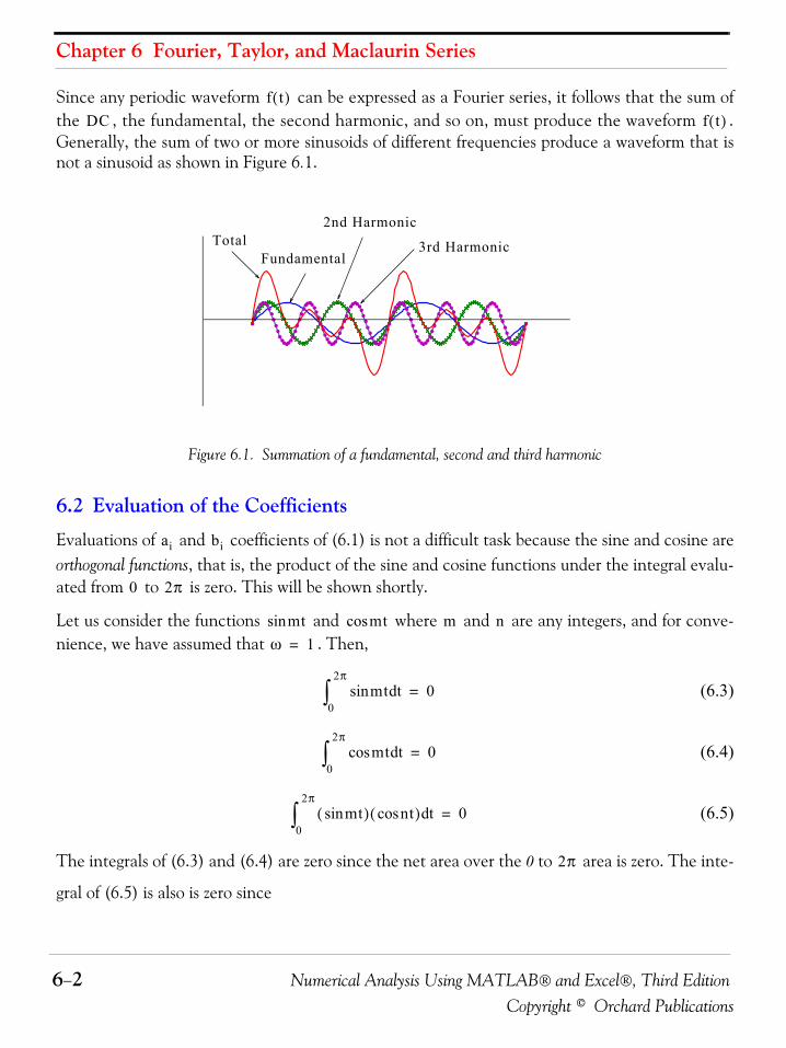
Chapter 6 Fourier, Taylor, and Maclaurin Series
6−2 Numerical Analysis Using MATLAB® and Excel®, Third EditionCopyright © Orchard Publications
Since any periodic waveform can be expressed as a Fourier series, it follows that the sum ofthe , the fundamental, the second harmonic, and so on, must produce the waveform .Generally, the sum of two or more sinusoids of different frequencies produce a waveform that isnot a sinusoid as shown in Figure 6.1.
Figure 6.1. Summation of a fundamental, second and third harmonic
6.2 Evaluation of the Coefficients
Evaluations of and coefficients of (6.1) is not a difficult task because the sine and cosine areorthogonal functions, that is, the product of the sine and cosine functions under the integral evalu-ated from to is zero. This will be shown shortly.
Let us consider the functions and where and are any integers, and for conve-nience, we have assumed that . Then,
(6.3)
(6.4)
(6.5)
The integrals of (6.3) and (6.4) are zero since the net area over the 0 to area is zero. The inte-
gral of (6.5) is also is zero since
f t( )DC f t( )
0 2 4 6 8 10 12-3
-2
-1
0
1
2
3
TotalFundamental
2nd Harmonic
3rd Harmonic
ai bi
0 2π
mtsin mcos t m nω 1=
mtsin td0
2π
∫ 0=
mcos t td0
2π
∫ 0=
mtsin( ) ntcos( )0
2π
∫ td 0=
2π
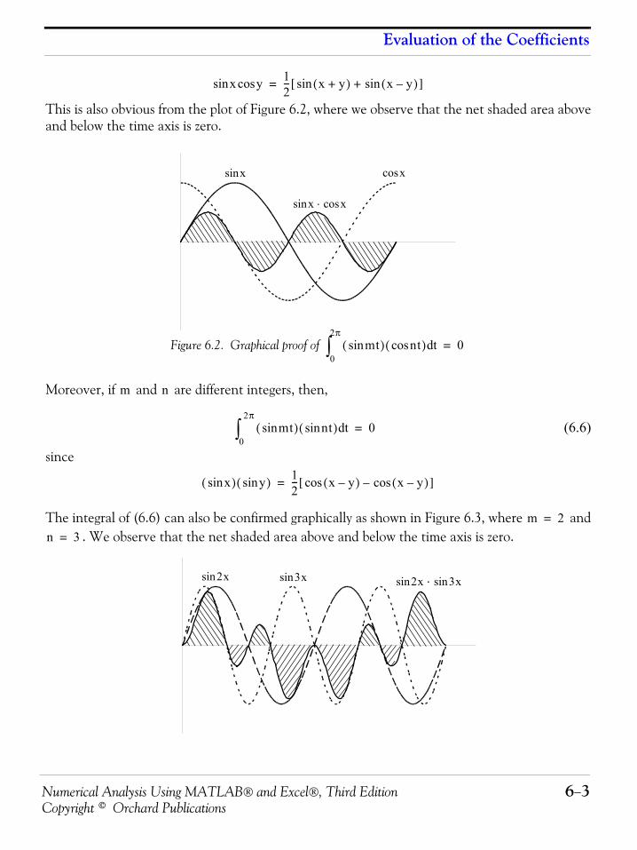
Numerical Analysis Using MATLAB® and Excel®, Third Edition 6−3Copyright © Orchard Publications
Evaluation of the Coefficients
This is also obvious from the plot of Figure 6.2, where we observe that the net shaded area aboveand below the time axis is zero.
Figure 6.2. Graphical proof of
Moreover, if and are different integers, then,
(6.6)
since
The integral of (6.6) can also be confirmed graphically as shown in Figure 6.3, where and. We observe that the net shaded area above and below the time axis is zero.
x ycossin 12--- x y+( )sin x y–( )sin+[ ]=
xsin xcos
xsin xcos⋅
mtsin( ) ntcos( )0
2π
∫ td 0=
m n
mtsin( ) ntsin( ) td0
2π
∫ 0=
xsin( ) ysin( ) 12--- x y–( )cos x y–( )cos–[ ]=
m 2=
n 3=
2xsin 3xsin 2xsin 3xsin⋅
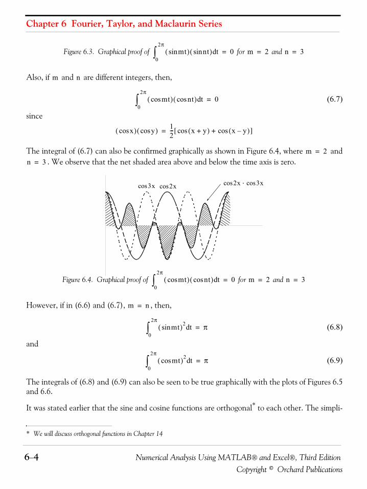
Chapter 6 Fourier, Taylor, and Maclaurin Series
6−4 Numerical Analysis Using MATLAB® and Excel®, Third EditionCopyright © Orchard Publications
Figure 6.3. Graphical proof of for and
Also, if and are different integers, then,
(6.7)
since
The integral of (6.7) can also be confirmed graphically as shown in Figure 6.4, where and. We observe that the net shaded area above and below the time axis is zero.
Figure 6.4. Graphical proof of for and
However, if in (6.6) and (6.7), , then,
(6.8)
and
(6.9)
The integrals of (6.8) and (6.9) can also be seen to be true graphically with the plots of Figures 6.5and 6.6.
It was stated earlier that the sine and cosine functions are orthogonal* to each other. The simpli-
* We will discuss orthogonal functions in Chapter 14
mtsin( ) ntsin( ) td0
2π
∫ 0= m 2= n 3=
m n
mcos t( ) ntcos( ) td0
2π
∫ 0=
xcos( ) ycos( ) 12--- x y+( )cos x y–( )cos+[ ]=
m 2=
n 3=
3xcos 2xcos 2xcos 3xcos⋅
mcos t( ) ntcos( ) td0
2π
∫ 0= m 2= n 3=
m n=
mtsin( )2 td0
2π
∫ π=
mcos t( )2 td0
2π
∫ π=
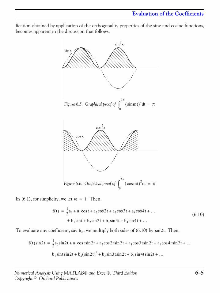
Numerical Analysis Using MATLAB® and Excel®, Third Edition 6−5Copyright © Orchard Publications
Evaluation of the Coefficients
fication obtained by application of the orthogonality properties of the sine and cosine functions,becomes apparent in the discussion that follows.
Figure 6.5. Graphical proof of
Figure 6.6. Graphical proof of
In (6.1), for simplicity, we let . Then,
(6.10)
To evaluate any coefficient, say , we multiply both sides of (6.10) by . Then,
xsinx2sin
mtsin( )2 td0
2π
∫ π=
xcos
x2cos
mcos t( )2 td0
2π
∫ π=
ω 1=
f t( ) 12---a0 a1 tcos a2 2tcos a3 3t a4 4tcos+cos …+ + + +=
+ b1 tsin b2 2tsin b3 3t b4 4tsin+sin …+ + +
b2 2tsin
f t( ) 2tsin 12---a0 2tsin a1 t 2tsincos a2 2t 2tsincos a3 3t 2tsin a4 4t 2tsincos+cos …+ + + +=
b1 t 2tsinsin b2 2tsin( )2 b3 3t 2tsin b4 4t 2tsinsin+sin …+ + +
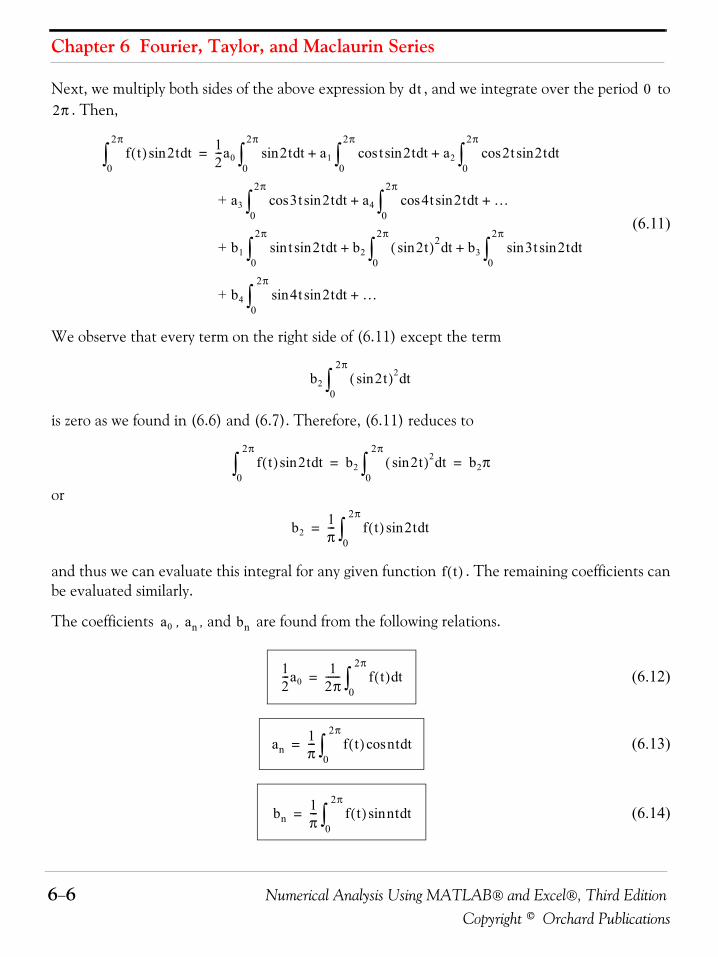
Chapter 6 Fourier, Taylor, and Maclaurin Series
6−6 Numerical Analysis Using MATLAB® and Excel®, Third EditionCopyright © Orchard Publications
Next, we multiply both sides of the above expression by , and we integrate over the period to. Then,
(6.11)
We observe that every term on the right side of (6.11) except the term
is zero as we found in (6.6) and (6.7). Therefore, (6.11) reduces to
or
and thus we can evaluate this integral for any given function . The remaining coefficients canbe evaluated similarly.
The coefficients , , and are found from the following relations.
(6.12)
(6.13)
(6.14)
dt 02π
f t( ) 2tsin td0
2π
∫12---a0 2tsin td
0
2π
∫ a1 t 2tsincos td0
2π
∫ a2 2t 2tsincos td0
2π
∫+ +=
+ a3 3t 2tsincos td0
2π
∫ a4 4t 2tsincos td0
2π
∫ …+ +
+ b1 tsin 2tsin td0
2π
∫ b2 2tsin( )2 td0
2π
∫ b3 3tsin 2tsin td0
2π
∫+ +
+ b4 4tsin 2tsin td0
2π
∫ …+
b2 2tsin( )2 td0
2π
∫
f t( ) 2tsin td0
2π
∫ b2 2tsin( )2 td0
2π
∫ b2π= =
b21π--- f t( ) 2tsin td
0
2π
∫=
f t( )
a0 an bn
12---a0
12π------ f t( ) td
0
2π
∫=
an1π--- f t( ) nt tdcos
0
2π
∫=
bn1π--- f t( ) nt tdsin
0
2π
∫=
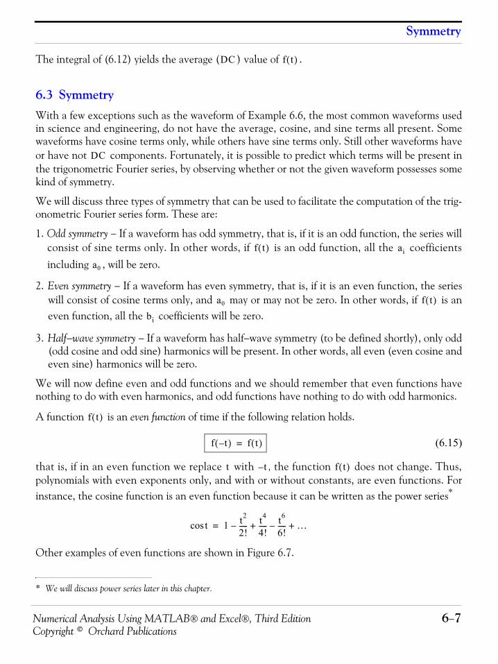
Numerical Analysis Using MATLAB® and Excel®, Third Edition 6−7Copyright © Orchard Publications
Symmetry
The integral of (6.12) yields the average ( ) value of .
6.3 SymmetryWith a few exceptions such as the waveform of Example 6.6, the most common waveforms usedin science and engineering, do not have the average, cosine, and sine terms all present. Somewaveforms have cosine terms only, while others have sine terms only. Still other waveforms haveor have not components. Fortunately, it is possible to predict which terms will be present inthe trigonometric Fourier series, by observing whether or not the given waveform possesses somekind of symmetry.
We will discuss three types of symmetry that can be used to facilitate the computation of the trig-onometric Fourier series form. These are:
1. Odd symmetry − If a waveform has odd symmetry, that is, if it is an odd function, the series willconsist of sine terms only. In other words, if is an odd function, all the coefficientsincluding , will be zero.
2. Even symmetry − If a waveform has even symmetry, that is, if it is an even function, the serieswill consist of cosine terms only, and may or may not be zero. In other words, if is aneven function, all the coefficients will be zero.
3. Half−wave symmetry − If a waveform has half−wave symmetry (to be defined shortly), only odd(odd cosine and odd sine) harmonics will be present. In other words, all even (even cosine andeven sine) harmonics will be zero.
We will now define even and odd functions and we should remember that even functions havenothing to do with even harmonics, and odd functions have nothing to do with odd harmonics.
A function is an even function of time if the following relation holds.
(6.15)
that is, if in an even function we replace with , the function does not change. Thus,polynomials with even exponents only, and with or without constants, are even functions. Forinstance, the cosine function is an even function because it can be written as the power series*
Other examples of even functions are shown in Figure 6.7.
* We will discuss power series later in this chapter.
DC f t( )
DC
f t( ) ai
a0
a0 f t( )bi
f t( )
f t–( ) f t( )=
t t– f t( )
tcos 1 t2
2!----- t4
4!-----+– t6
6!-----– …+=
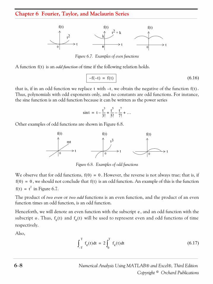
Chapter 6 Fourier, Taylor, and Maclaurin Series
6−8 Numerical Analysis Using MATLAB® and Excel®, Third EditionCopyright © Orchard Publications
Figure 6.7. Examples of even functions
A function is an odd function of time if the following relation holds.
(6.16)
that is, if in an odd function we replace with , we obtain the negative of the function .Thus, polynomials with odd exponents only, and no constants are odd functions. For instance,the sine function is an odd function because it can be written as the power series
Other examples of odd functions are shown in Figure 6.8.
Figure 6.8. Examples of odd functions
We observe that for odd functions, . However, the reverse is not always true; that is, if, we should not conclude that is an odd function. An example of this is the function
in Figure 6.7.
The product of two even or two odd functions is an even function, and the product of an evenfunction times an odd function, is an odd function.
Henceforth, we will denote an even function with the subscript , and an odd function with thesubscript . Thus, and will be used to represent even and odd functions of timerespectively.
Also,
(6.17)
t
f(t)
t
f(t)
t
f(t)
k
0 0 0
t2t2 k+
f t( )
f– t–( ) f t( )=
t t– f t( )
tsin t t3
3!----- t5
5!-----+– t7
7!-----– …+=
t
f(t)
mt
t
f(t)
t
f(t)
0 0 0
t3
f 0( ) 0=
f 0( ) 0= f t( )
f t( ) t2=
eo fe t( ) fo t( )
fe t( ) tdT–
T
∫ 2 fe t( ) td0
T
∫=
Numerical Analysis Using MATLAB® and Excel®, Third Edition 6−9Copyright © Orchard Publications
Symmetry
and
(6.18)
A function that is neither even nor odd can be expressed as
(6.19)
or as
(6.20)
By addition of (6.16) with (6.17), we get
(6.21)
that is, any function of time can be expressed as the sum of an even and an odd function.
To understand half−wave symmetry, we recall that any periodic function with period , isexpressed as
(6.22)
that is, the function with value at any time , will have the same value again at a later time.
A periodic waveform with period , has half−wave symmetry if
(6.23)
that is, the shape of the negative half−cycle of the waveform is the same as that of the positivehalf−cycle, but inverted.
We will test the waveforms of Figures 6.9 through 6.13 for any of the three types of symmetry.
1. Square waveform
For the waveform of Figure 6.9, the average value over one period is zero, and therefore,. It is also an odd function and has half−wave symmetry since and
.
fo t( ) tdT–
T
∫ 0=
f t( )
fe t( ) 12--- f t( ) f t–( )+[ ]=
fo t( ) 12--- f t( ) f– t–( )[ ]=
f t( ) fe t( ) fo t( )+=
T
f t( ) f t T+( )=
f t( ) tt T+
T
f– t T 2⁄+( ) f t( )=
Ta0 0= f t–( )– f t( )=
f t T 2⁄+( )– f t( )=
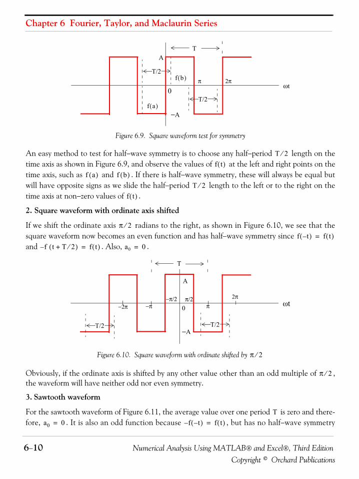
Chapter 6 Fourier, Taylor, and Maclaurin Series
6−10 Numerical Analysis Using MATLAB® and Excel®, Third EditionCopyright © Orchard Publications
Figure 6.9. Square waveform test for symmetry
An easy method to test for half−wave symmetry is to choose any half−period length on thetime axis as shown in Figure 6.9, and observe the values of at the left and right points on thetime axis, such as and . If there is half−wave symmetry, these will always be equal butwill have opposite signs as we slide the half−period length to the left or to the right on thetime axis at non−zero values of .
2. Square waveform with ordinate axis shifted
If we shift the ordinate axis radians to the right, as shown in Figure 6.10, we see that thesquare waveform now becomes an even function and has half−wave symmetry since and . Also, .
Figure 6.10. Square waveform with ordinate shifted by
Obviously, if the ordinate axis is shifted by any other value other than an odd multiple of ,the waveform will have neither odd nor even symmetry.
3. Sawtooth waveform
For the sawtooth waveform of Figure 6.11, the average value over one period is zero and there-fore, . It is also an odd function because , but has no half−wave symmetry
0π 2π
T
ωt
T/2
T/2
A
−Af a( )
f b( )
T 2⁄f t( )
f a( ) f b( )T 2⁄
f t( )
π 2⁄f t–( ) f t( )=
f t T 2⁄+( )– f t( )= a0 0=
0π/2 2π
T
ωt
T/2 T/2
A
−A
−π/2π−π−2π
π 2⁄
π 2⁄
Ta0 0= f t–( )– f t( )=
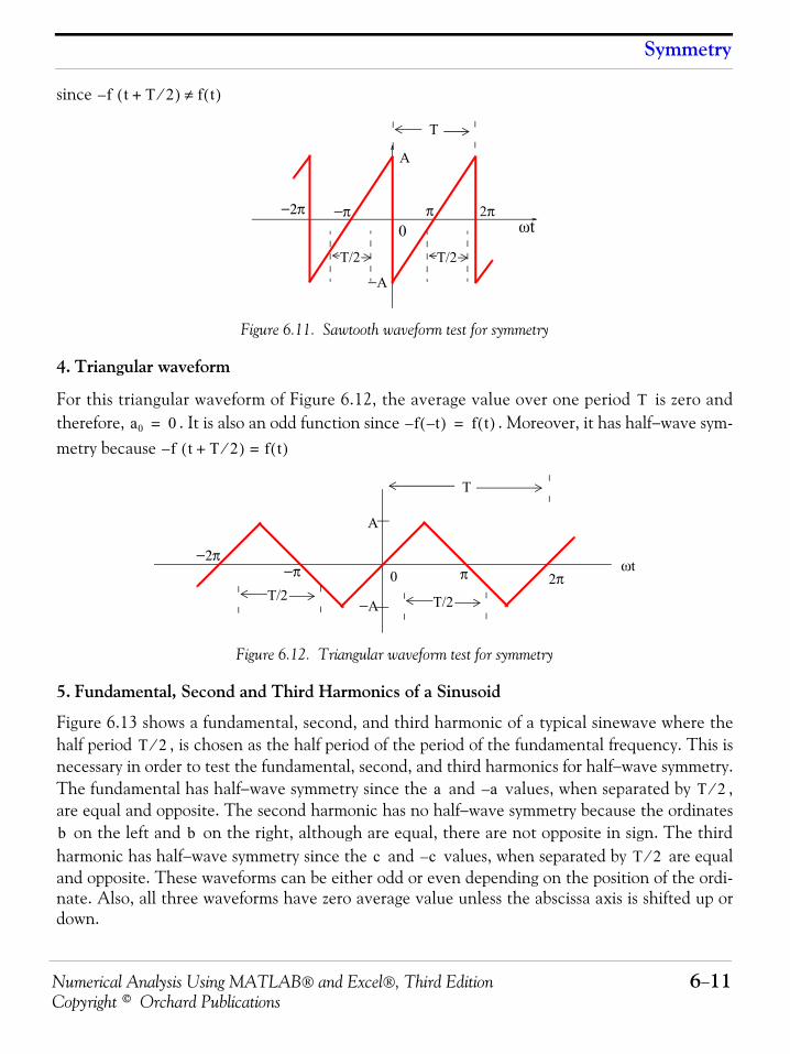
Numerical Analysis Using MATLAB® and Excel®, Third Edition 6−11Copyright © Orchard Publications
Symmetry
since
Figure 6.11. Sawtooth waveform test for symmetry
4. Triangular waveform
For this triangular waveform of Figure 6.12, the average value over one period is zero andtherefore, . It is also an odd function since . Moreover, it has half−wave sym-metry because
Figure 6.12. Triangular waveform test for symmetry
5. Fundamental, Second and Third Harmonics of a Sinusoid
Figure 6.13 shows a fundamental, second, and third harmonic of a typical sinewave where thehalf period , is chosen as the half period of the period of the fundamental frequency. This isnecessary in order to test the fundamental, second, and third harmonics for half−wave symmetry.The fundamental has half−wave symmetry since the and values, when separated by ,are equal and opposite. The second harmonic has no half−wave symmetry because the ordinates
on the left and on the right, although are equal, there are not opposite in sign. The thirdharmonic has half−wave symmetry since the and values, when separated by are equaland opposite. These waveforms can be either odd or even depending on the position of the ordi-nate. Also, all three waveforms have zero average value unless the abscissa axis is shifted up ordown.
f t T 2⁄+( ) f t( )≠–
02π
T
ωt
T/2
A
−A
π−π−2π
T/2
Ta0 0= f t–( )– f t( )=
f t T 2⁄+( ) f t( )=–
0 2π
T
ωt
A
−A
π−π−2π
T/2 T/2
T 2⁄
a a– T 2⁄
b bc c– T 2⁄
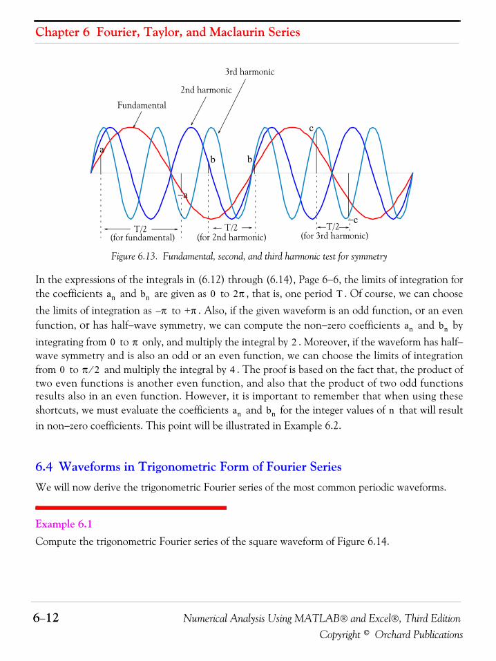
Chapter 6 Fourier, Taylor, and Maclaurin Series
6−12 Numerical Analysis Using MATLAB® and Excel®, Third EditionCopyright © Orchard Publications
Figure 6.13. Fundamental, second, and third harmonic test for symmetry
In the expressions of the integrals in (6.12) through (6.14), Page 6−6, the limits of integration forthe coefficients and are given as to , that is, one period . Of course, we can choosethe limits of integration as to . Also, if the given waveform is an odd function, or an evenfunction, or has half−wave symmetry, we can compute the non−zero coefficients and byintegrating from to only, and multiply the integral by . Moreover, if the waveform has half−wave symmetry and is also an odd or an even function, we can choose the limits of integrationfrom to and multiply the integral by . The proof is based on the fact that, the product oftwo even functions is another even function, and also that the product of two odd functionsresults also in an even function. However, it is important to remember that when using theseshortcuts, we must evaluate the coefficients and for the integer values of that will resultin non−zero coefficients. This point will be illustrated in Example 6.2.
6.4 Waveforms in Trigonometric Form of Fourier Series We will now derive the trigonometric Fourier series of the most common periodic waveforms.
Example 6.1 Compute the trigonometric Fourier series of the square waveform of Figure 6.14.
0 2 4 6 8 10 12-1
-0.5
0
0.5
1
a
−a
b b
−c
c
Fundamental
2nd harmonic
3rd harmonic
T/2(for fundamental) (for 2nd harmonic)
T/2 T/2(for 3rd harmonic)
an bn 0 2π T
π– +πan bn
0 π 2
0 π 2⁄ 4
an bn n
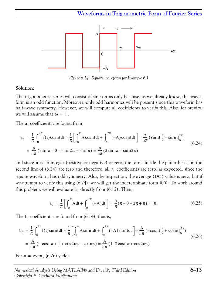
Numerical Analysis Using MATLAB® and Excel®, Third Edition 6−13Copyright © Orchard Publications
Waveforms in Trigonometric Form of Fourier Series
Figure 6.14. Square waveform for Example 6.1
Solution:
The trigonometric series will consist of sine terms only because, as we already know, this wave-form is an odd function. Moreover, only odd harmonics will be present since this waveform hashalf−wave symmetry. However, we will compute all coefficients to verify this. Also, for brevity,we will assume that .
The coefficients are found from
(6.24)
and since is an integer (positive or negative) or zero, the terms inside the parentheses on thesecond line of (6.24) are zero and therefore, all coefficients are zero, as expected, since thesquare waveform has odd symmetry. Also, by inspection, the average ( ) value is zero, but ifwe attempt to verify this using (6.24), we will get the indeterminate form . To work aroundthis problem, we will evaluate directly from (6.12). Then,
(6.25)
The coefficients are found from (6.14), that is,
(6.26)
For , (6.26) yields
0π 2π
T
ωt
A
−A
ω 1=
ai
an1π--- f t( ) ntcos td
0
2π
∫1π--- A ntcos td
0
π
∫ A–( ) ntcos tdπ
2π
∫+Anπ------ ntsin 0
π ntsin π2π–( )= ==
Anπ------ nπ 0– n2π nπsin+sin–sin( ) A
nπ------ 2 nπ n2πsin–sin( )==
nai
DC0 0⁄
a0
a01π--- A td
0
π
∫ A–( ) tdπ
2π
∫+ Aπ---- π 0– 2π– π+( ) 0= = =
bi
bn1π--- f t( ) ntsin td
0
2π
∫1π--- A ntsin td
0
π
∫ A–( ) ntsin tdπ
2π
∫+ Anπ------ ncos– t 0
π ntcos π2π+( )= ==
Anπ------ nπcos– 1 2nπ nπcos–cos+ +( ) A
nπ------ 1 2 nπcos– 2nπcos+( )==
n even=
Chapter 6 Fourier, Taylor, and Maclaurin Series
6−14 Numerical Analysis Using MATLAB® and Excel®, Third EditionCopyright © Orchard Publications
as expected, since the square waveform has half−wave symmetry.
For , (6.21) reduces to
and thus
and so on.
Therefore, the trigonometric Fourier series for the square waveform with odd symmetry is
(6.27)
It was stated above that, if the given waveform has half−wave symmetry, and it is also an odd oran even function, we can integrate from to , and multiply the integral by . We will applythis property to the following example.
Example 6.2 Compute the trigonometric Fourier series of the square waveform of Example 1 by integratingfrom to , and multiplying the result by .
Solution:
Since the waveform is an odd function and has half−wave symmetry, we are only concerned withthe odd coefficients. Then,
(6.28)
For , (6.28) becomes
bnAnπ------ 1 2– 1+( ) 0= =
n odd=
bnAnπ------ 1 2 1+ +( ) 4A
nπ-------= =
b14Aπ
-------=
b34A3π-------=
b54A5π-------=
f t( ) 4Aπ
------- ωt 13--- 3ωt 1
5--- 5ωtsin …+ +sin+sin⎝ ⎠
⎛ ⎞ 4Aπ
------- 1n--- nωtsin
n odd=∑= =
0 π 2⁄ 4
0 π 2⁄ 4
bn
bn 41π--- f t( ) ntsin td
0
π 2⁄
∫4Anπ------- ncos– t 0
π 2⁄( ) 4Anπ------- nπ
2---cos– 1+⎝ ⎠
⎛ ⎞= = =
n odd=
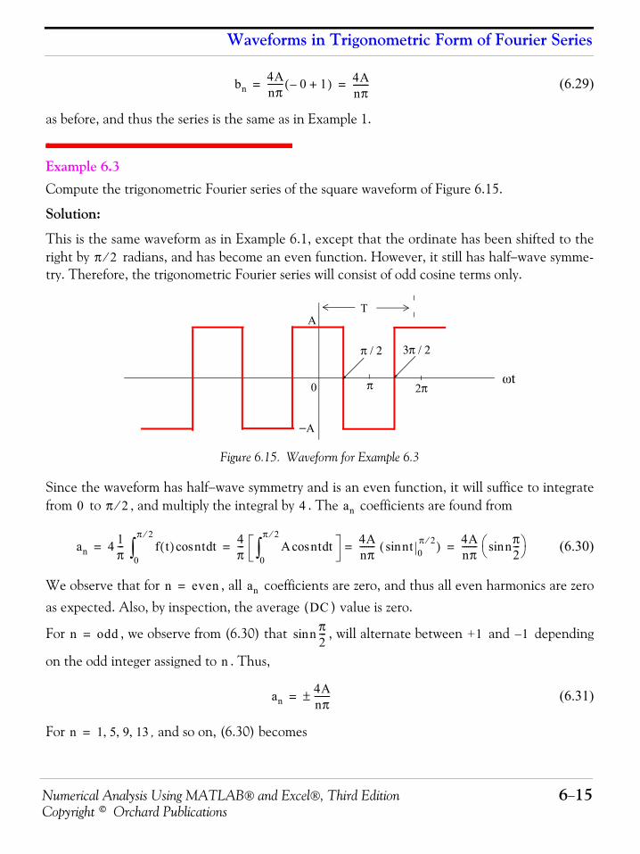
Numerical Analysis Using MATLAB® and Excel®, Third Edition 6−15Copyright © Orchard Publications
Waveforms in Trigonometric Form of Fourier Series
(6.29)
as before, and thus the series is the same as in Example 1.
Example 6.3 Compute the trigonometric Fourier series of the square waveform of Figure 6.15.
Solution:
This is the same waveform as in Example 6.1, except that the ordinate has been shifted to theright by radians, and has become an even function. However, it still has half−wave symme-try. Therefore, the trigonometric Fourier series will consist of odd cosine terms only.
Figure 6.15. Waveform for Example 6.3
Since the waveform has half−wave symmetry and is an even function, it will suffice to integratefrom to , and multiply the integral by . The coefficients are found from
(6.30)
We observe that for , all coefficients are zero, and thus all even harmonics are zeroas expected. Also, by inspection, the average ( ) value is zero.
For , we observe from (6.30) that , will alternate between and depending
on the odd integer assigned to . Thus,
(6.31)
For , and so on, (6.30) becomes
bn4Anπ------- 0– 1+( ) 4A
nπ-------= =
π 2⁄
0
π / 2
2π
T
ωt
A
−A
π
3π / 2
0 π 2⁄ 4 an
an 4 1π--- f t( ) ntcos td
0
π 2⁄
∫4π--- A ntcos td
0
π 2⁄
∫4Anπ------- ntsin 0
π 2⁄( ) 4Anπ------- nπ
2---sin⎝ ⎠
⎛ ⎞= = = =
n even= an
DC
n odd= n π2---sin +1 1–
n
an4Anπ-------±=
n 1 5 9 13, , ,=
Chapter 6 Fourier, Taylor, and Maclaurin Series
6−16 Numerical Analysis Using MATLAB® and Excel®, Third EditionCopyright © Orchard Publications
and for , and so on, it becomes
Then, the trigonometric Fourier series for the square waveform with even symmetry is
(6.32)
Alternate Solution:
Since the waveform of Example 6.3 is the same as of Example 6.1, but shifted to the right by radians, we can use the result of Example 6.1, i.e.,
(6.33)
and substitute with , that is, we let . With this substitution, relation(6.33) becomes
(6.34)
and using the identities , , and so on, we rewrite(6.34) as
(6.35)
and this is the same as (6.27).
Therefore, if we compute the trigonometric Fourier series with reference to one ordinate, andafterwards we want to recompute the series with reference to a different ordinate, we can use theabove procedure to save time.
an4Anπ-------=
n 3 7 11 15, , ,=
an4A–nπ
----------=
f t( ) 4Aπ
------- ωcos t 13---– 3ωt 1
5--- 5ωtcos …–+cos⎝ ⎠
⎛ ⎞ 4Aπ
------- 1–( )n 1–( )
2----------------1
n--- ncos ωt
n odd=∑= =
π 2⁄
f t( ) 4Aπ
------- ωt 13--- 3ωt 1
5--- 5ωtsin …+ +sin+sin⎝ ⎠
⎛ ⎞=
ωt ωt π 2⁄+ ωt ωτ π 2⁄+=
f τ( ) 4Aπ
------- ωτ π2---+⎝ ⎠
⎛ ⎞ 13--- 3 ωτ π
2---+⎝ ⎠
⎛ ⎞ 15--- 5 ωτ π
2---+⎝ ⎠
⎛ ⎞sin …+ +sin+sin=
4Aπ
------- ωτ π2---+⎝ ⎠
⎛ ⎞ 13--- 3ωτ 3π
2------+⎝ ⎠
⎛ ⎞ 15--- 5ωτ 5π
2------+⎝ ⎠
⎛ ⎞sin …+ +sin+sin=
x π 2⁄+( )sin xcos= x 3π 2⁄+( )sin xcos–=
f τ( ) 4Aπ
------- ωτ 13--- 3ωτ 1
5--- 5ωτcos …–+cos–cos=
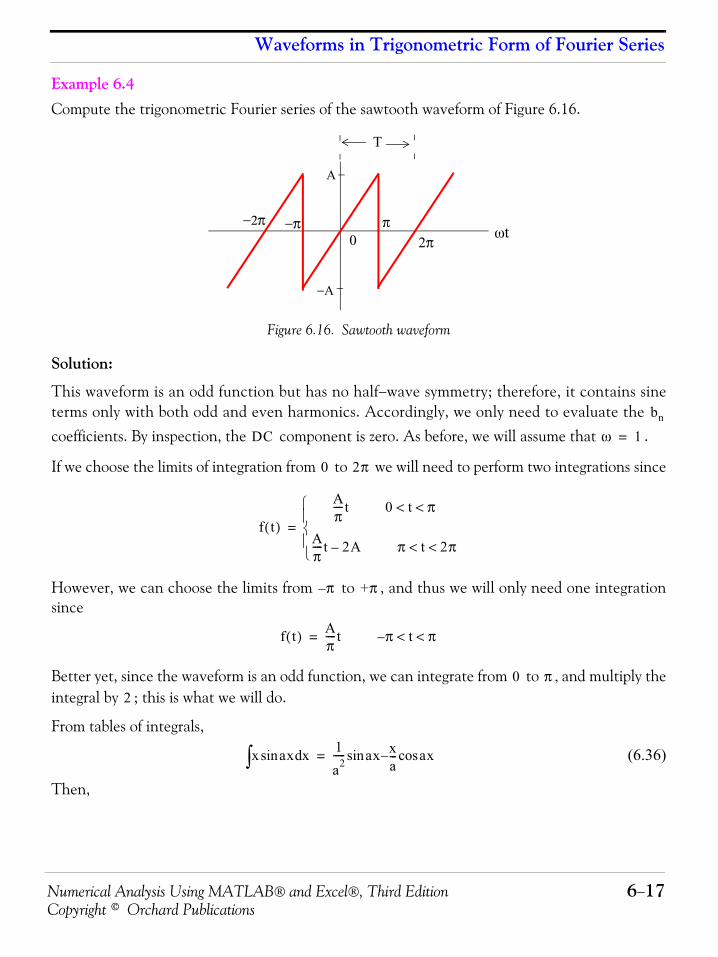
Numerical Analysis Using MATLAB® and Excel®, Third Edition 6−17Copyright © Orchard Publications
Waveforms in Trigonometric Form of Fourier Series
Example 6.4 Compute the trigonometric Fourier series of the sawtooth waveform of Figure 6.16.
Figure 6.16. Sawtooth waveform
Solution:
This waveform is an odd function but has no half−wave symmetry; therefore, it contains sineterms only with both odd and even harmonics. Accordingly, we only need to evaluate the coefficients. By inspection, the component is zero. As before, we will assume that .
If we choose the limits of integration from to we will need to perform two integrations since
However, we can choose the limits from to , and thus we will only need one integrationsince
Better yet, since the waveform is an odd function, we can integrate from to , and multiply theintegral by ; this is what we will do.
From tables of integrals,
(6.36)
Then,
0 2π
T
ωt
A
−A
π−π−2π
bn
DC ω 1=
0 2π
f t( )
Aπ----t 0 t π< <
Aπ----t 2A– π t 2π< <⎩
⎪⎨⎪⎧
=
π– +π
f t( ) Aπ----t= π– t π< <
0 π2
x ax xdsin∫1a2----- asin x x
a---– axcos=
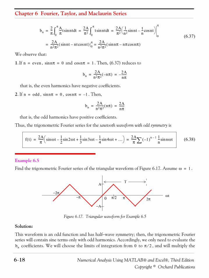
Chapter 6 Fourier, Taylor, and Maclaurin Series
6−18 Numerical Analysis Using MATLAB® and Excel®, Third EditionCopyright © Orchard Publications
(6.37)
We observe that:
1. If , and . Then, (6.37) reduces to
that is, the even harmonics have negative coefficients.
2. If , , . Then,
that is, the odd harmonics have positive coefficients.
Thus, the trigonometric Fourier series for the sawtooth waveform with odd symmetry is
(6.38)
Example 6.5
Find the trigonometric Fourier series of the triangular waveform of Figure 6.17. Assume .
Figure 6.17. Triangular waveform for Example 6.5
Solution:
This waveform is an odd function and has half−wave symmetry; then, the trigonometric Fourierseries will contain sine terms only with odd harmonics. Accordingly, we only need to evaluate the
coefficients. We will choose the limits of integration from to , and will multiply the
bn2π--- A
π----t ntsin td
0
π
∫2Aπ2------- t ntsin td
0
π
∫2Aπ2------- 1
n2----- ntsin t
n--- ntcos–⎝ ⎠
⎛ ⎞
0
π
= = =
2An2π2----------- ntsin nt ntcos–( ) 0
π 2An2π2----------- nπsin nπ nπcos–( )==
n even= nπsin 0= nπcos 1=
bn2A
n2π2----------- nπ–( ) 2A
nπ-------–= =
n odd= nπsin 0= nπcos 1–=
bn2A
n2π2----------- nπ( ) 2A
nπ-------= =
f t( ) 2Aπ
------- ωt 12--- 2ωt 1
3--- 3ωtsin 1
4--- 4ωt …+sin–+sin–sin⎝ ⎠
⎛ ⎞ 2Aπ
------- 1–( )n 1–∑1n--- nωtsin= =
ω 1=
0 2π
T
ωt
A
−A
π−π−2π
π/2
bn 0 π 2⁄
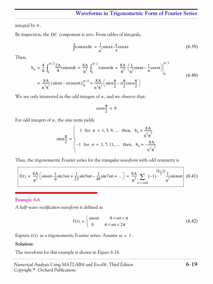
Numerical Analysis Using MATLAB® and Excel®, Third Edition 6−19Copyright © Orchard Publications
Waveforms in Trigonometric Form of Fourier Series
integral by .
By inspection, the component is zero. From tables of integrals,
(6.39)
Then,
(6.40)
We are only interested in the odd integers of , and we observe that:
For odd integers of , the sine term yields
Thus, the trigonometric Fourier series for the triangular waveform with odd symmetry is
(6.41)
Example 6.6 A half−wave rectification waveform is defined as
(6.42)
Express as a trigonometric Fourier series. Assume .
Solution:
The waveform for this example is shown in Figure 6.18.
4
DC
x ax xdsin∫1a2---- asin x x
a---– axcos=
bn4π--- 2A
π-------t ntsin td
0
π 2⁄
∫8Aπ2------- t ntsin td
0
π 2⁄
∫8Aπ2------- 1
n2----- ntsin t
n--- ntcos–⎝ ⎠
⎛ ⎞
0
π 2⁄= = =
8An2π2---------- ntsin nt ntcos–( ) 0
π 2⁄ 8An2π2---------- nπ
2---sin nπ
2--- nπ
2---cos–⎝ ⎠
⎛ ⎞==
n
nπ2---cos 0=
n
nπ2---sin
1 for n 1 5 9 … then bn8A
n2π2
-----------=, , , ,=
1– for n 3 7 11 … then bn8A
n2π2
-----------–=, , , ,=
⎩⎪⎪⎨⎪⎪⎧
=
f t( ) 8Aπ2------- ωsin t 1
9---– 3ωt 1
25------ 5ωtsin 1
49------ 7ωtsin …+–+sin⎝ ⎠
⎛ ⎞ 8Aπ2------- 1–( )
n 1–( )2
---------------- 1n2----- nsin ωt
n odd=∑= =
f t( )ωtsin 0 ωt π< <
0 π ωt 2π< <⎩⎨⎧
=
f t( ) ω 1=
Chapter 6 Fourier, Taylor, and Maclaurin Series
6−20 Numerical Analysis Using MATLAB® and Excel®, Third EditionCopyright © Orchard Publications
Figure 6.18. for Example 6.6
By inspection, the average is a non−zero value, and the waveform has neither odd nor even sym-metry. Therefore, we expect all terms to be present. The coefficients are found from
For this example,
and from tables of integrals
Then,
(6.43)
Using the trigonometric identities
and
we obtain
and
Then, by substitution into (6.43),
(6.44)
π– 3π0 π 2π2– π
f t( )
an
an1π--- f t( ) nt tdcos
0
2π
∫=
anAπ---- t nt tdcossin
0
π
∫Aπ---- 0 nt tdcos
π
2π
∫+=
mxsin( ) nxcos( ) xd∫ m n–( )xcos2 m n–( )
------------------------------– m n+( )xcos2 m n+( )
------------------------------- m2 n2≠( )–=
anAπ---- 1
2--- 1 n–( )tcos
1 n–--------------------------- 1 n+( )tcos
1 n+----------------------------+
0
π
–⎩ ⎭⎨ ⎬⎧ ⎫
=
A2π------– π nπ–( )cos
1 n–----------------------------- π nπ+( )cos
1 n+------------------------------+ 1
1 n–------------ 1
n 1+------------+–
⎩ ⎭⎨ ⎬⎧ ⎫
=
x y–( )cos x ycoscos xsinysin+=
x y+( )cos x y x ysinsin–coscos=
π nπ–( )cos π nπcoscos π nπsinsin+ nπcos–= =
π nπ+( )cos π nπcoscos π nπsinsin– nπcos–= =
anA2π------– nπcos–
1 n–------------------ nπcos–
1 n+------------------+ 2
1 n2–--------------–
⎩ ⎭⎨ ⎬⎧ ⎫ A
2π------ nπcos
1 n–--------------- nπcos
1 n+---------------+ 2
1 n2–--------------+
⎩ ⎭⎨ ⎬⎧ ⎫
= =
A2π------ nπ n nπ nπcos+cos+cos n nπcos–
1 n2–--------------------------------------------------------------------------------------- 2
1 n2–--------------+⎝ ⎠
⎛ ⎞ Aπ---- nπ 1+cos
1 n2–( )-------------------------⎝ ⎠⎛ ⎞ n 1≠==
Numerical Analysis Using MATLAB® and Excel®, Third Edition 6−21Copyright © Orchard Publications
Waveforms in Trigonometric Form of Fourier Series
Next, we can evaluate all the coefficients, except , from (6.44).
First, we will evaluate to obtain the value. By substitution of , we get Therefore, the value is
(6.45)
We cannot use (6.44) to obtain the value of ; therefore, we will evaluate the integral
From tables of integrals,
and thus,(6.46)
From (6.44) with , we get
(6.47)
(6.48)
We see that for odd integers of , . However, for , we get
(6.49)
(6.50)
(6.51)
and so on.
Now, we need to evaluate the coefficients. For this example,
an a1
a0 DC n 0= a0 2A π⁄=
DC12---a0
Aπ----=
a1
a1Aπ---- t t tdcossin
0
π
∫=
axsin( ) axcos( ) xd∫1
2a------ axsin( )2=
a1A2π------ tsin( )2
0
π0= =
n 2 3 4 5 …, , , ,=
a2Aπ---- 2π 1+cos
1 22–( )-------------------------⎝ ⎠⎛ ⎞ 2A
3π-------–= =
a3A 3π 1+cos( )
π 1 32–( )---------------------------------- 0= =
n an 0= n even=
a4A 4π 1+cos( )
π 1 42–( )---------------------------------- 2A
15π---------–= =
a6A 6π 1+cos( )
π 1 62–( )---------------------------------- 2A
35π---------–= =
a8A 8π 1+cos( )
π 1 82–( )---------------------------------- 2A
63π---------–= =
bn
bn A1π--- f t( ) nt tdsin
0
2π
∫Aπ---- t nt tdsinsin
0
π
∫Aπ---- 0 nt tdsin
π
2π
∫+= =
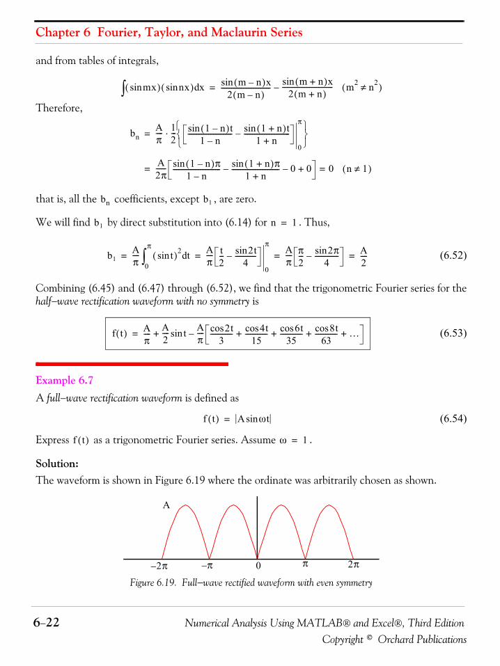
Chapter 6 Fourier, Taylor, and Maclaurin Series
6−22 Numerical Analysis Using MATLAB® and Excel®, Third EditionCopyright © Orchard Publications
and from tables of integrals,
Therefore,
that is, all the coefficients, except , are zero.
We will find by direct substitution into (6.14) for . Thus,
(6.52)
Combining (6.45) and (6.47) through (6.52), we find that the trigonometric Fourier series for thehalf−wave rectification waveform with no symmetry is
(6.53)
Example 6.7 A full−wave rectification waveform is defined as
(6.54)
Express as a trigonometric Fourier series. Assume .
Solution:The waveform is shown in Figure 6.19 where the ordinate was arbitrarily chosen as shown.
Figure 6.19. Full−wave rectified waveform with even symmetry
mxsin( ) nxsin( ) xd∫ m n–( )xsin2 m n–( )
----------------------------- m n+( )xsin2 m n+( )
------------------------------ m2 n2≠( )–=
bnAπ---- 1
2---⋅ 1 n–( )tsin
1 n–-------------------------- 1 n+( )tsin
1 n+---------------------------–
0
π
⎩ ⎭⎨ ⎬⎧ ⎫
=
A2π------ 1 n–( )πsin
1 n–---------------------------- 1 n+( )πsin
1 n+----------------------------– 0– 0+ 0 n 1≠( )==
bn b1
b1 n 1=
b1Aπ---- tsin( )2 td
0
π
∫Aπ---- t
2--- 2tsin
4------------–
0
πAπ---- π
2--- 2πsin
4--------------– A
2----= = = =
f t( ) Aπ---- A
2---- tsin A
π---- 2tcos
3------------- 4tcos
15------------- 6tcos
35------------- 8tcos
63------------- …+ + + +–+=
f t( ) A ωtsin=
f t( ) ω 1=
0 2 4 6 8 1 0 1 20
0 . 1
0 . 2
0 . 3
0 . 4
0 . 5
0 . 6
0 . 7
0 . 8
0 . 9
1
2π– 2πππ– 0
A
Numerical Analysis Using MATLAB® and Excel®, Third Edition 6−23Copyright © Orchard Publications
Waveforms in Trigonometric Form of Fourier Series
By inspection, the average is a non−zero value. We choose the period of the input sinusoid so thatthe output will be expressed in terms of the fundamental frequency. We also choose the limits ofintegration as and , we observe that the waveform has even symmetry.
Therefore, we expect only cosine terms to be present. The coefficients are found from
where for this example,
(6.55)
and from tables of integrals,
Since
we express (6.55) as
(6.56)
To simplify the last expression in (6.56), we make use of the trigonometric identities
and
Then, (6.56) simplifies to
(6.57)
Now, we can evaluate all the coefficients, except , from (6.57). First, we will evaluate to
π– +π
an
an1π--- f t( ) nt tdcos
0
2π
∫=
an1π--- A t nt tdcossin
π–
π
∫2Aπ
------- t nt tdcossin0
π
∫==
mxsin( ) nxcos( ) xd∫ m n–( )xcos2 n m–( )
------------------------------ m n+( )xcos2 m n+( )
------------------------------- m2 n2≠( )–=
x y–( )cos y x–( )cos x ycoscos xsinysin+= =
an2Aπ
------- 12---⋅ n 1–( )tcos
n 1–--------------------------- n 1+( )tcos
n 1+----------------------------–
0
π
⎩ ⎭⎨ ⎬⎧ ⎫
=
Aπ---- n 1–( )πcos
n 1–----------------------------- n 1+( )πcos
n 1+-----------------------------– 1
n 1–------------ 1
n 1+------------––
⎩ ⎭⎨ ⎬⎧ ⎫
=
Aπ---- 1 nπ π+( )cos–
n 1+--------------------------------------- nπ π–( ) 1–cos
n 1–--------------------------------------+=
nπ π+( )cos nπ πcoscos nπsinπsin– nπcos–= =
nπ π–( )cos nπ πcoscos nπsinπsin+ nπcos–= =
anAπ---- 1 nπcos+
n 1+------------------------- 1 nπcos+
n 1–-------------------------– A
π---- 2– n 1–( ) nπcos+ n 1+( ) nπcos–
n2 1–-------------------------------------------------------------------------------------= =
2A– nπ 1+cos( )π n2 1–( )
----------------------------------------- n 1≠=
an a1 a0
Chapter 6 Fourier, Taylor, and Maclaurin Series
6−24 Numerical Analysis Using MATLAB® and Excel®, Third EditionCopyright © Orchard Publications
obtain the value. By substitution of , we get
Therefore, the value is
(6.58)
From (6.57) we observe that for all , other than , .To obtain the value of , we must evaluate the integral
From tables of integrals,
and thus,
(6.59)
For , from (6.57) we get
(6.60)
(6.61)
(6.62)
(6.63)
and so on. Then, combining the terms of (6.58) and (6.60) through (6.63) we get
(6.64)
Therefore, the trigonometric form of the Fourier series for the full−wave rectification waveform witheven symmetry is
DC n 0=
a04Aπ
-------=
DC
12---a0
2Aπ
-------=
n odd= n 1= an 0=
a1
a11π--- t t tdcossin
0
π
∫=
axsin( ) axcos( ) xd∫1
2a------ axsin( )2=
a11
2π------ tsin( )2
0
π0= =
n even=
a22A– 2π 1+cos( )
π 22 1–( )----------------------------------------- 4A
3π-------–= =
a42A– 4π 1+cos( )
π 42 1–( )----------------------------------------- 4A
15π---------–= =
a62A– 6π 1+cos( )
π 62 1–( )----------------------------------------- 4A
35π---------–= =
a82A– 8π 1+cos( )
π 82 1–( )----------------------------------------- 4A
63π---------–= =
f t( ) 2Aπ
------- 4Aπ
------- 2ωtcos3
------------------ 4ωtcos15
------------------ 6ωtcos35
------------------ 8ωtcos63
------------------ …+ + + +⎩ ⎭⎨ ⎬⎧ ⎫
–=
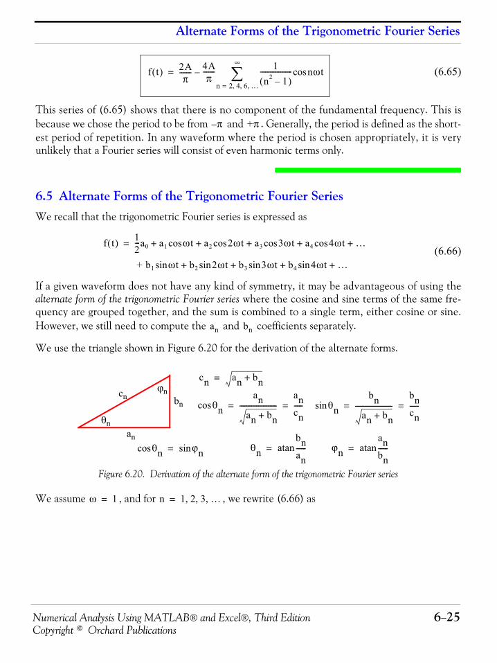
Numerical Analysis Using MATLAB® and Excel®, Third Edition 6−25Copyright © Orchard Publications
Alternate Forms of the Trigonometric Fourier Series
(6.65)
This series of (6.65) shows that there is no component of the fundamental frequency. This isbecause we chose the period to be from and . Generally, the period is defined as the short-est period of repetition. In any waveform where the period is chosen appropriately, it is veryunlikely that a Fourier series will consist of even harmonic terms only.
6.5 Alternate Forms of the Trigonometric Fourier SeriesWe recall that the trigonometric Fourier series is expressed as
(6.66)
If a given waveform does not have any kind of symmetry, it may be advantageous of using thealternate form of the trigonometric Fourier series where the cosine and sine terms of the same fre-quency are grouped together, and the sum is combined to a single term, either cosine or sine.However, we still need to compute the and coefficients separately.
We use the triangle shown in Figure 6.20 for the derivation of the alternate forms.
Figure 6.20. Derivation of the alternate form of the trigonometric Fourier series
We assume , and for , we rewrite (6.66) as
f t( ) 2Aπ
------- 4Aπ
------- 1n2 1–( )
------------------- nωtcosn 2 4 6 …, , ,=
∞
∑–=
π– +π
f t( ) 12---a0 a1 ωtcos a2 2ωtcos a3 3ωt a4 4ωtcos+cos …+ + + +=
+ b1 ωtsin b2 2ωtsin b3 3ωt b4 4ωtsin+sin …+ + +
an bn
an
bncn
θn
ϕn
θnsinbn
an bn+----------------------
bncn------= =
cn an bn+=
θncosan
an bn+----------------------
ancn-----= =
θnbnan------atan= ϕn
anbn------atan=θncos ϕnsin=
ω 1= n 1 2 3 …, , ,=
Chapter 6 Fourier, Taylor, and Maclaurin Series
6−26 Numerical Analysis Using MATLAB® and Excel®, Third EditionCopyright © Orchard Publications
and, in general, for , we get
(6.67)
Similarly,
and, in general, where , we get
(6.68)
The series of (6.67) and (6.68) can be expressed as phasors. Since it is customary to use the cosinefunction in the time domain to phasor transformation, we choose to use the transformation of(6.63) below.
(6.69)
Example 6.8 Find the first 5 terms of the alternate form of the trigonometric Fourier series for the waveform ofFigure 6.21.
f t( ) 12---a0 c1
a1
c1---- t
b1
c1----- tsin+cos⎝ ⎠
⎛ ⎞ c2a2
c2---- 2t
b2
c2----- 2tsin+cos⎝ ⎠
⎛ ⎞ …+ + +=
+ cnancn----- nt
bncn----- ntsin+cos⎝ ⎠
⎛ ⎞
12---a0 c1
θ1 t θ1 tsinsin+coscos
t θ1–( )cos⎝ ⎠⎛ ⎞ c2
θ2 2t θ2 2tsinsin+coscos
2t θ2–( )cos⎝ ⎠⎛ ⎞ …+ + +=
+ cn
θn nt θn ntsinsin+coscos
nt θn–( )cos⎝ ⎠⎛ ⎞
⎧ ⎪ ⎪ ⎪ ⎪ ⎨ ⎪ ⎪ ⎪ ⎪ ⎩ ⎧ ⎪ ⎪ ⎪ ⎪ ⎨ ⎪ ⎪ ⎪ ⎪ ⎩
⎧ ⎪ ⎪ ⎪ ⎪ ⎨ ⎪ ⎪ ⎪ ⎪ ⎩
ω 1≠
f t( ) 12---a0 cn nωt θn–( )cos
n 1=
∞
∑+ 12---a0 cn nωt
bnan-----atan–⎝ ⎠
⎛ ⎞cosn 1=
∞
∑+= =
f t( ) 12---a0 c1
ϕ1sin t ϕ1cos tsin+cos
t ϕ1+( )sin⎝ ⎠⎛ ⎞+=
c2
ϕ2sin 2t ϕ2cos 2tsin+cos
2t ϕ2+( )sin⎝ ⎠⎛ ⎞ … cn
ϕnsin nt ϕncos ntsin+cos
nt ϕn+( )sin⎝ ⎠⎛ ⎞++
⎧ ⎪ ⎪ ⎪ ⎪ ⎨ ⎪ ⎪ ⎪ ⎪ ⎩
⎧ ⎪ ⎪ ⎪ ⎪ ⎨ ⎪ ⎪ ⎪ ⎪ ⎩ ⎧ ⎪ ⎪ ⎪ ⎪ ⎨ ⎪ ⎪ ⎪ ⎪ ⎩
ω 1≠
f t( ) 12---a0 cn nωt ϕn+( )sin
n 1=
∞
∑+12---a0 cn nωt
anbn-----atan+⎝ ⎠
⎛ ⎞sinn 1=
∞
∑+= =
12---a0 cn nωt
bnan-----atan–⎝ ⎠
⎛ ⎞cosn 1=
∞
∑+ 12---a0 cn
bnan-----atan–∠
n 1=
∞
∑+⇔
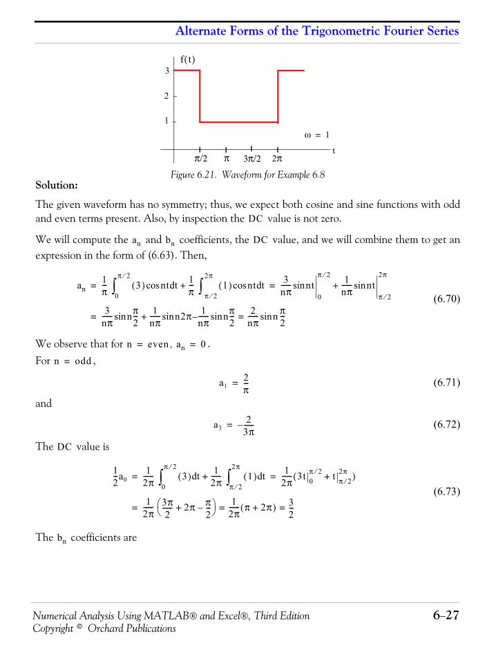
Numerical Analysis Using MATLAB® and Excel®, Third Edition 6−27Copyright © Orchard Publications
Alternate Forms of the Trigonometric Fourier Series
Figure 6.21. Waveform for Example 6.8Solution:
The given waveform has no symmetry; thus, we expect both cosine and sine functions with oddand even terms present. Also, by inspection the value is not zero.
We will compute the and coefficients, the value, and we will combine them to get anexpression in the form of (6.63). Then,
(6.70)
We observe that for , .For ,
(6.71)
and
(6.72)
The value is
(6.73)
The coefficients are
1
2
3
2πππ/2 3π/2t
f t( )
ω 1=
DC
an bn DC
an1π--- 3( ) ntcos t 1
π--- 1( ) ntcos td
π 2⁄
2π
∫+d0
π 2⁄
∫3
nπ------ ntsin
0
π 2⁄ 1nπ------ ntsin
π 2⁄
2π+= =
3nπ------ nπ
2---sin 1
nπ------ n2πsin 1
nπ------ nπ
2---sin–+
2nπ------ n π
2---sin==
n even= an 0=
n odd=
a12π---=
a32
3π------–=
DC
12---a0
12π------ 3( ) td
0
π 2⁄
∫1
2π------ 1( ) td
π 2⁄
2π
∫+1
2π------ 3t 0
π 2⁄ t π 2⁄2π+( )= =
12π------ 3π
2------ 2π π
2---–+⎝ ⎠
⎛ ⎞ 12π------ π 2π+( ) 3
2---= ==
bn
Chapter 6 Fourier, Taylor, and Maclaurin Series
6−28 Numerical Analysis Using MATLAB® and Excel®, Third EditionCopyright © Orchard Publications
(6.74)
Then,(6.75)
(6.76)
(6.77)
(6.78)From (6.69),
where
(6.79)
Thus, for , we get:
(6.80)
Similarly,
(6.81)
(6.82)
and
(6.83)
Combining the terms of (6.73) and (6.80) through (6.83), we find that the alternate form of thetrigonometric Fourier series representing the waveform of this example is
bn1π--- 3( ) ntsin t 1
π--- 1( ) ntsin td
π 2⁄
2π
∫+d0
π 2⁄
∫3–
nπ------ ntcos
0
π 2⁄ 1–nπ------ ntcos
π 2⁄
2π+= =
3–nπ------ nπ
2---cos 3
nπ------ 1–
nπ------ n2πcos 1
nπ------ nπ
2---cos+ + + 1
nπ------ 3 n2πcos–( ) 2
nπ------= ==
b1 2 π⁄=
b2 1 π⁄=
b3 2 3π⁄=
b4 1 2π⁄=
12---a0 cn nωt
bnan-----atan–⎝ ⎠
⎛ ⎞cosn 1=
∞
∑+ 12---a0 cn
bnan-----atan–∠
n 1=
∞
∑+⇔
cnbnan-----atan–∠ an
2 bn2+
bnan-----atan–∠ an
2 bn2+ θn–∠ an jbn–= = =
n 1 2 3 and 4, , ,=
a1 jb1– 2π--- j2
π---–
2π---⎝ ⎠⎛ ⎞ 2 2
π---⎝ ⎠⎛ ⎞ 2
+ 45°–∠= =
8
π2------ 45°–∠ 2 2
π---------- 45°–∠ 2 2
π---------- ωt 45°–( )cos⇔==
a2 jb2– 0 j1π---–
1π--- 90°–∠= =
1π--- 2ωt 90°–( )cos⇔
a3 jb3– 23π------– j 2
3π------–
2 23π
---------- 135°–∠= =2 23π
---------- 3ωt 135°–( )cos⇔
a4 jb4– 0 j 12π------– 1
2π------ 90°–∠= = 1
2π------ 4ωt 90°–( )cos⇔
Numerical Analysis Using MATLAB® and Excel®, Third Edition 6−29Copyright © Orchard Publications
The Exponential Form of the Fourier Series
(6.84)
6.6 The Exponential Form of the Fourier Series The Fourier series are often expressed in exponential form. The advantage of the exponentialform is that we only need to perform one integration rather than two, one for the , andanother for the coefficients in the trigonometric form of the series. Moreover, in most casesthe integration is simpler.
The exponential form is derived from the trigonometric form by substitution of
(6.85)
and
(6.86)
into . Thus,
(6.87)
and grouping terms with same exponents, we get
(6.88)
The terms of (6.88) in parentheses are usually denoted as
(6.89)
(6.90)
(6.91)
f t( ) 32--- 1
π--- [2 2 ωt 45°–( )cos 2ωt 90°–( )cos++=
+ 2 23
---------- 3ωt 135°–( )cos 12--- 4ωt 90°–( )cos … ]+ +
an
bn
ωtcos e jωt e jωt–+2
----------------------------=
ωtsin e jωt e jωt––j2
---------------------------=
f t( )
f t( ) 12---a0 a1
e jωt e jωt–+2
----------------------------⎝ ⎠⎛ ⎞ a2
e j2ωt e j2ωt–+2
---------------------------------⎝ ⎠⎛ ⎞
… b1e jωt e jωt––
j2---------------------------⎝ ⎠⎛ ⎞ b2
e j2ωt e j2ωt––j2
--------------------------------⎝ ⎠⎛ ⎞ …
+ + +
+ + +
=
f t( ) … a2
2---- b2
j2-----–⎝ ⎠
⎛ ⎞ e j2ωt– a1
2---- b1
j2-----–⎝ ⎠
⎛ ⎞ e jωt– 12---a0
a1
2---- b1
j2-----+⎝ ⎠
⎛ ⎞ ejωt a2
2---- b2
j2-----+⎝ ⎠
⎛ ⎞ ej2ωt+ + + + +=
C n–12--- an
bnj
-----–⎝ ⎠⎛ ⎞ 1
2--- an jbn+( )= =
Cn12--- an
bnj
-----+⎝ ⎠⎛ ⎞ 1
2--- an j– bn( )= =
C012---a0=
Chapter 6 Fourier, Taylor, and Maclaurin Series
6−30 Numerical Analysis Using MATLAB® and Excel®, Third EditionCopyright © Orchard Publications
Then, (6.88) is written as
(6.92)
We must remember that the coefficients, except , are complex and occur in complex conju-gate pairs, that is,
(6.93)
We can derive a general expression for the complex coefficients , by multiplying both sides of
(6.92) by and integrating over one period, as we did in the derivation of the and coefficients of the trigonometric form. Then, with ,
(6.94)
We observe that all the integrals on the right side of (6.97) are zero except the last. Therefore,
or
and, in general, for ,
(6.95)
or
(6.96)
We can derive the trigonometric Fourier series from the exponential series by addition and sub-traction of the exponential form coefficients and . Thus, from (6.89) and (6.90),
f t( ) … C 2– e j2ωt– C 1– e jωt– C0 C1e jωt C2ej2ωt …+ + + + + +=
Ci C0
C n– Cn∗=
Cn
e jnωt– an bn
ω 1=
f t( )e jnt– td0
2π
∫ … C 2– e j2t– e jnt– td0
2π
∫ C 1– e jt– e jnt– td0
2π
∫ + C0 e jnt– td
0
2π
∫ C1 e jte jnt– td0
2π
∫ + C2 e j2te jnt– td
0
2π
∫ … Cne jnte jnt– td0
2π
∫
+ +
+
+ +
=
f t( )e jnt– td0
2π
∫ Cne jnte jnt– td0
2π
∫ Cn td0
2π
∫ 2πCn= = =
Cn1
2π------ f t( )e jnt– td
0
2π
∫=
ω 1≠
Cn1
2π------ f t( )e jnωt– ωt( )d
0
2π
∫=
Cn1T--- f t( )e jnωt– ωt( )d
0
T
∫=
Cn C n–
Cn C n–+12--- an jbn– an jbn+ +( )=
Numerical Analysis Using MATLAB® and Excel®, Third Edition 6−31Copyright © Orchard Publications
The Exponential Form of the Fourier Series
or
(6.97)
Similarly,
(6.98)
or
(6.99)
Symmetry in Exponential Series
1. For even functions, all coefficients are real
We recall from (6.89) and (6.90) that
(6.100)
and
(6.101)
Since even functions have no sine terms, the coefficients in (6.100) and (6.101) are zero.Therefore, both and are real.
2. For odd functions, all coefficients are imaginary
Since odd functions have no cosine terms, the coefficients in (6.100) and (6.101) are zero.Therefore, both and are imaginary.
3. If there is half−wave symmetry, for
We recall from the trigonometric Fourier series that if there is half−wave symmetry, all evenharmonics are zero. Therefore, in (6.100) and (6.101) the coefficients and are both zerofor , and thus, both and are also zero for .
4. If there is no symmetry, is complex.
5. always
This can be seen in (6.100) and (6.101)
an Cn C n–+=
Cn C n–– 12--- an jbn– an– j– bn( )=
bn j Cn C n––( )=
Ci
C n–12--- an
bnj
-----–⎝ ⎠⎛ ⎞ 1
2--- an jbn+( )= =
Cn12--- an
bnj
-----+⎝ ⎠⎛ ⎞ 1
2--- an j– bn( )= =
bn
C n– Cn
Ci
an
C n– Cn
Cn 0= n even=
an bn
n even= C n– Cn n even=
f t( )
C n– Cn∗=
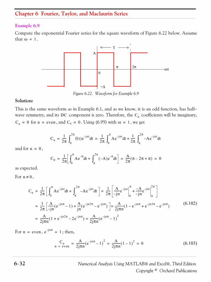
Chapter 6 Fourier, Taylor, and Maclaurin Series
6−32 Numerical Analysis Using MATLAB® and Excel®, Third EditionCopyright © Orchard Publications
Example 6.9 Compute the exponential Fourier series for the square waveform of Figure 6.22 below. Assumethat .
Figure 6.22. Waveform for Example 6.9
Solution:
This is the same waveform as in Example 6.1, and as we know, it is an odd function, has half−wave symmetry, and its component is zero. Therefore, the coefficients will be imaginary,
for , and . Using (6.95) with , we get
and for ,
as expected.
For ,
(6.102)
For , ; then,
(6.103)
ω 1=
0π 2π
TA
−A
ωt
DC Cn
Cn 0= n even= C0 0= ω 1=
Cn1
2π------ f t( )e jnt– td
0
2π
∫1
2π------ Ae jnt– td
0
π
∫1
2π------ A– e jnt– td
π
2π
∫+= =
n 0=
C01
2π------ Ae 0– td
0
π
∫ A–( )e 0– tdπ
2π
∫+A2π------ π 2π– π+( ) 0= = =
n 0≠
Cn1
2π------ Ae jnt– td
0
π
∫ A– e jnt– tdπ
2π
∫+ 12π------ A
jn–--------e jnt–
0
π A–jn–
--------e jnt–
π
2π+= =
12π------ A
jn–-------- e jnπ– 1–( ) A
jn----- e jn2π– e jnπ––( )+
A2jπn------------ 1 e jnπ–– e jn2π– e jnπ––+( )==
A2jπn------------ 1 e jn2π– 2e jnπ––+( ) A
2jπn------------ e jnπ– 1–( )
2==
n even= e jnπ– 1=
Cnn even=
A2jπn------------ e jnπ– 1–( )
2 A2jπn------------ 1 1–( )2 0= = =
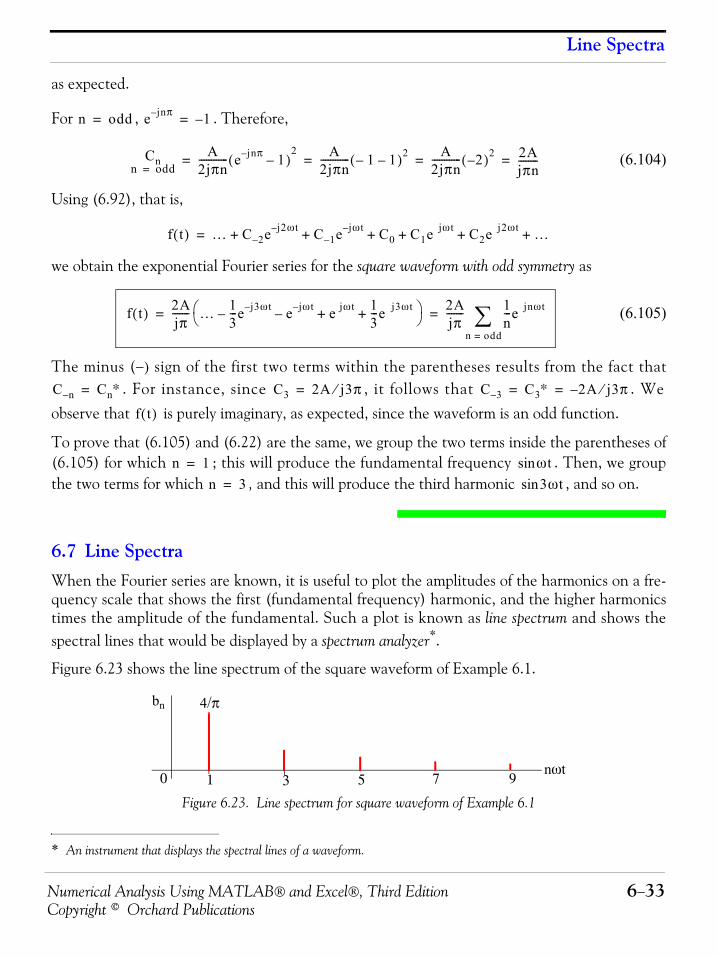
Numerical Analysis Using MATLAB® and Excel®, Third Edition 6−33Copyright © Orchard Publications
Line Spectra
as expected.
For , . Therefore,
(6.104)
Using (6.92), that is,
we obtain the exponential Fourier series for the square waveform with odd symmetry as
(6.105)
The minus (−) sign of the first two terms within the parentheses results from the fact that. For instance, since , it follows that . We
observe that is purely imaginary, as expected, since the waveform is an odd function.
To prove that (6.105) and (6.22) are the same, we group the two terms inside the parentheses of(6.105) for which ; this will produce the fundamental frequency . Then, we groupthe two terms for which , and this will produce the third harmonic , and so on.
6.7 Line SpectraWhen the Fourier series are known, it is useful to plot the amplitudes of the harmonics on a fre-quency scale that shows the first (fundamental frequency) harmonic, and the higher harmonicstimes the amplitude of the fundamental. Such a plot is known as line spectrum and shows thespectral lines that would be displayed by a spectrum analyzer*.
Figure 6.23 shows the line spectrum of the square waveform of Example 6.1.
Figure 6.23. Line spectrum for square waveform of Example 6.1
* An instrument that displays the spectral lines of a waveform.
n odd= e jnπ– 1–=
Cnn odd=
A2jπn------------ e jnπ– 1–( )
2 A2jπn------------ 1– 1–( )2 A
2jπn------------ 2–( )2 2A
jπn--------= = = =
f t( ) … C 2– e j2ωt– C 1– e jωt– C0 C1e jωt C2e j2ωt …+ + + + + +=
f t( ) 2Ajπ------- … 1
3---e j3ωt–– e jωt–– e jωt 1
3---e j3ωt+ +⎝ ⎠
⎛ ⎞ 2Ajπ------- 1
n---e jnωt
n odd=∑= =
C n– Cn∗= C3 2A j3π⁄= C 3– C3∗ 2A– j3π⁄= =
f t( )
n 1= ωtsinn 3= 3ωtsin
bn
nωt0 1 3 5 7 9
4/π
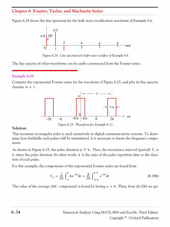
Chapter 6 Fourier, Taylor, and Maclaurin Series
6−34 Numerical Analysis Using MATLAB® and Excel®, Third EditionCopyright © Orchard Publications
Figure 6.24 shows the line spectrum for the half−wave rectification waveform of Example 6.6.
Figure 6.24. Line spectrum for half−wave rectifier of Example 6.6
The line spectra of other waveforms can be easily constructed from the Fourier series.
Example 6.10 Compute the exponential Fourier series for the waveform of Figure 6.25, and plot its line spectra.Assume .
Figure 6.25. Waveform for Example 6.11Solution:This recurrent rectangular pulse is used extensively in digital communications systems. To deter-mine how faithfully such pulses will be transmitted, it is necessary to know the frequency compo-nents.
As shown in Figure 6.25, the pulse duration is . Thus, the recurrence interval (period) , is times the pulse duration. In other words, is the ratio of the pulse repetition time to the dura-
tion of each pulse.
For this example, the components of the exponential Fourier series are found from
(6.106)
The value of the average ( component) is found by letting . Then, from (6.106) we get
nωt0 1
2 4 6 8
A/πA/2
DC
ω 1=
0−π/κ 2π
T
ωt
A
ππ/κ
T/κ
−π−2π
T k⁄ Tk k
Cn1
2π------ Ae jnt– td
π–
π
∫A2π------ e jnt– td
π k⁄–
π k⁄
∫= =
DC n 0=
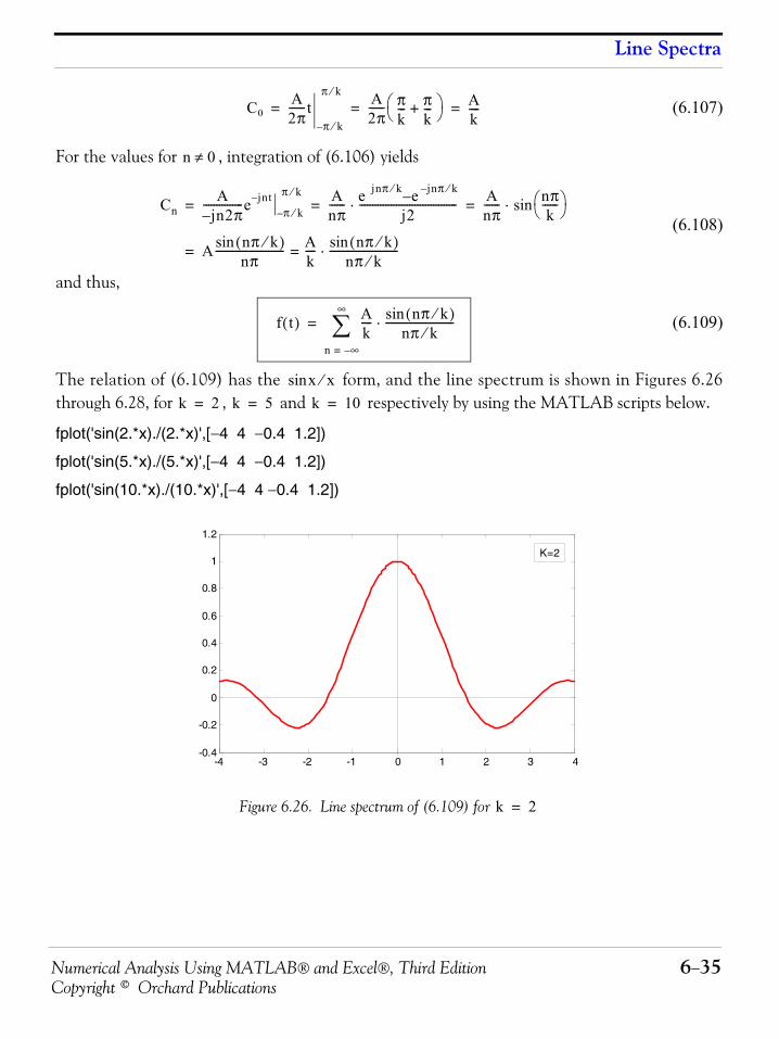
Numerical Analysis Using MATLAB® and Excel®, Third Edition 6−35Copyright © Orchard Publications
Line Spectra
(6.107)
For the values for , integration of (6.106) yields
(6.108)
and thus,
(6.109)
The relation of (6.109) has the form, and the line spectrum is shown in Figures 6.26through 6.28, for , and respectively by using the MATLAB scripts below.
fplot('sin(2.*x)./(2.*x)',[−4 4 −0.4 1.2])
fplot('sin(5.*x)./(5.*x)',[−4 4 −0.4 1.2])
fplot('sin(10.*x)./(10.*x)',[−4 4 −0.4 1.2])
Figure 6.26. Line spectrum of (6.109) for
C0A2π------t
π k⁄–
π k⁄ A2π------ π
k--- π
k---+⎝ ⎠
⎛ ⎞ Ak----= = =
n 0≠
CnA
jn2– π---------------e jnt–
π k⁄–
π k⁄ Anπ------ e jnπ k⁄ e jnπ k⁄––
j2-------------------------------------⋅ A
nπ------ nπ
k------⎝ ⎠⎛ ⎞sin⋅= = =
A nπ k⁄( )sinnπ
-------------------------- Ak---- nπ k⁄( )sin
nπ k⁄--------------------------⋅==
f t( ) Ak---- nπ k⁄( )sin
nπ k⁄--------------------------⋅
n ∞–=
∞
∑=
xsin x⁄k 2= k 5= k 10=
-4 -3 -2 -1 0 1 2 3 4-0.4
-0.2
0
0.2
0.4
0.6
0.8
1
1.2
K=2
k 2=
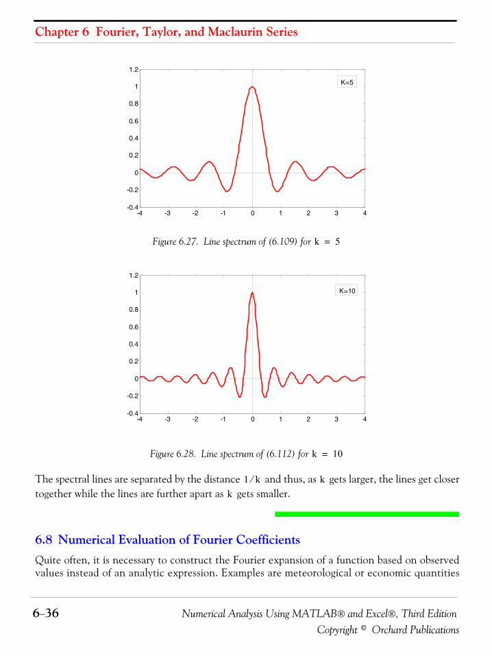
Chapter 6 Fourier, Taylor, and Maclaurin Series
6−36 Numerical Analysis Using MATLAB® and Excel®, Third EditionCopyright © Orchard Publications
Figure 6.27. Line spectrum of (6.109) for
Figure 6.28. Line spectrum of (6.112) for
The spectral lines are separated by the distance and thus, as gets larger, the lines get closertogether while the lines are further apart as gets smaller.
6.8 Numerical Evaluation of Fourier CoefficientsQuite often, it is necessary to construct the Fourier expansion of a function based on observedvalues instead of an analytic expression. Examples are meteorological or economic quantities
-4 -3 -2 -1 0 1 2 3 4-0.4
-0.2
0
0.2
0.4
0.6
0.8
1
1.2
K=5
k 5=
-4 -3 -2 -1 0 1 2 3 4-0.4
-0.2
0
0.2
0.4
0.6
0.8
1
1.2
K=10
k 10=
1 k⁄ kk
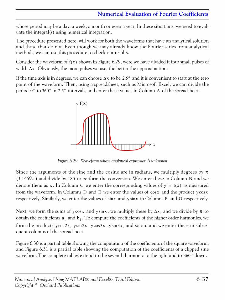
Numerical Analysis Using MATLAB® and Excel®, Third Edition 6−37Copyright © Orchard Publications
Numerical Evaluation of Fourier Coefficients
whose period may be a day, a week, a month or even a year. In these situations, we need to eval-uate the integral(s) using numerical integration.
The procedure presented here, will work for both the waveforms that have an analytical solutionand those that do not. Even though we may already know the Fourier series from analyticalmethods, we can use this procedure to check our results.
Consider the waveform of shown in Figure 6.29, were we have divided it into small pulses ofwidth . Obviously, the more pulses we use, the better the approximation.
If the time axis is in degrees, we can choose to be and it is convenient to start at the zeropoint of the waveform. Then, using a spreadsheet, such as Microsoft Excel, we can divide theperiod to in intervals, and enter these values in Column of the spreadsheet.
Figure 6.29. Waveform whose analytical expression is unknown
Since the arguments of the sine and the cosine are in radians, we multiply degrees by (3.1459...) and divide by to perform the conversion. We enter these in Column and wedenote them as . In Column we enter the corresponding values of as measuredfrom the waveform. In Columns and we enter the values of and the product respectively. Similarly, we enter the values of and in Columns and respectively.
Next, we form the sums of and , we multiply these by , and we divide by toobtain the coefficients and . To compute the coefficients of the higher order harmonics, weform the products , , , , and so on, and we enter these in subse-quent columns of the spreadsheet.
Figure 6.30 is a partial table showing the computation of the coefficients of the square waveform,and Figure 6.31 is a partial table showing the computation of the coefficients of a clipped sinewaveform. The complete tables extend to the seventh harmonic to the right and to down.
f x( )Δx
Δx 2.5°
0° 360° 2.5° A
x
f x( )
π180 B
x C y f x( )=
D E xcos y xcosxsin y xsin F G
y xcos y xsin Δx πa1 b1
y 2xcos y 2xsin y 3xcos y 3xsin
360°
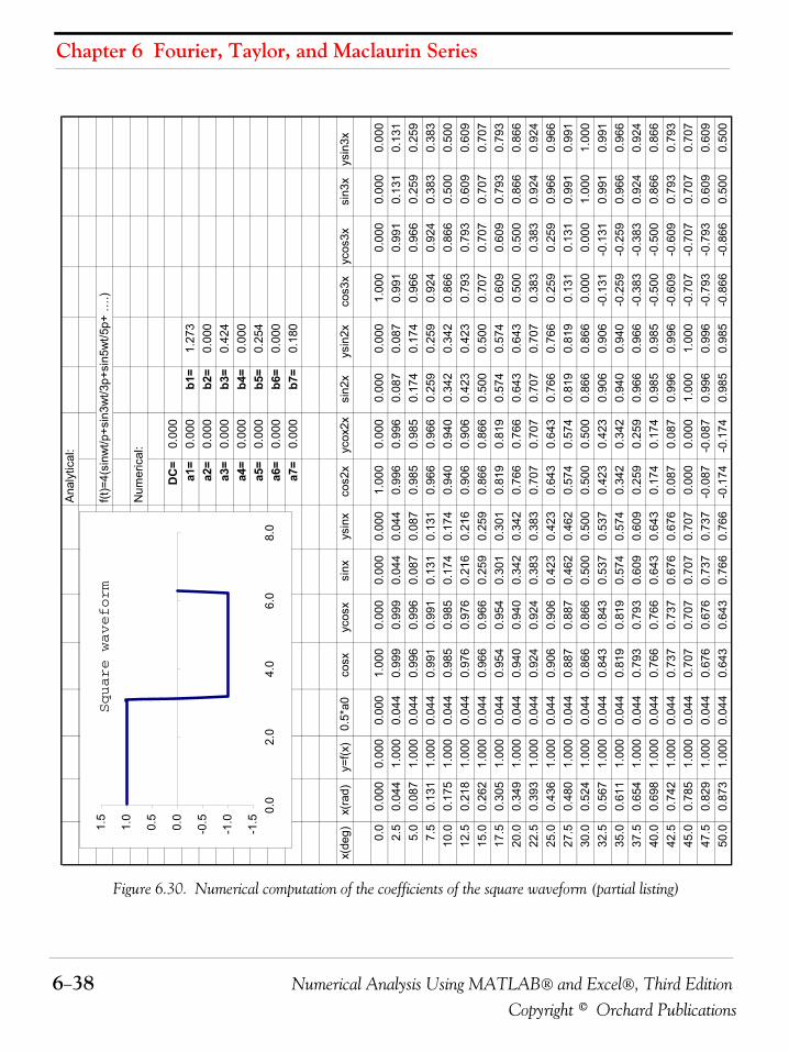
Chapter 6 Fourier, Taylor, and Maclaurin Series
6−38 Numerical Analysis Using MATLAB® and Excel®, Third EditionCopyright © Orchard Publications
Figure 6.30. Numerical computation of the coefficients of the square waveform (partial listing)
Ana
lytic
al:
f(t)=
4(si
nwt/p
+sin
3wt/3
p+si
n5w
t/5p+
….)
Num
eric
al:
Ave
rage
=D
C=
0.00
0a1
=0.
000
b1=
1.27
3a2
=0.
000
b2=
0.00
0a3
=0.
000
b3=
0.42
4a4
=0.
000
b4=
0.00
0a5
=0.
000
b5=
0.25
4a6
=0.
000
b6=
0.00
0
a7
=0.
000
b7=
0.18
0
x(de
g)x(
rad)
y=f(x
)0.
5*a0
co
sxyc
osx
sinx
ysin
xco
s2x
ycox
2xsi
n2x
ysin
2xco
s3x
ycos
3xsi
n3x
ysin
3x
0.0
0.00
00.
000
0.00
01.
000
0.00
00.
000
0.00
01.
000
0.00
00.
000
0.00
01.
000
0.00
00.
000
0.00
02.
50.
044
1.00
00.
044
0.99
90.
999
0.04
40.
044
0.99
60.
996
0.08
70.
087
0.99
10.
991
0.13
10.
131
5.0
0.08
71.
000
0.04
40.
996
0.99
60.
087
0.08
70.
985
0.98
50.
174
0.17
40.
966
0.96
60.
259
0.25
97.
50.
131
1.00
00.
044
0.99
10.
991
0.13
10.
131
0.96
60.
966
0.25
90.
259
0.92
40.
924
0.38
30.
383
10.0
0.17
51.
000
0.04
40.
985
0.98
50.
174
0.17
40.
940
0.94
00.
342
0.34
20.
866
0.86
60.
500
0.50
012
.50.
218
1.00
00.
044
0.97
60.
976
0.21
60.
216
0.90
60.
906
0.42
30.
423
0.79
30.
793
0.60
90.
609
15.0
0.26
21.
000
0.04
40.
966
0.96
60.
259
0.25
90.
866
0.86
60.
500
0.50
00.
707
0.70
70.
707
0.70
717
.50.
305
1.00
00.
044
0.95
40.
954
0.30
10.
301
0.81
90.
819
0.57
40.
574
0.60
90.
609
0.79
30.
793
20.0
0.34
91.
000
0.04
40.
940
0.94
00.
342
0.34
20.
766
0.76
60.
643
0.64
30.
500
0.50
00.
866
0.86
622
.50.
393
1.00
00.
044
0.92
40.
924
0.38
30.
383
0.70
70.
707
0.70
70.
707
0.38
30.
383
0.92
40.
924
25.0
0.43
61.
000
0.04
40.
906
0.90
60.
423
0.42
30.
643
0.64
30.
766
0.76
60.
259
0.25
90.
966
0.96
627
.50.
480
1.00
00.
044
0.88
70.
887
0.46
20.
462
0.57
40.
574
0.81
90.
819
0.13
10.
131
0.99
10.
991
30.0
0.52
41.
000
0.04
40.
866
0.86
60.
500
0.50
00.
500
0.50
00.
866
0.86
60.
000
0.00
01.
000
1.00
032
.50.
567
1.00
00.
044
0.84
30.
843
0.53
70.
537
0.42
30.
423
0.90
60.
906
-0.1
31-0
.131
0.99
10.
991
35.0
0.61
11.
000
0.04
40.
819
0.81
90.
574
0.57
40.
342
0.34
20.
940
0.94
0-0
.259
-0.2
590.
966
0.96
637
.50.
654
1.00
00.
044
0.79
30.
793
0.60
90.
609
0.25
90.
259
0.96
60.
966
-0.3
83-0
.383
0.92
40.
924
40.0
0.69
81.
000
0.04
40.
766
0.76
60.
643
0.64
30.
174
0.17
40.
985
0.98
5-0
.500
-0.5
000.
866
0.86
642
.50.
742
1.00
00.
044
0.73
70.
737
0.67
60.
676
0.08
70.
087
0.99
60.
996
-0.6
09-0
.609
0.79
30.
793
45.0
0.78
51.
000
0.04
40.
707
0.70
70.
707
0.70
70.
000
0.00
01.
000
1.00
0-0
.707
-0.7
070.
707
0.70
747
.50.
829
1.00
00.
044
0.67
60.
676
0.73
70.
737
-0.0
87-0
.087
0.99
60.
996
-0.7
93-0
.793
0.60
90.
609
50.0
0.87
31.
000
0.04
40.
643
0.64
30.
766
0.76
6-0
.174
-0.1
740.
985
0.98
5-0
.866
-0.8
660.
500
0.50
0
-1.5
-1.0
-0.50.0
0.5
1.0
1.5 0.
02.
04.
06.
08.
0
Square waveform
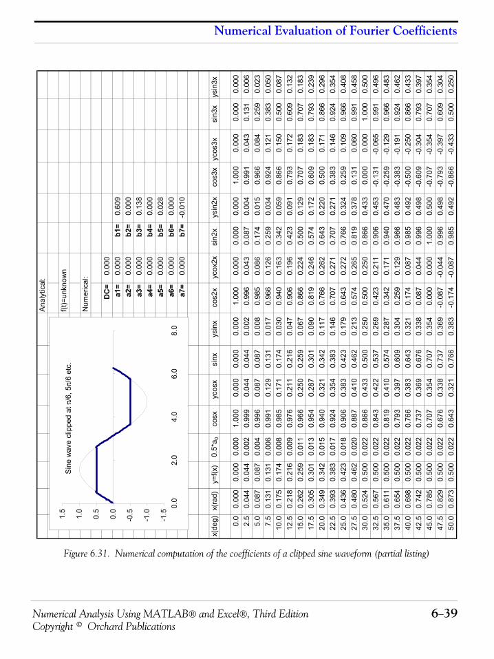
Numerical Analysis Using MATLAB® and Excel®, Third Edition 6−39Copyright © Orchard Publications
Numerical Evaluation of Fourier Coefficients
Figure 6.31. Numerical computation of the coefficients of a clipped sine waveform (partial listing)
Ana
lytic
al:
f(t)=
unkn
own
Num
eric
al:
DC
=0.
000
a1=
0.00
0b1
=0.
609
a2=
0.00
0b2
=0.
000
a3=
0.00
0b3
=0.
138
a4=
0.00
0b4
=0.
000
a5=
0.00
0b5
=0.
028
a6=
0.00
0b6
=0.
000
a7=
0.00
0b7
=-0
.010
x(de
g)x(
rad)
y=f(x
)0.
5*a 0
co
sxyc
osx
sinx
ysin
xco
s2x
ycox
2xsi
n2x
ysin
2xco
s3x
ycos
3xsi
n3x
ysin
3x
0.0
0.00
00.
000
0.00
01.
000
0.00
00.
000
0.00
01.
000
0.00
00.
000
0.00
01.
000
0.00
00.
000
0.00
02.
50.
044
0.04
40.
002
0.99
90.
044
0.04
40.
002
0.99
60.
043
0.08
70.
004
0.99
10.
043
0.13
10.
006
5.0
0.08
70.
087
0.00
40.
996
0.08
70.
087
0.00
80.
985
0.08
60.
174
0.01
50.
966
0.08
40.
259
0.02
37.
50.
131
0.13
10.
006
0.99
10.
129
0.13
10.
017
0.96
60.
126
0.25
90.
034
0.92
40.
121
0.38
30.
050
10.0
0.17
50.
174
0.00
80.
985
0.17
10.
174
0.03
00.
940
0.16
30.
342
0.05
90.
866
0.15
00.
500
0.08
712
.50.
218
0.21
60.
009
0.97
60.
211
0.21
60.
047
0.90
60.
196
0.42
30.
091
0.79
30.
172
0.60
90.
132
15.0
0.26
20.
259
0.01
10.
966
0.25
00.
259
0.06
70.
866
0.22
40.
500
0.12
90.
707
0.18
30.
707
0.18
317
.50.
305
0.30
10.
013
0.95
40.
287
0.30
10.
090
0.81
90.
246
0.57
40.
172
0.60
90.
183
0.79
30.
239
20.0
0.34
90.
342
0.01
50.
940
0.32
10.
342
0.11
70.
766
0.26
20.
643
0.22
00.
500
0.17
10.
866
0.29
622
.50.
393
0.38
30.
017
0.92
40.
354
0.38
30.
146
0.70
70.
271
0.70
70.
271
0.38
30.
146
0.92
40.
354
25.0
0.43
60.
423
0.01
80.
906
0.38
30.
423
0.17
90.
643
0.27
20.
766
0.32
40.
259
0.10
90.
966
0.40
827
.50.
480
0.46
20.
020
0.88
70.
410
0.46
20.
213
0.57
40.
265
0.81
90.
378
0.13
10.
060
0.99
10.
458
30.0
0.52
40.
500
0.02
20.
866
0.43
30.
500
0.25
00.
500
0.25
00.
866
0.43
30.
000
0.00
01.
000
0.50
032
.50.
567
0.50
00.
022
0.84
30.
422
0.53
70.
269
0.42
30.
211
0.90
60.
453
-0.1
31-0
.065
0.99
10.
496
35.0
0.61
10.
500
0.02
20.
819
0.41
00.
574
0.28
70.
342
0.17
10.
940
0.47
0-0
.259
-0.1
290.
966
0.48
337
.50.
654
0.50
00.
022
0.79
30.
397
0.60
90.
304
0.25
90.
129
0.96
60.
483
-0.3
83-0
.191
0.92
40.
462
40.0
0.69
80.
500
0.02
20.
766
0.38
30.
643
0.32
10.
174
0.08
70.
985
0.49
2-0
.500
-0.2
500.
866
0.43
342
.50.
742
0.50
00.
022
0.73
70.
369
0.67
60.
338
0.08
70.
044
0.99
60.
498
-0.6
09-0
.304
0.79
30.
397
45.0
0.78
50.
500
0.02
20.
707
0.35
40.
707
0.35
40.
000
0.00
01.
000
0.50
0-0
.707
-0.3
540.
707
0.35
447
.50.
829
0.50
00.
022
0.67
60.
338
0.73
70.
369
-0.0
87-0
.044
0.99
60.
498
-0.7
93-0
.397
0.60
90.
304
50.0
0.87
30.
500
0.02
20.
643
0.32
10.
766
0.38
3-0
.174
-0.0
870.
985
0.49
2-0
.866
-0.4
330.
500
0.25
0
-1.5
-1.0
-0.50.0
0.5
1.0
1.5 0.
02.
04.
06.
08.
0
Sin
e w
ave
clip
ped
at π
/6, 5
π/6
etc.
Chapter 6 Fourier, Taylor, and Maclaurin Series
6−40 Numerical Analysis Using MATLAB® and Excel®, Third EditionCopyright © Orchard Publications
6.9 Power Series Expansion of FunctionsA power series has the form
(6.110)
Some familiar power series expansions for real values of are
(6.111)
(6.112)
(6.113)
The following example illustrates the fact that a power series expansion can lead us to a FourierSeries.
Example 6.11
If the applied voltage is small (no greater than 5 volts), the current in a semiconductor diodecan be approximated by the relation
(6.114)
where and are arbitrary constants, and the input voltage is a sinusoid, that is,
(6.115)
Express the current in (6.114) as a power series.
Solution:
The term inside the parentheses of (6.114) suggests the power series expansion of (6.111).Accordingly, we rewrite (6.114) as
(6.116)
Substitution of (6.115) into (6.116) yields,
akxk
k 0=
∞
∑ a0 a1x a2x2 …+ + +=
x
ex 1 x x2
2!----- x3
3!----- x4
4!----- …+ + + + +=
xsin x x3
3!-----– x5
5!----- x7
7!-----– …+ +=
xcos 1 x2
2!-----– x4
4!----- x6
6!-----– …+ +=
v i
i a ekv 1–( )=
a k
v Vmax ωtcos=
i
ekv
i a 1 kv kv( )2
2!------------- kv( )3
3!------------- kv( )4
4!------------- … 1–+ + + + +⎝ ⎠
⎛ ⎞ a kv kv( )2
2!------------- kv( )3
3!------------- kv( )4
4!------------- …+ + + +⎝ ⎠
⎛ ⎞= =
Numerical Analysis Using MATLAB® and Excel®, Third Edition 6−41Copyright © Orchard Publications
Taylor and Maclaurin Series
(6.117)
This expression can be simplified with the use of the following trigonometric identities:
(6.118)
Then, substitution of (6.118) into (6.117) and after simplification, we obtain a series of the fol-lowing form:
(6.119)
We recall that the series of (6.119) is the trigonometric series form of the Fourier series. Weobserve that it consists of a constant term, a term of the fundamental frequency, and terms of allharmonic frequencies, that is, higher frequencies which are multiples of the fundamental fre-quency.
6.10 Taylor and Maclaurin Series
A function which possesses all derivatives up to order at a point can be expandedin a Taylor series as
(6.120)
If , (6.120) reduces to
(6.121)
Relation (6.121) is known as Maclaurin series, and has the form of power series of (6.110) with
.
To appreciate the usefulness and application of the Taylor series, we will consider the plot of Fig-ure 6.32, where represents some experimental data for the current−voltage ( ) characteris-tics of a semiconductor diode operating at the volts region.
i a kVmax ωtcoskVp ωtcos( )2
2!--------------------------------
kVp ωtcos( )3
3!--------------------------------
kVp ωtcos( )4
4!-------------------------------- …+ + + +⎝ ⎠
⎛ ⎞=
x2cos 12--- 1
2--- 2xcos+=
x3cos 34--- xcos 1
4--- 3xcos+=
x4cos 38--- 1
2--- 2xcos 1
8--- 4xcos+ +=
i A0 A1 ωtcos A2 2ωtcos A3 3ωtcos A4 4ωtcos …+ + + + +=
f x( ) n x x0=
f x( ) f x0( ) f' x0( ) x x0–( )f'' x0( )
2!-------------- x x0–( )2 …
f n( ) x0( )n!
------------------- x x0–( )n+ + + +=
x0 0=
f x( ) f 0( ) f' 0( )x f'' 0( )2!
------------x2 …f n( ) 0( )
n!-----------------xn+ + + +=
an f n( ) 0( ) n!⁄=
i v( ) i v–
0 v 5≤ ≤
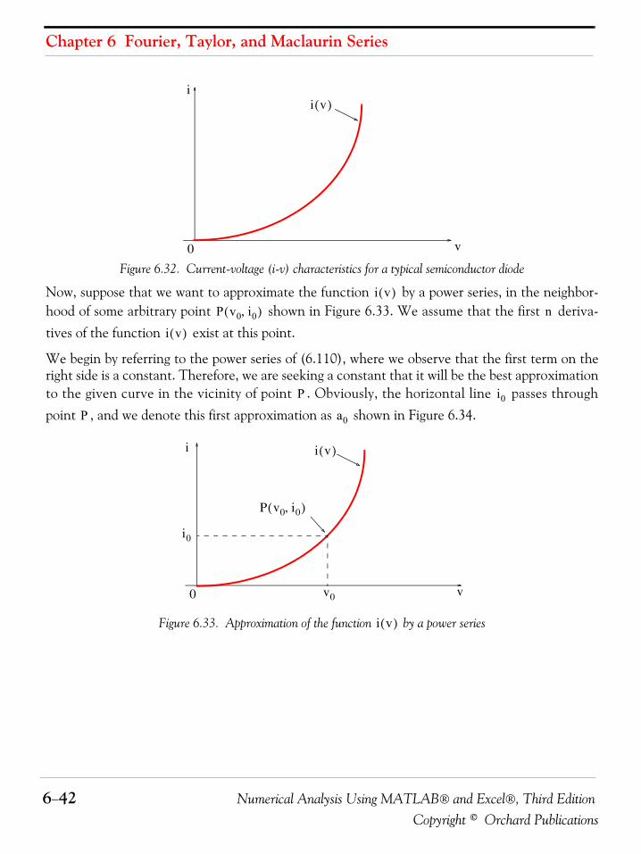
Chapter 6 Fourier, Taylor, and Maclaurin Series
6−42 Numerical Analysis Using MATLAB® and Excel®, Third EditionCopyright © Orchard Publications
Figure 6.32. Current-voltage (i-v) characteristics for a typical semiconductor diode
Now, suppose that we want to approximate the function by a power series, in the neighbor-hood of some arbitrary point shown in Figure 6.33. We assume that the first deriva-tives of the function exist at this point.
We begin by referring to the power series of (6.110), where we observe that the first term on theright side is a constant. Therefore, we are seeking a constant that it will be the best approximationto the given curve in the vicinity of point . Obviously, the horizontal line passes throughpoint , and we denote this first approximation as shown in Figure 6.34.
Figure 6.33. Approximation of the function by a power series
v
i
0
i v( )
i v( )P v0 i0,( ) n
i v( )
P i0
P a0
v
i
0
i v( )
P v0 i0,( )
v0
i0
i v( )
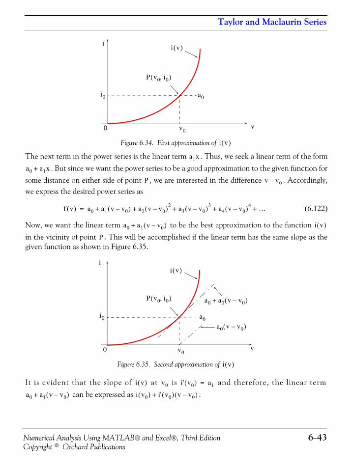
Numerical Analysis Using MATLAB® and Excel®, Third Edition 6−43Copyright © Orchard Publications
Taylor and Maclaurin Series
Figure 6.34. First approximation of
The next term in the power series is the linear term . Thus, we seek a linear term of the form. But since we want the power series to be a good approximation to the given function for
some distance on either side of point , we are interested in the difference . Accordingly,we express the desired power series as
(6.122)
Now, we want the linear term to be the best approximation to the function in the vicinity of point . This will be accomplished if the linear term has the same slope as thegiven function as shown in Figure 6.35.
Figure 6.35. Second approximation of
It is evident that the slope of at is and therefore, the linear term can be expressed as .
v
i
0
i v( )
P v0 i0,( )
i0
v0
a0
i v( )
a1x
a0 a1x+
P v v0–
f v( ) a0 a1 v v0–( ) a2 v v0–( )2 a3 v v0–( )3 a4 v v0–( )4 …+ + + + +=
a0 a1 v v0–( )+ i v( )
P
v
i
0 v0
i0 a0
i v( )
P v0 i0,( )
a0 v v0–( )
a0 a0 v v0–( )+
i v( )
i v( ) v0 i' v0( ) a1=
a0 a1 v v0–( )+ i v0( ) i' v0( ) v v0–( )+
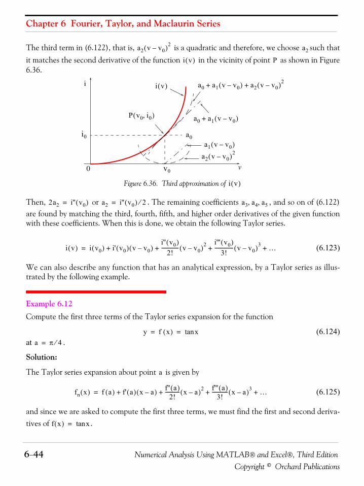
Chapter 6 Fourier, Taylor, and Maclaurin Series
6−44 Numerical Analysis Using MATLAB® and Excel®, Third EditionCopyright © Orchard Publications
The third term in (6.122), that is, is a quadratic and therefore, we choose such thatit matches the second derivative of the function in the vicinity of point as shown in Figure6.36.
Figure 6.36. Third approximation of
Then, or . The remaining coefficients , and so on of (6.122)are found by matching the third, fourth, fifth, and higher order derivatives of the given functionwith these coefficients. When this is done, we obtain the following Taylor series.
(6.123)
We can also describe any function that has an analytical expression, by a Taylor series as illus-trated by the following example.
Example 6.12 Compute the first three terms of the Taylor series expansion for the function
(6.124)at .
Solution:
The Taylor series expansion about point is given by
(6.125)
and since we are asked to compute the first three terms, we must find the first and second deriva-tives of .
a2 v v0–( )2 a2
i v( ) P
v
i
0
i v( )
P v0 i0,( ) a0 a1 v v0–( )+
a0a1 v v0–( )
i0
v0
a0 a1 v v0–( ) a2 v v0–( )2+ +
a2 v v0–( )2
i v( )
2a2 i'' v0( )= a2 i'' v0( ) 2⁄= a3 a4 a5, ,
i v( ) i v0( ) i' v0( ) v v0–( )i'' v0( )
2!-------------- v v0–( )2 i''' v0( )
3!--------------- v v0–( )3 …+ + + +=
y f x( ) xtan= =
a π 4⁄=
a
fn x( ) f a( ) f' a( ) x a–( ) f'' a( )2!
------------ x a–( )2 f''' a( )3!
------------- x a–( )3 …+ + + +=
f x( ) xtan=
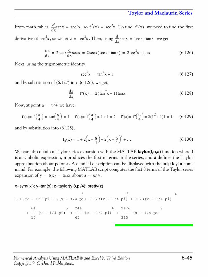
Numerical Analysis Using MATLAB® and Excel®, Third Edition 6−45Copyright © Orchard Publications
Taylor and Maclaurin Series
From math tables, , so . To find we need to find the first
derivative of , so we let . Then, using , we get
(6.126)
Next, using the trigonometric identity
(6.127)
and by substitution of (6.127) into (6.126), we get,
(6.128)
Now, at point we have:
(6.129)
and by substitution into (6.125),
(6.130)
We can also obtain a Taylor series expansion with the MATLAB taylor(f,n,a) function where fis a symbolic expression, n produces the first terms in the series, and a defines the Taylorapproximation about point . A detailed description can be displayed with the help taylor com-mand. For example, the following MATLAB script computes the first 8 terms of the Taylor seriesexpansion of about .
x=sym('x'); y=tan(x); z=taylor(y,8,pi/4); pretty(z)
2 3 41 + 2x - 1/2 pi + 2(x - 1/4 pi) + 8/3(x - 1/4 pi) + 10/3(x - 1/4 pi)
64 5 244 6 2176 7 + -- (x - 1/4 pi) + --- (x - 1/4 pi) + ---- (x - 1/4 pi) 15 45 315
xdd xtan x2sec= f ′ x( ) x2sec= f'' x( )
x2sec z x2sec=d
dx------ xsec x xtan⋅sec=
dzdx------ 2 xsec d
dx------ xsec 2 x x xtan⋅sec( )sec 2 x2 xtan⋅sec= = =
x2sec x2tan 1+=
dzdx------ f'' x( ) 2 x2tan 1+( ) xtan= =
a π 4⁄=
f a( ) f π4---⎝ ⎠
⎛ ⎞= π4---⎝ ⎠
⎛ ⎞tan 1 f' a( ) f' π4---⎝ ⎠
⎛ ⎞= 1 1+ 2 f'' a( ) f'' π4---⎝ ⎠
⎛ ⎞= 2 12 1+( )1 4= == == =
fn x( ) 1 2 x π4---–⎝ ⎠
⎛ ⎞ 2 x π4---–⎝ ⎠
⎛ ⎞ 2+ += …+
na
y f x( ) xtan= = a π 4⁄=
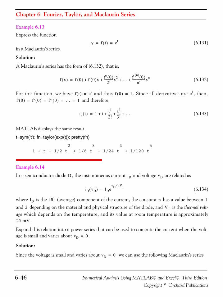
Chapter 6 Fourier, Taylor, and Maclaurin Series
6−46 Numerical Analysis Using MATLAB® and Excel®, Third EditionCopyright © Orchard Publications
Example 6.13 Express the function
(6.131)in a Maclaurin’s series.
Solution:
A Maclaurin’s series has the form of (6.132), that is,
(6.132)
For this function, we have and thus . Since all derivatives are , then, and therefore,
(6.133)
MATLAB displays the same result.
t=sym('t'); fn=taylor(exp(t)); pretty(fn)
2 3 4 5 1 + t + 1/2 t + 1/6 t + 1/24 t + 1/120 t
Example 6.14
In a semiconductor diode , the instantaneous current and voltage are related as
(6.134)
where is the DC (average) component of the current, the constant has a value between and depending on the material and physical structure of the diode, and is the thermal volt-age which depends on the temperature, and its value at room temperature is approximately
.
Expand this relation into a power series that can be used to compute the current when the volt-age is small and varies about .
Solution:
Since the voltage is small and varies about , we can use the following Maclaurin’s series.
y f t( ) et= =
f x( ) f 0( ) f' 0( )x f'' 0( )2!
------------x2 … f n( ) 0( )n!
-----------------xn+ + + +=
f t( ) et= f 0( ) 1= et
f' 0( ) f'' 0( ) f''' 0( ) … 1= = = =
fn t( ) 1 t t2
2!----- t3
3!----- …+ + + +=
D iD vD
iD vD( ) IDevD nVT⁄
=
ID n 1
2 VT
25 mV
vD 0=
vD 0=
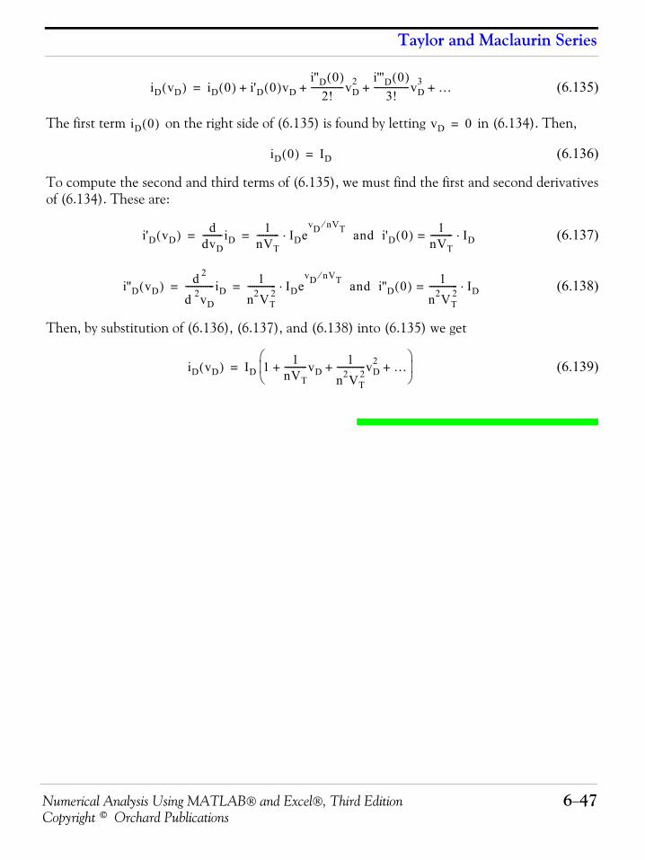
Numerical Analysis Using MATLAB® and Excel®, Third Edition 6−47Copyright © Orchard Publications
Taylor and Maclaurin Series
(6.135)
The first term on the right side of (6.135) is found by letting in (6.134). Then,
(6.136)
To compute the second and third terms of (6.135), we must find the first and second derivativesof (6.134). These are:
(6.137)
(6.138)
Then, by substitution of (6.136), (6.137), and (6.138) into (6.135) we get
(6.139)
iD vD( ) iD 0( ) i'D 0( )vDi''D 0( )
2!---------------vD
2 i'''D 0( )3!
----------------vD3 …+ + + +=
iD 0( ) vD 0=
iD 0( ) ID=
i'D vD( ) ddvD---------iD
1nVT---------- IDe
vD nVT⁄ and i'D 0( ) 1
nVT---------- ID⋅=⋅= =
i''D vD( ) d 2
d 2vD
-------------iD1
n2VT2
------------- IDevD nVT⁄
and i''D 0( ) 1n2VT
2------------- ID⋅=⋅= =
iD vD( ) ID 1 1nVT----------vD
1n2VT
2-------------vD
2 …+ + +⎝ ⎠⎜ ⎟⎛ ⎞
=
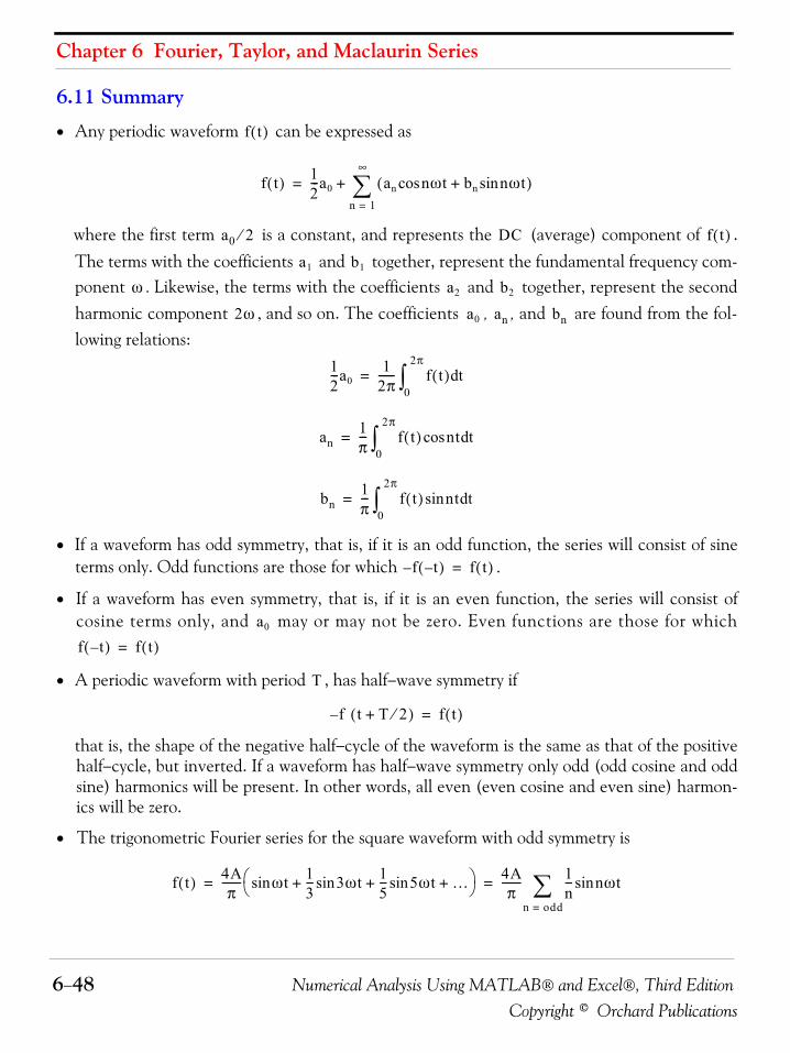
Chapter 6 Fourier, Taylor, and Maclaurin Series
6−48 Numerical Analysis Using MATLAB® and Excel®, Third EditionCopyright © Orchard Publications
6.11 Summary
• Any periodic waveform can be expressed as
where the first term is a constant, and represents the (average) component of .The terms with the coefficients and together, represent the fundamental frequency com-ponent . Likewise, the terms with the coefficients and together, represent the secondharmonic component , and so on. The coefficients , , and are found from the fol-lowing relations:
• If a waveform has odd symmetry, that is, if it is an odd function, the series will consist of sineterms only. Odd functions are those for which .
• If a waveform has even symmetry, that is, if it is an even function, the series will consist ofcosine terms only, and may or may not be zero. Even functions are those for which
• A periodic waveform with period , has half−wave symmetry if
that is, the shape of the negative half−cycle of the waveform is the same as that of the positivehalf−cycle, but inverted. If a waveform has half−wave symmetry only odd (odd cosine and oddsine) harmonics will be present. In other words, all even (even cosine and even sine) harmon-ics will be zero.
• The trigonometric Fourier series for the square waveform with odd symmetry is
f t( )
f t( ) 12---a0 an nωtcos bn nωtsin+( )
n 1=
∞
∑+=
a0 2⁄ DC f t( )
a1 b1
ω a2 b2
2ω a0 an bn
12---a0
12π------ f t( ) td
0
2π
∫=
an1π--- f t( ) nt tdcos
0
2π
∫=
bn1π--- f t( ) nt tdsin
0
2π
∫=
f t–( )– f t( )=
a0
f t–( ) f t( )=
T
f– t T 2⁄+( ) f t( )=
f t( ) 4Aπ
------- ωt 13--- 3ωt 1
5--- 5ωtsin …+ +sin+sin⎝ ⎠
⎛ ⎞ 4Aπ
------- 1n--- nωtsin
n odd=∑= =
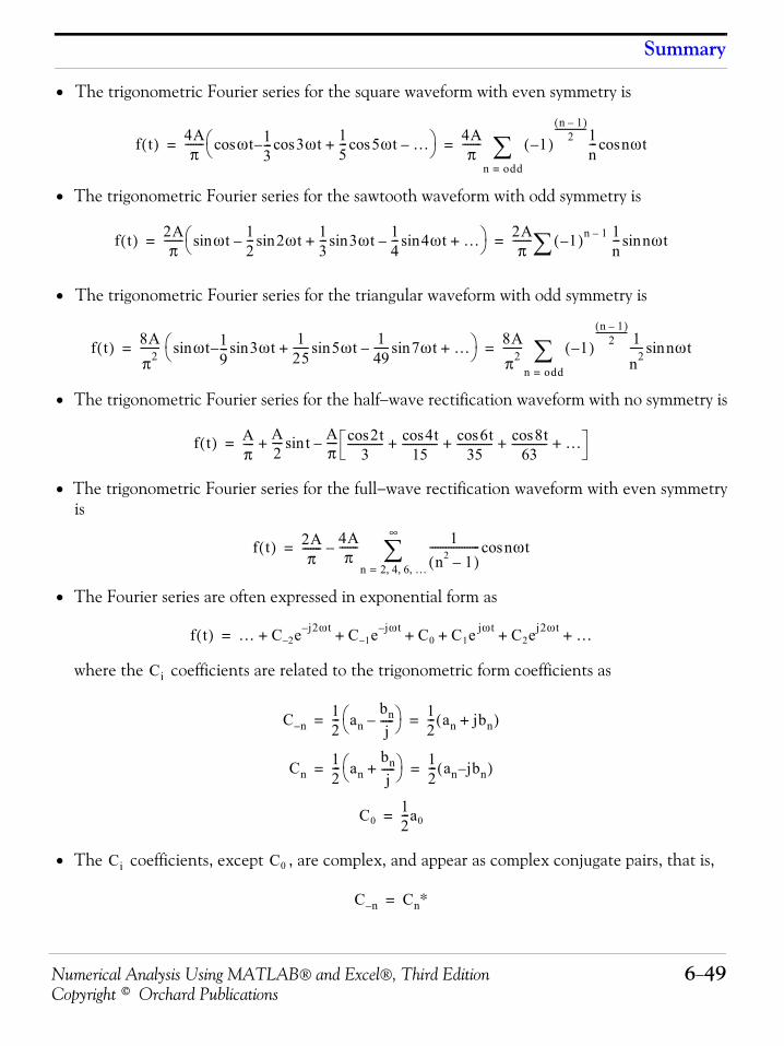
Numerical Analysis Using MATLAB® and Excel®, Third Edition 6−49Copyright © Orchard Publications
Summary
• The trigonometric Fourier series for the square waveform with even symmetry is
• The trigonometric Fourier series for the sawtooth waveform with odd symmetry is
• The trigonometric Fourier series for the triangular waveform with odd symmetry is
• The trigonometric Fourier series for the half−wave rectification waveform with no symmetry is
• The trigonometric Fourier series for the full−wave rectification waveform with even symmetryis
• The Fourier series are often expressed in exponential form as
where the coefficients are related to the trigonometric form coefficients as
• The coefficients, except , are complex, and appear as complex conjugate pairs, that is,
f t( ) 4Aπ
------- ωcos t 13---– 3ωt 1
5--- 5ωtcos …–+cos⎝ ⎠
⎛ ⎞ 4Aπ
------- 1–( )n 1–( )
2----------------1
n--- ncos ωt
n odd=∑= =
f t( ) 2Aπ
------- ωt 12--- 2ωt 1
3--- 3ωtsin 1
4--- 4ωt …+sin–+sin–sin⎝ ⎠
⎛ ⎞ 2Aπ
------- 1–( )n 1–∑1n--- nωtsin= =
f t( ) 8Aπ2------- ωsin t 1
9---– 3ωt 1
25------ 5ωtsin 1
49------ 7ωtsin …+–+sin⎝ ⎠
⎛ ⎞ 8Aπ2------- 1–( )
n 1–( )2
---------------- 1n2----- nsin ωt
n odd=∑= =
f t( ) Aπ---- A
2---- tsin A
π---- 2tcos
3------------- 4tcos
15------------- 6tcos
35------------- 8tcos
63------------- …+ + + +–+=
f t( ) 2Aπ
------- 4Aπ
------- 1n2 1–( )
------------------- nωtcosn 2 4 6 …, , ,=
∞
∑–=
f t( ) … C 2– e j2ωt– C 1– e jωt– C0 C1e jωt C2ej2ωt …+ + + + + +=
Ci
C n–12--- an
bnj
-----–⎝ ⎠⎛ ⎞ 1
2--- an jbn+( )= =
Cn12--- an
bnj
-----+⎝ ⎠⎛ ⎞ 1
2--- an j– bn( )= =
C012---a0=
Ci C0
C n– Cn∗=
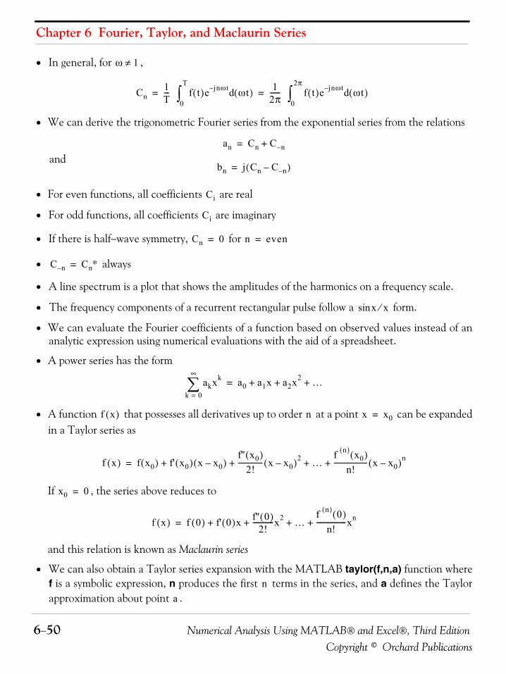
Chapter 6 Fourier, Taylor, and Maclaurin Series
6−50 Numerical Analysis Using MATLAB® and Excel®, Third EditionCopyright © Orchard Publications
• In general, for ,
• We can derive the trigonometric Fourier series from the exponential series from the relations
and
• For even functions, all coefficients are real
• For odd functions, all coefficients are imaginary
• If there is half−wave symmetry, for
• always
• A line spectrum is a plot that shows the amplitudes of the harmonics on a frequency scale.
• The frequency components of a recurrent rectangular pulse follow a form.
• We can evaluate the Fourier coefficients of a function based on observed values instead of ananalytic expression using numerical evaluations with the aid of a spreadsheet.
• A power series has the form
• A function that possesses all derivatives up to order at a point can be expandedin a Taylor series as
If , the series above reduces to
and this relation is known as Maclaurin series
• We can also obtain a Taylor series expansion with the MATLAB taylor(f,n,a) function wheref is a symbolic expression, n produces the first terms in the series, and a defines the Taylorapproximation about point .
ω 1≠
Cn1T--- f t( )e jnωt– ωt( )d
0
T
∫1
2π------ f t( )e jnωt– ωt( )d
0
2π
∫= =
an Cn C n–+=
bn j Cn C n––( )=
Ci
Ci
Cn 0= n even=
C n– Cn∗=
xsin x⁄
akxk
k 0=
∞
∑ a0 a1x a2x2 …+ + +=
f x( ) n x x0=
f x( ) f x0( ) f' x0( ) x x0–( )f'' x0( )
2!-------------- x x0–( )2 …
f n( ) x0( )n!
------------------- x x0–( )n+ + + +=
x0 0=
f x( ) f 0( ) f' 0( )x f'' 0( )2!
------------x2 …f n( ) 0( )
n!-----------------xn+ + + +=
na
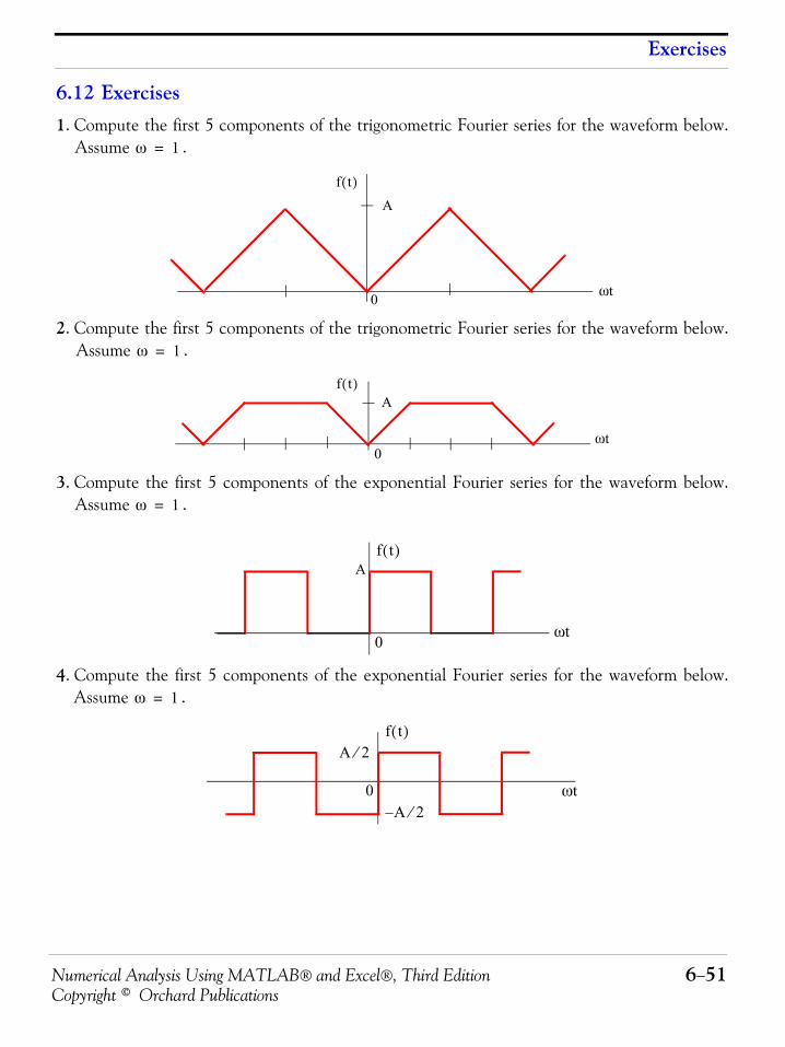
Numerical Analysis Using MATLAB® and Excel®, Third Edition 6−51Copyright © Orchard Publications
Exercises
6.12 Exercises1. Compute the first 5 components of the trigonometric Fourier series for the waveform below.
Assume .
2. Compute the first 5 components of the trigonometric Fourier series for the waveform below.Assume .
3. Compute the first 5 components of the exponential Fourier series for the waveform below.Assume .
4. Compute the first 5 components of the exponential Fourier series for the waveform below.Assume .
ω 1=
0 ωt
Af t( )
ω 1=
0ωt
Af t( )
ω 1=
0ωt
Af t( )
ω 1=
0 ωt
f t( )A 2⁄
A– 2⁄
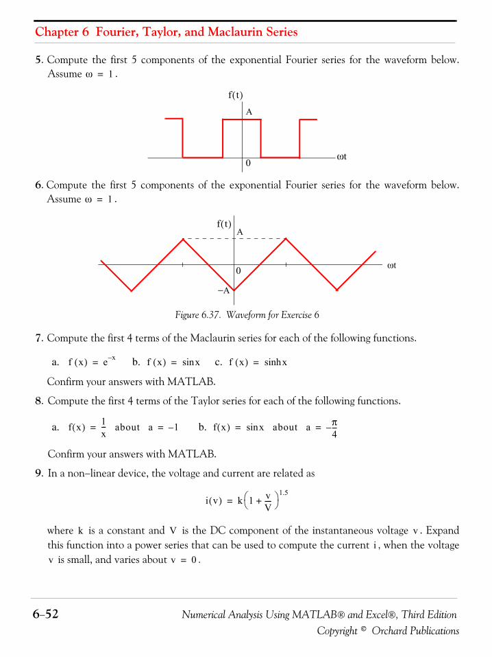
Chapter 6 Fourier, Taylor, and Maclaurin Series
6−52 Numerical Analysis Using MATLAB® and Excel®, Third EditionCopyright © Orchard Publications
5. Compute the first 5 components of the exponential Fourier series for the waveform below.Assume .
6. Compute the first 5 components of the exponential Fourier series for the waveform below.Assume .
Figure 6.37. Waveform for Exercise 6
7. Compute the first 4 terms of the Maclaurin series for each of the following functions.
a. b. c.
Confirm your answers with MATLAB.
8. Compute the first 4 terms of the Taylor series for each of the following functions.
a. b.
Confirm your answers with MATLAB.
9. In a non−linear device, the voltage and current are related as
where is a constant and is the DC component of the instantaneous voltage . Expandthis function into a power series that can be used to compute the current , when the voltage
is small, and varies about .
ω 1=
0ωt
A
f t( )
ω 1=
0 ωt
A
−A
f t( )
f x( ) e x–= f x( ) xsin= f x( ) xsinh=
f x( ) 1x--- about a 1–= = f x( ) x sin about a π
4---–= =
i v( ) k 1 vV----+⎝ ⎠
⎛ ⎞ 1.5=
k V vi
v v 0=
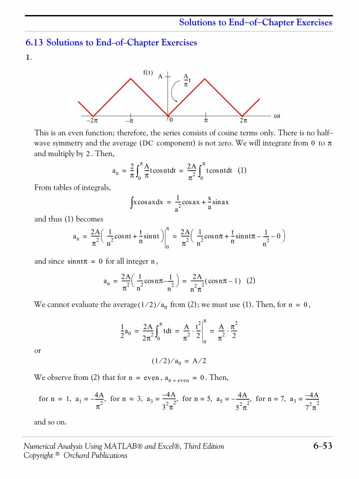
Numerical Analysis Using MATLAB® and Excel®, Third Edition 6−53Copyright © Orchard Publications
Solutions to End−of−Chapter Exercises
6.13 Solutions to End−of−Chapter Exercises1.
This is an even function; therefore, the series consists of cosine terms only. There is no half−wave symmetry and the average ( component) is not zero. We will integrate from to and multiply by . Then,
(1)
From tables of integrals,
and thus (1) becomes
and since for all integer ,
(2)
We cannot evaluate the average from (2); we must use (1). Then, for ,
or
We observe from (2) that for , . Then,
and so on.
0 ωt
Af t( ) Aπ----t
2π– π– π 2π
DC 0 π2
an2π--- A
π----t ntcos td
0
π
∫2Aπ2------- t ntcos td
0
π
∫= =
x axcos xd∫1a2----- axcos x
a--- asin x+=
an2Aπ2------- 1
n2----- ntcos t
n--- ntsin+⎝ ⎠
⎛ ⎞
0
π 2Aπ2------- 1
n2----- nπcos t
n--- ntπ 1
n2-----– 0–sin+⎝ ⎠
⎛ ⎞= =
ntπsin 0= n
an2Aπ2------- 1
n2----- nπcos 1
n2-----–⎝ ⎠
⎛ ⎞ 2A
n2π2
----------- nπ 1–cos( )= =
1 2⁄( ) a0⁄ n 0=
12---a0
2A2π2--------- t td
0
π
∫Aπ2----- t2
2----⋅
0
πAπ2----- π2
2-----⋅= = =
1 2⁄( ) a0⁄ A 2⁄=
n even= an even= 0=
for n 1 a14Aπ2-------– for n,=, 3 a3
4A–
32π2
----------- for n 5 a54A
52π2
-----------– for n,=, 7 a34A–
72π2
-----------=,= =,=,= =
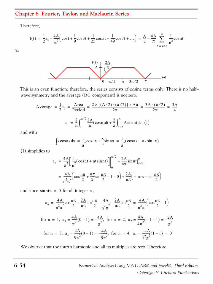
Chapter 6 Fourier, Taylor, and Maclaurin Series
6−54 Numerical Analysis Using MATLAB® and Excel®, Third EditionCopyright © Orchard Publications
Therefore,
2.
This is an even function; therefore, the series consists of cosine terms only. There is no half−wave symmetry and the average ( component) is not zero.
(1)
and with
(1) simplifies to
and since for all integer ,
We observe that the fourth harmonic and all its multiples are zero. Therefore,
f t( ) 12---a0
4Aπ2------- tcos 1
9--- 3tcos 1
25------ 5tcos 1
49------ 7tcos …+ + + +⎝ ⎠
⎛ ⎞– A2---- 4A
π------- 1
n2----- ntcos
n odd=
∞
∑–= =
0ωt
Af t( ) 2A
π-------t
ππ 2⁄ π 3π 2⁄
DC
Average 12---a0
AreaPeriod----------------- 2 A 2⁄( ) π 2⁄( )⋅[ ] Aπ+×
2π---------------------------------------------------------------- 3A π 2⁄( )⋅
2π--------------------------- 3A
4-------= = = = =
an2π--- 2A
π-------t ntcos td
0
π 2⁄
∫2π--- A ntcos td
π 2⁄
π
∫+=
x axcos xd∫1a2----- axcos x
a--- asin x+ 1
a2----- ax ax axsin+cos( )= =
an4Aπ2------- 1
n2----- ntcos nt ntsin+( )
0
π 2⁄ 2Anπ------- nt π 2⁄
πsin+=
4A
n2π2
----------- nπ2
------cos nπ2
------ nπ2
------sin 1 0––+⎝ ⎠⎛ ⎞ 2A
nπ------- nπsin nπ
2------sin–⎝ ⎠
⎛ ⎞+=
ntπsin 0= n
an4A
n2π2
----------- nπ2
------cos 2Anπ------- nπ
2------sin 4A
n2π2
-----------–2Anπ------- nπ
2------sin–+
4A
n2π2
----------- nπ2
------cos 1–⎝ ⎠⎛ ⎞= =
for n 1 a14Aπ2------- 0 1–( ) 4A
π2-------– for n,= =, 2 a2
4A4π2--------- 1– 1–( ) 2A
π2-------–= =,= =
for n 3 a34A9π2--------- 0 1–( ) 4A
9π2---------–= for n,=, 4 a4
4A–
72π2
----------- 1 1–( )=, 0= = =
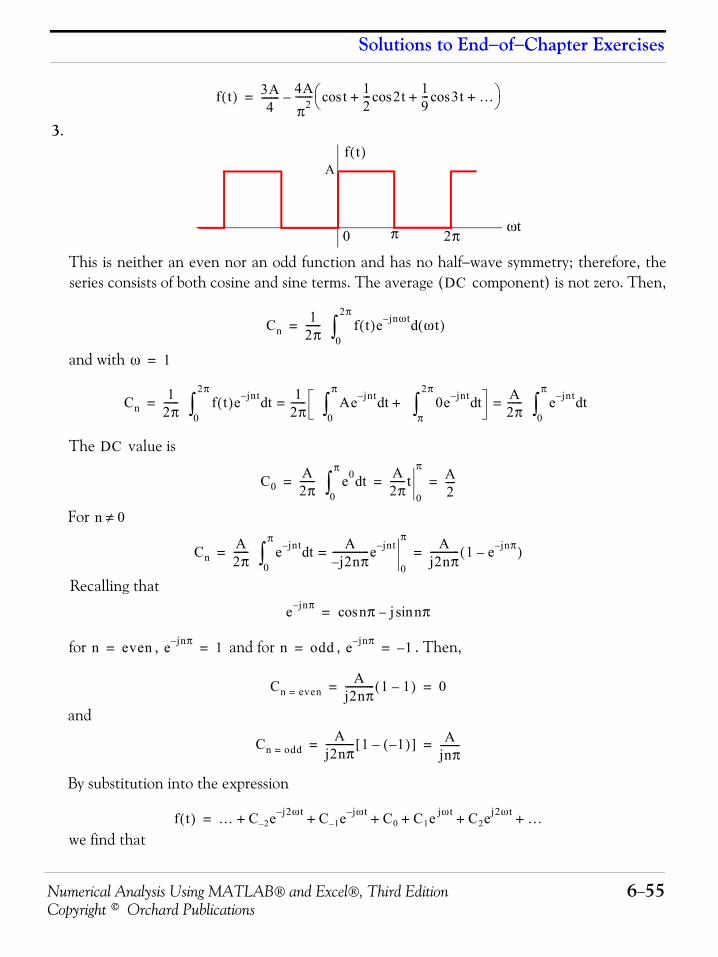
Numerical Analysis Using MATLAB® and Excel®, Third Edition 6−55Copyright © Orchard Publications
Solutions to End−of−Chapter Exercises
3.
This is neither an even nor an odd function and has no half−wave symmetry; therefore, theseries consists of both cosine and sine terms. The average ( component) is not zero. Then,
and with
The value is
For
Recalling that
for , and for , . Then,
and
By substitution into the expression
we find that
f t( ) 3A4
------- 4Aπ2------- tcos 1
2--- 2tcos 1
9--- 3tcos …+ + +⎝ ⎠
⎛ ⎞–=
0ωt
Af t( )
2ππ
DC
Cn1
2π------ f t( )e jnωt– ωt( )d
0
2π
∫=
ω 1=
Cn1
2π------ f t( )e jnt– td
0
2π
∫1
2π------ Ae jnt– td
0
π
∫ 0e jnt– tdπ
2π
∫+ A2π------ e jnt– td
0
π
∫= ==
DC
C0A2π------ e0 td
0
π
∫A2π------t
0
π A2----= = =
n 0≠
CnA2π------ e jnt– td
0
π
∫A
j2– nπ---------------e jnt–
0
π=
Aj2nπ------------ 1 e jnπ––( )= =
e jnπ– nπ j nπsin–cos=
n even= e jnπ– 1= n odd= e jnπ– 1–=
Cn even=A
j2nπ------------ 1 1–( ) 0= =
Cn odd=A
j2nπ------------ 1 1–( )–[ ] A
jnπ--------= =
f t( ) … C 2– e j2ωt– C 1– e jωt– C0 C1e jωt C2ej2ωt …+ + + + + +=
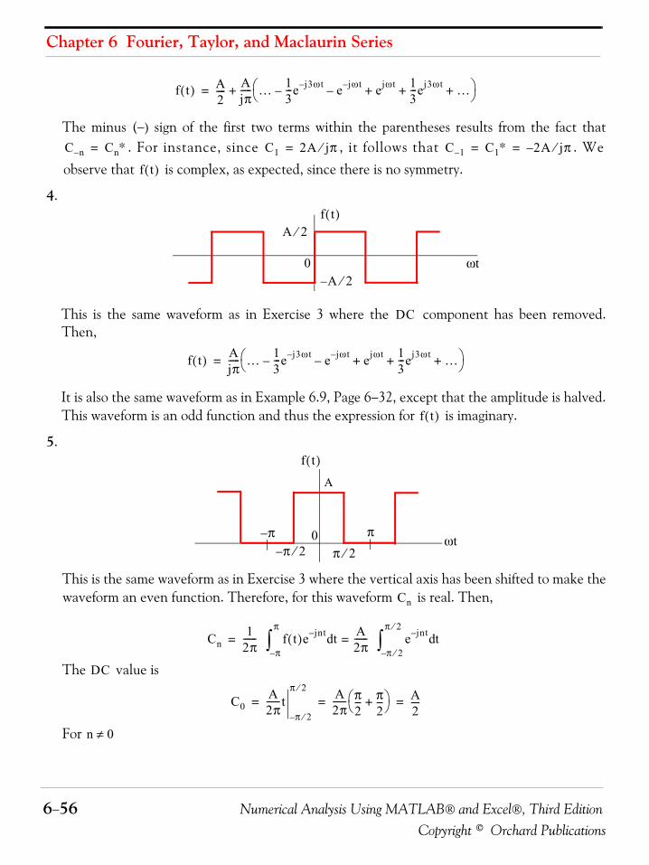
Chapter 6 Fourier, Taylor, and Maclaurin Series
6−56 Numerical Analysis Using MATLAB® and Excel®, Third EditionCopyright © Orchard Publications
The minus (−) sign of the first two terms within the parentheses results from the fact that. For instance, since , it follows that . We
observe that is complex, as expected, since there is no symmetry.
4.
This is the same waveform as in Exercise 3 where the component has been removed.Then,
It is also the same waveform as in Example 6.9, Page 6−32, except that the amplitude is halved.This waveform is an odd function and thus the expression for is imaginary.
5.
This is the same waveform as in Exercise 3 where the vertical axis has been shifted to make thewaveform an even function. Therefore, for this waveform is real. Then,
The value is
For
f t( ) A2---- A
jπ----- … 1
3---e j3ωt– e jωt––– ejωt 1
3---ej3ωt …+ + +⎝ ⎠
⎛ ⎞+=
C n– Cn∗= C1 2A jπ⁄= C 1– C1∗ 2A– jπ⁄= =
f t( )
0 ωt
f t( )A 2⁄
A– 2⁄
DC
f t( ) Ajπ----- … 1
3---e j3ωt– e jωt––– ejωt 1
3---ej3ωt …+ + +⎝ ⎠
⎛ ⎞=
f t( )
0 ωt
A
f t( )
ππ 2⁄π– 2⁄
π–
Cn
Cn1
2π------ f t( )e jnt– td
π–
π
∫A2π------ e jnt– td
π– 2⁄
π 2⁄
∫==
DC
C0A2π------t
π– 2⁄
π 2⁄ A2π------ π
2--- π
2---+⎝ ⎠
⎛ ⎞ A2----= = =
n 0≠
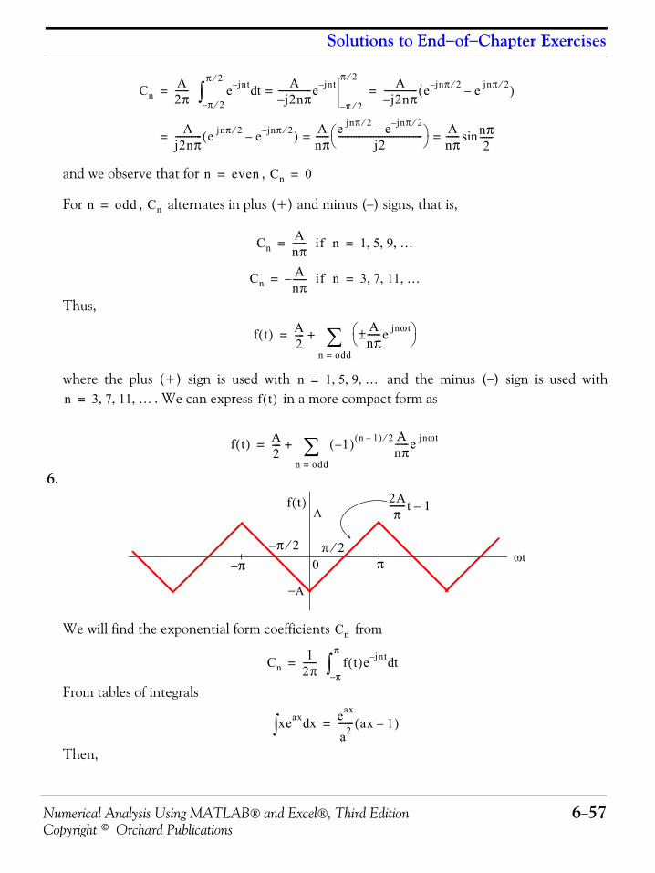
Numerical Analysis Using MATLAB® and Excel®, Third Edition 6−57Copyright © Orchard Publications
Solutions to End−of−Chapter Exercises
and we observe that for ,
For , alternates in plus (+) and minus (−) signs, that is,
Thus,
where the plus (+) sign is used with and the minus (−) sign is used with. We can express in a more compact form as
6.
We will find the exponential form coefficients from
From tables of integrals
Then,
CnA2π------ e jnt– td
π– 2⁄
π 2⁄
∫A
j2– nπ---------------e jnt–
π– 2⁄
π 2⁄= A
j2– nπ--------------- e jnπ 2⁄– e jnπ 2⁄–( )= =
Aj2nπ------------ e jnπ 2⁄ e jnπ 2⁄––( ) A
nπ------ e jnπ 2⁄ e jnπ 2⁄––
j2--------------------------------------⎝ ⎠⎛ ⎞ A
nπ------ nπ
2------sin= ==
n even= Cn 0=
n odd= Cn
CnAnπ------ if n 1 5 9 …, , ,= =
CnAnπ------– if n 3 7 11 …, , ,= =
f t( ) A2---- A
nπ------e jnωt±⎝ ⎠
⎛ ⎞
n odd=∑+=
n 1 5 9 …, , ,=
n 3 7 11 …, , ,= f t( )
f t( ) A2---- 1–( ) n 1–( ) 2⁄ A
nπ------e jnωt
n odd=∑+=
0 ωt
A
−A
f t( ) 2Aπ
-------t 1–
ππ–
π– 2⁄ π 2⁄
Cn
Cn1
2π------ f t( )e jnt– td
π–
π
∫=
xeax xd∫eax
a2------- ax 1–( )=
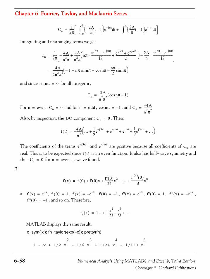
Chapter 6 Fourier, Taylor, and Maclaurin Series
6−58 Numerical Analysis Using MATLAB® and Excel®, Third EditionCopyright © Orchard Publications
Integrating and rearranging terms we get
and since for all integer ,
For , and for , , and
Also, by inspection, the component . Then,
The coefficients of the terms and are positive because all coefficients of arereal. This is to be expected since is an even function. It also has half−wave symmetry andthus for as we’ve found.
7.
a. , , , , , , ,, and so on. Therefore,
MATLAB displays the same result.
x=sym('x'); fn=taylor(exp(−x)); pretty(fn)
2 3 4 5 1 - x + 1/2 x - 1/6 x + 1/24 x - 1/120 x
Cn1
2π------ 2A
π-------– t 1–⎝ ⎠
⎛ ⎞ e jnt– tdπ–
0
∫2Aπ
-------t 1–⎝ ⎠⎛ ⎞ e jnt– td
0
π
∫+=
Cn1
2π------ 4A
n2π---------– 4A
n2π--------- nπ e jnπ e jnπ––
j2----------------------------⋅ e jnπ e jnπ–+
2----------------------------+⎝ ⎠
⎛ ⎞ 2An
------- e jnπ e jnπ––j2
----------------------------⋅–+=
4A2n2π2-------------- 1– nπ nπsin nπcos nπ
2------ nπsin–+ +⎝ ⎠
⎛ ⎞=
nπsin 0= n
Cn2A
n2π2----------- nπcos 1–( )=
n even= Cn 0= n odd= nπcos 1–= Cn4– A
n2π2-----------=
DC C0 0=
f t( ) 4Aπ2-------– … 1
9---e j3ωt– e jωt– ejωt 1
9---ej3ωt …+ + + + +⎝ ⎠
⎛ ⎞=
e j3ωt– e jωt– Cn
f t( )Cn 0= n even=
f x( ) f 0( ) f' 0( )x f'' 0( )2!
------------x2 …f n( ) 0( )
n!-----------------xn+ + + +=
f x( ) e x–= f 0( ) 1= f' x( ) e x––= f' 0( ) 1–= f'' x( ) e x–= f'' 0( ) 1= f''' x( ) e x––=
f''' 0( ) 1–=
fn x( ) 1 x– x2
2!----- x3
3!-----– …+ +=
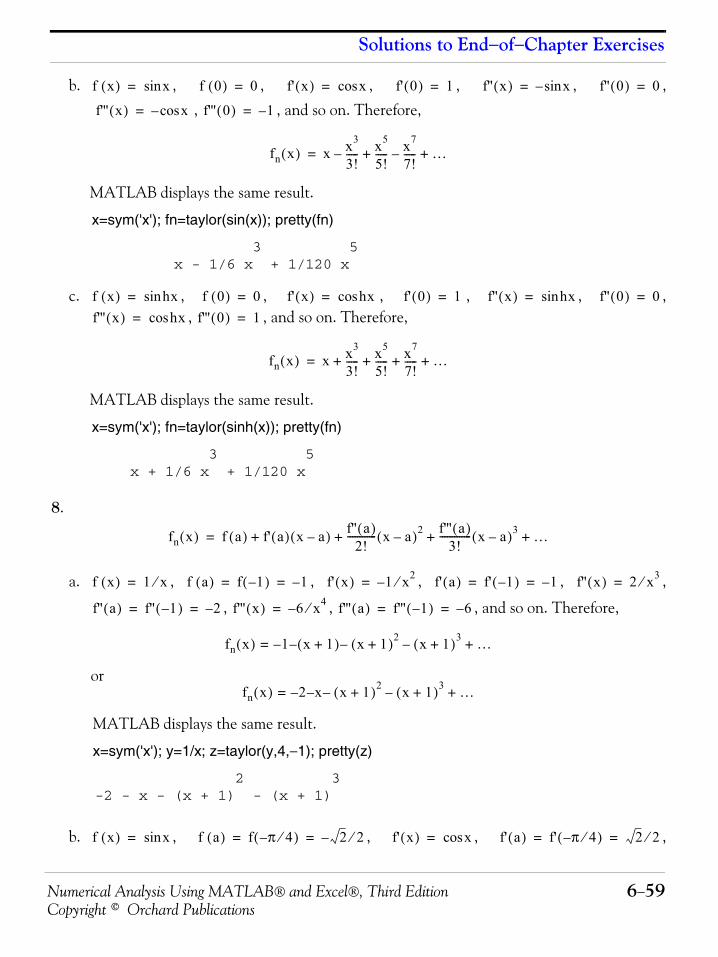
Numerical Analysis Using MATLAB® and Excel®, Third Edition 6−59Copyright © Orchard Publications
Solutions to End−of−Chapter Exercises
b. , , , , , ,
, , and so on. Therefore,
MATLAB displays the same result.
x=sym('x'); fn=taylor(sin(x)); pretty(fn)
3 5 x - 1/6 x + 1/120 x
c. , , , , , ,, , and so on. Therefore,
MATLAB displays the same result.
x=sym('x'); fn=taylor(sinh(x)); pretty(fn)
3 5 x + 1/6 x + 1/120 x
8.
a. , , , , ,
, , , and so on. Therefore,
or
MATLAB displays the same result.
x=sym('x'); y=1/x; z=taylor(y,4,−1); pretty(z)
2 3 -2 - x - (x + 1) - (x + 1)
b. , , , ,
f x( ) xsin= f 0( ) 0= f' x( ) xcos= f' 0( ) 1= f'' x( ) xsin–= f'' 0( ) 0=
f''' x( ) xcos–= f''' 0( ) 1–=
fn x( ) x x3
3!----- x5
5!----- x7
7!-----–+– …+=
f x( ) hxsin= f 0( ) 0= f' x( ) hxcos= f' 0( ) 1= f'' x( ) hxsin= f'' 0( ) 0=
f''' x( ) hxcos= f''' 0( ) 1=
fn x( ) x x3
3!----- x5
5!----- x7
7!----- …+ + + +=
fn x( ) f a( ) f' a( ) x a–( ) f'' a( )2!
------------ x a–( )2 f''' a( )3!
------------- x a–( )3 …+ + + +=
f x( ) 1 x⁄= f a( ) f 1–( ) 1–= = f' x( ) 1– x2⁄= f' a( ) f' 1–( ) 1–= = f'' x( ) 2 x3⁄=
f'' a( ) f'' 1–( ) 2–= = f''' x( ) 6– x4⁄= f''' a( ) f''' 1–( ) 6–= =
fn x( ) 1– x 1+( )– x 1+( )2– x 1+( )3–= …+
fn x( ) 2– x– x 1+( )2– x 1+( )3–= …+
f x( ) xsin= f a( ) f π 4⁄–( ) 2 2⁄–= = f' x( ) xcos= f' a( ) f' π 4⁄–( ) 2 2⁄= =
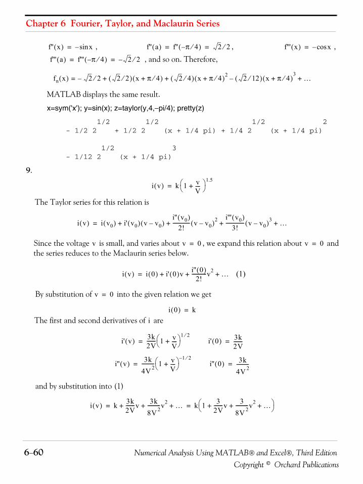
Chapter 6 Fourier, Taylor, and Maclaurin Series
6−60 Numerical Analysis Using MATLAB® and Excel®, Third EditionCopyright © Orchard Publications
, , ,
, and so on. Therefore,
MATLAB displays the same result.
x=sym('x'); y=sin(x); z=taylor(y,4,−pi/4); pretty(z)
1/2 1/2 1/2 2 - 1/2 2 + 1/2 2 (x + 1/4 pi) + 1/4 2 (x + 1/4 pi)
1/2 3 - 1/12 2 (x + 1/4 pi)
9.
The Taylor series for this relation is
Since the voltage is small, and varies about , we expand this relation about andthe series reduces to the Maclaurin series below.
(1)
By substitution of into the given relation we get
The first and second derivatives of are
and by substitution into (1)
f'' x( ) xsin–= f'' a( ) f'' π 4⁄–( ) 2 2⁄= = f''' x( ) xcos–=
f''' a( ) f''' π 4⁄–( ) 2 2⁄–= =
fn x( ) 2 2⁄– 2 2⁄( )+ x π 4⁄+( ) 2 4⁄( )+ x π 4⁄+( )2 2 12⁄( ) x π 4⁄+( )3
–= …+
i v( ) k 1 vV----+⎝ ⎠
⎛ ⎞ 1.5=
i v( ) i v0( ) i' v0( ) v v0–( )i'' v0( )
2!-------------- v v0–( )2 i''' v0( )
3!--------------- v v0–( )3 …+ + + +=
v v 0= v 0=
i v( ) i 0( ) i' 0( )v i'' 0( )2!
------------v2 …+ + +=
v 0=
i 0( ) k=
i
i' v( ) 3k2V------- 1 v
V----+⎝ ⎠
⎛ ⎞ 1 2⁄= i' 0( ) 3k
2V-------=
i'' v( ) 3k4V 2---------- 1 v
V----+⎝ ⎠
⎛ ⎞ 1 2⁄–= i'' 0( ) 3k
4V 2----------=
i v( ) k 3k2V-------v 3k
8V 2----------v2 …+ + + k 1 3
2V-------v 3
8V 2----------v2 …+ + +⎝ ⎠
⎛ ⎞= =
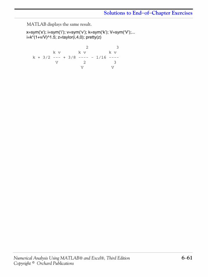
Numerical Analysis Using MATLAB® and Excel®, Third Edition 6−61Copyright © Orchard Publications
Solutions to End−of−Chapter Exercises
MATLAB displays the same result.
x=sym('x'); i=sym(‘i’); v=sym(‘v’); k=sym(‘k’); V=sym(‘V’);...i=k*(1+v/V)^1.5; z=taylor(i,4,0); pretty(z)
2 3 k v k v k v k + 3/2 --- + 3/8 ---- - 1/16 ---- V 2 3 V V
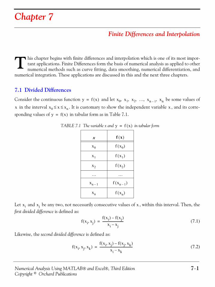
Numerical Analysis Using MATLAB® and Excel®, Third Edition 7−1Copyright © Orchard Publications
Chapter 7
Finite Differences and Interpolation
his chapter begins with finite differences and interpolation which is one of its most impor-tant applications. Finite Differences form the basis of numerical analysis as applied to othernumerical methods such as curve fitting, data smoothing, numerical differentiation, and
numerical integration. These applications are discussed in this and the next three chapters.
7.1 Divided Differences
Consider the continuous function and let be some values of
in the interval . It is customary to show the independent variable , and its corre-sponding values of in tabular form as in Table 7.1.
Let and be any two, not necessarily consecutive values of , within this interval. Then, thefirst divided difference is defined as:
(7.1)
Likewise, the second divided difference is defined as:
(7.2)
TABLE 7.1 The variable x and in tabular form
x
… …
T
y f x( )= x0 x1 x2 … xn 1– xn, , , , ,
x x0 x xn≤ ≤ x
y f x( )=
y f x( )=
f x( )
x0 f x0( )
x1 f x1( )
x2 f x2( )
xn 1– f xn 1–( )
xn f xn( )
xi xj x
f xi xj,( )f xi( ) f xj( )–
xi xj–-----------------------------=
f xi xj xk, ,( )f xi xj,( ) f xj xk,( )–
xi xk–---------------------------------------------=
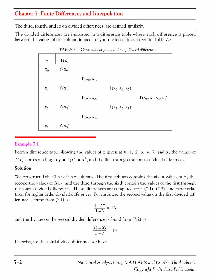
Chapter 7 Finite Differences and Interpolation
7−2 Numerical Analysis Using MATLAB® and Excel®, Third EditionCopyright © Orchard Publications
The third, fourth, and so on divided differences, are defined similarly.
The divided differences are indicated in a difference table where each difference is placedbetween the values of the column immediately to the left of it as shown in Table 7.2.
Example 7.1
Form a difference table showing the values of given as , the values of
corresponding to , and the first through the fourth divided differences.
Solution:
We construct Table 7.3 with six columns. The first column contains the given values of , thesecond the values of , and the third through the sixth contain the values of the first throughthe fourth divided differences. These differences are computed from (7.1), (7.2), and other rela-tions for higher order divided differences. For instance, the second value on the first divided dif-ference is found from (7.1) as
and third value on the second divided difference is found from (7.2) as
Likewise, for the third divided difference we have
TABLE 7.2 Conventional presentation of divided differences
x f x( )
x0 f x0( )
f x0 x1,( )
x1 f x1( ) f x0 x1 x2, ,( )
f x1 x2,( ) f x0 x1 x2 x3, , ,( )
x2 f x2( ) f x1 x2 x3, ,( )
f x2 x3,( )
x3 f x3( )
x 0 1 2 3 4 7 and 9, , , , , ,
f x( ) y f x( ) x3= =
xf x( )
1 27–1 3–--------------- 13=
37 93–3 7–
------------------ 14=
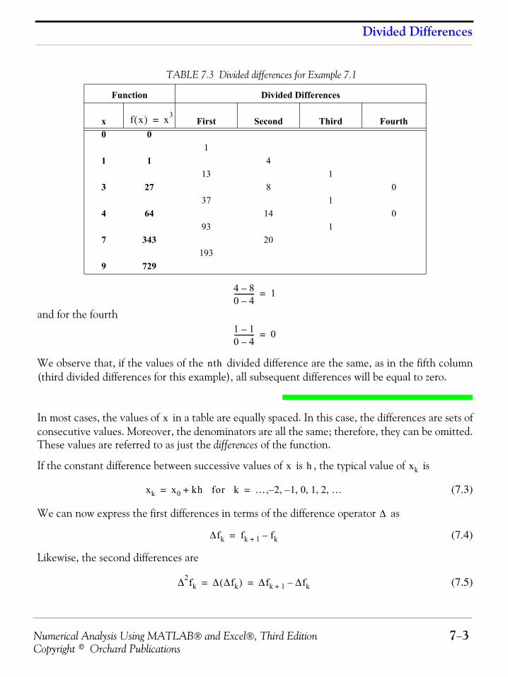
Numerical Analysis Using MATLAB® and Excel®, Third Edition 7−3Copyright © Orchard Publications
Divided Differences
and for the fourth
We observe that, if the values of the divided difference are the same, as in the fifth column(third divided differences for this example), all subsequent differences will be equal to zero.
In most cases, the values of in a table are equally spaced. In this case, the differences are sets ofconsecutive values. Moreover, the denominators are all the same; therefore, they can be omitted.These values are referred to as just the differences of the function.
If the constant difference between successive values of is , the typical value of is
(7.3)
We can now express the first differences in terms of the difference operator as
(7.4)
Likewise, the second differences are
(7.5)
TABLE 7.3 Divided differences for Example 7.1
Function Divided Differences
x First Second Third Fourth0 0
11 1 4
13 13 27 8 0
37 14 64 14 0
93 17 343 20
1939 729
f x( ) x3=
4 8–0 4–------------ 1=
1 1–0 4–------------ 0=
nth
x
x h xk
xk x0 kh for k+ … 2 1 0 1 2 …, , , ,–,–,= =
Δ
Δfk fk 1+ fk–=
Δ2fk Δ Δfk( ) Δfk 1+ Δfk–= =
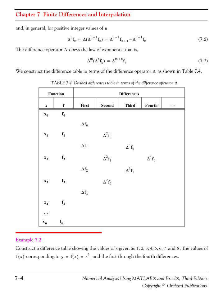
Chapter 7 Finite Differences and Interpolation
7−4 Numerical Analysis Using MATLAB® and Excel®, Third EditionCopyright © Orchard Publications
and, in general, for positive integer values of
(7.6)
The difference operator obeys the law of exponents, that is,
(7.7)
We construct the difference table in terms of the difference operator as shown in Table 7.4.
Example 7.2
Construct a difference table showing the values of x given as and , the values of
corresponding to , and the first through the fourth differences.
TABLE 7.4 Divided differences table in terms of the difference operator
Function Differences
x f First Second Third Fourth
n
Δnfk Δ Δn 1– fk( ) Δn 1– fk 1+ Δn 1– fk–= =
Δ
Δm Δnfk( ) Δm n+ fk=
Δ
Δ
…
x0 f0
Δf0
x1 f1 Δ2f0
Δf1 Δ3f0
x2 f2 Δ2f1 Δ4f0
Δf2 Δ3f1
x3 f3 Δ2f2
Δf3
x4 f4
…
xn fn
1 2 3 4 5 6 7, , , , , , 8
f x( ) y f x( ) x3= =
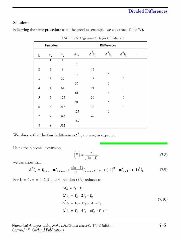
Numerical Analysis Using MATLAB® and Excel®, Third Edition 7−5Copyright © Orchard Publications
Divided Differences
Solution:
Following the same procedure as in the previous example, we construct Table 7.5.
We observe that the fourth differences are zero, as expected.
Using the binomial expansion
(7.8)
we can show that
(7.9)
For , and , relation (7.9) reduces to
(7.10)
TABLE 7.5 Difference table for Example 7.2
Function Differences
k xk fk
1 1 17
2 2 8 1219 6
3 3 27 18 037 6
4 4 64 24 061 6
5 5 125 30 091 6
6 6 216 36 0127 6
7 7 343 42169
8 8 512
Δfk Δ2fk Δ3fk Δ4fk …
Δ4fk
nj⎝ ⎠
⎛ ⎞ n!j! n j–( )!---------------------=
Δnfk fk n+ nfk n 1–+–n n 1–( )
2!--------------------fk n 2–+ … 1–( )n 1– nfk 1+ 1–( )nfk+ + + +=
k 0= n 1 2 3, ,= 4
Δf0 f2 f1–=
Δ2f0 f2 2f1– f0+=
Δ3f0 f3 3f2– 3f1 f0–+=
Δ4f0 f4 4f3 6f2 4– f1 f0+ +–=
Chapter 7 Finite Differences and Interpolation
7−6 Numerical Analysis Using MATLAB® and Excel®, Third EditionCopyright © Orchard Publications
It is interesting to observe that the first difference in (7.10), is the difference quotient whose limitdefines the derivative of a continuous function that is defined as
(7.11)
As with derivatives, the differences of a polynomial of degree are constant.
7.2 Factorial PolynomialsThe factorial polynomials are defined as
(7.12)and
(7.13)
These expressions resemble the power functions and in elementary algebra.
Using the difference operator with (7.12) and (7.13) we obtain
(7.14)and
(7.15)
We observe that (7.14) and (7.15) are very similar to differentiation of and .
Occasionally, it is desirable to express a polynomial as a factorial polynomial. Then, in anal-ogy with Maclaurin power series, we can express that polynomial as
(7.16)
and now our task is to compute the coefficients .For , relation (7.16) reduces to
(7.17)
To compute the coefficient , we take the first difference of in (7.16). Using (7.14) weobtain
(7.18)
and letting , we find that
ΔyΔx-------
Δx 0→lim
f x1 Δx+( ) f x1( )–
Δx--------------------------------------------
Δx 0→lim=
nth n
x( ) n( ) x x 1–( ) x 2–( )… x n– 1+( )=
x( ) n( )– 1x 1–( ) x 2–( )… x n+( )
----------------------------------------------------------=
xn x n–
Δ
Δ x( ) n( ) n x( ) n 1–( )=
Δ x( ) n( )– n– x( ) n 1–( )–=
xn x n–
pn x( )
pn x( ) a0 a1 x( ) 1( ) a2 x( ) 2( ) … an x( ) n( )+ + + +=
ak
x 0=
a0 pn 0( )=
a1 pn x( )
Δpn x( ) 1x0a1 2a2 x( ) 1( ) 3a3 x( ) 2( ) … nan x( ) n 1–( )+ + + +=
x 0=
Numerical Analysis Using MATLAB® and Excel®, Third Edition 7−7Copyright © Orchard Publications
Factorial Polynomials
(7.19)
Differencing again we obtain
(7.20)
and for ,
(7.21)
In general,
(7.22)
Factorial polynomials provide an easier method of constructing a difference table. With thismethod we perform the following steps:
1. We divide in (7.16) by to obtain a quotient and a remainder which turns out
to be the constant term . Then, we express (7.16) as
(7.23)
2. We divide in (7.23) by to obtain a quotient and a remainder whichturns out to be the constant term . Then,
(7.24)
By substitution of (7.24) into (7.23), and using the form of relation (7.16), we obtain
(7.25)
3. We divide in (7.25) by to obtain a quotient and a remainder whichturns out to be the constant term , and thus
(7.26)
By substitution of (7.26) into (7.25), we obtain
(7.27)
a1 Δpn 0( )=
Δ2pn x( ) 2 1a2⋅ 3 2a⋅ 3 x( ) 1( ) … n n 1–( )an x( ) n 2–( )+ + +=
x 0=
a2Δ2pn 0( )
2 1⋅--------------------
Δ2pn 0( )2!
--------------------= =
ajΔjpn 0( )
j!------------------- for j 0 1 2 … n, , , ,= =
pn x( ) x q0 x( ) r0
a0
pn x( ) r0 xq0 x( )+=
q0 x( ) x 1–( ) q1 x( ) r1
a1
q0 x( ) r1 x 1–( )q1 x( )+=
pn x( ) r0 x r1 x 1–( )q1 x( )+[ ]+ r0 r1 x( ) 1( ) x x 1–( )q1 x( )+ += =
q1 x( ) x 2–( ) q2 x( ) r2
a2
q1 x( ) r2 x 2–( )q2 x( )+=
pn x( ) r0 r1 x( ) 1( ) x x 1–( ) r2 x 2–( )q2 x( )+[ ]+ +=
r0 r1 x( ) 1( )+ r2 x( ) 2( ) x x 1–( ) x 2–( )q2 x( )+ +=
Chapter 7 Finite Differences and Interpolation
7−8 Numerical Analysis Using MATLAB® and Excel®, Third EditionCopyright © Orchard Publications
Continuing with the above procedure, we obtain a new quotient whose degree is one less thanpreceding quotient and therefore, the process of finding new quotients and remainders terminatesafter steps.
The general form of a factorial polynomial is
(7.28)
and from (7.16) and (7.22),
(7.29)
or
(7.30)
Example 7.3 Express the algebraic polynomial
(7.31)
as a factorial polynomial. Then, construct the difference table with .
Solution:
Since the highest power of the given polynomial is , we must evaluate the remainders and ; then, we will use (7.28) to determine . We can compute the remainders
by long division, but for convenience, we will use the MATLAB deconv(p,q) function whichdivides the polynomial p by q.
The MATLAB script is as follows:
px=[1 −5 0 3 4]; % Coefficients of given polynomiald0=[1 0]; % Coefficients of first divisor, i.e, x[q0,r0]=deconv(px,d0) % Computation of first quotient and remainderd1=[1 −1]; % Coefficients of second divisor, i.e, x−1[q1,r1]=deconv(q0,d1) % Computation of second quotient and remainderd2=[1 −2]; % Coefficients of third divisor, i.e, x−2[q2,r2]=deconv(q1,d2) % Computation of third quotient and remainderd3=[1 −3]; % Coefficients of fourth divisor, i.e, x−3[q3,r3]=deconv(q2,d3) % Computation of fourth quotient and remainderd4=[1 −4]; % Coefficients of fifth (last) divisor, i.e, x−4[q4,r4]=deconv(q3,d4) % Computation of fifth (last) quotient and remainder
q0 =
n 1+( )
pn x( ) r0 r1 x( ) 1( )+ r2 x( ) 2( ) … rn 1– x( ) n 1–( ) rn x( ) n( )+ + + +=
rj ajΔjpn 0( )
j!-------------------= =
Δjpn 0( ) j!rj=
p x( ) x4 5x3– 3x 4+ +=
h 1=
p x( ) 4r0 r1 r2 r3, , , r4 pn x( )
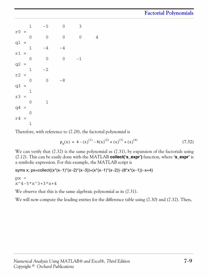
Numerical Analysis Using MATLAB® and Excel®, Third Edition 7−9Copyright © Orchard Publications
Factorial Polynomials
1 -5 0 3r0 = 0 0 0 0 4q1 = 1 -4 -4r1 = 0 0 0 -1q2 = 1 -2r2 = 0 0 -8q3 = 1r3 = 0 1q4 = 0r4 = 1
Therefore, with reference to (7.28), the factorial polynomial is
(7.32)
We can verify that (7.32) is the same polynomial as (7.31), by expansion of the factorials using(7.12). This can be easily done with the MATLAB collect(‘s_expr’) function, where ‘s_expr’ isa symbolic expression. For this example, the MATLAB script is
syms x; px=collect((x*(x−1)*(x−2)*(x−3))+(x*(x−1)*(x−2))−(8*x*(x−1))−x+4)
px =x^4-5*x^3+3*x+4
We observe that this is the same algebraic polynomial as in (7.31).
We will now compute the leading entries for the difference table using (7.30) and (7.32). Then,
pn x( ) 4 x( ) 1( )– 8 x( ) 2( )– x( ) 3( ) x( ) 4( )+ +=
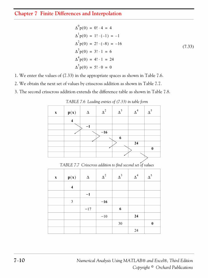
Chapter 7 Finite Differences and Interpolation
7−10 Numerical Analysis Using MATLAB® and Excel®, Third EditionCopyright © Orchard Publications
(7.33)
1. We enter the values of (7.33) in the appropriate spaces as shown in Table 7.6.
2. We obtain the next set of values by crisscross addition as shown in Table 7.7.
3. The second crisscross addition extends the difference table as shown in Table 7.8.
TABLE 7.6 Leading entries of (7.33) in table form
4−1
−166
240
TABLE 7.7 Crisscross addition to find second set of values
4
−1
3 −16
−17 6
−10 24
30 0
24
Δ0p 0( ) 0! 4⋅ 4= =
Δ1p 0( ) 1! 1–( )⋅ 1–= =
Δ2p 0( ) 2! 8–( )⋅ 16–= =
Δ3p 0( ) 3! 1⋅ 6= =
Δ4p 0( ) 4! 1⋅ 24= =
Δ5p 0( ) 5! 0⋅ 0= =
x p x( ) Δ Δ2 Δ3 Δ4 Δ5
x p x( ) Δ Δ2 Δ3 Δ4 Δ5
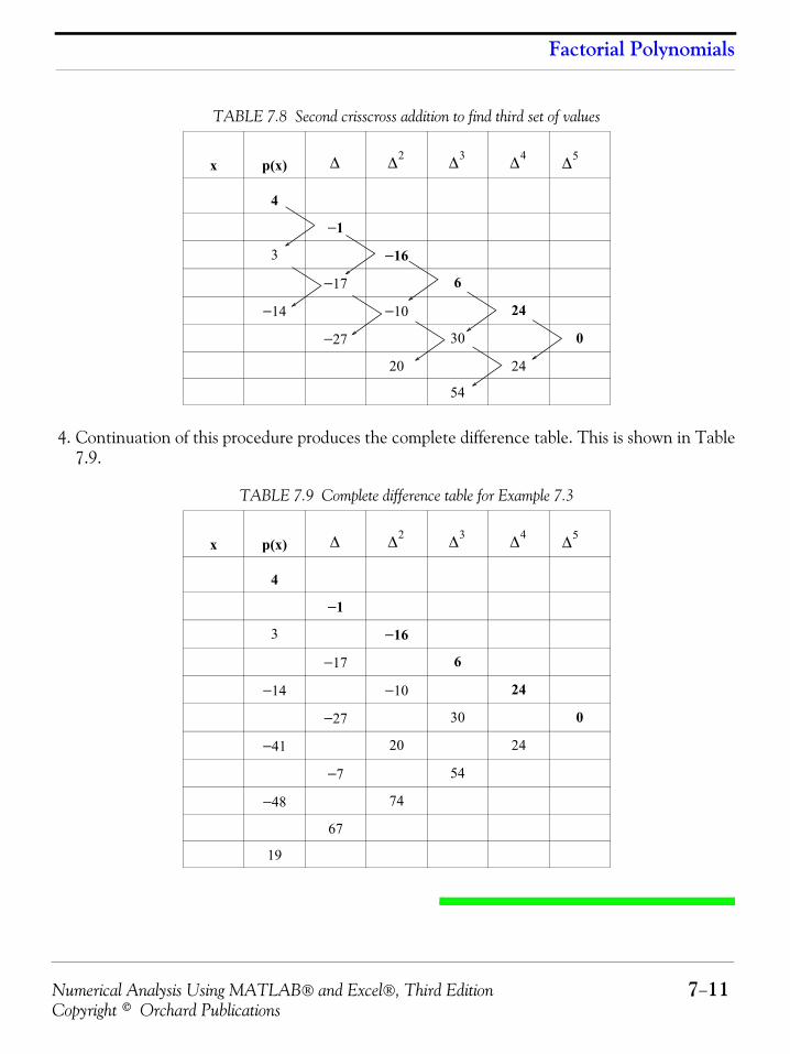
Numerical Analysis Using MATLAB® and Excel®, Third Edition 7−11Copyright © Orchard Publications
Factorial Polynomials
4. Continuation of this procedure produces the complete difference table. This is shown in Table7.9.
TABLE 7.8 Second crisscross addition to find third set of values
x p(x)
4
−1
3 −16
−17 6
−14 −10 24
−27 30 0
20 24
54
TABLE 7.9 Complete difference table for Example 7.3
x p(x)
4
−1
3 −16
−17 6
−14 −10 24
−27 30 0
−41 20 24
−7 54
−48 74
67
19
Δ Δ2 Δ3 Δ4 Δ5
Δ Δ2 Δ3 Δ4 Δ5
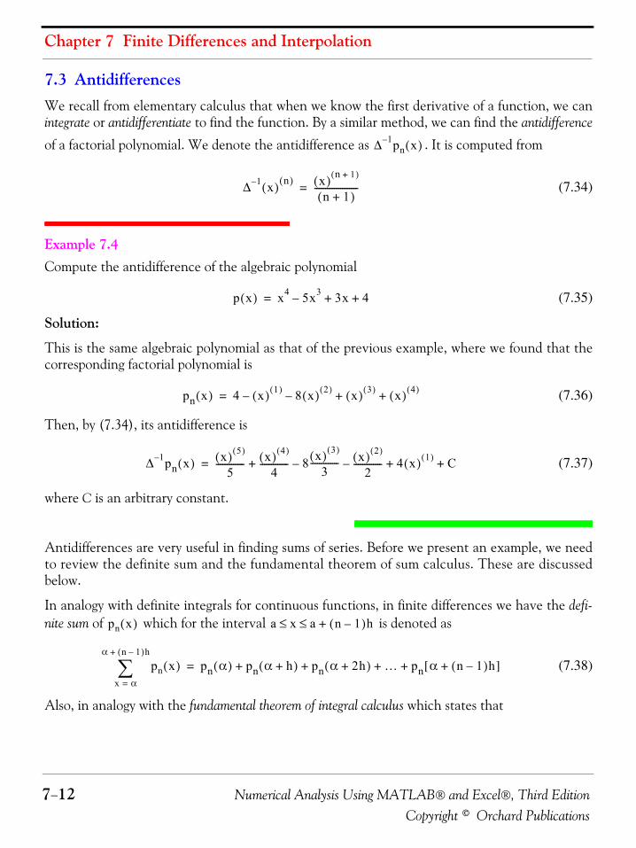
Chapter 7 Finite Differences and Interpolation
7−12 Numerical Analysis Using MATLAB® and Excel®, Third EditionCopyright © Orchard Publications
7.3 AntidifferencesWe recall from elementary calculus that when we know the first derivative of a function, we canintegrate or antidifferentiate to find the function. By a similar method, we can find the antidifference
of a factorial polynomial. We denote the antidifference as . It is computed from
(7.34)
Example 7.4 Compute the antidifference of the algebraic polynomial
(7.35)
Solution:
This is the same algebraic polynomial as that of the previous example, where we found that thecorresponding factorial polynomial is
(7.36)
Then, by (7.34), its antidifference is
(7.37)
where C is an arbitrary constant.
Antidifferences are very useful in finding sums of series. Before we present an example, we needto review the definite sum and the fundamental theorem of sum calculus. These are discussedbelow.
In analogy with definite integrals for continuous functions, in finite differences we have the defi-nite sum of which for the interval is denoted as
(7.38)
Also, in analogy with the fundamental theorem of integral calculus which states that
Δ 1– pn x( )
Δ 1– x( ) n( ) x( ) n 1+( )
n 1+( )--------------------=
p x( ) x4 5x3– 3x 4+ +=
pn x( ) 4 x( ) 1( )– 8 x( ) 2( )– x( ) 3( ) x( ) 4( )+ +=
Δ 1– pn x( ) x( ) 5( )
5------------- x( ) 4( )
4------------- 8 x( ) 3( )
3-------------– x( ) 2( )
2-------------– 4 x( ) 1( ) C+ + +=
pn x( ) a x a n 1–( )h+≤ ≤
pn x( )x α=
α n 1–( )h+
∑ pn α( ) pn α h+( ) pn α 2h+( ) … pn α n 1–( )h+[ ]+ + + +=
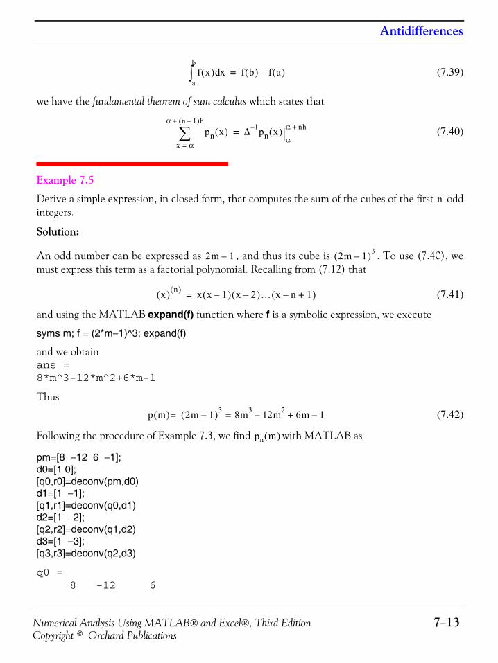
Numerical Analysis Using MATLAB® and Excel®, Third Edition 7−13Copyright © Orchard Publications
Antidifferences
(7.39)
we have the fundamental theorem of sum calculus which states that
(7.40)
Example 7.5
Derive a simple expression, in closed form, that computes the sum of the cubes of the first oddintegers.
Solution:
An odd number can be expressed as , and thus its cube is . To use (7.40), wemust express this term as a factorial polynomial. Recalling from (7.12) that
(7.41)
and using the MATLAB expand(f) function where f is a symbolic expression, we execute
syms m; f = (2*m−1)^3; expand(f)
and we obtainans =8*m^3-12*m^2+6*m-1
Thus
(7.42)
Following the procedure of Example 7.3, we find with MATLAB as
pm=[8 −12 6 −1];d0=[1 0];[q0,r0]=deconv(pm,d0)d1=[1 −1];[q1,r1]=deconv(q0,d1)d2=[1 −2];[q2,r2]=deconv(q1,d2)d3=[1 −3];[q3,r3]=deconv(q2,d3)
q0 = 8 -12 6
f x( ) xda
b
∫ f b( ) f a( )–=
pn x( )x α=
α n 1–( )h+
∑ Δ 1– pn x( )α
α nh+=
n
2m 1– 2m 1–( )3
x( ) n( ) x x 1–( ) x 2–( )… x n– 1+( )=
p m( ) 2m 1–( )3 8m3 12m2– 6m 1–+==
pn m( )
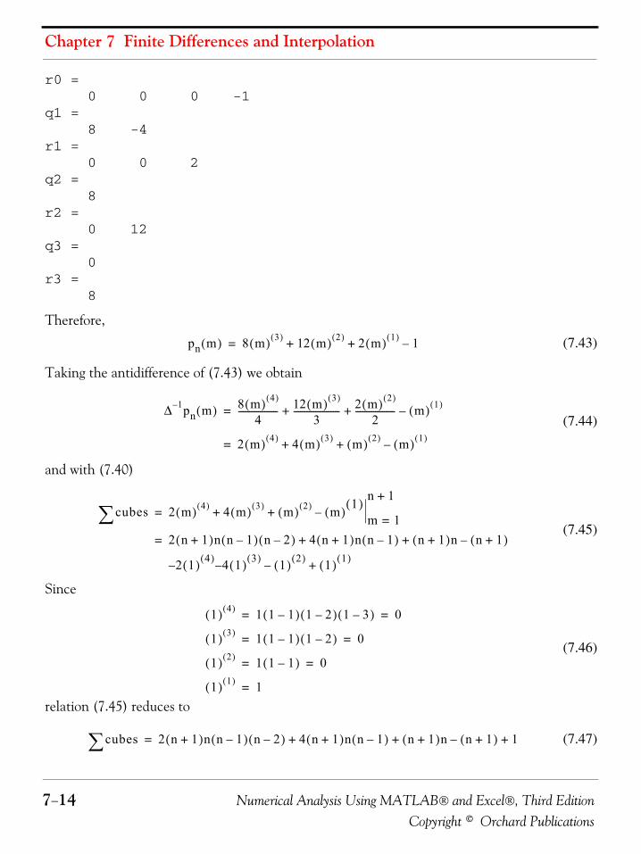
Chapter 7 Finite Differences and Interpolation
7−14 Numerical Analysis Using MATLAB® and Excel®, Third EditionCopyright © Orchard Publications
r0 = 0 0 0 -1q1 = 8 -4r1 = 0 0 2q2 = 8r2 = 0 12q3 = 0r3 = 8
Therefore,
(7.43)
Taking the antidifference of (7.43) we obtain
(7.44)
and with (7.40)
(7.45)
Since
(7.46)
relation (7.45) reduces to
(7.47)
pn m( ) 8 m( ) 3( ) 12 m( ) 2( ) 2 m( ) 1( ) 1–+ +=
Δ 1– pn m( ) 8 m( ) 4( )
4------------------ 12 m( ) 3( )
3--------------------- 2 m( ) 2( )
2------------------ m( ) 1( )–+ +=
2 m( ) 4( ) 4 m( ) 3( ) m( ) 2( ) m( ) 1( )–+ +=
cubes∑ 2 m( ) 4( ) 4 m( ) 3( ) m( ) 2( ) m( ) 1( )–+ + m 1=
n 1+=
2 n 1+( )n n 1–( ) n 2–( ) 4 n 1+( )n n 1–( ) n 1+( )n n 1+( )–+ +=
2 1( ) 4( )– 4– 1( ) 3( ) 1( ) 2( )
– 1( ) 1( )+
1( ) 4( ) 1 1 1–( ) 1 2–( ) 1 3–( ) 0= =
1( ) 3( ) 1 1 1–( ) 1 2–( ) 0= =
1( ) 2( ) 1 1 1–( ) 0= =
1( ) 1( ) 1=
cubes∑ 2 n 1+( )n n 1–( ) n 2–( ) 4 n 1+( )n n 1–( ) n 1+( )n n 1+( )– 1+ + +=
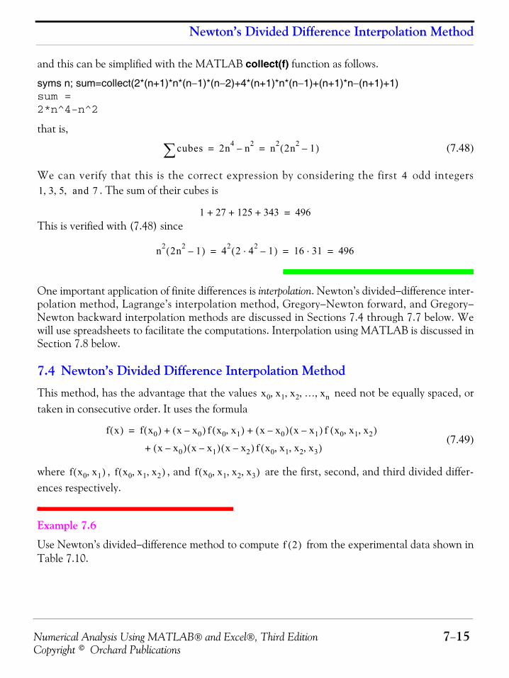
Numerical Analysis Using MATLAB® and Excel®, Third Edition 7−15Copyright © Orchard Publications
Newton’s Divided Difference Interpolation Method
and this can be simplified with the MATLAB collect(f) function as follows.
syms n; sum=collect(2*(n+1)*n*(n−1)*(n−2)+4*(n+1)*n*(n−1)+(n+1)*n−(n+1)+1)sum =2*n^4-n^2
that is,
(7.48)
We can verify that this is the correct expression by considering the first odd integers. The sum of their cubes is
This is verified with (7.48) since
One important application of finite differences is interpolation. Newton’s divided−difference inter-polation method, Lagrange’s interpolation method, Gregory−Newton forward, and Gregory−Newton backward interpolation methods are discussed in Sections 7.4 through 7.7 below. Wewill use spreadsheets to facilitate the computations. Interpolation using MATLAB is discussed inSection 7.8 below.
7.4 Newton’s Divided Difference Interpolation Method
This method, has the advantage that the values need not be equally spaced, ortaken in consecutive order. It uses the formula
(7.49)
where , , and are the first, second, and third divided differ-ences respectively.
Example 7.6
Use Newton’s divided−difference method to compute from the experimental data shown inTable 7.10.
cubes∑ 2n4 n2– n2 2n2 1–( )= =
41 3 5 and 7, , ,
1 27 125 343+ + + 496=
n2 2n2 1–( ) 42 2 42 1–⋅( ) 16 31⋅ 496= = =
x0 x1 x2 … xn, , , ,
f x( ) f x0( ) x x0–( ) f x0 x1,( ) x x0–( ) x x1–( ) f x0 x1 x2, ,( )+ +=
x x0–( ) x x1–( ) x x2–( ) f x0 x1 x2 x3, , ,( )+
f x0 x1,( ) f x0 x1 x2, ,( ) f x0 x1 x2 x3, , ,( )
f 2( )
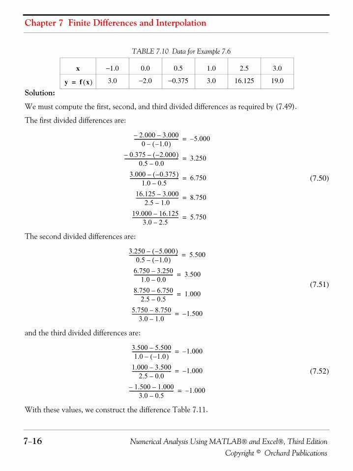
Chapter 7 Finite Differences and Interpolation
7−16 Numerical Analysis Using MATLAB® and Excel®, Third EditionCopyright © Orchard Publications
Solution:
We must compute the first, second, and third divided differences as required by (7.49).
The first divided differences are:
(7.50)
The second divided differences are:
(7.51)
and the third divided differences are:
(7.52)
With these values, we construct the difference Table 7.11.
TABLE 7.10 Data for Example 7.6
x −1.0 0.0 0.5 1.0 2.5 3.0
3.0 −2.0 −0.375 3.0 16.125 19.0y f x( )=
2.000– 3.000–0 1.0–( )–
------------------------------------- 5.000–=
0.375– 2.000–( )–0.5 0.0–
--------------------------------------------- 3.250=
3.000 0.375–( )–1.0 0.5–
----------------------------------------- 6.750=
16.125 3.000–2.5 1.0–
------------------------------------ 8.750=
19.000 16.125–3.0 2.5–
--------------------------------------- 5.750=
3.250 5.000–( )–0.5 1.0–( )–
----------------------------------------- 5.500=
6.750 3.250–1.0 0.0–
--------------------------------- 3.500=
8.750 6.750–2.5 0.5–
--------------------------------- 1.000=
5.750 8.750–3.0 1.0–
--------------------------------- 1.500–=
3.500 5.500–1.0 1.0–( )–
--------------------------------- 1.000–=
1.000 3.500–2.5 0.0–
--------------------------------- 1.000–=
1.500– 1.000–3.0 0.5–
------------------------------------- 1.000–=
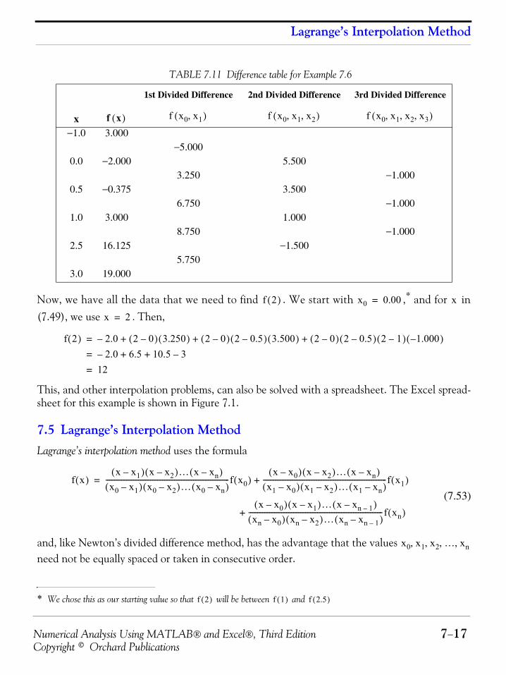
Numerical Analysis Using MATLAB® and Excel®, Third Edition 7−17Copyright © Orchard Publications
Lagrange’s Interpolation Method
Now, we have all the data that we need to find . We start with ,* and for in(7.49), we use . Then,
This, and other interpolation problems, can also be solved with a spreadsheet. The Excel spread-sheet for this example is shown in Figure 7.1.
7.5 Lagrange’s Interpolation MethodLagrange’s interpolation method uses the formula
(7.53)
and, like Newton’s divided difference method, has the advantage that the values need not be equally spaced or taken in consecutive order.
TABLE 7.11 Difference table for Example 7.6
1st Divided Difference 2nd Divided Difference 3rd Divided Difference
x−1.0 3.000
−5.0000.0 −2.000 5.500
3.250 −1.0000.5 −0.375 3.500
6.750 −1.0001.0 3.000 1.000
8.750 −1.0002.5 16.125 −1.500
5.7503.0 19.000
* We chose this as our starting value so that will be between and
f x( ) f x0 x1,( ) f x0 x1 x2, ,( ) f x0 x1 x2 x3, , ,( )
f 2( ) x0 0.00= x
f 2( ) f 1( ) f 2.5( )
x 2=
f 2( ) 2.0– 2 0–( ) 3.250( ) 2 0–( ) 2 0.5–( ) 3.500( ) 2 0–( ) 2 0.5–( ) 2 1–( ) 1.000–( )+ + +=
2.0– 6.5 10.5 3–+ +=
12=
f x( )x x1–( ) x x2–( )… x xn–( )
x0 x1–( ) x0 x2–( )… x0 xn–( )------------------------------------------------------------------------f x0( )
x x0–( ) x x2–( )… x xn–( )x1 x0–( ) x1 x2–( )… x1 xn–( )
------------------------------------------------------------------------f x1( )+=
x x0–( ) x x1–( )… x xn 1––( )
xn x0–( ) xn x2–( )… xn xn 1––( )------------------------------------------------------------------------------f xn( )+
x0 x1 x2 … xn, , , ,
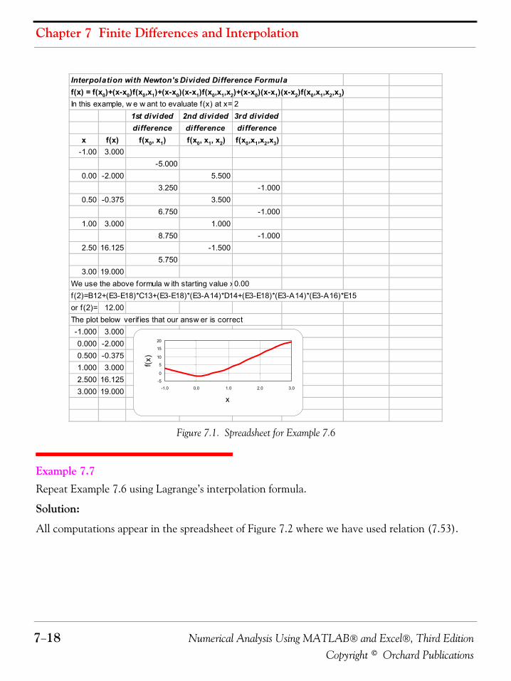
Chapter 7 Finite Differences and Interpolation
7−18 Numerical Analysis Using MATLAB® and Excel®, Third EditionCopyright © Orchard Publications
Figure 7.1. Spreadsheet for Example 7.6
Example 7.7 Repeat Example 7.6 using Lagrange’s interpolation formula.
Solution:
All computations appear in the spreadsheet of Figure 7.2 where we have used relation (7.53).
Interpolation with Newton's Divided Difference Formulaf(x) = f(x0)+(x-x0)f(x0,x1)+(x-x0)(x-x1)f(x0,x1,x2)+(x-x0)(x-x1)(x-x2)f(x0,x1,x2,x3)In this example, w e w ant to evaluate f(x) at x= 2
1st divided 2nd divided 3rd divideddifference difference difference
x f(x) f(x0, x1) f(x0, x1, x2) f(x0,x1,x2,x3)-1.00 3.000
-5.0000.00 -2.000 5.500
3.250 -1.0000.50 -0.375 3.500
6.750 -1.0001.00 3.000 1.000
8.750 -1.0002.50 16.125 -1.500
5.7503.00 19.000
We use the above formula w ith starting value x0.00f(2)=B12+(E3-E18)*C13+(E3-E18)*(E3-A14)*D14+(E3-E18)*(E3-A14)*(E3-A16)*E15or f(2)= 12.00The plot below verif ies that our answ er is correct-1.000 3.0000.000 -2.0000.500 -0.3751.000 3.0002.500 16.1253.000 19.000
-5
0
5
10
15
20
-1.0 0.0 1.0 2.0 3.0
x
f(x)
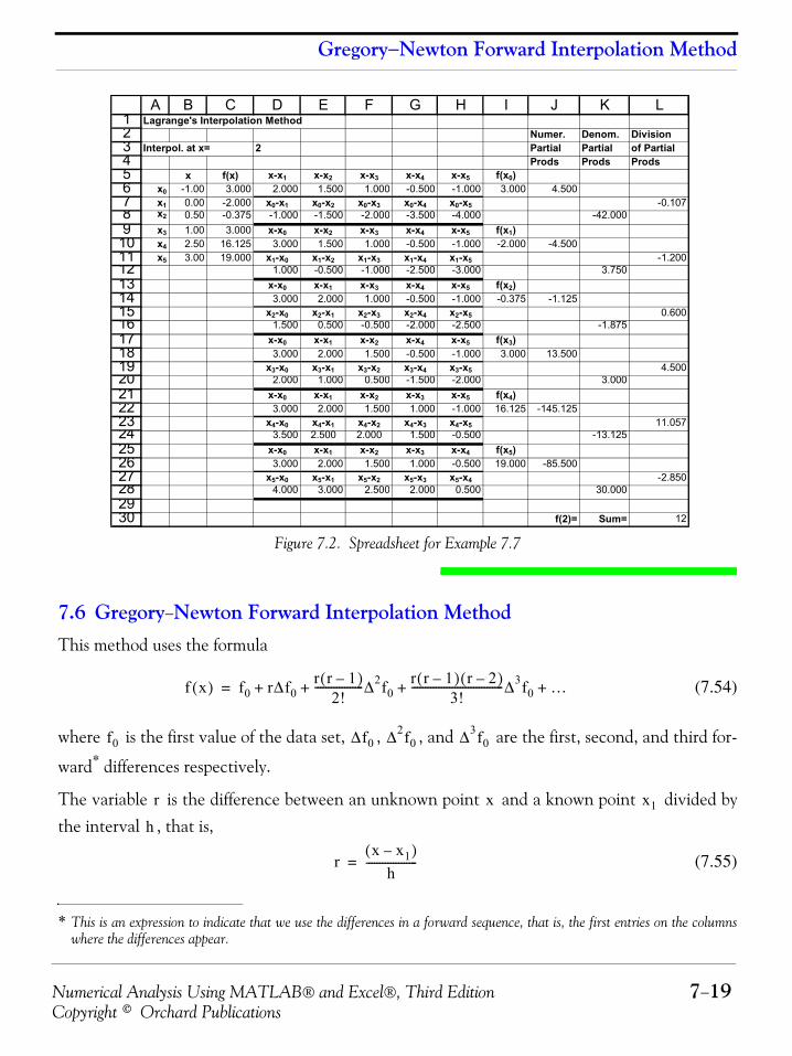
Numerical Analysis Using MATLAB® and Excel®, Third Edition 7−19Copyright © Orchard Publications
Gregory−Newton Forward Interpolation Method
Figure 7.2. Spreadsheet for Example 7.7
7.6 Gregory−Newton Forward Interpolation MethodThis method uses the formula
(7.54)
where is the first value of the data set, , , and are the first, second, and third for-
ward* differences respectively.
The variable is the difference between an unknown point and a known point divided bythe interval , that is,
(7.55)
* This is an expression to indicate that we use the differences in a forward sequence, that is, the first entries on the columnswhere the differences appear.
123456789
101112131415161718192021222324252627282930
A B C D E F G H I J K LLagrange's Interpolation Method
Numer. Denom. DivisionInterpol. at x= 2 Partial Partial of Partial
Prods Prods Prodsx f(x) x-x1 x-x2 x-x3 x-x4 x-x5 f(x0)
x0 -1.00 3.000 2.000 1.500 1.000 -0.500 -1.000 3.000 4.500x1 0.00 -2.000 x0-x1 x0-x2 x0-x3 x0-x4 x0-x5 -0.107x2 0.50 -0.375 -1.000 -1.500 -2.000 -3.500 -4.000 -42.000x3 1.00 3.000 x-x0 x-x2 x-x3 x-x4 x-x5 f(x1)x4 2.50 16.125 3.000 1.500 1.000 -0.500 -1.000 -2.000 -4.500x5 3.00 19.000 x1-x0 x1-x2 x1-x3 x1-x4 x1-x5 -1.200
1.000 -0.500 -1.000 -2.500 -3.000 3.750x-x0 x-x1 x-x3 x-x4 x-x5 f(x2)3.000 2.000 1.000 -0.500 -1.000 -0.375 -1.125
x2-x0 x2-x1 x2-x3 x2-x4 x2-x5 0.6001.500 0.500 -0.500 -2.000 -2.500 -1.875
x-x0 x-x1 x-x2 x-x4 x-x5 f(x3)3.000 2.000 1.500 -0.500 -1.000 3.000 13.500
x3-x0 x3-x1 x3-x2 x3-x4 x3-x5 4.5002.000 1.000 0.500 -1.500 -2.000 3.000
x-x0 x-x1 x-x2 x-x3 x-x5 f(x4)3.000 2.000 1.500 1.000 -1.000 16.125 -145.125
x4-x0 x4-x1 x4-x2 x4-x3 x4-x5 11.0573.500 2.500 2.000 1.500 -0.500 -13.125
x-x0 x-x1 x-x2 x-x3 x-x4 f(x5)3.000 2.000 1.500 1.000 -0.500 19.000 -85.500
x5-x0 x5-x1 x5-x2 x5-x3 x5-x4 -2.8504.000 3.000 2.500 2.000 0.500 30.000
f(2)= Sum= 12
f x( ) f0 rΔf0r r 1–( )
2!------------------Δ2f0
r r 1–( ) r 2–( )3!
----------------------------------Δ3f0 …+ + + +=
f0 Δf0 Δ2f0 Δ3f0
r x x1
h
rx x1–( )
h-------------------=
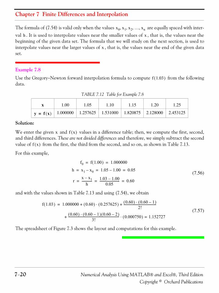
Chapter 7 Finite Differences and Interpolation
7−20 Numerical Analysis Using MATLAB® and Excel®, Third EditionCopyright © Orchard Publications
The formula of (7.54) is valid only when the values are equally spaced with inter-val . It is used to interpolate values near the smaller values of , that is, the values near thebeginning of the given data set. The formula that we will study on the next section, is used tointerpolate values near the larger values of , that is, the values near the end of the given dataset.
Example 7.8
Use the Gregory−Newton forward interpolation formula to compute from the followingdata.
Solution:
We enter the given and values in a difference table; then, we compute the first, second,and third differences. These are not divided differences and therefore, we simply subtract the secondvalue of from the first, the third from the second, and so on, as shown in Table 7.13.
For this example,
(7.56)
and with the values shown in Table 7.13 and using (7.54), we obtain
(7.57)
The spreadsheet of Figure 7.3 shows the layout and computations for this example.
TABLE 7.12 Table for Example 7.8
x 1.00 1.05 1.10 1.15 1.20 1.25
1.000000 1.257625 1.531000 1.820875 2.128000 2.453125
x0 x1 x2 … xn, , , ,
h x
x
f 1.03( )
y f x( )=
x f x( )
f x( )
f0 f 1.00( ) 1.000000= =
h x1 x0– 1.05 1.00– 0.05= = =
rx x1–
h-------------- 1.03 1.00–
0.05--------------------------- 0.60= = =
f 1.03( ) 1.000000 0.60( ) 0.257625( )⋅ 0.60( ) 0.60 1–( )⋅2!
--------------------------------------------+ +=
0.60( ) 0.60 1–( ) 0.60 2–( )⋅3!
-------------------------------------------------------------------- 0.000750( )⋅ 1.152727=+
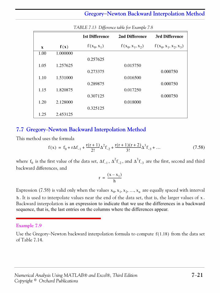
Numerical Analysis Using MATLAB® and Excel®, Third Edition 7−21Copyright © Orchard Publications
Gregory−Newton Backward Interpolation Method
7.7 Gregory−Newton Backward Interpolation MethodThis method uses the formula
(7.58)
where is the first value of the data set, , , and are the first, second and thirdbackward differences, and
Expression (7.58) is valid only when the values are equally spaced with interval. It is used to interpolate values near the end of the data set, that is, the larger values of .
Backward interpolation is an expression to indicate that we use the differences in a backwardsequence, that is, the last entries on the columns where the differences appear.
Example 7.9
Use the Gregory−Newton backward interpolation formula to compute from the data setof Table 7.14.
TABLE 7.13 Difference table for Example 7.8
1st Difference 2nd Difference 3rd Difference
x1.00 1.000000
0.2576251.05 1.257625 0.015750
0.273375 0.0007501.10 1.531000 0.016500
0.289875 0.0007501.15 1.820875 0.017250
0.307125 0.0007501.20 2.128000 0.018000
0.3251251.25 2.453125
f x( ) f x0 x1,( ) f x0 x1 x2, ,( ) f x0 x1 x2 x3, , ,( )
f x( ) f0 rΔf 1–r r 1+( )
2!------------------Δ2f 2–
r r 1+( ) r 2+( )3!
-----------------------------------Δ3f 3– …+ + + +=
f0 Δf 1– Δ2f 2– Δ3f 3–
rx x1–( )
h-------------------=
x0 x1 x2 … xn, , , ,
h x
f 1.18( )
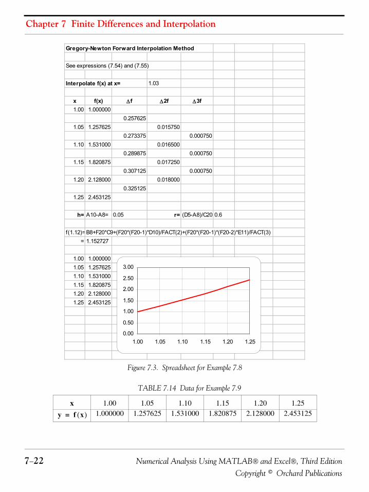
Chapter 7 Finite Differences and Interpolation
7−22 Numerical Analysis Using MATLAB® and Excel®, Third EditionCopyright © Orchard Publications
Figure 7.3. Spreadsheet for Example 7.8
TABLE 7.14 Data for Example 7.9
x 1.00 1.05 1.10 1.15 1.20 1.251.000000 1.257625 1.531000 1.820875 2.128000 2.453125
Gregory-Newton Forward Interpolation Method
See expressions (7.54) and (7.55)
Interpolate f(x) at x= 1.03
x f(x) Δf Δ2f Δ3f1.00 1.000000
0.2576251.05 1.257625 0.015750
0.273375 0.0007501.10 1.531000 0.016500
0.289875 0.0007501.15 1.820875 0.017250
0.307125 0.0007501.20 2.128000 0.018000
0.3251251.25 2.453125
h= A10-A8= 0.05 r= (D5-A8)/C20=0.6
f(1.12)=B8+F20*C9+(F20*(F20-1)*D10)/FACT(2)+(F20*(F20-1)*(F20-2)*E11)/FACT(3)= 1.152727
1.00 1.0000001.05 1.2576251.10 1.5310001.15 1.8208751.20 2.1280001.25 2.453125
0.00
0.50
1.00
1.50
2.00
2.50
3.00
1.00 1.05 1.10 1.15 1.20 1.25
y f x( )=
Numerical Analysis Using MATLAB® and Excel®, Third Edition 7−23Copyright © Orchard Publications
Gregory−Newton Backward Interpolation Method
Solution:
We arbitrarily choose as our starting point since lies between and. Then,
and
Now, by (7.58) we have:
The computations were made with the spreadsheet of Figure 7.4.
If the increments in values are small, we can use the Excel VLOOKUP function to performinterpolation. The syntax of this function is as follows.
VLOOKUP(lookup_value, table_array, col_index_num, range lookup)
where:
lookup_value is the value being searched in the first column of the lookup table
table_array are the columns forming a rectangular range or array
col_index_num is the column where the answer will be found
range lookup is a logical value (TRUE or FALSE) that specifies whether we require VLOOKUP tofind an exact or an approximate match. If TRUE is omitted, an approximate match is returned.In other words, if an exact match is not found, the next largest value that is less than thelookup_value is returned. If FALSE is specified, VLOOKUP will attempt to find an exact match,and if one is not found, the error value #N/A will be returned.
A sample spreadsheet is shown in Figure 7.5 where the values of x extend from −5 to +5 volts.Only a partial table is shown.
f0 2.128000= f 1.18( ) f 1.15( )
f 1.20( )h 1.20 1.15– 0.05= =
r x x1–( ) h⁄ 1.18 1.20–( ) 0.05⁄ 0.4–= = =
f 1.18( ) 2.128 0.4–( ) 0.307125( ) 0.4–( ) 0.4– 1+( )2!
------------------------------------------ 0.01725( )
0.4–( ) 0.4– 1+( ) 0.4– 2+( )3!
-------------------------------------------------------------------- 0.00075( ) 2.003032=
+ +
+
=
x
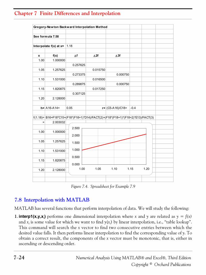
Chapter 7 Finite Differences and Interpolation
7−24 Numerical Analysis Using MATLAB® and Excel®, Third EditionCopyright © Orchard Publications
Figure 7.4. Spreadsheet for Example 7.9
7.8 Interpolation with MATLABMATLAB has several functions that perform interpolation of data. We will study the following:
1. interp1(x,y,xi) performs one dimensional interpolation where x and y are related as y = f(x)and xi is some value for which we want to find y(xi) by linear interpolation, i.e., “table lookup”.This command will search the x vector to find two consecutive entries between which thedesired value falls. It then performs linear interpolation to find the corresponding value of y. Toobtain a correct result, the components of the x vector must be monotonic, that is, either inascending or descending order.
Gregory-Newton Backward Interpolation Method
See formula 7.58
Interpolate f(x) at x= 1.18
x f(x) Δ f Δ2f Δ3f1.00 1.000000
0.2576251.05 1.257625 0.015750
0.273375 0.0007501.10 1.531000 0.016500
0.289875 0.0007501.15 1.820875 0.017250
0.3071251.20 2.128000
h= A16-A14= 0.05 r= (C5-A16)/C18= -0.4
f(1.18)= B16+F18*C15+(F18*(F18+1)*D14)/FACT(2)+(F18*(F18+1)*(F18+2)*E13)/FACT(3)= 2.003032
1.00 1.000000
1.05 1.257625
1.10 1.531000
1.15 1.820875
1.20 2.128000
0.000
0.500
1.000
1.500
2.000
2.500
1.00 1.05 1.10 1.15 1.20
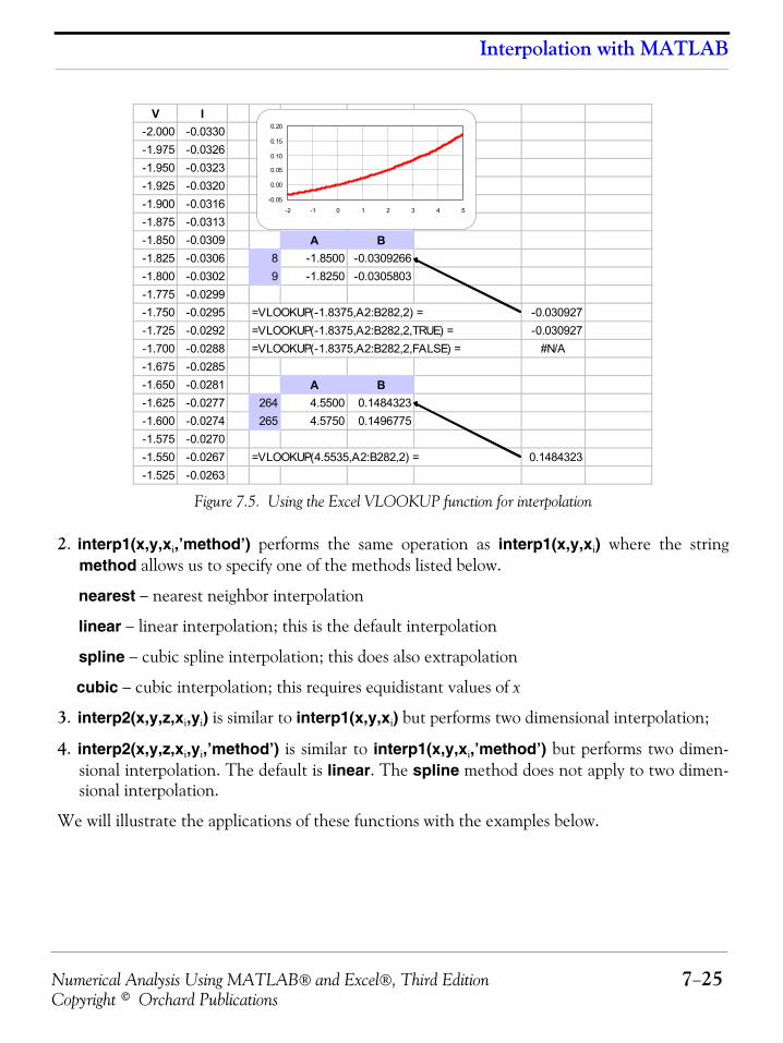
Numerical Analysis Using MATLAB® and Excel®, Third Edition 7−25Copyright © Orchard Publications
Interpolation with MATLAB
Figure 7.5. Using the Excel VLOOKUP function for interpolation
2. interp1(x,y,xi,’method’) performs the same operation as interp1(x,y,xi) where the stringmethod allows us to specify one of the methods listed below.
nearest − nearest neighbor interpolation
linear − linear interpolation; this is the default interpolation
spline − cubic spline interpolation; this does also extrapolation
cubic − cubic interpolation; this requires equidistant values of x
3. interp2(x,y,z,xi,yi) is similar to interp1(x,y,xi) but performs two dimensional interpolation;
4. interp2(x,y,z,xi,yi,’method’) is similar to interp1(x,y,xi,’method’) but performs two dimen-sional interpolation. The default is linear. The spline method does not apply to two dimen-sional interpolation.
We will illustrate the applications of these functions with the examples below.
V I-2.000 -0.0330-1.975 -0.0326-1.950 -0.0323-1.925 -0.0320-1.900 -0.0316-1.875 -0.0313-1.850 -0.0309 A B-1.825 -0.0306 8 -1.8500 -0.0309266-1.800 -0.0302 9 -1.8250 -0.0305803-1.775 -0.0299-1.750 -0.0295 =VLOOKUP(-1.8375,A2:B282,2) = -0.030927-1.725 -0.0292 =VLOOKUP(-1.8375,A2:B282,2,TRUE) = -0.030927-1.700 -0.0288 =VLOOKUP(-1.8375,A2:B282,2,FALSE) = #N/A-1.675 -0.0285-1.650 -0.0281 A B-1.625 -0.0277 264 4.5500 0.1484323-1.600 -0.0274 265 4.5750 0.1496775-1.575 -0.0270-1.550 -0.0267 =VLOOKUP(4.5535,A2:B282,2) = 0.1484323-1.525 -0.0263
-0.05
0.00
0.05
0.10
0.15
0.20
-2 -1 0 1 2 3 4 5
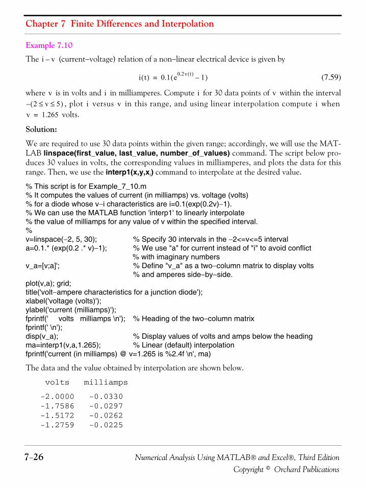
Chapter 7 Finite Differences and Interpolation
7−26 Numerical Analysis Using MATLAB® and Excel®, Third EditionCopyright © Orchard Publications
Example 7.10
The (current−voltage) relation of a non−linear electrical device is given by
(7.59)
where is in volts and in milliamperes. Compute for 30 data points of within the interval, plot versus in this range, and using linear interpolation compute when
volts.
Solution:
We are required to use 30 data points within the given range; accordingly, we will use the MAT-LAB linspace(first_value, last_value, number_of_values) command. The script below pro-duces 30 values in volts, the corresponding values in milliamperes, and plots the data for thisrange. Then, we use the interp1(x,y,xi) command to interpolate at the desired value.
% This script is for Example_7_10.m% It computes the values of current (in milliamps) vs. voltage (volts)% for a diode whose v−i characteristics are i=0.1(exp(0.2v)−1).% We can use the MATLAB function 'interp1' to linearly interpolate% the value of milliamps for any value of v within the specified interval.%v=linspace(−2, 5, 30); % Specify 30 intervals in the −2<=v<=5 intervala=0.1.* (exp(0.2 .* v)−1); % We use "a" for current instead of "i" to avoid conflict
% with imaginary numbersv_a=[v;a]'; % Define "v_a" as a two−column matrix to display volts
% and amperes side−by−side.plot(v,a); grid;title('volt−ampere characteristics for a junction diode');xlabel('voltage (volts)');ylabel('current (milliamps)');fprintf(' volts milliamps \n'); % Heading of the two−column matrixfprintf(' \n');disp(v_a); % Display values of volts and amps below the headingma=interp1(v,a,1.265); % Linear (default) interpolationfprintf('current (in milliamps) @ v=1.265 is %2.4f \n', ma)
The data and the value obtained by interpolation are shown below.
volts milliamps
-2.0000 -0.0330 -1.7586 -0.0297 -1.5172 -0.0262 -1.2759 -0.0225
i v–
i t( ) 0.1 e0.2v t( ) 1–( )=
v i i v2 v 5≤ ≤( )– i v i
v 1.265=
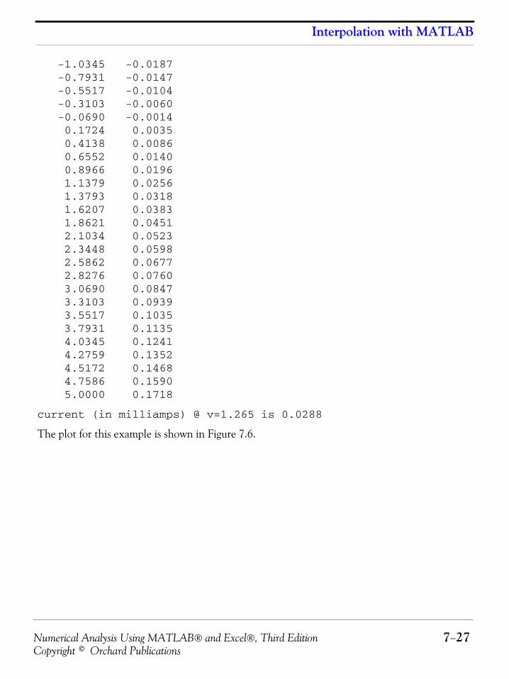
Numerical Analysis Using MATLAB® and Excel®, Third Edition 7−27Copyright © Orchard Publications
Interpolation with MATLAB
-1.0345 -0.0187 -0.7931 -0.0147 -0.5517 -0.0104 -0.3103 -0.0060 -0.0690 -0.0014 0.1724 0.0035 0.4138 0.0086 0.6552 0.0140 0.8966 0.0196 1.1379 0.0256 1.3793 0.0318 1.6207 0.0383 1.8621 0.0451 2.1034 0.0523 2.3448 0.0598 2.5862 0.0677 2.8276 0.0760 3.0690 0.0847 3.3103 0.0939 3.5517 0.1035 3.7931 0.1135 4.0345 0.1241 4.2759 0.1352 4.5172 0.1468 4.7586 0.1590 5.0000 0.1718
current (in milliamps) @ v=1.265 is 0.0288
The plot for this example is shown in Figure 7.6.
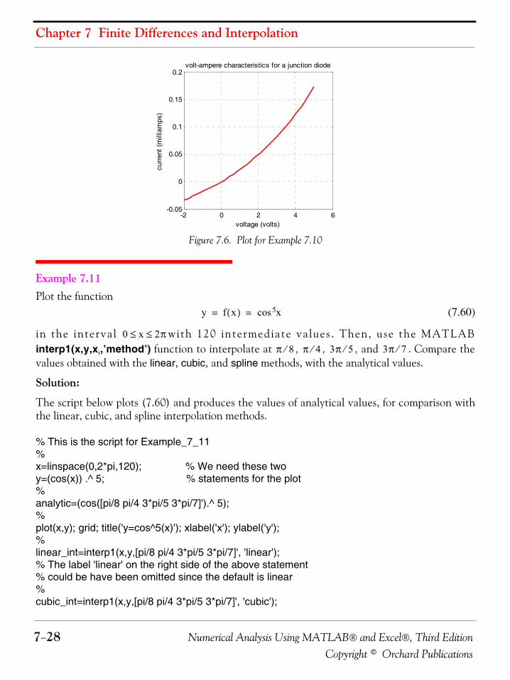
Chapter 7 Finite Differences and Interpolation
7−28 Numerical Analysis Using MATLAB® and Excel®, Third EditionCopyright © Orchard Publications
Figure 7.6. Plot for Example 7.10
Example 7.11 Plot the function
(7.60)
in the interval with 120 intermediate values . Then, use the MATLABinterp1(x,y,xi,’method’) function to interpolate at , , , and . Compare thevalues obtained with the linear, cubic, and spline methods, with the analytical values.
Solution:
The script below plots (7.60) and produces the values of analytical values, for comparison withthe linear, cubic, and spline interpolation methods.
% This is the script for Example_7_11%x=linspace(0,2*pi,120); % We need these twoy=(cos(x)) .^ 5; % statements for the plot%analytic=(cos([pi/8 pi/4 3*pi/5 3*pi/7]').^ 5);% plot(x,y); grid; title('y=cos^5(x)'); xlabel('x'); ylabel('y');%linear_int=interp1(x,y,[pi/8 pi/4 3*pi/5 3*pi/7]', 'linear');% The label 'linear' on the right side of the above statement% could be have been omitted since the default is linear%cubic_int=interp1(x,y,[pi/8 pi/4 3*pi/5 3*pi/7]', 'cubic');
-2 0 2 4 6-0.05
0
0.05
0.1
0.15
0.2volt-ampere characteristics for a junction diode
voltage (volts)
curr
ent (
mill
iam
ps)
y f x( ) x5cos= =
0 x 2π≤ ≤π 8⁄ π 4⁄ 3π 5⁄ 3π 7⁄
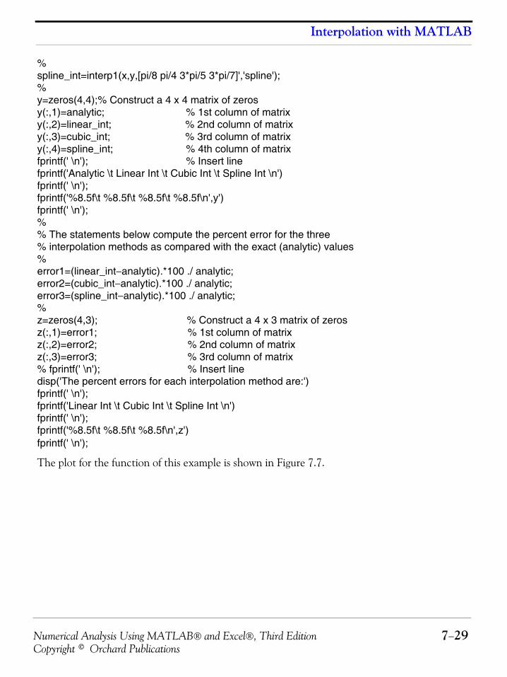
Numerical Analysis Using MATLAB® and Excel®, Third Edition 7−29Copyright © Orchard Publications
Interpolation with MATLAB
%spline_int=interp1(x,y,[pi/8 pi/4 3*pi/5 3*pi/7]','spline');% y=zeros(4,4);% Construct a 4 x 4 matrix of zerosy(:,1)=analytic; % 1st column of matrixy(:,2)=linear_int; % 2nd column of matrixy(:,3)=cubic_int; % 3rd column of matrixy(:,4)=spline_int; % 4th column of matrixfprintf(' \n'); % Insert linefprintf('Analytic \t Linear Int \t Cubic Int \t Spline Int \n')fprintf(' \n');fprintf('%8.5f\t %8.5f\t %8.5f\t %8.5f\n',y')fprintf(' \n');% % The statements below compute the percent error for the three% interpolation methods as compared with the exact (analytic) values%error1=(linear_int−analytic).*100 ./ analytic;error2=(cubic_int−analytic).*100 ./ analytic;error3=(spline_int−analytic).*100 ./ analytic;%z=zeros(4,3); % Construct a 4 x 3 matrix of zerosz(:,1)=error1; % 1st column of matrixz(:,2)=error2; % 2nd column of matrixz(:,3)=error3; % 3rd column of matrix% fprintf(' \n'); % Insert linedisp('The percent errors for each interpolation method are:')fprintf(' \n');fprintf('Linear Int \t Cubic Int \t Spline Int \n')fprintf(' \n');fprintf('%8.5f\t %8.5f\t %8.5f\n',z')fprintf(' \n');
The plot for the function of this example is shown in Figure 7.7.
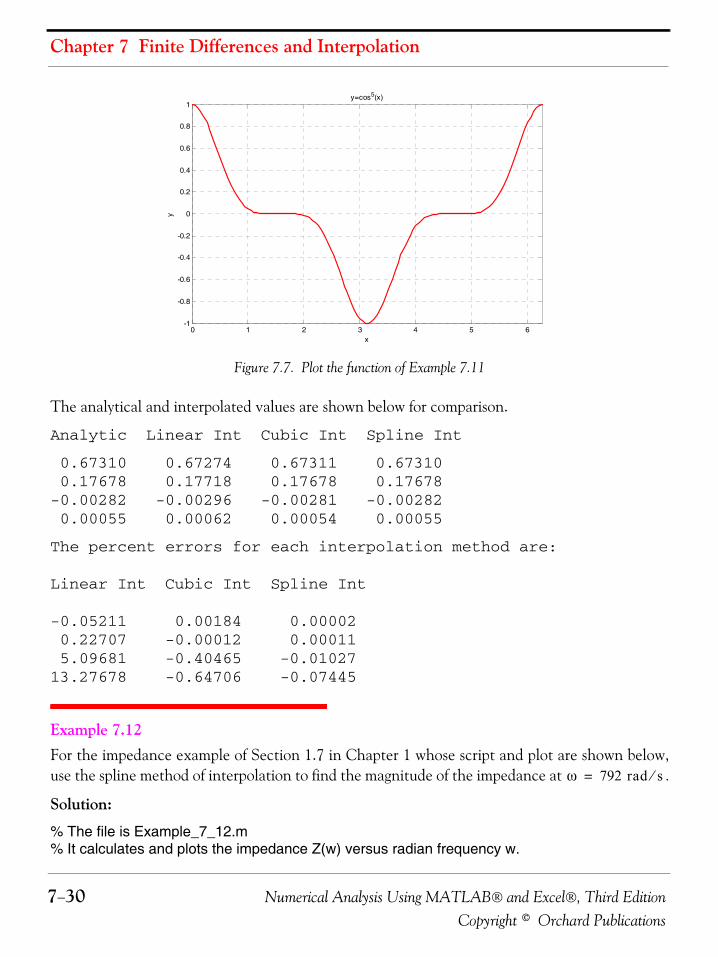
Chapter 7 Finite Differences and Interpolation
7−30 Numerical Analysis Using MATLAB® and Excel®, Third EditionCopyright © Orchard Publications
Figure 7.7. Plot the function of Example 7.11
The analytical and interpolated values are shown below for comparison.
Analytic Linear Int Cubic Int Spline Int
0.67310 0.67274 0.67311 0.67310 0.17678 0.17718 0.17678 0.17678-0.00282 -0.00296 -0.00281 -0.00282 0.00055 0.00062 0.00054 0.00055
The percent errors for each interpolation method are: Linear Int Cubic Int Spline Int -0.05211 0.00184 0.00002 0.22707 -0.00012 0.00011 5.09681 -0.40465 -0.0102713.27678 -0.64706 -0.07445
Example 7.12 For the impedance example of Section 1.7 in Chapter 1 whose script and plot are shown below,use the spline method of interpolation to find the magnitude of the impedance at .
Solution:
% The file is Example_7_12.m% It calculates and plots the impedance Z(w) versus radian frequency w.
0 1 2 3 4 5 6-1
-0.8
-0.6
-0.4
-0.2
0
0.2
0.4
0.6
0.8
1y=cos5(x)
x
y
ω 792 rad s⁄=
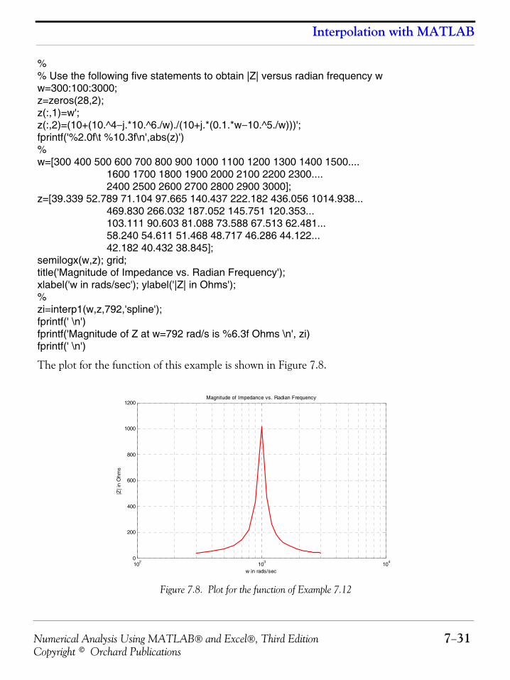
Numerical Analysis Using MATLAB® and Excel®, Third Edition 7−31Copyright © Orchard Publications
Interpolation with MATLAB
%% Use the following five statements to obtain |Z| versus radian frequency ww=300:100:3000;z=zeros(28,2);z(:,1)=w';z(:,2)=(10+(10.^4−j.*10.^6./w)./(10+j.*(0.1.*w−10.^5./w)))';fprintf('%2.0f\t %10.3f\n',abs(z)')%w=[300 400 500 600 700 800 900 1000 1100 1200 1300 1400 1500.... 1600 1700 1800 1900 2000 2100 2200 2300.... 2400 2500 2600 2700 2800 2900 3000];z=[39.339 52.789 71.104 97.665 140.437 222.182 436.056 1014.938... 469.830 266.032 187.052 145.751 120.353... 103.111 90.603 81.088 73.588 67.513 62.481... 58.240 54.611 51.468 48.717 46.286 44.122... 42.182 40.432 38.845];semilogx(w,z); grid;title('Magnitude of Impedance vs. Radian Frequency');xlabel('w in rads/sec'); ylabel('|Z| in Ohms');%zi=interp1(w,z,792,'spline');fprintf(' \n')fprintf('Magnitude of Z at w=792 rad/s is %6.3f Ohms \n', zi)fprintf(' \n')
The plot for the function of this example is shown in Figure 7.8.
Figure 7.8. Plot for the function of Example 7.12
102 103 1040
200
400
600
800
1000
1200Magnitude of Impedance vs. Radian Frequency
w in rads/sec
|Z| i
n O
hms
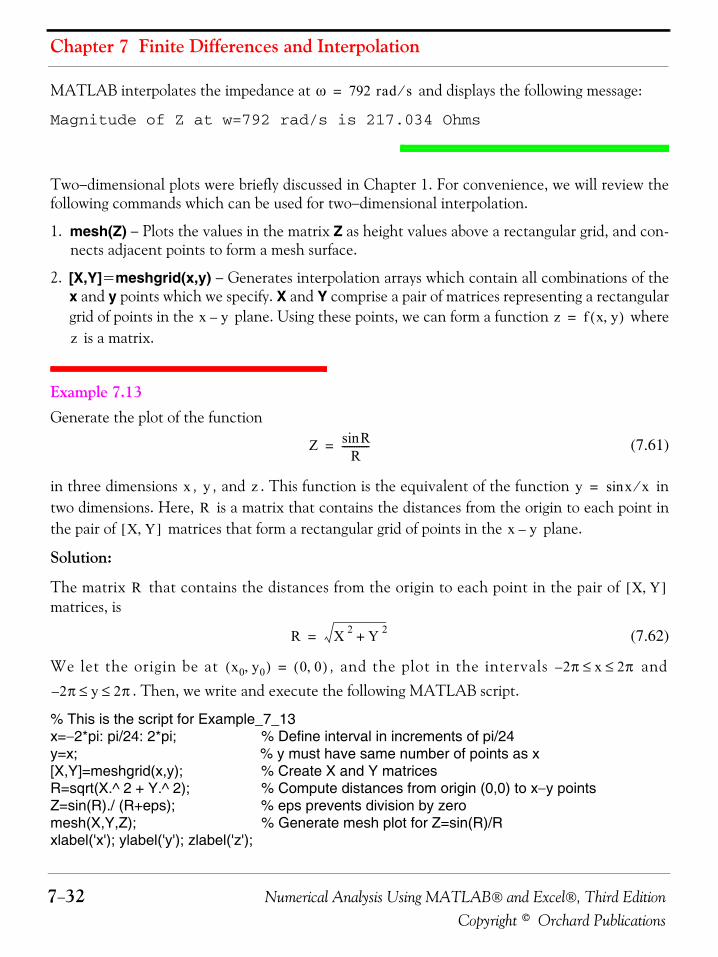
Chapter 7 Finite Differences and Interpolation
7−32 Numerical Analysis Using MATLAB® and Excel®, Third EditionCopyright © Orchard Publications
MATLAB interpolates the impedance at and displays the following message:
Magnitude of Z at w=792 rad/s is 217.034 Ohms
Two−dimensional plots were briefly discussed in Chapter 1. For convenience, we will review thefollowing commands which can be used for two−dimensional interpolation.
1. mesh(Z) − Plots the values in the matrix Z as height values above a rectangular grid, and con-nects adjacent points to form a mesh surface.
2. [X,Y]=meshgrid(x,y) − Generates interpolation arrays which contain all combinations of thex and y points which we specify. X and Y comprise a pair of matrices representing a rectangulargrid of points in the plane. Using these points, we can form a function where
is a matrix.
Example 7.13 Generate the plot of the function
(7.61)
in three dimensions , , and . This function is the equivalent of the function intwo dimensions. Here, is a matrix that contains the distances from the origin to each point inthe pair of matrices that form a rectangular grid of points in the plane.
Solution:
The matrix that contains the distances from the origin to each point in the pair of matrices, is
(7.62)
We let the origin be at , and the plot in the intervals and. Then, we write and execute the following MATLAB script.
% This is the script for Example_7_13x=−2*pi: pi/24: 2*pi; % Define interval in increments of pi/24y=x; % y must have same number of points as x[X,Y]=meshgrid(x,y); % Create X and Y matricesR=sqrt(X.^ 2 + Y.^ 2); % Compute distances from origin (0,0) to x−y pointsZ=sin(R)./ (R+eps); % eps prevents division by zeromesh(X,Y,Z); % Generate mesh plot for Z=sin(R)/Rxlabel('x'); ylabel('y'); zlabel('z');
ω 792 rad s⁄=
x y– z f x y,( )=
z
Z RsinR
-----------=
x y z y xsin x⁄=
RX Y,[ ] x y–
R X Y,[ ]
R X 2 Y 2+=
x0 y0,( ) 0 0,( )= 2π– x 2π≤ ≤
2π– y 2π≤ ≤
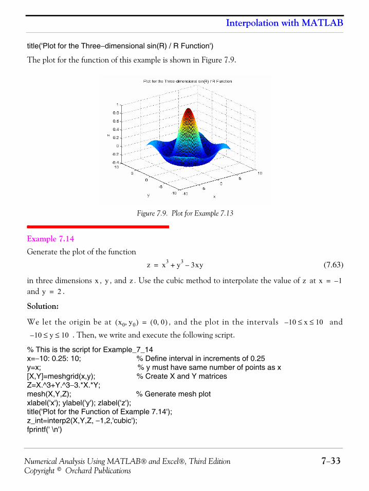
Numerical Analysis Using MATLAB® and Excel®, Third Edition 7−33Copyright © Orchard Publications
Interpolation with MATLAB
title('Plot for the Three−dimensional sin(R) / R Function')
The plot for the function of this example is shown in Figure 7.9.
Figure 7.9. Plot for Example 7.13
Example 7.14 Generate the plot of the function
(7.63)
in three dimensions , , and . Use the cubic method to interpolate the value of at and .
Solution:
We let the origin be at , and the plot in the intervals and
. Then, we write and execute the following script.
% This is the script for Example_7_14x=−10: 0.25: 10; % Define interval in increments of 0.25y=x; % y must have same number of points as x[X,Y]=meshgrid(x,y); % Create X and Y matricesZ=X.^3+Y.^3−3.*X.*Y;mesh(X,Y,Z); % Generate mesh plotxlabel('x'); ylabel('y'); zlabel('z');title('Plot for the Function of Example 7.14');z_int=interp2(X,Y,Z, −1,2,'cubic');fprintf(' \n')
z x3 y3 3xy–+=
x y z z x 1–=
y 2=
x0 y0,( ) 0 0,( )= 10– x 10≤ ≤
10– y 10≤ ≤
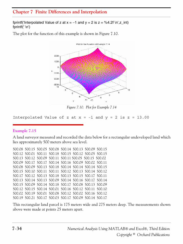
Chapter 7 Finite Differences and Interpolation
7−34 Numerical Analysis Using MATLAB® and Excel®, Third EditionCopyright © Orchard Publications
fprintf('Interpolated Value of z at x = −1 and y = 2 is z = %4.2f \n',z_int)fprintf(' \n')
The plot for the function of this example is shown in Figure 7.10.
Figure 7.10. Plot for Example 7.14
Interpolated Value of z at x = -1 and y = 2 is z = 13.00
Example 7.15 A land surveyor measured and recorded the data below for a rectangular undeveloped land whichlies approximately 500 meters above sea level.
500.08 500.15 500.05 500.08 500.14 500.13 500.09 500.15500.12 500.01 500.11 500.18 500.15 500.12 500.05 500.15500.13 500.12 500.09 500.11 500.11 500.05 500.15 500.02500.09 500.17 500.17 500.14 500.16 500.09 500.02 500.11500.08 500.09 500.13 500.18 500.14 500.14 500.14 500.15500.15 500.10 500.11 500.11 500.12 500.13 500.14 500.12500.17 500.12 500.13 500.18 500.13 500.15 500.17 500.11500.13 500.14 500.13 500.09 500.14 500.16 500.17 500.14500.15 500.09 500.14 500.18 500.17 500.08 500.13 500.09500.12 500.15 500.14 500.01 500.16 500.12 500.11 500.10500.02 500.19 500.01 500.08 500.12 500.02 500.16 500.12500.19 500.21 500.17 500.03 500.17 500.09 500.14 500.17
This rectangular land parcel is 175 meters wide and 275 meters deep. The measurements shownabove were made at points 25 meters apart.
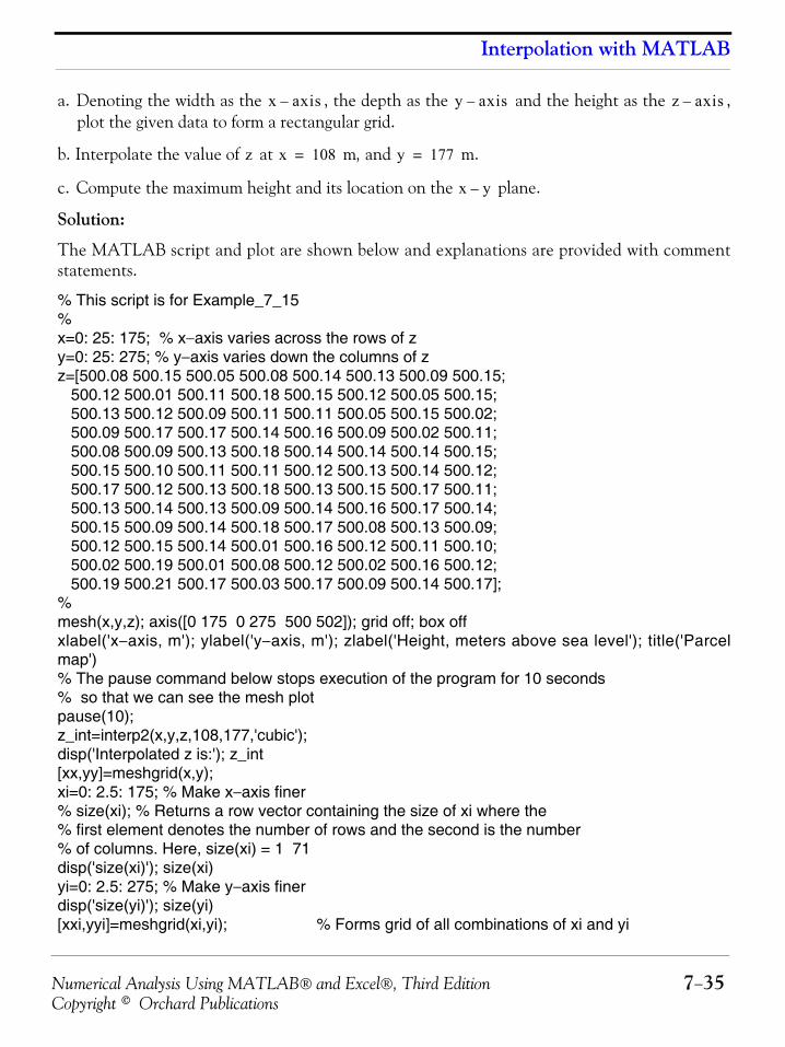
Numerical Analysis Using MATLAB® and Excel®, Third Edition 7−35Copyright © Orchard Publications
Interpolation with MATLAB
a. Denoting the width as the , the depth as the and the height as the ,plot the given data to form a rectangular grid.
b. Interpolate the value of at m, and m.
c. Compute the maximum height and its location on the plane.
Solution:
The MATLAB script and plot are shown below and explanations are provided with commentstatements.
% This script is for Example_7_15%x=0: 25: 175; % x−axis varies across the rows of zy=0: 25: 275; % y−axis varies down the columns of zz=[500.08 500.15 500.05 500.08 500.14 500.13 500.09 500.15; 500.12 500.01 500.11 500.18 500.15 500.12 500.05 500.15; 500.13 500.12 500.09 500.11 500.11 500.05 500.15 500.02; 500.09 500.17 500.17 500.14 500.16 500.09 500.02 500.11; 500.08 500.09 500.13 500.18 500.14 500.14 500.14 500.15; 500.15 500.10 500.11 500.11 500.12 500.13 500.14 500.12; 500.17 500.12 500.13 500.18 500.13 500.15 500.17 500.11; 500.13 500.14 500.13 500.09 500.14 500.16 500.17 500.14; 500.15 500.09 500.14 500.18 500.17 500.08 500.13 500.09; 500.12 500.15 500.14 500.01 500.16 500.12 500.11 500.10; 500.02 500.19 500.01 500.08 500.12 500.02 500.16 500.12; 500.19 500.21 500.17 500.03 500.17 500.09 500.14 500.17];%mesh(x,y,z); axis([0 175 0 275 500 502]); grid off; box offxlabel('x−axis, m'); ylabel('y−axis, m'); zlabel('Height, meters above sea level'); title('Parcelmap')% The pause command below stops execution of the program for 10 seconds% so that we can see the mesh plotpause(10);z_int=interp2(x,y,z,108,177,'cubic');disp('Interpolated z is:'); z_int[xx,yy]=meshgrid(x,y);xi=0: 2.5: 175; % Make x−axis finer% size(xi); % Returns a row vector containing the size of xi where the% first element denotes the number of rows and the second is the number% of columns. Here, size(xi) = 1 71disp('size(xi)'); size(xi)yi=0: 2.5: 275; % Make y−axis finerdisp('size(yi)'); size(yi)[xxi,yyi]=meshgrid(xi,yi); % Forms grid of all combinations of xi and yi
x axis– y axis– z axis–
z x 108= y 177=
x y–
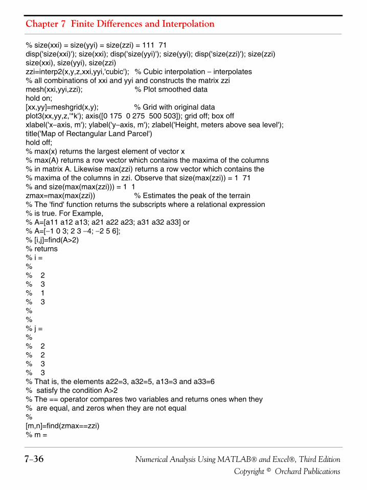
Chapter 7 Finite Differences and Interpolation
7−36 Numerical Analysis Using MATLAB® and Excel®, Third EditionCopyright © Orchard Publications
% size(xxi) = size(yyi) = size(zzi) = 111 71disp('size(xxi)'); size(xxi); disp('size(yyi)'); size(yyi); disp('size(zzi)'); size(zzi)size(xxi), size(yyi), size(zzi)zzi=interp2(x,y,z,xxi,yyi,'cubic'); % Cubic interpolation − interpolates% all combinations of xxi and yyi and constructs the matrix zzimesh(xxi,yyi,zzi); % Plot smoothed datahold on;[xx,yy]=meshgrid(x,y); % Grid with original dataplot3(xx,yy,z,'*k'); axis([0 175 0 275 500 503]); grid off; box offxlabel('x−axis, m'); ylabel('y−axis, m'); zlabel('Height, meters above sea level');title('Map of Rectangular Land Parcel')hold off;% max(x) returns the largest element of vector x% max(A) returns a row vector which contains the maxima of the columns% in matrix A. Likewise max(zzi) returns a row vector which contains the% maxima of the columns in zzi. Observe that size(max(zzi)) = 1 71% and size(max(max(zzi))) = 1 1zmax=max(max(zzi)) % Estimates the peak of the terrain% The 'find' function returns the subscripts where a relational expression% is true. For Example,% A=[a11 a12 a13; a21 a22 a23; a31 a32 a33] or% A=[−1 0 3; 2 3 −4; −2 5 6];% [i,j]=find(A>2)% returns% i =%% 2% 3% 1% 3%%% j =%% 2% 2% 3% 3% That is, the elements a22=3, a32=5, a13=3 and a33=6 % satisfy the condition A>2% The == operator compares two variables and returns ones when they% are equal, and zeros when they are not equal%[m,n]=find(zmax==zzi)% m =
Numerical Analysis Using MATLAB® and Excel®, Third Edition 7−37Copyright © Orchard Publications
Interpolation with MATLAB
%% 65%% n =%% 36%% that is, zmax is located at zzi = Z(65)(36)%% the x−cordinate is found fromxmax=xi(n)% xmax =%% 1.7500 % Column 36; size(xi) = 1 71% and the y−coordinate is found fromymax=yi(m)% ymax =%% 3.2000 % Row 65; size(yi) = 1 111% Remember that i is the row index, j is the column index, and x−axis % varies across the rows of z and y−axis varies down the columns of z
Interpolated z is:z_int = 500.1492
size(xi)
ans = 1 71
size(yi)
ans = 1 111
size(xxi)
ans = 111 71
size(yyi)
ans = 111 71
zzi=interp2(x,y,z,xxi,yyi,'cubic'); % Cubic interpolation − interpolates% all combinations of xxi and yyi and constructs the matrix zzi
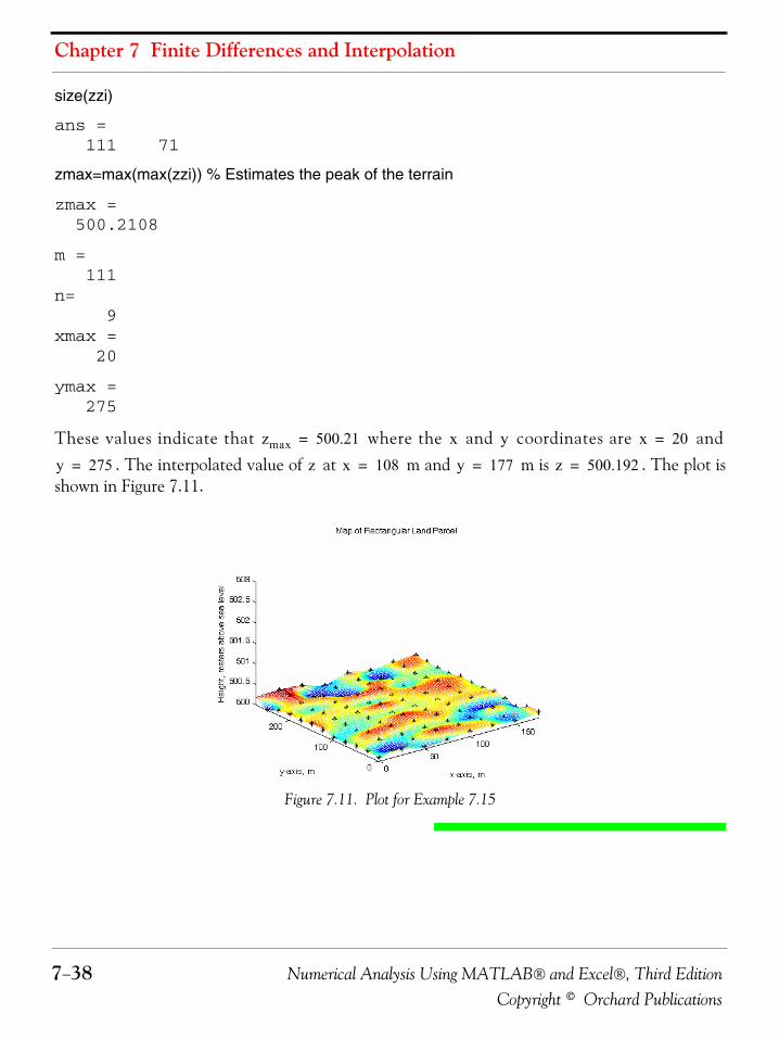
Chapter 7 Finite Differences and Interpolation
7−38 Numerical Analysis Using MATLAB® and Excel®, Third EditionCopyright © Orchard Publications
size(zzi)
ans = 111 71
zmax=max(max(zzi)) % Estimates the peak of the terrain
zmax = 500.2108
m = 111n= 9xmax = 20
ymax = 275
These values indicate that where the and coordinates are and. The interpolated value of at m and m is . The plot is
shown in Figure 7.11.
Figure 7.11. Plot for Example 7.15
zmax 500.21= x y x 20=
y 275= z x 108= y 177= z 500.192=
Numerical Analysis Using MATLAB® and Excel®, Third Edition 7−39Copyright © Orchard Publications
Summary
7.9 Summary• The first divided difference is defined as:
where and are any two, not necessarily consecutive values of , within an interval.
• Likewise, the second divided difference is defined as:
and the third, fourth, and so on divided differences are defined similarly.
• If the values of are equally spaced and the denominators are all the same, these values arereferred to as the differences of the function.
• If the constant difference between successive values of is , the typical value of is
• We can now express the first differences are usually expressed in terms of the difference oper-ator as
• Likewise, the second differences are expressed as
and, in general, for positive integer values of
• The difference operator obeys the law of exponents which states that
• The differences are found from the relation
For , and , the above relation reduces to
f xi xj,( )f xi( ) f xj( )–
xi xj–-----------------------------=
xi xj x
f xi xj xk, ,( )f xi xj,( ) f xj xk,( )–
xi xk–---------------------------------------------=
x
x h xk
xk x0 kh for k+ … 2 1 0 1 2 …, , , ,–,–,= =
ΔΔfk fk 1+ fk–=
Δ2fk Δ Δfk( ) Δfk 1+ Δfk–= =
n
Δnfk Δ Δn 1– fk( ) Δn 1– fk 1+ Δn 1– fk–= =
Δ
Δm Δnfk( ) Δm n+ fk=
nth Δnfk
Δnfk fk n+ nfk n 1–+–n n 1–( )
2!--------------------fk n 2–+ … 1–( )n 1– nfk 1+ 1–( )nfk+ + + +=
k 0= n 1 2 3, ,= 4
Chapter 7 Finite Differences and Interpolation
7−40 Numerical Analysis Using MATLAB® and Excel®, Third EditionCopyright © Orchard Publications
• As with derivatives, the differences of a polynomial of degree are constant.
• The factorial polynomials are defined as
and
Using the difference operator with the above relations we obtain
and
These are very similar to differentiation of and .
• We can express any algebraic polynomial as a factorial polynomial . Then, in anal-ogy with Maclaurin power series, we can express that polynomial as
where
• Factorial polynomials provide an easier method of constructing a difference table. The proce-dure is as follows:
1. We divide by to obtain a quotient and a remainder which turns out to be
the constant term . Then, the factorial polynomial reduces to
Δf0 f2 f1–=
Δ2f0 f2 2f1– f0+=
Δ3f0 f3 3f2– 3f1 f0–+=
Δ4f0 f4 4f3 6f2 4– f1 f0+ +–=
nth n
x( ) n( ) x x 1–( ) x 2–( )… x n– 1+( )=
x( ) n( )– 1x 1–( ) x 2–( )… x n+( )
----------------------------------------------------------=
Δ
Δ x( ) n( ) n x( ) n 1–( )=
Δ x( ) n( )– n– x( ) n 1–( )–=
xn x n–
fn x( ) pn x( )
pn x( ) a0 a1 x( ) 1( ) a2 x( ) 2( ) … an x( ) n( )+ + + +=
ajΔjpn 0( )
j!------------------- for j 0 1 2 … n, , , ,= =
pn x( ) x q0 x( ) r0
a0
pn x( ) r0 xq0 x( )+=
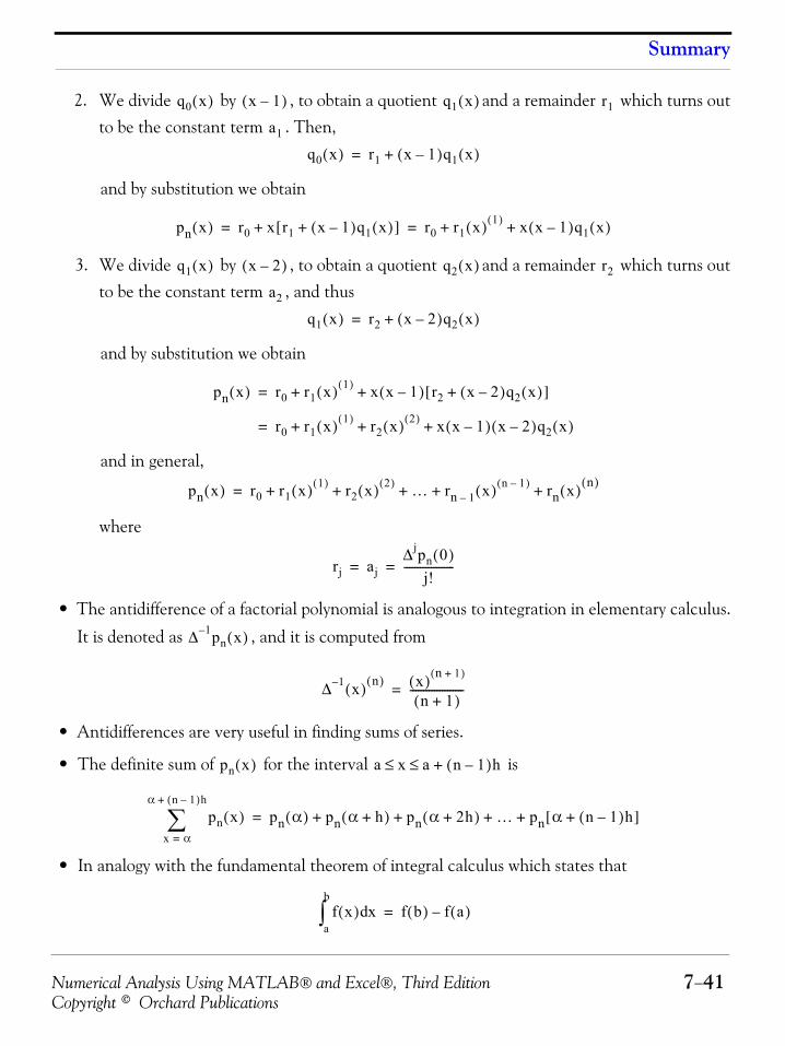
Numerical Analysis Using MATLAB® and Excel®, Third Edition 7−41Copyright © Orchard Publications
Summary
2. We divide by , to obtain a quotient and a remainder which turns outto be the constant term . Then,
and by substitution we obtain
3. We divide by , to obtain a quotient and a remainder which turns outto be the constant term , and thus
and by substitution we obtain
and in general,
where
• The antidifference of a factorial polynomial is analogous to integration in elementary calculus.
It is denoted as , and it is computed from
• Antidifferences are very useful in finding sums of series.
• The definite sum of for the interval is
• In analogy with the fundamental theorem of integral calculus which states that
q0 x( ) x 1–( ) q1 x( ) r1
a1
q0 x( ) r1 x 1–( )q1 x( )+=
pn x( ) r0 x r1 x 1–( )q1 x( )+[ ]+ r0 r1 x( ) 1( ) x x 1–( )q1 x( )+ += =
q1 x( ) x 2–( ) q2 x( ) r2
a2
q1 x( ) r2 x 2–( )q2 x( )+=
pn x( ) r0 r1 x( ) 1( ) x x 1–( ) r2 x 2–( )q2 x( )+[ ]+ +=
r0 r1 x( ) 1( )+ r2 x( ) 2( ) x x 1–( ) x 2–( )q2 x( )+ +=
pn x( ) r0 r1 x( ) 1( )+ r2 x( ) 2( ) … rn 1– x( ) n 1–( ) rn x( ) n( )+ + + +=
rj ajΔjpn 0( )
j!-------------------= =
Δ 1– pn x( )
Δ 1– x( ) n( ) x( ) n 1+( )
n 1+( )--------------------=
pn x( ) a x a n 1–( )h+≤ ≤
pn x( )x α=
α n 1–( )h+
∑ pn α( ) pn α h+( ) pn α 2h+( ) … pn α n 1–( )h+[ ]+ + + +=
f x( ) xda
b
∫ f b( ) f a( )–=
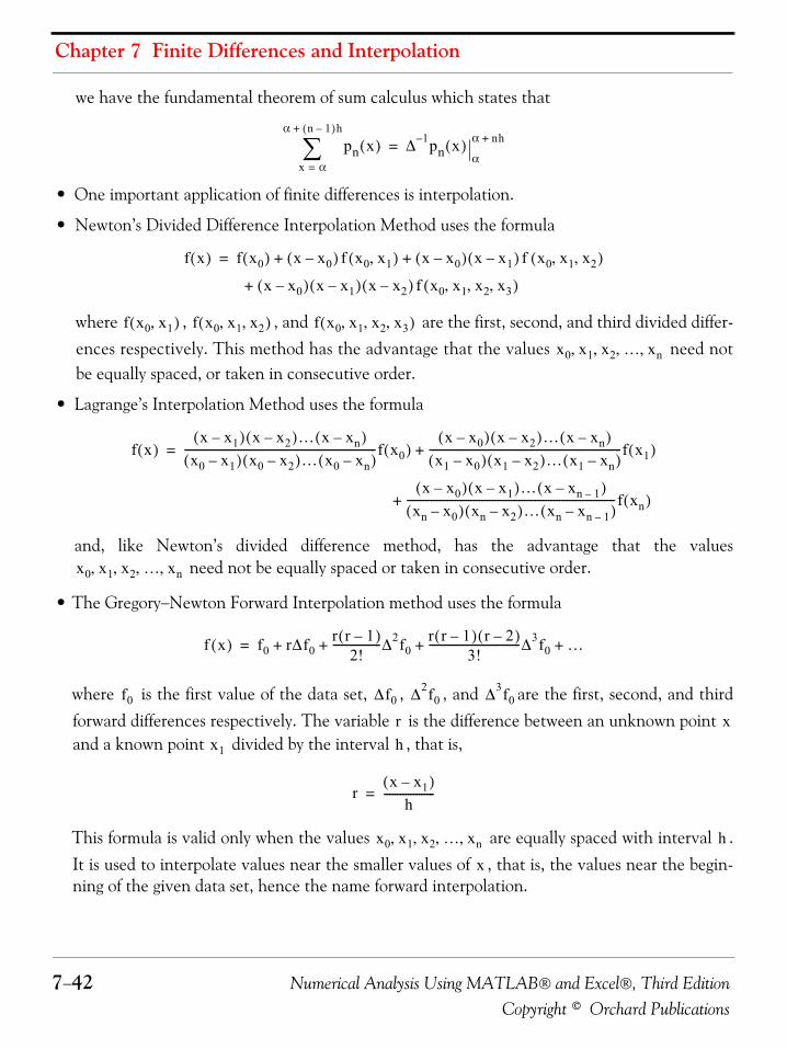
Chapter 7 Finite Differences and Interpolation
7−42 Numerical Analysis Using MATLAB® and Excel®, Third EditionCopyright © Orchard Publications
we have the fundamental theorem of sum calculus which states that
• One important application of finite differences is interpolation.
• Newton’s Divided Difference Interpolation Method uses the formula
where , , and are the first, second, and third divided differ-ences respectively. This method has the advantage that the values need notbe equally spaced, or taken in consecutive order.
• Lagrange’s Interpolation Method uses the formula
and, like Newton’s divided difference method, has the advantage that the values need not be equally spaced or taken in consecutive order.
• The Gregory−Newton Forward Interpolation method uses the formula
where is the first value of the data set, , , and are the first, second, and thirdforward differences respectively. The variable is the difference between an unknown point and a known point divided by the interval , that is,
This formula is valid only when the values are equally spaced with interval .It is used to interpolate values near the smaller values of , that is, the values near the begin-ning of the given data set, hence the name forward interpolation.
pn x( )x α=
α n 1–( )h+
∑ Δ 1– pn x( )α
α nh+=
f x( ) f x0( ) x x0–( ) f x0 x1,( ) x x0–( ) x x1–( ) f x0 x1 x2, ,( )+ +=
x x0–( ) x x1–( ) x x2–( ) f x0 x1 x2 x3, , ,( )+
f x0 x1,( ) f x0 x1 x2, ,( ) f x0 x1 x2 x3, , ,( )
x0 x1 x2 … xn, , , ,
f x( )x x1–( ) x x2–( )… x xn–( )
x0 x1–( ) x0 x2–( )… x0 xn–( )------------------------------------------------------------------------f x0( )
x x0–( ) x x2–( )… x xn–( )x1 x0–( ) x1 x2–( )… x1 xn–( )
------------------------------------------------------------------------f x1( )+=
x x0–( ) x x1–( )… x xn 1––( )
xn x0–( ) xn x2–( )… xn xn 1––( )------------------------------------------------------------------------------f xn( )+
x0 x1 x2 … xn, , , ,
f x( ) f0 rΔf0r r 1–( )
2!------------------Δ2f0
r r 1–( ) r 2–( )3!
----------------------------------Δ3f0 …+ + + +=
f0 Δf0 Δ2f0 Δ3f0
r xx1 h
rx x1–( )
h-------------------=
x0 x1 x2 … xn, , , , h
x
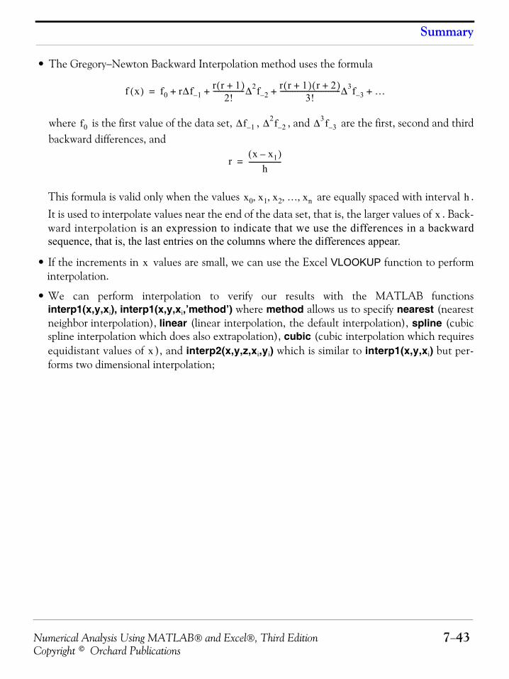
Numerical Analysis Using MATLAB® and Excel®, Third Edition 7−43Copyright © Orchard Publications
Summary
• The Gregory−Newton Backward Interpolation method uses the formula
where is the first value of the data set, , , and are the first, second and thirdbackward differences, and
This formula is valid only when the values are equally spaced with interval .It is used to interpolate values near the end of the data set, that is, the larger values of . Back-ward interpolation is an expression to indicate that we use the differences in a backwardsequence, that is, the last entries on the columns where the differences appear.
• If the increments in values are small, we can use the Excel VLOOKUP function to performinterpolation.
• We can perform interpolation to verify our results with the MATLAB functionsinterp1(x,y,xi), interp1(x,y,xi,’method’) where method allows us to specify nearest (nearestneighbor interpolation), linear (linear interpolation, the default interpolation), spline (cubicspline interpolation which does also extrapolation), cubic (cubic interpolation which requiresequidistant values of ), and interp2(x,y,z,xi,yi) which is similar to interp1(x,y,xi) but per-forms two dimensional interpolation;
f x( ) f0 rΔf 1–r r 1+( )
2!------------------Δ2f 2–
r r 1+( ) r 2+( )3!
-----------------------------------Δ3f 3– …+ + + +=
f0 Δf 1– Δ2f 2– Δ3f 3–
rx x1–( )
h-------------------=
x0 x1 x2 … xn, , , , h
x
x
x
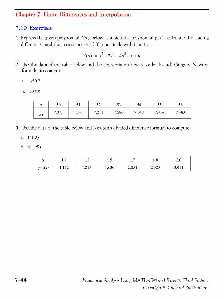
Chapter 7 Finite Differences and Interpolation
7−44 Numerical Analysis Using MATLAB® and Excel®, Third EditionCopyright © Orchard Publications
7.10 Exercises
1. Express the given polynomial below as a factorial polynomial , calculate the leadingdifferences, and then construct the difference table with .
2. Use the data of the table below and the appropriate (forward or backward) Gregory−Newtonformula, to compute:
a.
b.
3. Use the data of the table below and Newton’s divided difference formula to compute:
a.
b.
x 50 51 52 53 54 55 56
7.071 7.141 7.211 7.280 7.348 7.416 7.483
x 1.1 1.2 1.5 1.7 1.8 2.0
y=f(x) 1.112 1.219 1.636 2.054 2.323 3.011
f x( ) p x( )h 1=
f x( ) x5 2x4 4x3+– x– 6+=
50.2
55.9
x
f 1.3( )
f 1.95( )
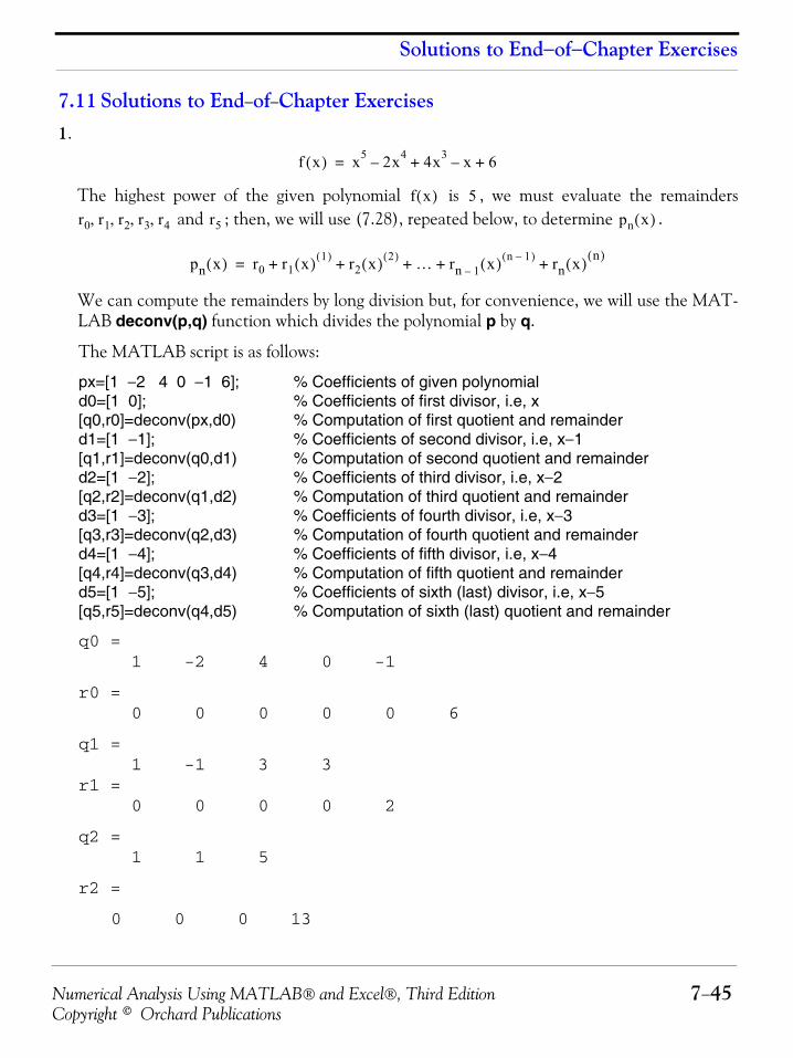
Numerical Analysis Using MATLAB® and Excel®, Third Edition 7−45Copyright © Orchard Publications
Solutions to End−of−Chapter Exercises
7.11 Solutions to End−of−Chapter Exercises1.
The highest power of the given polynomial is , we must evaluate the remainders and ; then, we will use (7.28), repeated below, to determine .
We can compute the remainders by long division but, for convenience, we will use the MAT-LAB deconv(p,q) function which divides the polynomial p by q.
The MATLAB script is as follows:
px=[1 −2 4 0 −1 6]; % Coefficients of given polynomiald0=[1 0]; % Coefficients of first divisor, i.e, x[q0,r0]=deconv(px,d0) % Computation of first quotient and remainderd1=[1 −1]; % Coefficients of second divisor, i.e, x−1[q1,r1]=deconv(q0,d1) % Computation of second quotient and remainderd2=[1 −2]; % Coefficients of third divisor, i.e, x−2[q2,r2]=deconv(q1,d2) % Computation of third quotient and remainderd3=[1 −3]; % Coefficients of fourth divisor, i.e, x−3[q3,r3]=deconv(q2,d3) % Computation of fourth quotient and remainderd4=[1 −4]; % Coefficients of fifth divisor, i.e, x−4[q4,r4]=deconv(q3,d4) % Computation of fifth quotient and remainderd5=[1 −5]; % Coefficients of sixth (last) divisor, i.e, x−5[q5,r5]=deconv(q4,d5) % Computation of sixth (last) quotient and remainder
q0 = 1 -2 4 0 -1
r0 = 0 0 0 0 0 6
q1 = 1 -1 3 3r1 = 0 0 0 0 2
q2 = 1 1 5
r2 =
0 0 0 13
f x( ) x5 2x4 4x3+– x– 6+=
f x( ) 5r0 r1 r2 r3 r4, , , , r5 pn x( )
pn x( ) r0 r1 x( ) 1( )+ r2 x( ) 2( ) … rn 1– x( ) n 1–( ) rn x( ) n( )+ + + +=
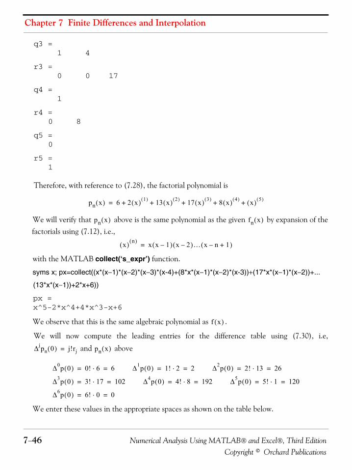
Chapter 7 Finite Differences and Interpolation
7−46 Numerical Analysis Using MATLAB® and Excel®, Third EditionCopyright © Orchard Publications
q3 = 1 4
r3 = 0 0 17
q4 = 1
r4 = 0 8
q5 = 0
r5 = 1
Therefore, with reference to (7.28), the factorial polynomial is
We will verify that above is the same polynomial as the given by expansion of thefactorials using (7.12), i.e.,
with the MATLAB collect(‘s_expr’) function.
syms x; px=collect((x*(x−1)*(x−2)*(x−3)*(x-4)+(8*x*(x−1)*(x−2)*(x-3))+(17*x*(x−1)*(x−2))+...
(13*x*(x−1))+2*x+6))
px = x^5-2*x^4+4*x^3-x+6
We observe that this is the same algebraic polynomial as .
We will now compute the leading entries for the difference table using (7.30), i.e,
and above
We enter these values in the appropriate spaces as shown on the table below.
pn x( ) 6 2 x( ) 1( ) 13 x( ) 2( ) 17 x( ) 3( ) 8 x( ) 4( ) x( ) 5( )+ + + + +=
pn x( ) fn x( )
x( ) n( ) x x 1–( ) x 2–( )… x n– 1+( )=
f x( )
Δjpn 0( ) j!rj= pn x( )
Δ0p 0( ) 0! 6⋅ 6= = Δ1p 0( ) 1! 2⋅ 2= = Δ2p 0( ) 2! 13⋅ 26= =
Δ3p 0( ) 3! 17⋅ 102= = Δ4p 0( ) 4! 8⋅ 192= = Δ5p 0( ) 5! 1⋅ 120= =
Δ6p 0( ) 6! 0⋅ 0= =
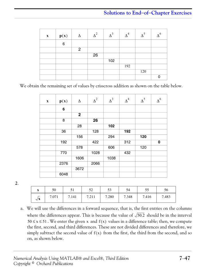
Numerical Analysis Using MATLAB® and Excel®, Third Edition 7−47Copyright © Orchard Publications
Solutions to End−of−Chapter Exercises
We obtain the remaining set of values by crisscross addition as shown on the table below.
2.
a. We will use the differences in a forward sequence, that is, the first entries on the columnswhere the differences appear. This is because the value of should be in the interval
. We enter the given and values in a difference table; then, we computethe first, second, and third differences. These are not divided differences and therefore, wesimply subtract the second value of from the first, the third from the second, and soon, as shown below.
62
26102
192120
0
62
8 2628 102
36 128 192156 294 120
192 422 312 0578 606 120
770 1028 4321606 1038
2376 20663672
6048
x 50 51 52 53 54 55 56
7.071 7.141 7.211 7.280 7.348 7.416 7.483
x p x( ) Δ Δ2 Δ3 Δ4 Δ5 Δ6
x p x( ) Δ Δ2 Δ3 Δ4 Δ5 Δ6
x
50.250 x 51≤ ≤ x f x( )
f x( )
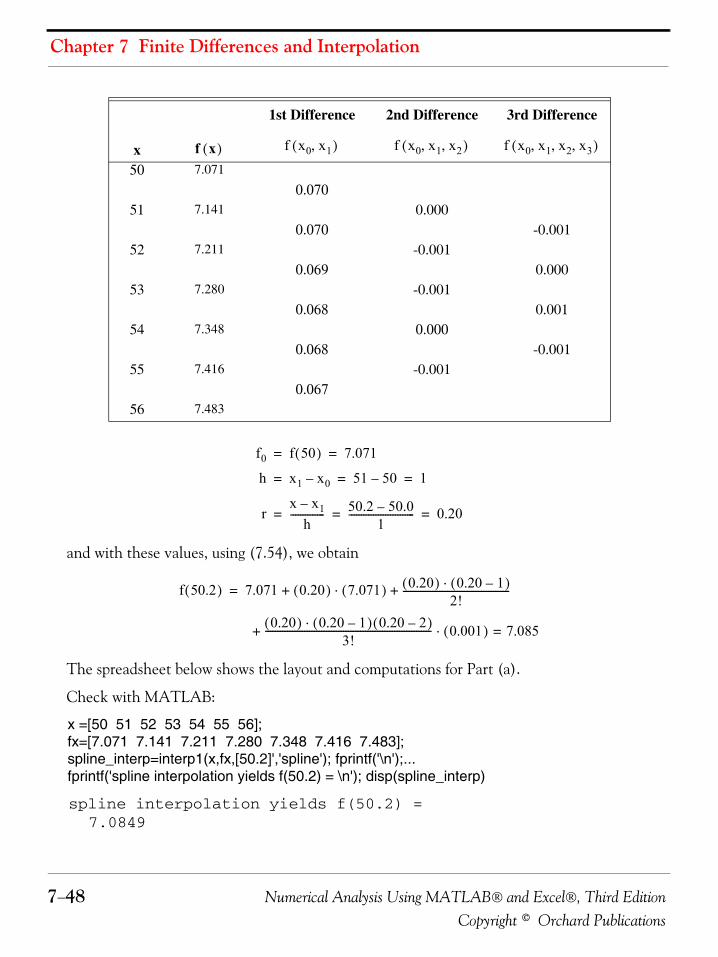
Chapter 7 Finite Differences and Interpolation
7−48 Numerical Analysis Using MATLAB® and Excel®, Third EditionCopyright © Orchard Publications
and with these values, using (7.54), we obtain
The spreadsheet below shows the layout and computations for Part (a).
Check with MATLAB:
x =[50 51 52 53 54 55 56];fx=[7.071 7.141 7.211 7.280 7.348 7.416 7.483];spline_interp=interp1(x,fx,[50.2]','spline'); fprintf('\n');...fprintf('spline interpolation yields f(50.2) = \n'); disp(spline_interp)
spline interpolation yields f(50.2) = 7.0849
1st Difference 2nd Difference 3rd Difference
x50 7.071
0.07051 7.141 0.000
0.070 -0.00152 7.211 -0.001
0.069 0.00053 7.280 -0.001
0.068 0.00154 7.348 0.000
0.068 -0.00155 7.416 -0.001
0.06756 7.483
f x( ) f x0 x1,( ) f x0 x1 x2, ,( ) f x0 x1 x2 x3, , ,( )
f0 f 50( ) 7.071= =
h x1 x0– 51 50– 1= = =
rx x1–
h-------------- 50.2 50.0–
1--------------------------- 0.20= = =
f 50.2( ) 7.071 0.20( ) 7.071( )⋅ 0.20( ) 0.20 1–( )⋅2!
--------------------------------------------+ +=
0.20( ) 0.20 1–( ) 0.20 2–( )⋅3!
-------------------------------------------------------------------- 0.001( )⋅ 7.085=+
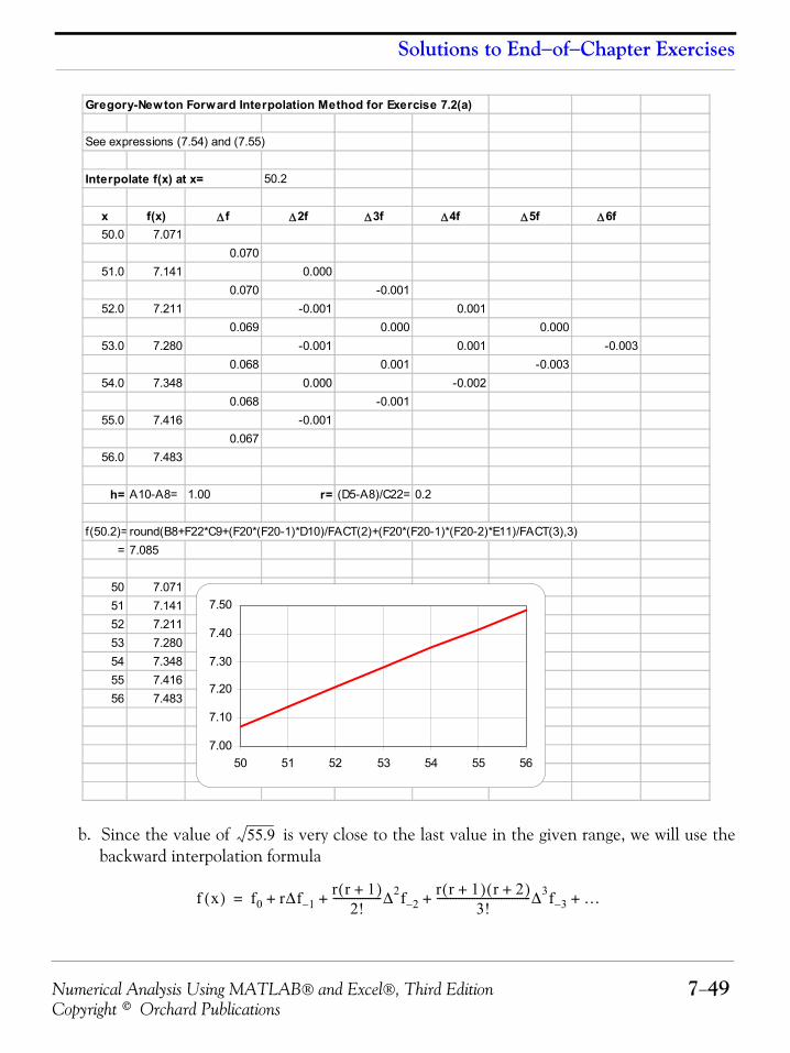
Numerical Analysis Using MATLAB® and Excel®, Third Edition 7−49Copyright © Orchard Publications
Solutions to End−of−Chapter Exercises
b. Since the value of is very close to the last value in the given range, we will use thebackward interpolation formula
Gregory-Newton Forward Interpolation Method for Exercise 7.2(a)
See expressions (7.54) and (7.55)
Interpolate f(x) at x= 50.2
x f(x) Δ f Δ2f Δ3f Δ4f Δ5f Δ6f50.0 7.071
0.07051.0 7.141 0.000
0.070 -0.00152.0 7.211 -0.001 0.001
0.069 0.000 0.00053.0 7.280 -0.001 0.001 -0.003
0.068 0.001 -0.00354.0 7.348 0.000 -0.002
0.068 -0.00155.0 7.416 -0.001
0.06756.0 7.483
h= A10-A8= 1.00 r= (D5-A8)/C22= 0.2
f(50.2)= round(B8+F22*C9+(F20*(F20-1)*D10)/FACT(2)+(F20*(F20-1)*(F20-2)*E11)/FACT(3),3)= 7.085
50 7.07151 7.14152 7.21153 7.28054 7.34855 7.41656 7.483
7.00
7.10
7.20
7.30
7.40
7.50
50 51 52 53 54 55 56
55.9
f x( ) f0 rΔf 1–r r 1+( )
2!------------------Δ2f 2–
r r 1+( ) r 2+( )3!
-----------------------------------Δ3f 3– …+ + + +=
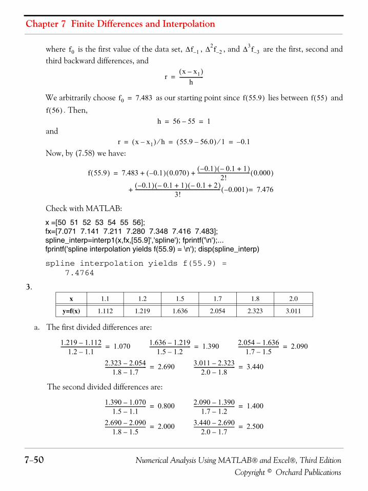
Chapter 7 Finite Differences and Interpolation
7−50 Numerical Analysis Using MATLAB® and Excel®, Third EditionCopyright © Orchard Publications
where is the first value of the data set, , , and are the first, second andthird backward differences, and
We arbitrarily choose as our starting point since lies between and. Then,
and
Now, by (7.58) we have:
Check with MATLAB:
x =[50 51 52 53 54 55 56];fx=[7.071 7.141 7.211 7.280 7.348 7.416 7.483];spline_interp=interp1(x,fx,[55.9]','spline'); fprintf('\n');...fprintf('spline interpolation yields f(55.9) = \n'); disp(spline_interp)
spline interpolation yields f(55.9) = 7.4764
3.
a. The first divided differences are:
The second divided differences are:
x 1.1 1.2 1.5 1.7 1.8 2.0
y=f(x) 1.112 1.219 1.636 2.054 2.323 3.011
f0 Δf 1– Δ2f 2– Δ3f 3–
rx x1–( )
h-------------------=
f0 7.483= f 55.9( ) f 55( )
f 56( )h 56 55– 1= =
r x x1–( ) h⁄ 55.9 56.0–( ) 1⁄ 0.1–= = =
f 55.9( ) 7.483 0.1–( ) 0.070( ) 0.1–( ) 0.1– 1+( )2!
------------------------------------------ 0.000( )
0.1–( ) 0.1– 1+( ) 0.1– 2+( )3!
-------------------------------------------------------------------- 0.001–( ) 7.476=
+ +
+
=
1.219 1.112–1.2 1.1–
--------------------------------- 1.070= 1.636 1.219–1.5 1.2–
--------------------------------- 1.390= 2.054 1.636–1.7 1.5–
--------------------------------- 2.090=
2.323 2.054–1.8 1.7–
--------------------------------- 2.690= 3.011 2.323–2.0 1.8–
--------------------------------- 3.440=
1.390 1.070–1.5 1.1–
--------------------------------- 0.800= 2.090 1.390–1.7 1.2–
--------------------------------- 1.400=
2.690 2.090–1.8 1.5–
--------------------------------- 2.000= 3.440 2.690–2.0 1.7–
--------------------------------- 2.500=
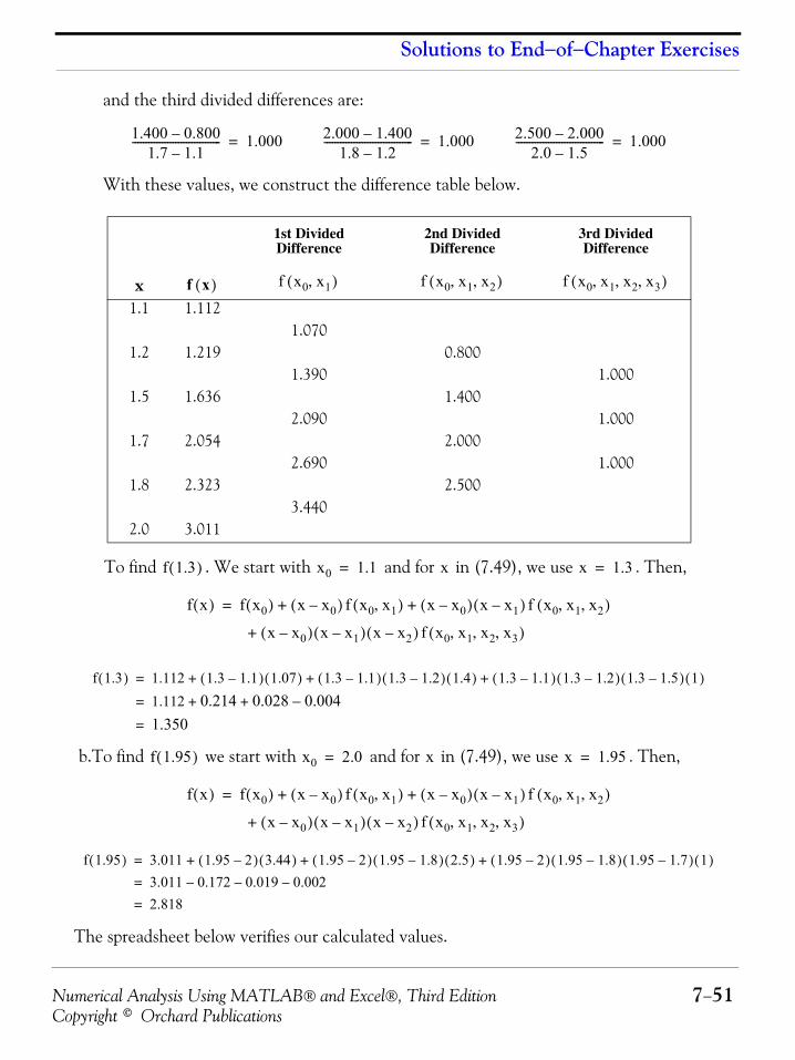
Numerical Analysis Using MATLAB® and Excel®, Third Edition 7−51Copyright © Orchard Publications
Solutions to End−of−Chapter Exercises
and the third divided differences are:
With these values, we construct the difference table below.
To find . We start with and for in (7.49), we use . Then,
b.To find we start with and for in (7.49), we use . Then,
The spreadsheet below verifies our calculated values.
1st Divided Difference
2nd Divided Difference
3rd Divided Difference
x1.1 1.112
1.0701.2 1.219 0.800
1.390 1.0001.5 1.636 1.400
2.090 1.0001.7 2.054 2.000
2.690 1.0001.8 2.323 2.500
3.4402.0 3.011
1.400 0.800–1.7 1.1–
--------------------------------- 1.000= 2.000 1.400–1.8 1.2–
--------------------------------- 1.000= 2.500 2.000–2.0 1.5–
--------------------------------- 1.000=
f x( ) f x0 x1,( ) f x0 x1 x2, ,( ) f x0 x1 x2 x3, , ,( )
f 1.3( ) x0 1.1= x x 1.3=
f x( ) f x0( ) x x0–( ) f x0 x1,( ) x x0–( ) x x1–( ) f x0 x1 x2, ,( )+ +=
x x0–( ) x x1–( ) x x2–( ) f x0 x1 x2 x3, , ,( )+
f 1.3( ) 1.112 1.3 1.1–( ) 1.07( ) 1.3 1.1–( ) 1.3 1.2–( ) 1.4( ) 1.3 1.1–( ) 1.3 1.2–( ) 1.3 1.5–( ) 1( )+ + +=
1.112 0.214 0.028 0.004–+ +=
1.350=
f 1.95( ) x0 2.0= x x 1.95=
f x( ) f x0( ) x x0–( ) f x0 x1,( ) x x0–( ) x x1–( ) f x0 x1 x2, ,( )+ +=
x x0–( ) x x1–( ) x x2–( ) f x0 x1 x2 x3, , ,( )+
f 1.95( ) 3.011 1.95 2–( ) 3.44( ) 1.95 2–( ) 1.95 1.8–( ) 2.5( ) 1.95 2–( ) 1.95 1.8–( ) 1.95 1.7–( ) 1( )+ + +=
3.011 0.172– 0.019– 0.002–=
2.818=
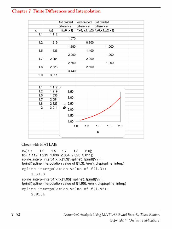
Chapter 7 Finite Differences and Interpolation
7−52 Numerical Analysis Using MATLAB® and Excel®, Third EditionCopyright © Orchard Publications
Check with MATLAB:
x=[ 1.1 1.2 1.5 1.7 1.8 2.0];fx=[ 1.112 1.219 1.636 2.054 2.323 3.011];spline_interp=interp1(x,fx,[1.3]','spline'); fprintf('\n');...fprintf('spline interpolation value of f(1.3): \n\n'); disp(spline_interp)spline interpolation value of f(1.3):
1.3380
spline_interp=interp1(x,fx,[1.95]','spline'); fprintf('\n');...fprintf('spline interpolation value of f(1.95): \n\n'); disp(spline_interp)spline interpolation value of f(1.95):
2.8184
1st divided 2nd divided 3rd divideddifference difference difference
x f(x) f(x0, x1) f(x0, x1, x2) f(x0,x1,x2,x3)1.1 1.112
1.0701.2 1.219 0.800
1.390 1.0001.5 1.636 1.400
2.090 1.0001.7 2.054 2.000
2.690 1.0001.8 2.323 2.500
3.4402.0 3.011
1.1 1.1121.2 1.2191.5 1.6361.7 2.0541.8 2.323
2 3.011
1.00
1.50
2.00
2.50
3.00
3.50
1.0 1.3 1.5 1.8 2.0
x
f(x)
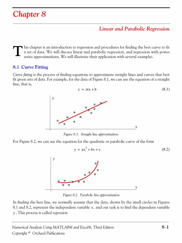
Numerical Analysis Using MATLAB® and Excel®, Third Edition 8−1Copyright © Orchard Publications
Chapter 8
Linear and Parabolic Regression
his chapter is an introduction to regression and procedures for finding the best curve to fita set of data. We will discuss linear and parabolic regression, and regression with powerseries approximations. We will illustrate their application with several examples.
8.1 Curve FittingCurve fitting is the process of finding equations to approximate straight lines and curves that bestfit given sets of data. For example, for the data of Figure 8.1, we can use the equation of a straightline, that is,
(8.1)
Figure 8.1. Straight line approximation.
For Figure 8.2, we can use the equation for the quadratic or parabolic curve of the form
(8.2)
Figure 8.2. Parabolic line approximation
In finding the best line, we normally assume that the data, shown by the small circles in Figures8.1 and 8.2, represent the independent variable , and our task is to find the dependent variable
. This process is called regression.
T
y mx b+=
y
x
y ax2 bx c+ +=
y
x
xy
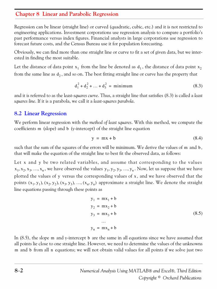
Chapter 8 Linear and Parabolic Regression
8−2 Numerical Analysis Using MATLAB® and Excel®, Third EditionCopyright © Orchard Publications
Regression can be linear (straight line) or curved (quadratic, cubic, etc.) and it is not restricted toengineering applications. Investment corporations use regression analysis to compare a portfolio’spast performance versus index figures. Financial analysts in large corporations use regression toforecast future costs, and the Census Bureau use it for population forecasting.
Obviously, we can find more than one straight line or curve to fit a set of given data, but we inter-ested in finding the most suitable.
Let the distance of data point from the line be denoted as , the distance of data point from the same line as , and so on. The best fitting straight line or curve has the property that
(8.3)
and it is referred to as the least-squares curve. Thus, a straight line that satisfies (8.3) is called a leastsquares line. If it is a parabola, we call it a least-squares parabola.
8.2 Linear RegressionWe perform linear regression with the method of least squares. With this method, we compute thecoefficients (slope) and (y-intercept) of the straight line equation
(8.4)
such that the sum of the squares of the errors will be minimum. We derive the values of and ,that will make the equation of the straight line to best fit the observed data, as follows:
Let and be two related variables, and assume that corresponding to the values, we have observed the values . Now, let us suppose that we have
plotted the values of versus the corresponding values of , and we have observed that thepoints approximate a straight line. We denote the straightline equations passing through these points as
(8.5)
In (8.5), the slope and y-intercept are the same in all equations since we have assumed thatall points lie close to one straight line. However, we need to determine the values of the unknowns
and from all equations; we will not obtain valid values for all points if we solve just two
x1 d1 x2
d2
d12 d2
2 … d32+ + + minimum=
m b
y mx b+=
m b
x yx1 x2 x3 … xn, , , , y1 y2 y3 … yn, , , ,
y xx1 y1,( ) x2 y2,( ) x3 y3,( ) … xn yn,( ), , , ,
y1 mx1 b+=
y2 mx2 b+=
y3 mx3 b+=
…yn mxn b+=
m b
m b n
Numerical Analysis Using MATLAB® and Excel®, Third Edition 8−3Copyright © Orchard Publications
Linear Regression
equations with two unknowns. *
The error (difference) between the observed value , and the value that lies on the straight line,is . This difference could be positive or negative, depending on the position of theobserved value, and the value at the point on the straight line. Likewise, the error between theobserved value and the value that lies on the straight line is and so on. Thestraight line that we choose must be a straight line such that the distances between the observedvalues, and the corresponding values on the straight line, will be minimum. This will be achievedif we use the magnitudes (absolute values) of the distances; if we were to combine positive andnegative values, some may cancel each other and give us an erroneous sum of the distances.Accordingly, we find the sum of the squared distances between observed points and the points onthe straight line. For this reason, this method is referred to as the method of least squares.
Let the sum of the squares of the errors be
(8.6)
Since is a function of two variables and , to minimize (8.6) we must equate to
zero its two partial derivatives with respect to and . Then,
(8.7)
and
(8.8)
The second derivatives of (8.7) and (8.8) are positive and thus will have its minimum
value.
Collecting like terms, and simplifying (8.7) and (8.8) we obtain
* A linear system of independent equations that has more equations than unknowns is said to be overdetermined and noexact solution exists. On the contrary, a system that has more unknowns than equations is said to be underdetermined andthese systems have infinite solutions.
y1
y1 mx1 b+( )–
y2 y2 mx2 b+( )–
squares∑ y1 mx1 b+( )–[ ]2 y2 mx2 b+( )–[ ]2 …
yn mxn b+( )–[ ]2
+ +
+
=
squares∑ m b
m b
m∂∂ squares∑ 2x1 y1 mx1 b+( )–[ ]– 2x2 y2 mx2 b+( )–[ ] …––=
2xn yn mxn b+( )–[ ]– 0=
b∂∂ squares∑ 2 y1 mx1 b+( )–[ ]– 2 y2 mx2 b+( )–[ ] …––=
2 yn mxn b+( )–[ ]– 0=
squares∑
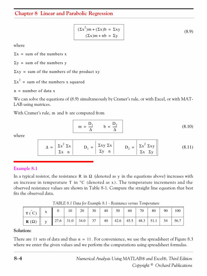
Chapter 8 Linear and Parabolic Regression
8−4 Numerical Analysis Using MATLAB® and Excel®, Third EditionCopyright © Orchard Publications
(8.9)
where
We can solve the equations of (8.9) simultaneously by Cramer’s rule, or with Excel, or with MAT-LAB using matrices.
With Cramer’s rule, and are computed from
(8.10)
where
(8.11)
Example 8.1
In a typical resistor, the resistance in (denoted as in the equations above) increases withan increase in temperature in (denoted as ). The temperature increments and theobserved resistance values are shown in Table 8-1. Compute the straight line equation that bestfits the observed data.
Solution:
There are sets of data and thus . For convenience, we use the spreadsheet of Figure 8.3where we enter the given values and we perform the computations using spreadsheet formulas.
TABLE 8.1 Data for Example 8.1 - Resistance versus Temperature
T 0 10 20 30 40 50 60 70 80 90 100
R 27.6 31.0 34.0 37 40 42.6 45.5 48.3 51.1 54 56.7
Σx2( )m Σx( )b+ Σxy=
Σx( )m nb+ Σy=
Σx sum of the numbers x=
Σy sum of the numbers y=
Σxy sum of the numbers of the product xy=
Σx2 sum of the numbers x squared=
n number of data x=
m b
mD1Δ
------= bD2Δ
------=
Δ Σx2 ΣxΣx n
= D1Σxy ΣxΣy n
= D2Σx2 ΣxyΣx Σy
=
R Ω yT °C x
C°( ) x
Ω( ) y
11 n 11=
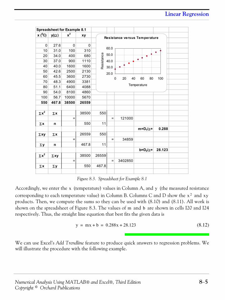
Numerical Analysis Using MATLAB® and Excel®, Third Edition 8−5Copyright © Orchard Publications
Linear Regression
Figure 8.3. Spreadsheet for Example 8.1
Accordingly, we enter the (temperature) values in Column A, and (the measured resistancecorresponding to each temperature value) in Column B. Columns C and D show the and products. Then, we compute the sums so they can be used with (8.10) and (8.11). All work isshown on the spreadsheet of Figure 8.3. The values of and are shown in cells I20 and I24respectively. Thus, the straight line equation that best fits the given data is
(8.12)
We can use Excel’s Add Trendline feature to produce quick answers to regression problems. Wewill illustrate the procedure with the following example.
Spreadsheet for Example 8.1x (0C) y(Ω ) x2 xy
0 27.6 0 010 31.0 100 31020 34.0 400 68030 37.0 900 111040 40.0 1600 160050 42.6 2500 213060 45.5 3600 273070 48.3 4900 338180 51.1 6400 408890 54.0 8100 4860
100 56.7 10000 5670550 467.8 38500 26559
Σ x2 Σ x 38500 550= = 121000
Σ x n 550 11m=D1/Δ= 0.288
Σ xy Σ x 26559 550= = 34859
Σ y n 467.8 11b=D2/Δ= 28.123
Σ x2 Σ xy 38500 26559= = 3402850
Σ x Σ y 550 467.8
Resistance versus Temperature
20.0
30.0
40.0
50.0
60.0
0 20 40 60 80 100
Temperature
Res
ista
nce
x yx 2 xy
m b
y mx b+ 0.288x 28.123+= =
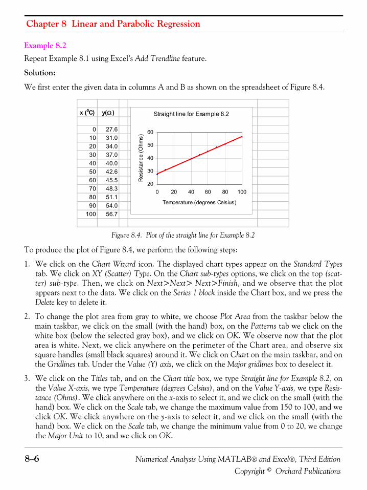
Chapter 8 Linear and Parabolic Regression
8−6 Numerical Analysis Using MATLAB® and Excel®, Third EditionCopyright © Orchard Publications
Example 8.2 Repeat Example 8.1 using Excel’s Add Trendline feature.
Solution:
We first enter the given data in columns A and B as shown on the spreadsheet of Figure 8.4.
Figure 8.4. Plot of the straight line for Example 8.2
To produce the plot of Figure 8.4, we perform the following steps:
1. We click on the Chart Wizard icon. The displayed chart types appear on the Standard Typestab. We click on XY (Scatter) Type. On the Chart sub-types options, we click on the top (scat-ter) sub-type. Then, we click on Next>Next> Next>Finish, and we observe that the plotappears next to the data. We click on the Series 1 block inside the Chart box, and we press theDelete key to delete it.
2. To change the plot area from gray to white, we choose Plot Area from the taskbar below themain taskbar, we click on the small (with the hand) box, on the Patterns tab we click on thewhite box (below the selected gray box), and we click on OK. We observe now that the plotarea is white. Next, we click anywhere on the perimeter of the Chart area, and observe sixsquare handles (small black squares) around it. We click on Chart on the main taskbar, and onthe Gridlines tab. Under the Value (Y) axis, we click on the Major gridlines box to deselect it.
3. We click on the Titles tab, and on the Chart title box, we type Straight line for Example 8.2, onthe Value X-axis, we type Temperature (degrees Celsius), and on the Value Y-axis, we type Resis-tance (Ohms). We click anywhere on the x-axis to select it, and we click on the small (with thehand) box. We click on the Scale tab, we change the maximum value from 150 to 100, and weclick OK. We click anywhere on the y-axis to select it, and we click on the small (with thehand) box. We click on the Scale tab, we change the minimum value from 0 to 20, we changethe Major Unit to 10, and we click on OK.
x (0C) y(Ω )
0 27.610 31.020 34.030 37.040 40.050 42.660 45.570 48.380 51.190 54.0
100 56.7
Straight line for Example 8.2
20
30
40
50
60
0 20 40 60 80 100
Temperature (degrees Celsius)
Res
ista
nce
(Ohm
s)
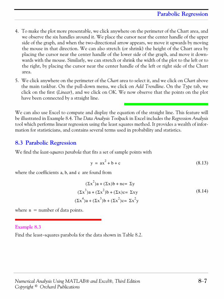
Numerical Analysis Using MATLAB® and Excel®, Third Edition 8−7Copyright © Orchard Publications
Parabolic Regression
4. To make the plot more presentable, we click anywhere on the perimeter of the Chart area, andwe observe the six handles around it. We place the cursor near the center handle of the upperside of the graph, and when the two-directional arrow appears, we move it upwards by movingthe mouse in that direction. We can also stretch (or shrink) the height of the Chart area byplacing the cursor near the center handle of the lower side of the graph, and move it down-wards with the mouse. Similarly, we can stretch or shrink the width of the plot to the left or tothe right, by placing the cursor near the center handle of the left or right side of the Chartarea.
5. We click anywhere on the perimeter of the Chart area to select it, and we click on Chart abovethe main taskbar. On the pull-down menu, we click on Add Trendline. On the Type tab, weclick on the first (Linear), and we click on OK. We now observe that the points on the plothave been connected by a straight line.
We can also use Excel to compute and display the equation of the straight line. This feature willbe illustrated in Example 8.4. The Data Analysis Toolpack in Excel includes the Regression Analysistool which performs linear regression using the least squares method. It provides a wealth of infor-mation for statisticians, and contains several terms used in probability and statistics.
8.3 Parabolic RegressionWe find the least-squares parabola that fits a set of sample points with
(8.13)
where the coefficients are found from
(8.14)
where = number of data points.
Example 8.3 Find the least−squares parabola for the data shown in Table 8.2.
y ax2 b c+ +=
a b and c, ,
Σx2( )a Σx( )b nc+ + Σy=
Σx3( )a Σx2( )b Σx( )c+ + Σxy=
Σx4( )a Σx3( )b Σx2( )c+ + Σx2y=
n
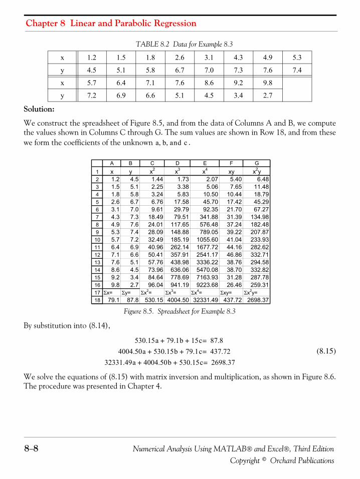
Chapter 8 Linear and Parabolic Regression
8−8 Numerical Analysis Using MATLAB® and Excel®, Third EditionCopyright © Orchard Publications
Solution:
We construct the spreadsheet of Figure 8.5, and from the data of Columns A and B, we computethe values shown in Columns C through G. The sum values are shown in Row 18, and from thesewe form the coefficients of the unknown .
Figure 8.5. Spreadsheet for Example 8.3
By substitution into (8.14),
(8.15)
We solve the equations of (8.15) with matrix inversion and multiplication, as shown in Figure 8.6.The procedure was presented in Chapter 4.
TABLE 8.2 Data for Example 8.3
x 1.2 1.5 1.8 2.6 3.1 4.3 4.9 5.3
y 4.5 5.1 5.8 6.7 7.0 7.3 7.6 7.4
x 5.7 6.4 7.1 7.6 8.6 9.2 9.8
y 7.2 6.9 6.6 5.1 4.5 3.4 2.7
a b and c, ,
123456789
101112131415161718
A B C D E F Gx y x2 x3 x4 xy x2y1.2 4.5 1.44 1.73 2.07 5.40 6.481.5 5.1 2.25 3.38 5.06 7.65 11.481.8 5.8 3.24 5.83 10.50 10.44 18.792.6 6.7 6.76 17.58 45.70 17.42 45.293.1 7.0 9.61 29.79 92.35 21.70 67.274.3 7.3 18.49 79.51 341.88 31.39 134.984.9 7.6 24.01 117.65 576.48 37.24 182.485.3 7.4 28.09 148.88 789.05 39.22 207.875.7 7.2 32.49 185.19 1055.60 41.04 233.936.4 6.9 40.96 262.14 1677.72 44.16 282.627.1 6.6 50.41 357.91 2541.17 46.86 332.717.6 5.1 57.76 438.98 3336.22 38.76 294.588.6 4.5 73.96 636.06 5470.08 38.70 332.829.2 3.4 84.64 778.69 7163.93 31.28 287.789.8 2.7 96.04 941.19 9223.68 26.46 259.31
Σx= Σy= Σx2= Σx3= Σx4= Σxy= Σx2y=79.1 87.8 530.15 4004.50 32331.49 437.72 2698.37
530.15a 79.1b 15c+ + 87.8=
4004.50a 530.15b 79.1c+ + 437.72=
32331.49a 4004.50b 530.15c+ + 2698.37=
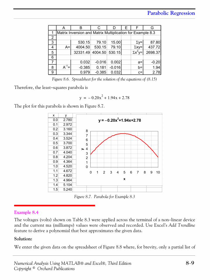
Numerical Analysis Using MATLAB® and Excel®, Third Edition 8−9Copyright © Orchard Publications
Parabolic Regression
Figure 8.6. Spreadsheet for the solution of the equations of (8.15)
Therefore, the least−squares parabola is
The plot for this parabola is shown in Figure 8.7.
Figure 8.7. Parabola for Example 8.3
Example 8.4 The voltages (volts) shown on Table 8.3 were applied across the terminal of a non−linear deviceand the current ma (milliamps) values were observed and recorded. Use Excel’s Add Trendlinefeature to derive a polynomial that best approximates the given data.
Solution:
We enter the given data on the spreadsheet of Figure 8.8 where, for brevity, only a partial list of
123456789
A B C D E F GMatrix Inversion and Matrix Multiplication for Example 8.3
530.15 79.10 15.00 Σy= 87.80A= 4004.50 530.15 79.10 Σxy= 437.72
32331.49 4004.50 530.15 Σx2y= 2698.37
0.032 -0.016 0.002 a= -0.20A-1= -0.385 0.181 -0.016 b= 1.94
0.979 -0.385 0.032 c= 2.78
y 0.20x2– 1.94x 2.78+ +=
x y0.0 2.7800.1 2.9720.2 3.1600.3 3.3440.4 3.5240.5 3.7000.6 3.8720.7 4.0400.8 4.2040.9 4.3641.0 4.5201.1 4.6721.2 4.8201.3 4.9641.4 5.1041.5 5.240
y = −0.20x2+1.94x+2.78
012345678
0 1 2 3 4 5 6 7 8 9 10
x
y
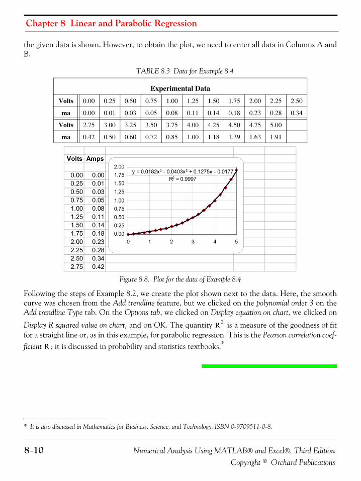
Chapter 8 Linear and Parabolic Regression
8−10 Numerical Analysis Using MATLAB® and Excel®, Third EditionCopyright © Orchard Publications
the given data is shown. However, to obtain the plot, we need to enter all data in Columns A andB.
Figure 8.8. Plot for the data of Example 8.4
Following the steps of Example 8.2, we create the plot shown next to the data. Here, the smoothcurve was chosen from the Add trendline feature, but we clicked on the polynomial order 3 on theAdd trendline Type tab. On the Options tab, we clicked on Display equation on chart, we clicked on
Display R squared value on chart, and on OK. The quantity is a measure of the goodness of fitfor a straight line or, as in this example, for parabolic regression. This is the Pearson correlation coef-ficient ; it is discussed in probability and statistics textbooks.*
TABLE 8.3 Data for Example 8.4
Experimental Data
Volts 0.00 0.25 0.50 0.75 1.00 1.25 1.50 1.75 2.00 2.25 2.50
ma 0.00 0.01 0.03 0.05 0.08 0.11 0.14 0.18 0.23 0.28 0.34
Volts 2.75 3.00 3.25 3.50 3.75 4.00 4.25 4.50 4.75 5.00
ma 0.42 0.50 0.60 0.72 0.85 1.00 1.18 1.39 1.63 1.91
* It is also discussed in Mathematics for Business, Science, and Technology, ISBN 0-9709511-0-8.
Volts Amps
0.00 0.000.25 0.010.50 0.030.75 0.051.00 0.081.25 0.111.50 0.141.75 0.182.00 0.232.25 0.282.50 0.342.75 0.42
y = 0.0182x3 - 0.0403x2 + 0.1275x - 0.0177R2 = 0.9997
0.000.250.500.751.001.251.501.752.00
0 1 2 3 4 5
R 2
R
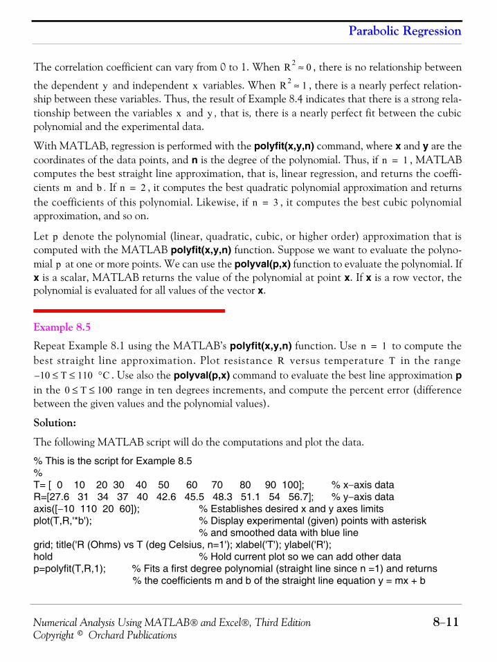
Numerical Analysis Using MATLAB® and Excel®, Third Edition 8−11Copyright © Orchard Publications
Parabolic Regression
The correlation coefficient can vary from 0 to 1. When , there is no relationship between
the dependent and independent variables. When , there is a nearly perfect relation-ship between these variables. Thus, the result of Example 8.4 indicates that there is a strong rela-tionship between the variables and , that is, there is a nearly perfect fit between the cubicpolynomial and the experimental data.
With MATLAB, regression is performed with the polyfit(x,y,n) command, where x and y are thecoordinates of the data points, and n is the degree of the polynomial. Thus, if , MATLABcomputes the best straight line approximation, that is, linear regression, and returns the coeffi-cients and . If , it computes the best quadratic polynomial approximation and returnsthe coefficients of this polynomial. Likewise, if , it computes the best cubic polynomialapproximation, and so on.
Let denote the polynomial (linear, quadratic, cubic, or higher order) approximation that iscomputed with the MATLAB polyfit(x,y,n) function. Suppose we want to evaluate the polyno-mial at one or more points. We can use the polyval(p,x) function to evaluate the polynomial. Ifx is a scalar, MATLAB returns the value of the polynomial at point x. If x is a row vector, thepolynomial is evaluated for all values of the vector x.
Example 8.5
Repeat Example 8.1 using the MATLAB’s polyfit(x,y,n) function. Use to compute thebest straight line approximation. Plot resistance versus temperature in the range
. Use also the polyval(p,x) command to evaluate the best line approximation pin the range in ten degrees increments, and compute the percent error (differencebetween the given values and the polynomial values).
Solution:
The following MATLAB script will do the computations and plot the data.
% This is the script for Example 8.5%T= [ 0 10 20 30 40 50 60 70 80 90 100]; % x−axis dataR=[27.6 31 34 37 40 42.6 45.5 48.3 51.1 54 56.7]; % y−axis dataaxis([−10 110 20 60]); % Establishes desired x and y axes limitsplot(T,R,'*b'); % Display experimental (given) points with asterisk
% and smoothed data with blue linegrid; title('R (Ohms) vs T (deg Celsius, n=1'); xlabel('T'); ylabel('R');hold % Hold current plot so we can add other datap=polyfit(T,R,1); % Fits a first degree polynomial (straight line since n =1) and returns
% the coefficients m and b of the straight line equation y = mx + b
R 2 0≈
y x R 2 1≈
x y
n 1=
m b n 2=
n 3=
p
p
n 1=
R T10– T 110≤ ≤ °C
0 T 100≤ ≤
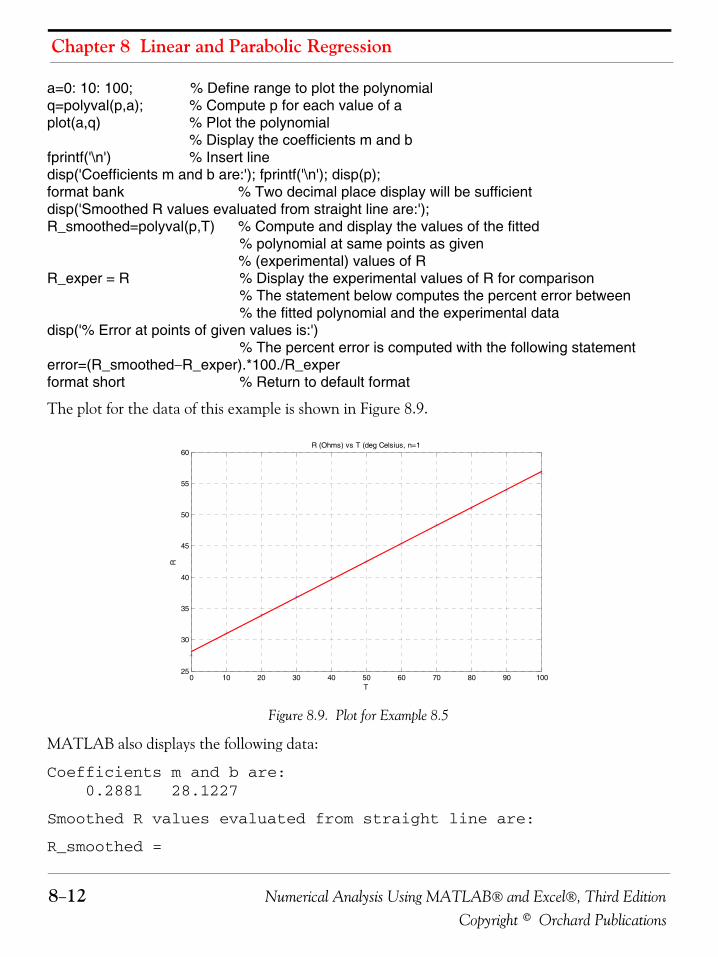
Chapter 8 Linear and Parabolic Regression
8−12 Numerical Analysis Using MATLAB® and Excel®, Third EditionCopyright © Orchard Publications
a=0: 10: 100; % Define range to plot the polynomialq=polyval(p,a); % Compute p for each value of aplot(a,q) % Plot the polynomial
% Display the coefficients m and bfprintf('\n') % Insert linedisp('Coefficients m and b are:'); fprintf('\n'); disp(p);format bank % Two decimal place display will be sufficientdisp('Smoothed R values evaluated from straight line are:'); R_smoothed=polyval(p,T) % Compute and display the values of the fitted
% polynomial at same points as given % (experimental) values of R
R_exper = R % Display the experimental values of R for comparison% The statement below computes the percent error between % the fitted polynomial and the experimental data
disp('% Error at points of given values is:')% The percent error is computed with the following statement
error=(R_smoothed−R_exper).*100./R_experformat short % Return to default format
The plot for the data of this example is shown in Figure 8.9.
Figure 8.9. Plot for Example 8.5
MATLAB also displays the following data:
Coefficients m and b are: 0.2881 28.1227
Smoothed R values evaluated from straight line are:
R_smoothed =
0 10 20 30 40 50 60 70 80 90 10025
30
35
40
45
50
55
60R (Ohms) vs T (deg Celsius, n=1
T
R
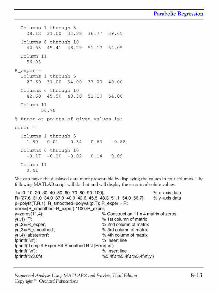
Numerical Analysis Using MATLAB® and Excel®, Third Edition 8−13Copyright © Orchard Publications
Parabolic Regression
Columns 1 through 5 28.12 31.00 33.88 36.77 39.65
Columns 6 through 10 42.53 45.41 48.29 51.17 54.05
Column 11 56.93
R_exper = Columns 1 through 5 27.60 31.00 34.00 37.00 40.00
Columns 6 through 10 42.60 45.50 48.30 51.10 54.00
Column 11 56.70
% Error at points of given values is:
error =
Columns 1 through 5 1.89 0.01 -0.34 -0.63 -0.88
Columns 6 through 10 -0.17 -0.20 -0.02 0.14 0.09
Column 11 0.41
We can make the displayed data more presentable by displaying the values in four columns. Thefollowing MATLAB script will do that and will display the error in absolute values.
T= [0 10 20 30 40 50 60 70 80 90 100]; % x−axis dataR=[27.6 31.0 34.0 37.0 40.0 42.6 45.5 48.3 51.1 54.0 56.7]; % y−axis datap=polyfit(T,R,1); R_smoothed=polyval(p,T); R_exper = R;error=(R_smoothed−R_exper).*100./R_exper;y=zeros(11,4); % Construct an 11 x 4 matrix of zerosy(:,1)=T'; % 1st column of matrixy(:,2)=R_exper'; % 2nd column of matrixy(:,3)=R_smoothed'; % 3rd column of matrixy(:,4)=abs(error)'; % 4th column of matrixfprintf(' \n'); % Insert linefprintf('Temp \t Exper R\t Smoothed R \t |Error| \n')fprintf(' \n'); % Insert linefprintf('%3.0f\t %5.4f\t %5.4f\t %5.4f\n',y')
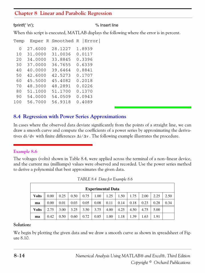
Chapter 8 Linear and Parabolic Regression
8−14 Numerical Analysis Using MATLAB® and Excel®, Third EditionCopyright © Orchard Publications
fprintf(' \n'); % Insert line
When this script is executed, MATLAB displays the following where the error is in percent.
Temp Exper R Smoothed R |Error|
0 27.6000 28.1227 1.8939 10 31.0000 31.0036 0.0117 20 34.0000 33.8845 0.3396 30 37.0000 36.7655 0.6339 40 40.0000 39.6464 0.8841 50 42.6000 42.5273 0.1707 60 45.5000 45.4082 0.2018 70 48.3000 48.2891 0.0226 80 51.1000 51.1700 0.1370 90 54.0000 54.0509 0.0943100 56.7000 56.9318 0.4089
8.4 Regression with Power Series ApproximationsIn cases where the observed data deviate significantly from the points of a straight line, we candraw a smooth curve and compute the coefficients of a power series by approximating the deriva-tives with finite differences . The following example illustrates the procedure.
Example 8.6 The voltages (volts) shown in Table 8.4, were applied across the terminal of a non−linear device,and the current ma (milliamps) values were observed and recorded. Use the power series methodto derive a polynomial that best approximates the given data.
Solution:
We begin by plotting the given data and we draw a smooth curve as shown in spreadsheet of Fig-ure 8.10.
TABLE 8.4 Data for Example 8.6
Experimental Data
Volts 0.00 0.25 0.50 0.75 1.00 1.25 1.50 1.75 2.00 2.25 2.50
ma 0.00 0.01 0.03 0.05 0.08 0.11 0.14 0.18 0.23 0.28 0.34
Volts 2.75 3.00 3.25 3.50 3.75 4.00 4.25 4.50 4.75 5.00
ma 0.42 0.50 0.60 0.72 0.85 1.00 1.18 1.39 1.63 1.91
di dv⁄ Δi Δv⁄
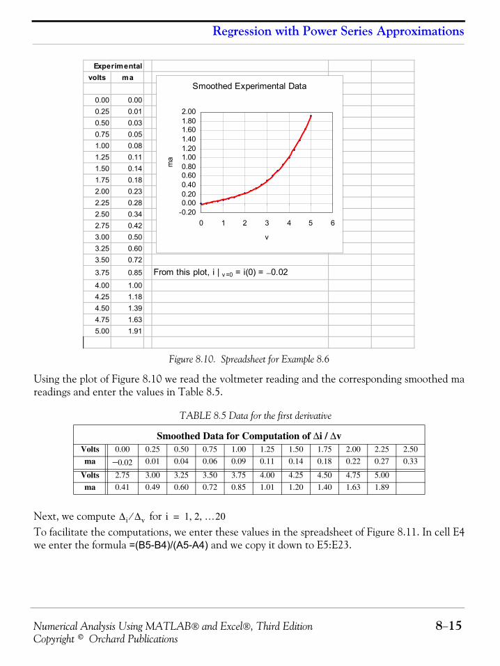
Numerical Analysis Using MATLAB® and Excel®, Third Edition 8−15Copyright © Orchard Publications
Regression with Power Series Approximations
Figure 8.10. Spreadsheet for Example 8.6
Using the plot of Figure 8.10 we read the voltmeter reading and the corresponding smoothed mareadings and enter the values in Table 8.5.
Next, we compute for To facilitate the computations, we enter these values in the spreadsheet of Figure 8.11. In cell E4we enter the formula =(B5-B4)/(A5-A4) and we copy it down to E5:E23.
TABLE 8.5 Data for the first derivative
Smoothed Data for Computation of Δi / ΔvVolts 0.00 0.25 0.50 0.75 1.00 1.25 1.50 1.75 2.00 2.25 2.50
ma −0.02 0.01 0.04 0.06 0.09 0.11 0.14 0.18 0.22 0.27 0.33
Volts 2.75 3.00 3.25 3.50 3.75 4.00 4.25 4.50 4.75 5.00
ma 0.41 0.49 0.60 0.72 0.85 1.01 1.20 1.40 1.63 1.89
Experimentalvolts ma
0.00 0.000.25 0.010.50 0.030.75 0.051.00 0.081.25 0.111.50 0.141.75 0.182.00 0.232.25 0.282.50 0.342.75 0.423.00 0.503.25 0.603.50 0.72
3.75 0.85 From this plot, i | v =0 = i(0) = −0.024.00 1.004.25 1.184.50 1.394.75 1.635.00 1.91
Smoothed Experimental Data
-0.200.000.200.400.600.801.001.201.401.601.802.00
0 1 2 3 4 5 6
v
ma
Δi Δv⁄ i 1 2 …20, ,=
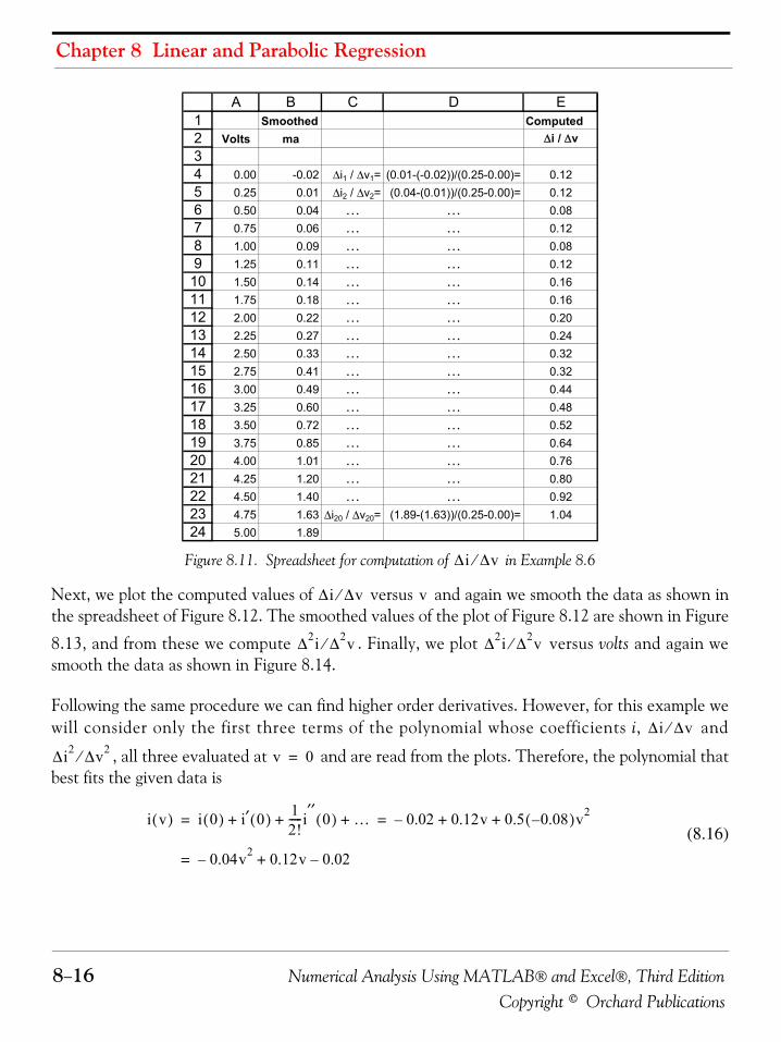
Chapter 8 Linear and Parabolic Regression
8−16 Numerical Analysis Using MATLAB® and Excel®, Third EditionCopyright © Orchard Publications
Figure 8.11. Spreadsheet for computation of in Example 8.6
Next, we plot the computed values of versus and again we smooth the data as shown inthe spreadsheet of Figure 8.12. The smoothed values of the plot of Figure 8.12 are shown in Figure
8.13, and from these we compute . Finally, we plot versus volts and again wesmooth the data as shown in Figure 8.14.
Following the same procedure we can find higher order derivatives. However, for this example wewill consider only the first three terms of the polynomial whose coefficients i, and
, all three evaluated at and are read from the plots. Therefore, the polynomial thatbest fits the given data is
(8.16)
123456789101112131415161718192021222324
A B C D ESmoothed Computed
Volts ma Δi / Δv
0.00 -0.02 Δi1 / Δv1= (0.01-(-0.02))/(0.25-0.00)= 0.120.25 0.01 Δi2 / Δv2= (0.04-(0.01))/(0.25-0.00)= 0.120.50 0.04 … … 0.080.75 0.06 … … 0.121.00 0.09 … … 0.081.25 0.11 … … 0.121.50 0.14 … … 0.161.75 0.18 … … 0.162.00 0.22 … … 0.202.25 0.27 … … 0.242.50 0.33 … … 0.322.75 0.41 … … 0.323.00 0.49 … … 0.443.25 0.60 … … 0.483.50 0.72 … … 0.523.75 0.85 … … 0.644.00 1.01 … … 0.764.25 1.20 … … 0.804.50 1.40 … … 0.924.75 1.63 Δi20 / Δv20= (1.89-(1.63))/(0.25-0.00)= 1.045.00 1.89
Δi Δv⁄
Δi Δv⁄ v
Δ2i Δ2v⁄ Δ2i Δ2v⁄
Δi Δv⁄
Δi2 Δv2⁄ v 0=
i v( ) i 0( ) i ′ 0( ) 12!-----i ′′ 0( ) …+ + + 0.02– 0.12v 0.5 0.08–( )v2+ += =
0.04v2– 0.12v 0.02–+=
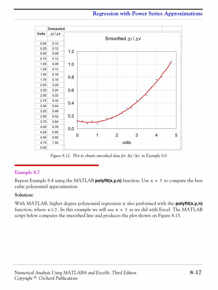
Numerical Analysis Using MATLAB® and Excel®, Third Edition 8−17Copyright © Orchard Publications
Regression with Power Series Approximations
Figure 8.12. Plot to obtain smoothed data for in Example 8.6
Example 8.7
Repeat Example 8.4 using the MATLAB polyfit(x,y,n) function. Use to compute the bestcubic polynomial approximation.
Solution:
With MATLAB, higher degree polynomial regression is also performed with the polyfit(x,y,n)function, where . In this example we will use as we did with Excel. The MATLABscript below computes the smoothed line and produces the plot shown on Figure 8.15.
ComputedVolts Δ i / Δv Δ i / Δv
0.00 0.12 -0.020.25 0.12 0.010.50 0.08 0.040.75 0.12 0.061.00 0.08 0.091.25 0.12 0.111.50 0.16 0.141.75 0.16 0.182.00 0.20 0.222.25 0.24 0.272.50 0.32 0.332.75 0.32 0.413.00 0.44 0.493.25 0.48 From this plot, (Δi / Δv) | v=0 = i'(0) = 0.12 0.603.50 0.52 0.723.75 0.64 0.854.00 0.76 1.014.25 0.80 1.204.50 0.92 1.404.75 1.04 1.635.00 1.89
Smoothed Δ i / Δv
0.0
0.2
0.4
0.6
0.8
1.0
1.2
0 1 2 3 4 5
volts
Δi Δv⁄
n 3=
n 2≥ n 3=
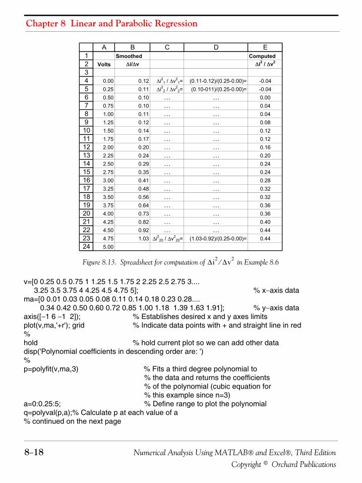
Chapter 8 Linear and Parabolic Regression
8−18 Numerical Analysis Using MATLAB® and Excel®, Third EditionCopyright © Orchard Publications
Figure 8.13. Spreadsheet for computation of in Example 8.6
v=[0 0.25 0.5 0.75 1 1.25 1.5 1.75 2 2.25 2.5 2.75 3.... 3.25 3.5 3.75 4 4.25 4.5 4.75 5]; % x−axis datama=[0 0.01 0.03 0.05 0.08 0.11 0.14 0.18 0.23 0.28.... 0.34 0.42 0.50 0.60 0.72 0.85 1.00 1.18 1.39 1.63 1.91]; % y−axis dataaxis([−1 6 −1 2]); % Establishes desired x and y axes limitsplot(v,ma,'+r'); grid % Indicate data points with + and straight line in red %hold % hold current plot so we can add other datadisp('Polynomial coefficients in descending order are: ')%p=polyfit(v,ma,3) % Fits a third degree polynomial to
% the data and returns the coefficients% of the polynomial (cubic equation for% this example since n=3)
a=0:0.25:5; % Define range to plot the polynomialq=polyval(p,a);% Calculate p at each value of a% continued on the next page
123456789101112131415161718192021222324
A B C D ESmoothed Computed
Volts Δi/Δv Δi2 / Δv2
0.00 0.12 Δi21 / Δv21= (0.11-0.12)/(0.25-0.00)= -0.04
0.25 0.11 Δi22 / Δv22= (0.10-011)/(0.25-0.00)= -0.04
0.50 0.10 … … 0.000.75 0.10 … … 0.041.00 0.11 … … 0.041.25 0.12 … … 0.081.50 0.14 … … 0.121.75 0.17 … … 0.122.00 0.20 … … 0.162.25 0.24 … … 0.202.50 0.29 … … 0.242.75 0.35 … … 0.243.00 0.41 … … 0.283.25 0.48 … … 0.323.50 0.56 … … 0.323.75 0.64 … … 0.364.00 0.73 … … 0.364.25 0.82 … … 0.404.50 0.92 … … 0.444.75 1.03 Δi220 / Δv2
20= (1.03-0.92)/(0.25-0.00)= 0.445.00
Δi2 Δv2⁄
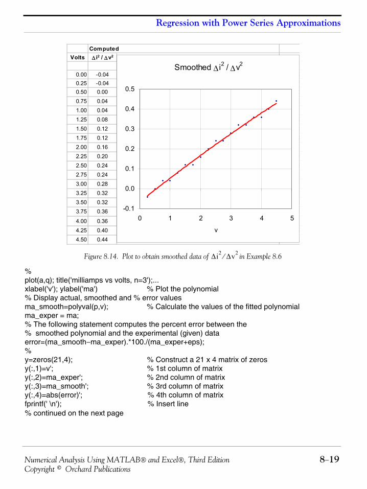
Numerical Analysis Using MATLAB® and Excel®, Third Edition 8−19Copyright © Orchard Publications
Regression with Power Series Approximations
Figure 8.14. Plot to obtain smoothed data of in Example 8.6
% plot(a,q); title('milliamps vs volts, n=3');...xlabel('v'); ylabel('ma') % Plot the polynomial% Display actual, smoothed and % error valuesma_smooth=polyval(p,v); % Calculate the values of the fitted polynomialma_exper = ma;% The following statement computes the percent error between the % smoothed polynomial and the experimental (given) dataerror=(ma_smooth−ma_exper).*100./(ma_exper+eps);%y=zeros(21,4); % Construct a 21 x 4 matrix of zerosy(:,1)=v'; % 1st column of matrixy(:,2)=ma_exper'; % 2nd column of matrixy(:,3)=ma_smooth'; % 3rd column of matrixy(:,4)=abs(error)'; % 4th column of matrixfprintf(' \n'); % Insert line% continued on the next page
ComputedVolts Δ i2 / Δv2
0.00 -0.04 0.120.25 -0.04 0.110.50 0.00 0.100.75 0.04 0.101.00 0.04 0.111.25 0.08 0.121.50 0.12 0.141.75 0.12 0.172.00 0.16 0.202.25 0.20 0.242.50 0.24 0.292.75 0.24 0.353.00 0.28 0.413.25 0.32 0.483.50 0.32 0.563.75 0.36 0.64
4.00 0.36 From this plot, (Δi2 / Δv2) | v=0 = i''(0) = −0.08 0.734.25 0.40 0.824.50 0.44 0.92
Smoothed Δ i2 / Δv2
-0.1
0.0
0.1
0.2
0.3
0.4
0.5
0 1 2 3 4 5
v
Δi2 Δv2⁄
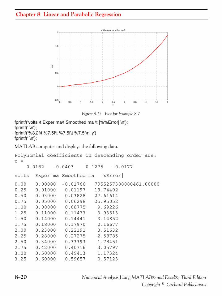
Chapter 8 Linear and Parabolic Regression
8−20 Numerical Analysis Using MATLAB® and Excel®, Third EditionCopyright © Orchard Publications
Figure 8.15. Plot for Example 8.7
fprintf('volts \t Exper ma\t Smoothed ma \t |%%Error| \n'); fprintf(' \n');fprintf('%3.2f\t %7.5f\t %7.5f\t %7.5f\n',y')fprintf(' \n');
MATLAB computes and displays the following data.
Polynomial coefficients in descending order are: p = 0.0182 -0.0403 0.1275 -0.0177
volts Exper ma Smoothed ma |%Error| 0.00 0.00000 -0.01766 7955257388080461.000000.25 0.01000 0.01197 19.744020.50 0.03000 0.03828 27.616140.75 0.05000 0.06298 25.950521.00 0.08000 0.08775 9.692261.25 0.11000 0.11433 3.935131.50 0.14000 0.14441 3.148521.75 0.18000 0.17970 0.166772.00 0.23000 0.22191 3.516322.25 0.28000 0.27275 2.587852.50 0.34000 0.33393 1.784512.75 0.42000 0.40716 3.057973.00 0.50000 0.49413 1.173243.25 0.60000 0.59657 0.57123
0 0.5 1 1.5 2 2.5 3 3.5 4 4.5 5-0.5
0
0.5
1
1.5
2milliamps vs volts, n=3
v
ma
Numerical Analysis Using MATLAB® and Excel®, Third Edition 8−21Copyright © Orchard Publications
Regression with Power Series Approximations
3.50 0.72000 0.71618 0.530403.75 0.85000 0.85467 0.549114.00 1.00000 1.01374 1.373994.25 1.18000 1.19511 1.280204.50 1.39000 1.40048 0.753624.75 1.63000 1.63155 0.095385.00 1.91000 1.89005 1.04436
We will conclude this chapter with one more example to illustrate the uses of the MATLABpolyfit(x,y,n) and polyval(p,x) functions.
Example 8.8 Use MATLAB to
a. plot the function(8.17)
in the interval radians.
b. compute
c. plot versus for these values and use the MATLAB polyfit(x,y,n) and polyval(p,x) func-tions to find a suitable polynomial that best fits the and data.
Solution:
a. The fplot function below plots . We added eps to avoid division by zero.
fplot('sin(x)./(x+eps)',[0 16 −0.5 1]); grid;...title('(sinx)/x curve for x > 0')
The plot for the function of (8.17) is shown in Figure 8.16.
b. We use the script below to evaluate at the specified points.
x=0:2:16; y=sin(x)./(x+eps)p7=polyfit(x,y,7); % of x and y with fifth, seventh,p9=polyfit(x,y,9); % and ninth degree polynomials% continued on the next page
y xsin x⁄=
0 x 16≤ ≤
y 0( ) y 2( ) y 4( ) y 6( ) y 8( ) y 10( ) y 12( ) y 14( ) y 16( ), , , , , , , ,
y xx y
y xsin x⁄=
y
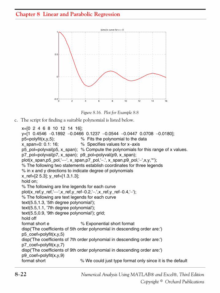
Chapter 8 Linear and Parabolic Regression
8−22 Numerical Analysis Using MATLAB® and Excel®, Third EditionCopyright © Orchard Publications
Figure 8.16. Plot for Example 8.8
c. The script for finding a suitable polynomial is listed below.
x=[0 2 4 6 8 10 12 14 16];y=[1 0.4546 −0.1892 −0.0466 0.1237 −0.0544 −0.0447 0.0708 −0.0180];p5=polyfit(x,y,5); % Fits the polynomial to the datax_span=0: 0.1: 16; % Specifies values for x−axisp5_pol=polyval(p5, x_span); % Compute the polynomials for this range of x values.p7_pol=polyval(p7, x_span); p9_pol=polyval(p9, x_span);plot(x_span,p5_pol,'−−', x_span,p7_pol,'−.', x_span,p9_pol,'−',x,y,'*');% The following two statements establish coordinates for three legends% in x and y directions to indicate degree of polynomialsx_ref=[2 5.3]; y_ref=[1.3,1.3];hold on;% The following are line legends for each curveplot(x_ref,y_ref,'−−',x_ref,y_ref−0.2,'−.',x_ref,y_ref−0.4,'−'); % The following are text legends for each curvetext(5.5,1.3, '5th degree polynomial');text(5.5,1.1, '7th degree polynomial');text(5.5,0.9, '9th degree polynomial'); grid;hold offformat short e % Exponential short formatdisp('The coefficients of 5th order polynomial in descending order are:')p5_coef=polyfit(x,y,5)disp('The coefficients of 7th order polynomial in descending order are:')p7_coef=polyfit(x,y,7)disp('The coefficients of 9th order polynomial in descending order are:')p9_coef=polyfit(x,y,9)format short % We could just type format only since it is the default
0 2 4 6 8 10 12 14 16-0.5
0
0.5
1(sinx)/x curve for x > 0
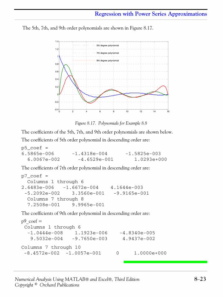
Numerical Analysis Using MATLAB® and Excel®, Third Edition 8−23Copyright © Orchard Publications
Regression with Power Series Approximations
The 5th, 7th, and 9th order polynomials are shown in Figure 8.17.
Figure 8.17. Polynomials for Example 8.8
The coefficients of the 5th, 7th, and 9th order polynomials are shown below.
The coefficients of 5th order polynomial in descending order are:
p5_coef = 6.5865e-006 -1.4318e-004 -1.5825e-003
6.0067e-002 -4.6529e-001 1.0293e+000
The coefficients of 7th order polynomial in descending order are:
p7_coef = Columns 1 through 6
2.6483e-006 -1.6672e-004 4.1644e-003 -5.2092e-002 3.3560e-001 -9.9165e-001 Columns 7 through 8 7.2508e-001 9.9965e-001
The coefficients of 9th order polynomial in descending order are:
p9_coef = Columns 1 through 6
-1.0444e-008 1.1923e-006 -4.8340e-005 9.5032e-004 -9.7650e-003 4.9437e-002
Columns 7 through 10 -8.4572e-002 -1.0057e-001 0 1.0000e+000
0 2 4 6 8 10 12 14 16-0.4
-0.2
0
0.2
0.4
0.6
0.8
1
1.2
1.4
5th degree polynomial
7th degree polynomial
9th degree polynomial
Chapter 8 Linear and Parabolic Regression
8−24 Numerical Analysis Using MATLAB® and Excel®, Third EditionCopyright © Orchard Publications
8.5 Summary• Curve fitting is the process of finding equations to approximate straight lines and curves that
best fit given sets of data.
• Regression is the process of finding the dependent variable from some data of the independentvariable . Regression can be linear (straight line) or curved (quadratic, cubic, etc.)
• The best fitting straight line or curve has the property that and itis referred to as the least−squares curve. A straight line that satisfies this property is called a leastsquares line. If it is a parabola, we call it a least−squares parabola.
• We perform linear regression with the method of least squares. With this method, we computethe coefficients (slope) and (y-intercept) of the straight line equation suchthat the sum of the squares of the errors will be minimum. The values of and can be foundfrom the relations
where
,
,
The values of and are computed from
where
• We find the least−squares parabola that fits a set of sample points with wherethe coefficients are found from
where = number of data points.
yx
d12 d2
2 … d32+ + + minimum=
m b y mx b+=m b
Σx2( )m Σx( )b+ Σxy=
Σx( )m nb+ Σy=
Σx sum of the numbers x= Σy sum of the numbers y=
Σxy sum of the numbers of the product xy= Σx2 sum of the numbers x squared=
n number of data x=
m b
mD1Δ
------= bD2Δ
------=
Δ Σx2 ΣxΣx n
= D1Σxy ΣxΣy n
= D2Σx2 ΣxyΣx Σy
=
y ax2 b c+ +=
a b and c, ,
Σx2( )a Σx( )b nc+ + Σy=
Σx3( )a Σx2( )b Σx( )c+ + Σxy=
Σx4( )a Σx3( )b Σx2( )c+ + Σx2y=
n
Numerical Analysis Using MATLAB® and Excel®, Third Edition 8−25Copyright © Orchard Publications
Summary
• With MATLAB, regression is performed with the polyfit(x,y,n) command, where x and y arethe coordinates of the data points, and n is the degree of the polynomial. Thus, if ,MATLAB computes the best straight line approximation, that is, linear regression, and returnsthe coefficients and . If , it computes the best quadratic polynomial approximationand returns the coefficients of this polynomial. Likewise, if , it computes the best cubicpolynomial approximation, and so on.
• In cases where the observed data deviate significantly from the points of a straight line, we candraw a smooth curve and compute the coefficients of a power series by approximating thederivatives with finite differences .
n 1=
m b n 2=
n 3=
dy dx⁄ Δy Δx⁄
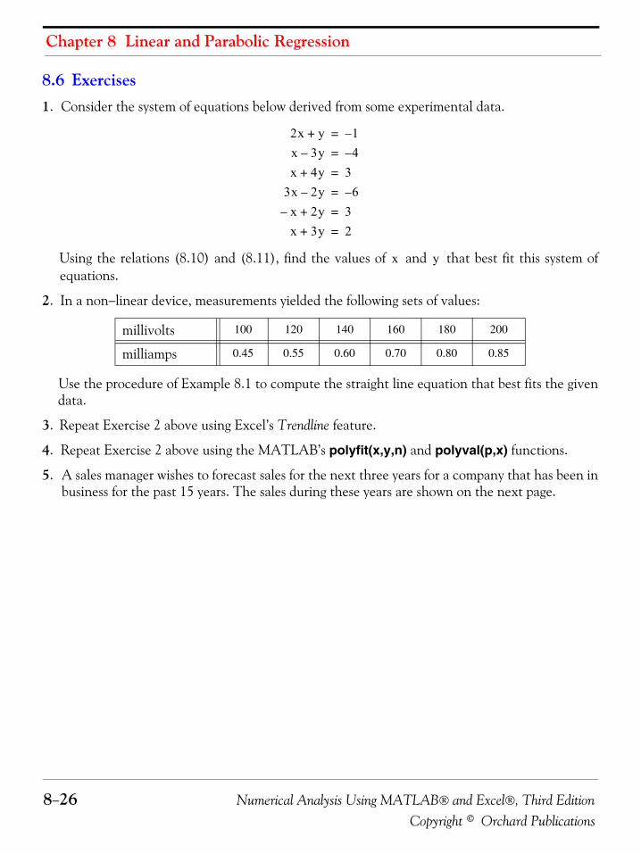
Chapter 8 Linear and Parabolic Regression
8−26 Numerical Analysis Using MATLAB® and Excel®, Third EditionCopyright © Orchard Publications
8.6 Exercises1. Consider the system of equations below derived from some experimental data.
Using the relations (8.10) and (8.11), find the values of and that best fit this system ofequations.
2. In a non−linear device, measurements yielded the following sets of values:
Use the procedure of Example 8.1 to compute the straight line equation that best fits the givendata.
3. Repeat Exercise 2 above using Excel’s Trendline feature.
4. Repeat Exercise 2 above using the MATLAB’s polyfit(x,y,n) and polyval(p,x) functions.
5. A sales manager wishes to forecast sales for the next three years for a company that has been inbusiness for the past 15 years. The sales during these years are shown on the next page.
millivolts 100 120 140 160 180 200
milliamps 0.45 0.55 0.60 0.70 0.80 0.85
2x y+ 1–=
x 3y– 4–=
x 4y+ 3=
3x 2y– 6–=
x– 2y+ 3=
x 3y+ 2=
x y
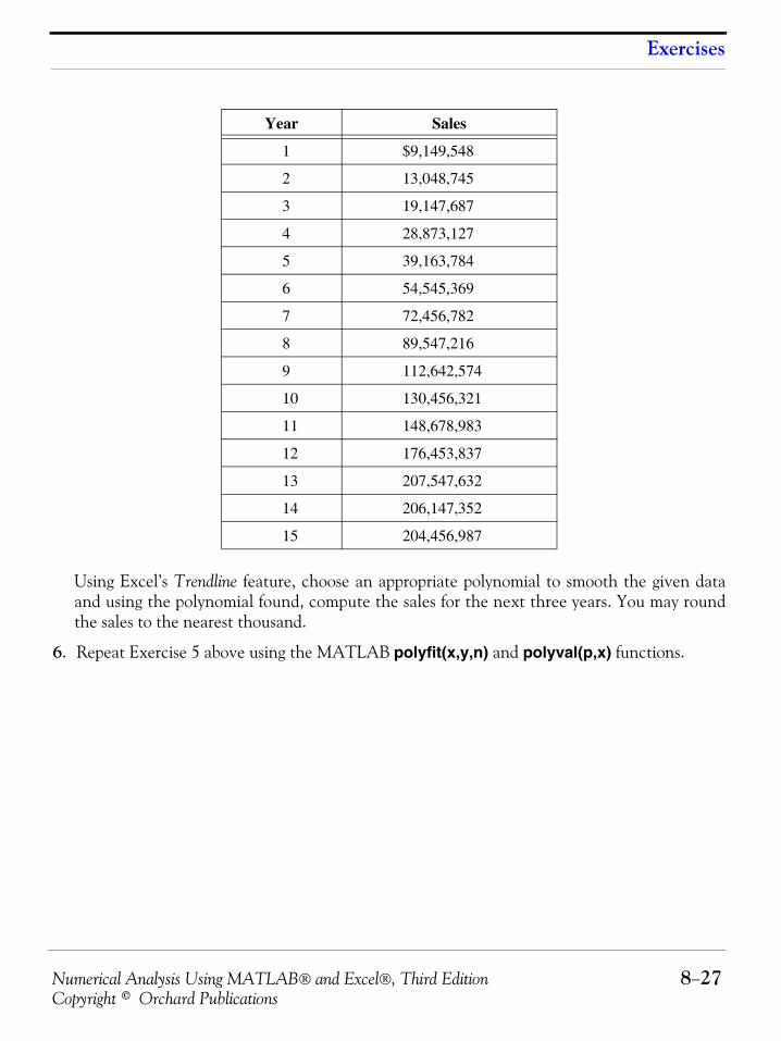
Numerical Analysis Using MATLAB® and Excel®, Third Edition 8−27Copyright © Orchard Publications
Exercises
Using Excel’s Trendline feature, choose an appropriate polynomial to smooth the given dataand using the polynomial found, compute the sales for the next three years. You may roundthe sales to the nearest thousand.
6. Repeat Exercise 5 above using the MATLAB polyfit(x,y,n) and polyval(p,x) functions.
Year Sales
1 $9,149,548
2 13,048,745
3 19,147,687
4 28,873,127
5 39,163,784
6 54,545,369
7 72,456,782
8 89,547,216
9 112,642,574
10 130,456,321
11 148,678,983
12 176,453,837
13 207,547,632
14 206,147,352
15 204,456,987
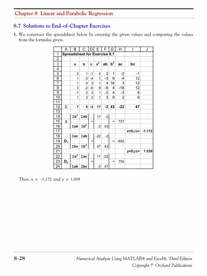
Chapter 8 Linear and Parabolic Regression
8−28 Numerical Analysis Using MATLAB® and Excel®, Third EditionCopyright © Orchard Publications
8.7 Solutions to End−of−Chapter Exercises1. We construct the spreadsheet below by entering the given values and computing the values
from the formulas given.
Thus, and
123456789101112131415161718192021222324
A B C D E F G H I JSpreadsheet for Exercise 8.1
a b c a2 ab b2 ac bc
2 1 -1 4 2 1 -2 -11 -3 -4 1 -3 9 -4 121 4 3 1 4 16 3 123 -2 -6 9 -6 4 -18 12
-1 2 3 1 -2 4 -3 61 3 2 1 3 9 2 6
Σ 7 5 -3 17 -2 43 -22 47
Σa2 Σab 17 -2Δ = = 727
Σab Σb2 -2 43x=D1/Δ= -1.172
Σac Σab -22 -2D1 = = -852
Σbc Σb2 47 43y=D2/Δ= 1.039
Σa2 Σac 17 -22D2 = = 755
Σab Σbc -2 47
x 1.172–= y 1.039=
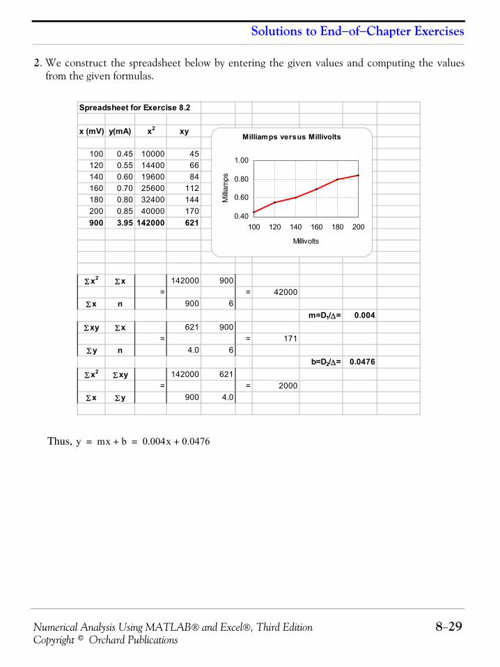
Numerical Analysis Using MATLAB® and Excel®, Third Edition 8−29Copyright © Orchard Publications
Solutions to End−of−Chapter Exercises
2. We construct the spreadsheet below by entering the given values and computing the valuesfrom the given formulas.
Thus,
Spreadsheet for Exercise 8.2
x (mV) y(mA) x2 xy
100 0.45 10000 45120 0.55 14400 66140 0.60 19600 84160 0.70 25600 112180 0.80 32400 144200 0.85 40000 170900 3.95 142000 621
Σ x2 Σ x 142000 900= = 42000
Σ x n 900 6m=D1/Δ= 0.004
Σ xy Σ x 621 900= = 171
Σ y n 4.0 6b=D2/Δ= 0.0476
Σ x2 Σ xy 142000 621= = 2000
Σ x Σ y 900 4.0
Milliamps versus Millivolts
0.40
0.60
0.80
1.00
100 120 140 160 180 200
Millivolts
Milli
amps
y mx b+ 0.004x 0.0476+= =
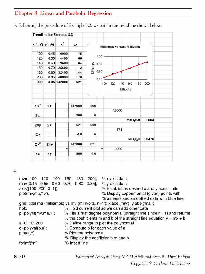
Chapter 8 Linear and Parabolic Regression
8−30 Numerical Analysis Using MATLAB® and Excel®, Third EditionCopyright © Orchard Publications
3. Following the procedure of Example 8.2, we obtain the trendline shown below.
4.
mv= [100 120 140 160 180 200]; % x-axis datama=[0.45 0.55 0.60 0.70 0.80 0.85]; % y-axis dataaxis([100 200 0 1]); % Establishes desired x and y axes limitsplot(mv,ma,'*b'); % Display experimental (given) points with
% asterisk and smoothed data with blue linegrid; title('ma (milliamps) vs mv (millivolts, n=1'); xlabel('mv'); ylabel('ma');hold % Hold current plot so we can add other datap=polyfit(mv,ma,1); % Fits a first degree polynomial (straight line since n =1) and returns
% the coefficients m and b of the straight line equation y = mx + ba=0: 10: 200; % Define range to plot the polynomialq=polyval(p,a); % Compute p for each value of aplot(a,q) % Plot the polynomial
% Display the coefficients m and bfprintf('\n') % Insert line
Trendline for Exercise 8.3
x (mV) y(mA) x2 xy
100 0.45 10000 45120 0.55 14400 66140 0.60 19600 84160 0.70 25600 112180 0.80 32400 144200 0.85 40000 170900 3.95 142000 621
Σ x2 Σ x 142000 900= = 42000
Σ x n 900 6m=D1/Δ= 0.004
Σ xy Σ x 621 900= = 171
Σ y n 4.0 6b=D2/Δ= 0.0476
Σ x2 Σ xy 142000 621= = 2000
Σ x Σ y 900 4.0
Milliamps versus Millivolts
0.40
0.60
0.80
1.00
100 120 140 160 180 200
MillivoltsM
illiam
ps
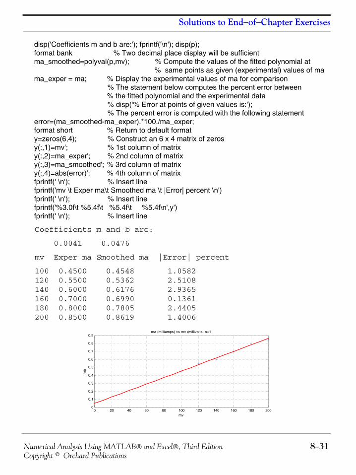
Numerical Analysis Using MATLAB® and Excel®, Third Edition 8−31Copyright © Orchard Publications
Solutions to End−of−Chapter Exercises
disp('Coefficients m and b are:'); fprintf('\n'); disp(p);format bank % Two decimal place display will be sufficientma_smoothed=polyval(p,mv); % Compute the values of the fitted polynomial at
% same points as given (experimental) values of mama_exper = ma; % Display the experimental values of ma for comparison
% The statement below computes the percent error between % the fitted polynomial and the experimental data% disp('% Error at points of given values is:');% The percent error is computed with the following statement
error=(ma_smoothed-ma_exper).*100./ma_exper;format short % Return to default formaty=zeros(6,4); % Construct an 6 x 4 matrix of zerosy(:,1)=mv'; % 1st column of matrixy(:,2)=ma_exper'; % 2nd column of matrixy(:,3)=ma_smoothed'; % 3rd column of matrixy(:,4)=abs(error)'; % 4th column of matrixfprintf(' \n'); % Insert linefprintf('mv \t Exper ma\t Smoothed ma \t |Error| percent \n')fprintf(' \n'); % Insert linefprintf('%3.0f\t %5.4f\t %5.4f\t %5.4f\n',y')fprintf(' \n'); % Insert line
Coefficients m and b are:
0.0041 0.0476
mv Exper ma Smoothed ma |Error| percent
100 0.4500 0.4548 1.0582120 0.5500 0.5362 2.5108140 0.6000 0.6176 2.9365160 0.7000 0.6990 0.1361180 0.8000 0.7805 2.4405200 0.8500 0.8619 1.4006
0 20 40 60 80 100 120 140 160 180 2000
0.1
0.2
0.3
0.4
0.5
0.6
0.7
0.8
0.9ma (milliamps) vs mv (millivolts, n=1
mv
ma
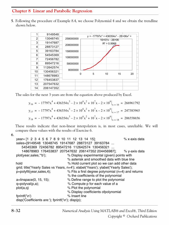
Chapter 8 Linear and Parabolic Regression
8−32 Numerical Analysis Using MATLAB® and Excel®, Third EditionCopyright © Orchard Publications
5. Following the procedure of Example 8.4, we choose Polynomial 4 and we obtain the trendlineshown below.
The sales for the next 3 years are from the equation above produced by Excel.
These results indicate that non-linear interpolation is, in most cases, unreliable. We willcompare these values with the results of Exercise 6.
6.year= [1 2 3 4 5 6 7 8 9 10 11 12 13 14 15]; % x-axis datasales=[9149548 13048745 19147687 28873127 39163784 ...
54545369 72456782 89547216 112642574 130456321 ... 148678983 176453837 207547632 206147352 204456987]; % y-axis data
plot(year,sales,'*b'); % Display experimental (given) points with% asterisk and smoothed data with blue line
hold % Hold current plot so we can add other datagrid; title('Yearly Sales vs Years, n=4'); xlabel('Years'); ylabel('Yearly Sales');p=polyfit(year,sales,4); % Fits a first degree polynomial (n=4) and returns
% the coefficients of the polynomiala=linspace(0, 15, 15); % Define range to plot the polynomialq=polyval(p,a); % Compute p for each value of aplot(a,q) % Plot the polynomial
% Display coefficients ofpolynomialfprintf('\n') % Insert linedisp('Coefficients are:'); fprintf('\n'); disp(p);
1 91495482 130487453 191476874 288731275 391637846 545453697 724567828 895472169 112642574
10 13045632111 14867898312 17645383713 20754763214 206147352
y = -17797x4 + 436354x3 - 2E+06x2 + 1E+07x - 2E+06
R2 = 0.9966
8000000
58000000
108000000
158000000
208000000
258000000
0 5 10 15 20
y16 17797x4– 436354x3 2 106x2×– 107x 2 106×–+ + x 16=266961792= =
y17 17797x4– 436354x3 2 106x2×– 107x 2 106×–+ + x 17=247383965= =
y18 17797x4– 436354x3 2 106x2×– 107x 2 106×–+ + x 18=206558656= =
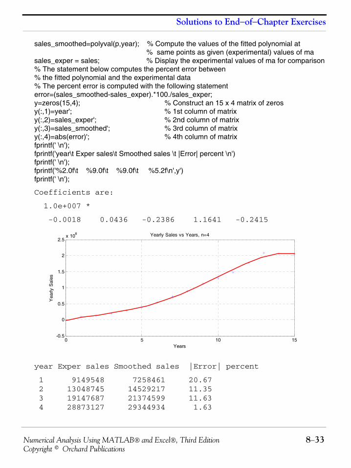
Numerical Analysis Using MATLAB® and Excel®, Third Edition 8−33Copyright © Orchard Publications
Solutions to End−of−Chapter Exercises
sales_smoothed=polyval(p,year); % Compute the values of the fitted polynomial at% same points as given (experimental) values of ma
sales_exper = sales; % Display the experimental values of ma for comparison% The statement below computes the percent error between % the fitted polynomial and the experimental data% The percent error is computed with the following statementerror=(sales_smoothed-sales_exper).*100./sales_exper;y=zeros(15,4); % Construct an 15 x 4 matrix of zerosy(:,1)=year'; % 1st column of matrixy(:,2)=sales_exper'; % 2nd column of matrixy(:,3)=sales_smoothed'; % 3rd column of matrixy(:,4)=abs(error)'; % 4th column of matrixfprintf(' \n');fprintf('year\t Exper sales\t Smoothed sales \t |Error| percent \n')fprintf(' \n');fprintf('%2.0f\t %9.0f\t %9.0f\t %5.2f\n',y')fprintf(' \n');
Coefficients are:
1.0e+007 *
-0.0018 0.0436 -0.2386 1.1641 -0.2415
year Exper sales Smoothed sales |Error| percent
1 9149548 7258461 20.67 2 13048745 14529217 11.35 3 19147687 21374599 11.63 4 28873127 29344934 1.63
0 5 10 15-0.5
0
0.5
1
1.5
2
2.5x 10⁸ Yearly Sales vs Years, n=4
Years
Yea
rly S
ales
Chapter 8 Linear and Parabolic Regression
8−34 Numerical Analysis Using MATLAB® and Excel®, Third EditionCopyright © Orchard Publications
5 39163784 39563426 1.02 6 54545369 52726163 3.34 7 72456782 69102111 4.63 8 89547216 88533118 1.13 9 112642574 110433913 1.9610 130456321 133792104 2.5611 148678983 157168183 5.7112 176453837 178695519 1.2713 207547632 196080363 5.5314 206147352 206601848 0.2215 204456987 207111986 1.30
From the coefficients produced by MATLAB, shown on the previous page, we form the poly-nomial
and from it we find the values of (the yearly sales) as follows:
x=16; y16=−1.8*10^4*x^4+4.36*10^5*x^3−2.386*10^6*x^2+1.1641*10^7*x−2.415*10^6;x=17; y17=−1.8*10^4*x^4+4.36*10^5*x^3−2.386*10^6*x^2+1.1641*10^7*x−2.415*10^6;x=18; y18=−1.8*10^4*x^4+4.36*10^5*x^3−2.386*10^6*x^2+1.1641*10^7*x−2.415*10^6;
y16, y17, y18
y16 =
1.7923e+008
y17 =
1.4462e+008
y18 =
8.7243e+007
These values vary significantly from those of Exercise 5. As stated above, non-linear interpola-tion especially for polynomials of fourth degree and higher give inaccurate results. We shouldremember that the equations produced by both Excel and MATLAB represent the equationsthat best fit the experimental values. For extrapolation, linear regression gives the best approx-imations.
y 1.8 104x4×– 4.36 105x3× 2.386 106× x2– 1.1641 107x 2.415 106×–×+ +=
y
Numerical Analysis Using MATLAB® and Excel®, Third Edition 9−1Copyright © Orchard Publications
Chapter 9
Solution of Differential Equations by Numerical Methods
his chapter is an introduction to several methods that can be used to obtain approximatesolutions of differential equations. Such approximations are necessary when no exact solu-tion can be found. The Taylor, Runge−Kutta, Adams’, and Milne’s methods are discussed.
9.1 Taylor Series Method
We recall from Chapter 6 that the Taylor series expansion about point is
(9.1)
Now, if is a value close to , we can find the approximate value of by using thefirst terms in the Taylor expansion of about . Letting in (9.1), weobtain:
(9.2)
Obviously, to minimize the error we need to keep sufficiently small.
For another value , close to , we repeat the procedure with ; then,
(9.3)
In general,
(9.4)
Example 9.1 Use the Taylor series method to obtain a solution of
(9.5)
correct to four decimal places for values , , , , , and with the initial condition .
Ta
yn f x( )= f a( ) f' a( ) x a–( ) f'' a( )2!
------------ x a–( )2 … f n( ) a( )n!
----------------- x a–( )n+ + + +=
x1 a> a y1 f x1( )
k 1+ f x1( ) x a= h1 x a–=
y1 y0 y'0h112!-----y''0h1
2 13!-----y'''0h1
3 14!-----y0
4( )h14 …+ + + + +=
f x1( ) y1– h1
x2 x1> x1 h2 x2 x1–=
y2 y1 y'1h212!-----y''1h2
2 13!-----y'''1h2
3 14!-----y1
4( )h24 …+ + + + +=
yi 1+ yi y'i hi 1+12!-----y''i hi 1+
2 13!-----y'''i hi 1+
3 14!-----yi
4( ) hi 1+4 …+ + + + +=
y' xy–=
x0 0.0= x1 0.1= x2 0.2= x3 0.3= x4 0.4=
x5 0.5= y 0( ) 1=
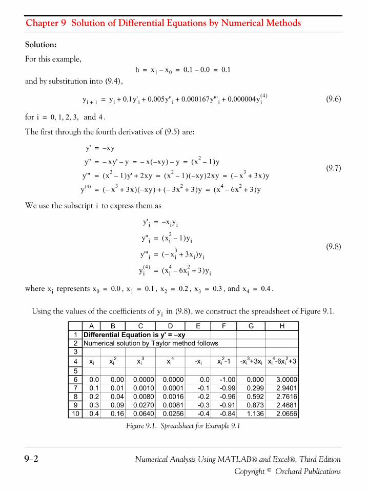
Chapter 9 Solution of Differential Equations by Numerical Methods
9−2 Numerical Analysis Using MATLAB® and Excel®, Third EditionCopyright © Orchard Publications
Solution:
For this example,
and by substitution into (9.4),
(9.6)
for and .
The first through the fourth derivatives of (9.5) are:
(9.7)
We use the subscript to express them as
(9.8)
where represents , , , , and .
Using the values of the coefficients of in (9.8), we construct the spreadsheet of Figure 9.1.
Figure 9.1. Spreadsheet for Example 9.1
h x1 x0– 0.1 0.0– 0.1= = =
yi 1+ yi 0.1y'i 0.005y''i 0.000167y'''i 0.000004yi4( )+ + + +=
i 0 1 2 3 , , , ,= 4
y' xy–=
y'' xy'– y– x xy–( )– y– x2 1–( )y= = =
y''' x2 1–( )y' 2xy+ x2 1–( ) xy–( )2xy x3– 3x+( )y= = =
y 4( ) x3– 3x+( ) xy–( ) 3x2– 3+( )y+ x4 6x2– 3+( )y= =
i
y'i xiyi–=
y''i xi2 1–( )yi=
y'''i xi3– 3xi+( )yi=
yi4( ) xi
4 6xi2– 3+( )yi=
xi x0 0.0= x1 0.1= x2 0.2= x3 0.3= x4 0.4=
yi
123456789
10
A B C D E F G HDifferential Equation is y' = −xy Numerical solution by Taylor method follows
xi xi2 xi
3 xi4 -xi xi
2-1 -xi3+3xi xi
4-6xi2+3
0.0 0.00 0.0000 0.0000 0.0 -1.00 0.000 3.00000.1 0.01 0.0010 0.0001 -0.1 -0.99 0.299 2.94010.2 0.04 0.0080 0.0016 -0.2 -0.96 0.592 2.76160.3 0.09 0.0270 0.0081 -0.3 -0.91 0.873 2.46810.4 0.16 0.0640 0.0256 -0.4 -0.84 1.136 2.0656
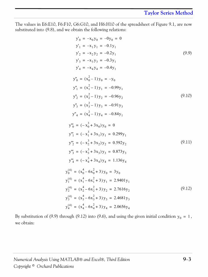
Numerical Analysis Using MATLAB® and Excel®, Third Edition 9−3Copyright © Orchard Publications
Taylor Series Method
The values in E6:E10, F6:F10, G6:G10, and H6:H10 of the spreadsheet of Figure 9.1, are nowsubstituted into (9.8), and we obtain the following relations:
(9.9)
(9.10)
(9.11)
(9.12)
By substitution of (9.9) through (9.12) into (9.6), and using the given initial condition ,we obtain:
y'0 x0 y0– 0y0– 0= = =
y'1 x1 y1– 0.1y1–= =
y'2 x2 y2– 0.2y1–= =
y'3 x3 y3– 0.3y1–= =
y'4 x4 y4– 0.4y1–= =
y''0 x02 1–( ) y0 y0–= =
y''1 x12 1–( ) y1 0.99– y1= =
y''2 x22 1–( ) y2 0.96– y2= =
y''3 x32 1–( ) y3 0.91– y3= =
y''4 x42 1–( ) y4 0.84– y1= =
y'''0 x03– 3x0+( ) y0 0= =
y'''1 x13– 3x1+( ) y1 0.299y1= =
y'''2 x23– 3x2+( ) y2 0.592y2= =
y'''3 x33– 3x3+( ) y3 0.873y3= =
y'''4 x43– 3x4+( ) y4 1.136y4= =
y04( ) x0
4 6x02– 3+( ) y0 3y0= =
y14( ) x1
4 6x12– 3+( ) y1 2.9401y1= =
y24( ) x2
4 6x22– 3+( ) y2 2.7616y2= =
y34( ) x3
4 6x32– 3+( ) y3 2.4681y3= =
y44( ) x4
4 6x42– 3+( ) y4 2.0656y4= =
y0 1=
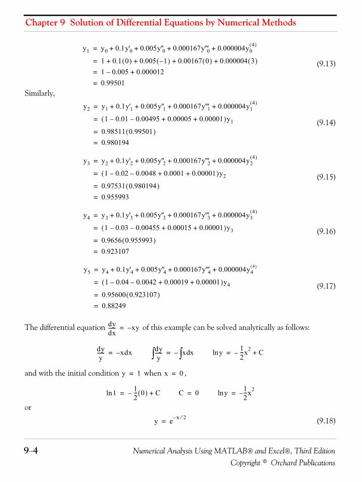
Chapter 9 Solution of Differential Equations by Numerical Methods
9−4 Numerical Analysis Using MATLAB® and Excel®, Third EditionCopyright © Orchard Publications
(9.13)
Similarly,
(9.14)
(9.15)
(9.16)
(9.17)
The differential equation of this example can be solved analytically as follows:
and with the initial condition when ,
or
(9.18)
y1 y0 0.1y'0 0.005y''0 0.000167y'''0 0.000004y04( )+ + + +=
1 0.1 0( ) 0.005 1–( ) 0.00167 0( ) 0.000004 3( )+ + + +=
1 0.005– 0.000012+=
0.99501=
y2 y1 0.1y'1 0.005y''1 0.000167y'''1 0.000004y14( )+ + + +=
1 0.01– 0.00495– 0.00005 0.00001+ +( )y1=
0.98511 0.99501( )=
0.980194=
y3 y2 0.1y'2 0.005y''2 0.000167y'''2 0.000004y24( )+ + + +=
1 0.02– 0.0048– 0.0001 0.00001+ +( )y2=
0.97531 0.980194( )=
0.955993=
y4 y3 0.1y'3 0.005y''3 0.000167y'''3 0.000004y34( )+ + + +=
1 0.03– 0.00455– 0.00015 0.00001+ +( )y3=
0.9656 0.955993( )=
0.923107=
y5 y4 0.1y'4 0.005y''4 0.000167y'''4 0.000004y44( )+ + + +=
1 0.04– 0.0042– 0.00019 0.00001+ +( )y4=
0.95600 0.923107( )=
0.88249=
dydx------ xy–=
dyy
------ xdx–= dyy
------∫ x xd∫–= yln 12---x2– C+=
y 1= x 0=
1ln 12--- 0( )– C+= C 0= yln 1
2---x2–=
y e x 2⁄–=
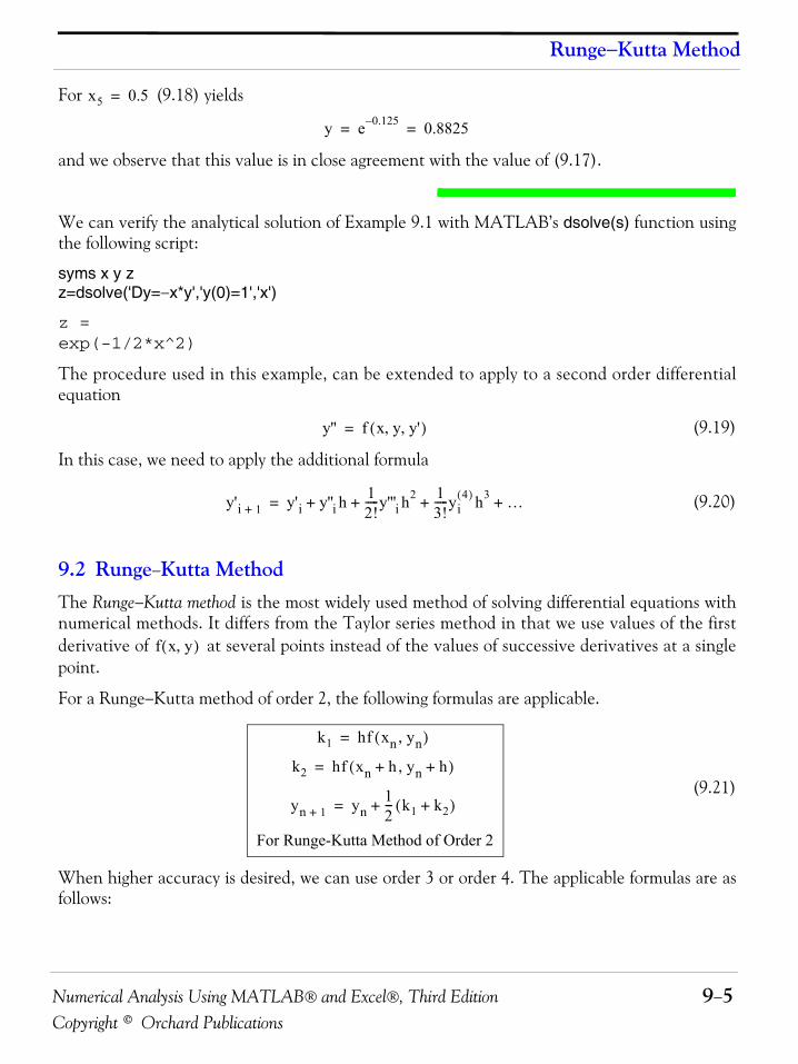
Numerical Analysis Using MATLAB® and Excel®, Third Edition 9−5Copyright © Orchard Publications
Runge−Kutta Method
For (9.18) yields
and we observe that this value is in close agreement with the value of (9.17).
We can verify the analytical solution of Example 9.1 with MATLAB’s dsolve(s) function usingthe following script:
syms x y zz=dsolve('Dy=−x*y','y(0)=1','x')
z =exp(-1/2*x^2)
The procedure used in this example, can be extended to apply to a second order differentialequation
(9.19)
In this case, we need to apply the additional formula
(9.20)
9.2 Runge−Kutta MethodThe Runge−Kutta method is the most widely used method of solving differential equations withnumerical methods. It differs from the Taylor series method in that we use values of the firstderivative of at several points instead of the values of successive derivatives at a singlepoint.
For a Runge−Kutta method of order 2, the following formulas are applicable.
(9.21)
When higher accuracy is desired, we can use order 3 or order 4. The applicable formulas are asfollows:
x5 0.5=
y e 0.125– 0.8825= =
y'' f x y y', ,( )=
y'i 1+ y'i y''i h 12!-----y'''i h2 1
3!-----yi
4( ) h3 …+ + + +=
f x y,( )
k1 hf xn yn,( )=
k2 hf xn h+ yn h+,( )=
yn 1+ yn12--- k1 k2+( )+=
For Runge-Kutta Method of Order 2
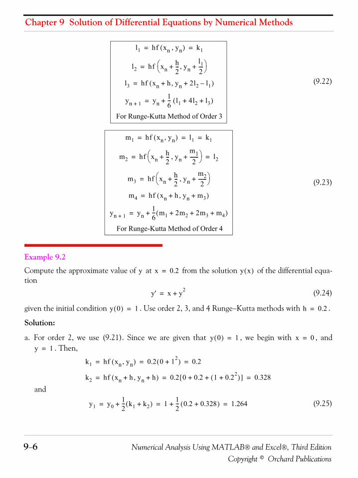
Chapter 9 Solution of Differential Equations by Numerical Methods
9−6 Numerical Analysis Using MATLAB® and Excel®, Third EditionCopyright © Orchard Publications
(9.22)
(9.23)
Example 9.2
Compute the approximate value of at from the solution of the differential equa-tion
(9.24)
given the initial condition . Use order 2, 3, and 4 Runge−Kutta methods with .
Solution:
a. For order 2, we use (9.21). Since we are given that , we begin with , and. Then,
and
(9.25)
l1 hf xn yn,( ) k1= =
l2 hf xnh2---+ yn
l12----+,⎝ ⎠
⎛ ⎞=
l3 hf xn h+ yn 2l2 l1–+,( )=
yn 1+ yn16--- l1 4l2 l3+ +( )+=
For Runge-Kutta Method of Order 3
m1 hf xn yn,( ) l1 k1= = =
m2 hf xnh2---+ yn
m12
-------+,⎝ ⎠⎛ ⎞ l2= =
m3 hf xnh2---+ yn
m22
-------+,⎝ ⎠⎛ ⎞=
m4 hf xn h+ yn m3+,( )=
yn 1+ yn16--- m1 2m2 2m3 m4+ + +( )+=
For Runge-Kutta Method of Order 4
y x 0.2= y x( )
y' x y2+=
y 0( ) 1= h 0.2=
y 0( ) 1= x 0=
y 1=
k1 hf xn yn,( ) 0.2 0 12+( ) 0.2= = =
k2 hf xn h+ yn h+,( ) 0.2 0 0.2 1 0.22+( )+ +[ ] 0.328= = =
y1 y012--- k1 k2+( )+ 1 1
2--- 0.2 0.328+( )+ 1.264= = =
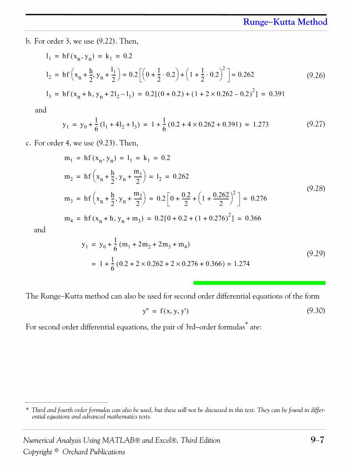
Numerical Analysis Using MATLAB® and Excel®, Third Edition 9−7Copyright © Orchard Publications
Runge−Kutta Method
b. For order 3, we use (9.22). Then,
(9.26)
and
(9.27)
c. For order 4, we use (9.23). Then,
(9.28)
and
(9.29)
The Runge−Kutta method can also be used for second order differential equations of the form
(9.30)
For second order differential equations, the pair of 3rd−order formulas* are:
* Third and fourth order formulas can also be used, but these will not be discussed in this text. They can be found in differ-ential equations and advanced mathematics texts.
l1 hf xn yn,( ) k1 0.2= = =
l2 hf xnh2---+ yn
l12----+,⎝ ⎠
⎛ ⎞ 0.2 0 12--- 0.2⋅+⎝ ⎠
⎛ ⎞ 1 12--- 0.2⋅+⎝ ⎠
⎛ ⎞ 2+ 0.262= ==
l3 hf xn h+ yn 2l2 l1–+,( ) 0.2 0 0.2+( ) 1 2 0.262 0.2–×+( )2+[ ] 0.391= = =
y1 y016--- l1 4l2 l3+ +( )+ 1 1
6--- 0.2 4 0.262 0.391+×+( )+ 1.273= = =
m1 hf xn yn,( ) l1 k1 0.2= = = =
m2 hf xnh2---+ yn
m12
-------+,⎝ ⎠⎛ ⎞ l2 0.262= = =
m3 hf xnh2---+ yn
m22
-------+,⎝ ⎠⎛ ⎞ 0.2 0 0.2
2------- 1 0.262
2-------------+⎝ ⎠
⎛ ⎞ 2+ + 0.276= = =
m4 hf xn h+ yn m3+,( ) 0.2 0 0.2 1 0.276+( )2+ +[ ] 0.366= = =
y1 y016--- m1 2m2 2m3 m4+ + +( )+=
1 16--- 0.2 2 0.262 2 0.276 0.366+×+×+( )+ 1.274==
y'' f x y y', ,( )=
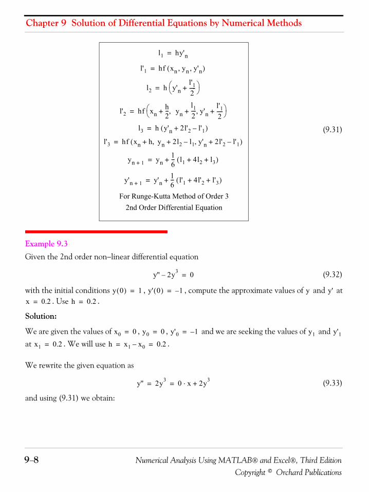
Chapter 9 Solution of Differential Equations by Numerical Methods
9−8 Numerical Analysis Using MATLAB® and Excel®, Third EditionCopyright © Orchard Publications
(9.31)
Example 9.3 Given the 2nd order non−linear differential equation
(9.32)
with the initial conditions , , compute the approximate values of and at. Use .
Solution:
We are given the values of , , and we are seeking the values of and at . We will use .
We rewrite the given equation as
(9.33)
and using (9.31) we obtain:
l1 hy'n=
l'1 hf xn yn y'n, ,( ) =
l2 h y'nl'12-----+⎝ ⎠
⎛ ⎞=
l'2 hf xnh2--- yn
l12---- y'n,+,
l'12-----+ +⎝ ⎠
⎛ ⎞=
l3 h y'n 2l'2 l'1–+( )=
l'3 hf xn h yn 2l2 l1– y'n,+, 2l'2 l'1–+ +( )=
yn 1+ yn16--- l1 4l2 l3+ +( )+=
y'n 1+ y'n16--- l'1 4l'2 l'3+ +( )+=
For Runge-Kutta Method of Order 3 2nd Order Differential Equation
y'' 2y3– 0=
y 0( ) 1= y' 0( ) 1–= y y'x 0.2= h 0.2=
x0 0= y0 0= y'0 1–= y1 y'1x1 0.2= h x1 x0– 0.2= =
y'' 2y3 0 x⋅ 2y3+= =
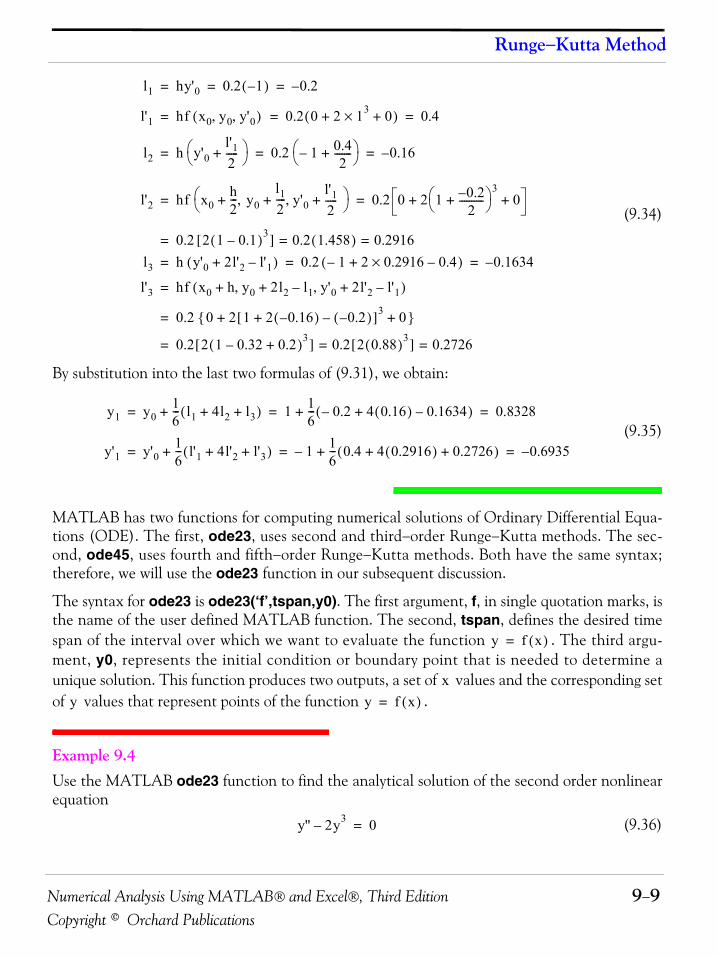
Numerical Analysis Using MATLAB® and Excel®, Third Edition 9−9Copyright © Orchard Publications
Runge−Kutta Method
(9.34)
By substitution into the last two formulas of (9.31), we obtain:
(9.35)
MATLAB has two functions for computing numerical solutions of Ordinary Differential Equa-tions (ODE). The first, ode23, uses second and third−order Runge−Kutta methods. The sec-ond, ode45, uses fourth and fifth−order Runge−Kutta methods. Both have the same syntax;therefore, we will use the ode23 function in our subsequent discussion.
The syntax for ode23 is ode23(‘f’,tspan,y0). The first argument, f, in single quotation marks, isthe name of the user defined MATLAB function. The second, tspan, defines the desired timespan of the interval over which we want to evaluate the function . The third argu-ment, y0, represents the initial condition or boundary point that is needed to determine aunique solution. This function produces two outputs, a set of values and the corresponding setof values that represent points of the function .
Example 9.4 Use the MATLAB ode23 function to find the analytical solution of the second order nonlinearequation
(9.36)
l1 hy'0 0.2 1–( ) 0.2–= = =
l'1 hf x0 y0 y'0, ,( ) 0.2 0 2 13× 0+ +( ) 0.4= = =
l2 h y'0l'12-----+⎝ ⎠
⎛ ⎞ 0.2 1– 0.42
-------+⎝ ⎠⎛ ⎞ 0.16–= = =
l'2 hf x0h2--- y0
l12---- y'0,+,
l'12-----+ +⎝ ⎠
⎛ ⎞ 0.2 0 2 1 0.2–2
----------+⎝ ⎠⎛ ⎞ 3
0+ += =
0.2 2 1 0.1–( )3[ ] 0.2 1.458( )= 0.2916==
l3 h y'0 2l'2 l'1–+( ) 0.2 1– 2 0.2916 0.4–×+( ) 0.1634–= = =
l'3 hf x0 h y0 2l2 l1– y'0,+, 2l'2 l'1–+ +( )=
0.2 0 2 1 2 0.16–( ) 0.2–( )–+[ ]3 0+ +{ }=
0.2 2 1 0.32– 0.2+( )3[ ] 0.2 2 0.88( )3[ ] 0.2726= ==
y1 y016--- l1 4l2 l3+ +( )+ 1 1
6--- 0.2– 4 0.16( ) 0.1634–+( )+ 0.8328= = =
y'1 y'016--- l'1 4l'2 l'3+ +( )+ 1–
16--- 0.4 4 0.2916( ) 0.2726+ +( )+ 0.6935–= = =
y f x( )=
xy y f x( )=
y'' 2y3– 0=
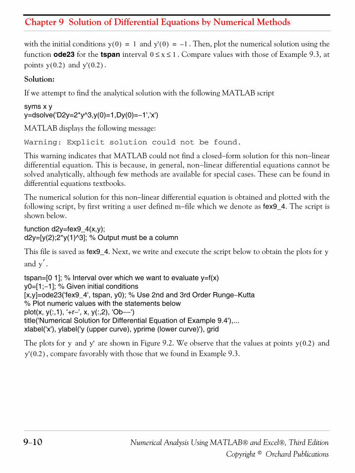
Chapter 9 Solution of Differential Equations by Numerical Methods
9−10 Numerical Analysis Using MATLAB® and Excel®, Third EditionCopyright © Orchard Publications
with the initial conditions and . Then, plot the numerical solution using thefunction ode23 for the tspan interval . Compare values with those of Example 9.3, atpoints and .
Solution:
If we attempt to find the analytical solution with the following MATLAB script
syms x yy=dsolve('D2y=2*y^3,y(0)=1,Dy(0)=−1','x')
MATLAB displays the following message:
Warning: Explicit solution could not be found.
This warning indicates that MATLAB could not find a closed−form solution for this non−lineardifferential equation. This is because, in general, non−linear differential equations cannot besolved analytically, although few methods are available for special cases. These can be found indifferential equations textbooks.
The numerical solution for this non−linear differential equation is obtained and plotted with thefollowing script, by first writing a user defined m−file which we denote as fex9_4. The script isshown below.
function d2y=fex9_4(x,y);d2y=[y(2);2*y(1)^3]; % Output must be a column
This file is saved as fex9_4. Next, we write and execute the script below to obtain the plots for
and .
tspan=[0 1]; % Interval over which we want to evaluate y=f(x)y0=[1;−1]; % Given initial conditions[x,y]=ode23('fex9_4', tspan, y0); % Use 2nd and 3rd Order Runge−Kutta% Plot numeric values with the statements belowplot(x, y(:,1), '+r−', x, y(:,2), 'Ob−−')title('Numerical Solution for Differential Equation of Example 9.4'),...xlabel('x'), ylabel('y (upper curve), yprime (lower curve)'), grid
The plots for and are shown in Figure 9.2. We observe that the values at points and, compare favorably with those that we found in Example 9.3.
y 0( ) 1= y' 0( ) 1–=
0 x 1≤ ≤y 0.2( ) y' 0.2( )
y
y ′
y y' y 0.2( )y' 0.2( )
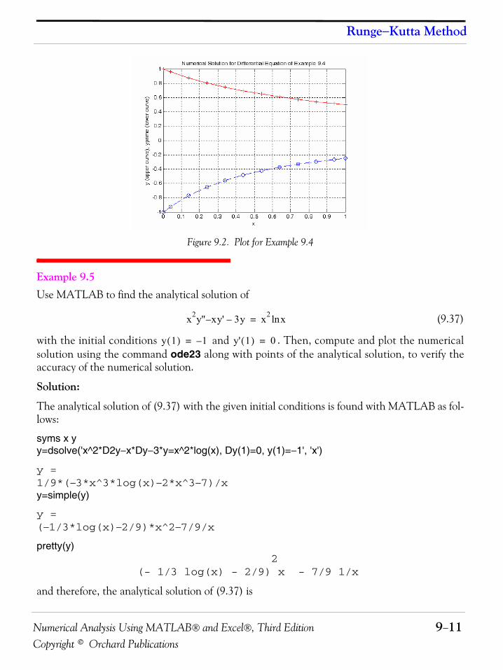
Numerical Analysis Using MATLAB® and Excel®, Third Edition 9−11Copyright © Orchard Publications
Runge−Kutta Method
Figure 9.2. Plot for Example 9.4
Example 9.5 Use MATLAB to find the analytical solution of
(9.37)
with the initial conditions and . Then, compute and plot the numericalsolution using the command ode23 along with points of the analytical solution, to verify theaccuracy of the numerical solution.
Solution:
The analytical solution of (9.37) with the given initial conditions is found with MATLAB as fol-lows:
syms x y y=dsolve('x^2*D2y−x*Dy−3*y=x^2*log(x), Dy(1)=0, y(1)=−1', 'x')
y =1/9*(−3*x^3*log(x)−2*x^3−7)/xy=simple(y)
y =(−1/3*log(x)−2/9)*x^2−7/9/x
pretty(y) 2 (- 1/3 log(x) - 2/9) x - 7/9 1/x
and therefore, the analytical solution of (9.37) is
x2y'' x– y' 3y– x2 xln=
y 1( ) 1–= y' 1( ) 0=
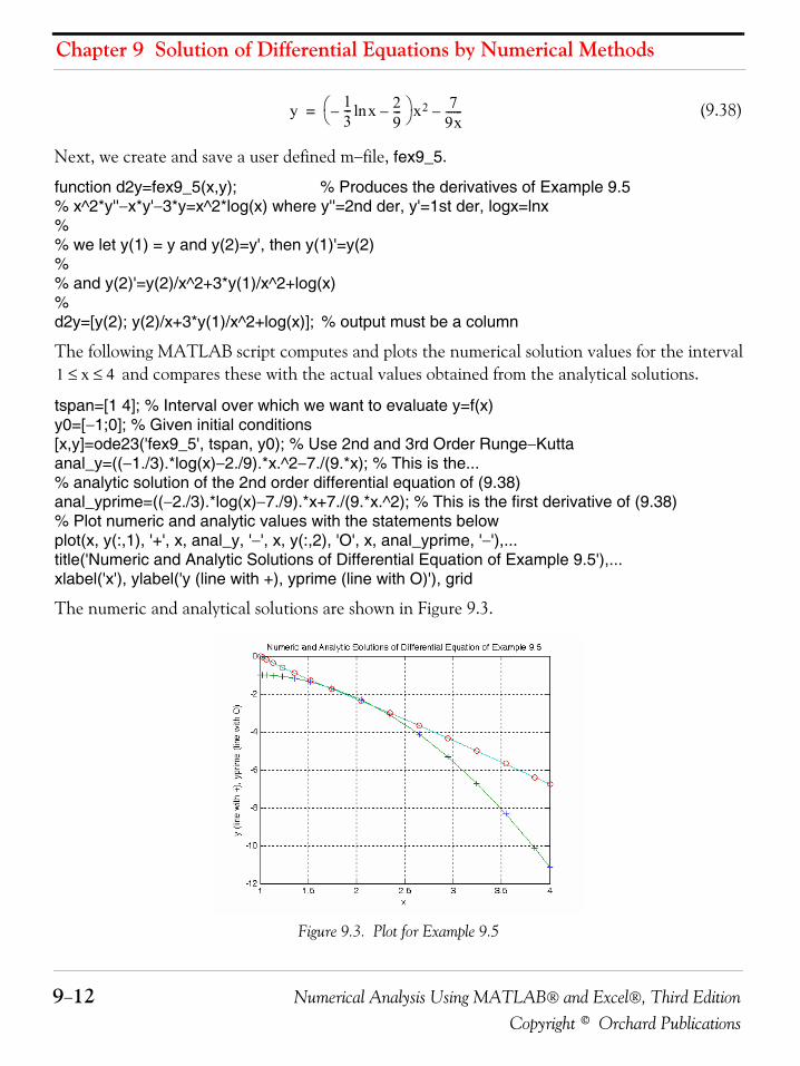
Chapter 9 Solution of Differential Equations by Numerical Methods
9−12 Numerical Analysis Using MATLAB® and Excel®, Third EditionCopyright © Orchard Publications
(9.38)
Next, we create and save a user defined m−file, fex9_5.
function d2y=fex9_5(x,y); % Produces the derivatives of Example 9.5% x^2*y''−x*y'−3*y=x^2*log(x) where y''=2nd der, y'=1st der, logx=lnx%% we let y(1) = y and y(2)=y', then y(1)'=y(2)%% and y(2)'=y(2)/x^2+3*y(1)/x^2+log(x)%d2y=[y(2); y(2)/x+3*y(1)/x^2+log(x)]; % output must be a column
The following MATLAB script computes and plots the numerical solution values for the interval and compares these with the actual values obtained from the analytical solutions.
tspan=[1 4]; % Interval over which we want to evaluate y=f(x)y0=[−1;0]; % Given initial conditions[x,y]=ode23('fex9_5', tspan, y0); % Use 2nd and 3rd Order Runge−Kuttaanal_y=((−1./3).*log(x)−2./9).*x.^2−7./(9.*x); % This is the...% analytic solution of the 2nd order differential equation of (9.38)anal_yprime=((−2./3).*log(x)−7./9).*x+7./(9.*x.^2); % This is the first derivative of (9.38)% Plot numeric and analytic values with the statements belowplot(x, y(:,1), '+', x, anal_y, '−', x, y(:,2), 'O', x, anal_yprime, '−'),...title('Numeric and Analytic Solutions of Differential Equation of Example 9.5'),...xlabel('x'), ylabel('y (line with +), yprime (line with O)'), grid
The numeric and analytical solutions are shown in Figure 9.3.
Figure 9.3. Plot for Example 9.5
y 13--- xln– 2
9---–⎝ ⎠
⎛ ⎞ x2 79x------–=
1 x 4≤ ≤
Numerical Analysis Using MATLAB® and Excel®, Third Edition 9−13Copyright © Orchard Publications
Adams’ Method
9.3 Adams’ Method
In this method, the step from to is performed by a formula expressed in terms of differ-
ences of .
Adams’ method uses the formula
(9.39)
where
and so on.
Obviously, to form a table of differences, it is necessary to have several (4 or more) approximatevalues of in addition to the given initial condition . These values can be found byother methods such as the Taylor series or Runge−Kutta methods.
Example 9.6 Given the differential equation
(9.40)with the initial condition ,
compute the approximate values of y for by the third−orderRunge−Kutta method. Then, find the value of corresponding to correct to three dec-imal places using Adams’ method.
Solution:
The spreadsheet of Figure 9.4 shows the results of the computations of using the third−order Runge−Kutta method as in Example 9.2.
yn yn 1+
f x y,( )
yn 1+ yn h fn12---Δfn
512------Δ2fn
38---Δ3fn …+ + + ++=
h xn 1+ xn–=
fn xn yn,( )=
Δfn fn fn 1––=
Δ2fn Δfn Δfn 1––=
y x( ) y 0( )
y' 2y x+=
y 0( ) 1=
x 0.1 0.2 0.3 0.4 and 0.5 , , ,=
y x 0.6=
y1 y2 y3 y4,, , , and y5
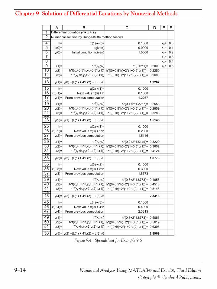
Chapter 9 Solution of Differential Equations by Numerical Methods
9−14 Numerical Analysis Using MATLAB® and Excel®, Third EditionCopyright © Orchard Publications
Figure 9.4. Spreadsheet for Example 9.6
123456789
1011121314151617181920212223242526272829303132333435363738394041424344454647484950515253
A B C D E FDifferential Equation y' = x + 2yNumerical solution by Runga-Kutte method follows
h= x(1)-x(0)= 0.1000 x0= 0.0x(0)= (given) 0.0000 x1= 0.1y(0)= Initial condition (given) 1.0000 x2= 0.2
x3= 0.3x4= 0.4
L(1)= h*f(xn,yn) h*(0+2*1)= 0.2000 x5= 0.5L(2)= h*f(xn+0.5*h,yn+0.5*L(1)) h*[(0+0.5*h)+2*(1+0.5*L(1))]= 0.2250L(3)= h*f(xn+h,yn+2*L(2)-L(1)) h*[(0+h)+2*(1+2*L(2)-L(1))]= 0.2600
y(1)= y(0) +(L(1) + 4*L(2) + L(3))/6 1.2267
h= x(2)-x(1)= 0.1000x(0.1)= Next value x(0) + h 0.1000
y(1)= From previous computation 1.2267
L(1)= h*f(xn,yn) h*(0.1+2*1.2267)= 0.2553L(2)= h*f(xn+0.5*h,yn+0.5*L(1)) h*[(0+0.5*h)+2*(1+0.5*L(1))]= 0.2859L(3)= h*f(xn+h,yn+2*L(2)-L(1)) h*[(0+h)+2*(1+2*L(2)-L(1))]= 0.3286
y(2)= y(1) +(L(1) + 4*L(2) + L(3))/6 1.5146
h= x(2)-x(1)= 0.1000x(0.2)= Next value x(0) + 2*h 0.2000
y(2)= From previous computation 1.5146
L(1)= h*f(xn,yn) h*(0.2+2*1.5146)= 0.3229L(2)= h*f(xn+0.5*h,yn+0.5*L(1)) h*[(0+0.5*h)+2*(1+0.5*L(1))]= 0.3602L(3)= h*f(xn+h,yn+2*L(2)-L(1)) h*[(0+h)+2*(1+2*L(2)-L(1))]= 0.4124
y(3)= y(2) +(L(1) + 4*L(2) + L(3))/6 1.8773
h= x(3)-x(2)= 0.1000x(0.3)= Next value x(0) + 3*h 0.3000
y(3)= From previous computation 1.8773
L(1)= h*f(xn,yn) h*(0.3+2*1.8773)= 0.4055L(2)= h*f(xn+0.5*h,yn+0.5*L(1)) h*[(0+0.5*h)+2*(1+0.5*L(1))]= 0.4510L(3)= h*f(xn+h,yn+2*L(2)-L(1)) h*[(0+h)+2*(1+2*L(2)-L(1))]= 0.5148
y(4)= y(2) +(L(1) + 4*L(2) + L(3))/6 2.3313
h= x(4)-x(3)= 0.1000x(0.4)= Next value x(0) + 4*h 0.4000
y(4)= From previous computation 2.3313
L(1)= h*f(xn,yn) h*(0.3+2*1.8773)= 0.5063L(2)= h*f(xn+0.5*h,yn+0.5*L(1)) h*[(0+0.5*h)+2*(1+0.5*L(1))]= 0.5619L(3)= h*f(xn+h,yn+2*L(2)-L(1)) h*[(0+h)+2*(1+2*L(2)-L(1))]= 0.6398
y(5)= y(2) +(L(1) + 4*L(2) + L(3))/6 2.8969
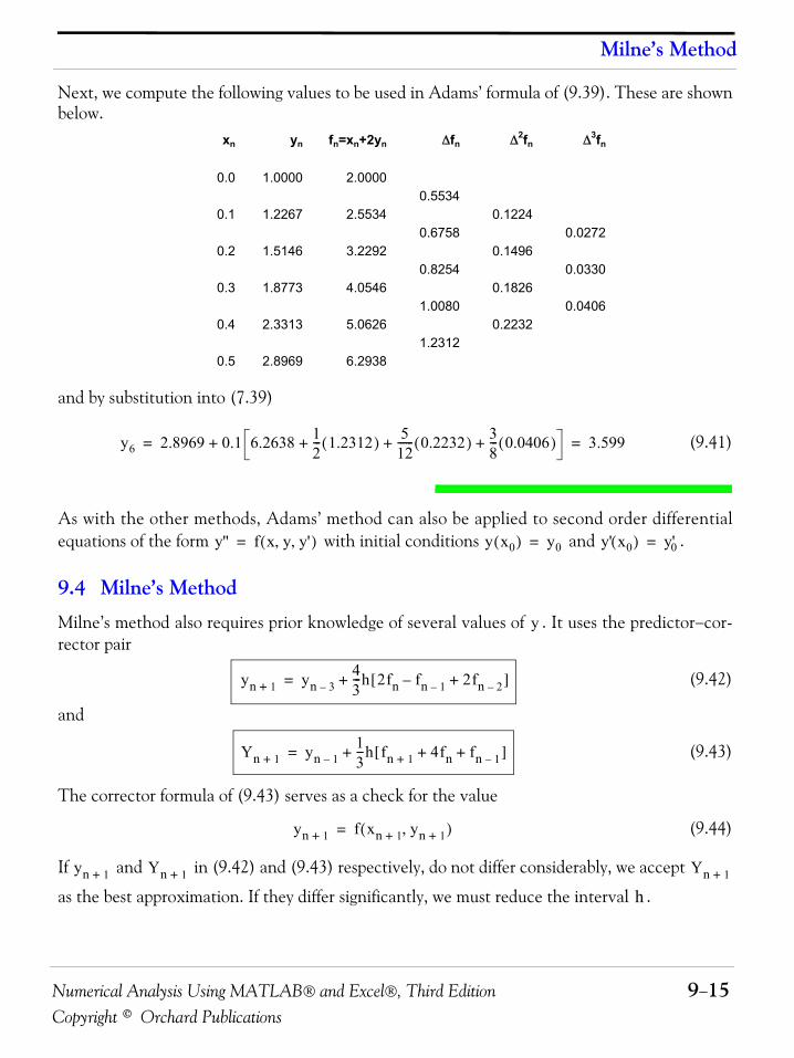
Numerical Analysis Using MATLAB® and Excel®, Third Edition 9−15Copyright © Orchard Publications
Milne’s Method
Next, we compute the following values to be used in Adams’ formula of (9.39). These are shownbelow.
and by substitution into (7.39)
(9.41)
As with the other methods, Adams’ method can also be applied to second order differentialequations of the form with initial conditions and .
9.4 Milne’s Method
Milne’s method also requires prior knowledge of several values of . It uses the predictor−cor-rector pair
(9.42)
and
(9.43)
The corrector formula of (9.43) serves as a check for the value
(9.44)
If and in (9.42) and (9.43) respectively, do not differ considerably, we accept
as the best approximation. If they differ significantly, we must reduce the interval .
xn yn fn=xn+2yn Δfn Δ2fn Δ3fn
0.0 1.0000 2.00000.5534
0.1 1.2267 2.5534 0.12240.6758 0.0272
0.2 1.5146 3.2292 0.14960.8254 0.0330
0.3 1.8773 4.0546 0.18261.0080 0.0406
0.4 2.3313 5.0626 0.22321.2312
0.5 2.8969 6.2938
y6 2.8969 0.1 6.2638 12--- 1.2312( ) 5
12------ 0.2232( ) 3
8--- 0.0406( )+ + ++ 3.599= =
y'' f x y y', ,( )= y x0( ) y0= y' x0( ) y'0=
y
yn 1+ yn 3–43---h 2fn fn 1–– 2fn 2–+[ ]+=
Yn 1+ yn 1–13---h fn 1+ 4fn fn 1–+ +[ ]+=
yn 1+ f xn 1+ yn 1+,( )=
yn 1+ Yn 1+ Yn 1+
h
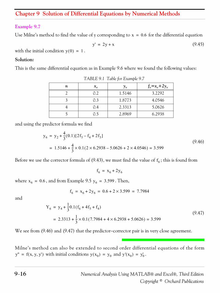
Chapter 9 Solution of Differential Equations by Numerical Methods
9−16 Numerical Analysis Using MATLAB® and Excel®, Third EditionCopyright © Orchard Publications
Example 9.7
Use Milne’s method to find the value of y corresponding to for the differential equation
(9.45)with the initial condition .
Solution:
This is the same differential equation as in Example 9.6 where we found the following values:
and using the predictor formula we find
(9.46)
Before we use the corrector formula of (9.43), we must find the value of ; this is found from
where , and from Example 9.5 . Then,
and
(9.47)
We see from (9.46) and (9.47) that the predictor−corrector pair is in very close agreement.
Milne’s method can also be extended to second order differential equations of the form with initial conditions and .
TABLE 9.1 Table for Example 9.7
n xn yn fn=xn+2yn
2 0.2 1.5146 3.2292
3 0.3 1.8773 4.0546
4 0.4 2.3313 5.0626
5 0.5 2.8969 6.2938
x 0.6=
y' 2y x+=
y 0( ) 1=
y6 y243--- 0.1( ) 2f5 f4– 2f3+[ ]+=
1.5146 43--- 0.1 2 6.2938 5.0626– 2 4.0546×+×( )×+ 3.599==
f6
f6 x6 2y6+=
x6 0.6= y6 3.599=
f6 x6 2y6+ 0.6 2 3.599×+ 7.7984= = =
Y6 y413---0.1 f6 4f5 f4+ +( )+=
2.3313 13--- 0.1 7.7984 4 6.2938 5.0626+×+( )×+ 3.599==
y'' f x y y', ,( )= y x0( ) y0= y' x0( ) y'0=
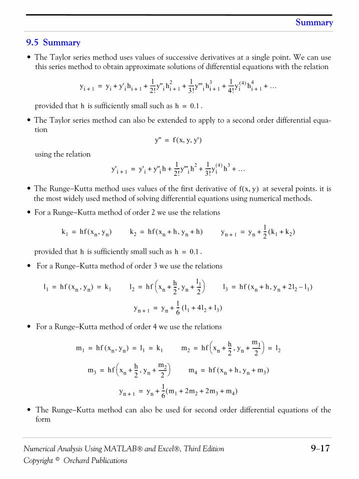
Numerical Analysis Using MATLAB® and Excel®, Third Edition 9−17Copyright © Orchard Publications
Summary
9.5 Summary• The Taylor series method uses values of successive derivatives at a single point. We can use
this series method to obtain approximate solutions of differential equations with the relation
provided that is sufficiently small such as .
• The Taylor series method can also be extended to apply to a second order differential equa-tion
using the relation
• The Runge−Kutta method uses values of the first derivative of at several points. it isthe most widely used method of solving differential equations using numerical methods.
• For a Runge−Kutta method of order 2 we use the relations
provided that is sufficiently small such as .
• For a Runge−Kutta method of order 3 we use the relations
• For a Runge−Kutta method of order 4 we use the relations
• The Runge−Kutta method can also be used for second order differential equations of theform
yi 1+ yi y'i hi 1+12!-----y''i hi 1+
2 13!-----y'''i hi 1+
3 14!-----yi
4( ) hi 1+4 …+ + + + +=
h h 0.1=
y'' f x y y', ,( )=
y'i 1+ y'i y''i h 12!-----y'''i h2 1
3!-----yi
4( ) h3 …+ + + +=
f x y,( )
k1 hf xn yn,( )= k2 hf xn h+ yn h+,( )= yn 1+ yn12--- k1 k2+( )+=
h h 0.1=
l1 hf xn yn,( ) k1= = l2 hf xnh2---+ yn
l12----+,⎝ ⎠
⎛ ⎞= l3 hf xn h+ yn 2l2 l1–+,( )=
yn 1+ yn16--- l1 4l2 l3+ +( )+=
m1 hf xn yn,( ) l1 k1= = = m2 hf xnh2---+ yn
m12
-------+,⎝ ⎠⎛ ⎞ l2= =
m3 hf xnh2---+ yn
m22
-------+,⎝ ⎠⎛ ⎞= m4 hf xn h+ yn m3+,( )=
yn 1+ yn16--- m1 2m2 2m3 m4+ + +( )+=
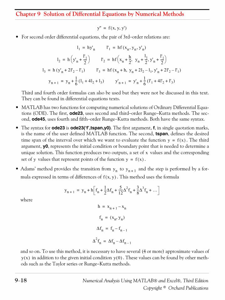
Chapter 9 Solution of Differential Equations by Numerical Methods
9−18 Numerical Analysis Using MATLAB® and Excel®, Third EditionCopyright © Orchard Publications
• For second order differential equations, the pair of 3rd−order relations are:
Third and fourth order formulas can also be used but they were not be discussed in this text.They can be found in differential equations texts.
• MATLAB has two functions for computing numerical solutions of Ordinary Differential Equa-tions (ODE). The first, ode23, uses second and third−order Runge−Kutta methods. The sec-ond, ode45, uses fourth and fifth−order Runge−Kutta methods. Both have the same syntax.
• The syntax for ode23 is ode23(‘f’,tspan,y0). The first argument, f, in single quotation marks,is the name of the user defined MATLAB function. The second, tspan, defines the desiredtime span of the interval over which we want to evaluate the function . The thirdargument, y0, represents the initial condition or boundary point that is needed to determine aunique solution. This function produces two outputs, a set of values and the correspondingset of values that represent points of the function .
• Adams’ method provides the transition from to and the step is performed by a for-
mula expressed in terms of differences of . This method uses the formula
where
and so on. To use this method, it is necessary to have several (4 or more) approximate values of in addition to the given initial condition . These values can be found by other meth-
ods such as the Taylor series or Runge−Kutta methods.
y'' f x y y', ,( )=
l1 hy'n= l'1 hf xn yn y'n, ,( ) =
l2 h y'nl'12-----+⎝ ⎠
⎛ ⎞= l'2 hf xnh2--- yn
l12---- y'n,+,
l'12-----+ +⎝ ⎠
⎛ ⎞=
l3 h y'n 2l'2 l'1–+( )= l'3 hf xn h yn 2l2 l1– y'n,+, 2l'2 l'1–+ +( )=
yn 1+ yn16--- l1 4l2 l3+ +( )+= y'n 1+ y'n
16--- l'1 4l'2 l'3+ +( )+=
y f x( )=
xy y f x( )=
yn yn 1+
f x y,( )
yn 1+ yn h fn12---Δfn
512------Δ2fn
38---Δ3fn …+ + + ++=
h xn 1+ xn–=
fn xn yn,( )=
Δfn fn fn 1––=
Δ2fn Δfn Δfn 1––=
y x( ) y 0( )
Numerical Analysis Using MATLAB® and Excel®, Third Edition 9−19Copyright © Orchard Publications
Summary
• Milne’s method also requires prior knowledge of several values of . It uses the predictor−cor-rector pair
and
where is the predictor formula and is the corrector formula. The corrector for-mula serves as a check for the value
If and do not differ considerably, we accept as the best approximation. If
they differ significantly, we must reduce the interval .
Milne’s method can also be extended to second order differential equations of the form with initial conditions and . The procedure for this
method was not discussed. It can be found in differential equations texts.
y
yn 1+ yn 3–43---h 2fn fn 1–– 2fn 2–+[ ]+=
Yn 1+ yn 1–13---h fn 1+ 4fn fn 1–+ +[ ]+=
yn 1+ Yn 1+
yn 1+ f xn 1+ yn 1+,( )=
yn 1+ Yn 1+ Yn 1+
h
y'' f x y y', ,( )= y x0( ) y0= y' x0( ) y'0=
Chapter 9 Solution of Differential Equations by Numerical Methods
9−20 Numerical Analysis Using MATLAB® and Excel®, Third EditionCopyright © Orchard Publications
9.6 Exercises1. Use the MATLAB ode23 function to verify the analytical solution of Example 9.1.
2. Construct a spreadsheet for the numerical solutions of Example 9.2.
3. Use MATLAB to find the analytical solution of
with the initial condition . Then, compute and plot the numerical solution usingthe MATLAB function ode23 along with points of the analytical solution to verify the accu-racy of the numerical solution for the interval .
4. Use MATLAB to plot the numerical solution of the non−linear differential equation
with the initial condition using the command ode23 for the interval .
5. Given the differential equation
with the initial condition and find the values of corresponding to thevalues of and correct to four decimal places using the third−order Runge−Kutta method. It is suggested that a spreadsheet is used to do all computations.
6. Given the differential equation
compute the approximate values of and at and given that ,, and correct to four decimal places, using the third−order Runge−Kutta
method. It is suggested that a spreadsheet is used to do all computations.
y' f x( ) 3x2= =
y 2( ) 0.5=
2 x 4≤ ≤
y' y3– 0.2 xsin+=
y 0( ) 0.707= 0 x 10≤ ≤
y' x2 y–=
y 0( ) 1= x0 0.0= y
x0 0.1+ x0 0.2+
y'' y'+ xy=
y y' x0 0.1+ x0 0.2+ y 0( ) 1=
y' 0( ) 1–= x0 0.0=
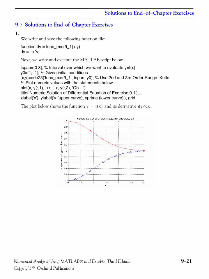
Numerical Analysis Using MATLAB® and Excel®, Third Edition 9−21Copyright © Orchard Publications
Solutions to End−of−Chapter Exercises
9.7 Solutions to End−of−Chapter Exercises1.
We write and save the following function file:
function dy = func_exer9_1(x,y)dy = −x*y;
Next, we write and execute the MATLAB script below.
tspan=[0 3]; % Interval over which we want to evaluate y=f(x)y0=[1;−1]; % Given initial conditions[x,y]=ode23('func_exer9_1', tspan, y0); % Use 2nd and 3rd Order Runge−Kutta% Plot numeric values with the statements belowplot(x, y(:,1), '+r−', x, y(:,2), 'Ob−−')title('Numeric Solution of Differential Equation of Exercise 9.1'),...xlabel('x'), ylabel('y (upper curve), yprime (lower curve)'), grid
The plot below shows the function and its derivative .y f x( )= dy dx⁄
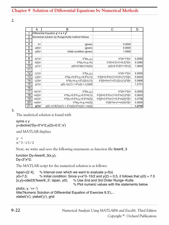
Chapter 9 Solution of Differential Equations by Numerical Methods
9−22 Numerical Analysis Using MATLAB® and Excel®, Third EditionCopyright © Orchard Publications
2.
3.The analytical solution is found with
syms x yy=dsolve('Dy=3*x^2,y(2)=0.5','x')
and MATLAB displays
y =x^3-15/2
Next, we write and save the following statements as function file fexer9_3
function Dy=fexer9_3(x,y);Dy=3*x^2;
The MATLAB script for the numerical solution is as follows:
tspan=[2 4]; % Interval over which we want to evaluate y=f(x)y0=7.5; % Initial condition: Since y=x^3−15/2 and y(2) = 0.5, it follows that y(0) = 7.5[x,y]=ode23('fexer9_3', tspan, y0); % Use 2nd and 3rd Order Runge−Kutta
% Plot numeric values with the statements belowplot(x, y, '+r−')title('Numeric Solution of Differential Equation of Exercise 9.3'),...xlabel('x'), ylabel('y'), grid
123456789101112131415161718192021
A B C DDifferential Equation y' = x + y2
Numerical solution by Runga-Kutte method follows
h= (given) 0.2000x(0)= (given) 0.0000y(0)= Initial condition (given) 1.0000
k(1)= h*f(xn,yn) h*(0+1^2)= 0.2000k(2)= h*f(xn+h,yn+h) h*(0+0.2+(1+0.2)^2)= 0.3280y(1)= y(0)+0.5(k(1)+k(2)) y(0)+0.5*(D11+D12) 1.2640
L(1)= h*f(xn,yn) h*(0+1^2)= 0.2000L(2)= h*f(xn+0.5*h,yn+0.5*L(1)) h*[(0+0.5*h)+(1+0.5*L(1)^2)]= 0.2620L(3)= h*f(xn+h,yn+2*L(2)-L(1)) h*[(0+h)+(1+2*L(2)-L(1))^2]= 0.3906y(1)= y(0) +(L(1) + 4*L(2) + L(3))/6 1.2731
m(1)= h*f(xn,yn) h*(0+1^2)= 0.2000m(2)= h*f(xn+0.5*h,yn+0.5*m(1)) h*[(0+0.5*h)+(1+0.5*m(1))^2]= 0.2620m(3)= h*f(xn+0.5*h,yn+0.5*m(2)) h*[(0+0.5*h)+(1+0.5*m(2))^2]= 0.2758m(4)= h*f(xn+h,yn+m(3)) h*[(0+h)+(1+m(3))^2]= 0.3655y(1)= y(0) +(1/6)*(m(1) + 2*m(2)+2*m(3) + m(4)) 1.2735
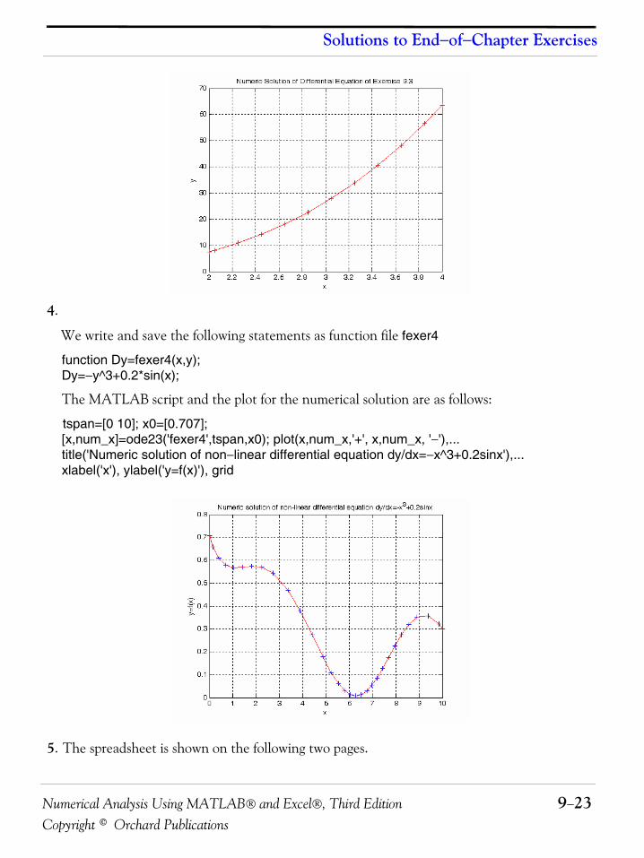
Numerical Analysis Using MATLAB® and Excel®, Third Edition 9−23Copyright © Orchard Publications
Solutions to End−of−Chapter Exercises
4.
We write and save the following statements as function file fexer4
function Dy=fexer4(x,y);Dy=−y^3+0.2*sin(x);
The MATLAB script and the plot for the numerical solution are as follows:
tspan=[0 10]; x0=[0.707];[x,num_x]=ode23('fexer4',tspan,x0); plot(x,num_x,'+', x,num_x, '−'),...title('Numeric solution of non−linear differential equation dy/dx=−x^3+0.2sinx'),...xlabel('x'), ylabel('y=f(x)'), grid
5. The spreadsheet is shown on the following two pages.
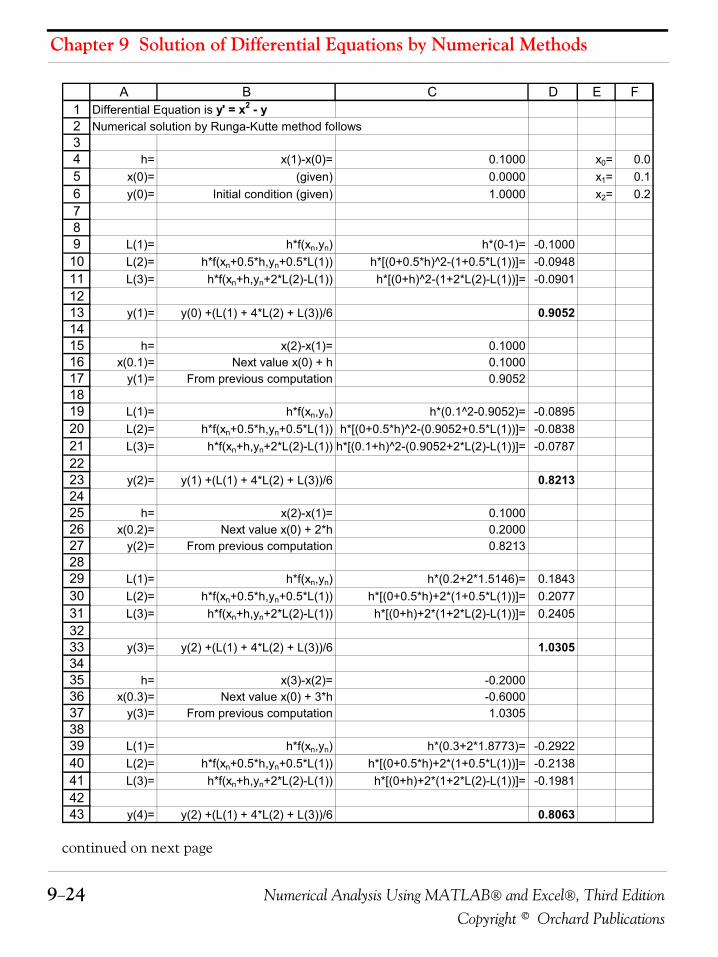
Chapter 9 Solution of Differential Equations by Numerical Methods
9−24 Numerical Analysis Using MATLAB® and Excel®, Third EditionCopyright © Orchard Publications
continued on next page
12345678910111213141516171819202122232425262728293031323334353637383940414243
A B C D E FDifferential Equation is y' = x2 - yNumerical solution by Runga-Kutte method follows
h= x(1)-x(0)= 0.1000 x0= 0.0x(0)= (given) 0.0000 x1= 0.1y(0)= Initial condition (given) 1.0000 x2= 0.2
L(1)= h*f(xn,yn) h*(0-1)= -0.1000L(2)= h*f(xn+0.5*h,yn+0.5*L(1)) h*[(0+0.5*h)^2-(1+0.5*L(1))]= -0.0948L(3)= h*f(xn+h,yn+2*L(2)-L(1)) h*[(0+h)^2-(1+2*L(2)-L(1))]= -0.0901
y(1)= y(0) +(L(1) + 4*L(2) + L(3))/6 0.9052
h= x(2)-x(1)= 0.1000x(0.1)= Next value x(0) + h 0.1000
y(1)= From previous computation 0.9052
L(1)= h*f(xn,yn) h*(0.1^2-0.9052)= -0.0895L(2)= h*f(xn+0.5*h,yn+0.5*L(1)) h*[(0+0.5*h)^2-(0.9052+0.5*L(1))]= -0.0838L(3)= h*f(xn+h,yn+2*L(2)-L(1)) h*[(0.1+h)^2-(0.9052+2*L(2)-L(1))]= -0.0787
y(2)= y(1) +(L(1) + 4*L(2) + L(3))/6 0.8213
h= x(2)-x(1)= 0.1000x(0.2)= Next value x(0) + 2*h 0.2000
y(2)= From previous computation 0.8213
L(1)= h*f(xn,yn) h*(0.2+2*1.5146)= 0.1843L(2)= h*f(xn+0.5*h,yn+0.5*L(1)) h*[(0+0.5*h)+2*(1+0.5*L(1))]= 0.2077L(3)= h*f(xn+h,yn+2*L(2)-L(1)) h*[(0+h)+2*(1+2*L(2)-L(1))]= 0.2405
y(3)= y(2) +(L(1) + 4*L(2) + L(3))/6 1.0305
h= x(3)-x(2)= -0.2000x(0.3)= Next value x(0) + 3*h -0.6000
y(3)= From previous computation 1.0305
L(1)= h*f(xn,yn) h*(0.3+2*1.8773)= -0.2922L(2)= h*f(xn+0.5*h,yn+0.5*L(1)) h*[(0+0.5*h)+2*(1+0.5*L(1))]= -0.2138L(3)= h*f(xn+h,yn+2*L(2)-L(1)) h*[(0+h)+2*(1+2*L(2)-L(1))]= -0.1981
y(4)= y(2) +(L(1) + 4*L(2) + L(3))/6 0.8063
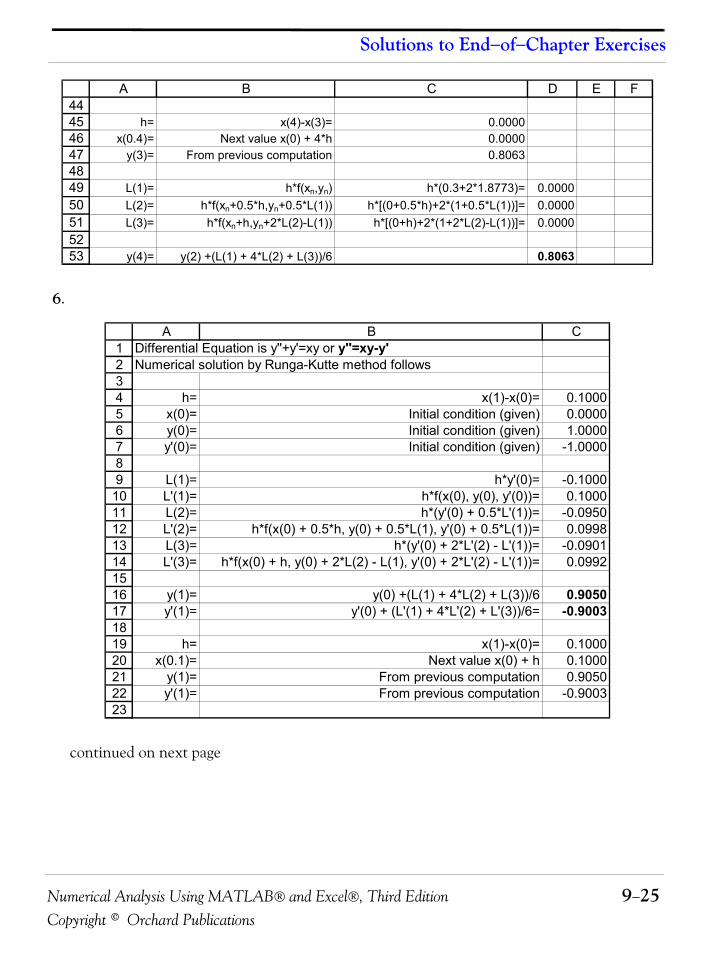
Numerical Analysis Using MATLAB® and Excel®, Third Edition 9−25Copyright © Orchard Publications
Solutions to End−of−Chapter Exercises
6.
continued on next page
44454647484950515253
A B C D E F
h= x(4)-x(3)= 0.0000x(0.4)= Next value x(0) + 4*h 0.0000
y(3)= From previous computation 0.8063
L(1)= h*f(xn,yn) h*(0.3+2*1.8773)= 0.0000L(2)= h*f(xn+0.5*h,yn+0.5*L(1)) h*[(0+0.5*h)+2*(1+0.5*L(1))]= 0.0000L(3)= h*f(xn+h,yn+2*L(2)-L(1)) h*[(0+h)+2*(1+2*L(2)-L(1))]= 0.0000
y(4)= y(2) +(L(1) + 4*L(2) + L(3))/6 0.8063
1234567891011121314151617181920212223
A B CDifferential Equation is y''+y'=xy or y''=xy-y'Numerical solution by Runga-Kutte method follows
h= x(1)-x(0)= 0.1000x(0)= Initial condition (given) 0.0000y(0)= Initial condition (given) 1.0000y'(0)= Initial condition (given) -1.0000
L(1)= h*y'(0)= -0.1000L'(1)= h*f(x(0), y(0), y'(0))= 0.1000L(2)= h*(y'(0) + 0.5*L'(1))= -0.0950L'(2)= h*f(x(0) + 0.5*h, y(0) + 0.5*L(1), y'(0) + 0.5*L(1))= 0.0998L(3)= h*(y'(0) + 2*L'(2) - L'(1))= -0.0901L'(3)= h*f(x(0) + h, y(0) + 2*L(2) - L(1), y'(0) + 2*L'(2) - L'(1))= 0.0992
y(1)= y(0) +(L(1) + 4*L(2) + L(3))/6 0.9050y'(1)= y'(0) + (L'(1) + 4*L'(2) + L'(3))/6= -0.9003
h= x(1)-x(0)= 0.1000x(0.1)= Next value x(0) + h 0.1000
y(1)= From previous computation 0.9050y'(1)= From previous computation -0.9003
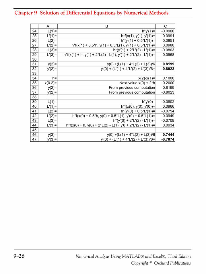
Chapter 9 Solution of Differential Equations by Numerical Methods
9−26 Numerical Analysis Using MATLAB® and Excel®, Third EditionCopyright © Orchard Publications
242526272829303132333435363738394041424344454647
A B CL(1)= h*y'(1)= -0.0900L'(1)= h*f(x(1), y(1), y'(1))= 0.0991L(2)= h*(y'(1) + 0.5*L'(1))= -0.0851L'(2)= h*f(x(1) + 0.5*h, y(1) + 0.5*L(1), y'(1) + 0.5*L'(1))= 0.0980L(3)= h*(y'(1) + 2*L'(2) - L'(1))= -0.0803L'(3)= h*f(x(1) + h, y(1) + 2*L(2) - L(1), y'(1) + 2*L'(2) - L'(1))= 0.0968
y(2)= y(0) +(L(1) + 4*L(2) + L(3))/6 0.8199y'(2)= y'(0) + (L'(1) + 4*L'(2) + L'(3))/6= -0.8023
h= x(2)-x(1)= 0.1000x(0.2)= Next value x(0) + 2*h 0.2000
y(2)= From previous computation 0.8199y'(2)= From previous computation -0.8023
L(1)= h*y'(0)= -0.0802L'(1)= h*f(x(0), y(0), y'(0))= 0.0966L(2)= h*(y'(0) + 0.5*L'(1))= -0.0754L'(2)= h*f(x(0) + 0.5*h, y(0) + 0.5*L(1), y'(0) + 0.5*L(1))= 0.0949L(3)= h*(y'(0) + 2*L'(2) - L'(1))= -0.0709L'(3)= h*f(x(0) + h, y(0) + 2*L(2) - L(1), y'0 + 2*L'(2) - L'(1))= 0.0934
y(3)= y(0) +(L(1) + 4*L(2) + L(3))/6 0.7444y'(3)= y'(0) + (L'(1) + 4*L'(2) + L'(3))/6= -0.7074
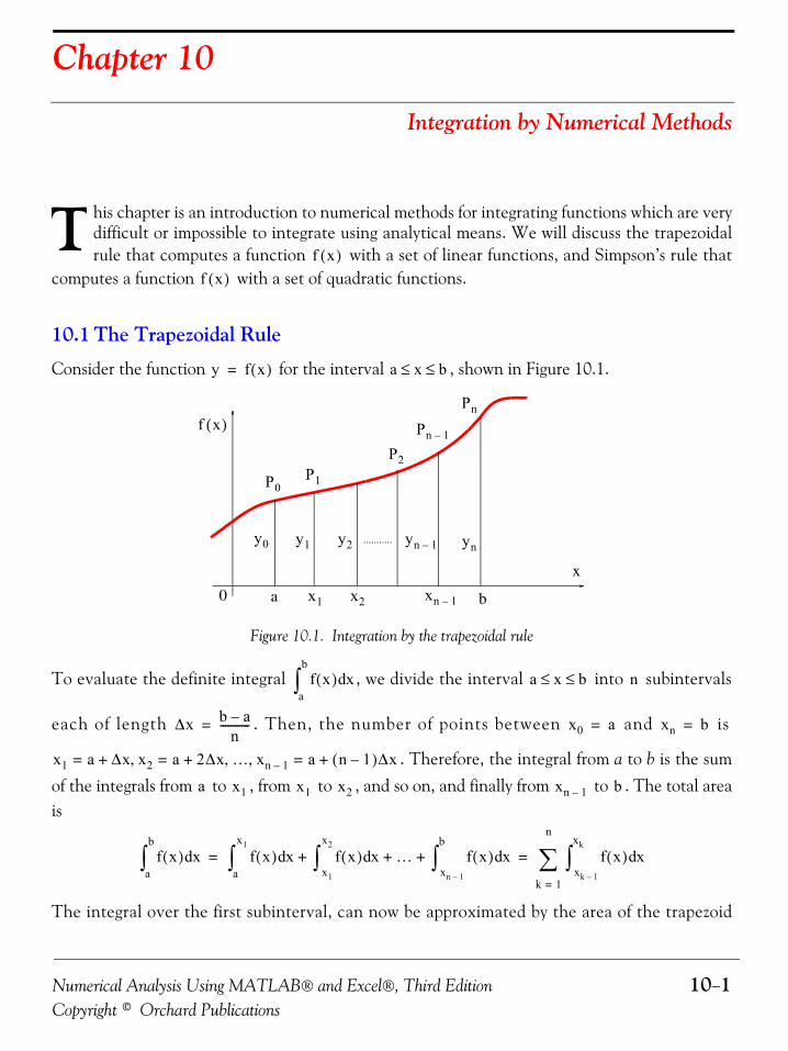
Numerical Analysis Using MATLAB® and Excel®, Third Edition 10−1Copyright © Orchard Publications
Chapter 10
Integration by Numerical Methods
his chapter is an introduction to numerical methods for integrating functions which are verydifficult or impossible to integrate using analytical means. We will discuss the trapezoidalrule that computes a function with a set of linear functions, and Simpson’s rule that
computes a function with a set of quadratic functions.
10.1 The Trapezoidal Rule
Consider the function for the interval , shown in Figure 10.1.
Figure 10.1. Integration by the trapezoidal rule
To evaluate the definite integral , we divide the interval into subintervals
each of length . Then, the number of points between and is
. Therefore, the integral from a to b is the sumof the integrals from to , from to , and so on, and finally from to . The total areais
The integral over the first subinterval, can now be approximated by the area of the trapezoid
T f x( )f x( )
y f x( )= a x b≤ ≤
x
a b
...........
0
f x( )
x1 x2 xn 1–
y0 y1 y2 yn 1– yn
P0P1
P2
Pn 1–
Pn
f x( ) xda
b
∫ a x b≤ ≤ n
Δx b a–n
-----------= x0 a= xn b=
x1 a Δx+= x2 a 2Δx+= … xn 1– a n 1–( )Δx+=, , ,
a x1 x1 x2 xn 1– b
f x( ) xda
b
∫ f x( ) xda
x1
∫ f x( ) xdx1
x2
∫ … f x( ) xdxn 1–
b
∫+ + + f x( ) xdxk 1–
xk
∫k 1=
n
∑= =
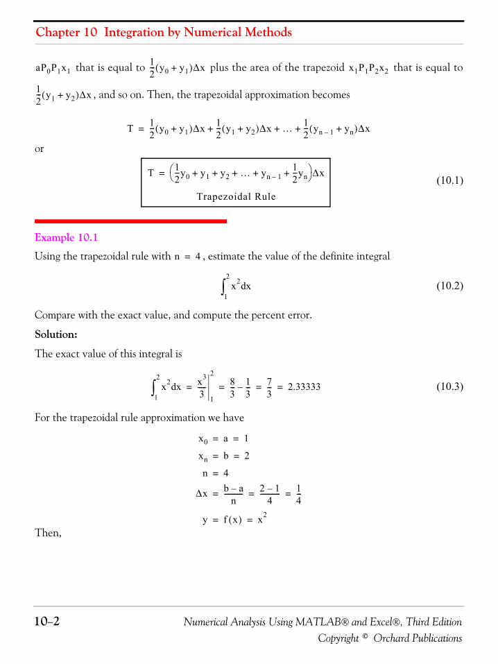
Chapter 10 Integration by Numerical Methods
10−2 Numerical Analysis Using MATLAB® and Excel®, Third EditionCopyright © Orchard Publications
that is equal to plus the area of the trapezoid that is equal to
, and so on. Then, the trapezoidal approximation becomes
or
(10.1)
Example 10.1
Using the trapezoidal rule with , estimate the value of the definite integral
(10.2)
Compare with the exact value, and compute the percent error.
Solution:
The exact value of this integral is
(10.3)
For the trapezoidal rule approximation we have
Then,
aP0P1x112--- y0 y1+( )Δx x1P1P2x2
12--- y1 y2+( )Δx
T 12--- y0 y1+( )Δx 1
2--- y1 y2+( )Δx … 1
2--- yn 1– yn+( )Δx+ + +=
T 12---y0 y1 y2 … yn 1–
12---yn+ + + + +⎝ ⎠
⎛ ⎞Δx=
Trapezoidal Rule
n 4=
x2 xd1
2
∫
x2 xd1
2
∫ x3
3-----
1
283--- 1
3---– 7
3--- 2.33333= = = =
x0 a 1= =
xn b 2= =
n 4=
Δx b a–n
----------- 2 1–4
------------ 14---= = =
y f x( ) x2= =
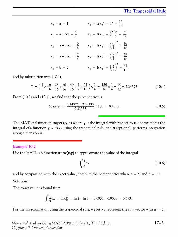
Numerical Analysis Using MATLAB® and Excel®, Third Edition 10−3Copyright © Orchard Publications
The Trapezoidal Rule
and by substitution into (10.1),
(10.4)
From (10.3) and (10.4), we find that the percent error is
(10.5)
The MATLAB function trapz(x,y,n) where y is the integral with respect to x, approximates theintegral of a function using the trapezoidal rule, and n (optional) performs integrationalong dimension .
Example 10.2 Use the MATLAB function trapz(x,y) to approximate the value of the integral
(10.6)
and by comparison with the exact value, compute the percent error when and
Solution:
The exact value is found from
For the approximation using the trapezoidal rule, we let represent the row vector with ,
x0 a 1= = y0 f x0( ) 12 1616------= = =
x1 a Δx+ 54---= = y1 f x1( ) 5
4---⎝ ⎠⎛ ⎞ 2 25
16------= = =
x2 a 2Δx+ 64---= = y2 f x2( ) 6
4---⎝ ⎠
⎛ ⎞ 2 3616------= = =
x3 a 3Δx+ 74---= = y3 f x3( ) 7
4---⎝ ⎠
⎛ ⎞ 2 4916------= = =
x4 b 2= = y4 f x4( ) 84---⎝ ⎠
⎛ ⎞ 2 6416------= = =
T 12--- 16
16------× 25
16------ 36
16------ 49
16------ 1
2--- 64
16------×+ + + +⎝ ⎠
⎛ ⎞ 14---× 150
16--------- 1
4---× 75
32------ 2.34375= == =
% Error 2.34375 2.33333–2.33333
--------------------------------------------- 100× 0.45 %= =
y f x( )=
n
1x--- xd
1
2
∫
n 5= n 10=
1x--- xd
1
2
∫ xln 12 2ln 1ln– 0.6931 0.0000– 0.6931= = = =
x5 n 5=
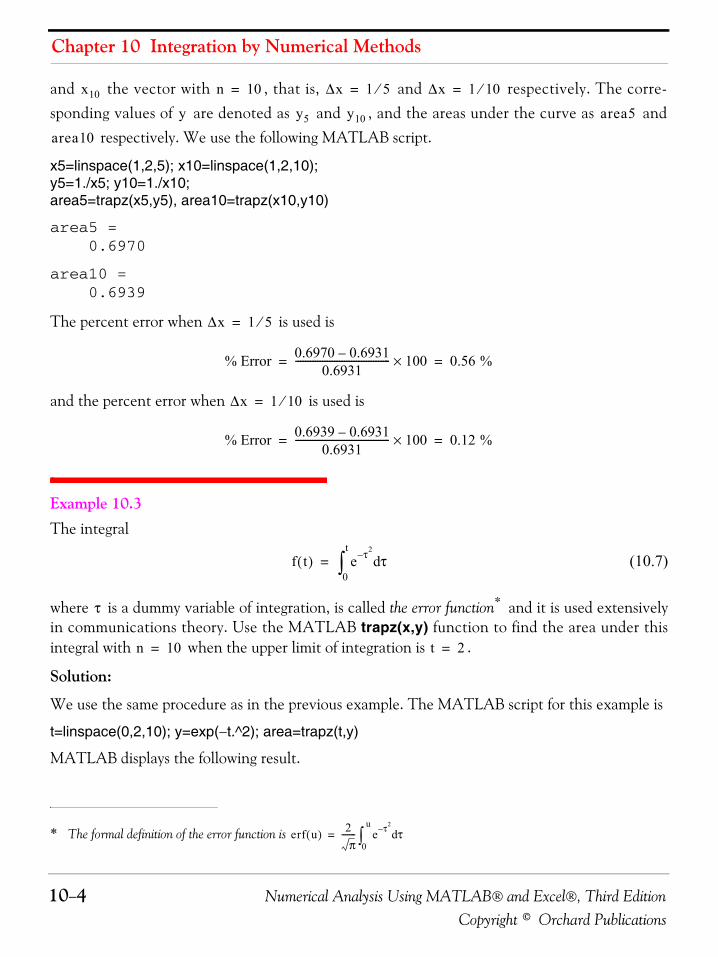
Chapter 10 Integration by Numerical Methods
10−4 Numerical Analysis Using MATLAB® and Excel®, Third EditionCopyright © Orchard Publications
and the vector with , that is, and respectively. The corre-sponding values of are denoted as and , and the areas under the curve as and
respectively. We use the following MATLAB script.
x5=linspace(1,2,5); x10=linspace(1,2,10);y5=1./x5; y10=1./x10;area5=trapz(x5,y5), area10=trapz(x10,y10)
area5 = 0.6970
area10 = 0.6939
The percent error when is used is
and the percent error when is used is
Example 10.3 The integral
(10.7)
where is a dummy variable of integration, is called the error function* and it is used extensivelyin communications theory. Use the MATLAB trapz(x,y) function to find the area under thisintegral with when the upper limit of integration is .
Solution:
We use the same procedure as in the previous example. The MATLAB script for this example is
t=linspace(0,2,10); y=exp(−t.^2); area=trapz(t,y)
MATLAB displays the following result.
* The formal definition of the error function is
x10 n 10= Δx 1 5⁄= Δx 1 10⁄=
y y5 y10 area5
area10
Δx 1 5⁄=
% Error 0.6970 0.6931–0.6931
--------------------------------------- 100× 0.56 %= =
Δx 1 10⁄=
% Error 0.6939 0.6931–0.6931
--------------------------------------- 100× 0.12 %= =
f t( ) e τ2– τd0
t
∫=
τ
erf u( ) 2π
------- e τ2– τd0
u
∫=
n 10= t 2=
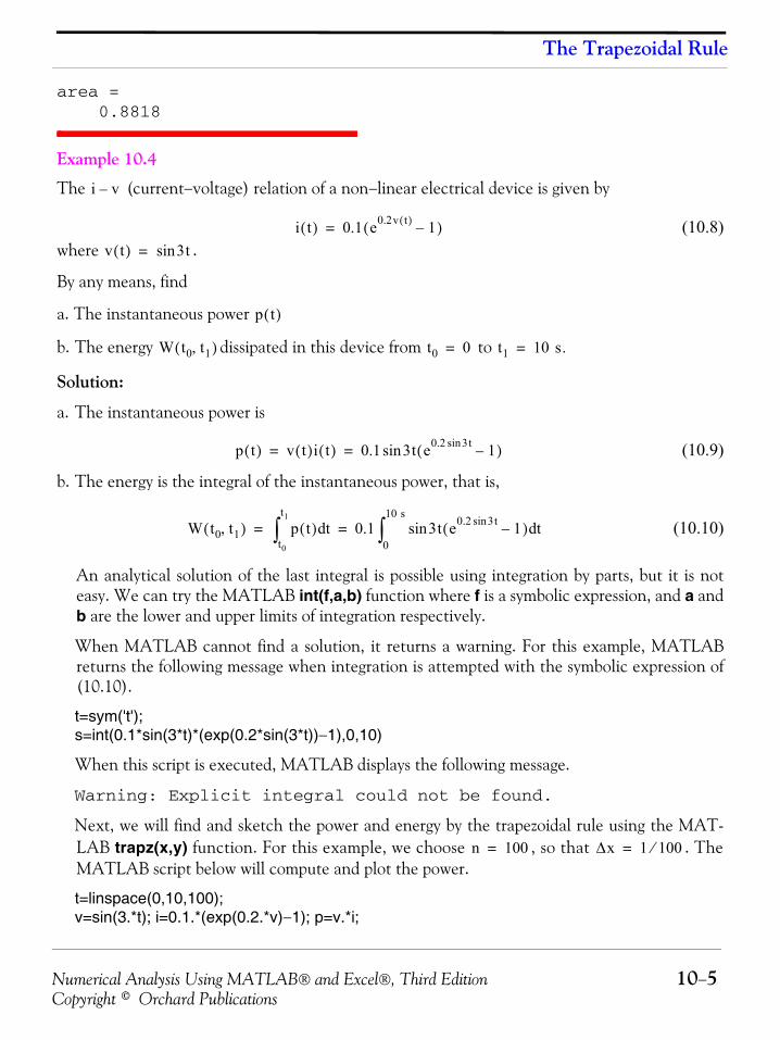
Numerical Analysis Using MATLAB® and Excel®, Third Edition 10−5Copyright © Orchard Publications
The Trapezoidal Rule
area = 0.8818
Example 10.4
The (current−voltage) relation of a non−linear electrical device is given by
(10.8)where .
By any means, find
a. The instantaneous power
b. The energy dissipated in this device from to
Solution:
a. The instantaneous power is
(10.9)
b. The energy is the integral of the instantaneous power, that is,
(10.10)
An analytical solution of the last integral is possible using integration by parts, but it is noteasy. We can try the MATLAB int(f,a,b) function where f is a symbolic expression, and a andb are the lower and upper limits of integration respectively.
When MATLAB cannot find a solution, it returns a warning. For this example, MATLABreturns the following message when integration is attempted with the symbolic expression of(10.10).
t=sym('t');s=int(0.1*sin(3*t)*(exp(0.2*sin(3*t))−1),0,10)
When this script is executed, MATLAB displays the following message.
Warning: Explicit integral could not be found.
Next, we will find and sketch the power and energy by the trapezoidal rule using the MAT-LAB trapz(x,y) function. For this example, we choose , so that . TheMATLAB script below will compute and plot the power.
t=linspace(0,10,100);v=sin(3.*t); i=0.1.*(exp(0.2.*v)−1); p=v.*i;
i v–
i t( ) 0.1 e0.2v t( ) 1–( )=
v t( ) 3tsin=
p t( )
W t0 t1,( ) t0 0= t1 10 s.=
p t( ) v t( )i t( ) 0.1 3t e0.2 3tsin 1–( )sin= =
W t0 t1,( ) p t( ) tdt0
t1
∫ 0.1 3t e0.2 3tsin 1–( ) tdsin0
10 s
∫= =
n 100= Δx 1 100⁄=
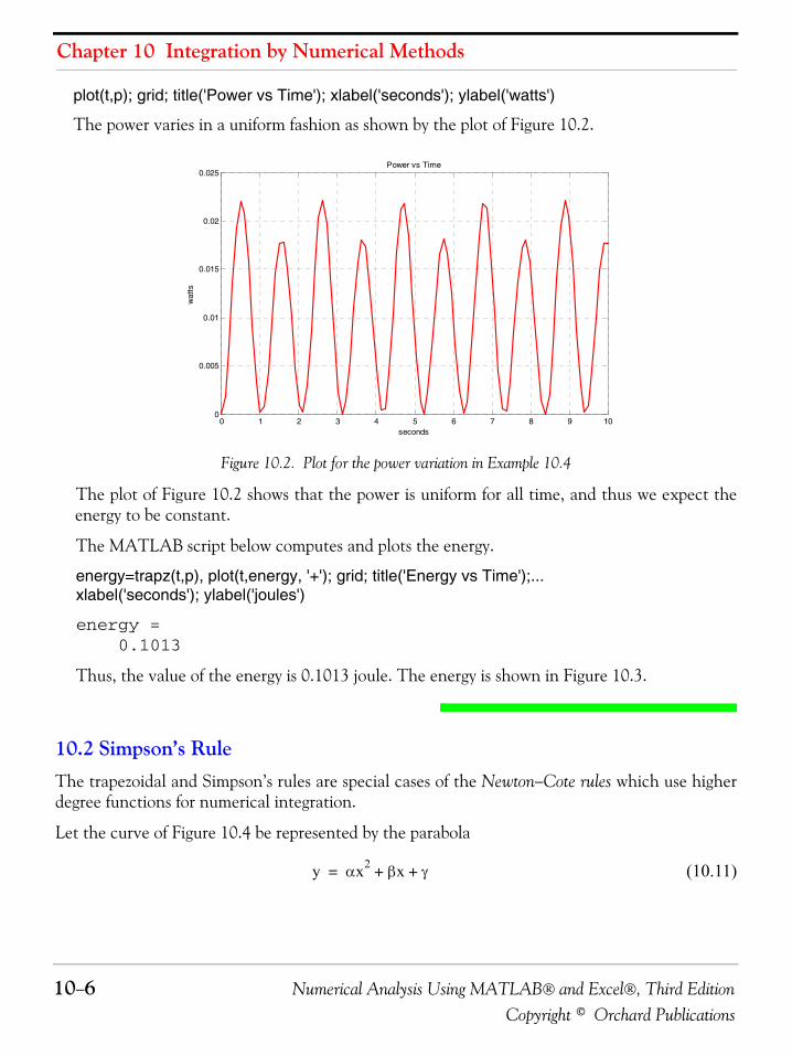
Chapter 10 Integration by Numerical Methods
10−6 Numerical Analysis Using MATLAB® and Excel®, Third EditionCopyright © Orchard Publications
plot(t,p); grid; title('Power vs Time'); xlabel('seconds'); ylabel('watts')
The power varies in a uniform fashion as shown by the plot of Figure 10.2.
Figure 10.2. Plot for the power variation in Example 10.4
The plot of Figure 10.2 shows that the power is uniform for all time, and thus we expect theenergy to be constant.
The MATLAB script below computes and plots the energy.
energy=trapz(t,p), plot(t,energy, '+'); grid; title('Energy vs Time');...xlabel('seconds'); ylabel('joules')
energy = 0.1013
Thus, the value of the energy is 0.1013 joule. The energy is shown in Figure 10.3.
10.2 Simpson’s RuleThe trapezoidal and Simpson’s rules are special cases of the Newton−Cote rules which use higherdegree functions for numerical integration.
Let the curve of Figure 10.4 be represented by the parabola
(10.11)
0 1 2 3 4 5 6 7 8 9 100
0.005
0.01
0.015
0.02
0.025Power vs Time
seconds
wat
ts
y αx2 βx γ+ +=
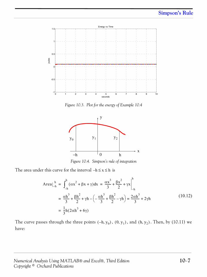
Numerical Analysis Using MATLAB® and Excel®, Third Edition 10−7Copyright © Orchard Publications
Simpson’s Rule
Figure 10.3. Plot for the energy of Example 10.4
Figure 10.4. Simpson’s rule of integration
The area under this curve for the interval is
(10.12)
The curve passes through the three points , , and . Then, by (10.11) wehave:
0 1 2 3 4 5 6 7 8 9 10-1
-0.5
0
0.5
1
1.5Energy vs Time
seconds
joul
es
0x
y
h−h
y2y1y0
h– x h≤ ≤
Area h–h αx2 βx γ+ +( ) xd
h–
h
∫ αx3
3--------- βx2
2-------- γx+ +
h–
h
= =
αh3
3--------- βh2
2-------- γh αh3
3---------– βh2
2-------- γh–+⎝ ⎠
⎛ ⎞–+ + 2αh3
3------------ 2γh+==
13---h 2αh3 6γ+( )=
h– y0,( ) 0 y1,( ) h y2,( )
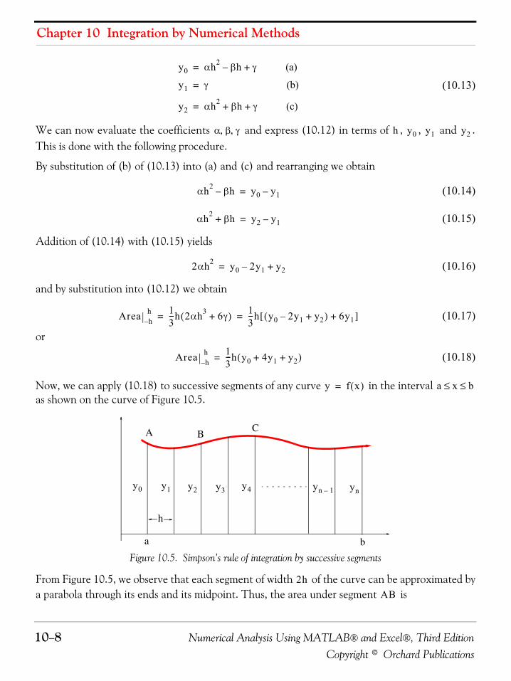
Chapter 10 Integration by Numerical Methods
10−8 Numerical Analysis Using MATLAB® and Excel®, Third EditionCopyright © Orchard Publications
(10.13)
We can now evaluate the coefficients and express (10.12) in terms of , , and .This is done with the following procedure.
By substitution of (b) of (10.13) into (a) and (c) and rearranging we obtain
(10.14)
(10.15)
Addition of (10.14) with (10.15) yields
(10.16)
and by substitution into (10.12) we obtain
(10.17)
or
(10.18)
Now, we can apply (10.18) to successive segments of any curve in the interval as shown on the curve of Figure 10.5.
Figure 10.5. Simpson’s rule of integration by successive segments
From Figure 10.5, we observe that each segment of width of the curve can be approximated bya parabola through its ends and its midpoint. Thus, the area under segment is
y0 αh2 βh– γ (a)+=
y1 γ (b)=
y2 αh2 βh γ (c)+ +=
α β γ, , h y0 y1 y2
αh2 βh– y0 y1–=
αh2 βh+ y2 y1–=
2αh2 y0 2y1– y2+=
Area h–h 1
3---h 2αh3 6γ+( ) 1
3---h y0 2y1– y2+( ) 6y1+[ ]= =
Area h–h 1
3---h y0 4y1 y2+ +( )=
y f x( )= a x b≤ ≤
a b
h
A BC
yn 1–y4y3y2y1y0 yn
2hAB
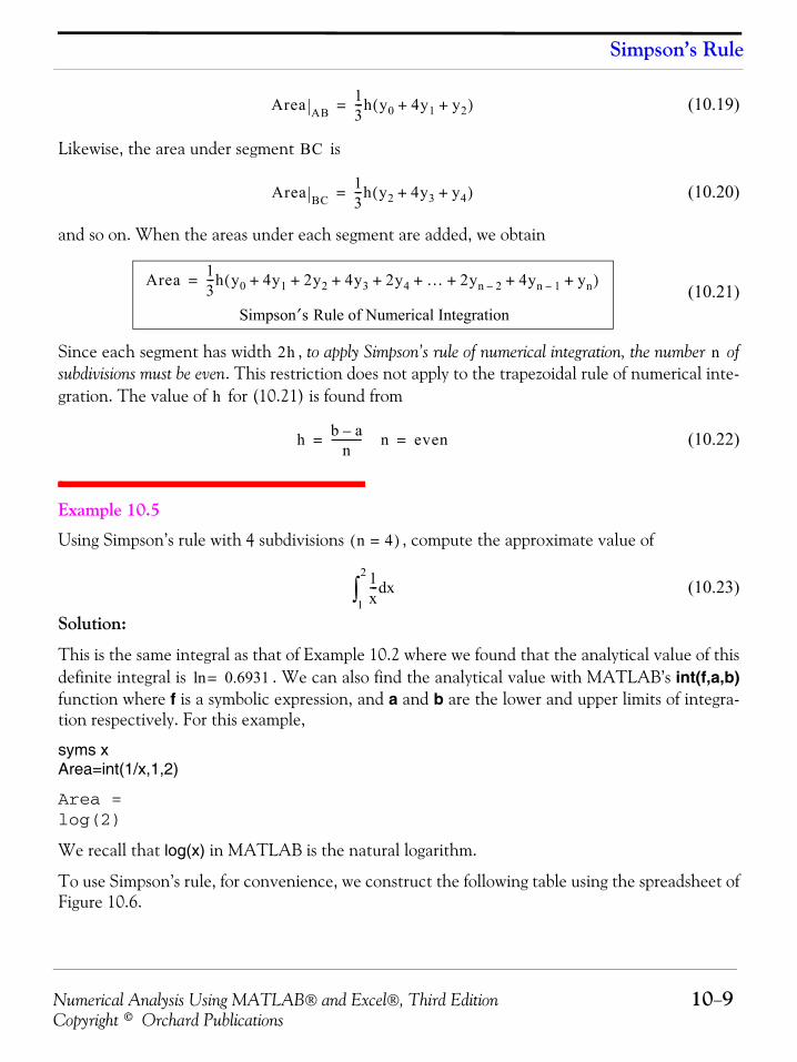
Numerical Analysis Using MATLAB® and Excel®, Third Edition 10−9Copyright © Orchard Publications
Simpson’s Rule
(10.19)
Likewise, the area under segment is
(10.20)
and so on. When the areas under each segment are added, we obtain
(10.21)
Since each segment has width , to apply Simpson’s rule of numerical integration, the number ofsubdivisions must be even. This restriction does not apply to the trapezoidal rule of numerical inte-gration. The value of for (10.21) is found from
(10.22)
Example 10.5
Using Simpson’s rule with 4 subdivisions , compute the approximate value of
(10.23)
Solution:
This is the same integral as that of Example 10.2 where we found that the analytical value of thisdefinite integral is . We can also find the analytical value with MATLAB’s int(f,a,b)function where f is a symbolic expression, and a and b are the lower and upper limits of integra-tion respectively. For this example,
syms xArea=int(1/x,1,2)
Area =log(2)
We recall that log(x) in MATLAB is the natural logarithm.
To use Simpson’s rule, for convenience, we construct the following table using the spreadsheet ofFigure 10.6.
Area AB13---h y0 4y1 y2+ +( )=
BC
Area BC13---h y2 4y3 y4+ +( )=
Area 13---h y0 4y1 2y2+ + 4y3 2y4 … 2yn 2– 4yn 1– yn+ + + + + +( )=
Simpson′s Rule of Numerical Integration
2h n
h
h b a–n
----------- n even= =
n 4=( )
1x--- xd
1
2
∫
0.6931=ln
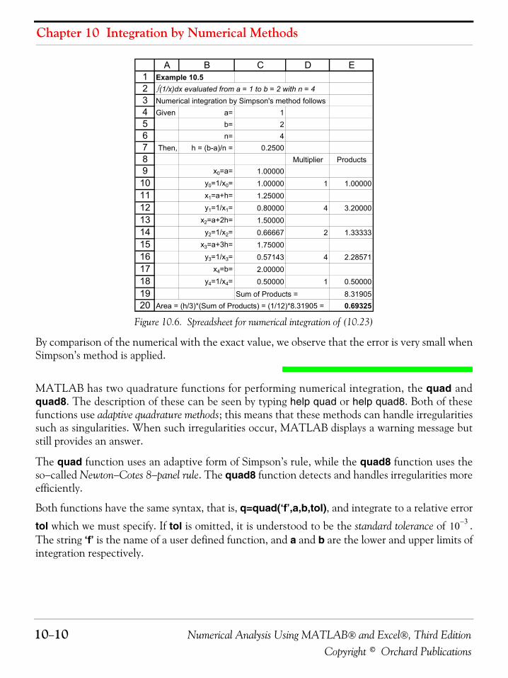
Chapter 10 Integration by Numerical Methods
10−10 Numerical Analysis Using MATLAB® and Excel®, Third EditionCopyright © Orchard Publications
Figure 10.6. Spreadsheet for numerical integration of (10.23)
By comparison of the numerical with the exact value, we observe that the error is very small whenSimpson’s method is applied.
MATLAB has two quadrature functions for performing numerical integration, the quad andquad8. The description of these can be seen by typing help quad or help quad8. Both of thesefunctions use adaptive quadrature methods; this means that these methods can handle irregularitiessuch as singularities. When such irregularities occur, MATLAB displays a warning message butstill provides an answer.
The quad function uses an adaptive form of Simpson’s rule, while the quad8 function uses theso−called Newton−Cotes 8−panel rule. The quad8 function detects and handles irregularities moreefficiently.
Both functions have the same syntax, that is, q=quad(‘f’,a,b,tol), and integrate to a relative error
tol which we must specify. If tol is omitted, it is understood to be the standard tolerance of .The string ‘f’ is the name of a user defined function, and a and b are the lower and upper limits ofintegration respectively.
123456789
1011121314151617181920
A B C D EExample 10.5∫ (1/x)dx evaluated from a = 1 to b = 2 with n = 4Numerical integration by Simpson's method followsGiven a= 1
b= 2n= 4
Then, h = (b-a)/n = 0.2500Multiplier Products
x0=a= 1.00000y0=1/x0= 1.00000 1 1.00000x1=a+h= 1.25000y1=1/x1= 0.80000 4 3.20000
x2=a+2h= 1.50000y2=1/x2= 0.66667 2 1.33333
x3=a+3h= 1.75000y3=1/x3= 0.57143 4 2.28571
x4=b= 2.00000y4=1/x4= 0.50000 1 0.50000
Sum of Products = 8.31905Area = (h/3)*(Sum of Products) = (1/12)*8.31905 = 0.69325
10 3–
Numerical Analysis Using MATLAB® and Excel®, Third Edition 10−11Copyright © Orchard Publications
Simpson’s Rule
Example 10.6 Given the definite integral
(10.24)
a. Use MATLAB’s symbolic int function to obtain the value of this integral
b. Obtain the value of this integral with the q=quad(‘f’,a,b) function
c. Obtain the value of this integral with the q=quad(‘f’,a,b,tol) function where
d. Obtain the value of this integral with the q=quad8(‘f’,a,b) function
e. Obtain the value of this integral with the q=quad8(‘f’,a,b,tol) function where
Solution:
a.syms x; y=int(exp(−x^2),0,2) % Define symbolic variable x and integrate
y =1/2*erf(2)*pi^(1/2)pretty(y)
1/2 1/2 erf(2) pi
erf is an acronym for the error function and we can obtain its definition with help erf
b. First, we need to create and save a function m−file. We name it errorfcn1.m as shown below.We will use format long to display the values with 15 digits.
function y = errorfcn1(x)y = exp(−x.^2);
With this file saved as errorfcn1.m, we write and execute the following MATLAB script.
format longy_std=quad('errorfcn1',0,2)
We obtain the answer in standard tolerance form as
y_std = 0.88211275610253
c. With the specified tolerance, the script and the answer are as follows:
y_tol=quad('errorfcn1',0,2,10^−10)
y_tol = 0.88208139076242
y f x( )= e x2– xd0
2
∫=
tol 10 10–=
tol 10 10–=
Chapter 10 Integration by Numerical Methods
10−12 Numerical Analysis Using MATLAB® and Excel®, Third EditionCopyright © Orchard Publications
d. With the standard tolerance,
y_std8=quad8('errorfcn1',0,2)
y_std8 = 0.88208139076194
e. With the specified tolerance,
y_tol8=quad8('errorfcn1',0,2,10^−10)
y_tol8 = 0.88208139076242
We observe that with the tolerance, both quad and quad8 produce the same result.
Example 10.7 Using the quad and quad8 functions with standard tolerance, evaluate the integral
(10.25)
at and . Use the fprintf function to display first the analyticalvalues, then, the numerical values produced by the quad and quad8 functions for each set ofdata.
Solution:
Evaluating the given integral, we obtain
(10.26)
where and are non−negative values. Substitution of the values of the given values of and will be included in the MATLAB script below.
The sqrt function in a built−in function and therefore, we need not write a user defined m−file.We will include the input function in the script. The script is then saved as Example_10_7.
% This script displays the approximations obtained with the quad and quad8 functions% with the analytical results for the integration of the square root of x over the % interval (a,b) where a and b are non−negative.% fprintf(' \n'); % Insert linea=input('Enter first point "a" (non−negative): ');b=input('Enter second point "b" (non−negative): ');
10 10–
y f x( ) x xda
b
∫= =
a b,( ) 0.2 0.8,( ) 1.4 2.3,( ),=( ), (3,8)
y x1 2⁄ xda
b
∫ x3 2⁄
3 2⁄----------
a
b23--- b3 2⁄ a3 2⁄–( )= = =
a b a b
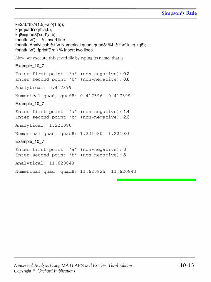
Numerical Analysis Using MATLAB® and Excel®, Third Edition 10−13Copyright © Orchard Publications
Simpson’s Rule
k=2/3.*(b.^(1.5)−a.^(1.5));kq=quad('sqrt',a,b);kq8=quad8('sqrt',a,b);fprintf(' \n');... % Insert linefprintf(' Analytical: %f \n Numerical quad, quad8: %f %f \n',k,kq,kq8);...fprintf(' \n'); fprintf(' \n') % Insert two lines
Now, we execute this saved file by typing its name, that is,
Example_10_7
Enter first point "a" (non-negative): 0.2Enter second point "b" (non-negative): 0.8
Analytical: 0.417399
Numerical quad, quad8: 0.417396 0.417399
Example_10_7
Enter first point "a" (non-negative): 1.4Enter second point "b" (non-negative): 2.3
Analytical: 1.221080
Numerical quad, quad8: 1.221080 1.221080
Example_10_7
Enter first point "a" (non-negative): 3Enter second point "b" (non-negative): 8
Analytical: 11.620843
Numerical quad, quad8: 11.620825 11.620843
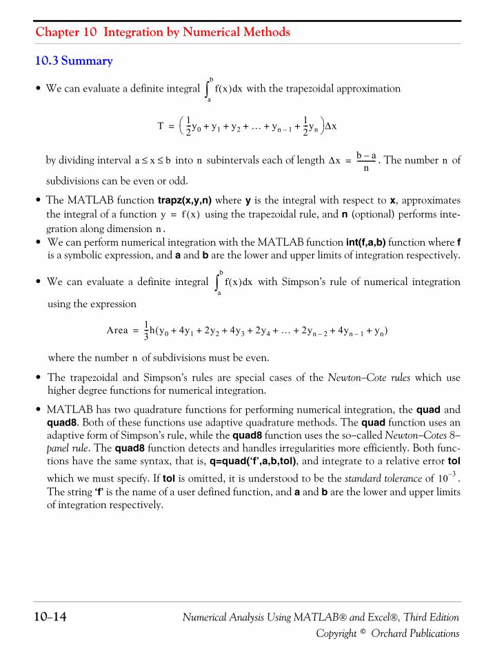
Chapter 10 Integration by Numerical Methods
10−14 Numerical Analysis Using MATLAB® and Excel®, Third EditionCopyright © Orchard Publications
10.3 Summary
• We can evaluate a definite integral with the trapezoidal approximation
by dividing interval into subintervals each of length . The number of
subdivisions can be even or odd.
• The MATLAB function trapz(x,y,n) where y is the integral with respect to x, approximatesthe integral of a function using the trapezoidal rule, and n (optional) performs inte-gration along dimension .
• We can perform numerical integration with the MATLAB function int(f,a,b) function where fis a symbolic expression, and a and b are the lower and upper limits of integration respectively.
• We can evaluate a definite integral with Simpson’s rule of numerical integration
using the expression
where the number of subdivisions must be even.
• The trapezoidal and Simpson’s rules are special cases of the Newton−Cote rules which usehigher degree functions for numerical integration.
• MATLAB has two quadrature functions for performing numerical integration, the quad andquad8. Both of these functions use adaptive quadrature methods. The quad function uses anadaptive form of Simpson’s rule, while the quad8 function uses the so−called Newton−Cotes 8−panel rule. The quad8 function detects and handles irregularities more efficiently. Both func-tions have the same syntax, that is, q=quad(‘f’,a,b,tol), and integrate to a relative error tol
which we must specify. If tol is omitted, it is understood to be the standard tolerance of .The string ‘f’ is the name of a user defined function, and a and b are the lower and upper limitsof integration respectively.
f x( ) xda
b
∫
T 12---y0 y1 y2 … yn 1–
12---yn+ + + + +⎝ ⎠
⎛ ⎞Δx=
a x b≤ ≤ n Δx b a–n
-----------= n
y f x( )=
n
f x( ) xda
b
∫
Area 13---h y0 4y1 2y2+ + 4y3 2y4 … 2yn 2– 4yn 1– yn+ + + + + +( )=
n
10 3–
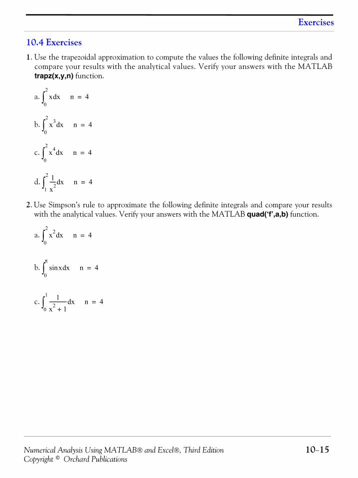
Numerical Analysis Using MATLAB® and Excel®, Third Edition 10−15Copyright © Orchard Publications
Exercises
10.4 Exercises1. Use the trapezoidal approximation to compute the values the following definite integrals and
compare your results with the analytical values. Verify your answers with the MATLABtrapz(x,y,n) function.
a.
b.
c.
d.
2. Use Simpson’s rule to approximate the following definite integrals and compare your resultswith the analytical values. Verify your answers with the MATLAB quad(‘f’,a,b) function.
a.
b.
c.
x xd0
2
∫ n 4=
x3 xd0
2
∫ n 4=
x4 xd0
2
∫ n 4=
1x2----- xd
1
2
∫ n 4=
x2 xd0
2
∫ n 4=
x xdsin0
π
∫ n 4=
1x2 1+-------------- xd
0
1
∫ n 4=
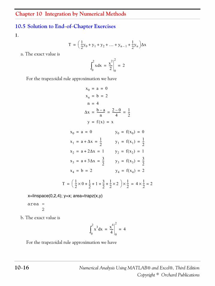
Chapter 10 Integration by Numerical Methods
10−16 Numerical Analysis Using MATLAB® and Excel®, Third EditionCopyright © Orchard Publications
10.5 Solution to End−of−Chapter Exercises1.
a. The exact value is
For the trapezoidal rule approximation we have
x=linspace(0,2,4); y=x; area=trapz(x,y)
area = 2
b. The exact value is
For the trapezoidal rule approximation we have
T 12---y0 y1 y2 … yn 1–
12---yn+ + + + +⎝ ⎠
⎛ ⎞Δx=
x xd0
2
∫ x2
2-----
0
2
2= =
x0 a 0= =
xn b 2= =
n 4=
Δx b a–n
----------- 2 0–4
------------ 12---= = =
y f x( ) x= =
x0 a 0= = y0 f x0( ) 0= =
x1 a Δx+ 12---= = y1 f x1( ) 1
2---= =
x2 a 2Δx+ 1= = y2 f x2( ) 1= =
x3 a 3Δx+ 32---= = y3 f x3( ) 3
2---= =
x4 b 2= = y4 f x4( ) 2= =
T 12--- 0× 1
2--- 1 3
2--- 1
2--- 2×+ + + +⎝ ⎠
⎛ ⎞ 12---× 4 1
2---× 2== =
x3 xd0
2
∫ x4
4-----
0
2
4= =
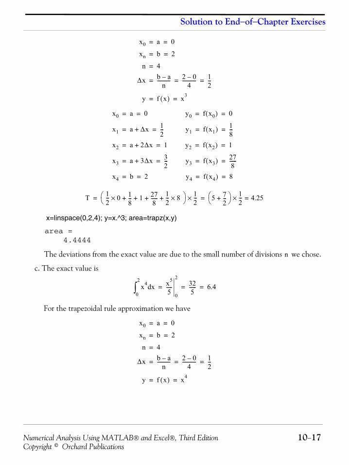
Numerical Analysis Using MATLAB® and Excel®, Third Edition 10−17Copyright © Orchard Publications
Solution to End−of−Chapter Exercises
x=linspace(0,2,4); y=x.^3; area=trapz(x,y)
area = 4.4444
The deviations from the exact value are due to the small number of divisions we chose.
c. The exact value is
For the trapezoidal rule approximation we have
x0 a 0= =
xn b 2= =
n 4=
Δx b a–n
----------- 2 0–4
------------ 12---= = =
y f x( ) x3= =
x0 a 0= = y0 f x0( ) 0= =
x1 a Δx+ 12---= = y1 f x1( ) 1
8---= =
x2 a 2Δx+ 1= = y2 f x2( ) 1= =
x3 a 3Δx+ 32---= = y3 f x3( ) 27
8------= =
x4 b 2= = y4 f x4( ) 8= =
T 12--- 0× 1
8--- 1 27
8------ 1
2--- 8×+ + + +⎝ ⎠
⎛ ⎞ 12---× 5 7
2---+⎝ ⎠
⎛ ⎞ 12---× 4.25== =
n
x4 xd0
2
∫ x5
5-----
0
2325
------ 6.4= = =
x0 a 0= =
xn b 2= =
n 4=
Δx b a–n
----------- 2 0–4
------------ 12---= = =
y f x( ) x4= =
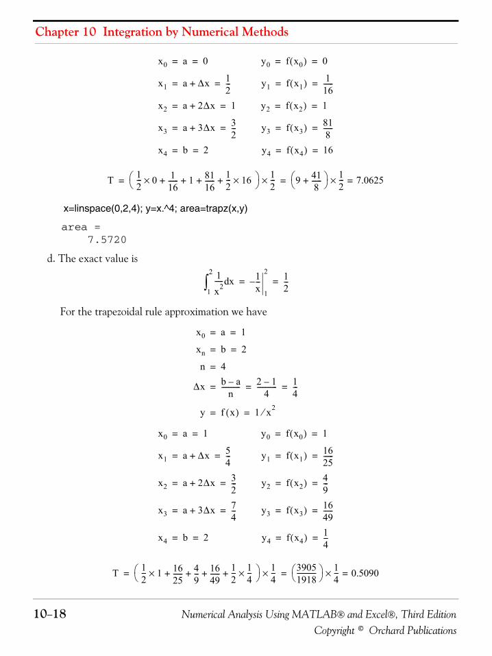
Chapter 10 Integration by Numerical Methods
10−18 Numerical Analysis Using MATLAB® and Excel®, Third EditionCopyright © Orchard Publications
x=linspace(0,2,4); y=x.^4; area=trapz(x,y)
area = 7.5720
d. The exact value is
For the trapezoidal rule approximation we have
x0 a 0= = y0 f x0( ) 0= =
x1 a Δx+ 12---= = y1 f x1( ) 1
16------= =
x2 a 2Δx+ 1= = y2 f x2( ) 1= =
x3 a 3Δx+ 32---= = y3 f x3( ) 81
8------= =
x4 b 2= = y4 f x4( ) 16= =
T 12--- 0× 1
16------ 1 81
16------ 1
2--- 16×+ + + +⎝ ⎠
⎛ ⎞ 12---× 9 41
8------+⎝ ⎠
⎛ ⎞ 12---× 7.0625== =
1x2----- xd
1
2
∫ 1x---–
1
2 12---= =
x0 a 1= =
xn b 2= =
n 4=
Δx b a–n
----------- 2 1–4
------------ 14---= = =
y f x( ) 1 x2⁄= =
x0 a 1= = y0 f x0( ) 1= =
x1 a Δx+ 54---= = y1 f x1( ) 16
25------= =
x2 a 2Δx+ 32---= = y2 f x2( ) 4
9---= =
x3 a 3Δx+ 74---= = y3 f x3( ) 16
49------= =
x4 b 2= = y4 f x4( ) 14---= =
T 12--- 1× 16
25------ 4
9--- 16
49------ 1
2--- 1
4---×+ + + +⎝ ⎠
⎛ ⎞ 14---× 3905
1918------------⎝ ⎠⎛ ⎞ 1
4---× 0.5090== =
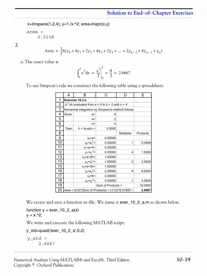
Numerical Analysis Using MATLAB® and Excel®, Third Edition 10−19Copyright © Orchard Publications
Solution to End−of−Chapter Exercises
x=linspace(1,2,4); y=1./x.^2; area=trapz(x,y)
area = 0.5158
2.
a. The exact value is
To use Simpson’s rule we construct the following table using a spreadsheet.
We create and save a function m−file. We name it exer_10_2_a.m as shown below.
function y = exer_10_2_a(x)y = x.^2;
We write and execute the following MATLAB script:
y_std=quad('exer_10_2_a',0,2)
y_std = 2.6667
Area 13---h y0 4y1 2y2+ + 4y3 2y4 … 2yn 2– 4yn 1– yn+ + + + + +( )=
x2 xd0
2
∫ x3
3-----
0
283--- 2.6667= = =
1234567891011121314151617181920
A B C D EExercise 10.2.a∫ x 2 dx evaluated from a = 0 to b = 2 with n = 4Numerical integration by Simpson's method followsGiven a= 0
b= 2n= 4
Then, h = (b-a)/n = 0.5000Multiplier Products
x0=a= 0.00000y0=x0
2= 0.00000 1 0.0000x1=a+h= 0.50000y1=x1
2= 0.25000 4 1.0000x2=a+2h= 1.00000
y2=x22= 1.00000 2 2.0000
x3=a+3h= 1.50000y3=x3
2= 2.25000 4 9.0000x4=b= 2.00000
y4=x42= 4.00000 1 4.0000
Sum of Products = 16.0000Area = (h/3)*(Sum of Products) = (1/12)*8.31905 = 2.6667
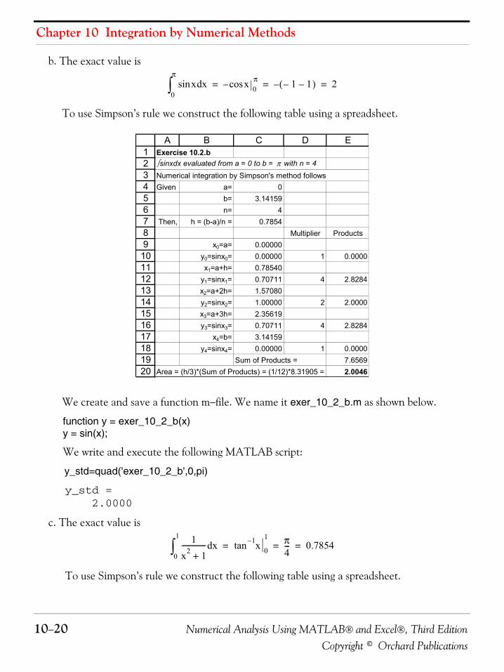
Chapter 10 Integration by Numerical Methods
10−20 Numerical Analysis Using MATLAB® and Excel®, Third EditionCopyright © Orchard Publications
b. The exact value is
To use Simpson’s rule we construct the following table using a spreadsheet.
We create and save a function m−file. We name it exer_10_2_b.m as shown below.
function y = exer_10_2_b(x)y = sin(x);
We write and execute the following MATLAB script:
y_std=quad('exer_10_2_b',0,pi)
y_std = 2.0000
c. The exact value is
To use Simpson’s rule we construct the following table using a spreadsheet.
x xdsin0
π
∫ xcos– 0π 1– 1–( )– 2= = =
1234567891011121314151617181920
A B C D EExercise 10.2.b∫ sinxdx evaluated from a = 0 to b = π with n = 4Numerical integration by Simpson's method followsGiven a= 0
b= 3.14159n= 4
Then, h = (b-a)/n = 0.7854Multiplier Products
x0=a= 0.00000y0=sinx0= 0.00000 1 0.0000x1=a+h= 0.78540
y1=sinx1= 0.70711 4 2.8284x2=a+2h= 1.57080y2=sinx2= 1.00000 2 2.0000x3=a+3h= 2.35619y3=sinx3= 0.70711 4 2.8284
x4=b= 3.14159y4=sinx4= 0.00000 1 0.0000
Sum of Products = 7.6569Area = (h/3)*(Sum of Products) = (1/12)*8.31905 = 2.0046
1x2 1+-------------- xd
0
1
∫ x1–tan 0
1 π4--- 0.7854= = =
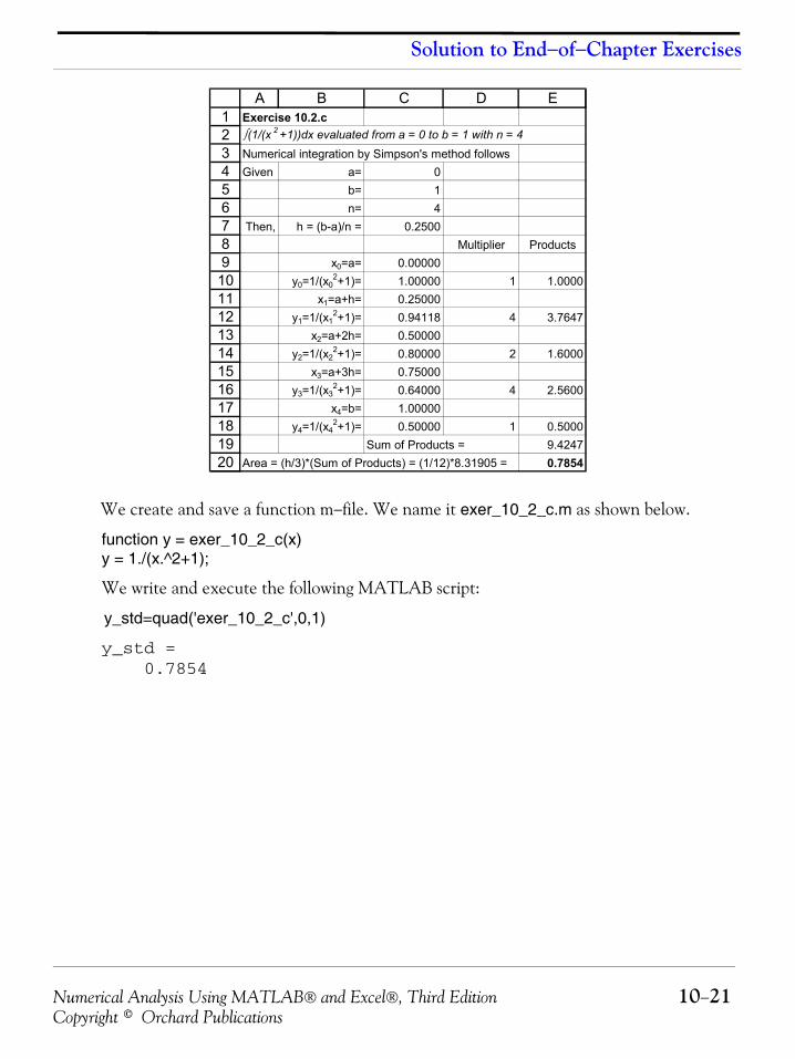
Numerical Analysis Using MATLAB® and Excel®, Third Edition 10−21Copyright © Orchard Publications
Solution to End−of−Chapter Exercises
We create and save a function m−file. We name it exer_10_2_c.m as shown below.
function y = exer_10_2_c(x)y = 1./(x.^2+1);
We write and execute the following MATLAB script:
y_std=quad('exer_10_2_c',0,1)
y_std = 0.7854
1234567891011121314151617181920
A B C D EExercise 10.2.c∫ (1/(x 2 +1))dx evaluated from a = 0 to b = 1 with n = 4Numerical integration by Simpson's method followsGiven a= 0
b= 1n= 4
Then, h = (b-a)/n = 0.2500Multiplier Products
x0=a= 0.00000y0=1/(x0
2+1)= 1.00000 1 1.0000x1=a+h= 0.25000
y1=1/(x12+1)= 0.94118 4 3.7647
x2=a+2h= 0.50000y2=1/(x2
2+1)= 0.80000 2 1.6000x3=a+3h= 0.75000
y3=1/(x32+1)= 0.64000 4 2.5600x4=b= 1.00000
y4=1/(x42+1)= 0.50000 1 0.5000
Sum of Products = 9.4247Area = (h/3)*(Sum of Products) = (1/12)*8.31905 = 0.7854
Numerical Analysis Using MATLAB® and Excel®, Third Edition 11−1Copyright © Orchard Publications
Chapter 11
Difference Equations
his chapter is an introduction to difference equations based on finite differences. The dis-cussion is limited to linear difference equations with constant coefficients. The Fibonaccinumbers are defined, and a practical example in electric circuit theory is given at the end
of this chapter.
11.1 Introduction
In mathematics, a recurrence relation is an equation which defines a sequence recursively: eachterm of the sequence is defined as a function of the preceding terms. A difference equation is aspecific type of recurrence relation, and this type is discussed in this chapter. Difference equa-tions as used with discrete type systems, are discussed in Appendix A.
11.2 Definition, Solutions, and ApplicationsThe difference equations discussed in this chapter, are used in numerous applications such asengineering, mathematics, physics, and other sciences.
The general form of a linear, constant coefficient difference equation has the form
(11.1)
where represents a constant coefficient and is an operator similar to the operator inordinary differential equations. The operator increases the argument of a function by oneinterval , and is a positive integer that denotes the order of the difference equation.
In terms of the interval , the difference operator is
(11.2)
The interval is usually unity, i.e., , and the subscript is normally omitted. Thus,(11.2) is written as
(11.3)
If, in (11.3), we increase the argument of by another unit, we obtain the second order operator
, that is,
T
arEr ar 1– E r 1– …+ + a1E a0+ +( )y φ x( )=
ak E D
Eh r
h E
Ef xk( ) f xk h+( ) f xk h+( )= =
h h 1= k
Ef x( ) f x 1+( ) fx 1+= =
f
E 2
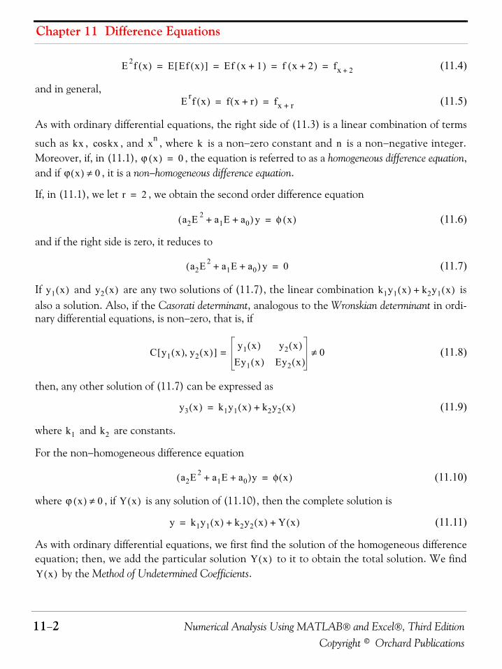
Chapter 11 Difference Equations
11−2 Numerical Analysis Using MATLAB® and Excel®, Third EditionCopyright © Orchard Publications
(11.4)
and in general,(11.5)
As with ordinary differential equations, the right side of (11.3) is a linear combination of terms
such as , , and , where is a non−zero constant and is a non−negative integer.Moreover, if, in (11.1), , the equation is referred to as a homogeneous difference equation,and if , it is a non−homogeneous difference equation.
If, in (11.1), we let , we obtain the second order difference equation
(11.6)
and if the right side is zero, it reduces to
(11.7)
If and are any two solutions of (11.7), the linear combination isalso a solution. Also, if the Casorati determinant, analogous to the Wronskian determinant in ordi-nary differential equations, is non−zero, that is, if
(11.8)
then, any other solution of (11.7) can be expressed as
(11.9)
where and are constants.
For the non−homogeneous difference equation
(11.10)
where , if is any solution of (11.10), then the complete solution is
(11.11)
As with ordinary differential equations, we first find the solution of the homogeneous differenceequation; then, we add the particular solution to it to obtain the total solution. We find
by the Method of Undetermined Coefficients.
E 2f x( ) E Ef x( )[ ] Ef x 1+( ) f x 2+( ) fx 2+= = = =
E rf x( ) f x r+( ) fx r+= =
kx kxcos xn k nϕ x( ) 0=
ϕ x( ) 0≠
r 2=
a2E 2 a1E a0+ +( )y φ x( )=
a2E 2 a1E a0+ +( )y 0=
y1 x( ) y2 x( ) k1y1 x( ) k2y1 x( )+
C y1 x( ) y2 x( ),[ ]y1 x( ) y2 x( )
Ey1 x( ) Ey2 x( )= 0≠
y3 x( ) k1y1 x( ) k2y2 x( )+=
k1 k2
a2E 2 a1E a0+ +( )y φ x( )=
ϕ x( ) 0≠ Y x( )
y k1y1 x( ) k2y2 x( ) Y x( )+ +=
Y x( )Y x( )
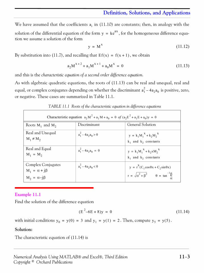
Numerical Analysis Using MATLAB® and Excel®, Third Edition 11−3Copyright © Orchard Publications
Definition, Solutions, and Applications
We have assumed that the coefficients in (11.10) are constants; then, in analogy with the
solution of the differential equation of the form , for the homogeneous difference equa-tion we assume a solution of the form
(11.12)
By substitution into (11.7), and recalling that , we obtain
(11.13)
and this is the characteristic equation of a second order difference equation.
As with algebraic quadratic equations, the roots of (11.13) can be real and unequal, real and
equal, or complex conjugates depending on whether the discriminant is positive, zero,or negative. These cases are summarized in Table 11.1.
Example 11.1 Find the solution of the difference equation
(11.14)
with initial conditions and . Then, compute .
Solution:
The characteristic equation of (11.14) is
TABLE 11.1 Roots of the characteristic equation in difference equations
Characteristic equation of
Roots and Discriminant General Solution
Real and Unequal
Real and Equal
Complex Conjugates
ai
y keax=
y M x=
Ef x( ) f x 1+( )=
a2M x 2+ a1M x 1+ a0M x+ + 0=
a12 4a2a0–
a2 M 2 a1 M a0+ + 0= a2E 2 a1E a0+ +( )y 0=
M1 M2
M1 M2≠a1
2 4a2a0– 0> y k1M1x k2M2
x+=
k1 and k2 cons tstan
M1 M2=a1
2 4a2a0– 0= y k1M1x k2xM2
x+=
k1 and k2 cons tstan
M1 α jβ+=
M2 α j– β=
a12 4a2a0 0<– y rx C1 θx C2 θxsin+cos( )=
r α2 β2+= θ βα---
1–tan=
E 2 6– E 8+( )y 0=
y0 y 0( ) 3= = y1 y 1( ) 2= = y5 y 5( )=
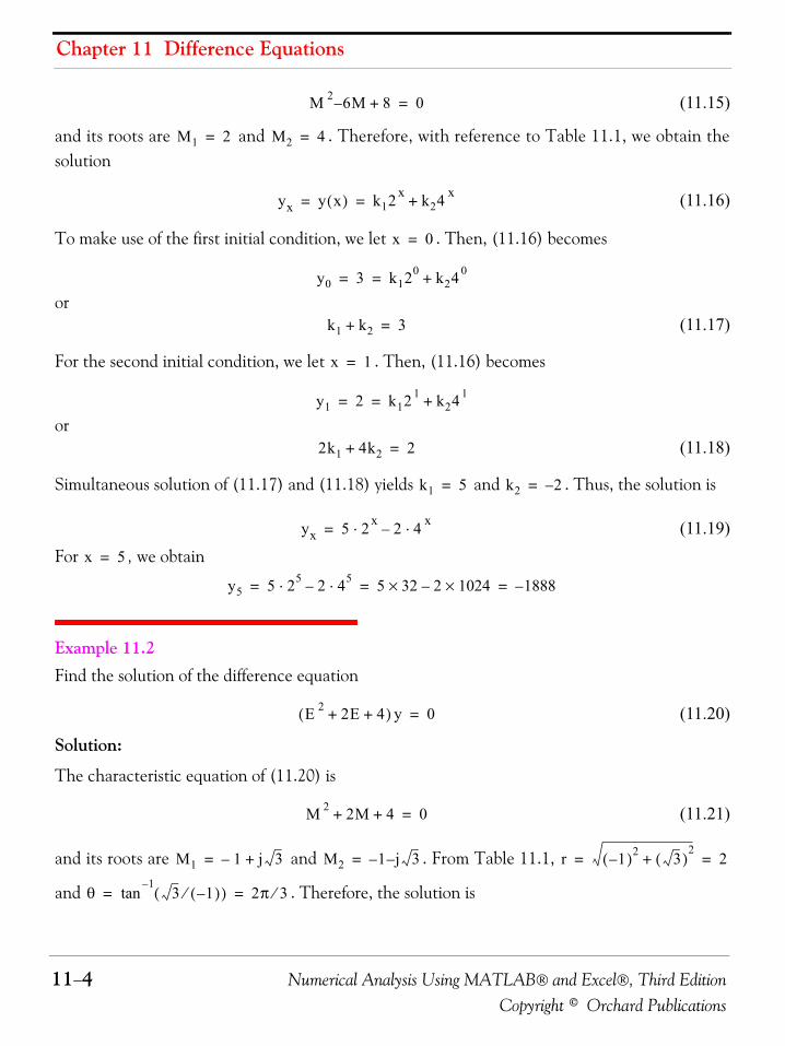
Chapter 11 Difference Equations
11−4 Numerical Analysis Using MATLAB® and Excel®, Third EditionCopyright © Orchard Publications
(11.15)
and its roots are and . Therefore, with reference to Table 11.1, we obtain thesolution
(11.16)
To make use of the first initial condition, we let . Then, (11.16) becomes
or(11.17)
For the second initial condition, we let . Then, (11.16) becomes
or(11.18)
Simultaneous solution of (11.17) and (11.18) yields and . Thus, the solution is
(11.19)For , we obtain
Example 11.2 Find the solution of the difference equation
(11.20)
Solution:
The characteristic equation of (11.20) is
(11.21)
and its roots are and . From Table 11.1,
and . Therefore, the solution is
M 2 6– M 8+ 0=
M1 2= M2 4=
yx y x( ) k12 x k24 x+= =
x 0=
y0 3 k120 k24 0+= =
k1 k2+ 3=
x 1=
y1 2 k12 1 k24 1+= =
2k1 4k2+ 2=
k1 5= k2 2–=
yx 5 2x⋅ 2 4 x⋅–=
x 5=
y5 5 25⋅ 2 45⋅– 5 32× 2 1024×– 1888–= = =
E 2 2E 4+ +( ) y 0=
M 2 2M 4+ + 0=
M1 1– j 3+= M2 1– j– 3= r 1–( )2 3( )2
+ 2= =
θ 3 1–( )⁄( )1–
tan 2π 3⁄= =

Numerical Analysis Using MATLAB® and Excel®, Third Edition 11−5Copyright © Orchard Publications
Definition, Solutions, and Applications
(11.22)
The constants and can be evaluated from the initial conditions.
For non−homogeneous difference equations of the form of (11.10), we combine the particularsolution with the solution of the homogeneous equation shown in (11.11). For the particularsolution, we start with a linear combination of all the terms of the right side, that is, , andwe apply the operator . If any of the terms in the initial choice duplicates a term in the solutionof the homogeneous equation, this choice must be multiplied by until there is no duplicationof terms.
Table 11.2 shows the form of the particular solution for different terms of .
Example 11.3 Find the solution of the difference equation
(11.23)Solution:
The characteristic equation of (11.23) is
(11.24)
TABLE 11.2 Form of the particular solution for a non−homogeneous difference equation
Non−homogeneous difference equation
Form of Particular Solution α (constant) A (constant)
(k = positive integer)
or
or
y 2 x C12π3
------x C22π3
------xsin+cos⎝ ⎠⎛ ⎞=
C1 C2
φ x( )E
x
φ x( )
a2E 2 a1E a0+ +( )y φ x( )=
φ x( ) Y x( )
αxk Akxk Ak 1– xk 1– … A1x A0+ + + +
αkx Akx
α mxcos α msin x A1 mx A2 mxsin+cos
αxklx mxcos αxklx msin x Akxk Ak 1– xk 1– … A1x A0+ + + +( ) lx mxcos
+ Bkxk Bk 1– xk 1– … B1x B0+ + + +( ) lx msin x
E 2 5– E 6+( ) y x 2 x+=
M 2 5– M 6+ 0=
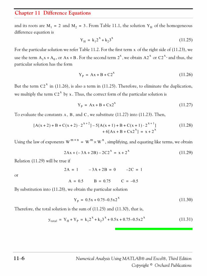
Chapter 11 Difference Equations
11−6 Numerical Analysis Using MATLAB® and Excel®, Third EditionCopyright © Orchard Publications
and its roots are and . From Table 11.1, the solution of the homogeneousdifference equation is
(11.25)
For the particular solution we refer Table 11.2. For the first term of the right side of (11.23), we
use the term , or . For the second term , we obtain or , and thus, theparticular solution has the form
(11.26)
But the term in (11.26), is also a term in (11.25). Therefore, to eliminate the duplication,
we multiply the term by . Thus, the correct form of the particular solution is
(11.27)
To evaluate the constants , , and , we substitute (11.27) into (11.23). Then,
(11.28)
Using the law of exponents , simplifying, and equating like terms, we obtain
(11.29)
Relation (11.29) will be true if
or
By substitution into (11.28), we obtain the particular solution
(11.30)
Therefore, the total solution is the sum of (11.25) and (11.30), that is,
(11.31)
M1 2= M2 3= YH
YH k12 x k23x+=
x
A1x A0+ Ax B+ 2x A2 x C2 x
YP Ax B C2x+ +=
C2 x
C2 x x
YP Ax B Cx2x+ +=
A B C
A x 2+( ) B C x 2+( ) 2 x 2+⋅+ +[ ] 5 A x 1+( ) B C x 1+( ) 2 x 1+⋅+ +[ ]–
6 Ax B Cx2 x+ +[ ]+ x 2 x
+=
W m n+ W m W n×=
2Ax 3A– 2B+( ) 2C2 x–+ x 2 x
+=
2A 1= 3A– 2B+ 0= 2C– 1=
A 0.5= B 0.75= C 0.5–=
YP 0.5x 0.75 0.5– x2 x+=
ytotal YH YP+ k12 x k23 x 0.5x 0.75 0.5– x2 x+ + += =
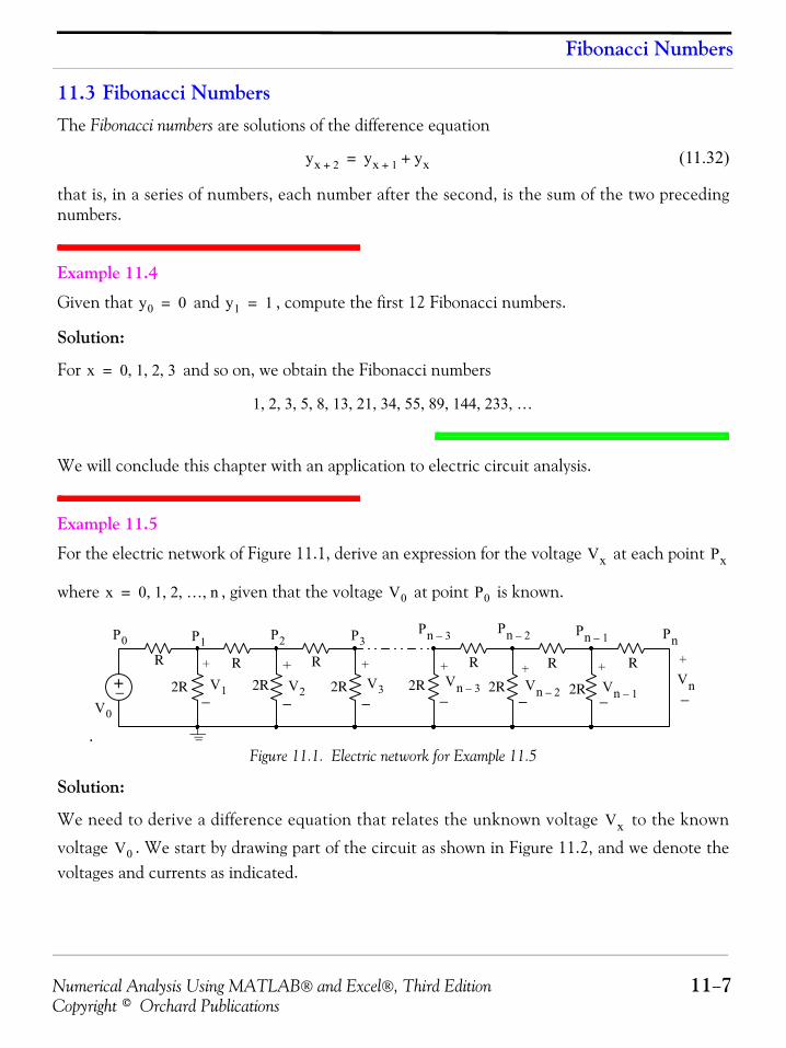
Numerical Analysis Using MATLAB® and Excel®, Third Edition 11−7Copyright © Orchard Publications
Fibonacci Numbers
11.3 Fibonacci NumbersThe Fibonacci numbers are solutions of the difference equation
(11.32)
that is, in a series of numbers, each number after the second, is the sum of the two precedingnumbers.
Example 11.4
Given that and , compute the first 12 Fibonacci numbers.
Solution:
For and so on, we obtain the Fibonacci numbers
We will conclude this chapter with an application to electric circuit analysis.
Example 11.5
For the electric network of Figure 11.1, derive an expression for the voltage at each point
where , given that the voltage at point is known.
.Figure 11.1. Electric network for Example 11.5
Solution:
We need to derive a difference equation that relates the unknown voltage to the known
voltage . We start by drawing part of the circuit as shown in Figure 11.2, and we denote thevoltages and currents as indicated.
yx 2+ yx 1+ yx+=
y0 0= y1 1=
x 0 1 2 3, , ,=
1 2 3 5 8 13 21 34 55 89 144 233 …, , , , , , , , , , , ,
Vx Px
x 0 1 2 … n, , , ,= V0 P0
+−
R RRRRR
2R2R2R2R2R2R
+
−
+
−
+
−
+
−
+
−
+
−
+
−
P0Pn 3–P1 P2 P3 Pn
Pn 2– Pn 1–
V0
Vn 3–V1 V2 V3VnVn 2– Vn 1–
Vx
V0
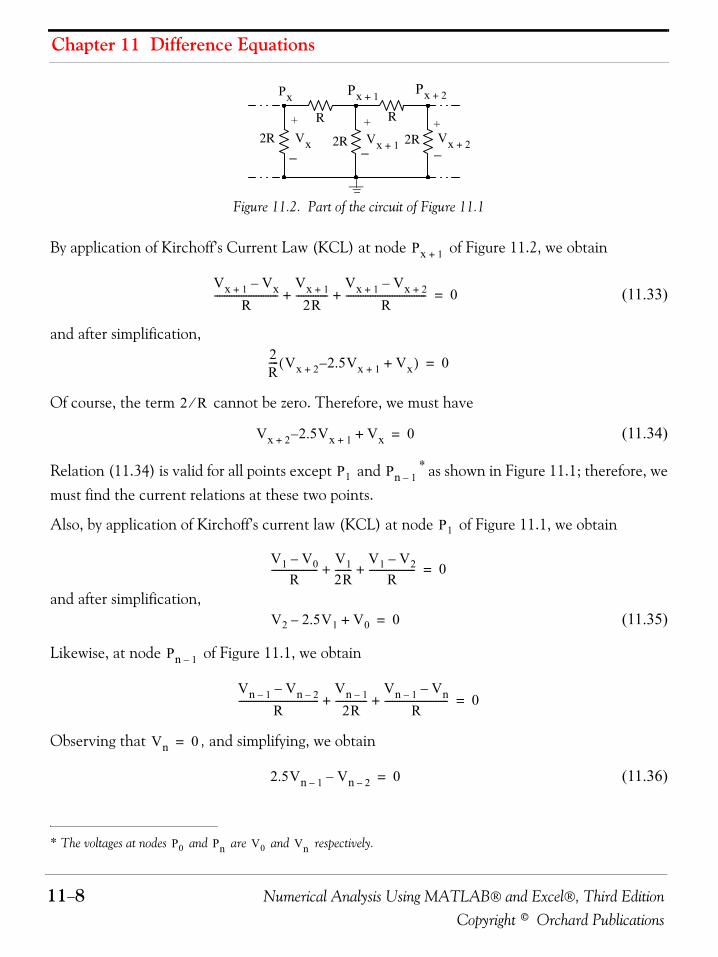
Chapter 11 Difference Equations
11−8 Numerical Analysis Using MATLAB® and Excel®, Third EditionCopyright © Orchard Publications
Figure 11.2. Part of the circuit of Figure 11.1
By application of Kirchoff’s Current Law (KCL) at node of Figure 11.2, we obtain
(11.33)
and after simplification,
Of course, the term cannot be zero. Therefore, we must have
(11.34)
Relation (11.34) is valid for all points except and * as shown in Figure 11.1; therefore, wemust find the current relations at these two points.
Also, by application of Kirchoff’s current law (KCL) at node of Figure 11.1, we obtain
and after simplification, (11.35)
Likewise, at node of Figure 11.1, we obtain
Observing that , and simplifying, we obtain
(11.36)
* The voltages at nodes and are and respectively.
RR
2R2R2R+
−
+
−
+
−Vx 1+
Vx 2+Vx
Px Px 2+Px 1+
Px 1+
Vx 1+ Vx–
R--------------------------
Vx 1+
2R-------------
Vx 1+ Vx 2+–
R---------------------------------+ + 0=
2R---- Vx 2+ 2.5– Vx 1+ Vx+( ) 0=
2 R⁄
Vx 2+ 2.5– Vx 1+ Vx+ 0=
P1 Pn 1–
P0 Pn V0 Vn
P1
V1 V0–
R-------------------
V12R-------
V1 V2–
R-------------------+ + 0=
V2 2.5V1– V0+ 0=
Pn 1–
Vn 1– Vn 2––
R---------------------------------
Vn 1–
2R-------------
Vn 1– Vn–
R--------------------------+ + 0=
Vn 0=
2.5Vn 1– Vn 2–– 0=
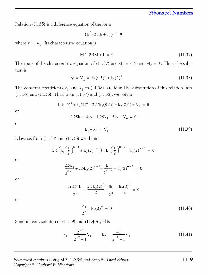
Numerical Analysis Using MATLAB® and Excel®, Third Edition 11−9Copyright © Orchard Publications
Fibonacci Numbers
Relation (11.35) is a difference equation of the form
where . Its characteristic equation is
(11.37)
The roots of the characteristic equation of (11.37) are and . Thus, the solu-tion is
(11.38)
The constant coefficients and in (11.38), are found by substitution of this relation into(11.35) and (11.36). Thus, from (11.37) and (11.38), we obtain
or
or(11.39)
Likewise, from (11.38) and (11.36) we obtain
or
or
or
(11.40)
Simultaneous solution of (11.39) and (11.40) yields
(11.41)
E 2 2.5E– 1+( ) y 0=
y Vx=
M 2 2.5M– 1+ 0=
M1 0.5= M2 2=
y Vx k1 0.5( )x k2 2( )x+= =
k1 k2
k1 0.5( )2 k2 2( )2 2.5 k1 0.5( )1 k2 2( )1+( )– V0+ + 0=
0.25k1 4k2 1.25k1– 5k2– V0+ + 0=
k1 k2+ V0=
2.5 k112---⎝ ⎠
⎛ ⎞ n 1–k2 2( )n 1–
+⎝ ⎠⎛ ⎞ k1
12---⎝ ⎠
⎛ ⎞ n 2–k2 2( )n 2–
–– 0=
2.5k1
2n 1–------------- 2.5k2 2( )n 1– k1
2n 2–-----------– k2 2( )n 2–
–+ 0=
2 2.5( )k1
2 n---------------------
2.5k2 2( )n
2------------------------ 4k1
2 n--------–
k2 2( )n
4----------------–+ 0=
k1
2 n------ k2 2( ) n
+ 0=
k12 2n
2 2n 1–-----------------V0= k2
1–
2 2n 1–-----------------V0=
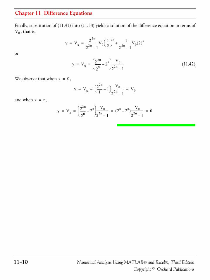
Chapter 11 Difference Equations
11−10 Numerical Analysis Using MATLAB® and Excel®, Third EditionCopyright © Orchard Publications
Finally, substitution of (11.41) into (11.38) yields a solution of the difference equation in terms of, that is,
or
(11.42)
We observe that when ,
and when ,
V0
y Vx2 2n
22n 1–-----------------V0
12---⎝ ⎠
⎛ ⎞ x 1–
2 2n 1–-----------------V0 2( )x+= =
y Vx2 2n
2x-------- 2x
–⎝ ⎠⎜ ⎟⎛ ⎞ V0
22n 1–-----------------= =
x 0=
y Vx22n
1-------- 1–⎝ ⎠⎛ ⎞ V0
2 2n 1–----------------- V0= = =
x n=
y Vx22n
2n-------- 2n–⎝ ⎠⎜ ⎟⎛ ⎞ V0
22n 1–----------------- 2n 2n–( )
V0
22n 1–----------------- 0= = = =
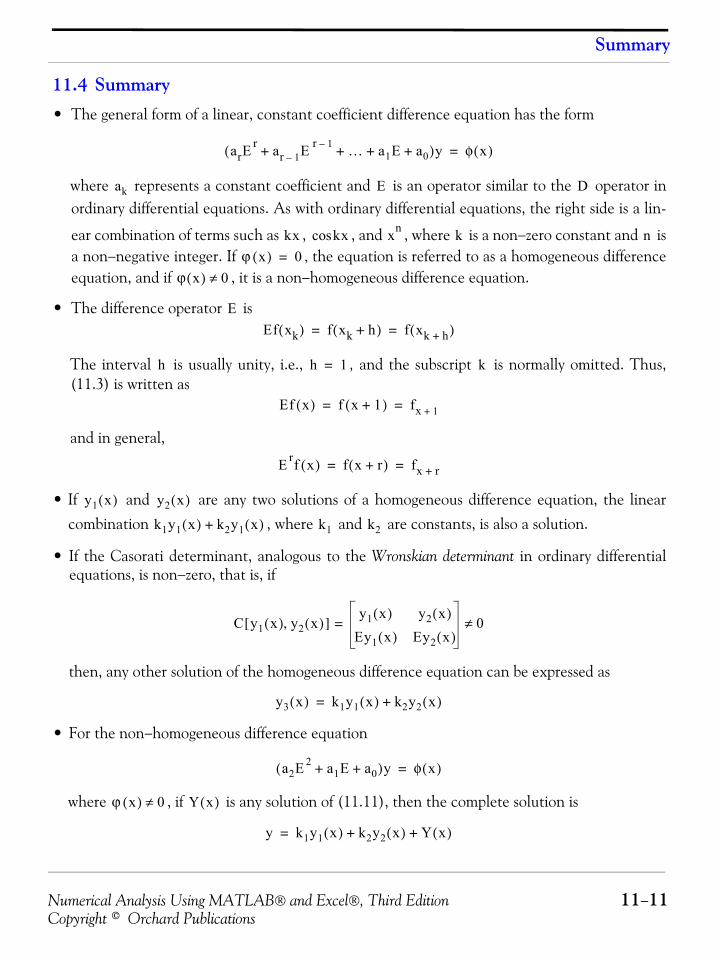
Numerical Analysis Using MATLAB® and Excel®, Third Edition 11−11Copyright © Orchard Publications
Summary
11.4 Summary• The general form of a linear, constant coefficient difference equation has the form
where represents a constant coefficient and is an operator similar to the operator inordinary differential equations. As with ordinary differential equations, the right side is a lin-
ear combination of terms such as , , and , where is a non−zero constant and isa non−negative integer. If , the equation is referred to as a homogeneous differenceequation, and if , it is a non−homogeneous difference equation.
• The difference operator is
The interval is usually unity, i.e., , and the subscript is normally omitted. Thus,(11.3) is written as
and in general,
• If and are any two solutions of a homogeneous difference equation, the linearcombination , where and are constants, is also a solution.
• If the Casorati determinant, analogous to the Wronskian determinant in ordinary differentialequations, is non−zero, that is, if
then, any other solution of the homogeneous difference equation can be expressed as
• For the non−homogeneous difference equation
where , if is any solution of (11.11), then the complete solution is
arEr ar 1– E r 1– …+ + a1E a0+ +( )y φ x( )=
ak E D
kx kxcos xn k nϕ x( ) 0=
ϕ x( ) 0≠
EEf xk( ) f xk h+( ) f xk h+( )= =
h h 1= k
Ef x( ) f x 1+( ) fx 1+= =
E rf x( ) f x r+( ) fx r+= =
y1 x( ) y2 x( )
k1y1 x( ) k2y1 x( )+ k1 k2
C y1 x( ) y2 x( ),[ ]y1 x( ) y2 x( )
Ey1 x( ) Ey2 x( )= 0≠
y3 x( ) k1y1 x( ) k2y2 x( )+=
a2E 2 a1E a0+ +( )y φ x( )=
ϕ x( ) 0≠ Y x( )
y k1y1 x( ) k2y2 x( ) Y x( )+ +=
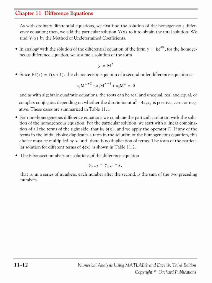
Chapter 11 Difference Equations
11−12 Numerical Analysis Using MATLAB® and Excel®, Third EditionCopyright © Orchard Publications
As with ordinary differential equations, we first find the solution of the homogeneous differ-ence equation; then, we add the particular solution to it to obtain the total solution. Wefind by the Method of Undetermined Coefficients.
• In analogy with the solution of the differential equation of the form , for the homoge-neous difference equation, we assume a solution of the form
• Since , the characteristic equation of a second order difference equation is
and as with algebraic quadratic equations, the roots can be real and unequal, real and equal, or
complex conjugates depending on whether the discriminant is positive, zero, or neg-ative. These cases are summarized in Table 11.1.
• For non−homogeneous difference equations we combine the particular solution with the solu-tion of the homogeneous equation. For the particular solution, we start with a linear combina-tion of all the terms of the right side, that is, , and we apply the operator . If any of theterms in the initial choice duplicates a term in the solution of the homogeneous equation, thischoice must be multiplied by until there is no duplication of terms. The form of the particu-lar solution for different terms of is shown in Table 11.2.
• The Fibonacci numbers are solutions of the difference equation
that is, in a series of numbers, each number after the second, is the sum of the two precedingnumbers.
Y x( )Y x( )
y keax=
y M x=
Ef x( ) f x 1+( )=
a2M x 2+ a1M x 1+ a0M x+ + 0=
a12 4a2a0–
φ x( ) E
xφ x( )
yx 2+ yx 1+ yx+=
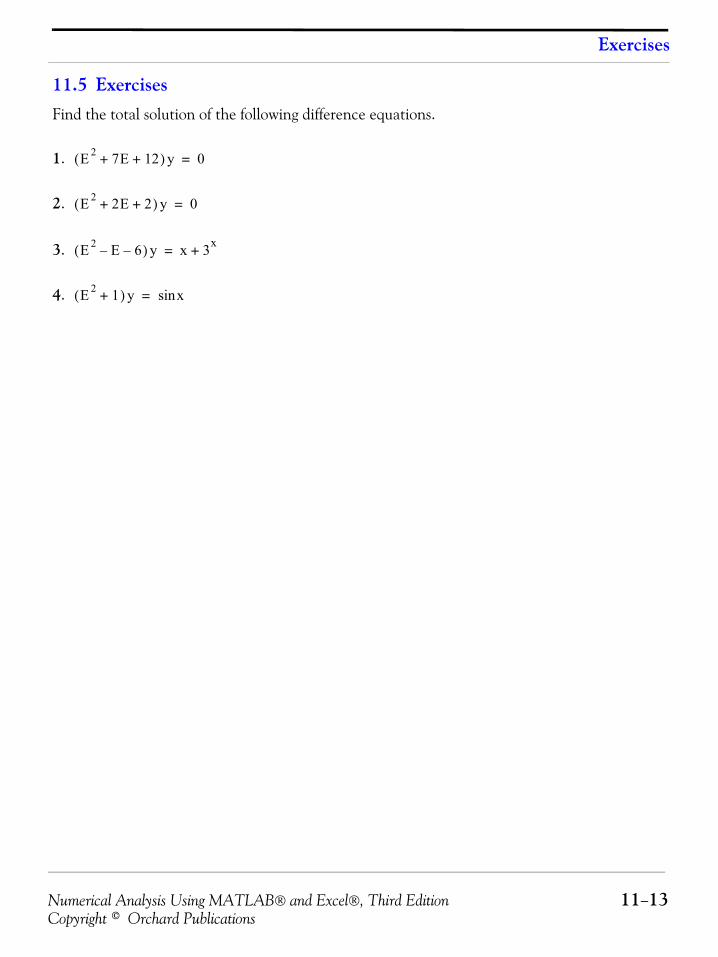
Numerical Analysis Using MATLAB® and Excel®, Third Edition 11−13Copyright © Orchard Publications
Exercises
11.5 ExercisesFind the total solution of the following difference equations.
1.
2.
3.
4.
E 2 7E 12+ +( )y 0=
E 2 2E 2+ +( )y 0=
E 2 E– 6–( )y x 3x+=
E 2 1+( )y xsin=
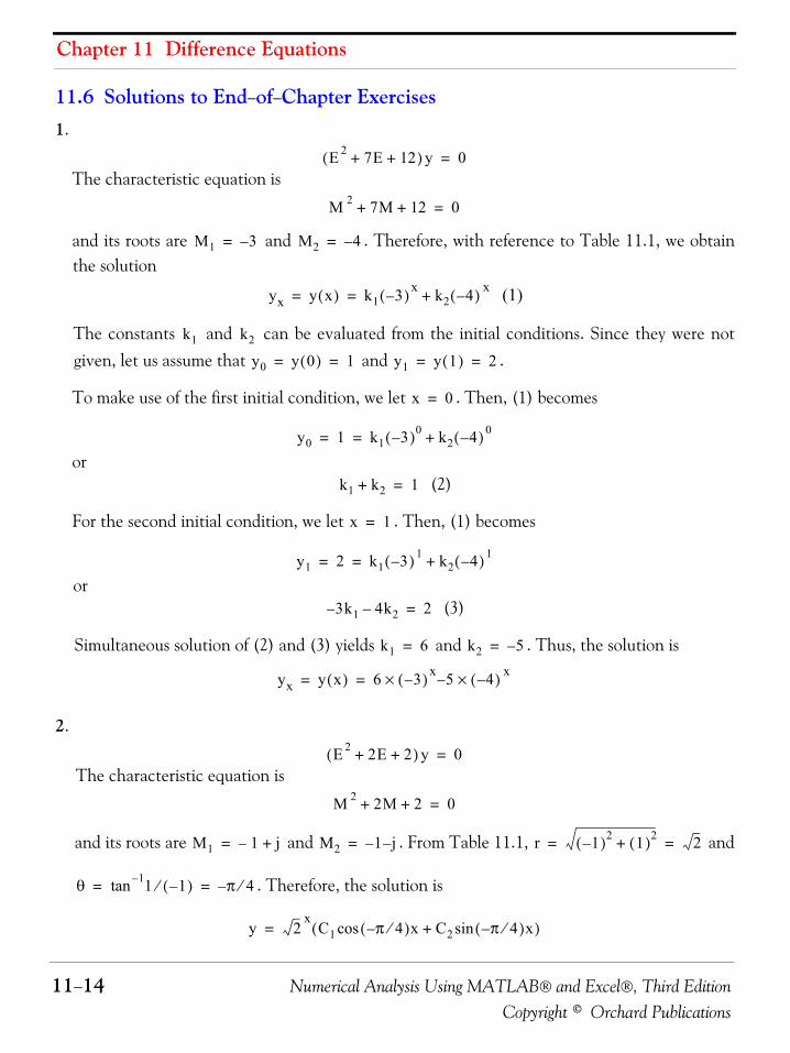
Chapter 11 Difference Equations
11−14 Numerical Analysis Using MATLAB® and Excel®, Third EditionCopyright © Orchard Publications
11.6 Solutions to End−of−Chapter Exercises1.
The characteristic equation is
and its roots are and . Therefore, with reference to Table 11.1, we obtainthe solution
(1)
The constants and can be evaluated from the initial conditions. Since they were notgiven, let us assume that and .
To make use of the first initial condition, we let . Then, (1) becomes
or (2)
For the second initial condition, we let . Then, (1) becomes
or (3)
Simultaneous solution of (2) and (3) yields and . Thus, the solution is
2.
The characteristic equation is
and its roots are and . From Table 11.1, and
. Therefore, the solution is
E 2 7E 12+ +( )y 0=
M 2 7M 12+ + 0=
M1 3–= M2 4–=
yx y x( ) k1 3–( )x k2 4–( ) x+= =
k1 k2
y0 y 0( ) 1= = y1 y 1( ) 2= =
x 0=
y0 1 k1 3–( )0 k2 4–( ) 0+= =
k1 k2+ 1=
x 1=
y1 2 k1 3–( ) 1 k2 4–( ) 1+= =
3– k1 4k2– 2=
k1 6= k2 5–=
yx y x( ) 6 3–( )x× 5– 4–( ) x×= =
E 2 2E 2+ +( )y 0=
M 2 2M 2+ + 0=
M1 1– j+= M2 1– j–= r 1–( )2 1( )2+ 2= =
θ 1 1–( )⁄1–tan π– 4⁄= =
y 2x
C1 π– 4⁄( )x C2 π– 4⁄( )xsin+cos( )=
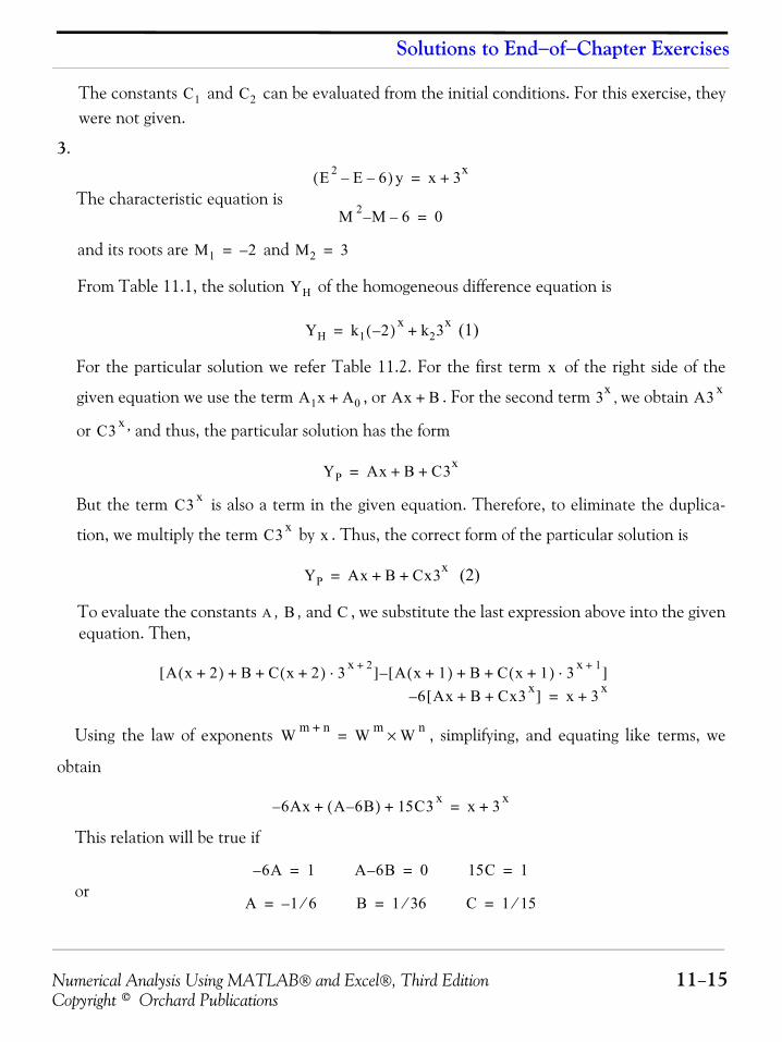
Numerical Analysis Using MATLAB® and Excel®, Third Edition 11−15Copyright © Orchard Publications
Solutions to End−of−Chapter Exercises
The constants and can be evaluated from the initial conditions. For this exercise, theywere not given.
3.
The characteristic equation is
and its roots are and
From Table 11.1, the solution of the homogeneous difference equation is
(1)
For the particular solution we refer Table 11.2. For the first term of the right side of the
given equation we use the term , or . For the second term , we obtain
or , and thus, the particular solution has the form
But the term is also a term in the given equation. Therefore, to eliminate the duplica-
tion, we multiply the term by . Thus, the correct form of the particular solution is
(2)
To evaluate the constants , , and , we substitute the last expression above into the givenequation. Then,
Using the law of exponents , simplifying, and equating like terms, we
obtain
This relation will be true if
or
C1 C2
E 2 E– 6–( )y x 3x+=
M 2 M– 6– 0=
M1 2–= M2 3=
YH
YH k1 2–( ) x k23x+=
x
A1x A0+ Ax B+ 3x A3 x
C3 x
YP Ax B C3x+ +=
C3 x
C3 x x
YP Ax B Cx3x+ +=
A B C
A x 2+( ) B C x 2+( ) 3 x 2+⋅+ +[ ] A x 1+( ) B C x 1+( ) 3 x 1+⋅+ +[ ]–
6– Ax B Cx3 x+ +[ ] x 3 x
+=
W m n+ W m W n×=
6– Ax A 6– B( ) 15C3 x+ + x 3 x
+=
6A– 1= A 6– B 0= 15C 1=
A 1– 6⁄= B 1 36⁄= C 1 15⁄=
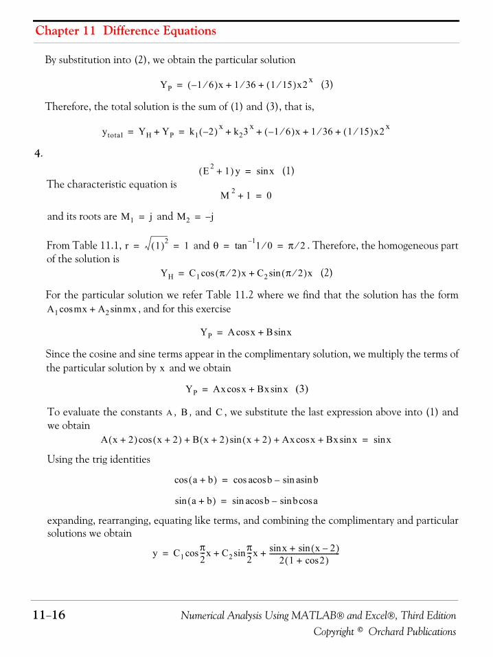
Chapter 11 Difference Equations
11−16 Numerical Analysis Using MATLAB® and Excel®, Third EditionCopyright © Orchard Publications
By substitution into (2), we obtain the particular solution
(3)
Therefore, the total solution is the sum of (1) and (3), that is,
4.
(1)The characteristic equation is
and its roots are and
From Table 11.1, and . Therefore, the homogeneous partof the solution is
(2)
For the particular solution we refer Table 11.2 where we find that the solution has the form, and for this exercise
Since the cosine and sine terms appear in the complimentary solution, we multiply the terms ofthe particular solution by and we obtain
(3)
To evaluate the constants , , and , we substitute the last expression above into (1) andwe obtain
Using the trig identities
expanding, rearranging, equating like terms, and combining the complimentary and particularsolutions we obtain
YP 1– 6⁄( )x 1 36⁄ 1 15⁄( )x2 x+ +=
ytotal YH YP+ k1 2–( ) x k23 x 1– 6⁄( )x 1 36⁄ 1 15⁄( )x2 x+ + + += =
E 2 1+( )y xsin=
M 2 1+ 0=
M1 j= M2 j–=
r 1( )2 1= = θ 1 0⁄1–tan π 2⁄= =
YH C1 π 2⁄( )x C2 π 2⁄( )xsin+cos=
A1 mx A2 mxsin+cos
YP A xcos B xsin+=
x
YP Ax xcos Bx xsin+=
A B C
A x 2+( ) x 2+( ) B x 2+( ) x 2+( ) Ax xcos Bx xsin+ +sin+cos xsin=
a b+( )cos b basinsin–acoscos=
a b+( )sin b b acossin–acossin=
y C1π2---x C2
π2---x x x 2–( )sin+sin
2 1 2cos+( )------------------------------------------+sin+cos=
Numerical Analysis Using MATLAB® and Excel®, Third Edition 12−1Copyright © Orchard Publications
Chapter 12
Partial Fraction Expansion
his chapter is an introduction to partial fraction expansion methods. In elementary algebrawe learned how to combine fractions over a common denominator. Partial fraction expan-sion is the reverse process and splits a rational expression into a sum of fractions having
simpler denominators.
12.1 Partial Fraction ExpansionThe partial fraction expansion method is used extensively in integration and in finding theinverses of the Laplace, Fourier, and Z transforms. This method allows us to decompose a ratio-nal polynomial into smaller rational polynomials with simpler denominators, from which we caneasily recognize their integrals or inverse transformations. In the subsequent discussion we willdiscuss the partial fraction expansion method and we will illustrate with several examples. Wewill also use the MATLAB residue(r,p,k) function which returns the residues (coefficients) r of apartial fraction expansion, the poles p and the direct terms k. There are no direct terms if thehighest power of the numerator is less than that of the denominator.
Let
(12.1)
where and are polynomials and thus (12.1) can be expressed as
(12.2)
The coefficients and for are real numbers and, for the present discus-sion, we have assumed that the highest power of is less than the highest power of , i.e.,
. In this case, is a proper rational function. If , is an improper rational function.
It is very convenient to make the coefficient of in (12.2) unity; to do this, we rewrite it as
(12.3)
T
F s( ) N s( )D s( )-----------=
N s( ) D s( )
F s( ) N s( )D s( )-----------
bmsm bm 1– sm 1– bm 2– sm 2– … b1s b0+ + + + +
ansn an 1– sn 1– an 2– sn 2– … a1s a0+ + + + +--------------------------------------------------------------------------------------------------------------------= =
ak bk k 0 1 2 … n, , , ,=
N s( ) D s( )m n< F s( ) m n≥ F s( )
an sn
F s( ) N s( )D s( )-----------
1an----- bmsm bm 1– sm 1– bm 2– sm 2– … b1s b0+ + + + +( )
sn an 1–
an-----------sn 1– an 2–
an-----------sn 2– …
a1an-----s
a0an-----+ + + + +
-------------------------------------------------------------------------------------------------------------------------------= =
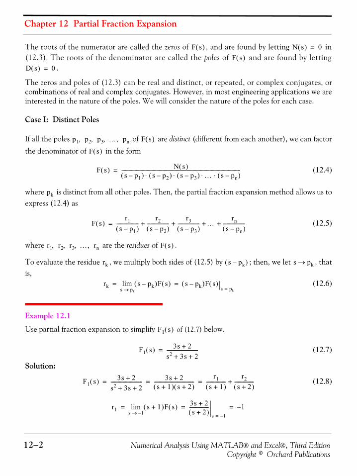
Chapter 12 Partial Fraction Expansion
12−2 Numerical Analysis Using MATLAB® and Excel®, Third EditionCopyright © Orchard Publications
The roots of the numerator are called the zeros of , and are found by letting in(12.3). The roots of the denominator are called the poles of and are found by letting
.
The zeros and poles of (12.3) can be real and distinct, or repeated, or complex conjugates, orcombinations of real and complex conjugates. However, in most engineering applications we areinterested in the nature of the poles. We will consider the nature of the poles for each case.
Case I: Distinct Poles
If all the poles of are distinct (different from each another), we can factorthe denominator of in the form
(12.4)
where is distinct from all other poles. Then, the partial fraction expansion method allows us toexpress (12.4) as
(12.5)
where are the residues of .
To evaluate the residue , we multiply both sides of (12.5) by ; then, we let , thatis,
(12.6)
Example 12.1
Use partial fraction expansion to simplify of (12.7) below.
(12.7)
Solution:
(12.8)
F s( ) N s( ) 0=
F s( )D s( ) 0=
p1 p2 p3 … pn, , , , F s( )
F s( )
F s( ) N s( )s p1–( ) s p2–( ) s p3–( ) … s pn–( )⋅ ⋅ ⋅ ⋅
--------------------------------------------------------------------------------------------------=
pk
F s( )r1
s p1–( )------------------
r2s p2–( )
------------------r3
s p3–( )------------------ …
rns pn–( )
------------------+ + + +=
r1 r2 r3 … rn, , , , F s( )
rk s pk–( ) s pk→
rk s pk–( )F s( )s pk→lim s pk–( )F s( )
s pk== =
F1 s( )
F1 s( ) 3s 2+s2 3s 2+ +--------------------------=
F1 s( ) 3s 2+s2 3s 2+ +-------------------------- 3s 2+
s 1+( ) s 2+( )---------------------------------
r1s 1+( )
----------------r2
s 2+( )----------------+= = =
r1 s 1+( )F s( )s 1–→lim 3s 2+
s 2+( )----------------
s 1–=
1–= = =
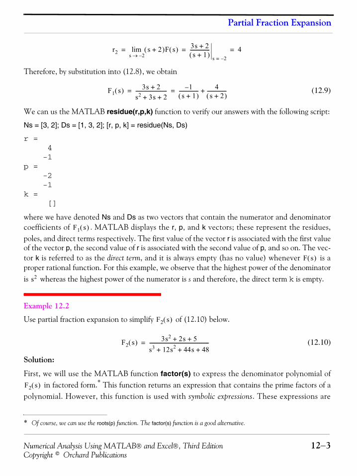
Numerical Analysis Using MATLAB® and Excel®, Third Edition 12−3Copyright © Orchard Publications
Partial Fraction Expansion
Therefore, by substitution into (12.8), we obtain
(12.9)
We can us the MATLAB residue(r,p,k) function to verify our answers with the following script:
Ns = [3, 2]; Ds = [1, 3, 2]; [r, p, k] = residue(Ns, Ds)
r = 4 -1p = -2 -1k = []
where we have denoted Ns and Ds as two vectors that contain the numerator and denominatorcoefficients of . MATLAB displays the r, p, and k vectors; these represent the residues,poles, and direct terms respectively. The first value of the vector r is associated with the first valueof the vector p, the second value of r is associated with the second value of p, and so on. The vec-tor k is referred to as the direct term, and it is always empty (has no value) whenever is aproper rational function. For this example, we observe that the highest power of the denominatoris whereas the highest power of the numerator is s and therefore, the direct term k is empty.
Example 12.2
Use partial fraction expansion to simplify of (12.10) below.
(12.10)
Solution:
First, we will use the MATLAB function factor(s) to express the denominator polynomial of in factored form.* This function returns an expression that contains the prime factors of a
polynomial. However, this function is used with symbolic expressions. These expressions are
* Of course, we can use the roots(p) function. The factor(s) function is a good alternative.
r2 s 2+( )F s( )s 2–→lim 3s 2+
s 1+( )----------------
s 2–=
4= = =
F1 s( ) 3s 2+s2 3s 2+ +-------------------------- 1–
s 1+( )---------------- 4
s 2+( )----------------+= =
F1 s( )
F s( )
s2
F2 s( )
F2 s( ) 3s2 2s 5+ +
s3 12s+ 2 44s 48+ +-------------------------------------------------=
F2 s( )
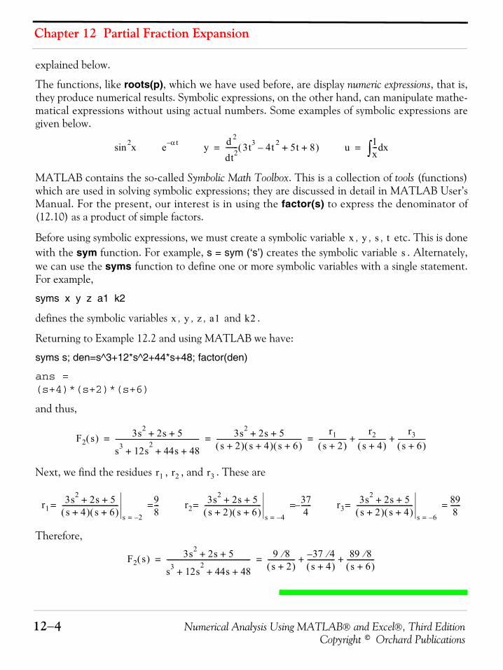
Chapter 12 Partial Fraction Expansion
12−4 Numerical Analysis Using MATLAB® and Excel®, Third EditionCopyright © Orchard Publications
explained below.
The functions, like roots(p), which we have used before, are display numeric expressions, that is,they produce numerical results. Symbolic expressions, on the other hand, can manipulate mathe-matical expressions without using actual numbers. Some examples of symbolic expressions aregiven below.
MATLAB contains the so-called Symbolic Math Toolbox. This is a collection of tools (functions)which are used in solving symbolic expressions; they are discussed in detail in MATLAB User’sManual. For the present, our interest is in using the factor(s) to express the denominator of(12.10) as a product of simple factors.
Before using symbolic expressions, we must create a symbolic variable , , , etc. This is donewith the sym function. For example, s = sym (‘s’) creates the symbolic variable . Alternately,we can use the syms function to define one or more symbolic variables with a single statement.For example,
syms x y z a1 k2
defines the symbolic variables , , , and .
Returning to Example 12.2 and using MATLAB we have:
syms s; den=s^3+12*s^2+44*s+48; factor(den)
ans =(s+4)*(s+2)*(s+6)
and thus,
Next, we find the residues , , and . These are
Therefore,
x2sin e αt– y d 2
dt2------- 3t3 4t 2– 5t 8+ +( )= u 1
x--- xd∫=
x y s ts
x y z a1 k2
F2 s( ) 3s2 2s 5+ +
s3 12s+2
44s 48+ +------------------------------------------------- 3s2 2s 5+ +
s 2+( ) s 4+( ) s 6+( )--------------------------------------------------
r1s 2+( )
----------------r2
s 4+( )----------------
r3s 6+( )
----------------+ += = =
r1 r2 r3
r13s2 2s 5+ +s 4+( ) s 6+( )
---------------------------------s 2–=
98---= = r2
3s2 2s 5+ +s 2+( ) s 6+( )
---------------------------------s 4–=
= 374------–= r3
3s2 2s 5+ +s 2+( ) s 4+( )
---------------------------------s 6–=
= 898
------=
F2 s( ) 3s2 2s 5+ +
s3 12s+2
44s 48+ +------------------------------------------------- 9 8⁄
s 2+( )---------------- 37 4⁄–
s 4+( )---------------- 89 8⁄
s 6+( )----------------+ += =
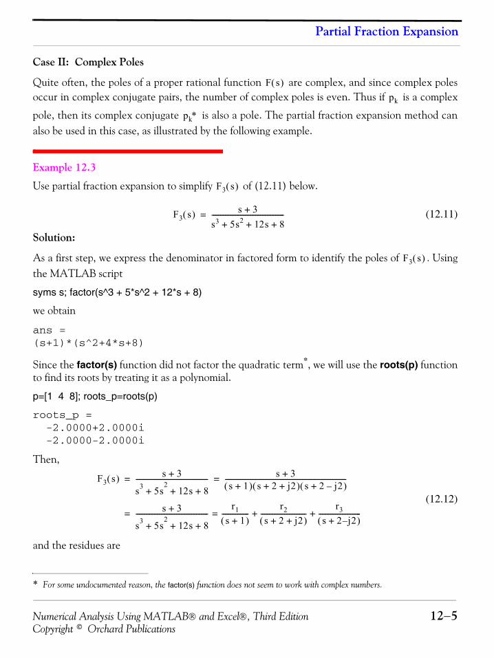
Numerical Analysis Using MATLAB® and Excel®, Third Edition 12−5Copyright © Orchard Publications
Partial Fraction Expansion
Case II: Complex Poles
Quite often, the poles of a proper rational function are complex, and since complex polesoccur in complex conjugate pairs, the number of complex poles is even. Thus if is a complex
pole, then its complex conjugate is also a pole. The partial fraction expansion method canalso be used in this case, as illustrated by the following example.
Example 12.3
Use partial fraction expansion to simplify of (12.11) below.
(12.11)
Solution:
As a first step, we express the denominator in factored form to identify the poles of . Usingthe MATLAB script
syms s; factor(s^3 + 5*s^2 + 12*s + 8)
we obtain
ans =(s+1)*(s^2+4*s+8)
Since the factor(s) function did not factor the quadratic term*, we will use the roots(p) functionto find its roots by treating it as a polynomial.
p=[1 4 8]; roots_p=roots(p)
roots_p = -2.0000+2.0000i -2.0000-2.0000i
Then,
(12.12)
and the residues are
* For some undocumented reason, the factor(s) function does not seem to work with complex numbers.
F s( )pk
pk∗
F3 s( )
F3 s( ) s 3+
s3 5s+ 2 12s 8+ +-------------------------------------------=
F3 s( )
F3 s( ) s 3+
s3 5s+2
12s 8+ +------------------------------------------- s 3+
s 1+( ) s 2 j2+ +( ) s 2 j2–+( )------------------------------------------------------------------------= =
s 3+
s3 5s+2
12s 8+ +-------------------------------------------
r1s 1+( )
----------------r2
s 2 j2+ +( )---------------------------
r3s 2 j– 2+( )
-------------------------+ +==
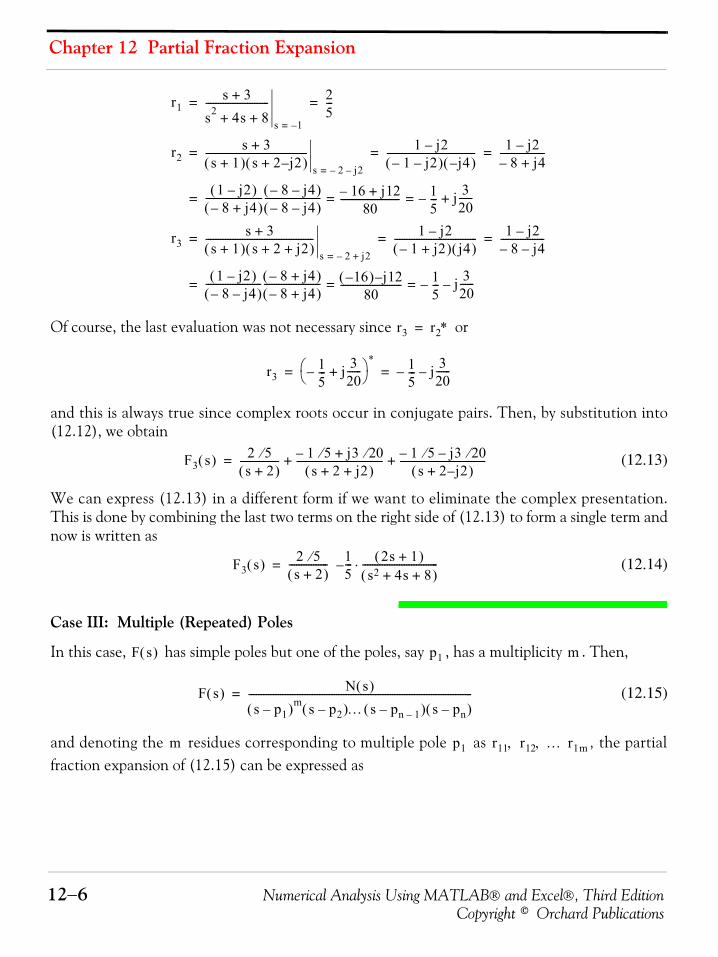
Chapter 12 Partial Fraction Expansion
12−6 Numerical Analysis Using MATLAB® and Excel®, Third EditionCopyright © Orchard Publications
Of course, the last evaluation was not necessary since or
and this is always true since complex roots occur in conjugate pairs. Then, by substitution into(12.12), we obtain
(12.13)
We can express (12.13) in a different form if we want to eliminate the complex presentation.This is done by combining the last two terms on the right side of (12.13) to form a single term andnow is written as
(12.14)
Case III: Multiple (Repeated) Poles
In this case, has simple poles but one of the poles, say , has a multiplicity . Then,
(12.15)
and denoting the residues corresponding to multiple pole as , the partialfraction expansion of (12.15) can be expressed as
r1s 3+
s2 4s 8+ +--------------------------
s 1–=
25---= =
r2s 3+
s 1+( ) s 2 j– 2+( )------------------------------------------
s 2– j2–=
1 j2–1– j2–( ) j4–( )
------------------------------------ 1 j2–8– j4+
------------------= = =
1 j2–( )8– j4+( )
----------------------- 8– j4–( )8– j4–( )
----------------------- 16– j12+80
------------------------ 15---– j 3
20------+= ==
r3s 3+
s 1+( ) s 2 j2+ +( )--------------------------------------------
s 2– j2+=
1 j2–1– j2+( ) j4( )
---------------------------------- 1 j2–8– j4–
------------------= = =
1 j2–( )8– j4–( )
----------------------- 8– j4+( )8– j4+( )
----------------------- 16–( ) j– 1280
------------------------- 15---– j 3
20------–= ==
r3 r2∗=
r315---– j 3
20------+⎝ ⎠
⎛ ⎞ * 15---– j 3
20------–= =
F3 s( ) 2 5⁄s 2+( )
---------------- 1 5⁄– j3 20⁄+s 2 j2+ +( )
----------------------------------- 1 5⁄– j3 20⁄–s 2 j– 2+( )
-----------------------------------+ +=
F3 s( ) 2 5⁄s 2+( )
---------------- 15--- 2s 1+( )
s2 4s 8+ +( )-------------------------------⋅–=
F s( ) p1 m
F s( ) N s( )
s p1–( )m s p2–( )… s pn 1––( ) s pn–( )--------------------------------------------------------------------------------------------=
m p1 r11 r12 … r1m, ,
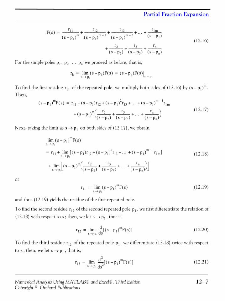
Numerical Analysis Using MATLAB® and Excel®, Third Edition 12−7Copyright © Orchard Publications
Partial Fraction Expansion
(12.16)
For the simple poles we proceed as before, that is,
To find the first residue of the repeated pole, we multiply both sides of (12.16) by .Then,
(12.17)
Next, taking the limit as on both sides of (12.17), we obtain
(12.18)
or
(12.19)
and thus (12.19) yields the residue of the first repeated pole.
To find the second residue of the second repeated pole , we first differentiate the relation of(12.18) with respect to ; then, we let , that is,
(12.20)
To find the third residue of the repeated pole , we differentiate (12.18) twice with respectto ; then, we let , that is,
(12.21)
F s( )r11
s p1–( )m----------------------
r12
s p1–( )m 1–----------------------------
r13
s p1–( )m 2–---------------------------- …
r1ms p1–( )
------------------+ + + +=
r2
s p2–( )------------------
r3s p3–( )
------------------rn
s pn–( )------------------+ + +
p1 p2 … pn, ,
rk s pk–( )F s( )s pk→lim s pk–( )F s( )
s pk== =
r11 s p1–( )m
s p1–( )mF s( ) r11 s p1–( )r12 s p1–( )2r13 … s p1–( )m 1– r1m+ + + +=
s p1–( )m r2s p2–( )
------------------r3
s p3–( )------------------ …
rns pn–( )
------------------+ + +⎝ ⎠⎛ ⎞+
s p1→
s p1–( )mF s( )s p1→lim
r11 s p1–( )r12 s p1–( )2r13 … s p1–( )m 1– r1m+ + +[ ]s p1→lim+=
s p1–( )m r2s p2–( )
------------------r3
s p3–( )------------------ …
rns pn–( )
------------------+ + +⎝ ⎠⎛ ⎞
s p1→lim+
r11 s p1–( )mF s( )s p1→lim=
r12 p1
s s p1→
r12dds-----
s p1→lim s p1–( )mF s( )[ ]=
r13 p1
s s p1→
r13d 2
ds2--------
s p1→lim s p1–( )mF s( )[ ]=
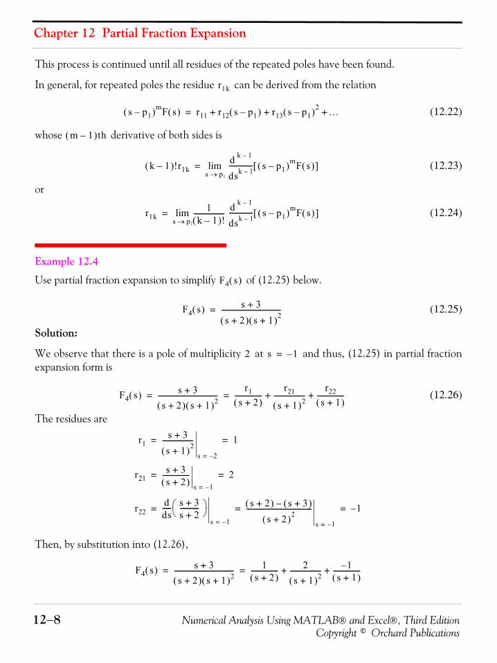
Chapter 12 Partial Fraction Expansion
12−8 Numerical Analysis Using MATLAB® and Excel®, Third EditionCopyright © Orchard Publications
This process is continued until all residues of the repeated poles have been found.
In general, for repeated poles the residue can be derived from the relation
(12.22)
whose derivative of both sides is
(12.23)
or
(12.24)
Example 12.4
Use partial fraction expansion to simplify of (12.25) below.
(12.25)
Solution:
We observe that there is a pole of multiplicity at and thus, (12.25) in partial fractionexpansion form is
(12.26)
The residues are
Then, by substitution into (12.26),
r1k
s p1–( )mF s( ) r11 r12 s p1–( ) r13 s p1–( )2 …+ + +=
m 1–( )th
k 1–( )!r1kd k 1–
dsk 1–-------------- s p1–( )mF s( )[ ]
s p1→lim=
r1k1
k 1–( )!------------------
s p1→lim d k 1–
dsk 1–-------------- s p1–( )mF s( )[ ]=
F4 s( )
F4 s( ) s 3+
s 2+( ) s 1+( )2-----------------------------------=
2 s 1–=
F4 s( ) s 3+
s 2+( ) s 1+( )2-----------------------------------
r1s 2+( )
----------------r21
s 1+( )2------------------
r22s 1+( )
----------------+ += =
r1s 3+
s 1+( )2------------------
s 2–=
1= =
r21s 3+s 2+( )
----------------s 1–=
2= =
r22dds----- s 3+
s 2+-----------⎝ ⎠
⎛ ⎞
s 1–=
s 2+( ) s 3+( )–
s 2+( )2---------------------------------------
s 1–=
1–= = =
F4 s( ) s 3+
s 2+( ) s 1+( )2----------------------------------- 1
s 2+( )---------------- 2
s 1+( )2------------------ 1–
s 1+( )----------------+ += =
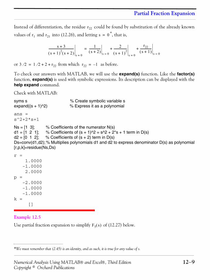
Numerical Analysis Using MATLAB® and Excel®, Third Edition 12−9Copyright © Orchard Publications
Partial Fraction Expansion
Instead of differentiation, the residue could be found by substitution of the already known
values of and into (12.26), and letting *, that is,
or from which as before.
To check our answers with MATLAB, we will use the expand(s) function. Like the factor(s)function, expand(s) is used with symbolic expressions. Its description can be displayed with thehelp expand command.
Check with MATLAB:
syms s % Create symbolic variable sexpand((s + 1)^2) % Express it as a polynomial
ans =s^2+2*s+1
Ns = [1 3]; % Coefficients of the numerator N(s) d1 = [1 2 1]; % Coefficients of (s + 1)^2 = s^2 + 2*s + 1 term in D(s)d2 = [0 1 2]; % Coefficients of (s + 2) term in D(s)Ds=conv(d1,d2); % Multiplies polynomials d1 and d2 to express denominator D(s) as polynomial[r,p,k]=residue(Ns,Ds)
r = 1.0000 -1.0000 2.0000p = -2.0000 -1.0000 -1.0000k = []
Example 12.5
Use partial fraction expansion to simplify of (12.27) below.
*We must remember that (2.45) is an identity, and as such, it is true for any value of s.
r22
r1 r21 s 0=
s 3+
s 1+( )2 s 2+( )-----------------------------------
s 0=
1s 2+( )
----------------s 0=
2s 1+( )2
------------------s 0=
r22s 1+( )
----------------s 0=
+ +=
3 2⁄ 1 2⁄ 2 r22+ += r22 1–=
F5 s( )
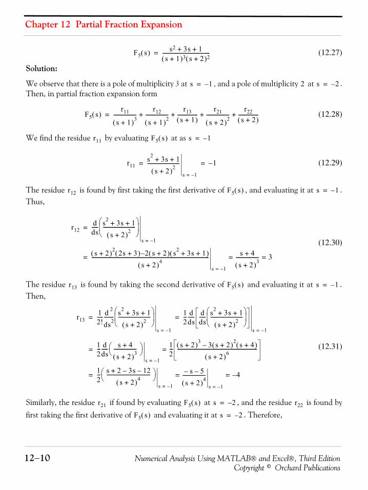
Chapter 12 Partial Fraction Expansion
12−10 Numerical Analysis Using MATLAB® and Excel®, Third EditionCopyright © Orchard Publications
(12.27)
Solution:
We observe that there is a pole of multiplicity 3 at , and a pole of multiplicity at .Then, in partial fraction expansion form
(12.28)
We find the residue by evaluating at as
(12.29)
The residue is found by first taking the first derivative of , and evaluating it at .Thus,
(12.30)
The residue is found by taking the second derivative of and evaluating it at .Then,
(12.31)
Similarly, the residue if found by evaluating at , and the residue is found byfirst taking the first derivative of and evaluating it at . Therefore,
F5 s( ) s2 3+ s 1+s 1+( )3 s 2+( )2
--------------------------------------=
s 1–= 2 s 2–=
F5 s( )r11
s 1+( )3------------------
r12
s 1+( )2------------------
r13s 1+( )
----------------r21
s 2+( )2------------------
r22s 2+( )
----------------+ + + +=
r11 F5 s( ) s 1–=
r11s2 3+ s 1+
s 2+( )2--------------------------
s 1–=
1–= =
r12 F5 s( ) s 1–=
r12dds----- s2 3+ s 1+
s 2+( )2--------------------------⎝ ⎠⎜ ⎟⎛ ⎞
s 1–=
=
s 2+( )2 2s 3+( ) 2 s 2+( ) s2 3+ s 1+( )–
s 2+( )4----------------------------------------------------------------------------------------------
s 1–=
s 4+
s 2+( )3------------------= 3==
r13 F5 s( ) s 1–=
r1312!----- d 2
ds2-------- s2 3+ s 1+
s 2+( )2--------------------------⎝ ⎠⎜ ⎟⎛ ⎞
s 1–=
12--- d
ds----- d
ds----- s2 3+ s 1+
s 2+( )2--------------------------⎝ ⎠⎜ ⎟⎛ ⎞
s 1–=
= =
12--- d
ds----- s 4+
s 2+( )3------------------⎝ ⎠
⎛ ⎞
s 1–=
12--- s 2+( )3 3 s 2+( )2 s 4+( )–
s 2+( )6----------------------------------------------------------------==
12--- s 2 3s– 12–+
s 2+( )4-----------------------------------⎝ ⎠
⎛ ⎞
s 1–=
s– 5–
s 2+( )4------------------
s 1–=
4–= ==
r21 F5 s( ) s 2–= r22
F5 s( ) s 2–=
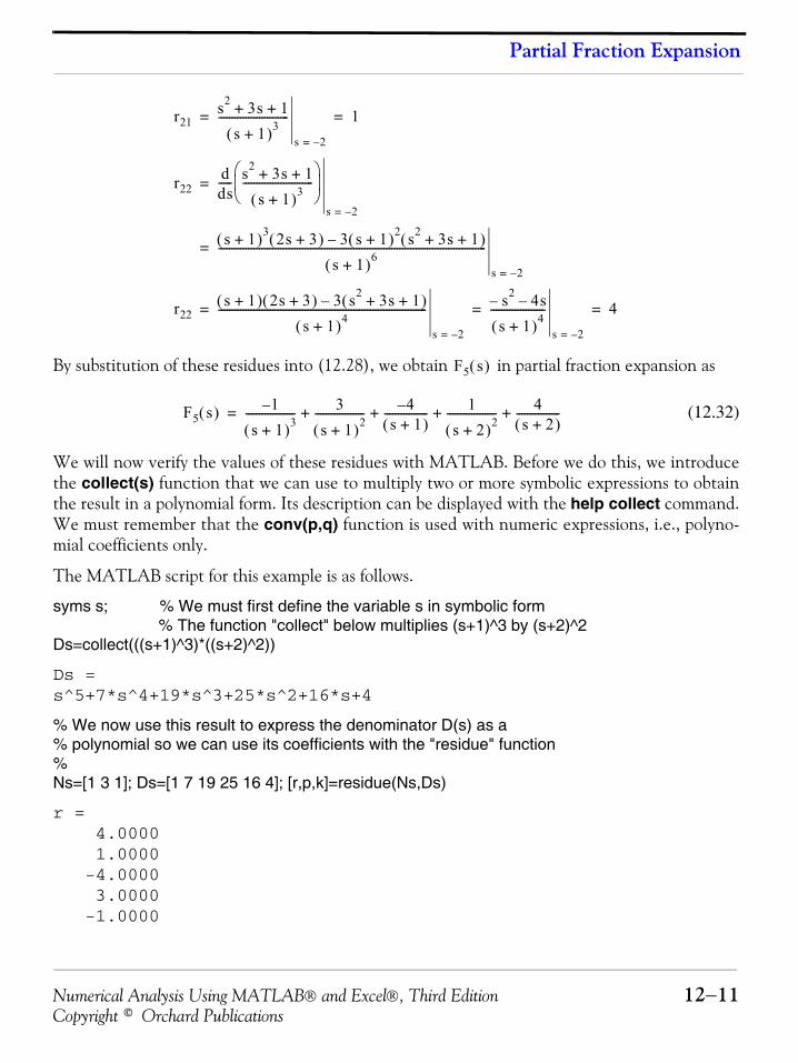
Numerical Analysis Using MATLAB® and Excel®, Third Edition 12−11Copyright © Orchard Publications
Partial Fraction Expansion
By substitution of these residues into (12.28), we obtain in partial fraction expansion as
(12.32)
We will now verify the values of these residues with MATLAB. Before we do this, we introducethe collect(s) function that we can use to multiply two or more symbolic expressions to obtainthe result in a polynomial form. Its description can be displayed with the help collect command.We must remember that the conv(p,q) function is used with numeric expressions, i.e., polyno-mial coefficients only.
The MATLAB script for this example is as follows.
syms s; % We must first define the variable s in symbolic form% The function "collect" below multiplies (s+1)^3 by (s+2)^2
Ds=collect(((s+1)^3)*((s+2)^2))
Ds =s^5+7*s^4+19*s^3+25*s^2+16*s+4
% We now use this result to express the denominator D(s) as a% polynomial so we can use its coefficients with the "residue" function% Ns=[1 3 1]; Ds=[1 7 19 25 16 4]; [r,p,k]=residue(Ns,Ds)
r = 4.0000 1.0000 -4.0000 3.0000 -1.0000
r21s2 3+ s 1+
s 1+( )3--------------------------
s 2–=
1= =
r22dds----- s2 3+ s 1+
s 1+( )3--------------------------⎝ ⎠⎜ ⎟⎛ ⎞
s 2–=
=
s 1+( )3 2s 3+( ) 3 s 1+( )2 s2 3+ s 1+( )–
s 1+( )6---------------------------------------------------------------------------------------------------
s 2–=
=
r22s 1+( ) 2s 3+( ) 3 s2 3+ s 1+( )–
s 1+( )4-----------------------------------------------------------------------------
s 2–=
s2– 4s–
s 1+( )4--------------------
s 2–=
4= = =
F5 s( )
F5 s( ) 1–
s 1+( )3------------------ 3
s 1+( )2------------------ 4–
s 1+( )---------------- 1
s 2+( )2------------------ 4
s 2+( )----------------+ + + +=
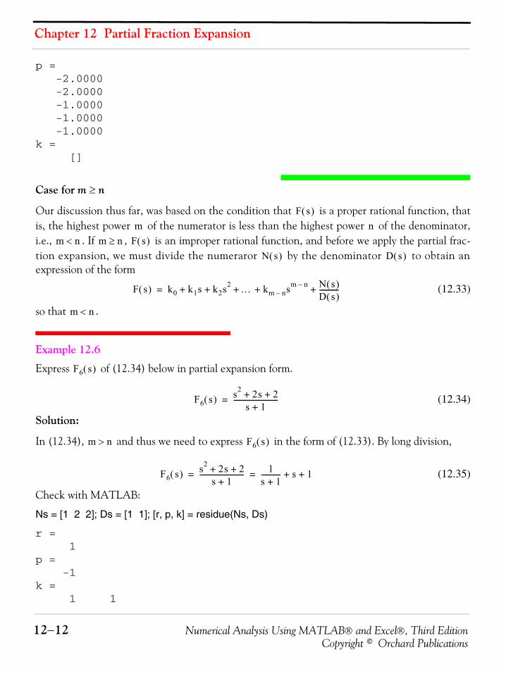
Chapter 12 Partial Fraction Expansion
12−12 Numerical Analysis Using MATLAB® and Excel®, Third EditionCopyright © Orchard Publications
p = -2.0000 -2.0000 -1.0000 -1.0000 -1.0000k = []
Case for m ≥ n
Our discussion thus far, was based on the condition that is a proper rational function, thatis, the highest power of the numerator is less than the highest power of the denominator,i.e., . If , is an improper rational function, and before we apply the partial frac-tion expansion, we must divide the numeraror by the denominator to obtain anexpression of the form
(12.33)
so that .
Example 12.6
Express of (12.34) below in partial expansion form.
(12.34)
Solution:
In (12.34), and thus we need to express in the form of (12.33). By long division,
(12.35)
Check with MATLAB:
Ns = [1 2 2]; Ds = [1 1]; [r, p, k] = residue(Ns, Ds)
r = 1p = -1k = 1 1
F s( )m n
m n< m n≥ F s( )N s( ) D s( )
F s( ) k0 k1s k2s2 … km n– sm n– N s( )D s( )-----------+ + + + +=
m n<
F6 s( )
F6 s( ) s2 2s 2+ +s 1+
--------------------------=
m n> F6 s( )
F6 s( ) s2 2s 2+ +s 1+
-------------------------- 1s 1+----------- s 1+ += =
Numerical Analysis Using MATLAB® and Excel®, Third Edition 12−13Copyright © Orchard Publications
Alternate Method of Partial Fraction Expansion
The direct terms are the coefficients of the term and the constant in (2.54).
12.2 Alternate Method of Partial Fraction Expansion
The partial fraction expansion method can also be performed by the equating the numerators proce-dure thereby making the denominators of both sides the same, and then equating the numerators.We assume that the degree on the numerator is less than the degree of the denominator. Ifnot, we first perform a long division and then work with the quotient and the remainder asbefore.
We also assume that the denominator can be expressed as a product of real linear and qua-dratic factors. If these assumptions prevail, we let be a linear factor of and we suppose
that is the highest power of that divides . Then, we can express as
(12.36)
Next, let be a quadratic factor of and suppose that is the highestpower of this factor that divides . Now, we perform the following steps:
1. To this factor, we assign the sum of n partial fractions as shown below.
(12.37)
2. We repeat Step 1 for each of the distinct linear and quadratic factors of .
3. We set the given equal to the sum of these partial fractions.
4. We multiply each term of the right side by the appropriate factor to make the denominators ofboth sides equal.
5. We arrange the terms of both sides in decreasing powers of .
6. We equate the coefficients of corresponding powers of s.
7. We solve the resulting equations for the residues.
Example 12.7
Express of (12.38) below as a sum of partial fractions using the equating the numeratorsprocedure.
k 1 1[ ]= s
N s( )
D s( )s a– D s( )
s a–( )m s a– D s( ) F s( )
F s( ) N s( )D s( )-----------
r1s a–-----------
r2
s a–( )2------------------ …
rm
s a–( )m-------------------+ += =
s2 αs β+ + D s( ) s2 αs β+ +( )n
F s( )
r1s k1+
s2 αs β+ +---------------------------
r2s k2+
s2 αs β+ +( )2
---------------------------------- …rns kn+
s2 αs β+ +( )n
----------------------------------+ + +
D s( )
F s( )
s
F7 s( )
Chapter 12 Partial Fraction Expansion
12−14 Numerical Analysis Using MATLAB® and Excel®, Third EditionCopyright © Orchard Publications
(12.38)
Solution:
By Steps 1 through 3 above,
(12.39)
By Step 4,
(12.40)
and by Steps 5, 6, and 7,
(12.41)
Relation (12.41) is an identity in ; therefore, the coefficients of each power of on the left andright sides are equal. Accordingly, by equating like powers of , we obtain
(12.42)
Subtracting the second equation from the fourth in (12.42), we obtain
(12.43)
and by substitution into the first equation of (12.42), we obtain
(12.44)
Next, substitution of (12.43) and (12.44) into the third equation of (12.42), yields
(12.45)
and using the fourth equation of (12.42, we obtain:
(12.46)
Therefore in partial fraction expansion form becomes
F7 s( ) 2s– 4+
s2 1+( ) s 1–( )2-------------------------------------=
F7 s( ) 2s– 4+
s2 1+( ) s 1–( )2-------------------------------------
r1s A+
s2 1+( )------------------
r21
s 1–( )2------------------
r22s 1–( )
----------------+ += =
2s– 4+ r1s A+( ) s 1–( )2 r21 s2 1+( ) r22 s 1–( ) s2 1+( )+ +=
2s– 4+ r1 r22+( )s3 2r1– A r22 r21+–+( )s2+=
r1 2A– r22+( )+ s A r22– r21+( )+
s ss
0 r1 r22+=
0 2r1– A r22 r21+–+=
2– r1 2A– r22+=
4 A r22– r21+=
4 2r1 or r1 2= =
0 2 r22 or r22+ 2–= =
2– 2 2A– 2 or A– 1= =
4 1 2 r21 or r21+ + 1= =
F7 s( )
F7 s( ) 2s– 4+
s2 1+( ) s 1–( )2------------------------------------- 2s 1+
s2 1+( )------------------ 1
s 1–( )2------------------ 2
s 1–( )----------------–+= =
Numerical Analysis Using MATLAB® and Excel®, Third Edition 12−15Copyright © Orchard Publications
Alternate Method of Partial Fraction Expansion
Example 12.8
Use the equating the numerators procedure to obtain the partial fraction expansion of in(12.47) below.
(12.47)
Solution:
This is the same rational function as that of Example 12.3, where we found that the denominatorcan be expressed in factored form of a linear and a quadratic factor, that is,
(12.48)
and in partial fraction expansion form,
(12.49)
As in Example 12.3, we first find the residue of the linear factor as
(12.50)
To compute and , we use the equating the numerators procedure and we obtain
(12.51)
Since is already known, we only need two equations in and . Equating the coefficient of
on the left side, which is zero, with the coefficients of on the right side of (12.51), we obtain
(12.52)
With , (12.52) yields . To find the third residue , we equate the constant
terms of (12.51), that is, , and with , we obtain . Then, by substi-tution into (12.49), we obtain
as before. The remaining steps are the same as in Example 12.3.
We will conclude the partial fraction expansion topic with a few more examples, using the resi-due(r,p,k) function.
F8 s( )
F8 s( ) s 3+
s3 5s+2
12s 8+ +-------------------------------------------=
F7 s( ) s 3+
s 1+( ) s2 4s 8+ +( )------------------------------------------------=
F7 s( ) s 3+s 1+( ) s2 4s 8+ +( )
------------------------------------------------r1
s 1+-----------
r2s r3+
s2 4s 8+ +--------------------------+= =
r1s 3+
s2 4s 8+ +--------------------------
s 1–=
25---= =
r2 r3
s 3+( ) r1 s2 4s 8+ +( ) r2s r3+( ) s 1+( )+=
r1 r2 r3
s2 s2
0 r1= r2+
r1 2 5⁄= r2 2 5⁄–= r3
3 8r1 r3+= r1 2 5⁄= r3 1 5⁄–=
F7 s( ) 2 5⁄s 2+( )
---------------- 15---–
2s 1+( )s2 4s 8+ +( )
-------------------------------=
Chapter 12 Partial Fraction Expansion
12−16 Numerical Analysis Using MATLAB® and Excel®, Third EditionCopyright © Orchard Publications
Example 12.9 Use the residue(r,p,k) function to compute the poles and residues of the function
(12.53)
Solution:
Let and be the poles (the denominator roots) and and be the residues. Then, can be written as
(12.54)
The MATLAB script for this example is as follows:
num=[0 8 2]; % The semicolon suppress the display of the row vector typed% and zero is typed to make the numerator have same number % of elements as the denominator; not necessary, but recommended
den=[1 3 2]; [r,p,k]=residue(num,den)
r = 14 -6p = -2 -1k = []
Therefore, in partial fraction expansion form is written as
(12.55)
Example 12.10
Use the residue(r,p,k) function to compute the poles and residues of in (12.56) below.
(12.56)
Solution:
Let , , and be the poles (the denominator roots) and , ,and be the residues of. Then, it can be written as
F9 s( ) 8s 2+
s2 3s 2+ +--------------------------=
p1 p2 r1 r2 F9 s( )
F9 s( )r1
s p1+--------------
r2
s p2+--------------+=
F9 s( )
F9 s( )r1
s p1+--------------
r2
s p2+--------------+ 14
s 2+----------- 6–
s 1+-----------+= =
F10 s( )
F10 s( ) s 3+
s 1+( ) s2 4s 8+ +( )------------------------------------------------=
p1 p2 p3 r1 r2 r3
F10 s( )
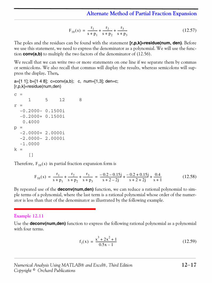
Numerical Analysis Using MATLAB® and Excel®, Third Edition 12−17Copyright © Orchard Publications
Alternate Method of Partial Fraction Expansion
(12.57)
The poles and the residues can be found with the statement [r,p,k]=residue(num, den). Beforewe use this statement, we need to express the denominator as a polynomial. We will use the func-tion conv(a,b) to multiply the two factors of the denominator of (12.56).
We recall that we can write two or more statements on one line if we separate them by commasor semicolons. We also recall that commas will display the results, whereas semicolons will sup-press the display. Then,
a=[1 1]; b=[1 4 8]; c=conv(a,b); c, num=[1,3]; den=c; [r,p,k]=residue(num,den)
c = 1 5 12 8r = -0.2000- 0.1500i -0.2000+ 0.1500i 0.4000 p = -2.0000+ 2.0000i -2.0000- 2.0000i -1.0000 k = []
Therefore, in partial fraction expansion form is
(12.58)
By repeated use of the deconv(num,den) function, we can reduce a rational polynomial to sim-ple terms of a polynomial, where the last term is a rational polynomial whose order of the numer-ator is less than that of the denominator as illustrated by the following example.
Example 12.11 Use the deconv(num,den) function to express the following rational polynomial as a polynomialwith four terms.
(12.59)
F10 s( )r1
s p1+--------------
r2s p2+--------------
r3s p3+--------------+ +=
F10 s( )
F10 s( )r1
s p1+--------------
r2
s p2+--------------
r3
s p3+--------------+ + 0.2– 0.15j–
s 2 2j–+------------------------------ 0.2– 0.15j+
s 2 2j+ +------------------------------ 0.4
s 1+-----------+ += =
f1 x( ) x3 2x2 1+ +0.5x 1–
-----------------------------=
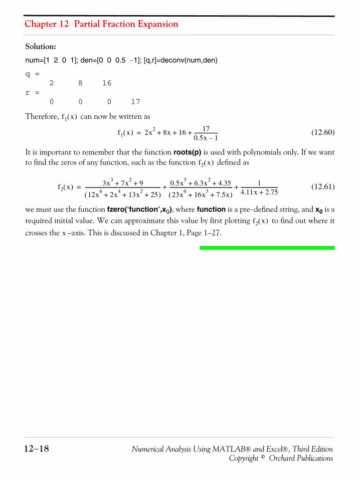
Chapter 12 Partial Fraction Expansion
12−18 Numerical Analysis Using MATLAB® and Excel®, Third EditionCopyright © Orchard Publications
Solution:
num=[1 2 0 1]; den=[0 0 0.5 −1]; [q,r]=deconv(num,den)
q = 2 8 16r = 0 0 0 17
Therefore, can now be written as
(12.60)
It is important to remember that the function roots(p) is used with polynomials only. If we wantto find the zeros of any function, such as the function defined as
(12.61)
we must use the function fzero(‘function’,x0), where function is a pre−defined string, and x0 is arequired initial value. We can approximate this value by first plotting to find out where itcrosses the −axis. This is discussed in Chapter 1, Page 1−27.
f1 x( )
f1 x( ) 2x2 8x 16 170.5x 1–-------------------+ + +=
f2 x( )
f2 x( ) 3x3 7x2 9+ +
12x6 2x4 13x2 25+ + +( )-------------------------------------------------------------- 0.5x5 6.3x2 4.35+ +
23x6 16x3 7.5x+ +( )---------------------------------------------------- 1
4.11x 2.75+------------------------------+ +=
f2 x( )
x
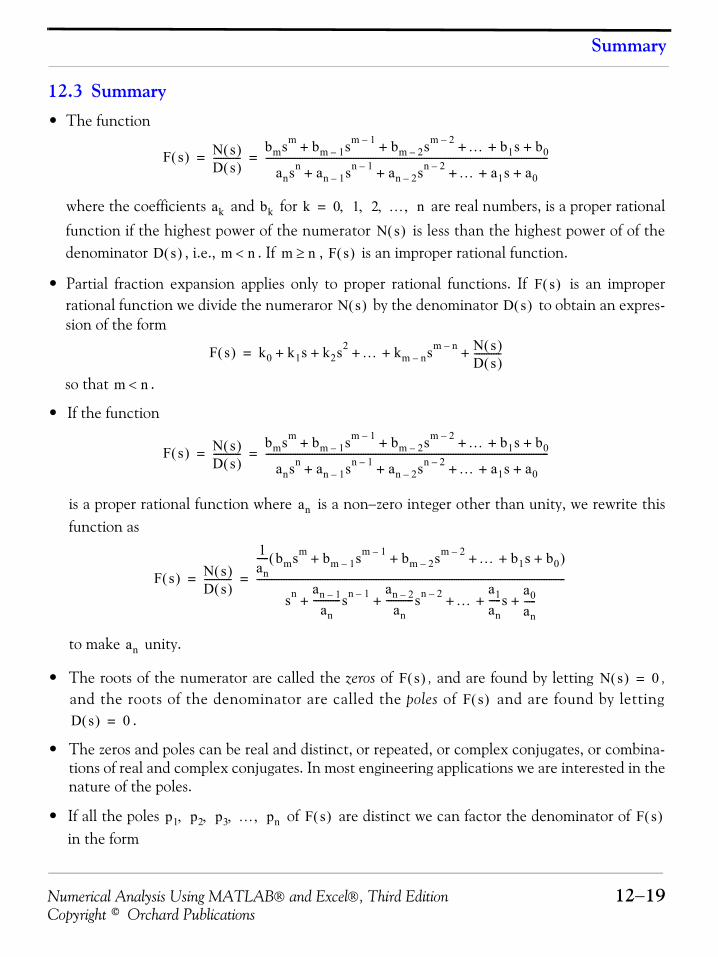
Numerical Analysis Using MATLAB® and Excel®, Third Edition 12−19Copyright © Orchard Publications
Summary
12.3 Summary• The function
where the coefficients and for are real numbers, is a proper rationalfunction if the highest power of the numerator is less than the highest power of of thedenominator , i.e., . If , is an improper rational function.
• Partial fraction expansion applies only to proper rational functions. If is an improperrational function we divide the numeraror by the denominator to obtain an expres-sion of the form
so that .
• If the function
is a proper rational function where is a non−zero integer other than unity, we rewrite thisfunction as
to make unity.
• The roots of the numerator are called the zeros of , and are found by letting ,and the roots of the denominator are called the poles of and are found by letting
.
• The zeros and poles can be real and distinct, or repeated, or complex conjugates, or combina-tions of real and complex conjugates. In most engineering applications we are interested in thenature of the poles.
• If all the poles of are distinct we can factor the denominator of in the form
F s( ) N s( )D s( )-----------
bmsm bm 1– sm 1– bm 2– sm 2– … b1s b0+ + + + +
ansn an 1– sn 1– an 2– sn 2– … a1s a0+ + + + +--------------------------------------------------------------------------------------------------------------------= =
ak bk k 0 1 2 … n, , , ,=
N s( )D s( ) m n< m n≥ F s( )
F s( )N s( ) D s( )
F s( ) k0 k1s k2s2 … km n– sm n– N s( )D s( )-----------+ + + + +=
m n<
F s( ) N s( )D s( )-----------
bmsm bm 1– sm 1– bm 2– sm 2– … b1s b0+ + + + +
ansn an 1– sn 1– an 2– sn 2– … a1s a0+ + + + +--------------------------------------------------------------------------------------------------------------------= =
an
F s( ) N s( )D s( )-----------
1an----- bmsm bm 1– sm 1– bm 2– sm 2– … b1s b0+ + + + +( )
sn an 1–
an-----------sn 1– an 2–
an-----------sn 2– …
a1an-----s
a0an-----+ + + + +
-------------------------------------------------------------------------------------------------------------------------------= =
an
F s( ) N s( ) 0=
F s( )D s( ) 0=
p1 p2 p3 … pn, , , , F s( ) F s( )
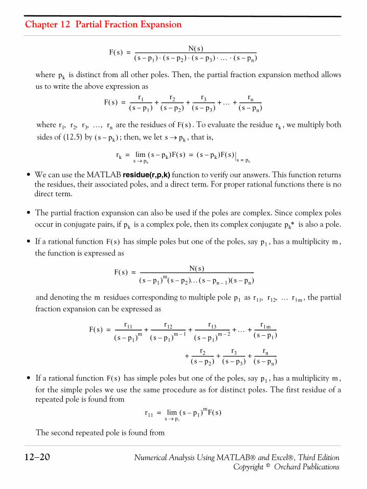
Chapter 12 Partial Fraction Expansion
12−20 Numerical Analysis Using MATLAB® and Excel®, Third EditionCopyright © Orchard Publications
where is distinct from all other poles. Then, the partial fraction expansion method allowsus to write the above expression as
where are the residues of . To evaluate the residue , we multiply bothsides of (12.5) by ; then, we let , that is,
• We can use the MATLAB residue(r,p,k) function to verify our answers. This function returnsthe residues, their associated poles, and a direct term. For proper rational functions there is nodirect term.
• The partial fraction expansion can also be used if the poles are complex. Since complex polesoccur in conjugate pairs, if is a complex pole, then its complex conjugate is also a pole.
• If a rational function has simple poles but one of the poles, say , has a multiplicity ,the function is expressed as
and denoting the residues corresponding to multiple pole as , the partialfraction expansion can be expressed as
• If a rational function has simple poles but one of the poles, say , has a multiplicity ,for the simple poles we use the same procedure as for distinct poles. The first residue of arepeated pole is found from
The second repeated pole is found from
F s( ) N s( )s p1–( ) s p2–( ) s p3–( ) … s pn–( )⋅ ⋅ ⋅ ⋅
--------------------------------------------------------------------------------------------------=
pk
F s( )r1
s p1–( )------------------
r2s p2–( )
------------------r3
s p3–( )------------------ …
rns pn–( )
------------------+ + + +=
r1 r2 r3 … rn, , , , F s( ) rk
s pk–( ) s pk→
rk s pk–( )F s( )s pk→lim s pk–( )F s( )
s pk== =
pk pk∗
F s( ) p1 m
F s( ) N s( )
s p1–( )m s p2–( )… s pn 1––( ) s pn–( )--------------------------------------------------------------------------------------------=
m p1 r11 r12 … r1m, ,
F s( )r11
s p1–( )m----------------------
r12
s p1–( )m 1–----------------------------
r13
s p1–( )m 2–---------------------------- …
r1ms p1–( )
------------------+ + + +=
r2
s p2–( )------------------
r3s p3–( )
------------------rn
s pn–( )------------------+ + +
F s( ) p1 m
r11 s p1–( )mF s( )s p1→lim=
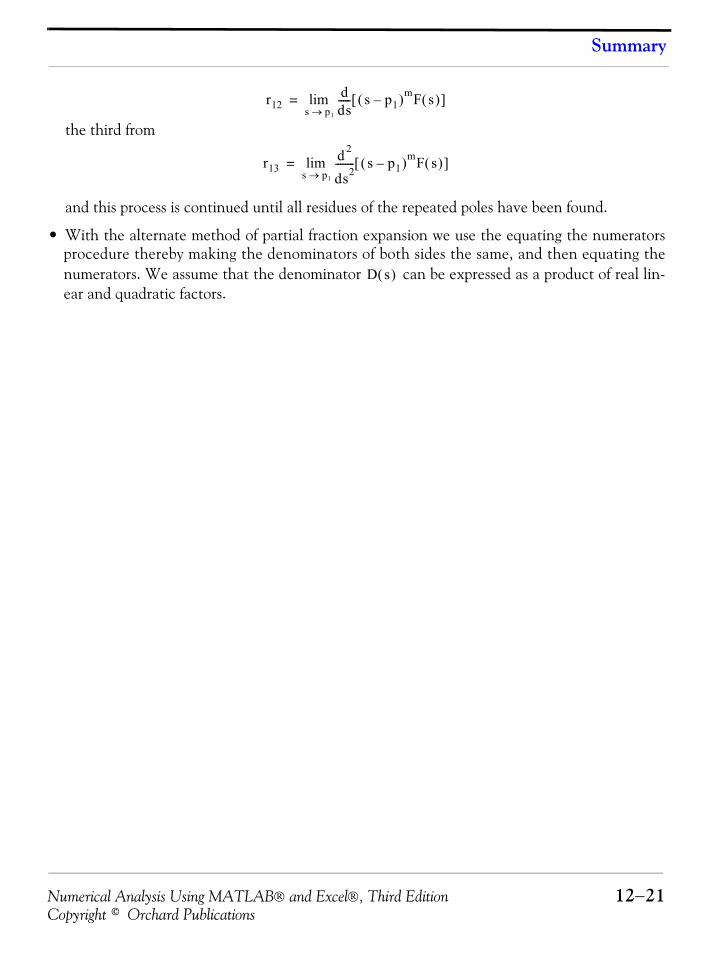
Numerical Analysis Using MATLAB® and Excel®, Third Edition 12−21Copyright © Orchard Publications
Summary
the third from
and this process is continued until all residues of the repeated poles have been found.
• With the alternate method of partial fraction expansion we use the equating the numeratorsprocedure thereby making the denominators of both sides the same, and then equating thenumerators. We assume that the denominator can be expressed as a product of real lin-ear and quadratic factors.
r12dds-----
s p1→lim s p1–( )mF s( )[ ]=
r13d 2
ds2--------
s p1→lim s p1–( )mF s( )[ ]=
D s( )
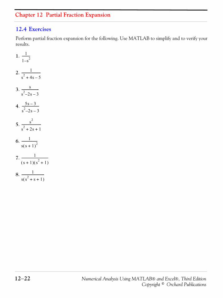
Chapter 12 Partial Fraction Expansion
12−22 Numerical Analysis Using MATLAB® and Excel®, Third EditionCopyright © Orchard Publications
12.4 ExercisesPerform partial fraction expansion for the following. Use MATLAB to simplify and to verify yourresults.
1.
2.
3.
4.
5.
6.
7.
8.
11 s2–-----------
1s2 4s 5–+-------------------------
ss2 2– s 3–-----------------------
5s 3–
s2 2– s 3–-----------------------
s2
s2 2s 1+ +--------------------------
1s s 1+( )2---------------------
1s 1+( ) s2 1+( )
-----------------------------------
1s s2 s 1+ +( )------------------------------
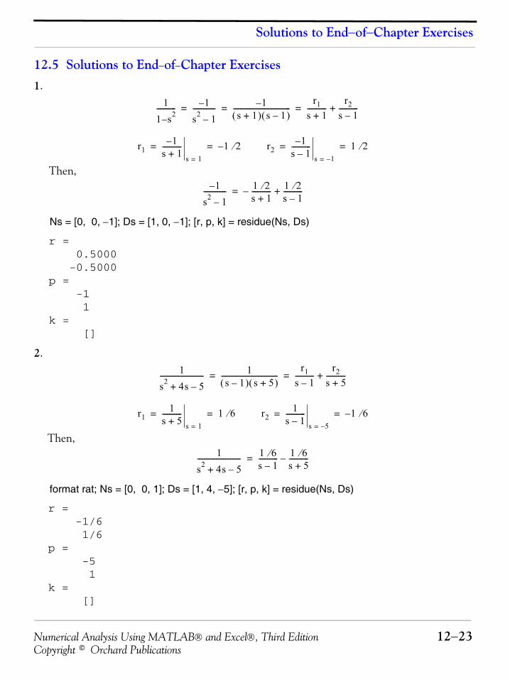
Numerical Analysis Using MATLAB® and Excel®, Third Edition 12−23Copyright © Orchard Publications
Solutions to End−of−Chapter Exercises
12.5 Solutions to End−of−Chapter Exercises1.
Then,
Ns = [0, 0, −1]; Ds = [1, 0, −1]; [r, p, k] = residue(Ns, Ds)
r = 0.5000 -0.5000p = -1 1k = []
2.
Then,
format rat; Ns = [0, 0, 1]; Ds = [1, 4, −5]; [r, p, k] = residue(Ns, Ds)
r = -1/6 1/6 p = -5 1 k = []
11 s2–----------- 1–
s2 1–------------- 1–
s 1+( ) s 1–( )---------------------------------
r1s 1+-----------
r2s 1–-----------+= = =
r11–
s 1+-----------
s 1=
1– 2⁄= = r21–
s 1–-----------
s 1–=
1 2⁄= =
1–
s2 1–------------- 1 2⁄
s 1+-----------– 1 2⁄
s 1–-----------+=
1s2 4s 5–+------------------------- 1
s 1–( ) s 5+( )---------------------------------
r1s 1–-----------
r2s 5+-----------+= =
r11
s 5+-----------
s 1=
1 6⁄= = r21
s 1–-----------
s 5–=
1– 6⁄= =
1s2 4s 5–+------------------------- 1 6⁄
s 1–----------- 1 6⁄
s 5+-----------–=

Chapter 12 Partial Fraction Expansion
12−24 Numerical Analysis Using MATLAB® and Excel®, Third EditionCopyright © Orchard Publications
3.
Then,
format rat; Ns = [0, 1, 0]; Ds = [1, −2, −3]; [r, p, k] = residue(Ns, Ds)
r = 3/4 1/4 p = 3 -1 k = []
4.
Then,
Ns = [0, 5, −3]; Ds = [1, −2, −3]; [r, p, k] = residue(Ns, Ds)
r = 3 2 p = 3 -1 k = []
ss2 2– s 3–----------------------- s
s 1+( ) s 3–( )---------------------------------
r1s 1+-----------
r2s 3–-----------+= =
r1s
s 3–-----------
s 1–=
1 4⁄= = r2s
s 1+-----------
s 3=
3 4⁄= =
ss2 2– s 3–----------------------- 1 4⁄
s 1+----------- 3 4⁄
s 3–-----------+=
5s 3–
s2 2– s 3–----------------------- 5s 3–
s 1+( ) s 3–( )---------------------------------
r1s 1+-----------
r2s 3–-----------+= =
r15s 3–s 3–
--------------s 1–=
2= = r25s 3–s 1+--------------
s 3=
3= =
5s 3–
s2 2– s 3–----------------------- 2
s 1+----------- 3
s 3–-----------+=
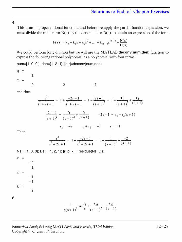
Numerical Analysis Using MATLAB® and Excel®, Third Edition 12−25Copyright © Orchard Publications
Solutions to End−of−Chapter Exercises
5.This is an improper rational function, and before we apply the partial fraction expansion, wemust divide the numeraror by the denominator to obtain an expression of the form
We could perform long division but we will use the MATLAB deconv(num,den) function toexpress the following rational polynomial as a polynomial with four terms.
num=[1 0 0 ]; den=[1 2 1]; [q,r]=deconv(num,den)
q = 1 r = 0 -2 -1
and thus
Then,
Ns = [1, 0, 0]; Ds = [1, 2, 1]; [r, p, k] = residue(Ns, Ds)
r = -2 1 p = -1 -1 k = 1
6.
N s( ) D s( )
F s( ) k0 k1s k2s2 … km n– sm n– N s( )D s( )-----------+ + + + +=
s2
s2 2s 1+ +-------------------------- 1 2– s 1–
s2 2s 1+ +--------------------------+ 1 2s 1+
s 1+( )2------------------– 1
r1
s 1+( )2------------------
r2s 1+( )
----------------+–= = =
2– s 1–
s 1+( )2------------------
r1
s 1+( )2------------------
r2s 1+( )
----------------+= 2– s 1– r1 r2 s 1+( )+=
r2 2–= r1 r2+ 1–= r1 1=
s2
s2 2s 1+ +-------------------------- 1 2– s 1–
s2 2s 1+ +--------------------------+ 1 1
s 1+( )2------------------ 2–
s 1+( )----------------+ += =
1s s 1+( )2---------------------
r1s----
r21
s 1+( )2------------------
r22s 1+( )
----------------+ +=
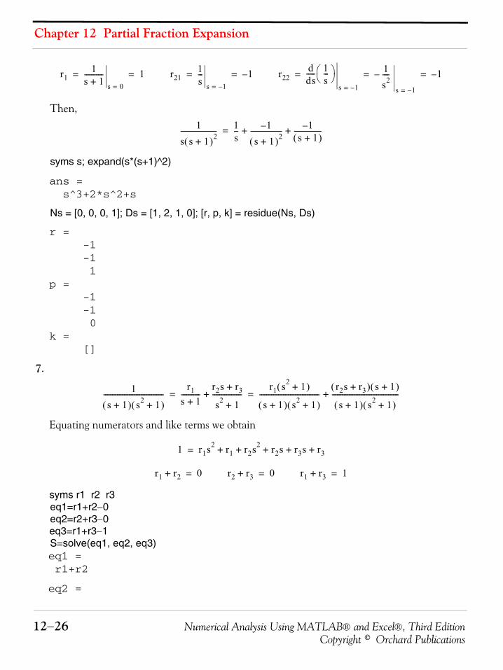
Chapter 12 Partial Fraction Expansion
12−26 Numerical Analysis Using MATLAB® and Excel®, Third EditionCopyright © Orchard Publications
Then,
syms s; expand(s*(s+1)^2)
ans = s^3+2*s^2+s
Ns = [0, 0, 0, 1]; Ds = [1, 2, 1, 0]; [r, p, k] = residue(Ns, Ds)
r = -1 -1 1 p = -1 -1 0 k = []
7.
Equating numerators and like terms we obtain
syms r1 r2 r3eq1=r1+r2−0eq2=r2+r3−0eq3=r1+r3−1S=solve(eq1, eq2, eq3)eq1 = r1+r2
eq2 =
r11
s 1+-----------
s 0=
1= = r211s---
s 1–=
1–= = r22dds----- 1
s---⎝ ⎠
⎛ ⎞
s 1–=
1s2----–
s 1–=
1–= = =
1s s 1+( )2--------------------- 1
s--- 1–
s 1+( )2------------------ 1–
s 1+( )----------------+ +=
1s 1+( ) s2 1+( )
-----------------------------------r1
s 1+-----------
r2s r3+
s2 1+-----------------+
r1 s2 1+( )
s 1+( ) s2 1+( )-----------------------------------
r2s r3+( ) s 1+( )
s 1+( ) s2 1+( )---------------------------------------+= =
1 r1s2 r1+ r2s2 r2s r3+ + s r3++=
r1 r2+ 0= r2 r3+ 0= r1 r3+ 1=
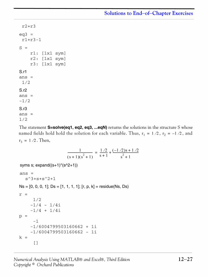
Numerical Analysis Using MATLAB® and Excel®, Third Edition 12−27Copyright © Orchard Publications
Solutions to End−of−Chapter Exercises
r2+r3
eq3 = r1+r3-1
S = r1: [1x1 sym] r2: [1x1 sym] r3: [1x1 sym]
S.r1ans = 1/2
S.r2ans =-1/2
S.r3ans =1/2
The statement S=solve(eq1, eq2, eq3, ...eqN) returns the solutions in the structure S whosenamed fields hold hold the solution for each variable. Thus, , , and
. Then,
syms s; expand((s+1)*(s^2+1))
ans = s^3+s+s^2+1
Ns = [0, 0, 0, 1]; Ds = [1, 1, 1, 1]; [r, p, k] = residue(Ns, Ds)
r = 1/2 -1/4 - 1/4i -1/4 + 1/4i p = -1 -1/6004799503160662 + 1i -1/6004799503160662 - 1i k = []
r1 1 2⁄= r2 1– 2⁄=
r3 1 2⁄=
1s 1+( ) s2 1+( )
----------------------------------- 1 2⁄s 1+----------- 1 2⁄–( )s 1 2⁄+
s2 1+-------------------------------------+=
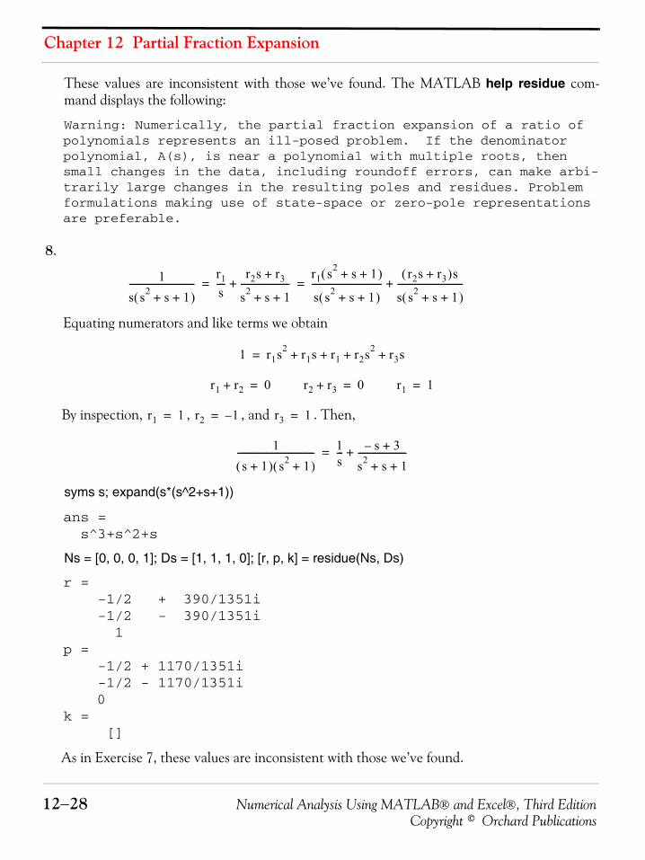
Chapter 12 Partial Fraction Expansion
12−28 Numerical Analysis Using MATLAB® and Excel®, Third EditionCopyright © Orchard Publications
These values are inconsistent with those we’ve found. The MATLAB help residue com-mand displays the following:
Warning: Numerically, the partial fraction expansion of a ratio of polynomials represents an ill-posed problem. If the denominator polynomial, A(s), is near a polynomial with multiple roots, then small changes in the data, including roundoff errors, can make arbi-trarily large changes in the resulting poles and residues. Problem formulations making use of state-space or zero-pole representations are preferable.
8.
Equating numerators and like terms we obtain
By inspection, , , and . Then,
syms s; expand(s*(s^2+s+1))
ans = s^3+s^2+s
Ns = [0, 0, 0, 1]; Ds = [1, 1, 1, 0]; [r, p, k] = residue(Ns, Ds)
r = -1/2 + 390/1351i -1/2 - 390/1351i 1 p = -1/2 + 1170/1351i -1/2 - 1170/1351i
0 k = []
As in Exercise 7, these values are inconsistent with those we’ve found.
1s s2 s 1+ +( )------------------------------
r1s----
r2s r3+
s2 s 1+ +----------------------+
r1 s2 s 1+ +( )
s s2 s 1+ +( )--------------------------------
r2s r3+( )s
s s2 s 1+ +( )------------------------------+= =
1 r1s2 r1s r1+ + r2s2 r3+ s+=
r1 r2+ 0= r2 r3+ 0= r1 1=
r1 1= r2 1–= r3 1=
1s 1+( ) s2 1+( )
----------------------------------- 1s--- s– 3+
s2 s 1+ +----------------------+=
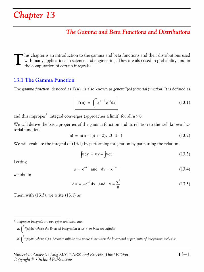
Numerical Analysis Using MATLAB® and Excel®, Third Edition 13−1Copyright © Orchard Publications
Chapter 13
The Gamma and Beta Functions and Distributions
his chapter is an introduction to the gamma and beta functions and their distributions usedwith many applications in science and engineering. They are also used in probability, and inthe computation of certain integrals.
13.1 The Gamma Function
The gamma function, denoted as , is also known as generalized factorial function. It is defined as
(13.1)
and this improper* integral converges (approaches a limit) for all .
We will derive the basic properties of the gamma function and its relation to the well known fac-torial function
(13.2)
We will evaluate the integral of (13.1) by performing integration by parts using the relation
(13.3)
Letting
(13.4)we obtain
(13.5)
Then, with (13.3), we write (13.1) as
* Improper integrals are two types and these are:
a. where the limits of integration or or both are infinite
b. where becomes infinite at a value between the lower and upper limits of integration inclusive.
T
Γ n( )
Γ n( ) xn 1– e x– xd0
∞
∫=
n 0>
f x( ) xda
b
∫ a b
f x( ) xda
b
∫ f x( ) x
n! n n 1–( ) n 2–( )…3 2 1⋅ ⋅=
u vd∫ uv v ud∫–=
u e x– and dv xn 1–==
du e x–– dx and v xn
n-----==
Chapter 13 The Gamma and Beta Functions and Distributions
13−2 Numerical Analysis Using MATLAB® and Excel®, Third EditionCopyright © Orchard Publications
(13.6)
With the condition that , the first term on the right side of (13.6) vanishes at the lower limit,that is, for . It also vanishes at the upper limit as . This can be proved with L’ Hôpi-tal’s rule* by differentiating both numerator and denominator times, where .Then,
(13.7)
Therefore, (13.6) reduces to
(13.8)
and with (13.1) we have
(13.9)
By comparing the two integrals of (13.9), we observe that
(13.10)
or
(13.11)
* Quite often, the ratio of two functions, such as , for some value of , say , results in the indeterminate form
. To work around this problem, we consider the limit , and we wish to find this limit, if it exists. L’Hôpi-
tal’s rule states that if , and if the limit as approaches exists, then,
Γ n( ) xne x–
n-------------
x 0=
∞1n--- xne x– xd
0
∞
∫+=
n 0>x 0= x ∞→
m m n≥
f x( )g x( )----------- x a
f a( )g a( )---------- 0
0---= f x( )
g x( )-----------
x a→lim
f a( ) g a( ) 0= = ddx------f x( ) d
dx------g x( )⁄ x a
f x( )g x( )-----------
x a→lim d
dx------f x( ) d
dx------g x( )⁄⎝ ⎠
⎛ ⎞x a→lim=
xne x–
n-------------
x ∞→lim xn
nex--------
x ∞→lim xm
m
d
d xn
xm
m
d
d nex-------------------
x ∞→lim xm 1–
m 1–
d
d nxn 1–
xm 1–
m 1–
d
d nex
------------------------------------x ∞→lim …= = = =
n n 1–( ) n 2–( )… n m– 1+( )xn m–
nex-------------------------------------------------------------------------------------
x ∞→lim=
n 1–( ) n 2–( )… n m– 1+( )
xm n– ex
--------------------------------------------------------------------x ∞→lim 0==
Γ n( ) 1n--- xne x– xd
0
∞
∫=
Γ n( ) xn 1– e x– xd0
∞
∫1n--- xne x– xd
0
∞
∫= =
Γ n( ) Γ n 1+( )n
---------------------=
nΓ n( ) Γ n 1+( )=
Numerical Analysis Using MATLAB® and Excel®, Third Edition 13−3Copyright © Orchard Publications
The Gamma Function
It is convenient to use (13.10) for , and (13.11) for .
From (13.10), we see that becomes infinite as .
For , (13.1) yields
(13.12)
Thus, we have derived the important relation,
(13.13)
From the recurring relation of (13.11), we obtain
(13.14)
and in general
(13.15)
The formula of (13.15) is a very useful relation; it establishes the relationship between the function and the factorial .
We must remember that, whereas the factorial is defined only for zero (recall that )and positive integer values, the gamma function exists (is continuous) everywhere except at and negative integer numbers, that is, , and so on. For instance, when , we canfind in terms of , but if we substitute the numbers and so on in(13.11), we obtain values which are not consistent with the definition of the function, asdefined in that relation.
Stated in other words, the function is defined for all positive integers and positive fractional val-ues, and for all negative fractional, but not negative integer values.
We can use MATLAB’s gamma(n) function to plot versus . This is done with the scriptbelow which produces the plot shown in Figure 13.1.
n=−4: 0.05: 4; g=gamma(n); plot(n,g); axis([−4 4 −6 6]); grid;title('The Gamma Function'); xlabel('n'); ylabel('Gamma(n)')
Figure 13.1 shows the plot of the function versus .
n 0< n 0>
Γ n( ) n 0→
n 1=
Γ 1( ) e x– xd0
∞
∫ e x–0
∞– 1= = =
Γ 1( ) 1=
Γ 2( ) 1 Γ⋅ 1( ) 1= =
Γ 3( ) 2 Γ⋅ 2( ) 2 1⋅ 2!= = =
Γ 4( ) 3 Γ⋅ 3( ) 3 2⋅ 3!= = =
Γ n 1+( ) n! for n 1 2 3 …, , ,= =
Γ n( )n!
n! 0! 1=
01 2 3–,–,– n 0.5–=
Γ 0.5–( ) Γ 0.5( ) 0 1 2 3–,–,–,Γ n( )
Γ n( )
Γ n( ) n
Γ n( ) n
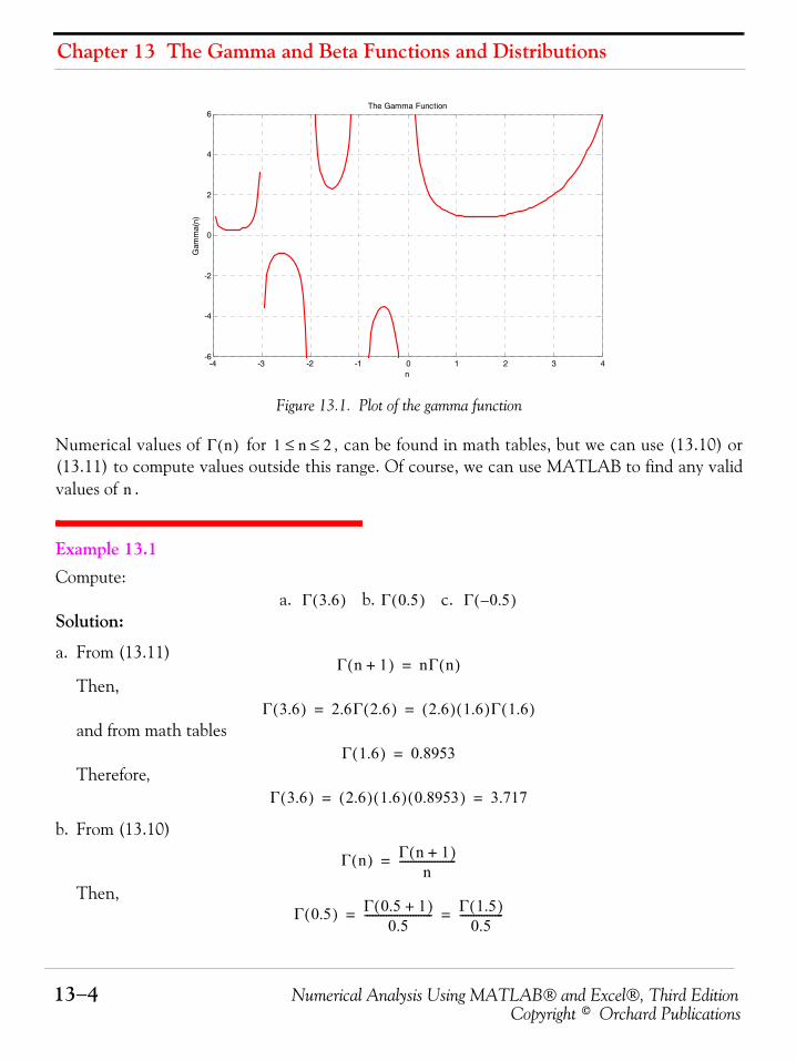
Chapter 13 The Gamma and Beta Functions and Distributions
13−4 Numerical Analysis Using MATLAB® and Excel®, Third EditionCopyright © Orchard Publications
Figure 13.1. Plot of the gamma function
Numerical values of for , can be found in math tables, but we can use (13.10) or(13.11) to compute values outside this range. Of course, we can use MATLAB to find any validvalues of .
Example 13.1 Compute:
a. b. c. Solution:
a. From (13.11)
Then,
and from math tables
Therefore,
b. From (13.10)
Then,
-4 -3 -2 -1 0 1 2 3 4-6
-4
-2
0
2
4
6The Gamma Function
n
Gam
ma(
n)
Γ n( ) 1 n 2≤ ≤
n
Γ 3.6( ) Γ 0.5( ) Γ 0.5–( )
Γ n 1+( ) nΓ n( )=
Γ 3.6( ) 2.6Γ 2.6( ) 2.6( ) 1.6( )Γ 1.6( )= =
Γ 1.6( ) 0.8953=
Γ 3.6( ) 2.6( ) 1.6( ) 0.8953( ) 3.717= =
Γ n( ) Γ n 1+( )n
---------------------=
Γ 0.5( ) Γ 0.5 1+( )0.5
------------------------- Γ 1.5( )0.5
----------------= =
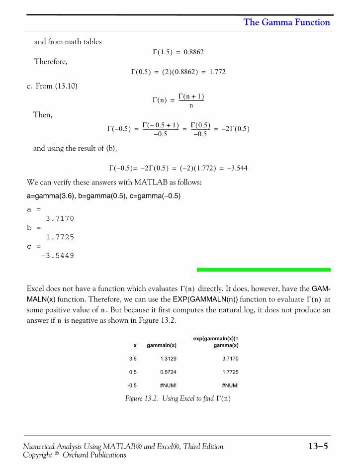
Numerical Analysis Using MATLAB® and Excel®, Third Edition 13−5Copyright © Orchard Publications
The Gamma Function
and from math tables
Therefore,
c. From (13.10)
Then,
and using the result of (b),
We can verify these answers with MATLAB as follows:
a=gamma(3.6), b=gamma(0.5), c=gamma(−0.5)
a = 3.7170b = 1.7725c = -3.5449
Excel does not have a function which evaluates directly. It does, however, have the GAM-MALN(x) function. Therefore, we can use the EXP(GAMMALN(n)) function to evaluate atsome positive value of . But because it first computes the natural log, it does not produce ananswer if is negative as shown in Figure 13.2.
Figure 13.2. Using Excel to find
Γ 1.5( ) 0.8862=
Γ 0.5( ) 2( ) 0.8862( ) 1.772= =
Γ n( ) Γ n 1+( )n
---------------------=
Γ 0.5–( ) Γ 0.5– 1+( )0.5–
------------------------------ Γ 0.5( )0.5–
---------------- 2Γ 0.5( )–= = =
Γ 0.5–( ) 2– Γ 0.5( )= 2–( ) 1.772( ) 3.544–= =
Γ n( )Γ n( )
nn
exp(gammaln(x))=x gammaln(x) gamma(x)
3.6 1.3129 3.7170
0.5 0.5724 1.7725
-0.5 #NUM! #NUM!
Γ n( )
Chapter 13 The Gamma and Beta Functions and Distributions
13−6 Numerical Analysis Using MATLAB® and Excel®, Third EditionCopyright © Orchard Publications
Example 13.2
Prove that when is a positive integer, the relation
(13.16)
is true.
Proof:
From (13.11),(13.17)
Then,(13.18)
Next, replacing n with on the left side of (13.18), we obtain
(13.19)
Substitution of (13.19) into (13.18) yields
(13.20)
By repeated substitutions, we obtain
(13.21)
and since , we have
(13.22)or
(13.23)
Example 13.3
Use the definition of the function to compute the exact value of
Solution:
From (13.1),
(13.24)
Then,
(13.25)
n
Γ n( ) n 1–( )!=
Γ n 1+( ) nΓ n( )=
Γ n( ) n 1–( )Γ n 1–( )=
n 1–
Γ n 1–( ) n 2–( )Γ n 2–( )=
Γ n( ) n 1–( ) n 2–( )Γ n 2–( )=
n
Γ n( ) n 1–( ) n 2–( ) n 3–( )…1Γ 1( )=
Γ 1( ) 1=
Γ n( ) n 1–( ) n 2–( ) n 3–( )…1=
Γ n( ) n 1–( )!=
Γ n( ) Γ 1 2⁄( )
Γ n( ) xn 1– e x– xd0
∞
∫=
Γ 12---⎝ ⎠
⎛ ⎞ x0.5 1– e x– xd0
∞
∫ x 0.5– e x– xd0
∞
∫= =
Numerical Analysis Using MATLAB® and Excel®, Third Edition 13−7Copyright © Orchard Publications
The Gamma Function
Letting
we obtain
or
By substitution of the last three relations into (13.25), we obtain
(13.26)
Next, we define as a function of both and , that is, we let
(13.27)
(13.28)
Multiplication of (13.27) by (13.28) yields
(13.29)
Now, we convert (13.29) to polar coordinates by making the substitution
(13.30)
and by recalling that:
1. the total area of a region is found by either one of the double integrals
(13.31)
2. from differential calculus
(13.32)
Then,
(13.33)
We observe that as ,
x y2=
dxdy------ 2y=
dx 2ydy=
Γ 12---⎝ ⎠
⎛ ⎞ y2 0.5–( )e y2– 2ydy0
∞
∫ 2 y 1– ye y2– dy0
∞
∫ 2 e y2– dy0
∞
∫= = =
Γ 1 2⁄( ) x y
Γ 12---⎝ ⎠
⎛ ⎞ 2 e x2– dx0
∞
∫=
Γ 12---⎝ ⎠
⎛ ⎞ 2 e y2– dy0
∞
∫=
Γ 12---⎝ ⎠
⎛ ⎞ 24 e x2– dx e y2– dy
0
∞
∫0
∞
∫ 4 e x2 y2+( )– xd yd0
∞
∫0
∞
∫= =
ρ2 x2 y2+=
A xd yd∫∫ r rd θd∫∫= =
ddu------eu2
eu2 ddu------u2 2ueu2
= =
ρe ρ2– ρdρ1
ρ2
∫ 12---– e ρ2–=
x ∞ and y ∞→→
Chapter 13 The Gamma and Beta Functions and Distributions
13−8 Numerical Analysis Using MATLAB® and Excel®, Third EditionCopyright © Orchard Publications
(13.34)
Substitution of (13.30), (13.33) and (13.34) into (13.29) yields
and thus, we have obtained the exact value
(13.35)
Example 13.4 Compute:
a. b . c. Solution:
Using the relations
we obtain:
a. for ,
b. for ,
c. for ,
Other interesting relations involving the function are:
(13.36)
(13.37)
ρ ∞ and θ π 2⁄ →→
Γ 12---⎝ ⎠
⎛ ⎞ 22– e ρ2–
ρ 0=
∞
⎝ ⎠⎛ ⎞ θd
0
π 2⁄
∫ 2– 0 1–( ) θd0
π 2⁄
∫ 2 θd0
π 2⁄
∫ 2θ 0π 2⁄ π= = = = =
Γ 12---⎝ ⎠
⎛ ⎞ π=
Γ 0.5–( ) Γ 1.5–( ) Γ 2.5–( )
Γ n( ) Γ n 1+( )n
---------------------- and Γ 0.5( ) π==
n 0.5–=
Γ 0.5–( ) Γ 0.5( )0.5–
----------------- π0.5–
---------- 2 π–= = =
n 1.5–=
Γ 1.5–( ) Γ 1.5– 1+( )1.5–
------------------------------- Γ 0.5–( )1.5–
-------------------- 2 π–1.5–
-------------- 43--- π= = = =
n 2.5–=
Γ 2.5–( ) Γ 2.5– 1+( )2.5–
------------------------------- Γ 1.5–( )2.5–
--------------------
43--- π
2.5–----------- 8
15------– π= = = =
Γ n( )
Γ n( )Γ 1 n–( ) πnπsin
--------------=
for 0 n 1< <
22n 1– Γ n( )Γ n 12---+⎝ ⎠
⎛ ⎞ πΓ 2n( )=
for any n negative integer≠
Numerical Analysis Using MATLAB® and Excel®, Third Edition 13−9Copyright © Orchard Publications
The Gamma Function
(13.38)
Relation (13.38) is referred to as Stirling’s asymptotic series for the function. If is a positiveinteger, the factorial can be approximated as
(13.39)
Example 13.5 Use (13.36) to prove that
Proof:
or
Therefore,
Example 13.6 Compute the product
Solution:
Using (13.36), we obtain
or
Γ n 1+( ) n!=
2πnnne n– 1 112n--------- 1
288n2-------------- 139
51840n3-------------------- 571
2488320n4--------------------------–– …+ + +
⎩ ⎭⎨ ⎬⎧ ⎫
=
Γ n( ) nn!
n! 2πnnne n–≈
Γ 12---⎝ ⎠
⎛ ⎞ π=
Γ 12---⎝ ⎠
⎛ ⎞Γ 1 12---–⎝ ⎠
⎛ ⎞ Γ 12---⎝ ⎠
⎛ ⎞Γ 12---⎝ ⎠
⎛ ⎞ ππ2---sin
-----------= =
Γ 12---⎝ ⎠
⎛ ⎞ 2π=
Γ 12---⎝ ⎠
⎛ ⎞ π=
Γ 13---⎝ ⎠
⎛ ⎞Γ 23---⎝ ⎠
⎛ ⎞
Γ 13---⎝ ⎠
⎛ ⎞Γ 1 13---–⎝ ⎠
⎛ ⎞ ππ3---sin
-----------=
Chapter 13 The Gamma and Beta Functions and Distributions
13−10 Numerical Analysis Using MATLAB® and Excel®, Third EditionCopyright © Orchard Publications
Example 13.7 Use (13.37) to find
Solution:
Example 13.8
Use (13.39) to compute
Solution:
We use MATLAB as a calculator, that is, we type and execute the expression
sqrt(2*pi*50)*50^50*exp(−50)
ans = 3.0363e+064
This is an approximation. To find the exact value, we use the relation and theMATLAB gamma(n) function. Then,
gamma(50+1)
ans = 3.0414e+064
We can check this answer with the Excel FACT(n) function, that is,
=FACT(50) and Excel displays 3.04141E+64
Γ 13---⎝ ⎠
⎛ ⎞Γ 23---⎝ ⎠
⎛ ⎞ π3 2⁄
-------------- 2π3
------- 2 3π3
-------------= = =
Γ 32---⎝ ⎠
⎛ ⎞
23 1– Γ 32---⎝ ⎠
⎛ ⎞Γ 32--- 1
2---+⎝ ⎠
⎛ ⎞ πΓ 2 32---⋅⎝ ⎠
⎛ ⎞=
22Γ 32---⎝ ⎠
⎛ ⎞Γ 2( ) πΓ 3( )=
Γ 32---⎝ ⎠
⎛ ⎞ πΓ 3( )4Γ 2( )
------------------- 2! π4 1⋅------------ π
2------= = =
50!
50! 2π 50× 50×50
e 50–×≈
Γ n 1+( ) n!=
Numerical Analysis Using MATLAB® and Excel®, Third Edition 13−11Copyright © Orchard Publications
The Gamma Function
The function is very useful in integrating some improper integrals. Some examples follow.
Example 13.9
Using the definition of the function, evaluate the integrals
a. b.
Solution:
By definition,
Then,a.
b.Let ; then, , and by substitution,
Example 13.10
A negatively charged particle is meters apart from the positively charged side of an electricfield. It is initially at rest, and then moves towards the positively charged side with a forceinversely proportional to its distance from it. Assuming that the particle moves towards the cen-ter of the positively charged side, considered to be the center of attraction , derive an expres-sion for the time required the negatively charged particle to reach in terms of the distance and its mass .
Solution:
Let the center of attraction be the point zero on the −axis, as indicated in Figure 13.3.
Γ n( )
Γ n( )
x4e x– xd0
∞
∫ x5e 2x– xd0
∞
∫
xn 1– e x– xd0
∞
∫ Γ n( )=
x4e x– xd0
∞
∫ Γ 5( ) 4! 24= = =
2x y= dx dy 2⁄=
x5e 2x– xd0
∞
∫y2---⎝ ⎠
⎛ ⎞ 5e y– yd
2------
0
∞
∫126----- y5e y– yd
0
∞
∫= =
Γ 6( )64
----------- 5!64------ 120
64--------- 15
8------= = ==
α
00 α
m
0 x
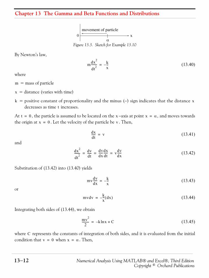
Chapter 13 The Gamma and Beta Functions and Distributions
13−12 Numerical Analysis Using MATLAB® and Excel®, Third EditionCopyright © Orchard Publications
Figure 13.3. Sketch for Example 13.10
By Newton’s law,
(13.40)
where
= mass of particle
= distance (varies with time)
= positive constant of proportionality and the minus (−) sign indicates that the distance decreases as time increases.
At , the particle is assumed to be located on the −axis at point , and moves towardsthe origin at . Let the velocity of the particle be . Then,
(13.41)
and
(13.42)
Substitution of (13.42) into (13.40) yields
(13.43)
or
(13.44)
Integrating both sides of (13.44), we obtain
(13.45)
where represents the constants of integration of both sides, and it is evaluated from the initialcondition that when . Then,
α0
movement of particlex
mdx2
dt2-------- k
x---–=
m
x
k xt
t 0= x x α=
x 0= v
dxdt------ v=
dx2
dt2-------- dv
dt------ dv
dx------dx
dt------ vdv
dx------= = =
mvdvdx------ k
x---–=
mvdv kx--- dx( )–=
mv2
2---------- k xln C+–=
Cv 0= x α=
Numerical Analysis Using MATLAB® and Excel®, Third Edition 13−13Copyright © Orchard Publications
The Gamma Function
(13.46)and by substitution into (13.45),
(13.47)
Solving for and taking the square root of both sides we obtain
(13.48)
Since decreases as increases, we choose the negative sign, that is,
(13.49)
Solving (13.49) for we obtain
(13.50)
We are interested in the time required for the particle to reach the origin . We denote thistime as ; it is found from the relation below, noting that the integration on the right side iswith respect to the distance x where at , , and at , . Then,
(13.51)
To simplify (13.51), we let
(13.52)
or
(13.53)Also, since
the lower and upper limits of integration in (13.51), are being replaced with and respec-tively. Therefore, we express (13.51) as
C k αln=
mv2
2---------- k αln k xln– k α
x---ln= =
v2
v dxdt------ 2k
m------ α
x---ln±= =
x t
dxdt------ 2k
m------ α
x---ln–=
dt
dt m2k------– dx
α x⁄( )ln-------------------------=
0T
t 0= x α= τ t= x 0=
T τd0
t
∫ m2k------– dx
α x⁄( )ln-------------------------
α
0
∫= =
y αx---⎝ ⎠
⎛ ⎞ then e y,ln αx---= =
x αe y– and dx, αe y– dy–= =
αx---⎝ ⎠
⎛ ⎞lnx α→lim 0 and α
x---⎝ ⎠
⎛ ⎞lnx 0→lim ∞==
0 ∞
Chapter 13 The Gamma and Beta Functions and Distributions
13−14 Numerical Analysis Using MATLAB® and Excel®, Third EditionCopyright © Orchard Publications
Finally, using the definition of the function, we obtain
(13.54)
Example 13.11 Evaluate the integrals
(13.55)
Solution:
From the definition of the function,
(13.56)
Also,
(13.57)
For and , multiplication of (13.56) by (13.57) yields
(13.58)
where and are dummy variables of integration. Next, letting and , we obtain and . Then, with these substitutions, relation (13.58) it written as
(13.59)
Next, we convert (13.59) to polar coordinates by letting and Then,
T m2k------– αe y– dy–
y---------------------
0
∞
∫ α m2k------ y 1 2⁄– e y– dy
0
∞
∫= =
Γ n( )
T αΓ 12---⎝ ⎠
⎛ ⎞ m2k------ α π m
2k------ α πm
2k--------= = =
θncos θd0
π 2⁄
∫ and θnsin θd0
π 2⁄
∫
Γ n( )
Γ n( ) xn 1– e x– xd0
∞
∫=
Γ m( ) xm 1– e x– xd0
∞
∫=
m 0> n 0>
Γ m( )Γ n( ) um 1– e u– ud0
∞
∫ vn 1– e v– vd0
∞
∫=
u v u x2= v y2=
du 2xdx= dv 2ydy=
Γ m( )Γ n( ) x2 m 1–( )2xe x2– xd
0
∞
∫ y2 n 1–( )2ye y2– yd
0
∞
∫ 4 x2m 2– xe x2– xd0
∞
∫ y2n 2– ye y2– yd0
∞
∫= =
4 x2m 1– y2n 1– e x2 y2+( )– xd yd0
∞
∫0
∞
∫=
x ρ θcos= y ρ θsin=
Numerical Analysis Using MATLAB® and Excel®, Third Edition 13−15Copyright © Orchard Publications
The Gamma Function
(13.60)
To simplify (13.60), we let ; then, and thus relation (13.60) is written as
(13.61)
Rearranging (13.61) we obtain
(13.62)
and this expression can be simplified by replacing with , that is, , and
with , that is, . Then, we obtain the special case of (13.62) as
(13.63)
If, in (13.62), we replace with and with , we obtain the integral of the function as
(13.64)
We observe that (13.63) and (13.64) are equal since and can be interchanged. Therefore,
(13.65)
Γ m( )Γ n( ) 4 ρ θcos( )2m 1– ρ θsin( )2n 1–
e ρ2– ρ ρd θd0
∞
∫0
π 2⁄
∫=
2 θ2m 1–cos θ2n 1–sin⋅ θd ρ2m 2n 2–+ eρ2–
2ρ ρd0
∞
∫0
π 2⁄
∫=
ρ2 w= dw 2ρdρ=
Γ m( )Γ n( ) 2 θ2m 1–cos θ2n 1–sin⋅ θd wm n 1–+ ew–
wd0
∞
∫0
π 2⁄
∫=
2 θ2m 1–cos θ2n 1–sin⋅ θ Γ m n+( )⋅d0
π 2⁄
∫=
θ2m 1–cos θ2n 1–sin⋅ θd0
π 2⁄
∫ Γ m( )Γ n( )2Γ m n+( )--------------------------=
2m 1– n m n 1+( )2
-----------------=
2n 1– 0 n 12---=
θncos θd0
π 2⁄
∫Γ n 1+
2------------⎝ ⎠
⎛ ⎞Γ 12---⎝ ⎠
⎛ ⎞
2Γ n 1+2
------------ 12---+⎝ ⎠
⎛ ⎞-------------------------------------------
Γ n 1+2
------------⎝ ⎠⎛ ⎞
Γ n2--- 1+⎝ ⎠
⎛ ⎞------------------------- π
2-------= =
2m 1– 0 2n 1– m θnsin
θmsin θd0
π 2⁄
∫Γ 1
2---⎝ ⎠
⎛ ⎞Γ m 1+2
--------------⎝ ⎠⎛ ⎞
2Γ 12--- m 1+
2--------------+⎝ ⎠
⎛ ⎞----------------------------------------------
Γ m 1+2
--------------⎝ ⎠⎛ ⎞
Γ m2---- 1+⎝ ⎠
⎛ ⎞--------------------------- π
2-------= =
m n
θncos θd0
π 2⁄
∫ θnsin θd0
π 2⁄
∫Γ n 1+
2------------⎝ ⎠
⎛ ⎞
Γ n2--- 1+⎝ ⎠
⎛ ⎞----------------------- π
2------- n 1–>= =
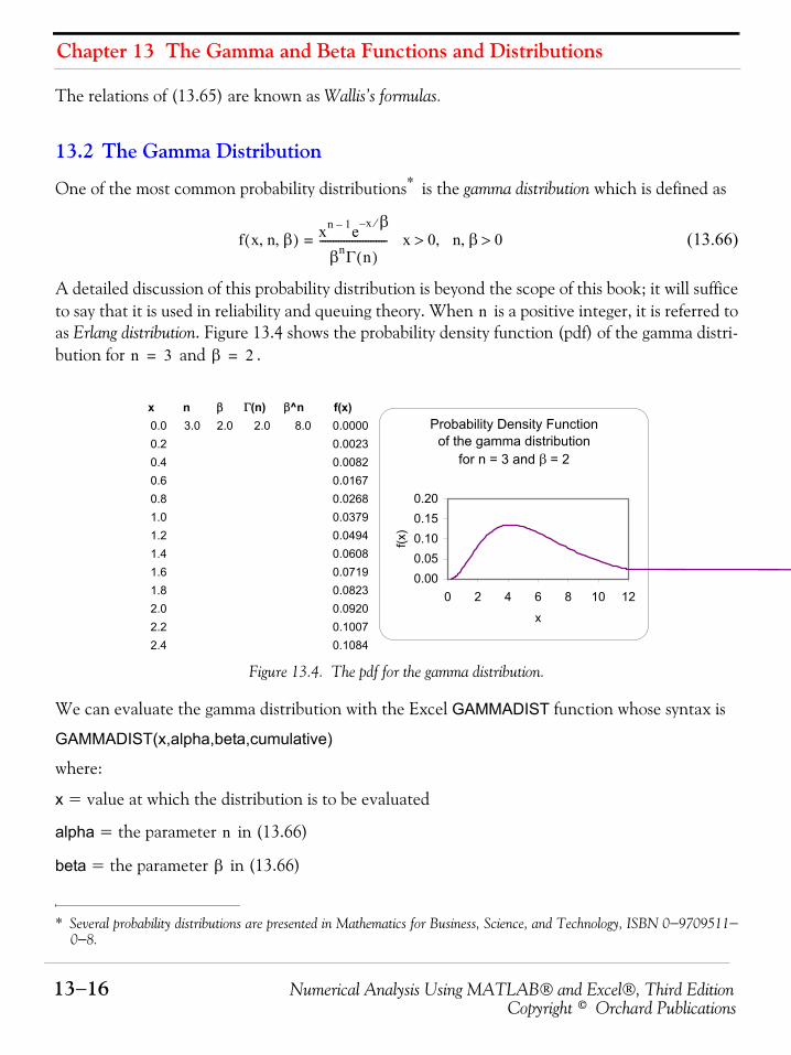
Chapter 13 The Gamma and Beta Functions and Distributions
13−16 Numerical Analysis Using MATLAB® and Excel®, Third EditionCopyright © Orchard Publications
The relations of (13.65) are known as Wallis’s formulas.
13.2 The Gamma Distribution
One of the most common probability distributions* is the gamma distribution which is defined as
(13.66)
A detailed discussion of this probability distribution is beyond the scope of this book; it will sufficeto say that it is used in reliability and queuing theory. When is a positive integer, it is referred toas Erlang distribution. Figure 13.4 shows the probability density function (pdf) of the gamma distri-bution for and .
Figure 13.4. The pdf for the gamma distribution.
We can evaluate the gamma distribution with the Excel GAMMADIST function whose syntax is
GAMMADIST(x,alpha,beta,cumulative)
where:
x = value at which the distribution is to be evaluated
alpha = the parameter in (13.66)
beta = the parameter in (13.66)
* Several probability distributions are presented in Mathematics for Business, Science, and Technology, ISBN 0−9709511−0−8.
f x n β, ,( ) xn 1– e x β⁄–
βnΓ n( )-------------------------= x 0 n β 0>,,>
n
n 3= β 2=
x n β Γ(n) β^n f(x)0.0 3.0 2.0 2.0 8.0 0.00000.2 0.00230.4 0.00820.6 0.01670.8 0.02681.0 0.03791.2 0.04941.4 0.06081.6 0.07191.8 0.08232.0 0.09202.2 0.10072.4 0.1084
Probability Density Functionof the gamma distribution
for n = 3 and β = 2
0.000.050.100.150.20
0 2 4 6 8 10 12
x
f(x)
n
β
Numerical Analysis Using MATLAB® and Excel®, Third Edition 13−17Copyright © Orchard Publications
The Beta Function
cumulative = a TRUE / FALSE logical value; if TRUE, GAMMADIST returns the cumulativedistribution function (cdf), and if FALSE, it returns the probability density function* (pdf).
Example 13.12
Use Excel’s GAMMADIST function to evaluate , that is, the pdf of the gamma distribution if:
a. , , and
b. , , and
Solution:
Since we are interested in the probability density function (pdf) values, we specify the FALSEcondition. Then,
a.=GAMMADIST(4,3,2,FALSE) returns 0.1353
b.=GAMMADIST(7,3,2,FALSE) returns 0.0925
We observe that these values are consistent with the plot of Figure 13.4.
13.3 The Beta Function
The beta function, denoted as , is defined as
(13.67)
where and .
Example 13.13 Prove that
(13.68)Proof:
Let ; then, . We observe that as , and as , . There-fore,
* Several probability density functions are also presented on the text mentioned on the footnote of the previous page.
f x( )
x 4= n 3= β 2=
x 7= n 3= β 2=
B m n,( )
B m n,( ) xm 1– 1 x–( )n 1– xd0
1
∫=
m 0> n 0>
B m n,( ) B n m,( )=
x 1 y–= dx dy–= x 0→ y 1→ x 1→ y 0→
Chapter 13 The Gamma and Beta Functions and Distributions
13−18 Numerical Analysis Using MATLAB® and Excel®, Third EditionCopyright © Orchard Publications
and thus (13.68) is proved.
Example 13.14 Prove that
(13.69)
Proof:
We let ; then, . We observe that as , and as ,. Then,
(13.70)
Example 13.15 Prove that
(13.71)
Proof:
The proof is evident from (13.62) and (13.70).
The function is also useful in evaluating certain integrals as illustrated by the followingexamples.
B m n,( ) xm 1– 1 x–( )n 1– xd0
1
∫ 1 y–( )m 1– 1 1 y–( )–[ ]n 1– yd1
0
∫–= =
1 y–( )m 1– yn 1– yd0
1
∫ yn 1– 1 y–( )m 1– yd0
1
∫ B n m,( )= ==
B m n,( ) 2 θ2m 1–cos θ2n 1–sin⋅ θd0
π 2⁄
∫=
x θ2sin= dx 2 θ θdθcossin= x 0→ θ 0→ x 1→θ π 2⁄→
B m n,( ) xm 1– 1 x–( )n 1– xd0
1
∫=
2 θ2sin( ) θ2cos( )m 1–
θ θ θdcossinn 1–
0
π 2⁄
∫=
2 θ2m 1–sin( ) θ2m 1–cos( ) θd0
π 2⁄
∫=
B m n,( ) Γ m( )Γ n( )Γ m n+( )-------------------------=
B m n,( )
Numerical Analysis Using MATLAB® and Excel®, Third Edition 13−19Copyright © Orchard Publications
The Beta Function
Example 13.16 Evaluate the integral
(13.72)
Solution:
By definition
and thus for this example,
Using (13.71) we obtain
(13.73)
We can also use MATLAB’s beta(m,n) function. For this example,
format rat; % display answer in rational formatz=beta(5,4)
z = 1/280
Excel does not have a function that computes the function directly. However, we canuse (13.71) for its computation as shown in Figure 13.5.
Figure 13.5. Computation of the beta function with Excel.
Example 13.17 Evaluate the integral
(13.74)
x4 1 x–( )3 xd0
1
∫
B m n,( ) xm 1– 1 x–( )n 1– xd0
1
∫=
x4 1 x–( )3 xd0
1
∫ B 5 4,( )=
B 5 4,( ) Γ 5( )Γ 4( )Γ 9( )
------------------------ 4!3!8!
---------- 24 6×40320--------------- 144
40320--------------- 1
280---------= = = = =
B m n,( )
p gΓ(m) Γ(n) Γ(m+n) Beta(m,n)=
exp(gammaln(m)) exp(gammaln(n)) exp(gammaln(m+n)) Γ(m) x Γ(n) / Γ(m+n)m= 5
24.00 6.00 40320.00 1/280n= 4
x2
2 x–---------------- xd
0
2
∫
Chapter 13 The Gamma and Beta Functions and Distributions
13−20 Numerical Analysis Using MATLAB® and Excel®, Third EditionCopyright © Orchard Publications
Solution:
Let ; then , and . We observe that as , , and as ,. Then, (13.74) becomes
(13.75)
where
(13.76)
Then, from (13.74), (13.75) and (13.76) we obtain
(13.77)
13.4 The Beta DistributionThe beta distribution is defined as
(13.78)
A plot of the beta probability density function (pdf) for and , is shown in Figure13.6.
As with the gamma probability distribution, a detailed discussion of the beta probability distribu-tion is beyond the scope of this book; it will suffice to say that it is used in computing variations inpercentages of samples such as the percentage of the time in a day people spent at work, drivinghabits, eating times and places, etc.
Using (13.71) we can express the beta distribution as
(13.79)
x 2v= x2 4v2= dx 2dv= x 0→ v 0→ x 2→v 1→
4v2
2 2v–-------------------2 vd
0
1
∫82
------- v2
1 v–---------------- vd
0
1
∫ 4 2 v2 1 v–( )1 2⁄–
vd0
1
∫==
4 2 B 3 12---,⎝ ⎠
⎛ ⎞⋅ 4 2 Γ 3( )Γ 1 2⁄( )Γ 7 2⁄( )
-------------------------------==
Γ 3( ) 2!=
Γ 1 2⁄( ) π=
Γ 7 2⁄( ) 7 2⁄ 1–( )Γ 7 2⁄ 1–( ) 5 2⁄( ) Γ 5 2⁄( ) 5 2⁄( ) 5 2⁄ 1–( )Γ 5 2⁄ 1–( )= = =
5 2⁄ 3 2⁄ 3 2⁄ 1–( )Γ 3 2⁄ 1–( )⋅ ⋅ 15 8⁄( )Γ 1 2⁄( ) 15 π 8⁄= ==
x2
2 x–---------------- xd
0
2
∫ 4 2 2! π⋅ ⋅15 π 8⁄
-------------------------------- 64 215
-------------= =
f x m n, ,( ) xm 1– 1 x–( )n 1–
B m n,( )---------------------------------------= x 0 1< m n 0>,,<
m 3= n 2=
f x m n, ,( ) Γ m n+( )Γ m( )Γ n( )------------------------- xm 1– 1 x–( )n 1– x 0 1< m n 0>,,<⋅=
Numerical Analysis Using MATLAB® and Excel®, Third Edition 13−21Copyright © Orchard Publications
The Beta Distribution
Figure 13.6. The pdf of the beta distribution
We can evaluate the beta cumulative distribution function (cdf) with Excels’s BETADIST func-tion whose syntax is
BETADIST(x,alpha,beta,A,B)
where:
x = value between A and B at which the distribution is to be evaluated
alpha = the parameter in (13.79)
beta = the parameter in (13.79)
A = the lower bound to the interval of x
B = the upper bound to the interval of x
From the plot of Figure 13.6, we see that when , which represents the probabil-ity density function, is zero. However, the cumulative distribution (the area under the curve) atthis point is or unity since this is the upper limit of the −range. This value can be verifiedby
=BETADIST(1,3,2,0,1) which returns 1.0000
x m n Γ(m) Γ(n) Γ(m+n) x(m-1) (1-x)(n-1) f(x,m,n)0.00 3.0 2.0 2.0 1.0 24.0 0.0000 1.0000 0.00000.02 0.0004 0.9800 0.00470.04 0.0016 0.9600 0.01840.06 0.0036 0.9400 0.04060.08 0.0064 0.9200 0.07070.10 0.0100 0.9000 0.10800.12 0.0144 0.8800 0.15210.14 0.0196 0.8600 0.20230.16 0.0256 0.8400 0.25800.18 0.0324 0.8200 0.31880.20 0.0400 0.8000 0.38400.22 0.0484 0.7800 0.45300.24 0.0576 0.7600 0.52530.26 0.0676 0.7400 0.60030.28 0.0784 0.7200 0.67740.30 0.0900 0.7000 0.75600.32 0.1024 0.6800 0.83560.34 0.1156 0.6600 0.9156
Probability Density Functionof the Beta Distribution
for m = 3 and n = 2
0.0
0.4
0.8
1.2
1.6
2.0
0.0 0.2 0.4 0.6 0.8 1.0
x
f(x,m
,n)
m
n
x 1= f x m n, ,( )
100% x
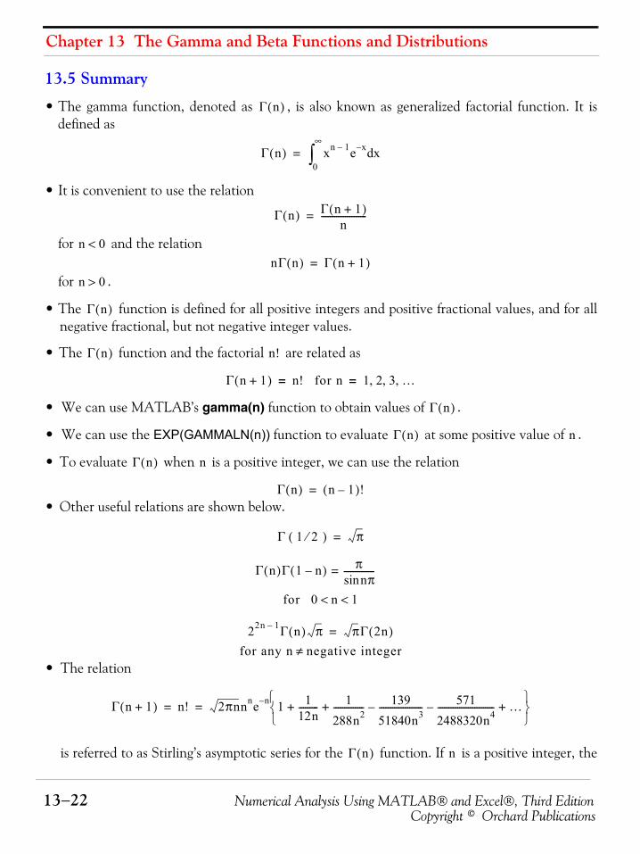
Chapter 13 The Gamma and Beta Functions and Distributions
13−22 Numerical Analysis Using MATLAB® and Excel®, Third EditionCopyright © Orchard Publications
13.5 Summary
• The gamma function, denoted as , is also known as generalized factorial function. It isdefined as
• It is convenient to use the relation
for and the relation
for .
• The function is defined for all positive integers and positive fractional values, and for allnegative fractional, but not negative integer values.
• The function and the factorial are related as
• We can use MATLAB’s gamma(n) function to obtain values of .
• We can use the EXP(GAMMALN(n)) function to evaluate at some positive value of .
• To evaluate when is a positive integer, we can use the relation
• Other useful relations are shown below.
• The relation
is referred to as Stirling’s asymptotic series for the function. If is a positive integer, the
Γ n( )
Γ n( ) xn 1– e x– xd0
∞
∫=
Γ n( ) Γ n 1+( )n
---------------------=
n 0<nΓ n( ) Γ n 1+( )=
n 0>
Γ n( )
Γ n( ) n!
Γ n 1+( ) n! for n 1 2 3 …, , ,= =
Γ n( )
Γ n( ) n
Γ n( ) n
Γ n( ) n 1–( )!=
Γ 1 2⁄( ) π=
Γ n( )Γ 1 n–( ) πnπsin
--------------=
for 0 n 1< <
22n 1– Γ n( ) π πΓ 2n( )=
for any n negative integer≠
Γ n 1+( ) n! 2πnnne n– 1 112n--------- 1
288n2-------------- 139
51840n3-------------------- 571
2488320n4--------------------------–– …+ + +
⎩ ⎭⎨ ⎬⎧ ⎫
= =
Γ n( ) n
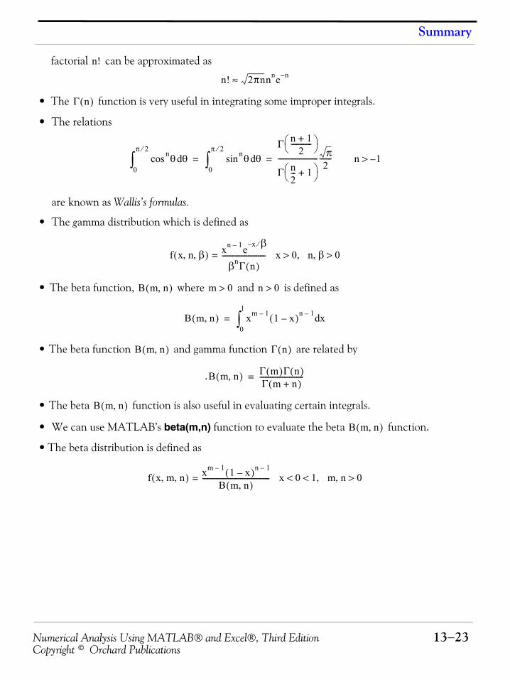
Numerical Analysis Using MATLAB® and Excel®, Third Edition 13−23Copyright © Orchard Publications
Summary
factorial can be approximated as
• The function is very useful in integrating some improper integrals.
• The relations
are known as Wallis’s formulas.
• The gamma distribution which is defined as
• The beta function, where and is defined as
• The beta function and gamma function are related by
.
• The beta function is also useful in evaluating certain integrals.
• We can use MATLAB’s beta(m,n) function to evaluate the beta function.
• The beta distribution is defined as
n!
n! 2πnnne n–≈
Γ n( )
θncos θd0
π 2⁄
∫ θnsin θd0
π 2⁄
∫Γ n 1+
2------------⎝ ⎠
⎛ ⎞
Γ n2--- 1+⎝ ⎠
⎛ ⎞----------------------- π
2------- n 1–>= =
f x n β, ,( ) xn 1– e x β⁄–
βnΓ n( )-------------------------= x 0 n β 0>,,>
B m n,( ) m 0> n 0>
B m n,( ) xm 1– 1 x–( )n 1– xd0
1
∫=
B m n,( ) Γ n( )
B m n,( ) Γ m( )Γ n( )Γ m n+( )-------------------------=
B m n,( )
B m n,( )
f x m n, ,( ) xm 1– 1 x–( )n 1–
B m n,( )---------------------------------------= x 0 1< m n 0>,,<
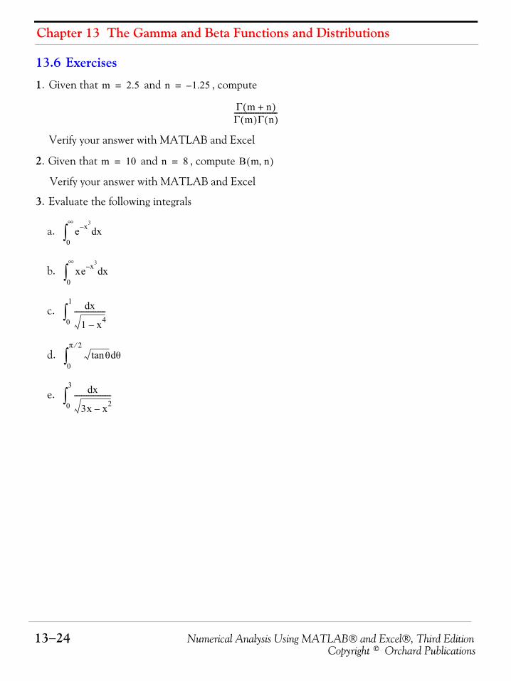
Chapter 13 The Gamma and Beta Functions and Distributions
13−24 Numerical Analysis Using MATLAB® and Excel®, Third EditionCopyright © Orchard Publications
13.6 Exercises
1. Given that and , compute
Verify your answer with MATLAB and Excel
2. Given that and , compute
Verify your answer with MATLAB and Excel
3. Evaluate the following integrals
a.
b.
c.
d.
e.
m 2.5= n 1.25–=
Γ m n+( )Γ m( )Γ n( )-------------------------
m 10= n 8= B m n,( )
e x3– xd0
∞
∫
xe x3– xd0
∞
∫
xd
1 x4–------------------
0
1
∫
θtan θd0
π 2⁄
∫
xd
3x x2–---------------------
0
3
∫
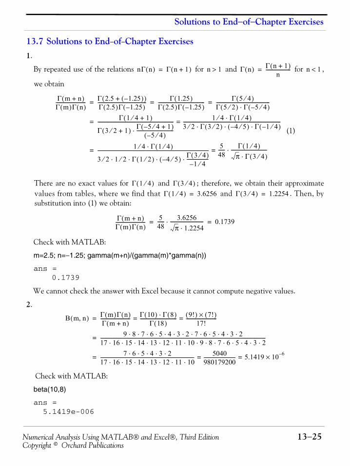
Numerical Analysis Using MATLAB® and Excel®, Third Edition 13−25Copyright © Orchard Publications
Solutions to End−of−Chapter Exercises
13.7 Solutions to End−of−Chapter Exercises1.
By repeated use of the relations for and for ,
we obtain
(1)
There are no exact values for and ; therefore, we obtain their approximatevalues from tables, where we find that and . Then, bysubstitution into (1) we obtain:
Check with MATLAB:
m=2.5; n=−1.25; gamma(m+n)/(gamma(m)*gamma(n))
ans = 0.1739
We cannot check the answer with Excel because it cannot compute negative values.
2.
Check with MATLAB:
beta(10,8)
ans = 5.1419e-006
nΓ n( ) Γ n 1+( )= n 1> Γ n( ) Γ n 1+( )n
---------------------= n 1<
Γ m n+( )Γ m( )Γ n( )------------------------- Γ 2.5 1.25–( )+( )
Γ 2.5( )Γ 1.25–( )----------------------------------------- Γ 1.25( )
Γ 2.5( )Γ 1.25–( )--------------------------------------- Γ 5 4⁄( )
Γ 5 2⁄( ) Γ 5– 4⁄( )⋅---------------------------------------------= = =
Γ 1 4⁄ 1+( )
Γ 3 2⁄ 1+( ) Γ 5– 4⁄ 1+( )5– 4⁄( )
-------------------------------⋅---------------------------------------------------------------- 1 4⁄ Γ 1 4⁄( )⋅
3 2⁄ Γ 3 2⁄( ) 4– 5⁄( ) Γ 1– 4⁄( )⋅ ⋅ ⋅----------------------------------------------------------------------------------==
1 4⁄ Γ 1 4⁄( )⋅
3 2⁄ 1 2⁄ Γ 1 2⁄( ) 4– 5⁄( )⋅ ⋅ ⋅ Γ 3 4⁄( )1– 4⁄
------------------⋅---------------------------------------------------------------------------------------------- 5
48------ Γ 1 4⁄( )
π Γ 3 4⁄( )⋅------------------------------⋅==
Γ 1 4⁄( ) Γ 3 4⁄( )Γ 1 4⁄( ) 3.6256= Γ 3 4⁄( ) 1.2254=
Γ m n+( )Γ m( )Γ n( )------------------------- 5
48------ 3.6256
π 1.2254⋅----------------------------⋅ 0.1739= =
B m n,( ) Γ m( )Γ n( )Γ m n+( )------------------------- Γ 10( ) Γ 8( )⋅
Γ 18( )------------------------------- 9!( ) 7!( )×
17!--------------------------= ==
9 8 7 6 5 4 3 2 7 6 5 4 3 2⋅ ⋅ ⋅ ⋅ ⋅ ⋅ ⋅ ⋅ ⋅ ⋅ ⋅ ⋅ ⋅17 16 15 14 13 12 11 10 9 8 7 6 5 4 3 2⋅ ⋅ ⋅ ⋅ ⋅ ⋅ ⋅ ⋅ ⋅ ⋅ ⋅ ⋅ ⋅ ⋅ ⋅-------------------------------------------------------------------------------------------------------------------------------------------=
7 6 5 4 3 2⋅ ⋅ ⋅ ⋅ ⋅17 16 15 14 13 12 11 10⋅ ⋅ ⋅ ⋅ ⋅ ⋅ ⋅------------------------------------------------------------------------------- 5040
980179200--------------------------- 5.1419 10 6–×= ==
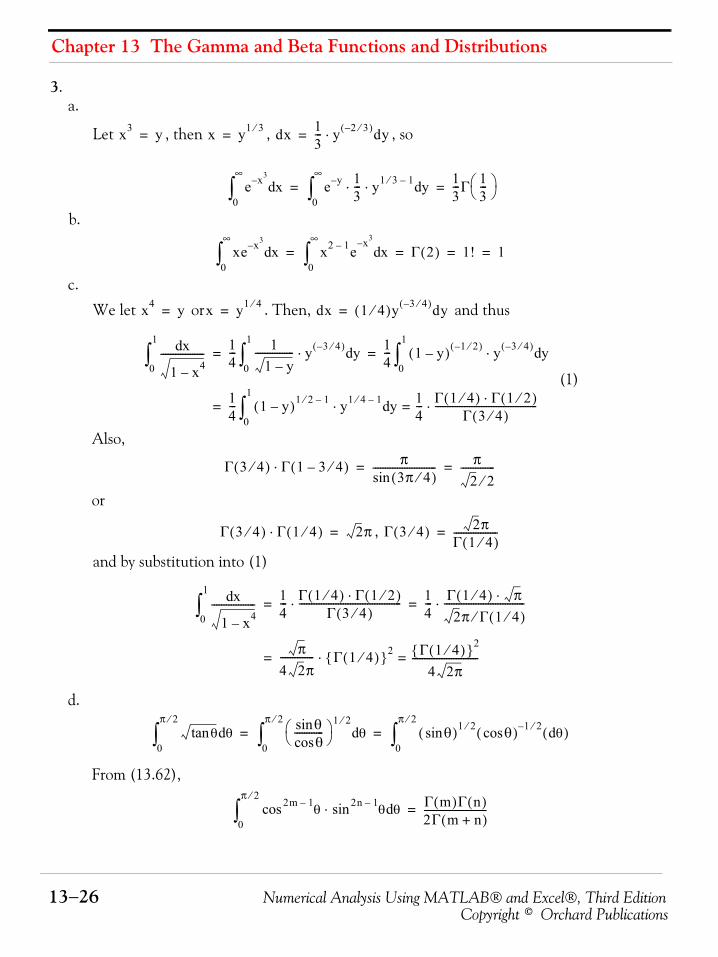
Chapter 13 The Gamma and Beta Functions and Distributions
13−26 Numerical Analysis Using MATLAB® and Excel®, Third EditionCopyright © Orchard Publications
3.a.
Let , then , , so
b.
c.
We let or . Then, and thus
(1)
Also,
or
,
and by substitution into (1)
d.
From (13.62),
x3 y= x y1 3⁄= dx 13--- y 2– 3⁄( )dy⋅=
e x3– xd0
∞
∫ e y– 13--- y1 3⁄ 1– yd⋅ ⋅
0
∞
∫13---Γ 1
3---⎝ ⎠
⎛ ⎞= =
xe x3– xd0
∞
∫ x2 1– ex3–
xd0
∞
∫ Γ 2( ) 1! 1= = = =
x4 y= x y1 4⁄= dx 1 4⁄( )y 3– 4⁄( )dy=
xd
1 x4–------------------
0
1
∫14--- 1
1 y–---------------- y 3– 4⁄( )⋅ yd
0
1
∫14--- 1 y–( ) 1– 2⁄( ) y 3– 4⁄( )⋅ yd
0
1
∫= =
14--- 1 y–( )1 2⁄ 1– y1 4⁄ 1–⋅ yd
0
1
∫14--- Γ 1 4⁄( ) Γ 1 2⁄( )⋅
Γ 3 4⁄( )------------------------------------------⋅==
Γ 3 4⁄( ) Γ 1 3 4⁄–( )⋅ π3π 4⁄( )sin
-------------------------- π2 2⁄
--------------= =
Γ 3 4⁄( ) Γ 1 4⁄( )⋅ 2π= Γ 3 4⁄( ) 2πΓ 1 4⁄( )------------------=
xd
1 x4–------------------
0
1
∫14--- Γ 1 4⁄( ) Γ 1 2⁄( )⋅
Γ 3 4⁄( )------------------------------------------⋅ 1
4--- Γ 1 4⁄( ) π⋅
2π Γ 1 4⁄( )⁄---------------------------------⋅= =
π4 2π-------------- Γ 1 4⁄( ){ }2⋅ Γ 1 4⁄( ){ }2
4 2π---------------------------==
θtan θd0
π 2⁄
∫θsinθcos
------------⎝ ⎠⎛ ⎞ 1 2⁄
θd0
π 2⁄
∫ θsin( )1 2⁄ θcos( ) 1– 2⁄ θd( )0
π 2⁄
∫= =
θ2m 1–cos θ2n 1–sin⋅ θd0
π 2⁄
∫ Γ m( )Γ n( )2Γ m n+( )--------------------------=
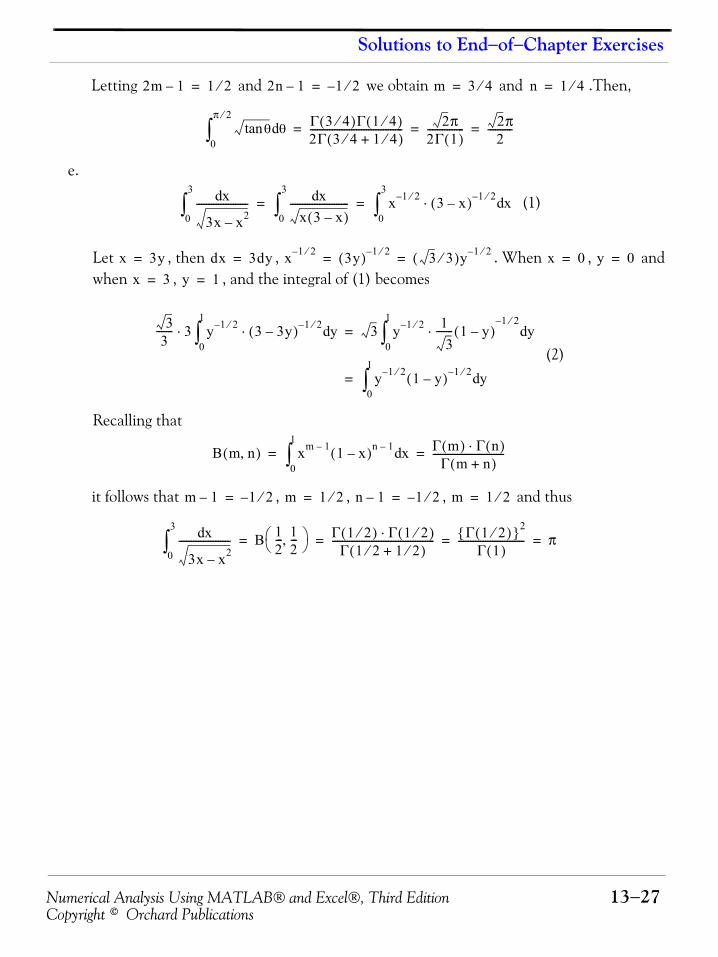
Numerical Analysis Using MATLAB® and Excel®, Third Edition 13−27Copyright © Orchard Publications
Solutions to End−of−Chapter Exercises
Letting and we obtain and .Then,
e.
(1)
Let , then , . When , andwhen , , and the integral of (1) becomes
(2)
Recalling that
it follows that , , , and thus
2m 1– 1 2⁄= 2n 1– 1– 2⁄= m 3 4⁄= n 1 4⁄=
θtan θd0
π 2⁄
∫ Γ 3 4⁄( )Γ 1 4⁄( )2Γ 3 4⁄ 1 4⁄+( )-------------------------------------- 2π
2Γ 1( )--------------- 2π
2----------= = =
xd
3x x2–---------------------
0
3
∫ xdx 3 x–( )
------------------------0
3
∫ x 1– 2⁄ 3 x–( ) 1– 2⁄⋅ xd0
3
∫= =
x 3y= dx 3dy= x 1– 2⁄ 3y( ) 1– 2⁄ 3 3⁄( )y 1– 2⁄= = x 0= y 0=
x 3= y 1=
33
------- 3 y 1– 2⁄ 3 3y–( ) 1– 2⁄⋅ yd0
1
∫⋅ 3 y 1– 2⁄ 13
------- 1 y–( )1– 2⁄
⋅ yd0
1
∫=
y 1– 2⁄ 1 y–( ) 1– 2⁄ yd0
1
∫=
B m n,( ) xm 1– 1 x–( )n 1– xd0
1
∫ Γ m( ) Γ n( )⋅Γ m n+( )
-----------------------------= =
m 1– 1– 2⁄= m 1 2⁄= n 1– 1– 2⁄= m 1 2⁄=
xd
3x x2–---------------------
0
3
∫ B 12--- 1
2---,⎝ ⎠
⎛ ⎞ Γ 1 2⁄( ) Γ 1 2⁄( )⋅Γ 1 2⁄ 1 2⁄+( )
------------------------------------------ Γ 1 2⁄( ){ }2
Γ 1( )--------------------------- π= = = =
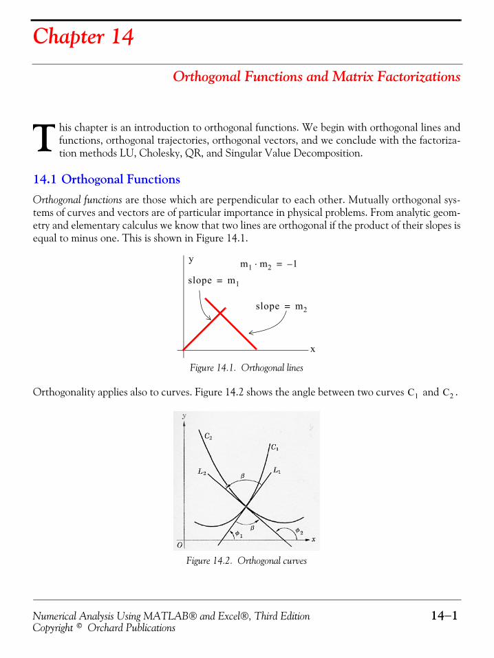
Numerical Analysis Using MATLAB® and Excel®, Third Edition 14−1Copyright © Orchard Publications
Chapter 14
Orthogonal Functions and Matrix Factorizations
his chapter is an introduction to orthogonal functions. We begin with orthogonal lines andfunctions, orthogonal trajectories, orthogonal vectors, and we conclude with the factoriza-tion methods LU, Cholesky, QR, and Singular Value Decomposition.
14.1 Orthogonal FunctionsOrthogonal functions are those which are perpendicular to each other. Mutually orthogonal sys-tems of curves and vectors are of particular importance in physical problems. From analytic geom-etry and elementary calculus we know that two lines are orthogonal if the product of their slopes isequal to minus one. This is shown in Figure 14.1.
Figure 14.1. Orthogonal lines
Orthogonality applies also to curves. Figure 14.2 shows the angle between two curves and .
Figure 14.2. Orthogonal curves
T
slope m1=
slope m2=
x
y m1 m2⋅ 1–=
C1 C2
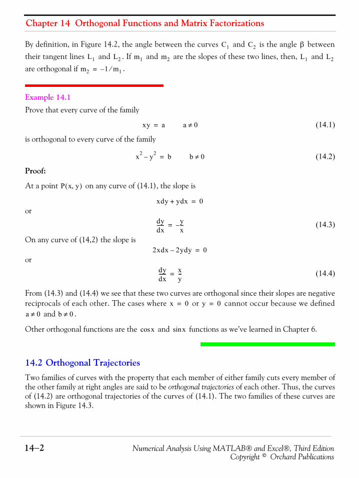
Chapter 14 Orthogonal Functions and Matrix Factorizations
14−2 Numerical Analysis Using MATLAB® and Excel®, Third EditionCopyright © Orchard Publications
By definition, in Figure 14.2, the angle between the curves and is the angle betweentheir tangent lines and . If and are the slopes of these two lines, then, and are orthogonal if .
Example 14.1 Prove that every curve of the family
(14.1)
is orthogonal to every curve of the family
(14.2)
Proof:
At a point on any curve of (14.1), the slope is
or
(14.3)
On any curve of (14,2) the slope is
or
(14.4)
From (14.3) and (14.4) we see that these two curves are orthogonal since their slopes are negativereciprocals of each other. The cases where or cannot occur because we defined
and .
Other orthogonal functions are the and functions as we’ve learned in Chapter 6.
14.2 Orthogonal TrajectoriesTwo families of curves with the property that each member of either family cuts every member ofthe other family at right angles are said to be orthogonal trajectories of each other. Thus, the curvesof (14.2) are orthogonal trajectories of the curves of (14.1). The two families of these curves areshown in Figure 14.3.
C1 C2 β
L1 L2 m1 m2 L1 L2
m2 1– m1⁄=
xy a= a 0≠
x2 y2– b= b 0≠
P x y,( )
xdy ydx+ 0=
dydx------ y
x---–=
2xdx 2ydy– 0=
dydx------ x
y---=
x 0= y 0=
a 0≠ b 0≠
xcos xsin
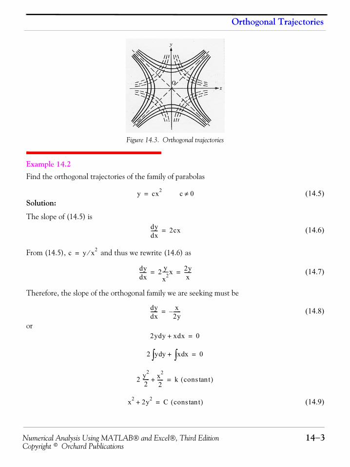
Numerical Analysis Using MATLAB® and Excel®, Third Edition 14−3Copyright © Orchard Publications
Orthogonal Trajectories
Figure 14.3. Orthogonal trajectories
Example 14.2 Find the orthogonal trajectories of the family of parabolas
(14.5)Solution:
The slope of (14.5) is
(14.6)
From (14.5), and thus we rewrite (14.6) as
(14.7)
Therefore, the slope of the orthogonal family we are seeking must be
(14.8)
or
(14.9)
y cx2= c 0≠
dydx------ 2cx=
c y x2⁄=
dydx------ 2 y
x2-----x 2y
x------= =
dydx------ x
2y------–=
2ydy xdx+ 0=
2 y y x xd∫+d∫ 0=
2 y2
2----- x2
2-----+ k cons ttan( )=
x2 2y2+ C cons ttan( )=
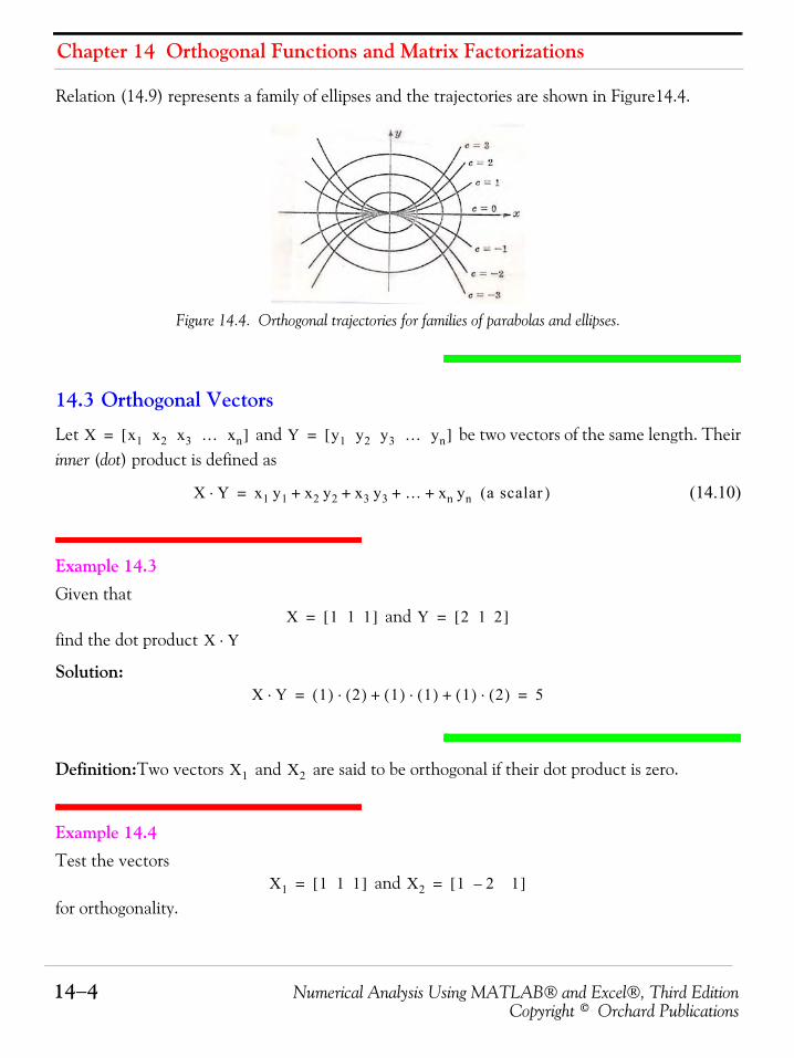
Chapter 14 Orthogonal Functions and Matrix Factorizations
14−4 Numerical Analysis Using MATLAB® and Excel®, Third EditionCopyright © Orchard Publications
Relation (14.9) represents a family of ellipses and the trajectories are shown in Figure14.4.
Figure 14.4. Orthogonal trajectories for families of parabolas and ellipses.
14.3 Orthogonal Vectors
Let and be two vectors of the same length. Theirinner (dot) product is defined as
(14.10)
Example 14.3 Given that
and find the dot product
Solution:
Definition:Two vectors and are said to be orthogonal if their dot product is zero.
Example 14.4 Test the vectors
and for orthogonality.
X x1 x2 x3 … xn[ ]= Y y1 y2 y3 … yn[ ]=
X Y⋅ x1 y1 x2 y2 x3 y3 … xn yn (a scalar )+ + + +=
X 1 1 1[ ]= Y 2 1 2[ ]=
X Y⋅
X Y⋅ 1( ) 2( )⋅ 1( ) 1( )⋅ 1( ) 2( )⋅+ + 5= =
X1 X2
X1 1 1 1[ ]= X2 1 2– 1[ ]=
Numerical Analysis Using MATLAB® and Excel®, Third Edition 14−5Copyright © Orchard Publications
Orthogonal Vectors
Solution:
Therefore, the vectors and are orthogonal to each other.
With any vector we may associate a unique unit vector which is obtained by dividingeach component of by each magnitude defined as
where represents an element of the vector . This process is called normalization.
Example 14.5 Given that
compute the unit vector .
Solution:
First, we compute the magnitude . For this example,
To compute the unit vector we divide each element of by the magnitude . Thus,
A basis that consists of mutually orthogonal vectors is referred to as an orthogonal basis. If thesevectors are also unit vectors, the basis is called orthonormal basis.
If the column (or row) vectors of a square matrix are mutually orthogonal unit vectors, thematrix is orthogonal and
(14.11)
where is the transpose of and is the identity matrix.
X1 X2⋅ 1( ) 1( )⋅ 1( ) 2–( )⋅ 1( ) 1( )⋅+ + 0= =
X1 X2
X 0≠ UX X
X x12 x2
2 … xn2+ + +=
xi X
X 2 4 4[ ]=
UX
X
X 22 42 42+ + 6= =
UX X X
UX26--- 46
--- 46--- 1
2--- 23
--- 23---= =
AA
A AT⋅ I=
AT A I
Chapter 14 Orthogonal Functions and Matrix Factorizations
14−6 Numerical Analysis Using MATLAB® and Excel®, Third EditionCopyright © Orchard Publications
Example 14.6 Given that
find an orthonormal set of eigenvectors* and verify that the result satisfies (14.11).
Solution:
First, we find the eigenvalues of the matrix from the relation where for thisexample
from which and and as we’ve learned in Chapter 5, with these eigenvalueswe can obtain an infinite number of eigenvectors. To find a square matrix such that
we begin with
(14.12)
or
(14.13)
Equating like terms we obtain
From the second equation we obtain and by substitution into the first we obtain or
* It is strongly suggested that the reader reviews the definitions of eigenvalues and eigenvectors in Chapter 5 at this time.
A 1 2⁄ 1 4⁄1 2⁄ 1 2⁄
=
A det A λI–( ) 0=
det 1 2⁄ 1 4⁄1 2⁄ 1 2⁄
λ 1 00 1
–⎝ ⎠⎜ ⎟⎛ ⎞
0=
det 1 2 λ–⁄ 1 4⁄1 2⁄ 1 2 λ–⁄
0=
λ2 λ– 3 16⁄+ 0=
λ1 1 4⁄= λ2 3 4⁄=
2 2× Z
Z ZT⋅ I=
z1 z2
z1– z2
z1 z1–
z2 z2
⋅ 1 00 1
=
z12 z2
2+ z– 12 z2
2+
z– 12 z2
2+ z12 z2
2+
1 00 1
=
z12 z2
2+ 1= z– 12 z2
2+ 0=
z12 z2
2= 2z12 1=
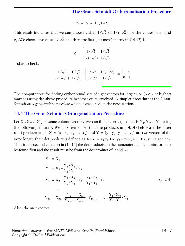
Numerical Analysis Using MATLAB® and Excel®, Third Edition 14−7Copyright © Orchard Publications
The Gram-Schmidt Orthogonalization Procedure
This result indicates that we can choose either or for the values of and
.We choose the value and then the first (left most) matrix in (14.12) is
and as a check,
The computations for finding orthonormal sets of eigenvectors for larger size ( or higher)matrices using the above procedure becomes quite involved. A simpler procedure is the Gram-Schmidt orthogonalization procedure which is discussed on the next section.
14.4 The Gram-Schmidt Orthogonalization Procedure
Let be some column vectors. We can find an orthogonal basis usingthe following relations. We must remember that the products in (14.14) below are the inner(dot) products and if and are two vectors of thesame length their dot product is defined as .Thus in the second equation in (14.14) the dot products on the numerator and denominator mustbe found first and the result must be from the dot product of it and
(14.14)
Also, the unit vectors
z1 z2 1 2±( )⁄= =
1 2⁄ 1 2–( )⁄ z1
z2 1 2⁄
Z 1 2⁄ 1 2⁄
1 2–( )⁄ 1 2⁄=
1 2⁄ 1 2⁄
1 2–( )⁄ 1 2⁄
1 2⁄ 1 2–( )⁄
1 2⁄ 1 2⁄⋅ 1 0
0 1=
3 3×
X1 X2 …Xm, , Y1 Y2 …Ym, ,
X x1 x2 x3 … xn[ ]= Y y1 y2 y3 … yn[ ]=
X Y⋅ x1 y1 x2 y2 x3 y3 … xn yn (a scalar )+ + + +=
Y1
Y1 X1=
Y2 X2Y1 X2⋅Y1 Y1⋅------------------ Y1⋅–=
Y3 X3Y2 X3⋅Y2 Y2⋅------------------ Y2⋅–
Y1 X3⋅Y1 Y1⋅------------------ Y1⋅–=
…
Ym XmYm 1– Xm⋅
Ym 1– Ym 1–⋅--------------------------------- Ym 1–⋅ …––
Y1 Xm⋅Y1 Y1⋅------------------- Y1⋅–=
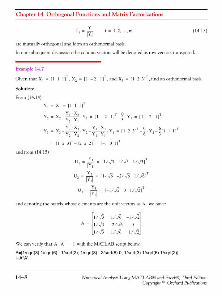
Chapter 14 Orthogonal Functions and Matrix Factorizations
14−8 Numerical Analysis Using MATLAB® and Excel®, Third EditionCopyright © Orchard Publications
(14.15)
are mutually orthogonal and form an orthonormal basis.
In our subsequent discussion the column vectors will be denoted as row vectors transposed.
Example 14.7
Given that , , and , find an orthonormal basis.
Solution:
From (14.14)
and from (14.15)
and denoting the matrix whose elements are the unit vectors as , we have:
We can verify that with the MATLAB script below.
A=[1/sqrt(3) 1/sqrt(6) −1/sqrt(2); 1/sqrt(3) −2/sqrt(6) 0; 1/sqrt(3) 1/sqrt(6) 1/sqrt(2)];I=A*A'
UiYiYi--------= i 1 2 … m, , ,=
X1 1 1 1[ ]T= X2 1 2 1–[ ]T= X3 1 2 3[ ]T=
Y1 X1 1 1 1[ ]T= =
Y2 X2Y1 X2⋅Y1 Y1⋅------------------ Y1⋅– 1 2 1–[ ]T 0
3--- Y1⋅– 1 2 1–[ ]T= = =
Y3 X3Y2 X3⋅Y2 Y2⋅------------------ Y2⋅–
Y1 X3⋅Y1 Y1⋅------------------ Y1⋅– 1 2 3[ ]T 0
6--- Y2⋅–
63--- 1 1 1[ ]T–= =
1 2 3[ ]T 2 2 2[ ]T– 1– 0 1[ ]T==
U1Y1Y1--------- 1 3⁄ 1 3 1 3⁄⁄[ ]
T= =
U2Y2Y2--------- 1 6⁄ 2– 6 1 6⁄⁄[ ]
T= =
U3Y3Y3--------- 1– 2⁄ 0 1 2⁄[ ]
T= =
A
A1 3⁄ 1 6⁄ 1– 2⁄
1 3⁄ 2– 6⁄ 0
1 3⁄ 1 6⁄ 1 2⁄
=
A AT⋅ I=
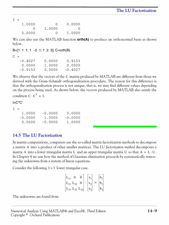
Numerical Analysis Using MATLAB® and Excel®, Third Edition 14−9Copyright © Orchard Publications
The LU Factorization
I = 1.0000 0 0.0000 0 1.0000 0 0.0000 0 1.0000
We can also use the MATLAB function orth(A) to produce an orthonormal basis as shownbelow.
B=[1 1 1; 1 −2 1; 1 2 3]; C=orth(B)
C = -0.4027 0.0000 0.9153 0.0000 1.0000 0.0000 -0.9153 0.0000 -0.4027
We observe that the vectors of the matrix produced by MATLAB are different from those wederived with the Gram-Schmidt orthogonalization procedure. The reason for this difference isthat the orthogonalization process is not unique, that is, we may find different values dependingon the process being used. As shown below, the vectors produced by MATLAB also satisfy the
condition .
I=C*C'
I = 1.0000 -0.0000 0.0000 -0.0000 1.0000 -0.0000 0.0000 -0.0000 1.0000
14.5 The LU FactorizationIn matrix computations, computers use the so-called matrix factorization methods to decomposea matrix into a product of other smaller matrices. The LU factorization method decomposes amatrix into a lower triangular matrix and an upper triangular matrix so that .In Chapter 4 we saw how the method of Gaussian elimination proceeds by systematically remov-ing the unknowns from a system of linear equations.
Consider the following lower triangular case.
The unknowns are found from
C
C CT⋅ I=
AA L U A L U⋅=
3 3×
L11 0 0L21 L22 0L31 L32 L33
x1
x2
x3
⋅b1
b2
b3
=
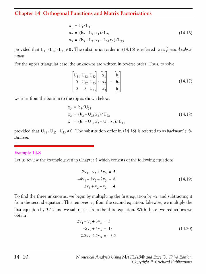
Chapter 14 Orthogonal Functions and Matrix Factorizations
14−10 Numerical Analysis Using MATLAB® and Excel®, Third EditionCopyright © Orchard Publications
(14.16)
provided that . The substitution order in (14.16) is referred to as forward substi-tution.
For the upper triangular case, the unknowns are written in reverse order. Thus, to solve
(14.17)
we start from the bottom to the top as shown below.
(14.18)
provided that . The substitution order in (14.18) is referred to as backward sub-stitution.
Example 14.8 Let us review the example given in Chapter 4 which consists of the following equations.
(14.19)
To find the three unknowns, we begin by multiplying the first equation by and subtracting itfrom the second equation. This removes from the second equation. Likewise, we multiply the
first equation by and we subtract it from the third equation. With these two reductions weobtain
(14.20)
x1 b1 L11⁄=
x2 b2 L21 x1–( ) L22⁄=
x3 b3 L31 x1 L31 x2––( ) L33⁄=
L11 L22 L33⋅ ⋅ 0≠
U11 U12 U13
0 U22 U23
0 0 U33
x1
x2
x3
⋅b1
b2
b3
=
x3 b3 U33⁄=
x2 b2 U23 x3–( ) U22⁄=
x1 b1 U12 x2 U13 x3––( ) U11⁄=
U11 U22 U33⋅ ⋅ 0≠
2v1 v2– 3v3+ 5=
4v1 3v2 2v3––– 8=
3v1 v2 v3–+ 4=
2–
v1
3 2⁄
2v1 v2– 3v3+ 5=
5v2 4v3+– 18=
2.5v2 5.5– v3 3.5–=
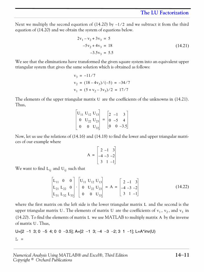
Numerical Analysis Using MATLAB® and Excel®, Third Edition 14−11Copyright © Orchard Publications
The LU Factorization
Next we multiply the second equation of (14.20) by and we subtract it from the thirdequation of (14.20) and we obtain the system of equations below.
(14.21)
We see that the eliminations have transformed the given square system into an equivalent uppertriangular system that gives the same solution which is obtained as follows:
The elements of the upper triangular matrix are the coefficients of the unknowns in (14.21).Thus,
Now, let us use the relations of (14.16) and (14.18) to find the lower and upper triangular matri-ces of our example where
We want to find and such that
(14.22)
where the first matrix on the left side is the lower triangular matrix and the second is theupper triangular matrix . The elements of matrix are the coefficients of , , and in(14.20). To find the elements of matrix we use MATLAB to multiply matrix by the inverseof matrix . Thus,
U=[2 −1 3; 0 −5 4; 0 0 −3.5]; A=[2 −1 3; −4 −3 −2; 3 1 −1]; L=A*inv(U)
L =
1 2⁄–
2v1 v2– 3v3+ 5=
5v2 4v3+– 18=
3.5– v3 5.5=
v3 11– 7⁄=
v2 18 4v3–( ) 5–( )⁄ 34 7⁄–= =
v1 5 v2 3v3–+( ) 2⁄ 17 7⁄= =
U
U11 U12 U13
0 U22 U23
0 0 U33
2 1– 30 5– 40 0 3.5–
=
A2 1– 34– 3– 2–3 1 1–
=
Lij Uij
L11 0 0L21 L22 0L31 L32 L33
U11 U12 U13
0 U22 U23
0 0 U33
⋅ A2 1– 34– 3– 2–3 1 1–
= =
LU U v1 v2 v3
L AU
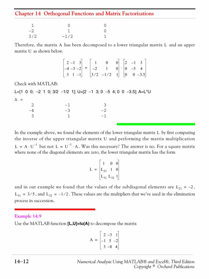
Chapter 14 Orthogonal Functions and Matrix Factorizations
14−12 Numerical Analysis Using MATLAB® and Excel®, Third EditionCopyright © Orchard Publications
1 0 0 -2 1 0 3/2 -1/2 1
Therefore, the matrix has been decomposed to a lower triangular matrix and an uppermatrix as shown below.
Check with MATLAB:
L=[1 0 0; −2 1 0; 3/2 −1/2 1]; U=[2 −1 3; 0 −5 4; 0 0 −3.5]; A=L*U
A = 2 -1 3 -4 -3 -2 3 1 -1
In the example above, we found the elements of the lower triangular matrix by first computingthe inverse of the upper triangular matrix and performing the matrix multiplication
but not . Was this necessary? The answer is no. For a square matrixwhere none of the diagonal elements are zero, the lower triangular matrix has the form
and in our example we found that the values of the subdiagonal elements are ,, and . These values are the multipliers that we’ve used in the elimination
process in succession.
Example 14.9 Use the MATLAB function [L,U]=lu(A) to decompose the matrix
A LU
2 1– 34– 3– 2–3 1 1–
1 0 02– 1 0
3 2⁄ 1 2⁄– 1
2 1– 30 5– 40 0 3.5–
⋅=
LU
L A U 1–⋅= L U 1– A⋅=
L1 0 0
L21 1 0L31 L32 1
=
L21 2–=
L31 3 5⁄= L32 1– 2⁄=
A2 3– 11– 5 2–3 8– 4
=
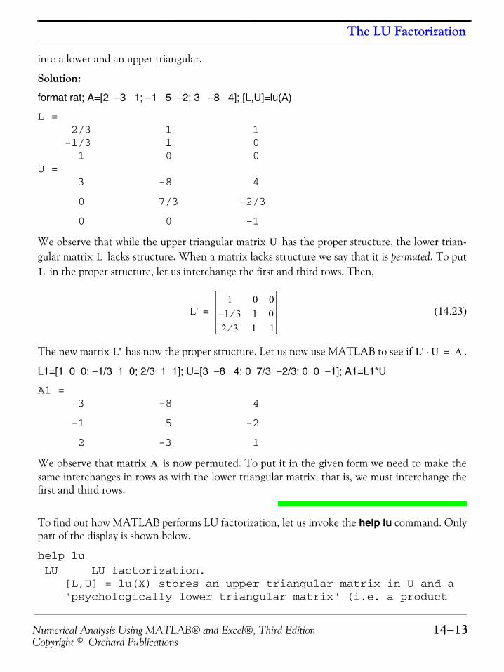
Numerical Analysis Using MATLAB® and Excel®, Third Edition 14−13Copyright © Orchard Publications
The LU Factorization
into a lower and an upper triangular.
Solution:
format rat; A=[2 −3 1; −1 5 −2; 3 −8 4]; [L,U]=lu(A)
L = 2/3 1 1 -1/3 1 0 1 0 0 U = 3 -8 4
0 7/3 -2/3
0 0 -1
We observe that while the upper triangular matrix has the proper structure, the lower trian-gular matrix lacks structure. When a matrix lacks structure we say that it is permuted. To put
in the proper structure, let us interchange the first and third rows. Then,
(14.23)
The new matrix has now the proper structure. Let us now use MATLAB to see if .
L1=[1 0 0; −1/3 1 0; 2/3 1 1]; U=[3 −8 4; 0 7/3 −2/3; 0 0 −1]; A1=L1*U
A1 = 3 -8 4
-1 5 -2
2 -3 1
We observe that matrix is now permuted. To put it in the given form we need to make thesame interchanges in rows as with the lower triangular matrix, that is, we must interchange thefirst and third rows.
To find out how MATLAB performs LU factorization, let us invoke the help lu command. Onlypart of the display is shown below.
help lu
LU LU factorization. [L,U] = lu(X) stores an upper triangular matrix in U and a "psychologically lower triangular matrix" (i.e. a product
UL
L
L'1 0 0
1 3⁄– 1 02 3⁄ 1 1
=
L' L' U⋅ A=
A
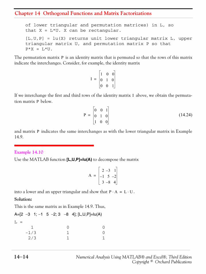
Chapter 14 Orthogonal Functions and Matrix Factorizations
14−14 Numerical Analysis Using MATLAB® and Excel®, Third EditionCopyright © Orchard Publications
of lower triangular and permutation matrices) in L, so that X = L*U. X can be rectangular. [L,U,P] = lu(X) returns unit lower triangular matrix L, upper triangular matrix U, and permutation matrix P so that P*X = L*U.
The permutation matrix is an identity matrix that is permuted so that the rows of this matrixindicate the interchanges. Consider, for example, the identity matrix
If we interchange the first and third rows of the identity matrix above, we obtain the permuta-tion matrix below.
(14.24)
and matrix indicates the same interchanges as with the lower triangular matrix in Example14.9.
Example 14.10 Use the MATLAB function [L,U,P]=lu(A) to decompose the matrix
into a lower and an upper triangular and show that .
Solution:This is the same matrix as in Example 14.9. Thus,
A=[2 −3 1; −1 5 −2; 3 −8 4]; [L,U,P]=lu(A)
L = 1 0 0 -1/3 1 0 2/3 1 1
P
I1 0 00 1 00 0 1
=
IP
P0 0 10 1 01 0 0
=
P
A2 3– 11– 5 2–3 8– 4
=
P A⋅ L U⋅=
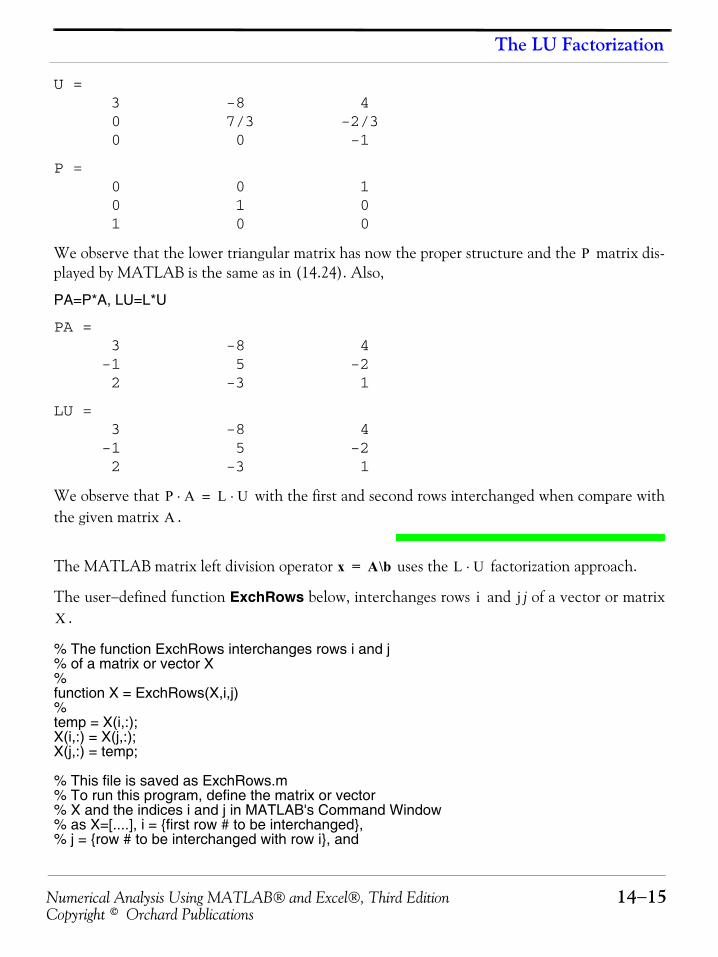
Numerical Analysis Using MATLAB® and Excel®, Third Edition 14−15Copyright © Orchard Publications
The LU Factorization
U = 3 -8 4 0 7/3 -2/3 0 0 -1
P = 0 0 1 0 1 0 1 0 0
We observe that the lower triangular matrix has now the proper structure and the matrix dis-played by MATLAB is the same as in (14.24). Also,
PA=P*A, LU=L*U
PA = 3 -8 4 -1 5 -2 2 -3 1
LU = 3 -8 4 -1 5 -2 2 -3 1
We observe that with the first and second rows interchanged when compare withthe given matrix .
The MATLAB matrix left division operator uses the factorization approach.
The user−defined function ExchRows below, interchanges rows and j of a vector or matrix.
% The function ExchRows interchanges rows i and j % of a matrix or vector X%function X = ExchRows(X,i,j)%temp = X(i,:);X(i,:) = X(j,:);X(j,:) = temp; % This file is saved as ExchRows.m% To run this program, define the matrix or vector% X and the indices i and j in MATLAB's Command Window% as X=[....], i = {first row # to be interchanged},% j = {row # to be interchanged with row i}, and
P
P A⋅ L U⋅=
A
x A\b= L U⋅
i jX
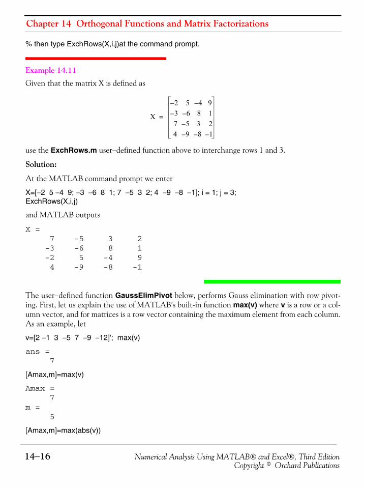
Chapter 14 Orthogonal Functions and Matrix Factorizations
14−16 Numerical Analysis Using MATLAB® and Excel®, Third EditionCopyright © Orchard Publications
% then type ExchRows(X,i,j)at the command prompt.
Example 14.11 Given that the matrix X is defined as
use the ExchRows.m user−defined function above to interchange rows 1 and 3.
Solution:
At the MATLAB command prompt we enter
X=[−2 5 −4 9; −3 −6 8 1; 7 −5 3 2; 4 −9 −8 −1]; i = 1; j = 3;ExchRows(X,i,j)
and MATLAB outputs
X = 7 -5 3 2 -3 -6 8 1 -2 5 -4 9 4 -9 -8 -1
The user−defined function GaussElimPivot below, performs Gauss elimination with row pivot-ing. First, let us explain the use of MATLAB’s built-in function max(v) where v is a row or a col-umn vector, and for matrices is a row vector containing the maximum element from each column.As an example, let
v=[2 −1 3 −5 7 −9 −12]'; max(v)
ans = 7
[Amax,m]=max(v)
Amax = 7m = 5
[Amax,m]=max(abs(v))
X
2– 5 4– 93– 6– 8 17 5– 3 24 9– 8– 1–
=
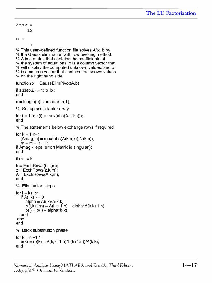
Numerical Analysis Using MATLAB® and Excel®, Third Edition 14−17Copyright © Orchard Publications
The LU Factorization
Amax = 12
m = 7% This user−defined function file solves A*x=b by% the Gauss elimination with row pivoting method.% A is a matrix that contains the coefficients of % the system of equations, x is a column vector that% will display the computed unknown values, and b % is a column vector that contains the known values% on the right hand side.
function x = GaussElimPivot(A,b) if size(b,2) > 1; b=b'; end
n = length(b); z = zeros(n,1);
% Set up scale factor array
for i = 1:n; z(i) = max(abs(A(i,1:n))); end
% The statements below exchange rows if required
for k = 1:n−1 [Amag,m] = max(abs(A(k:n,k))./z(k:n)); m = m + k − 1;if Amag < eps; error('Matrix is singular');end
if m ~= k
b = ExchRows(b,k,m);z = ExchRows(z,k,m);A = ExchRows(A,k,m); end
% Elimination steps
for i = k+1:n if A(i,k) ~= 0 alpha = A(i,k)/A(k,k); A(i,k+1:n) = A(i,k+1:n) − alpha*A(k,k+1:n) b(i) = b(i) − alpha*b(k); end endend
% Back substitution phase
for k = n:−1:1 b(k) = (b(k) − A(k,k+1:n)*b(k+1:n))/A(k,k);end
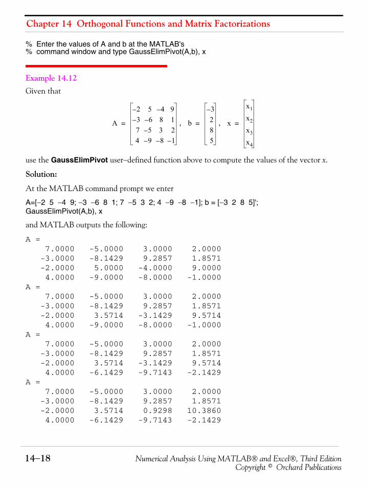
Chapter 14 Orthogonal Functions and Matrix Factorizations
14−18 Numerical Analysis Using MATLAB® and Excel®, Third EditionCopyright © Orchard Publications
% Enter the values of A and b at the MATLAB's % command window and type GaussElimPivot(A,b), x
Example 14.12 Given that
, ,
use the GaussElimPivot user−defined function above to compute the values of the vector x.
Solution:
At the MATLAB command prompt we enter
A=[−2 5 −4 9; −3 −6 8 1; 7 −5 3 2; 4 −9 −8 −1]; b = [−3 2 8 5]';GaussElimPivot(A,b), x
and MATLAB outputs the following:
A = 7.0000 -5.0000 3.0000 2.0000 -3.0000 -8.1429 9.2857 1.8571 -2.0000 5.0000 -4.0000 9.0000 4.0000 -9.0000 -8.0000 -1.0000A = 7.0000 -5.0000 3.0000 2.0000 -3.0000 -8.1429 9.2857 1.8571 -2.0000 3.5714 -3.1429 9.5714 4.0000 -9.0000 -8.0000 -1.0000A = 7.0000 -5.0000 3.0000 2.0000 -3.0000 -8.1429 9.2857 1.8571 -2.0000 3.5714 -3.1429 9.5714 4.0000 -6.1429 -9.7143 -2.1429A = 7.0000 -5.0000 3.0000 2.0000 -3.0000 -8.1429 9.2857 1.8571 -2.0000 3.5714 0.9298 10.3860 4.0000 -6.1429 -9.7143 -2.1429
A
2– 5 4– 93– 6– 8 17 5– 3 24 9– 8– 1–
= b
3–285
= x
x1
x2
x3
x4
=
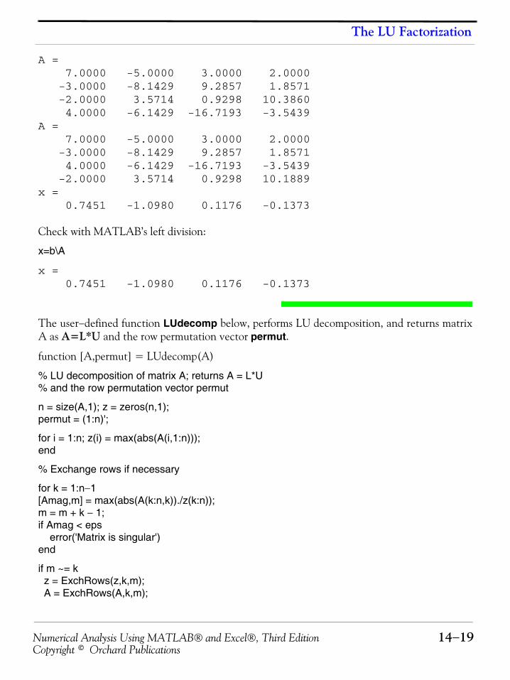
Numerical Analysis Using MATLAB® and Excel®, Third Edition 14−19Copyright © Orchard Publications
The LU Factorization
A = 7.0000 -5.0000 3.0000 2.0000 -3.0000 -8.1429 9.2857 1.8571 -2.0000 3.5714 0.9298 10.3860 4.0000 -6.1429 -16.7193 -3.5439A = 7.0000 -5.0000 3.0000 2.0000 -3.0000 -8.1429 9.2857 1.8571 4.0000 -6.1429 -16.7193 -3.5439 -2.0000 3.5714 0.9298 10.1889x = 0.7451 -1.0980 0.1176 -0.1373
Check with MATLAB’s left division:
x=b\A
x = 0.7451 -1.0980 0.1176 -0.1373
The user−defined function LUdecomp below, performs LU decomposition, and returns matrixA as A=L*U and the row permutation vector permut.
function [A,permut] = LUdecomp(A)
% LU decomposition of matrix A; returns A = L*U% and the row permutation vector permut
n = size(A,1); z = zeros(n,1);permut = (1:n)';
for i = 1:n; z(i) = max(abs(A(i,1:n))); end
% Exchange rows if necessary
for k = 1:n−1[Amag,m] = max(abs(A(k:n,k))./z(k:n));m = m + k − 1;if Amag < eps error('Matrix is singular')end
if m ~= k z = ExchRows(z,k,m); A = ExchRows(A,k,m);
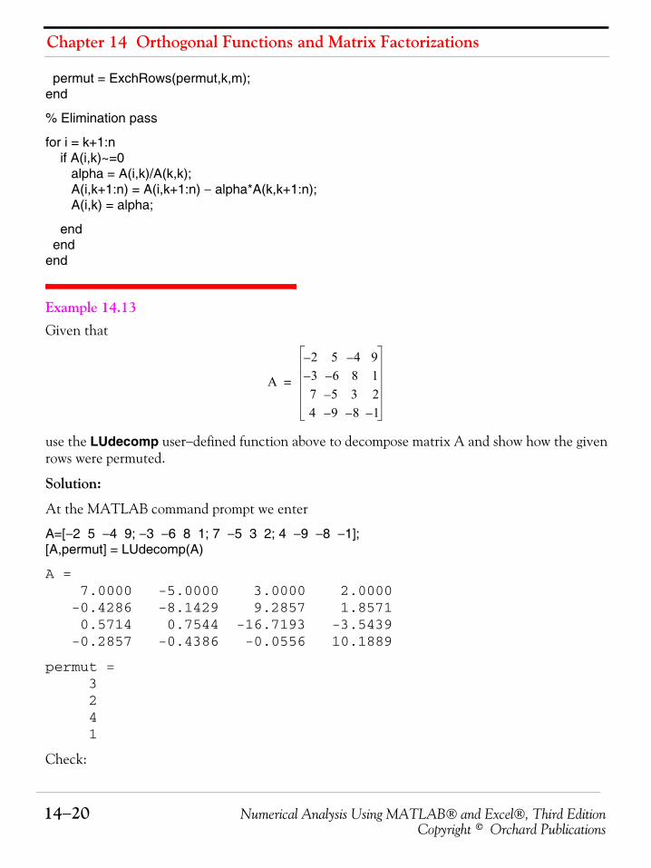
Chapter 14 Orthogonal Functions and Matrix Factorizations
14−20 Numerical Analysis Using MATLAB® and Excel®, Third EditionCopyright © Orchard Publications
permut = ExchRows(permut,k,m);end
% Elimination pass
for i = k+1:n if A(i,k)~=0 alpha = A(i,k)/A(k,k); A(i,k+1:n) = A(i,k+1:n) − alpha*A(k,k+1:n); A(i,k) = alpha;
end endend
Example 14.13 Given that
use the LUdecomp user−defined function above to decompose matrix A and show how the givenrows were permuted.
Solution:
At the MATLAB command prompt we enter
A=[−2 5 −4 9; −3 −6 8 1; 7 −5 3 2; 4 −9 −8 −1]; [A,permut] = LUdecomp(A)
A = 7.0000 -5.0000 3.0000 2.0000 -0.4286 -8.1429 9.2857 1.8571 0.5714 0.7544 -16.7193 -3.5439 -0.2857 -0.4386 -0.0556 10.1889
permut = 3 2 4 1
Check:
A
2– 5 4– 93– 6– 8 17 5– 3 24 9– 8– 1–
=
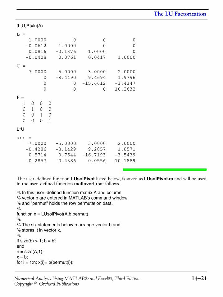
Numerical Analysis Using MATLAB® and Excel®, Third Edition 14−21Copyright © Orchard Publications
The LU Factorization
[L,U,P]=lu(A)
L = 1.0000 0 0 0 -0.0612 1.0000 0 0 0.0816 -0.1376 1.0000 0 -0.0408 0.0761 0.0417 1.0000
U = 7.0000 -5.0000 3.0000 2.0000 0 -8.4490 9.4694 1.9796 0 0 -15.6612 -3.4347 0 0 0 10.2632
P = 1 0 0 0 0 1 0 0 0 0 1 0 0 0 0 1
L*U
ans = 7.0000 -5.0000 3.0000 2.0000 -0.4286 -8.1429 9.2857 1.8571 0.5714 0.7544 -16.7193 -3.5439 -0.2857 -0.4386 -0.0556 10.1889
The user−defined function LUsolPivot listed below, is saved as LUsolPivot.m and will be usedin the user−defined function matInvert that follows.
% In this user−defined function matrix A and column % vector b are entered in MATLAB's command window% and “permut” holds the row permutation data.%function x = LUsolPivot(A,b,permut)%% The six statements below rearrange vector b and% stores it in vector x.% if size(b) > 1; b = b';endn = size(A,1);x = b;for i = 1:n; x(i)= b(permut(i));
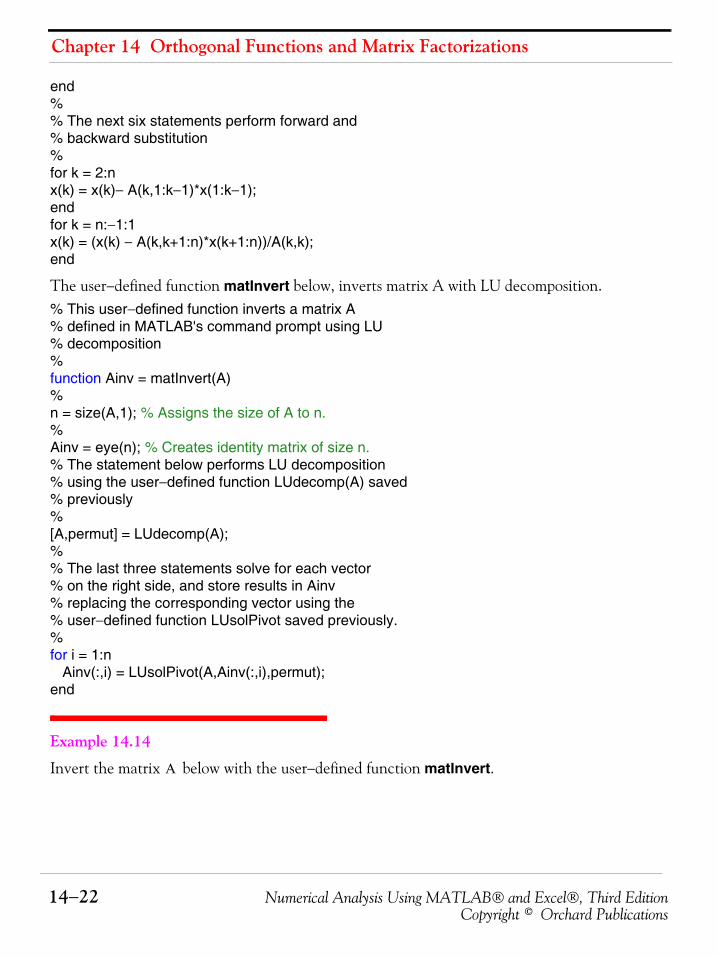
Chapter 14 Orthogonal Functions and Matrix Factorizations
14−22 Numerical Analysis Using MATLAB® and Excel®, Third EditionCopyright © Orchard Publications
end%% The next six statements perform forward and % backward substitution%for k = 2:nx(k) = x(k)− A(k,1:k−1)*x(1:k−1);endfor k = n:−1:1x(k) = (x(k) − A(k,k+1:n)*x(k+1:n))/A(k,k);end
The user−defined function matInvert below, inverts matrix A with LU decomposition.% This user−defined function inverts a matrix A% defined in MATLAB's command prompt using LU% decomposition%function Ainv = matInvert(A)%n = size(A,1); % Assigns the size of A to n.%Ainv = eye(n); % Creates identity matrix of size n.% The statement below performs LU decomposition% using the user−defined function LUdecomp(A) saved% previously%[A,permut] = LUdecomp(A);%% The last three statements solve for each vector% on the right side, and store results in Ainv % replacing the corresponding vector using the% user−defined function LUsolPivot saved previously.%for i = 1:n Ainv(:,i) = LUsolPivot(A,Ainv(:,i),permut);end
Example 14.14
Invert the matrix below with the user−defined function matInvert.A
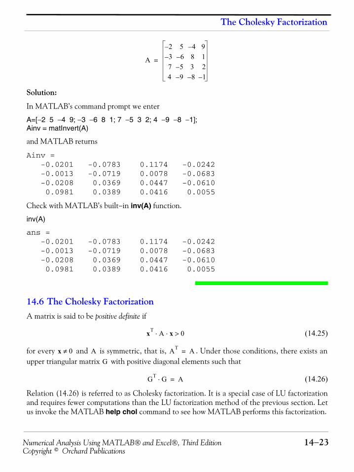
Numerical Analysis Using MATLAB® and Excel®, Third Edition 14−23Copyright © Orchard Publications
The Cholesky Factorization
Solution:
In MATLAB’s command prompt we enter
A=[−2 5 −4 9; −3 −6 8 1; 7 −5 3 2; 4 −9 −8 −1]; Ainv = matInvert(A)
and MATLAB returns
Ainv = -0.0201 -0.0783 0.1174 -0.0242 -0.0013 -0.0719 0.0078 -0.0683 -0.0208 0.0369 0.0447 -0.0610 0.0981 0.0389 0.0416 0.0055
Check with MATLAB’s built−in inv(A) function.
inv(A)
ans = -0.0201 -0.0783 0.1174 -0.0242 -0.0013 -0.0719 0.0078 -0.0683 -0.0208 0.0369 0.0447 -0.0610 0.0981 0.0389 0.0416 0.0055
14.6 The Cholesky FactorizationA matrix is said to be positive definite if
(14.25)
for every and is symmetric, that is, . Under those conditions, there exists anupper triangular matrix with positive diagonal elements such that
(14.26)
Relation (14.26) is referred to as Cholesky factorization. It is a special case of LU factorizationand requires fewer computations than the LU factorization method of the previous section. Letus invoke the MATLAB help chol command to see how MATLAB performs this factorization.
A
2– 5 4– 93– 6– 8 17 5– 3 24 9– 8– 1–
=
xT A x⋅ ⋅ 0>
x 0≠ A AT A=
G
GT G⋅ A=
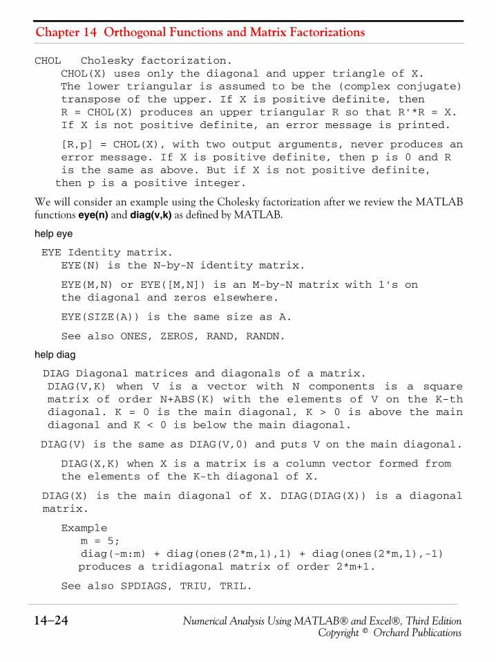
Chapter 14 Orthogonal Functions and Matrix Factorizations
14−24 Numerical Analysis Using MATLAB® and Excel®, Third EditionCopyright © Orchard Publications
CHOL Cholesky factorization. CHOL(X) uses only the diagonal and upper triangle of X. The lower triangular is assumed to be the (complex conjugate) transpose of the upper. If X is positive definite, then R = CHOL(X) produces an upper triangular R so that R'*R = X. If X is not positive definite, an error message is printed.
[R,p] = CHOL(X), with two output arguments, never produces an error message. If X is positive definite, then p is 0 and R is the same as above. But if X is not positive definite,
then p is a positive integer.
We will consider an example using the Cholesky factorization after we review the MATLABfunctions eye(n) and diag(v,k) as defined by MATLAB.
help eye
EYE Identity matrix. EYE(N) is the N-by-N identity matrix.
EYE(M,N) or EYE([M,N]) is an M-by-N matrix with 1's on the diagonal and zeros elsewhere.
EYE(SIZE(A)) is the same size as A.
See also ONES, ZEROS, RAND, RANDN.
help diag
DIAG Diagonal matrices and diagonals of a matrix.DIAG(V,K) when V is a vector with N components is a squarematrix of order N+ABS(K) with the elements of V on the K-thdiagonal. K = 0 is the main diagonal, K > 0 is above the maindiagonal and K < 0 is below the main diagonal.
DIAG(V) is the same as DIAG(V,0) and puts V on the main diagonal.
DIAG(X,K) when X is a matrix is a column vector formed from the elements of the K-th diagonal of X. DIAG(X) is the main diagonal of X. DIAG(DIAG(X)) is a diagonalmatrix.
Example m = 5; diag(-m:m) + diag(ones(2*m,1),1) + diag(ones(2*m,1),-1) produces a tridiagonal matrix of order 2*m+1. See also SPDIAGS, TRIU, TRIL.
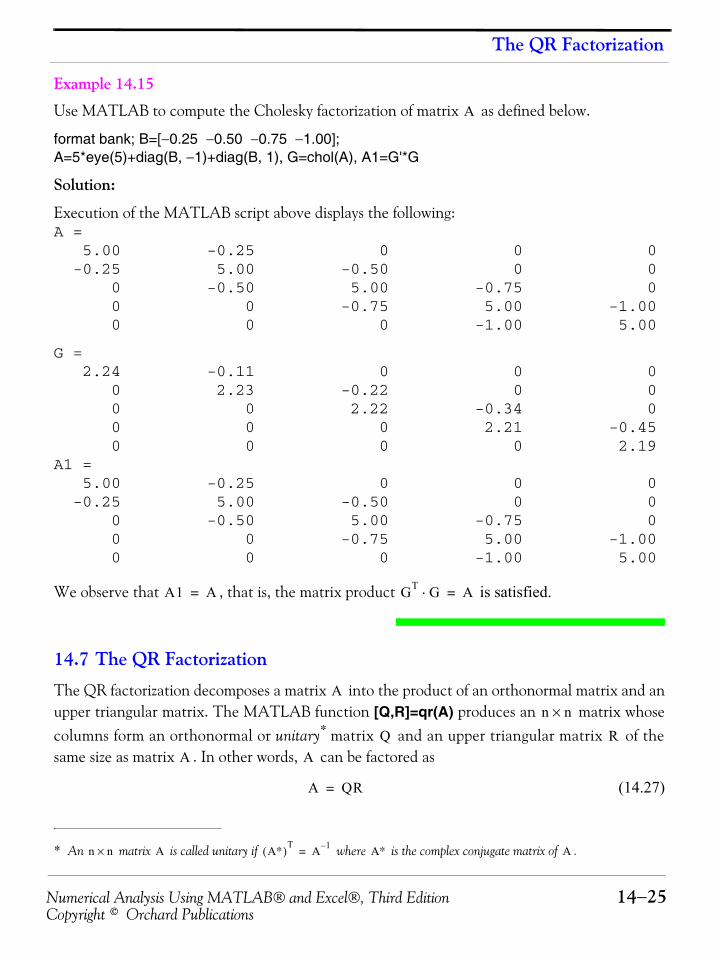
Numerical Analysis Using MATLAB® and Excel®, Third Edition 14−25Copyright © Orchard Publications
The QR Factorization
Example 14.15
Use MATLAB to compute the Cholesky factorization of matrix as defined below.
format bank; B=[−0.25 −0.50 −0.75 −1.00];A=5*eye(5)+diag(B, −1)+diag(B, 1), G=chol(A), A1=G'*G
Solution:
Execution of the MATLAB script above displays the following:A = 5.00 -0.25 0 0 0 -0.25 5.00 -0.50 0 0 0 -0.50 5.00 -0.75 0 0 0 -0.75 5.00 -1.00 0 0 0 -1.00 5.00
G = 2.24 -0.11 0 0 0 0 2.23 -0.22 0 0 0 0 2.22 -0.34 0 0 0 0 2.21 -0.45 0 0 0 0 2.19A1 = 5.00 -0.25 0 0 0 -0.25 5.00 -0.50 0 0 0 -0.50 5.00 -0.75 0 0 0 -0.75 5.00 -1.00 0 0 0 -1.00 5.00
We observe that , that is, the matrix product is satisfied.
14.7 The QR Factorization
The QR factorization decomposes a matrix into the product of an orthonormal matrix and anupper triangular matrix. The MATLAB function [Q,R]=qr(A) produces an matrix whosecolumns form an orthonormal or unitary* matrix and an upper triangular matrix of thesame size as matrix . In other words, can be factored as
(14.27)
* An matrix is called unitary if where is the complex conjugate matrix of .
A
A1 A= GT G⋅ A=
An n×
Q R
n n× A A∗( )T A 1–= A∗ A
A A
A QR=
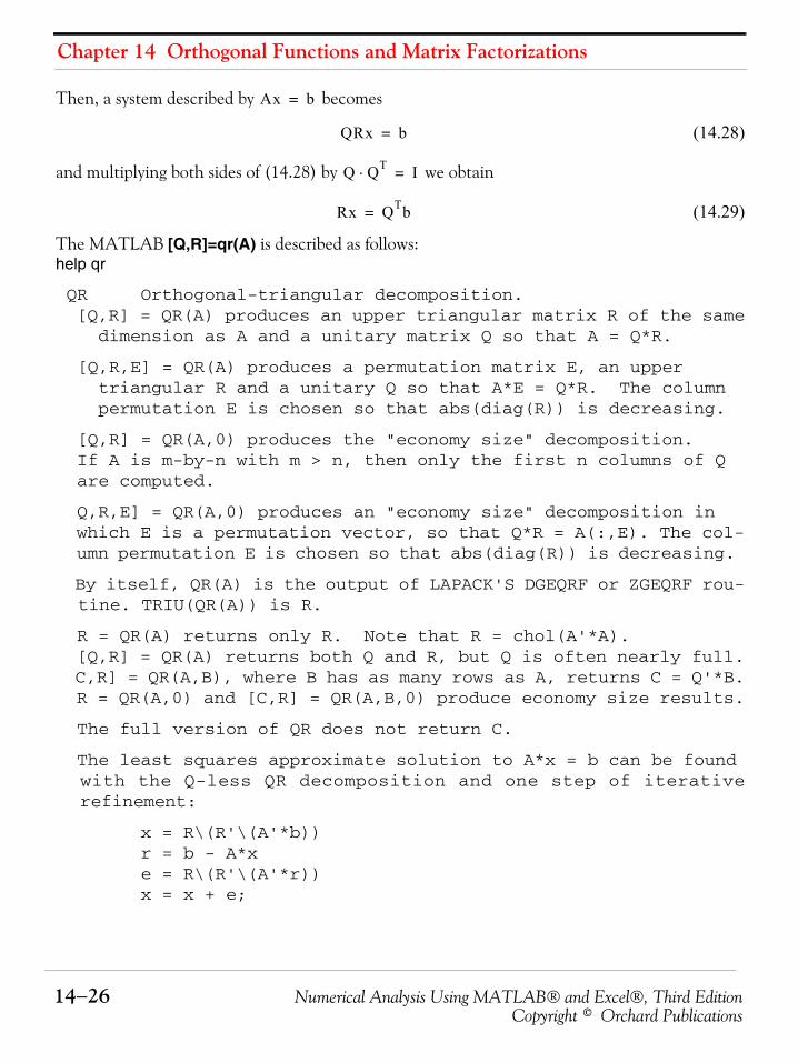
Chapter 14 Orthogonal Functions and Matrix Factorizations
14−26 Numerical Analysis Using MATLAB® and Excel®, Third EditionCopyright © Orchard Publications
Then, a system described by becomes
(14.28)
and multiplying both sides of (14.28) by we obtain
(14.29)
The MATLAB [Q,R]=qr(A) is described as follows:help qr
QR Orthogonal-triangular decomposition. [Q,R] = QR(A) produces an upper triangular matrix R of the same dimension as A and a unitary matrix Q so that A = Q*R. [Q,R,E] = QR(A) produces a permutation matrix E, an upper triangular R and a unitary Q so that A*E = Q*R. The column permutation E is chosen so that abs(diag(R)) is decreasing. [Q,R] = QR(A,0) produces the "economy size" decomposition. If A is m-by-n with m > n, then only the first n columns of Q are computed.
Q,R,E] = QR(A,0) produces an "economy size" decomposition in which E is a permutation vector, so that Q*R = A(:,E). The col-umn permutation E is chosen so that abs(diag(R)) is decreasing.
By itself, QR(A) is the output of LAPACK'S DGEQRF or ZGEQRF rou-
tine. TRIU(QR(A)) is R.
R = QR(A) returns only R. Note that R = chol(A'*A). [Q,R] = QR(A) returns both Q and R, but Q is often nearly full. C,R] = QR(A,B), where B has as many rows as A, returns C = Q'*B. R = QR(A,0) and [C,R] = QR(A,B,0) produce economy size results.
The full version of QR does not return C. The least squares approximate solution to A*x = b can be found with the Q-less QR decomposition and one step of iterative
refinement:
x = R\(R'\(A'*b)) r = b - A*x e = R\(R'\(A'*r)) x = x + e;
Ax b=
QRx b=
Q QT⋅ I=
Rx QTb=
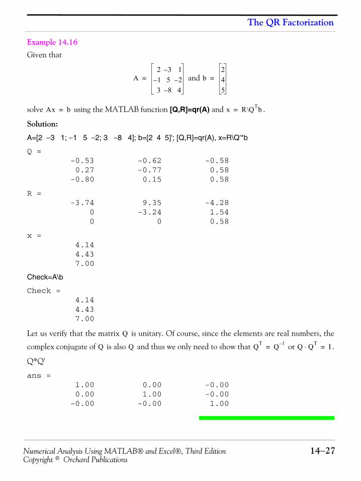
Numerical Analysis Using MATLAB® and Excel®, Third Edition 14−27Copyright © Orchard Publications
The QR Factorization
Example 14.16 Given that
and
solve using the MATLAB function [Q,R]=qr(A) and .
Solution:
A=[2 −3 1; −1 5 −2; 3 −8 4]; b=[2 4 5]'; [Q,R]=qr(A), x=R\Q'*b
Q = -0.53 -0.62 -0.58 0.27 -0.77 0.58 -0.80 0.15 0.58
R = -3.74 9.35 -4.28 0 -3.24 1.54 0 0 0.58
x = 4.14 4.43 7.00
Check=A\b
Check = 4.14 4.43 7.00
Let us verify that the matrix is unitary. Of course, since the elements are real numbers, the
complex conjugate of is also and thus we only need to show that or .
Q*Q'
ans = 1.00 0.00 -0.00 0.00 1.00 -0.00 -0.00 -0.00 1.00
A2 3– 11– 5 2–3 8– 4
= b245
=
Ax b= x R\QTb=
Q
Q Q QT Q 1–= Q QT⋅ I=
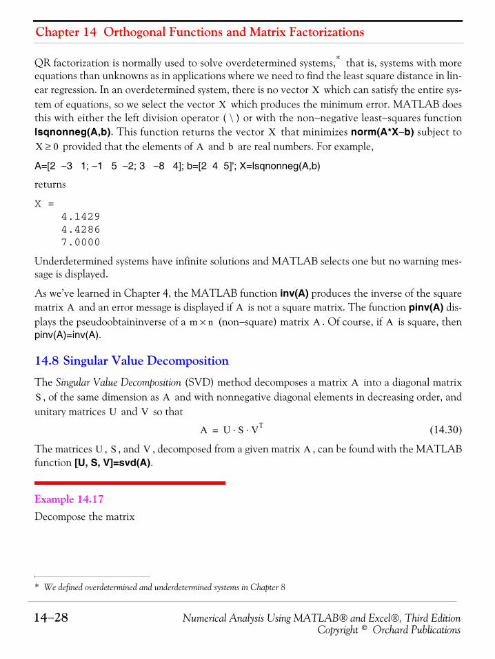
Chapter 14 Orthogonal Functions and Matrix Factorizations
14−28 Numerical Analysis Using MATLAB® and Excel®, Third EditionCopyright © Orchard Publications
QR factorization is normally used to solve overdetermined systems,* that is, systems with moreequations than unknowns as in applications where we need to find the least square distance in lin-ear regression. In an overdetermined system, there is no vector which can satisfy the entire sys-tem of equations, so we select the vector which produces the minimum error. MATLAB doesthis with either the left division operator ( \ ) or with the non−negative least−squares functionlsqnonneg(A,b). This function returns the vector that minimizes norm(A*X−b) subject to
provided that the elements of and are real numbers. For example,
A=[2 −3 1; −1 5 −2; 3 −8 4]; b=[2 4 5]'; X=lsqnonneg(A,b)
returns
X = 4.1429 4.4286 7.0000
Underdetermined systems have infinite solutions and MATLAB selects one but no warning mes-sage is displayed.
As we’ve learned in Chapter 4, the MATLAB function inv(A) produces the inverse of the squarematrix and an error message is displayed if is not a square matrix. The function pinv(A) dis-plays the pseudoobtaininverse of a (non−square) matrix . Of course, if is square, thenpinv(A)=inv(A).
14.8 Singular Value Decomposition
The Singular Value Decomposition (SVD) method decomposes a matrix into a diagonal matrix, of the same dimension as and with nonnegative diagonal elements in decreasing order, and
unitary matrices and so that
(14.30)
The matrices , , and , decomposed from a given matrix , can be found with the MATLABfunction [U, S, V]=svd(A).
Example 14.17 Decompose the matrix
* We defined overdetermined and underdetermined systems in Chapter 8
XX
XX 0≥ A b
A Am n× A A
AS A
U V
A U S VT⋅ ⋅=
U S V A
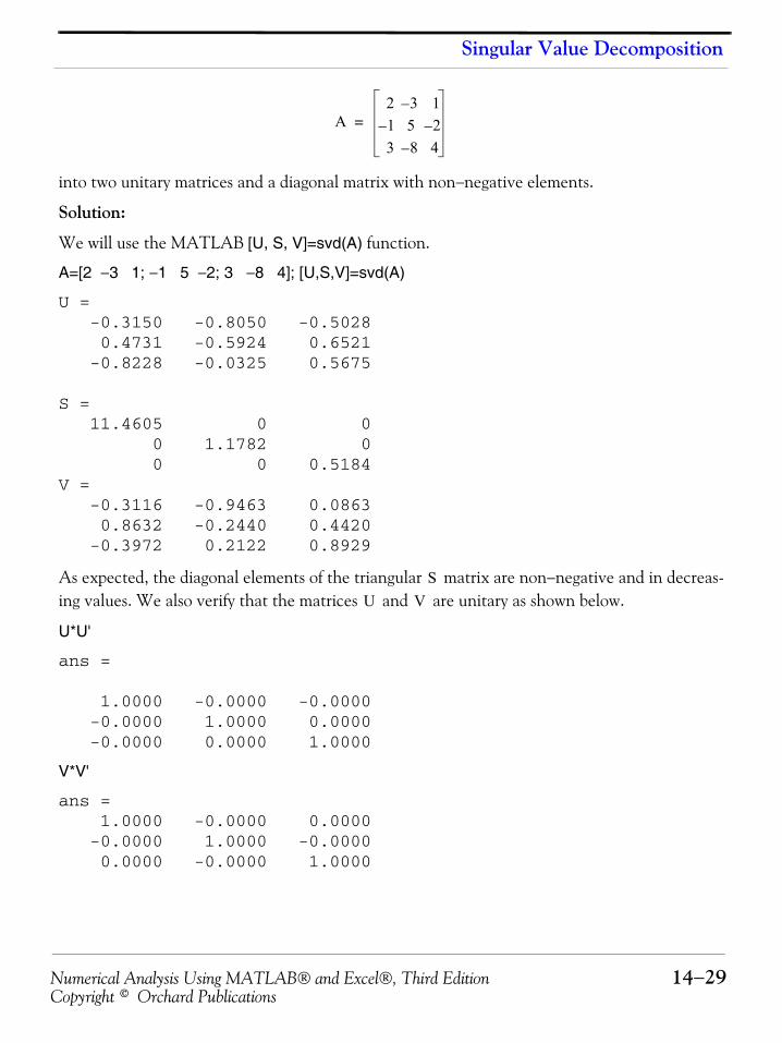
Numerical Analysis Using MATLAB® and Excel®, Third Edition 14−29Copyright © Orchard Publications
Singular Value Decomposition
into two unitary matrices and a diagonal matrix with non−negative elements.
Solution:
We will use the MATLAB [U, S, V]=svd(A) function.
A=[2 −3 1; −1 5 −2; 3 −8 4]; [U,S,V]=svd(A)
U = -0.3150 -0.8050 -0.5028 0.4731 -0.5924 0.6521 -0.8228 -0.0325 0.5675
S = 11.4605 0 0 0 1.1782 0 0 0 0.5184V = -0.3116 -0.9463 0.0863 0.8632 -0.2440 0.4420 -0.3972 0.2122 0.8929
As expected, the diagonal elements of the triangular matrix are non−negative and in decreas-ing values. We also verify that the matrices and are unitary as shown below. U*U'
ans =
1.0000 -0.0000 -0.0000 -0.0000 1.0000 0.0000 -0.0000 0.0000 1.0000
V*V'
ans = 1.0000 -0.0000 0.0000 -0.0000 1.0000 -0.0000 0.0000 -0.0000 1.0000
A2 3– 11– 5 2–3 8– 4
=
SU V
Chapter 14 Orthogonal Functions and Matrix Factorizations
14−30 Numerical Analysis Using MATLAB® and Excel®, Third EditionCopyright © Orchard Publications
14.9 Summary• Orthogonal functions are those which are perpendicular to each other.
• Two families of curves with the property that each member of either family cuts every memberof the other family at right angles are said to be orthogonal trajectories of each other.
• The inner (dot) product of two vectors and isa scalar defined as
• If the dot product of two vectors and is zero, these vector are said to be orthogonal toeach other.
• The magnitude of a vector , denoted as , is defined as . A uniqueunit vector is obtained by dividing each component of by the magnitude and this pro-cess is referred to as normalization.
• A basis that consists of mutually orthogonal vectors is referred to as an orthogonal basis. Ifthese vectors are also unit vectors, the basis is called orthonormal basis.
• If the column (or row) vectors of a square matrix are mutually orthogonal unit vectors, the
matrix is said to be orthogonal and where is the transpose of and is theidentity matrix.
• We can find an orthonormal set of eigenvectors in a matrix easily from the eigenvaluesbut the computations for finding orthonormal sets of eigenvectors for larger size ( orhigher) matrices using the above procedure becomes quite involved. A simpler procedure isthe Gram−Schmidt orthogonalization procedure which we will discuss on the next section.
• The LU factorization method decomposes a matrix into a lower triangular matrix and anupper triangular matrix so that . The MATLAB function [L,U]=lu(A) decomposesthe matrix into a lower triangular matrix and an upper triangular matrix .
• A matrix is said to be positive definite if for every and is symmetric, that
is, . Under those conditions, there exists an upper triangular matrix with positive
diagonal elements such that . This process is referred to as the Cholesky factoriza-tion.
• The QR factorization decomposes a matrix into the product of an orthonormal matrix andan upper triangular matrix. The MATLAB function [Q,R]=qr(A) produces an matrixwhose columns form an orthonormal or unitary matrix and an upper triangular matrix ofthe same size as matrix .
X x1 x2 x3 … xn[ ]= Y y1 y2 y3 … yn[ ]=
X Y⋅ x1 y1 x2 y2 x3 y3 … xn yn+ + + +=
X1 X2
X X X x12 x2
2 … xn2+ + +=
U X X
A
A A AT⋅ I= AT A I
2 2×3 3×
A LU A L U⋅=
A L U
xT A x⋅ ⋅ 0> x 0≠ A
AT A= G
GT G⋅ A=
An n×
Q RA

Numerical Analysis Using MATLAB® and Excel®, Third Edition 14−31Copyright © Orchard Publications
Summary
• The Singular Value Decomposition (SVD) method decomposes a matrix into a diagonalmatrix , of the same dimension as and with nonnegative diagonal elements in decreasing
order, and unitary matrices and so that . The matrices , , and ,decomposed from a given matrix , can be found with the MATLAB function [U, S,V]=svd(A).
AS A
U V A U S VT⋅ ⋅= U S VA
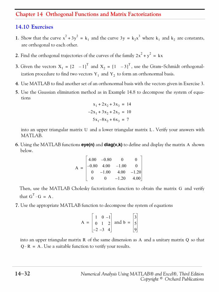
Chapter 14 Orthogonal Functions and Matrix Factorizations
14−32 Numerical Analysis Using MATLAB® and Excel®, Third EditionCopyright © Orchard Publications
14.10 Exercises
1. Show that the curve and the curve where and are constants,are orthogonal to each other.
2. Find the orthogonal trajectories of the curves of the family
3. Given the vectors and , use the Gram−Schmidt orthogonal-ization procedure to find two vectors and to form an orthonormal basis.
4. Use MATLAB to find another set of an orthonormal basis with the vectors given in Exercise 3.
5. Use the Gaussian elimination method as in Example 14.8 to decompose the system of equa-tions
into an upper triangular matrix and a lower triangular matrix . Verify your answers withMATLAB.
6. Using the MATLAB functions eye(n) and diag(v,k) to define and display the matrix shownbelow.
Then, use the MATLAB Cholesky factorization function to obtain the matrix and verify
that .
7. Use the appropriate MATLAB function to decompose the system of equations
and
into an upper triangular matrix of the same dimension as and a unitary matrix so that. Use a suitable function to verify your results.
x2 3y2+ k1= 3y k2x3= k1 k2
2x2 y2+ kx=
X1 2 1–[ ]T= X2 1 3–[ ]T=
Y1 Y2
x1 2x2 3x3+ + 14=
2x– 1 3x2 2x3+ + 10=
5x1 8– x2 6x3+ 7=
U L
A
A
4.00 0.80– 0 00.80– 4.00 1.00– 00 1.00– 4.00 1.20–0 0 1.20– 4.00
=
G
GT G⋅ A=
A1 0 1–0 1 22– 3– 4
= b359
=
R A QQ R⋅ A=

Numerical Analysis Using MATLAB® and Excel®, Third Edition 14−33Copyright © Orchard Publications
Exercises
8. Use the appropriate MATLAB function to decompose the matrix given as
into a diagonal matrix of the same dimension as and with non−negative diagonal ele-
ments in decreasing order and unitary matrices and so that .
A
A1 0 1–0 1 22– 3– 4
=
S A
U V U S VT⋅ ⋅ A=
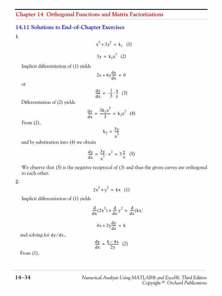
Chapter 14 Orthogonal Functions and Matrix Factorizations
14−34 Numerical Analysis Using MATLAB® and Excel®, Third EditionCopyright © Orchard Publications
14.11 Solutions to End−of−Chapter Exercises1.
(1)
(2)
Implicit differentiation of (1) yields
or
(3)
Differentiation of (2) yields
(4)
From (2),
and by substitution into (4) we obtain
(5)
We observe that (5) is the negative reciprocal of (3) and thus the given curves are orthogonalto each other.
2.
(1)
Implicit differentiation of (1) yields
and solving for ,
(2)
From (1),
x2 3y2+ k1=
3y k2x3=
2x 6ydydx------+ 0=
dydx------ 1
3--- x
y---⋅–=
dydx------
3k2x2
3-------------- k2x2= =
k23yx3------=
dydx------ 3y
x3------ x2⋅ 3 y
x---= =
2x2 y2+ kx=
ddx------ 2x2( ) d
dx------ y2+
ddx------ kx( )=
4x 2ydydx------+ k=
dy dx⁄dydx------ k 4x–
2y---------------=
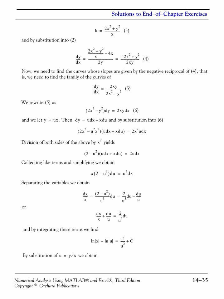
Numerical Analysis Using MATLAB® and Excel®, Third Edition 14−35Copyright © Orchard Publications
Solutions to End−of−Chapter Exercises
(3)
and by substitution into (2)
(4)
Now, we need to find the curves whose slopes are given by the negative reciprocal of (4), thatis, we need to find the family of the curves of
(5)
We rewrite (5) as
(6)
and we let . Then, and by substitution into (6)
Division of both sides of the above by yields
Collecting like terms and simplifying we obtain
Separating the variables we obtain
or
and by integrating these terms we find
By substitution of we obtain
k 2x2 y2+x
--------------------=
dydx------
2x2 y2+x
-------------------- 4x–
2y--------------------------------- 2x2– y2+
2xy-------------------------= =
dydx------ 2xy
2x2 y2–--------------------=
2x2 y2–( )dy 2xydx=
y ux= dy udx xdu+=
2x2 u2x2–( ) udx xdu+( ) 2x2udx=
x2
2 u2–( ) udx xdu+( ) 2udx=
x 2 u2–( )du u3dx=
dxx
------ 2 u2–( )u3
-------------------du 2u3-----du du
u------–= =
dxx
------ duu
------+2u3-----du=
xln uln+ 1–
u2------ C+=
u y x⁄=
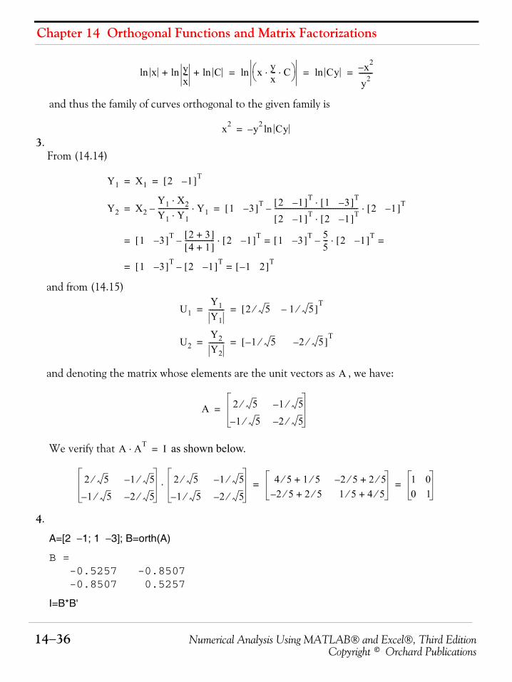
Chapter 14 Orthogonal Functions and Matrix Factorizations
14−36 Numerical Analysis Using MATLAB® and Excel®, Third EditionCopyright © Orchard Publications
and thus the family of curves orthogonal to the given family is
3.From (14.14)
and from (14.15)
and denoting the matrix whose elements are the unit vectors as , we have:
We verify that as shown below.
4.
A=[2 −1; 1 −3]; B=orth(A)
B = -0.5257 -0.8507 -0.8507 0.5257
I=B*B'
xln yx---ln Cln+ + x y
x--- C⋅ ⋅⎝ ⎠
⎛ ⎞ln Cyln x2–
y2--------= = =
x2 y2 Cyln–=
Y1 X1 2 1–[ ]T= =
Y2 X2Y1 X2⋅Y1 Y1⋅------------------ Y1⋅– 1 3–[ ]T 2 1–[ ]T 1 3–[ ]T⋅
2 1–[ ]T 2 1–[ ]T⋅------------------------------------------------ 2 1–[ ]T⋅–= =
1 3–[ ]T 2 3+[ ]4 1+[ ]
----------------- 2 1–[ ]T⋅– 1 3–[ ]T 55--- 2 1–[ ]T⋅–= ==
1 3–[ ]T 2 1–[ ]T– 1– 2[ ]T==
U1Y1Y1--------- 2 5⁄ 1– 5⁄[ ]
T= =
U2Y2Y2--------- 1– 5 ⁄ 2– 5⁄[ ]
T= =
A
A 2 5⁄ 1– 5⁄
1– 5⁄ 2– 5⁄=
A AT⋅ I=
2 5⁄ 1– 5⁄
1– 5⁄ 2– 5⁄
2 5⁄ 1– 5⁄
1– 5⁄ 2– 5⁄⋅ 4 5⁄ 1 5⁄+ 2– 5⁄ 2 5⁄+
2– 5⁄ 2 5⁄+ 1 5⁄ 4 5⁄+1 00 1
= =
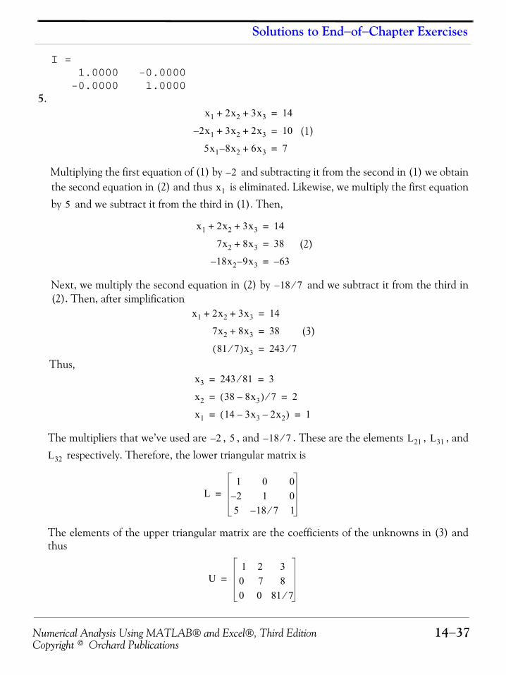
Numerical Analysis Using MATLAB® and Excel®, Third Edition 14−37Copyright © Orchard Publications
Solutions to End−of−Chapter Exercises
I = 1.0000 -0.0000 -0.0000 1.0000
5.
(1)
Multiplying the first equation of (1) by and subtracting it from the second in (1) we obtainthe second equation in (2) and thus is eliminated. Likewise, we multiply the first equationby and we subtract it from the third in (1). Then,
(2)
Next, we multiply the second equation in (2) by and we subtract it from the third in(2). Then, after simplification
(3)
Thus,
The multipliers that we’ve used are , , and . These are the elements , , and respectively. Therefore, the lower triangular matrix is
The elements of the upper triangular matrix are the coefficients of the unknowns in (3) andthus
x1 2x2 3x3+ + 14=
2x– 1 3x2 2x3+ + 10=
5x1 8– x2 6x3+ 7=
2–
x1
5
x1 2x2 3x3+ + 14=
7x2 8x3+ 38=
18– x2 9– x3 63–=
18 7⁄–
x1 2x2 3x3+ + 14=
7x2 8x3+ 38=
81 7⁄( )x3 243 7⁄=
x3 243 81⁄ 3= =
x2 38 8x3–( ) 7⁄ 2= =
x1 14 3x3 2x2––( ) 1= =
2– 5 18– 7⁄ L21 L31
L32
L1 0 02– 1 0
5 18 7⁄– 1
=
U1 2 30 7 80 0 81 7⁄
=
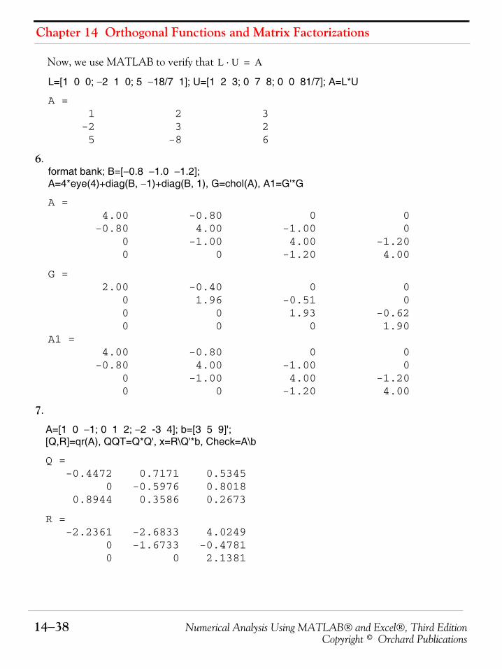
Chapter 14 Orthogonal Functions and Matrix Factorizations
14−38 Numerical Analysis Using MATLAB® and Excel®, Third EditionCopyright © Orchard Publications
Now, we use MATLAB to verify that
L=[1 0 0; −2 1 0; 5 −18/7 1]; U=[1 2 3; 0 7 8; 0 0 81/7]; A=L*U
A = 1 2 3 -2 3 2 5 -8 6
6.format bank; B=[−0.8 −1.0 −1.2];A=4*eye(4)+diag(B, −1)+diag(B, 1), G=chol(A), A1=G'*G
A = 4.00 -0.80 0 0 -0.80 4.00 -1.00 0 0 -1.00 4.00 -1.20 0 0 -1.20 4.00
G = 2.00 -0.40 0 0 0 1.96 -0.51 0 0 0 1.93 -0.62 0 0 0 1.90A1 =
4.00 -0.80 0 0 -0.80 4.00 -1.00 0 0 -1.00 4.00 -1.20 0 0 -1.20 4.00
7.
A=[1 0 −1; 0 1 2; −2 -3 4]; b=[3 5 9]';[Q,R]=qr(A), QQT=Q*Q', x=R\Q'*b, Check=A\b
Q = -0.4472 0.7171 0.5345 0 -0.5976 0.8018 0.8944 0.3586 0.2673
R = -2.2361 -2.6833 4.0249 0 -1.6733 -0.4781 0 0 2.1381
L U⋅ A=
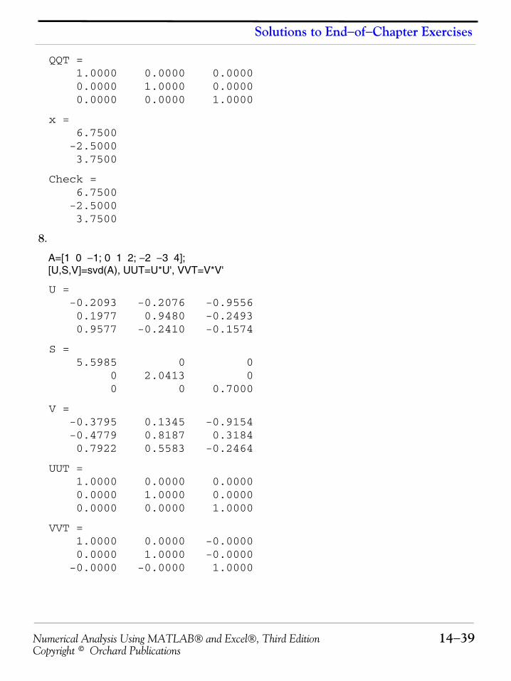
Numerical Analysis Using MATLAB® and Excel®, Third Edition 14−39Copyright © Orchard Publications
Solutions to End−of−Chapter Exercises
QQT = 1.0000 0.0000 0.0000 0.0000 1.0000 0.0000 0.0000 0.0000 1.0000
x = 6.7500 -2.5000 3.7500
Check = 6.7500 -2.5000 3.7500
8.
A=[1 0 −1; 0 1 2; −2 −3 4];[U,S,V]=svd(A), UUT=U*U', VVT=V*V'
U = -0.2093 -0.2076 -0.9556 0.1977 0.9480 -0.2493 0.9577 -0.2410 -0.1574
S = 5.5985 0 0 0 2.0413 0 0 0 0.7000
V = -0.3795 0.1345 -0.9154 -0.4779 0.8187 0.3184 0.7922 0.5583 -0.2464
UUT = 1.0000 0.0000 0.0000 0.0000 1.0000 0.0000 0.0000 0.0000 1.0000
VVT = 1.0000 0.0000 -0.0000 0.0000 1.0000 -0.0000 -0.0000 -0.0000 1.0000
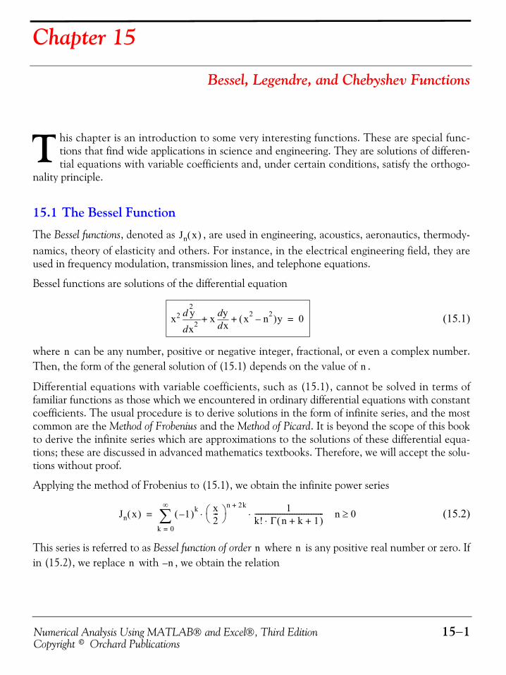
Numerical Analysis Using MATLAB® and Excel®, Third Edition 15−1Copyright © Orchard Publications
Chapter 15
Bessel, Legendre, and Chebyshev Functions
his chapter is an introduction to some very interesting functions. These are special func-tions that find wide applications in science and engineering. They are solutions of differen-tial equations with variable coefficients and, under certain conditions, satisfy the orthogo-
nality principle.
15.1 The Bessel Function
The Bessel functions, denoted as , are used in engineering, acoustics, aeronautics, thermody-namics, theory of elasticity and others. For instance, in the electrical engineering field, they areused in frequency modulation, transmission lines, and telephone equations.
Bessel functions are solutions of the differential equation
(15.1)
where can be any number, positive or negative integer, fractional, or even a complex number.Then, the form of the general solution of (15.1) depends on the value of .
Differential equations with variable coefficients, such as (15.1), cannot be solved in terms offamiliar functions as those which we encountered in ordinary differential equations with constantcoefficients. The usual procedure is to derive solutions in the form of infinite series, and the mostcommon are the Method of Frobenius and the Method of Picard. It is beyond the scope of this bookto derive the infinite series which are approximations to the solutions of these differential equa-tions; these are discussed in advanced mathematics textbooks. Therefore, we will accept the solu-tions without proof.
Applying the method of Frobenius to (15.1), we obtain the infinite power series
(15.2)
This series is referred to as Bessel function of order where is any positive real number or zero. Ifin (15.2), we replace with , we obtain the relation
T
Jn x( )
x2
x2
2
d
d y x xddy x2 n2–( )y+ + 0=
nn
Jn x( ) 1–( )k
k 0=
∞
∑x2---⎝ ⎠
⎛ ⎞ n 2k+ 1k! Γ n k 1+ +( )⋅----------------------------------------⋅ ⋅ n 0≥=
n nn n–
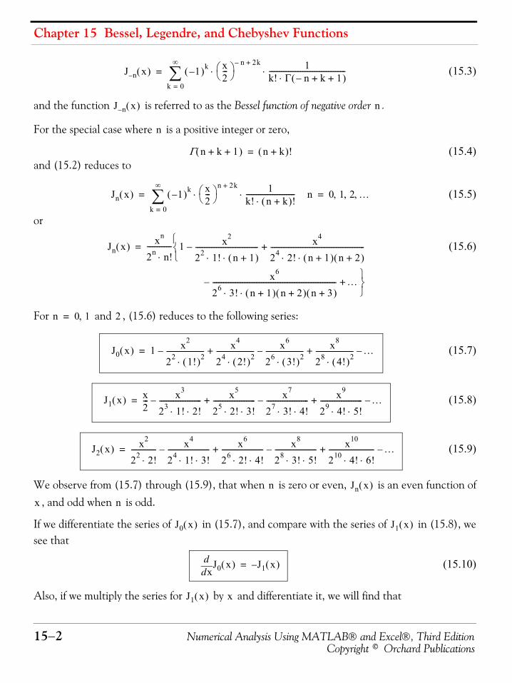
Chapter 15 Bessel, Legendre, and Chebyshev Functions
15−2 Numerical Analysis Using MATLAB® and Excel®, Third EditionCopyright © Orchard Publications
(15.3)
and the function is referred to as the Bessel function of negative order .
For the special case where is a positive integer or zero,
(15.4)and (15.2) reduces to
(15.5)
or
(15.6)
For and , (15.6) reduces to the following series:
(15.7)
(15.8)
(15.9)
We observe from (15.7) through (15.9), that when is zero or even, is an even function of, and odd when is odd.
If we differentiate the series of in (15.7), and compare with the series of in (15.8), wesee that
(15.10)
Also, if we multiply the series for by and differentiate it, we will find that
J n– x( ) 1–( )k
k 0=
∞
∑x2---⎝ ⎠
⎛ ⎞ n– 2k+ 1k! Γ n– k 1+ +( )⋅--------------------------------------------⋅ ⋅ =
J n– x( ) n
n
Γ n k 1+ +( ) n k+( )!=
Jn x( ) 1–( )k
k 0=
∞
∑x2---⎝ ⎠
⎛ ⎞ n 2k+ 1k! n k+( )!⋅----------------------------⋅ ⋅ n 0 1 2 …, , ,= =
Jn x( ) xn
2n n!⋅-------------- 1 x2
22 1! n 1+( )⋅ ⋅------------------------------------– x4
24 2! n 1+( ) n 2+( )⋅ ⋅------------------------------------------------------
x6
26 3! n 1+( ) n 2+( ) n 3+( )⋅ ⋅-----------------------------------------------------------------------– …
+
+
⎩
⎭
⎨
⎬
⎧
⎫
=
n 0 1,= 2
J0 x( ) 1 x2
22 1!( )2⋅----------------------– x4
24 2!( )2⋅---------------------- x6
26 3!( )2⋅---------------------- x8
28 4!( )2⋅---------------------- …–+–+=
J1 x( ) x2--- x3
23 1! 2!⋅ ⋅------------------------– x5
25 2! 3!⋅ ⋅------------------------ x7
27 3! 4!⋅ ⋅------------------------ x9
29 4! 5!⋅ ⋅------------------------ …–+–+=
J2 x( ) x2
22 2!⋅-------------- x4
24 1! 3!⋅ ⋅------------------------– x6
26 2! 4!⋅ ⋅------------------------ x8
28 3! 5!⋅ ⋅------------------------ x10
210 4! 6!⋅ ⋅-------------------------- …–+–+=
n Jn x( )
x n
J0 x( ) J1 x( )
xdd J0 x( ) J1 x( )–=
J1 x( ) x
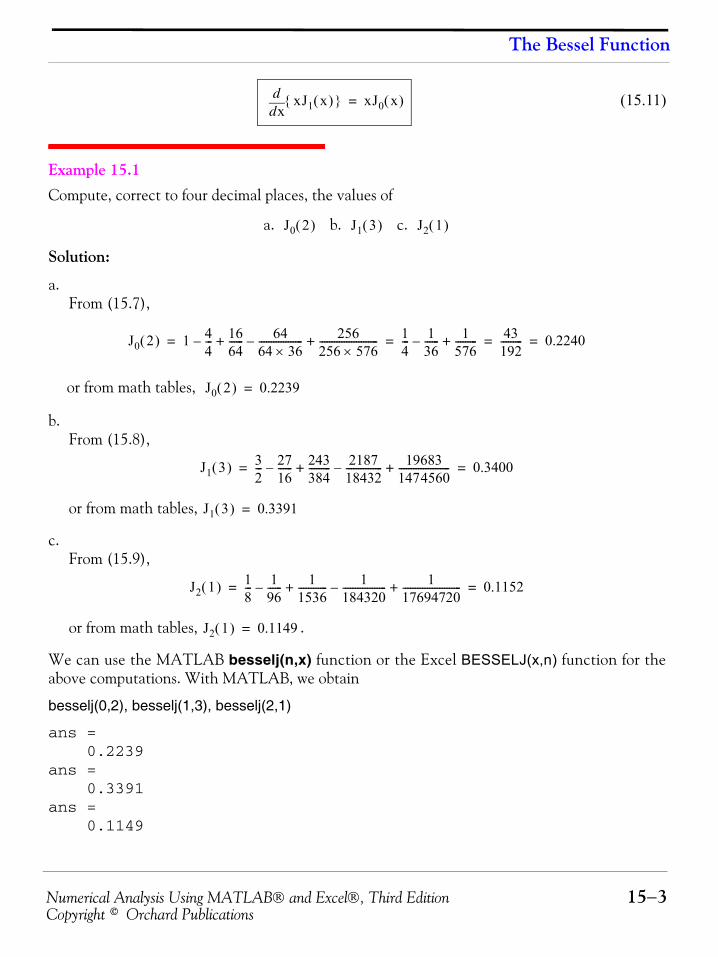
Numerical Analysis Using MATLAB® and Excel®, Third Edition 15−3Copyright © Orchard Publications
The Bessel Function
(15.11)
Example 15.1 Compute, correct to four decimal places, the values of
a. b. c.
Solution:
a.From (15.7),
or from math tables,
b.From (15.8),
or from math tables,
c.From (15.9),
or from math tables, .
We can use the MATLAB besselj(n,x) function or the Excel BESSELJ(x,n) function for theabove computations. With MATLAB, we obtain
besselj(0,2), besselj(1,3), besselj(2,1)
ans = 0.2239ans = 0.3391ans = 0.1149
xdd xJ1 x( ){ } xJ0 x( )=
J0 2( ) J1 3( ) J2 1( )
J0 2( ) 1 44---– 16
64------ 64
64 36×------------------– 256
256 576×------------------------+ + 1
4--- 1
36------– 1
576---------+ 43
192--------- 0.2240= = = =
J0 2( ) 0.2239=
J1 3( ) 32--- 27
16------– 243
384--------- 2187
18432---------------– 19683
1474560---------------------+ + 0.3400= =
J1 3( ) 0.3391=
J2 1( ) 18--- 1
96------– 1
1536------------ 1
184320------------------– 1
17694720------------------------+ + 0.1152= =
J2 1( ) 0.1149=
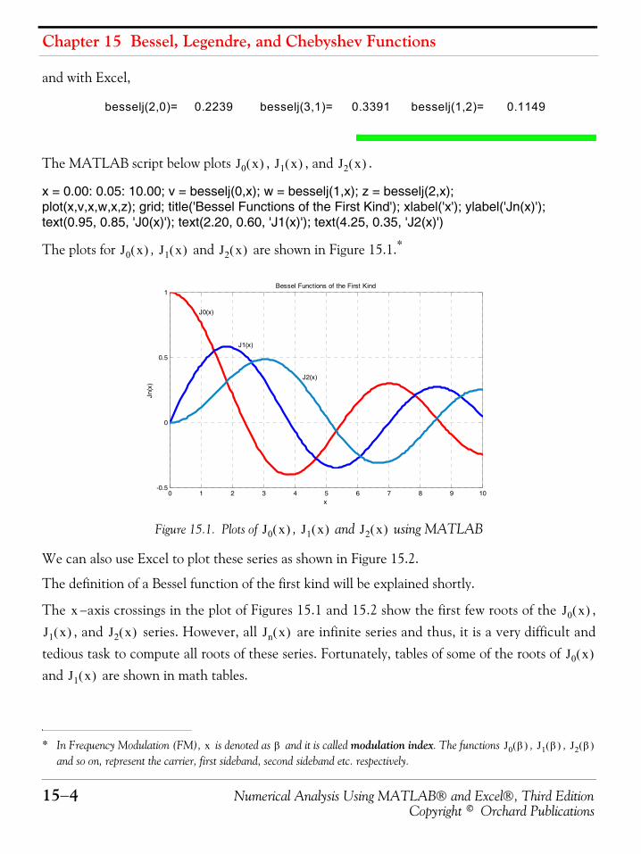
Chapter 15 Bessel, Legendre, and Chebyshev Functions
15−4 Numerical Analysis Using MATLAB® and Excel®, Third EditionCopyright © Orchard Publications
and with Excel,
The MATLAB script below plots , , and .
x = 0.00: 0.05: 10.00; v = besselj(0,x); w = besselj(1,x); z = besselj(2,x);plot(x,v,x,w,x,z); grid; title('Bessel Functions of the First Kind'); xlabel('x'); ylabel('Jn(x)');text(0.95, 0.85, 'J0(x)'); text(2.20, 0.60, 'J1(x)'); text(4.25, 0.35, 'J2(x)')
The plots for , and are shown in Figure 15.1.*
Figure 15.1. Plots of , and using MATLAB
We can also use Excel to plot these series as shown in Figure 15.2.
The definition of a Bessel function of the first kind will be explained shortly.
The −axis crossings in the plot of Figures 15.1 and 15.2 show the first few roots of the ,, and series. However, all are infinite series and thus, it is a very difficult and
tedious task to compute all roots of these series. Fortunately, tables of some of the roots of and are shown in math tables.
* In Frequency Modulation (FM), is denoted as and it is called modulation index. The functions , , and so on, represent the carrier, first sideband, second sideband etc. respectively.
besselj(2,0)= 0.2239 besselj(3,1)= 0.3391 besselj(1,2)= 0.1149
J0 x( ) J1 x( ) J2 x( )
J0 x( ) J1 x( ) J2 x( )
x β J0 β( ) J1 β( ) J2 β( )
0 1 2 3 4 5 6 7 8 9 10-0.5
0
0.5
1Bessel Functions of the First Kind
x
Jn(x
)
J0(x)
J1(x)
J2(x)
J0 x( ) J1 x( ) J2 x( )
x J0 x( )
J1 x( ) J2 x( ) Jn x( )
J0 x( )
J1 x( )
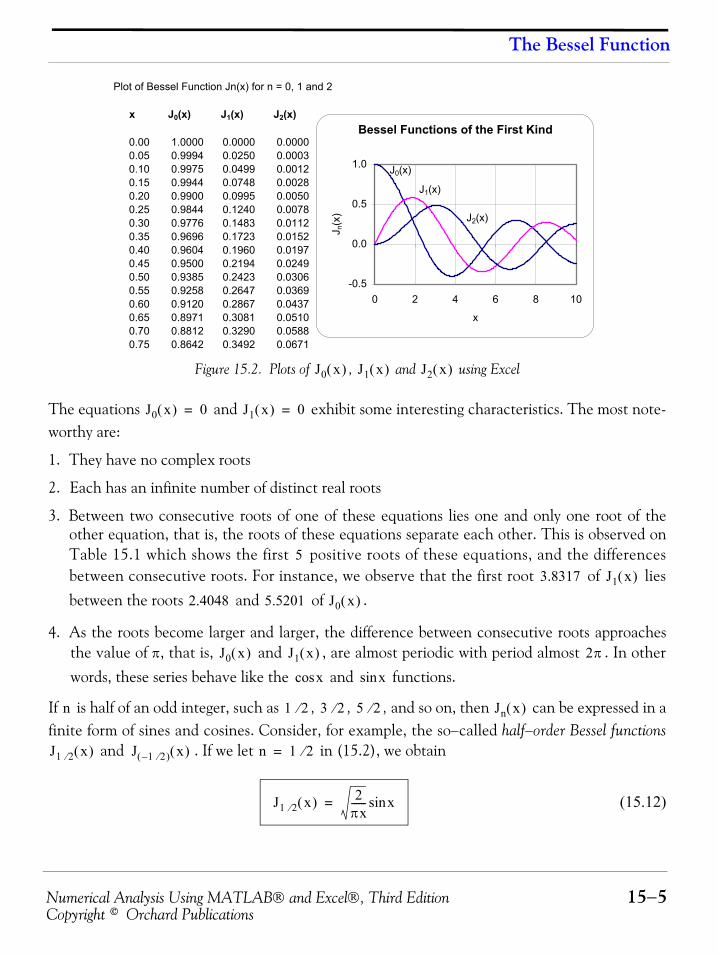
Numerical Analysis Using MATLAB® and Excel®, Third Edition 15−5Copyright © Orchard Publications
The Bessel Function
Figure 15.2. Plots of , and using Excel
The equations and exhibit some interesting characteristics. The most note-worthy are:
1. They have no complex roots
2. Each has an infinite number of distinct real roots
3. Between two consecutive roots of one of these equations lies one and only one root of theother equation, that is, the roots of these equations separate each other. This is observed onTable 15.1 which shows the first positive roots of these equations, and the differencesbetween consecutive roots. For instance, we observe that the first root of liesbetween the roots and of .
4. As the roots become larger and larger, the difference between consecutive roots approachesthe value of π, that is, and , are almost periodic with period almost . In otherwords, these series behave like the and functions.
If is half of an odd integer, such as , , , and so on, then can be expressed in afinite form of sines and cosines. Consider, for example, the so−called half−order Bessel functions
and . If we let in (15.2), we obtain
(15.12)
Plot of Bessel Function Jn(x) for n = 0, 1 and 2
x J0(x) J1(x) J2(x)
0.00 1.0000 0.0000 0.00000.05 0.9994 0.0250 0.00030.10 0.9975 0.0499 0.00120.15 0.9944 0.0748 0.00280.20 0.9900 0.0995 0.00500.25 0.9844 0.1240 0.00780.30 0.9776 0.1483 0.01120.35 0.9696 0.1723 0.01520.40 0.9604 0.1960 0.01970.45 0.9500 0.2194 0.02490.50 0.9385 0.2423 0.03060.55 0.9258 0.2647 0.03690.60 0.9120 0.2867 0.04370.65 0.8971 0.3081 0.05100.70 0.8812 0.3290 0.05880.75 0.8642 0.3492 0.0671
Bessel Functions of the First Kind
-0.5
0.0
0.5
1.0
0 2 4 6 8 10
x
J n(x
)
J0(x)
J1(x)
J2(x)
J0 x( ) J1 x( ) J2 x( )
J0 x( ) 0= J1 x( ) 0=
53.8317 J1 x( )
2.4048 5.5201 J0 x( )
J0 x( ) J1 x( ) 2π
xcos xsin
n 1 2⁄ 3 2⁄ 5 2⁄ Jn x( )
J1 2⁄ x( ) J 1 2⁄–( ) x( ) n 1 2⁄=
J1 2⁄ x( ) 2πx------ xsin=
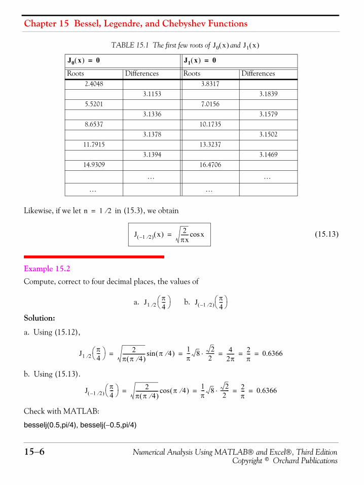
Chapter 15 Bessel, Legendre, and Chebyshev Functions
15−6 Numerical Analysis Using MATLAB® and Excel®, Third EditionCopyright © Orchard Publications
Likewise, if we let in (15.3), we obtain
(15.13)
Example 15.2 Compute, correct to four decimal places, the values of
a. b.
Solution:
a. Using (15.12),
b. Using (15.13).
Check with MATLAB:
besselj(0.5,pi/4), besselj(−0.5,pi/4)
TABLE 15.1 The first few roots of and
Roots Differences Roots Differences2.4048 3.8317
3.1153 3.18395.5201 7.0156
3.1336 3.15798.6537 10.1735
3.1378 3.150211.7915 13.3237
3.1394 3.146914.9309 16.4706
J0 x( ) J1 x( )
J0 x( ) 0= J1 x( ) 0=
… …
… …
n 1 2⁄=
J 1 2⁄–( ) x( ) 2πx------ xcos=
J1 2⁄π4---⎝ ⎠
⎛ ⎞ J 1 2⁄–( )π4---⎝ ⎠
⎛ ⎞
J1 2⁄π4---⎝ ⎠
⎛ ⎞ 2π π 4⁄( )------------------ π 4⁄( )sin 1
π--- 8 2
2-------⋅ 4
2π------ 2
π--- 0.6366= = = = =
J 1 2⁄–( )π4---⎝ ⎠
⎛ ⎞ 2π π 4⁄( )------------------ π 4⁄( )cos 1
π--- 8 2
2-------⋅ 2
π--- 0.6366= = = =
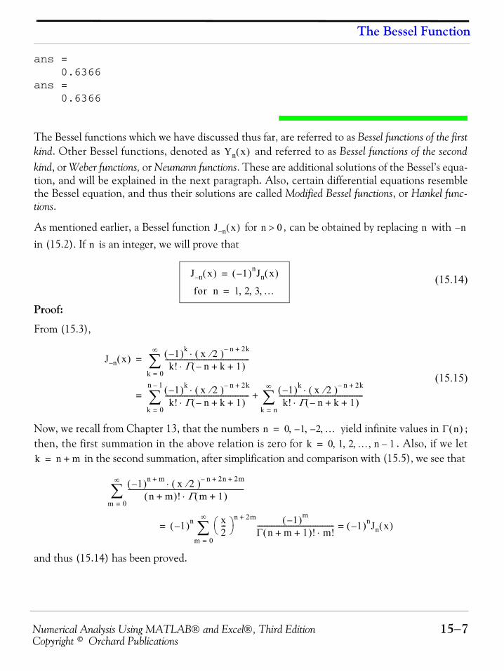
Numerical Analysis Using MATLAB® and Excel®, Third Edition 15−7Copyright © Orchard Publications
The Bessel Function
ans = 0.6366ans = 0.6366
The Bessel functions which we have discussed thus far, are referred to as Bessel functions of the firstkind. Other Bessel functions, denoted as and referred to as Bessel functions of the secondkind, or Weber functions, or Neumann functions. These are additional solutions of the Bessel’s equa-tion, and will be explained in the next paragraph. Also, certain differential equations resemblethe Bessel equation, and thus their solutions are called Modified Bessel functions, or Hankel func-tions.
As mentioned earlier, a Bessel function for , can be obtained by replacing with in (15.2). If is an integer, we will prove that
(15.14)
Proof:
From (15.3),
(15.15)
Now, we recall from Chapter 13, that the numbers yield infinite values in ;then, the first summation in the above relation is zero for . Also, if we let
in the second summation, after simplification and comparison with (15.5), we see that
and thus (15.14) has been proved.
Yn x( )
J n– x( ) n 0> n n–
n
J n– x( ) 1–( )nJn x( )=
for n 1 2 3 …, , ,=
J n– x( ) 1–( )k x 2⁄( ) n– 2k+⋅k! Γ n– k 1+ +( )⋅
-------------------------------------------------k 0=
∞
∑ =
1–( )k x 2⁄( ) n– 2k+⋅k! Γ n– k 1+ +( )⋅
-------------------------------------------------k 0=
n 1–
∑= 1–( )k x 2⁄( ) n– 2k+⋅k! Γ n– k 1+ +( )⋅
-------------------------------------------------k n=
∞
∑+
n 0 1– 2– …, , ,= Γ n( )k 0 1 2 … n 1–, , , ,=
k n m+=
1–( )n m+ x 2⁄( ) n– 2n 2m+ +⋅n m+( )! Γ m 1+( )⋅
--------------------------------------------------------------------m 0=
∞
∑
1–( )n x2---⎝ ⎠
⎛ ⎞ n 2m+ 1–( )m
Γ n m 1+ +( )! m!⋅---------------------------------------------
m 0=
∞
∑ 1–( )nJn x( )==
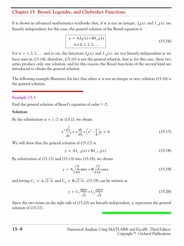
Chapter 15 Bessel, Legendre, and Chebyshev Functions
15−8 Numerical Analysis Using MATLAB® and Excel®, Third EditionCopyright © Orchard Publications
It is shown in advanced mathematics textbooks that, if is not an integer, and arelinearly independent; for this case, the general solution of the Bessel equation is
(15.16)
For and so on, the functions and are not linearly independent as wehave seen in (15.14); therefore, (15.16) is not the general solution, that is, for this case, these twoseries produce only one solution, and for this reason, the Bessel functions of the second kind areintroduced to obtain the general solution.
The following example illustrates the fact that when is not an integer or zero, relation (15.16) isthe general solution.
Example 15.3
Find the general solution of Bessel’s equation of order .
Solution:
By the substitution in (15.1), we obtain
(15.17)
We will show that the general solution of (15.17) is
(15.18)
By substitution of (15.12) and (15.13) into (15.18), we obtain
(15.19)
and letting and , (15.19) can be written as
(15.20)
Since the two terms on the right side of (15.20) are linearly independent, represents the generalsolution of (15.17).
n Jn x( ) J n– x( )
y AJn x( ) BJ n– x( )+=
n 0 1 2 3 …, , , ,≠
n 1 2 3 …, , ,= Jn x( ) J n– x( )
n
1 2⁄
n 1 2⁄=
x2
x2
2
d
d y x xddy x2 1
4---–⎝ ⎠
⎛ ⎞ y+ + 0=
y AJ1 2⁄ x( ) BJ 1 2⁄– x( )+=
y A 2πx------ xsin B 2
πx------ xcos+=
C1 A 2 π⁄= C2 B 2 π⁄=
y C1xsin
x---------- C2
xcosx
-----------+=
y
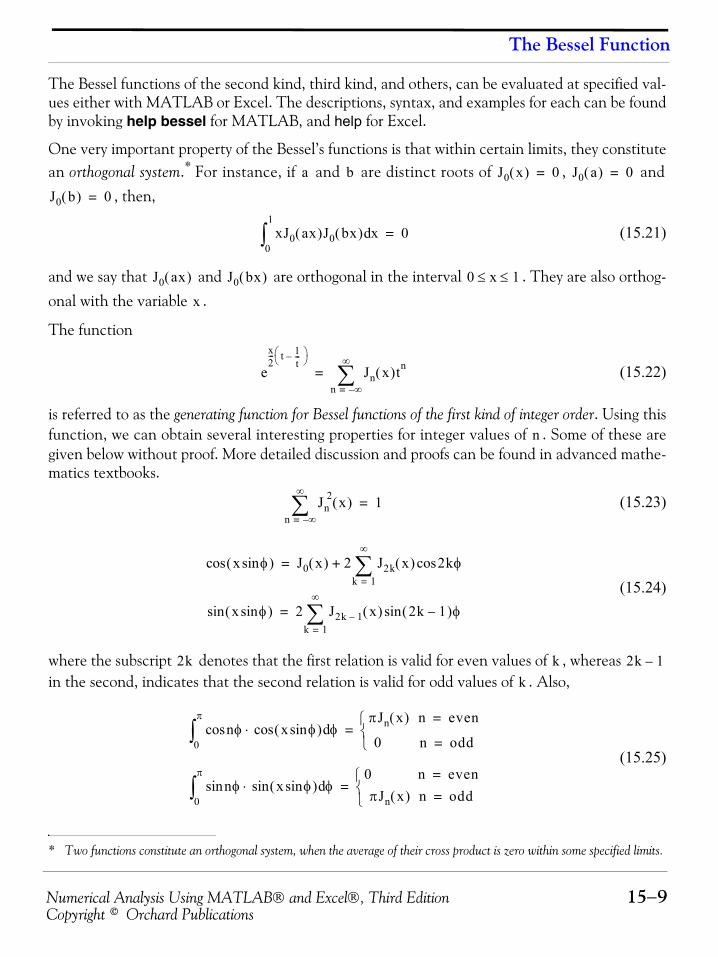
Numerical Analysis Using MATLAB® and Excel®, Third Edition 15−9Copyright © Orchard Publications
The Bessel Function
The Bessel functions of the second kind, third kind, and others, can be evaluated at specified val-ues either with MATLAB or Excel. The descriptions, syntax, and examples for each can be foundby invoking help bessel for MATLAB, and help for Excel.
One very important property of the Bessel’s functions is that within certain limits, they constitutean orthogonal system.* For instance, if and are distinct roots of , and
, then,
(15.21)
and we say that and are orthogonal in the interval . They are also orthog-onal with the variable .
The function
(15.22)
is referred to as the generating function for Bessel functions of the first kind of integer order. Using thisfunction, we can obtain several interesting properties for integer values of . Some of these aregiven below without proof. More detailed discussion and proofs can be found in advanced mathe-matics textbooks.
(15.23)
(15.24)
where the subscript denotes that the first relation is valid for even values of , whereas in the second, indicates that the second relation is valid for odd values of . Also,
(15.25)
* Two functions constitute an orthogonal system, when the average of their cross product is zero within some specified limits.
a b J0 x( ) 0= J0 a( ) 0=
J0 b( ) 0=
xJ0 ax( )J0 bx( ) xd0
1
∫ 0=
J0 ax( ) J0 bx( ) 0 x 1≤ ≤
x
ex2--- t 1
t---–⎝ ⎠
⎛ ⎞
Jn x( )tn
n ∞–=
∞
∑=
n
Jn2 x( )
n ∞–=
∞
∑ 1=
x φsin( )cos J0 x( ) 2 J2k x( ) 2kφcosk 1=
∞
∑+=
x φsin( )sin 2 J2k 1– x( ) 2k 1–( )sin φk 1=
∞
∑=
2k k 2k 1–
k
nφcos x φsin( )cos⋅ φd0
π
∫πJn x( ) n even=
0 n odd=⎩⎨⎧
=
nsin φ x φsin( )sin⋅ φd0
π
∫0 n even=
πJn x( ) n odd=⎩⎨⎧
=
Chapter 15 Bessel, Legendre, and Chebyshev Functions
15−10 Numerical Analysis Using MATLAB® and Excel®, Third EditionCopyright © Orchard Publications
and
(15.26)
Relations (15.23) through (15.26) appear in frequency modulation. For example, the averagepower is shown to be
and with (15.23), it reduces to
15.2 Legendre FunctionsAnother second−order differential equation with variable coefficients is the equation
(15.27)
known as Legendre’s equation. Here, is a constant, and if it is zero or a positive integer, then(15.27) has polynomial solutions of special interest.
Applying the method of Frobenius, as in the Bessel equation, we obtain two independent solu-tions and as follows.
(15.28)
(15.29)
where and are constants. We observe that is an even function of , while is an oddfunction. Then, the general solution of (15.27) is or
(15.30)
and this series is absolutely convergent* for .
Jn x( ) 1π--- nφ x φsin–( ) φdcos
0
π
∫=
Pave12---AC
2 Jn2 β( )
n ∞–=
∞
∑=
Pave12---AC
2=
1 x2–( )d2 y
dx2--------- 2xdy
dx------– n n 1+( )y+ 0=
n
y1 y2
y1 a0 1 n n 1+( )2!
--------------------x2– n 2–( )n n 1+( ) n 3+( )4!
-------------------------------------------------------x4 …–+=
y2 a1 x n 1–( ) n 2+( )3!
----------------------------------x3–n 3–( ) n 1–( ) n 2+( ) n 4+( )
5!---------------------------------------------------------------------x5 …–+=
a0 a1 y1 x y2
y y1 y2+=
y a0 1 n n 1+( )2!
--------------------x2– n 2–( )n n 1+( ) n 3+( )4!
-------------------------------------------------------x4 …–+
a1 x n 1–( ) n 2+( )3!
----------------------------------x3– n 3–( ) n 1–( ) n 2+( ) n 4+( )5!
---------------------------------------------------------------------x5 …–++
=
x 1>
Numerical Analysis Using MATLAB® and Excel®, Third Edition 15−11Copyright © Orchard Publications
Legendre Functions
The parameter is usually a positive integer. If is zero, or an even positive integer, the firstterm on the right side of (15.30) contains only a finite number of terms; if it is odd, the secondterm contains only a finite number of terms. Therefore, whenever is zero or a positive integer;the general solution of Legendre’s equation contains a polynomial solution which is denoted as
, and an infinite series solution which is denoted as .
The Legendre polynomials are defined as
(15.31)
(15.32)
and these are also referred to as surface zonal harmonics. The infinite series solution isreferred to as Legendre functions of the second kind. These become infinite as and theirapplications to science and engineering problems are very limited. Accordingly, they will not bediscussed in this text.
The even and odd functions of (15.31) and (15.32) can be combined to a single relation as
(15.33)
From (15.33), or (15.31) and (15.32), we obtain the following first 6 Legendre polynomials.
* Assume that the infinite series converges, i.e., reaches a limit. If, when we replace the
terms of this series by their absolute value, we find that the resulting series also
converges, this series is said to be absolutely convergent.
un x0( )n 1=
∞
∑ u1 x0( ) u2 x0( ) …+ +=
un x0( )n 1=
∞
∑ u1 x0( ) u2 x0( ) …+ +=
n n
n
Pn x( ) Qn x( )
Pn x( ) 1–( )n 2⁄ 1 3 5 … n 1–( )⋅ ⋅ ⋅ ⋅2 4 6 … n⋅ ⋅ ⋅ ⋅
-------------------------------------------------⋅ 1 n n 1+( )2!
--------------------x2– …+=
for n 0 or n even integer= =
Pn x( ) 1–( ) n 1–( ) 2⁄ 1 3 5 … n⋅ ⋅ ⋅ ⋅2 4 6 … n 1–( )⋅ ⋅ ⋅ ⋅-------------------------------------------------⋅ x n 1–( ) n 2+( )
3!----------------------------------x3– …+=
for n odd integer=
Qn x( )
x 1±→
Pn x( ) 1–( )k 2n 2k–( )!⋅
2nk! n k–( )! n 2k–( )!----------------------------------------------------xn 2k–
k 0=
N
∑=
where N n2--- for n even and N n 1–( )
2---------------- for n odd= = = =
Chapter 15 Bessel, Legendre, and Chebyshev Functions
15−12 Numerical Analysis Using MATLAB® and Excel®, Third EditionCopyright © Orchard Publications
(15.34)
The relation
(15.35)
is known as Rodrigues’ formula, and offers another method of expressing the Legendre polynomials.We prove (15.35) as follows.
From the binomial theorem,
(15.36)
and differentiation of (15.36) with respect to times yields
(15.37)
Now, by comparison with (15.33), we recognize (15.37) as and thus (15.35) isproved.
Another important identity involving Legendre polynomials, is the generating function for Legendrepolynomials which is defined as
(15.38)
We will illustrate the use of the Legendre polynomials with the following example.
Example 15.4
Find the potential difference (voltage) at a point developed by a nearby dipole* in terms ofthe distance between the point and the dipole, and the angle which point makes with thecenter of the dipole.
* A dipole is a pair of electric charges or magnetic poles, of equal magnitude but of opposite sign or polarity, separated by asmall distance. Alternately, a dipole is an antenna, usually fed from the center, consisting of two equal rods extending out-ward in a straight line.
P0 x( ) 1= P1 x( ) x=
P2 x( ) 12--- 3x2 1–( )= P3 x( ) 1
2--- 5x3 3x–( )=
P4 x( ) 18--- 35x4 30x2– 3+( )= P5 x( ) 1
8--- 63x5 70x3– 15x+( )=
Pn x( ) 1
2n n!⋅--------------- d n
dxn--------- x2 1–( )
n⋅=
x2 1–( )n 1–( )k n!⋅
k! n k–( )!⋅----------------------------x2n 2k–
k 0=
n
∑=
x n
d n
dxn-------- x2 1–( )
n 1–( )k n!⋅k! n k–( )!------------------------ 2n 2k–( )!
n 2k–( )!-------------------------⋅ xn 2k–
k 0=
N
∑=
2n n! Pn x( )⋅ ⋅
1
1 2xt– t2+-------------------------------- P0 x( ) P1 x( )t P2 x( )t2 … Pn x( )tn+ + + + Pn x( )tn
n 0=
∞
∑= =
v PP P
Numerical Analysis Using MATLAB® and Excel®, Third Edition 15−13Copyright © Orchard Publications
Legendre Functions
Solution:
Let the charges and of the dipole be a distance 2d apart with the origin 0 as the midpoint asshown in Figure 15.3.
Figure 15.3. Figure for Example 15.4
Let the potential at point be . From electromagnetic field textbooks we find that
(15.39)
where is the permittivity* of the vacuum. For simplicity, we will denote the quantity as k and thus we rewrite (15.39) as
(15.40)
Next, we need to express and in terms or d and r. By the law of cosines,
(15.41)and
(15.42)
Dividing both sides of (15.42) by , we obtain
(15.43)
or
* Permittivity is a measure of the ability of a material to resist the formation of an electric field within it.
q q–
0 q−q d d
r1 r2
r
θ
P
P VP
VPq
4πε0------------ 1
r2---- 1
r1----–⎝ ⎠
⎛ ⎞=
ε0 1 4πε0( )⁄
VP kq 1r2---- 1
r1----–⎝ ⎠
⎛ ⎞ kq r21– r1
1––( )= =
r1 r2
r1 d 2 r2 2– dr 180° θ–( )cos+ d 2 r2 2dr θcos+ += =
r2 d 2 r2 2– dr θcos+=
r
r2r---- d 2
r2------ 1 2d θcos
r------------------–+=
Chapter 15 Bessel, Legendre, and Chebyshev Functions
15−14 Numerical Analysis Using MATLAB® and Excel®, Third EditionCopyright © Orchard Publications
(15.44)
In all practical applications, the point is sufficiently far from the origin; thus, we assume that. Now, we want to relate the terms inside the parentheses of (15.44), to a Legendre polyno-
mial. We do this by expressing these terms in the form of the generating function of (15.38).
We let , and ; then, by substitution into (15.44) we obtain
(15.45)
We recall that (15.45) holds only if and . This requirement is satisfied since x and y,as defined, are both less than unity.
To find a similar expression for , we simply replace with in (15.45), and thus
(15.46)
By substitution of (15.45) and (15.46) into (15.40), we obtain
(15.47)
Since , and , we can express (15.47) as
(15.48)
However, if is even in (15.48), , and therefore, all even powers vanish.But when is odd, and the odd powers in (15.48) are duplicated. Then,
(15.49)
and for , (15.49) can be approximated as
* (15.50)
r21– 1
r--- d 2
r2------ 1 2d θcos
r------------------–+
⎝ ⎠⎜ ⎟⎛ ⎞ 1 2⁄–
=
Pr d>
x θcos= y d r⁄=
d 2
r2----- 1 2d θcos
r------------------–+
⎝ ⎠⎜ ⎟⎛ ⎞ 1 2⁄–
1 2xy– y2+( )1 2⁄–
Pn x( )yn
n 0=
∞
∑= =
x 1< y 1<
r11– x x–
1 2xy y2+ +( )1 2⁄–
Pn x–( )yn
n 0=
∞
∑=
VPkqr
------ Pn x( ) yn Pn x–( )yn–[ ]n 0=
∞
∑=
x θcos= y d r⁄=
VPkqr
------ Pn θcos( ) Pn θcos–( )–[ ]n 0=
∞
∑=dr---⎝ ⎠
⎛ ⎞ n
n Pn θcos–( ) Pn θcos( )=
n Pn θcos–( ) Pn θcos( )–=
VPkqr
------ 2P2n 1+ θcos( )n 0=
∞
∑= dr---⎝ ⎠
⎛ ⎞ 2n 1+
r d»
VP2kq
r---------P1 θcos( ) d
r---⎝ ⎠
⎛ ⎞≈ 2kdqr2
------------- θcos=
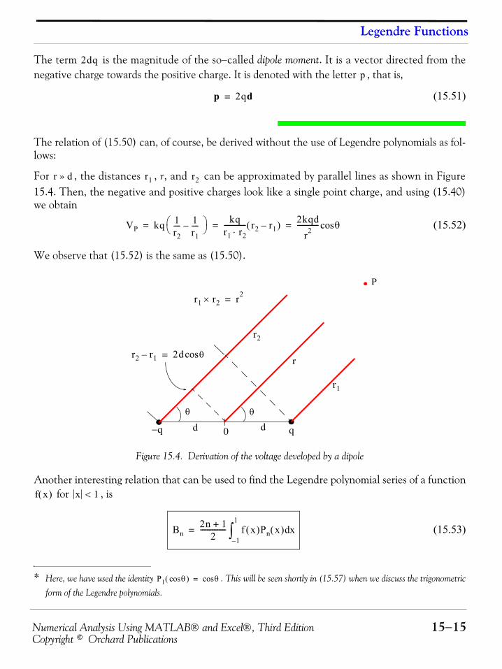
Numerical Analysis Using MATLAB® and Excel®, Third Edition 15−15Copyright © Orchard Publications
Legendre Functions
The term is the magnitude of the so−called dipole moment. It is a vector directed from thenegative charge towards the positive charge. It is denoted with the letter , that is,
(15.51)
The relation of (15.50) can, of course, be derived without the use of Legendre polynomials as fol-lows:
For , the distances , r, and can be approximated by parallel lines as shown in Figure15.4. Then, the negative and positive charges look like a single point charge, and using (15.40)we obtain
(15.52)
We observe that (15.52) is the same as (15.50).
Figure 15.4. Derivation of the voltage developed by a dipole
Another interesting relation that can be used to find the Legendre polynomial series of a function for , is
(15.53)
* Here, we have used the identity . This will be seen shortly in (15.57) when we discuss the trigonometric
form of the Legendre polynomials.
P1 θcos( ) θcos=
2dqp
p 2qd=
r d» r1 r2
VP kq 1r2---- 1
r1----–⎝ ⎠
⎛ ⎞ kqr1 r2⋅------------- r2 r1–( ) 2kqd
r2------------- θcos= = =
0 q−q d d
r
θ
P
θ
r1
r2
r1 r2× r2=
r2 r1– 2d θcos=
f x( ) x 1<
Bn2n 1+
2--------------- f x( )Pn x( ) xd
1–
1
∫=
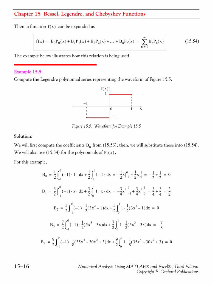
Chapter 15 Bessel, Legendre, and Chebyshev Functions
15−16 Numerical Analysis Using MATLAB® and Excel®, Third EditionCopyright © Orchard Publications
Then, a function can be expanded as
(15.54)
The example below illustrates how this relation is being used.
Example 15.5 Compute the Legendre polynomial series representing the waveform of Figure 15.5.
Figure 15.5. Waveform for Example 15.5
Solution:
We will first compute the coefficients from (15.53); then, we will substitute these into (15.54).We will also use (15.34) for the polynomials of .
For this example,
f x( )
f x( ) B0P0 x( ) B1P1 x( ) B2P2 x( ) … BnPn x( )+ + + + BnPn x( )n 0=
∞
∑= =
−10 1 x
1
−1
f x( )
Bn
Pn x( )
B012--- 1–( ) 1 xd⋅ ⋅
1–
0
∫12--- 1 1 xd⋅ ⋅
0
1
∫+ 12---x 1–
0 12---x 0
1+– 12---– 1
2---+ 0= = = =
B132--- 1–( ) x xd⋅ ⋅
1–
0
∫32--- 1 x xd⋅ ⋅
0
1
∫+34---x2
1–
0 34---x2
0
1+– 3
4--- 3
4---+ 3
2---= = = =
B252--- 1–( ) 1
2--- 3x2 1–( ) xd⋅
1–
0
∫52--- 1 1
2--- 3x2 1–( ) xd⋅
0
1
∫+ 0= =
B372--- 1–( ) 1
2--- 5x3 3x–( ) xd⋅
1–
0
∫72--- 1 1
2--- 5x3 3x–( ) xd⋅
0
1
∫+ 78---–= =
B492--- 1–( ) 1
8--- 35x4 30x2– 3+( ) xd⋅
1–
0
∫92--- 1 1
8--- 35x4 30x2– 3+( )⋅
0
1
∫+ 0= =
Numerical Analysis Using MATLAB® and Excel®, Third Edition 15−17Copyright © Orchard Publications
Legendre Functions
and so on. Therefore, using (15.54) and (15.34) we obtain
(15.55)
We observe that the waveform of is an odd function and, as we found above, its expansioncontains only odd Legendre polynomials.
In many applications, the algebraic form of the Legendre polynomials is usually the most useful.However, there are times when we want to express the polynomials in terms trigonometric func-tions, as we did in Example 15.4. Also, the trigonometric forms are most convenient with thecylindrical and spherical coordinate systems. It is shown in advanced mathematics textbooks that
(15.56)
From (15.56) we obtain the first 6 Legendre polynomials in trigonometric form listed below.
(15.57)
The Legendre polynomials in algebraic form, satisfy the orthogonality principle when asindicated by the following integral.
B511–2
--------- 18--- 63x5 70x3– 15x+( ) xd
1–
0
∫112
------ 18--- 63x5 70x3– 15x+( )
0
1
∫+ 1116------= =
f x( ) 32---P1 x( ) 7
8---P3 x( )– 11
16------P5 x( )+=
32---x 7
8--- 1
2--- 5x3 3x–( ) 11
16------ 1
8--- 63x5 70x3– 15x+( )⋅+⋅–=
32---x 7
16------ 5x3 3x–( ) 11
128--------- 63x5 70x3– 15x+( )⋅+–=
525128---------x 525
64---------x3–
693128---------x5+=
f x( )
Pn θcos 1 3 … 2n 1–( )⋅ ⋅ ⋅2 4 … 2n⋅ ⋅ ⋅
---------------------------------------------2 nθcos 12--- 1 3 … 2n 3–( )⋅ ⋅ ⋅
2 4 … 2n 2–( )⋅ ⋅ ⋅---------------------------------------------⋅ 2 n 2–( )θcos+=
+ 1 3⋅2 4⋅---------- 1 3 … 2n 5–( )⋅ ⋅ ⋅
2 4 … 2n 4–( )⋅ ⋅ ⋅---------------------------------------------2 n 4–( )θcos⋅ …+
P0 θcos 1=
P1 θcos θcos=
P2 θcos 3 2θ 1+cos4
---------------------------=
P3 θcos 5 3θ 3 θcos+cos8
----------------------------------------=
P4 θcos 35 4θ 20 2θ 9+cos+cos64
----------------------------------------------------------=
P5 θcos 63 5θ 35 3θ 30 θcos+cos+cos128
-------------------------------------------------------------------------=
m n≠
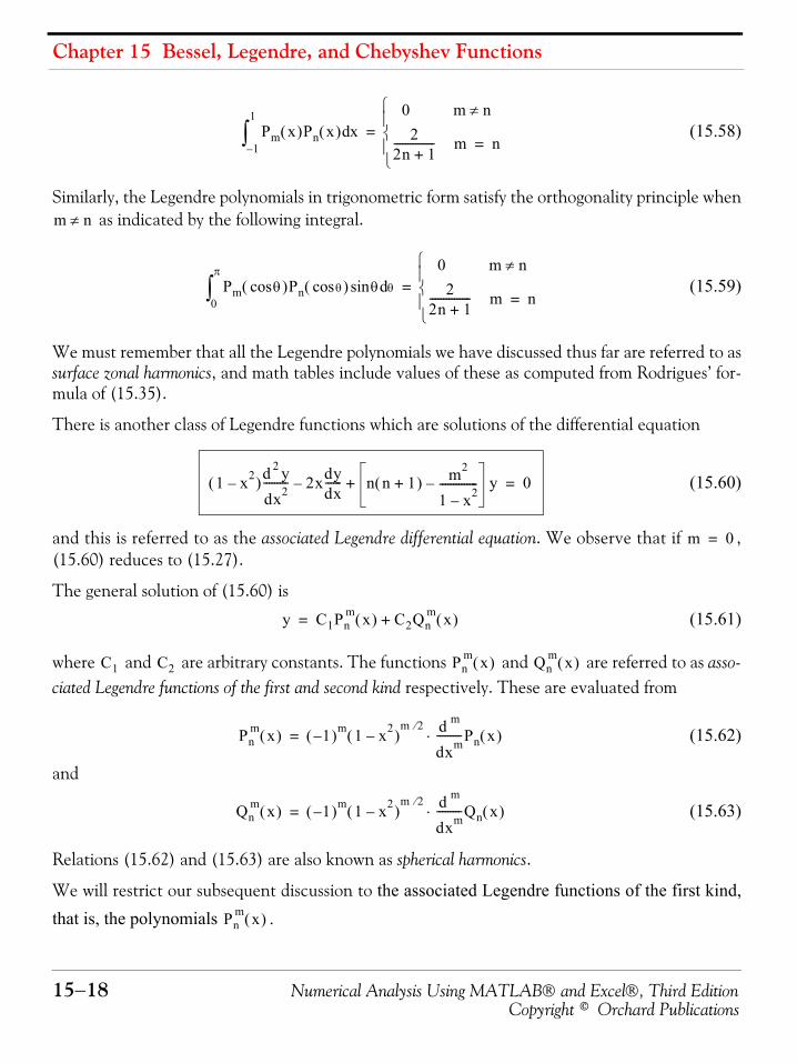
Chapter 15 Bessel, Legendre, and Chebyshev Functions
15−18 Numerical Analysis Using MATLAB® and Excel®, Third EditionCopyright © Orchard Publications
(15.58)
Similarly, the Legendre polynomials in trigonometric form satisfy the orthogonality principle when as indicated by the following integral.
(15.59)
We must remember that all the Legendre polynomials we have discussed thus far are referred to assurface zonal harmonics, and math tables include values of these as computed from Rodrigues’ for-mula of (15.35).
There is another class of Legendre functions which are solutions of the differential equation
(15.60)
and this is referred to as the associated Legendre differential equation. We observe that if ,(15.60) reduces to (15.27).
The general solution of (15.60) is
(15.61)
where and are arbitrary constants. The functions and are referred to as asso-ciated Legendre functions of the first and second kind respectively. These are evaluated from
(15.62)
and
(15.63)
Relations (15.62) and (15.63) are also known as spherical harmonics.
We will restrict our subsequent discussion to the associated Legendre functions of the first kind,that is, the polynomials .
Pm x( )Pn x( ) xd1–
1
∫0 m n≠
22n 1+--------------- m n=
⎩⎪⎨⎪⎧
=
m n≠
Pm θcos( )Pn θcos( ) θsin θd0
π
∫0 m n≠
22n 1+--------------- m n=
⎩⎪⎨⎪⎧
=
1 x2–( )d2 y
dx2--------- 2xdy
dx------– n n 1+( ) m2
1 x2–--------------– y+ 0=
m 0=
y C1Pnm x( ) C2Qn
m x( )+=
C1 C2 Pnm x( ) Qn
m x( )
Pnm x( ) 1–( )m 1 x2–( )
m 2⁄ d m
dxm---------Pn x( )⋅=
Qnm x( ) 1–( )m 1 x2–( )
m 2⁄ d m
dxm---------Qn x( )⋅=
Pnm x( )
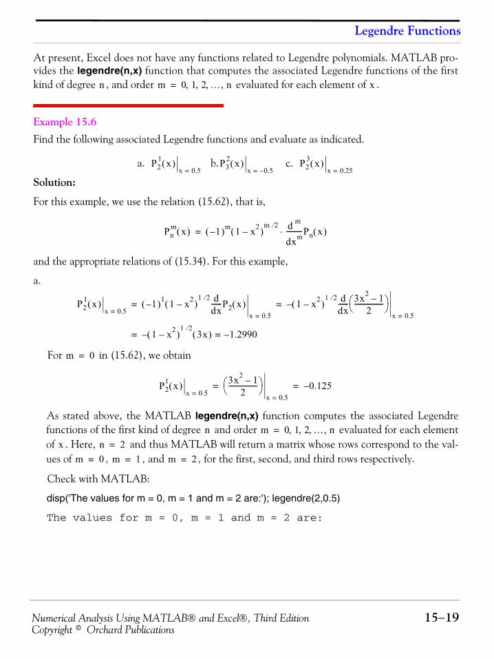
Numerical Analysis Using MATLAB® and Excel®, Third Edition 15−19Copyright © Orchard Publications
Legendre Functions
At present, Excel does not have any functions related to Legendre polynomials. MATLAB pro-vides the legendre(n,x) function that computes the associated Legendre functions of the firstkind of degree , and order evaluated for each element of .
Example 15.6 Find the following associated Legendre functions and evaluate as indicated.
a. b. c.
Solution:
For this example, we use the relation (15.62), that is,
and the appropriate relations of (15.34). For this example,
a.
For in (15.62), we obtain
As stated above, the MATLAB legendre(n,x) function computes the associated Legendrefunctions of the first kind of degree and order evaluated for each elementof . Here, and thus MATLAB will return a matrix whose rows correspond to the val-ues of , , and , for the first, second, and third rows respectively.
Check with MATLAB:
disp('The values for m = 0, m = 1 and m = 2 are:'); legendre(2,0.5)
The values for m = 0, m = 1 and m = 2 are:
n m 0 1 2 … n, , , ,= x
P21 x( )
x 0.5=P3
2 x( )x 0.5–=
P23 x( )
x 0.25=
Pnm x( ) 1–( )m 1 x2–( )
m 2⁄ d m
dxm---------Pn x( )⋅=
P21 x( )
x 0.5=1–( )1 1 x2–( )
1 2⁄ ddx------P2 x( )
x 0.5=
1 x2–( )–1 2⁄ d
dx------ 3x2 1–
2-----------------⎝ ⎠⎛ ⎞
x 0.5=
= =
1 x2–( )–1 2⁄
3x( ) 1.2990–==
m 0=
P21 x( )
x 0.5=
3x2 1–2
-----------------⎝ ⎠⎛ ⎞
x 0.5=
0.125–= =
n m 0 1 2 … n, , , ,=
x n 2=
m 0= m 1= m 2=
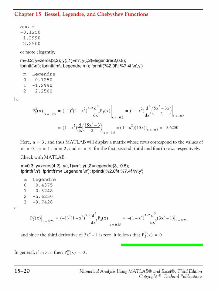
Chapter 15 Bessel, Legendre, and Chebyshev Functions
15−20 Numerical Analysis Using MATLAB® and Excel®, Third EditionCopyright © Orchard Publications
ans =-0.1250-1.2990 2.2500
or more elegantly,
m=0:2; y=zeros(3,2); y(:,1)=m'; y(:,2)=legendre(2,0.5);fprintf('\n'); fprintf('m\t Legendre \n'); fprintf('%2.0f\t %7.4f \n',y')
m Legendre 0 -0.1250 1 -1.2990 2 2.2500
b.
Here, , and thus MATLAB will display a matrix whose rows correspond to the values of, , , and , for the first, second, third and fourth rows respectively.
Check with MATLAB:
m=0:3; y=zeros(4,2); y(:,1)=m'; y(:,2)=legendre(3,−0.5);fprintf('\n'); fprintf('m\t Legendre \n'); fprintf('%2.0f\t %7.4f \n',y')
m Legendre 0 0.4375 1 -0.3248 2 -5.6250 3 -9.7428
c.
and since the third derivative of is zero, it follows that .
In general, if , then .
P32 x( )
x 0.5–=1–( )2 1 x2–( )
2 2⁄ d 2
dx2--------P3 x( )
x 0.5–=
1 x2–( ) d 2
dx2-------- 5x3 3x–
2---------------------⎝ ⎠⎛ ⎞
x 0.5–=
= =
1 x2–( ) ddx------ 15x2 3–
2--------------------⎝ ⎠⎛ ⎞
x 0.5–=
1 x2–( ) 15x( ) x 0.5–=5.6250–= ==
n 3=
m 0= m 1= m 2= m 3=
P23 x( )
x 0.25=1–( )3 1 x2–( )
3 2⁄ d 3
dx3--------P2 x( )
x 0.25=
1 x2–( )–3 2⁄ d 3
dx3-------- 3x2 1–( ) x 0.25=
= =
3x2 1– P23 x( ) 0=
m n> Pnm x( ) 0=
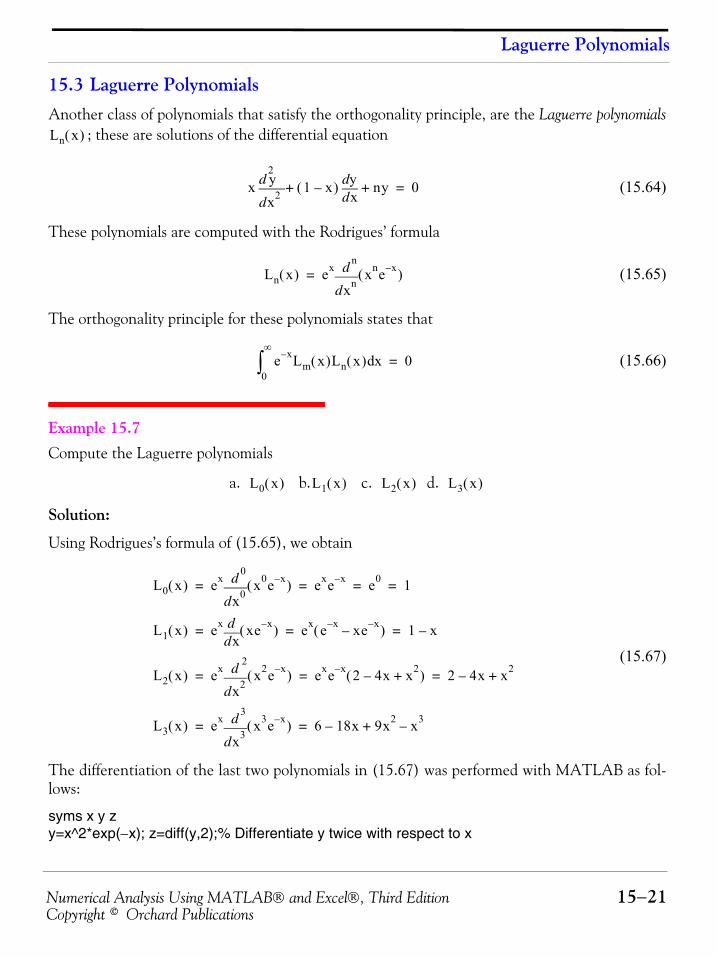
Numerical Analysis Using MATLAB® and Excel®, Third Edition 15−21Copyright © Orchard Publications
Laguerre Polynomials
15.3 Laguerre PolynomialsAnother class of polynomials that satisfy the orthogonality principle, are the Laguerre polynomials
; these are solutions of the differential equation
(15.64)
These polynomials are computed with the Rodrigues’ formula
(15.65)
The orthogonality principle for these polynomials states that
(15.66)
Example 15.7 Compute the Laguerre polynomials
a. b. c. d.
Solution:
Using Rodrigues’s formula of (15.65), we obtain
(15.67)
The differentiation of the last two polynomials in (15.67) was performed with MATLAB as fol-lows:
syms x y zy=x^2*exp(−x); z=diff(y,2);% Differentiate y twice with respect to x
Ln x( )
xx2
2
d
d y 1 x–( ) xddy ny+ + 0=
Ln x( ) ex
xn
n
d
d xne x–( )=
e x– Lm x( )Ln x( ) xd0
∞
∫ 0=
L0 x( ) L1 x( ) L2 x( ) L3 x( )
L0 x( ) ex
x0
0
d
d x0e x–( ) exe x– e0 1= = = =
L1 x( ) ex
xdd xe x–( ) ex e x– xe x––( ) 1 x–= = =
L2 x( ) ex
x2
2
d
d x2e x–( ) exe x– 2 4x– x2+( ) 2 4x– x2+= = =
L3 x( ) ex
x3
3
d
d x3e x–( ) 6 18x– 9x2 x3–+= =
Chapter 15 Bessel, Legendre, and Chebyshev Functions
15−22 Numerical Analysis Using MATLAB® and Excel®, Third EditionCopyright © Orchard Publications
L2x=exp(x)*z; simplify(L2x)
ans =2-4*x+x^2
syms x y z w ; y=x^3*exp(−x); z=diff(y,2);% Differentiate y twice% we cannot differentiate three times at oncew=diff(z);% Differentiate one more timeL3x=exp(x)*w; simplify(L3x)
ans =6-18*x+9*x^2-x^3
15.4 Chebyshev PolynomialsThe Chebyshev polynomials are solutions of the differential equations
(15.68)
and
(15.69)
The solutions of (15.68) are referred to as Chebyshev polynomials of the first kind and are denoted as.* The solutions of (15.69) are the Chebyshev polynomials of the second kind; these are
denoted as . Both kinds comprise a set of orthogonal functions.We will restrict our discussion to the polynomials. We will plot some of these later in thissection.
Two interesting properties of the polynomials are:
1. They exhibit equiripple amplitute characteristics over the range , that is, within thisrange, they oscillate with the same ripple. This property is the basis for the Chebyshev approx-imation in the design of Chebyshev type electric filters.
2. For they increase or decrease more rapidly than any other polynomial of order .
* Some books use the notation for these polynomials. However, another class of orthogonal functions known as
Genenbauer or Ultraspherical functions use the notation and for this reason, we will avoid notation forthe Chebyshev polynomials.
1 x2–( )d2 y
dx2--------- xdy
dx------– n2y+ 0=
1 x2–( )d2 y
dx2--------- 3xdy
dx------– n n 2+( )y+ 0=
y Tn x( )=
Ck x( )
Cna( ) x( ) Ck x( )
y Un x( )=
Tn x( )
Tn x( )
1– x 1≤ ≤
x 1> n
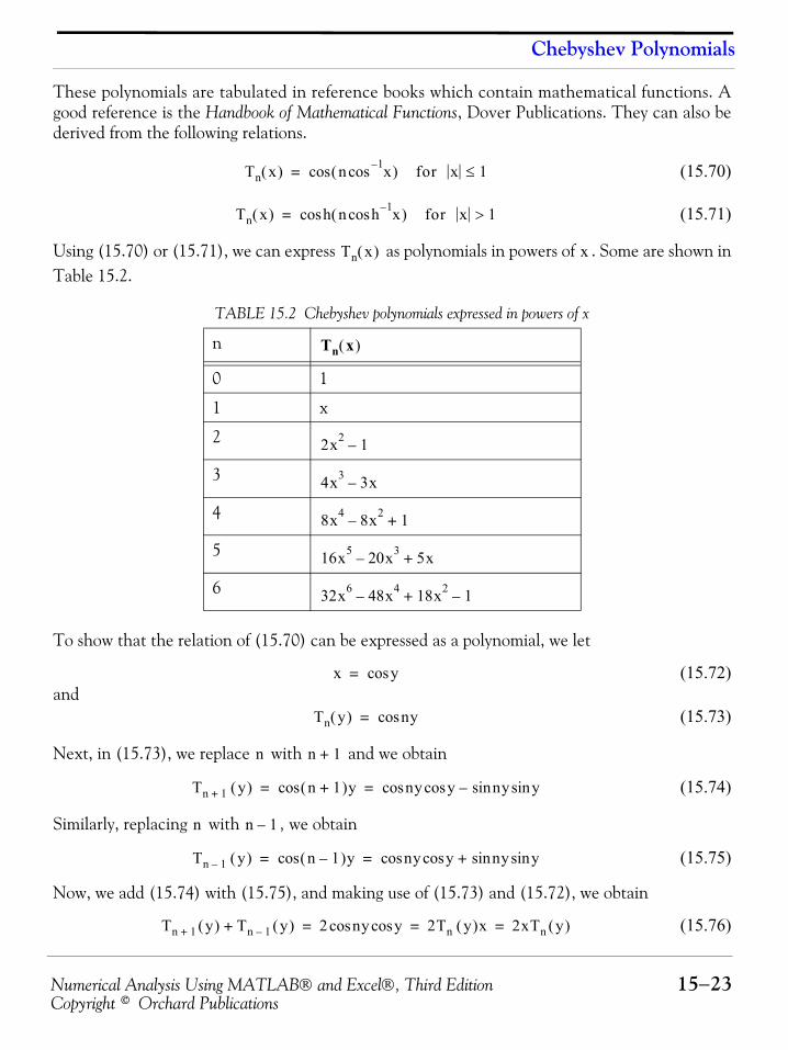
Numerical Analysis Using MATLAB® and Excel®, Third Edition 15−23Copyright © Orchard Publications
Chebyshev Polynomials
These polynomials are tabulated in reference books which contain mathematical functions. Agood reference is the Handbook of Mathematical Functions, Dover Publications. They can also bederived from the following relations.
(15.70)
(15.71)
Using (15.70) or (15.71), we can express as polynomials in powers of . Some are shown inTable 15.2.
To show that the relation of (15.70) can be expressed as a polynomial, we let
(15.72)and
(15.73)
Next, in (15.73), we replace with and we obtain
(15.74)
Similarly, replacing with , we obtain
(15.75)
Now, we add (15.74) with (15.75), and making use of (15.73) and (15.72), we obtain
(15.76)
TABLE 15.2 Chebyshev polynomials expressed in powers of x
n
0 1
1 x
2
3
4
5
6
Tn x( ) n x1–cos( ) for x 1≤cos=
Tn x( ) h n h x1–cos( ) for x 1>cos=
Tn x( ) x
Tn x( )
2x2 1–
4x3 3x–
8x4 8x2– 1+
16x5 20x3– 5x+
32x6 48x4– 18x2 1–+
x ycos=
Tn y( ) nycos=
n n 1+
Tn 1+ y( ) n 1+( )ycos ny ycoscos ny ysinsin–= =
n n 1–
Tn 1– y( ) n 1–( )ycos ny ycoscos ny ysinsin+= =
Tn 1+ y( ) Tn 1– y( )+ 2 ny ycoscos 2Tn y( )x 2xTn y( )= = =
Chapter 15 Bessel, Legendre, and Chebyshev Functions
15−24 Numerical Analysis Using MATLAB® and Excel®, Third EditionCopyright © Orchard Publications
or
Then, we can replace with to obtain
(15.77)
The polynomials in Table 15.2, can now be verified by using a combination of the above relations.Thus, for , (15.73) yields
(15.78)
For , from (15.73) and (15.72), we obtain
(15.79)
To derive the algebraic expressions corresponding to and so on, we use the recurrenceformula of (15.77). For instance, when ,
(15.80)and when ,
(15.81)
Alternately, we can prove the first 3 entries of Table 15.2 with (15.70) by letting .Thus, for ,
For ,
and for ,
or
Relation (15.71) can be derived from (15.70) as follows:
We recall that
Tn 1+ y( ) 2xTn y( ) Tn 1– y( )–=
y x
Tn 1+ x( ) 2xTn x( ) Tn 1– x( )–=
Recurrence Relation
n 0=
T0 y( ) T0 x( ) 1= =
n 1=
T1 y( ) T1 x( ) x= =
n 2 3 4, ,=
n 2=
T2 x( ) 2xT1 x( ) T0 x( )– 2x2 1–= =
n 3=
T3 x( ) 2xT2 x( ) T1 x( )– 4x3 2x– x– 4x3 3x–= = =
y x1–cos=
n 0=
T0 x( ) 0 x1–cos⋅( )cos 0 y⋅( )cos= = 1=
n 1=
T1 x( ) 1 x1–cos⋅( )cos 1 y⋅( )cos ycos= = = x=
n 2=
T2 x( ) 2 x1–cos⋅( )cos 2 y⋅( )cos 2ycos= = 2 y2cos 1–= =
2 x1–cos( )2
cos 1– 2 x1–cos( )cosx
x1–cos( )cosx
⋅ 1–== ⎧ ⎪ ⎪ ⎨ ⎪ ⎪ ⎩ ⎧ ⎪ ⎪ ⎨ ⎪ ⎪ ⎩
T2 x( ) 2x2 1–=
Numerical Analysis Using MATLAB® and Excel®, Third Edition 15−25Copyright © Orchard Publications
Chebyshev Polynomials
(15.82)
and
(15.83)
Then,(15.84)
and when ,* (15.85)
By substitution into (15.70), making use of (15.85), and that , we obtain
and this is the same as (15.71).
We can also use MATLAB to convert (15.70) and (15.71) to polynomials. For example, if ,
syms x; expand(cos(3*acos(x))), expand(cosh(3*acosh(x)))
ans =4*x^3-3*x
ans =4*x^3-3*x
The MATLAB script below plots the for through .
% Chebyshev polynomials%x=−1.2:0.01:1.2; Tnx0=cos(0*acos(x)); Tnx1=cos(1*acos(x)); Tnx2=cos(2*acos(x)); Tnx3=cos(3*acos(x)); Tnx4=cos(4*acos(x)); Tnx5=cos(5*acos(x)); Tnx6=cos(6*acos(x));plot(x, Tnx0, x, Tnx1, x, Tnx2, x, Tnx3, x, Tnx4, x, Tnx5, x, Tnx6);....axis([−1.2 1.2 −1.5 1.5]); grid; title('Chebyshev Polynomials of the First Kind');xlabel('x'); ylabel('Tn(x)')% We could have used the gtext function to label the curves but it is easier with the Figure text % tool
* Let ; then , , and (15.85) follows.
αcos e jα e j– α+2
------------------------=
hαcos eα e α–+2
--------------------=
αcos hjαcos=
x 1>
x1–cos j x1–cosh–=
αcos jαcosh v= = α v1–cos= jα v1–cosh= j v1–cos v1–cosh=
t–( )cosh tcosh=
Tn x( ) n j x1–cosh–( )[ ]cos jn x1–cosh–( )cos jnj x1–cosh( )cosh= = =
j jn x1–cosh–( )[ ]cosh= n x1–cosh( )cosh=
n 3=
Tn x( ) n 0= n 6=
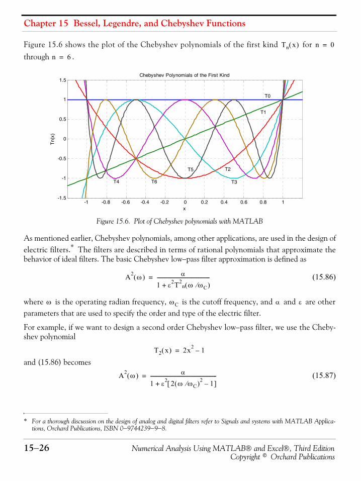
Chapter 15 Bessel, Legendre, and Chebyshev Functions
15−26 Numerical Analysis Using MATLAB® and Excel®, Third EditionCopyright © Orchard Publications
Figure 15.6 shows the plot of the Chebyshev polynomials of the first kind for through .
Figure 15.6. Plot of Chebyshev polynomials with MATLAB
As mentioned earlier, Chebyshev polynomials, among other applications, are used in the design ofelectric filters.* The filters are described in terms of rational polynomials that approximate thebehavior of ideal filters. The basic Chebyshev low−pass filter approximation is defined as
(15.86)
where is the operating radian frequency, is the cutoff frequency, and and are otherparameters that are used to specify the order and type of the electric filter.
For example, if we want to design a second order Chebyshev low−pass filter, we use the Cheby-shev polynomial
and (15.86) becomes
(15.87)
* For a thorough discussion on the design of analog and digital filters refer to Signals and systems with MATLAB Applica-tions, Orchard Publications, ISBN 0−9744239−9−8.
Tn x( ) n 0=
n 6=
-1 -0.8 -0.6 -0.4 -0.2 0 0.2 0.4 0.6 0.8 1-1.5
-1
-0.5
0
0.5
1
1.5Chebyshev Polynomials of the First Kind
x
Tn(
x)
T0
T1
T2
T3T4 T6
T5
A2 ω( ) α
1 ε2T2n ω ωC⁄( )+
-------------------------------------------=
ω ωC α ε
T2 x( ) 2x2 1–=
A2 ω( ) α
1 ε2 2 ω ωC⁄( )2 1–[ ]+------------------------------------------------------=
Numerical Analysis Using MATLAB® and Excel®, Third Edition 15−27Copyright © Orchard Publications
Summary
15.5 Summary• Differential equations with variable coefficients cannot be solved in terms of familiar functions
as those which we encountered in ordinary differential equations with constant coefficients.The usual procedure is to derive solutions in the form of infinite series, and the most commonare the Method of Frobenius and the Method of Picard.
• Bessel functions are solutions of the differential equation
where can be any number, positive or negative integer, fractional, or even a complex num-ber. The general solution depends on the value of .
• The series
where is any positive real number or zero is referred to as Bessel function of order .
• The series
is referred to as the Bessel function of negative order .
• For and the series reduce to
• Two more useful relations are
x2
x2
2
d
d y x xddy x2 n2–( )y+ + 0=
nn
Jn x( ) 1–( )k
k 0=
∞
∑x2---⎝ ⎠
⎛ ⎞ n 2k+ 1k! Γ n k 1+ +( )⋅----------------------------------------⋅ ⋅ n 0≥=
n n
J n– x( ) 1–( )k
k 0=
∞
∑x2---⎝ ⎠
⎛ ⎞ n– 2k+ 1k! Γ n– k 1+ +( )⋅--------------------------------------------⋅ ⋅ =
n
n 0 1,= 2
J0 x( ) 1 x2
22 1!( )2⋅----------------------– x4
24 2!( )2⋅---------------------- x6
26 3!( )2⋅---------------------- x8
28 4!( )2⋅---------------------- …–+–+=
J1 x( ) x2--- x3
23 1! 2!⋅ ⋅------------------------– x5
25 2! 3!⋅ ⋅------------------------ x7
27 3! 4!⋅ ⋅------------------------ x9
29 4! 5!⋅ ⋅------------------------ …–+–+=
J2 x( ) x2
22 2!⋅-------------- x4
24 1! 3!⋅ ⋅------------------------– x6
26 2! 4!⋅ ⋅------------------------ x8
28 3! 5!⋅ ⋅------------------------ x10
210 4! 6!⋅ ⋅-------------------------- …–+–+=
xdd J0 x( ) J1 x( )–=
Chapter 15 Bessel, Legendre, and Chebyshev Functions
15−28 Numerical Analysis Using MATLAB® and Excel®, Third EditionCopyright © Orchard Publications
• Values of can be calculated using the appropriate series given above. They also can befound in math table books, and can also be found with the MATLAB besselj(n,x) function orthe Excel BESSELJ(x,n) function.
• The Bessel functions
and
are known as half−order Bessel functions.
• Besides the above functions known as Bessel functions of the first kind, other Bessel functions,denoted as and referred to as Bessel functions of the second kind, or Weber functions,or Neumann functions exist. Also, certain differential equations resemble the Bessel equation,and thus their solutions are called Modified Bessel functions, or Hankel functions.
• If is not an integer, and are linearly independent; for this case, the general solu-tion of the Bessel equation is
• If and are distinct roots of , and , then,
and thus we say that and are orthogonal in the interval .
• The differential equation
where is a constant, is known as Legendre’s equation.
• The infinite series solution of the Legendre functions, denoted as , is referred to as Leg-endre functions of the second kind.
xdd xJ1 x( ){ } xJ0 x( )=
Jn x( )
J1 2⁄ x( ) 2πx------ xsin= J 1 2⁄–( ) x( ) 2
πx------ xcos=
Yn x( )
n Jn x( ) J n– x( )
y AJn x( ) BJ n– x( )+=
n 0 1 2 3 …, , , ,≠
a b J0 x( ) 0= J0 a( ) 0= J0 b( ) 0=
xJ0 ax( )J0 bx( ) xd0
1
∫ 0=
J0 ax( ) J0 bx( ) 0 x 1≤ ≤
1 x2–( )d2 y
dx2--------- 2xdy
dx------– n n 1+( )y+ 0=
n
Qn x( )
Numerical Analysis Using MATLAB® and Excel®, Third Edition 15−29Copyright © Orchard Publications
Summary
• The Legendre polynomials are defined as
and the first 6 Legendre polynomials are
• The relation
is known as Rodrigues’ formula, and offers another method of expressing the Legendre polyno-mials.
• The Legendre polynomial series of a function for , is
and with this relation we can find a polynomial defined as
• The trigonometric form of the Legendre polynomials is
and the first 6 Legendre polynomials in trigonometric form listed below.
Pn x( ) 1–( )k 2n 2k–( )!⋅
2nk! n k–( )! n 2k–( )!----------------------------------------------------xn 2k–
k 0=
N
∑=
where N n2--- for n even and N n 1–( )
2---------------- for n odd= = = =
P0 x( ) 1= P1 x( ) x=
P2 x( ) 12--- 3x2 1–( )= P3 x( ) 1
2--- 5x3 3x–( )=
P4 x( ) 18--- 35x4 30x2– 3+( )= P5 x( ) 1
8--- 63x5 70x3– 15x+( )=
Pn x( ) 1
2n n!⋅--------------- d n
dxn--------- x2 1–( )
n⋅=
f x( ) x 1<
Bn2n 1+
2--------------- f x( )Pn x( ) xd
1–
1
∫=
f x( )
f x( ) B0P0 x( ) B1P1 x( ) B2P2 x( ) … BnPn x( )+ + + + BnPn x( )n 0=
∞
∑= =
Pn θcos 1 3 … 2n 1–( )⋅ ⋅ ⋅2 4 … 2n⋅ ⋅ ⋅
---------------------------------------------2 nθcos 12--- 1 3 … 2n 3–( )⋅ ⋅ ⋅
2 4 … 2n 2–( )⋅ ⋅ ⋅---------------------------------------------⋅ 2 n 2–( )θcos+=
+ 1 3⋅2 4⋅---------- 1 3 … 2n 5–( )⋅ ⋅ ⋅
2 4 … 2n 4–( )⋅ ⋅ ⋅---------------------------------------------2 n 4–( )θcos⋅ …+
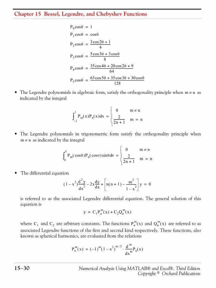
Chapter 15 Bessel, Legendre, and Chebyshev Functions
15−30 Numerical Analysis Using MATLAB® and Excel®, Third EditionCopyright © Orchard Publications
• The Legendre polynomials in algebraic form, satisfy the orthogonality principle when asindicated by the integral
• The Legendre polynomials in trigonometric form satisfy the orthogonality principle when as indicated by the integral
• The differential equation
is referred to as the associated Legendre differential equation. The general solution of thisequation is
where and are arbitrary constants. The functions and are referred to asassociated Legendre functions of the first and second kind respectively. These functions, alsoknown as spherical harmonics, are evaluated from the relations
P0 θcos 1=
P1 θcos θcos=
P2 θcos 3 2θ 1+cos4
---------------------------=
P3 θcos 5 3θ 3 θcos+cos8
----------------------------------------=
P4 θcos 35 4θ 20 2θ 9+cos+cos64
----------------------------------------------------------=
P5 θcos 63 5θ 35 3θ 30 θcos+cos+cos128
-------------------------------------------------------------------------=
m n≠
Pm x( )Pn x( ) xd1–
1
∫0 m n≠
22n 1+--------------- m n=
⎩⎪⎨⎪⎧
=
m n≠
Pm θcos( )Pn θcos( ) θsin θd0
π
∫0 m n≠
22n 1+--------------- m n=
⎩⎪⎨⎪⎧
=
1 x2–( )d2 y
dx2--------- 2xdy
dx------– n n 1+( ) m2
1 x2–--------------– y+ 0=
y C1Pnm x( ) C2Qn
m x( )+=
C1 C2 Pnm x( ) Qn
m x( )
Pnm x( ) 1–( )m 1 x2–( )
m 2⁄ d m
dxm---------Pn x( )⋅=
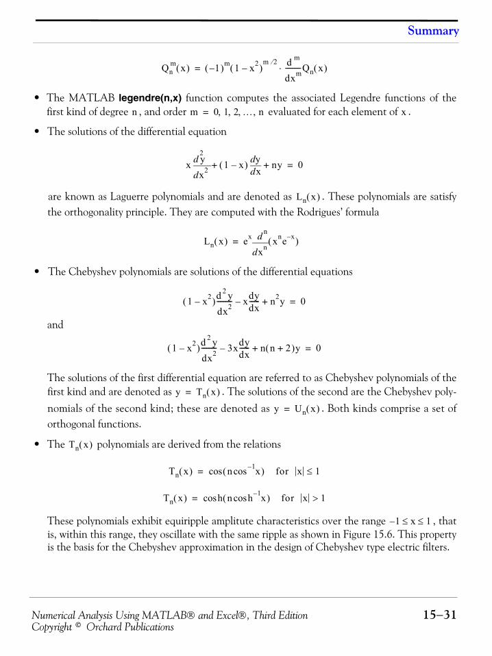
Numerical Analysis Using MATLAB® and Excel®, Third Edition 15−31Copyright © Orchard Publications
Summary
• The MATLAB legendre(n,x) function computes the associated Legendre functions of thefirst kind of degree , and order evaluated for each element of .
• The solutions of the differential equation
are known as Laguerre polynomials and are denoted as . These polynomials are satisfythe orthogonality principle. They are computed with the Rodrigues’ formula
• The Chebyshev polynomials are solutions of the differential equations
and
The solutions of the first differential equation are referred to as Chebyshev polynomials of thefirst kind and are denoted as . The solutions of the second are the Chebyshev poly-nomials of the second kind; these are denoted as . Both kinds comprise a set oforthogonal functions.
• The polynomials are derived from the relations
These polynomials exhibit equiripple amplitute characteristics over the range , thatis, within this range, they oscillate with the same ripple as shown in Figure 15.6. This propertyis the basis for the Chebyshev approximation in the design of Chebyshev type electric filters.
Qnm x( ) 1–( )m 1 x2–( )
m 2⁄ d m
dxm---------Qn x( )⋅=
n m 0 1 2 … n, , , ,= x
xx2
2
d
d y 1 x–( ) xddy ny+ + 0=
Ln x( )
Ln x( ) ex
xn
n
d
d xne x–( )=
1 x2–( )d2 y
dx2--------- xdy
dx------– n2y+ 0=
1 x2–( )d2 y
dx2--------- 3xdy
dx------– n n 2+( )y+ 0=
y Tn x( )=
y Un x( )=
Tn x( )
Tn x( ) n x1–cos( ) for x 1≤cos=
Tn x( ) h n h x1–cos( ) for x 1>cos=
1– x 1≤ ≤
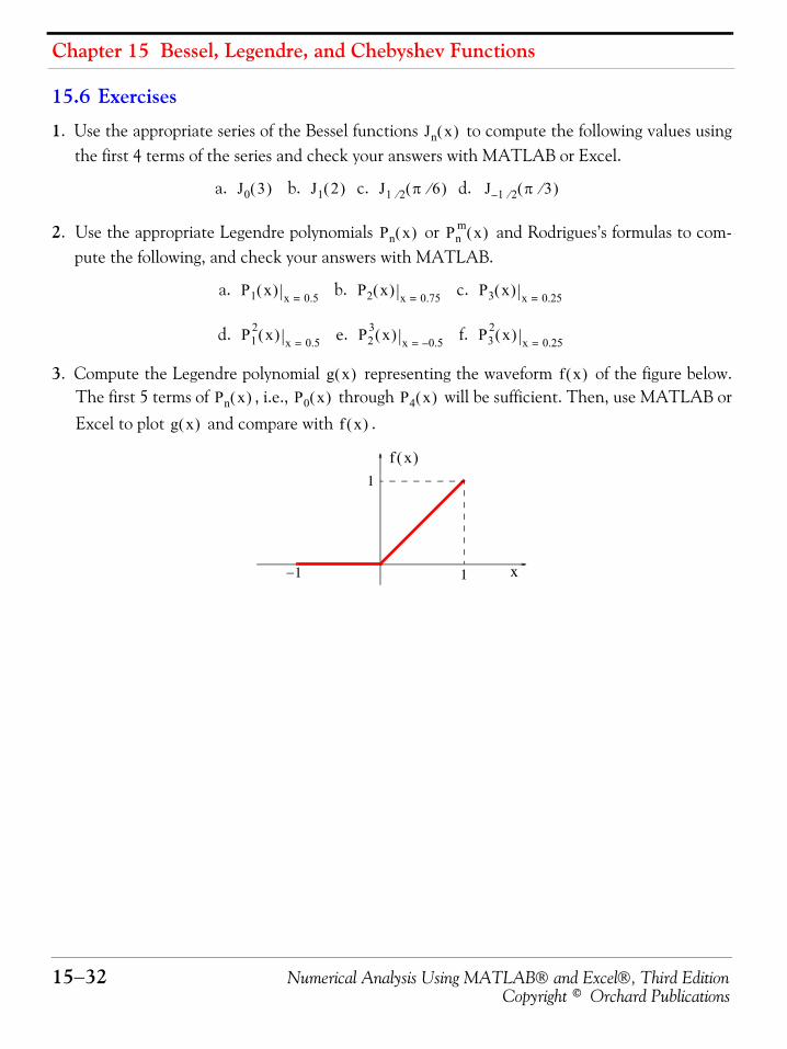
Chapter 15 Bessel, Legendre, and Chebyshev Functions
15−32 Numerical Analysis Using MATLAB® and Excel®, Third EditionCopyright © Orchard Publications
15.6 Exercises
1. Use the appropriate series of the Bessel functions to compute the following values usingthe first 4 terms of the series and check your answers with MATLAB or Excel.
a. b. c. d.
2. Use the appropriate Legendre polynomials or and Rodrigues’s formulas to com-pute the following, and check your answers with MATLAB.
a. b. c.
d. e. f.
3. Compute the Legendre polynomial representing the waveform of the figure below.The first 5 terms of , i.e., through will be sufficient. Then, use MATLAB orExcel to plot and compare with .
Jn x( )
J0 3( ) J1 2( ) J1 2⁄ π 6⁄( ) J 1– 2⁄ π 3⁄( )
Pn x( ) Pnm x( )
P1 x( ) x 0.5=P2 x( ) x 0.75=
P3 x( ) x 0.25=
P12 x( ) x 0.5=
P23 x( ) x 0.5–=
P32 x( ) x 0.25=
g x( ) f x( )Pn x( ) P0 x( ) P4 x( )
g x( ) f x( )
x1−1
1
f x( )
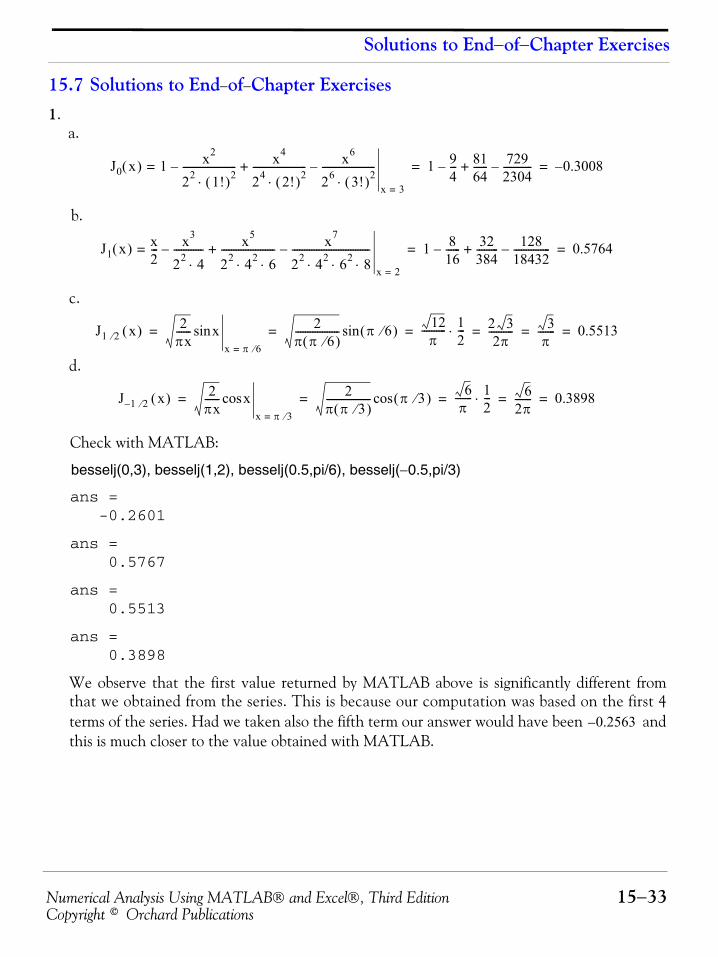
Numerical Analysis Using MATLAB® and Excel®, Third Edition 15−33Copyright © Orchard Publications
Solutions to End−of−Chapter Exercises
15.7 Solutions to End−of−Chapter Exercises1.
a.
b.
c.
d.
Check with MATLAB:
besselj(0,3), besselj(1,2), besselj(0.5,pi/6), besselj(−0.5,pi/3)
ans = -0.2601
ans = 0.5767
ans = 0.5513
ans = 0.3898
We observe that the first value returned by MATLAB above is significantly different fromthat we obtained from the series. This is because our computation was based on the first 4terms of the series. Had we taken also the fifth term our answer would have been andthis is much closer to the value obtained with MATLAB.
J0 x( ) 1 x2
22 1!( )2⋅----------------------– x4
24 2!( )2⋅---------------------- x6
26 3!( )2⋅----------------------–+=
x 3=
1 94---– 81
64------ 729
2304------------–+ 0.3008–= =
J1 x( ) x2--- x3
22 4⋅------------– x5
22 42 6⋅ ⋅---------------------- x7
22 42 62 8⋅ ⋅ ⋅--------------------------------–+=
x 2=
1 816------– 32
384--------- 128
18432---------------–+ 0.5764= =
J1 2⁄ x( ) 2πx------ xsin
x π 6⁄=
2π π 6⁄( )------------------ π 6⁄( )sin 12
π---------- 1
2---⋅ 2 3
2π---------- 3
π------- 0.5513= = = = = =
J 1– 2⁄ x( ) 2πx------ xcos
x π 3⁄=
2π π 3⁄( )------------------ π 3⁄( )cos 6
π------- 1
2---⋅ 6
2π------- 0.3898= = = = =
0.2563–
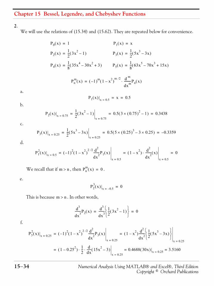
Chapter 15 Bessel, Legendre, and Chebyshev Functions
15−34 Numerical Analysis Using MATLAB® and Excel®, Third EditionCopyright © Orchard Publications
2.We will use the relations of (15.34) and (15.62). They are repeated below for convenience.
a.
b.
c.
d.
We recall that if , then .
e.
This is because . In other words,
f.
P0 x( ) 1= P1 x( ) x=
P2 x( ) 12--- 3x2 1–( )= P3 x( ) 1
2--- 5x3 3x–( )=
P4 x( ) 18--- 35x4 30x2– 3+( )= P5 x( ) 1
8--- 63x5 70x3– 15x+( )=
Pnm x( ) 1–( )m 1 x2–( )
m 2⁄ d m
dxm---------Pn x( )⋅=
P1 x( ) x 0.5=x 0.5= =
P2 x( ) x 0.75=12--- 3x2 1–( )
x 0.75=
0.5 3 0.75( )2× 1–( ) 0.3438= = =
P3 x( ) x 0.25=12--- 5x3 3x–( )
x 0.25=
0.5 5 0.25( )3× 3 0.25×–( ) 0.3359–= = =
P12 x( ) x 0.5=
1–( )2 1 x2–( )2 2⁄ d2
dx2--------P1 x( )
x 0.5=
1 x2–( ) d2
dx2-------- x( )⋅
x 0.5=
0= = =
m n> Pnm x( ) 0=
P23 x( ) x 0.5–=
0=
m n>
d3
dx3--------P2 x( ) d3
dx3-------- 1
2--- 3x2 1–( )
⎩ ⎭⎨ ⎬⎧ ⎫
0= =
P32 x( ) x 0.25=
1–( )2 1 x2–( )2 2⁄ d2
dx2--------P3 x( )
x 0.25=
1 x2–( ) d2
dx2-------- 1
2--- 5x3 3x–( )
⎩ ⎭⎨ ⎬⎧ ⎫
x 0.25=
= =
1 0.252–( ) 12--- d
dx------ 15x2 3–( )⋅ ⋅
x 0.25=
0.4688 30x( ) x 0.25=3.5160= ==
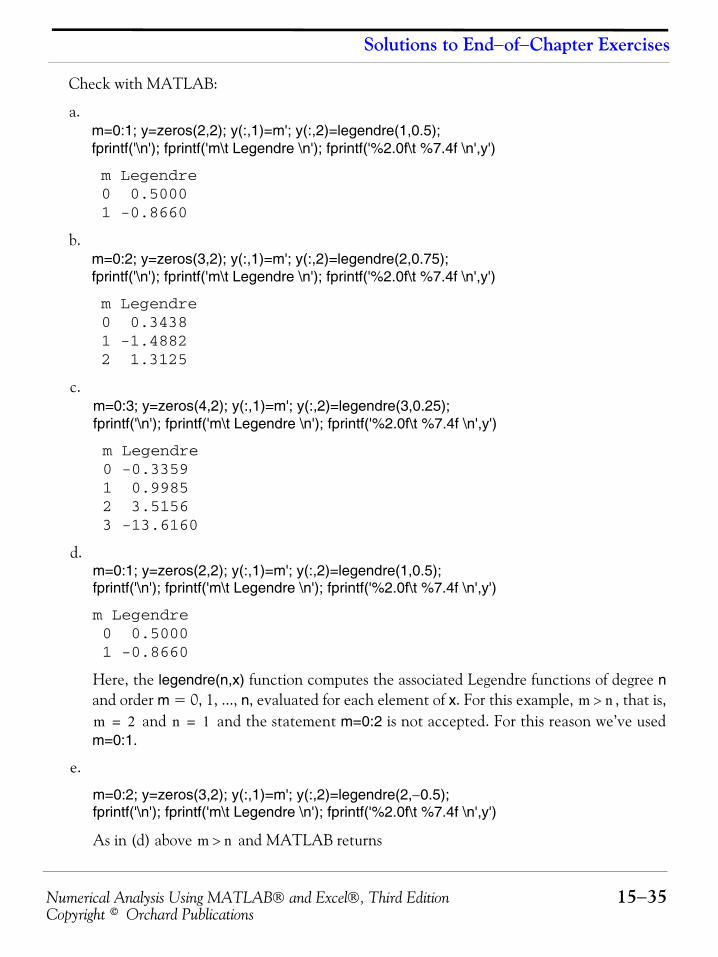
Numerical Analysis Using MATLAB® and Excel®, Third Edition 15−35Copyright © Orchard Publications
Solutions to End−of−Chapter Exercises
Check with MATLAB:
a.m=0:1; y=zeros(2,2); y(:,1)=m'; y(:,2)=legendre(1,0.5);fprintf('\n'); fprintf('m\t Legendre \n'); fprintf('%2.0f\t %7.4f \n',y')
m Legendre 0 0.5000 1 -0.8660
b.m=0:2; y=zeros(3,2); y(:,1)=m'; y(:,2)=legendre(2,0.75);fprintf('\n'); fprintf('m\t Legendre \n'); fprintf('%2.0f\t %7.4f \n',y')
m Legendre 0 0.3438 1 -1.4882 2 1.3125
c.m=0:3; y=zeros(4,2); y(:,1)=m'; y(:,2)=legendre(3,0.25);fprintf('\n'); fprintf('m\t Legendre \n'); fprintf('%2.0f\t %7.4f \n',y')
m Legendre 0 -0.3359 1 0.9985 2 3.5156 3 -13.6160
d.m=0:1; y=zeros(2,2); y(:,1)=m'; y(:,2)=legendre(1,0.5);fprintf('\n'); fprintf('m\t Legendre \n'); fprintf('%2.0f\t %7.4f \n',y')
m Legendre 0 0.5000 1 -0.8660
Here, the legendre(n,x) function computes the associated Legendre functions of degree nand order m = 0, 1, ..., n, evaluated for each element of x. For this example, , that is,
and and the statement m=0:2 is not accepted. For this reason we’ve usedm=0:1.
e.
m=0:2; y=zeros(3,2); y(:,1)=m'; y(:,2)=legendre(2,−0.5);fprintf('\n'); fprintf('m\t Legendre \n'); fprintf('%2.0f\t %7.4f \n',y')
As in (d) above and MATLAB returns
m n>m 2= n 1=
m n>
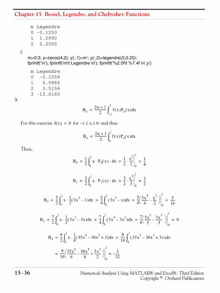
Chapter 15 Bessel, Legendre, and Chebyshev Functions
15−36 Numerical Analysis Using MATLAB® and Excel®, Third EditionCopyright © Orchard Publications
m Legendre 0 -0.1250 1 1.2990 2 2.2500
f.m=0:3; y=zeros(4,2); y(:,1)=m'; y(:,2)=legendre(3,0.25);fprintf('\n'); fprintf('m\t Legendre \n'); fprintf('%2.0f\t %7.4f \n',y')
m Legendre 0 -0.3359 1 0.9985 2 3.5156 3 -13.6160
3.
For this exercise for and thus
Then,
Bn2n 1+
2--------------- f x( )Pn x( ) xd
1–
1
∫=
f x( ) 0= 1 x 0≤ ≤–
Bn2n 1+
2--------------- f x( )Pn x( ) xd
0
1
∫=
B012--- x P0 x( ) xd⋅ ⋅
0
1
∫12--- x2
2-----⋅
0
114---= = =
B132--- x P1 x( ) xd⋅ ⋅
0
1
∫32--- x3
3-----⋅
0
112---= = =
B252--- x 1
2--- 3x2 1–( ) xd⋅
0
1
∫54--- 3x3 x–( ) xd
0
1
∫54--- 3x4
4-------- x2
2-----–⎝ ⎠
⎛ ⎞0
15
16------= = = =
B372--- x 1
2--- 5x3 3x–( ) xd⋅
0
1
∫74--- 5x4 3x2–( ) xd
0
1
∫74--- 5x5
5-------- 3x3
3--------–⎝ ⎠
⎛ ⎞0
1
0= = = =
B492--- x 1
8--- 35x4 30x2– 3+( )⋅ xd
0
1
∫916------ 35x5 30x3– 3x+( ) xd
0
1
∫= =
916------ 35x6
6----------- 30x4
4-----------– 3x2
2--------+⎝ ⎠
⎛ ⎞0
13
32------–==
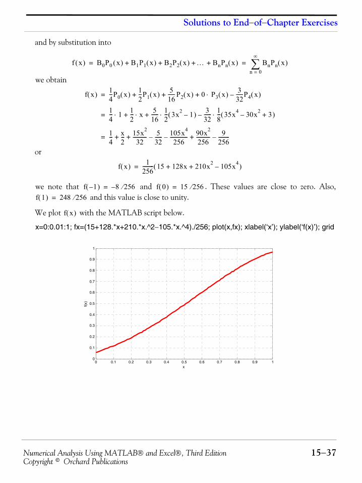
Numerical Analysis Using MATLAB® and Excel®, Third Edition 15−37Copyright © Orchard Publications
Solutions to End−of−Chapter Exercises
and by substitution into
we obtain
or
we note that and . These values are close to zero. Also, and this value is close to unity.
We plot with the MATLAB script below.
x=0:0.01:1; fx=(15+128.*x+210.*x.^2−105.*x.^4)./256; plot(x,fx); xlabel(‘x’); ylabel(‘f(x)’); grid
f x( ) B0P0 x( ) B1P1 x( ) B2P2 x( ) … BnPn x( )+ + + + BnPn x( )n 0=
∞
∑= =
f x( ) 14---P0 x( ) 1
2---P1 x( ) 5
16------ P2 x( ) 0 P3 x( )⋅ 3
32------P4 x( )–+ + +=
14--- 1⋅ 1
2--- x⋅ 5
16------ 1
2--- 3x2 1–( )⋅ 3
32------ 1
8--- 35x4 30x2– 3+( )⋅–+ +=
14--- x
2--- 15x2
32----------- 5
32------– 105x4
256--------------– 90x2
256----------- 9
256---------–+ + +=
f x( ) 1256--------- 15 128x 210x2 105x4–+ +( )=
f 1–( ) 8 256⁄–= f 0( ) 15 256⁄=
f 1( ) 248 256⁄=
f x( )
0 0.1 0.2 0.3 0.4 0.5 0.6 0.7 0.8 0.9 10
0.1
0.2
0.3
0.4
0.5
0.6
0.7
0.8
0.9
1
x
f(x)
Numerical Analysis Using MATLAB® and Excel®, Third Edition 16−1Copyright © Orchard Publications
Chapter 16
Optimization Methods
his chapter introduces three methods for maximizing or minimizing some function in orderto achieve the optimum solution. These methods are topics discussed in detail in a branch ofmathematics called operations research and it is concerned with financial and engineering
economic problems. Our intent here is to introduce these methods with the basic ideas. We willdiscuss linear programming, dynamic programming, and network analysis, and we will illustratethese with some simple but practical examples.
16.1 Linear Programming
In linear* programming we seek to maximize or minimize a particular quantity, referred to as theobjective, which is dependent on a finite number of variables. These variables may or may not beindependent of each another, and in most cases are subject to certain conditions or limitationsreferred to as constraints.
Example 16.1
The ABC Semiconductor Corporation produces microprocessors ( ) and memory ( )chips. The material types, and , required to manufacture the and and the profitsfor each are shown in Table 16.1.
Due to limited supplies of silicon, phosphorus and boron, its product mix at times of high con-sumer demand, is subject to limited supplies. Thus, ABC Semiconductor can only buy parts ofMaterial , and parts of Material . This corporation needs to know what combination of
and will maximize the overall profit.
* A linear program is one in which the variables form a linear combination,i.e., are linearly related. All other programs areconsidered non−linear.
TABLE 16.1 Data for Example 16.1
Parts of Material Types
(1000s)
Semiconductor Material 3 2
Semiconductor Material 5 10
Profit $25.00 per unit $20.00 per 1000
T
μPs RAMA B μPs RAMs
μPs RAMs
A
B
450A 1000 B
μPs RAMs
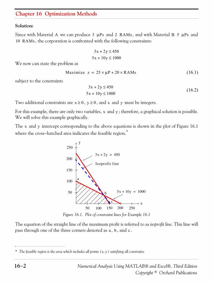
Chapter 16 Optimization Methods
16−2 Numerical Analysis Using MATLAB® and Excel®, Third EditionCopyright © Orchard Publications
Solution:
Since with Material we can produce and , and with Material and , the corporation is confronted with the following constraints:
We now can state the problem as
(16.1)
subject to the constraints
(16.2)
Two additional constraints are , , and and must be integers.
For this example, there are only two variables, and ; therefore, a graphical solution is possible.We will solve this example graphically.
The and intercept corresponding to the above equations is shown in the plot of Figure 16.1where the cross−hatched area indicates the feasible region.*
Figure 16.1. Plot of constraint lines for Example 16.1
The equation of the straight line of the maximum profit is referred to as isoprofit line. This line willpass through one of the three corners denoted as , , and .
* The feasible region is the area which includes all points ( ) satisfying all constrains.
A 3 μPs 2 RAMs B 5 μPs10 RAMs
3x 2y+ 450≤5x 10y+ 1000≤
Maximize z 25 μP 20 RAMs×+×=
3x 2y+ 450≤5x 10y+ 1000≤
x 0≥ y 0≥ x y
x y
x y
x y,
50
100
10050
150
200
250
150 200 250
3x 2y+ 450=
5x 10y+ 1000=
Isoprofit line
x
y
a
b
c
a b c
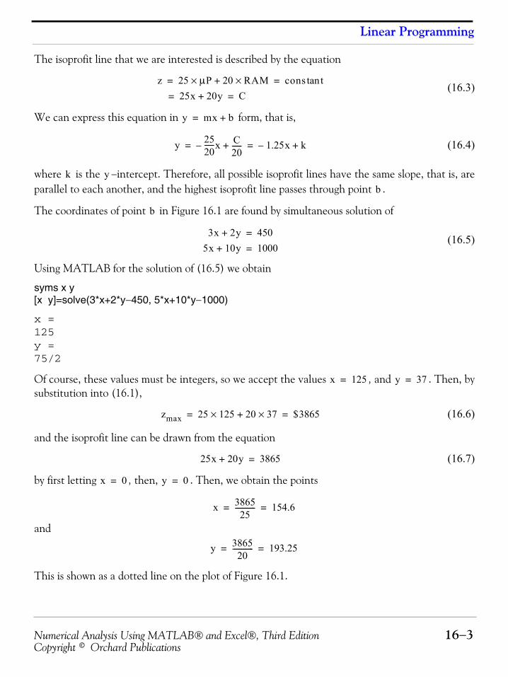
Numerical Analysis Using MATLAB® and Excel®, Third Edition 16−3Copyright © Orchard Publications
Linear Programming
The isoprofit line that we are interested is described by the equation
(16.3)
We can express this equation in form, that is,
(16.4)
where is the −intercept. Therefore, all possible isoprofit lines have the same slope, that is, areparallel to each another, and the highest isoprofit line passes through point .
The coordinates of point in Figure 16.1 are found by simultaneous solution of
(16.5)
Using MATLAB for the solution of (16.5) we obtain
syms x y[x y]=solve(3*x+2*y−450, 5*x+10*y−1000)
x =125y =75/2
Of course, these values must be integers, so we accept the values , and . Then, bysubstitution into (16.1),
(16.6)
and the isoprofit line can be drawn from the equation
(16.7)
by first letting , then, . Then, we obtain the points
and
This is shown as a dotted line on the plot of Figure 16.1.
z 25 μP 20 RAM×+× cons ttan= =
25x 20y+= C=
y mx b+=
y 2520------x– C
20------+ 1.25x– k+= =
k yb
b
3x 2y+ 450=
5x 10y+ 1000=
x 125= y 37=
zmax 25 125 20 37×+× $3865= =
25x 20y+ 3865=
x 0= y 0=
x 386525
------------ 154.6= =
y 386520
------------ 193.25= =
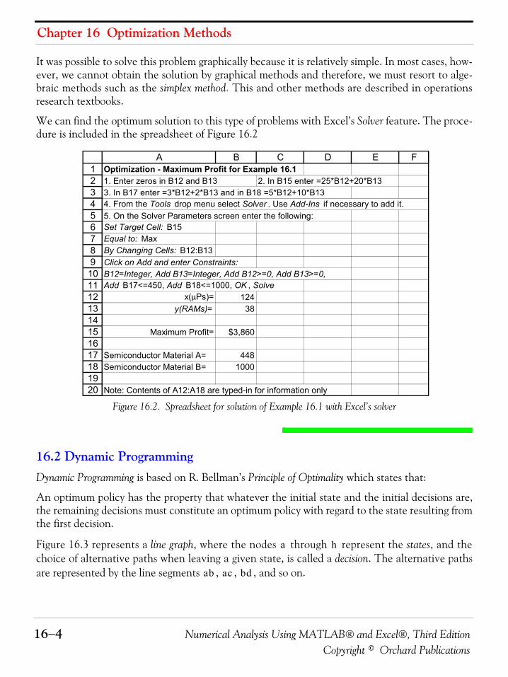
Chapter 16 Optimization Methods
16−4 Numerical Analysis Using MATLAB® and Excel®, Third EditionCopyright © Orchard Publications
It was possible to solve this problem graphically because it is relatively simple. In most cases, how-ever, we cannot obtain the solution by graphical methods and therefore, we must resort to alge-braic methods such as the simplex method. This and other methods are described in operationsresearch textbooks.
We can find the optimum solution to this type of problems with Excel’s Solver feature. The proce-dure is included in the spreadsheet of Figure 16.2
Figure 16.2. Spreadsheet for solution of Example 16.1 with Excel’s solver
16.2 Dynamic ProgrammingDynamic Programming is based on R. Bellman’s Principle of Optimality which states that:
An optimum policy has the property that whatever the initial state and the initial decisions are,the remaining decisions must constitute an optimum policy with regard to the state resulting fromthe first decision.
Figure 16.3 represents a line graph, where the nodes through represent the states, and thechoice of alternative paths when leaving a given state, is called a decision. The alternative pathsare represented by the line segments , , , and so on.
1234567891011121314151617181920
A B C D E FOptimization - Maximum Profit for Example 16.11. Enter zeros in B12 and B13 2. In B15 enter =25*B12+20*B133. In B17 enter =3*B12+2*B13 and in B18 =5*B12+10*B134. From the Tools drop menu select Solver . Use Add-Ins if necessary to add it.5. On the Solver Parameters screen enter the following:Set Target Cell: B15Equal to: MaxBy Changing Cells: B12:B13Click on Add and enter Constraints:B12=Integer, Add B13=Integer, Add B12>=0, Add B13>=0,Add B17<=450, Add B18<=1000, OK , Solve
x(μPs)= 124y(RAMs)= 38
Maximum Profit= $3,860
Semiconductor Material A= 448Semiconductor Material B= 1000
Note: Contents of A12:A18 are typed-in for information only
a h
ab ac bd
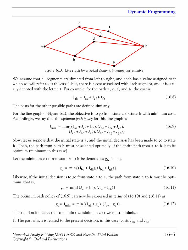
Numerical Analysis Using MATLAB® and Excel®, Third Edition 16−5Copyright © Orchard Publications
Dynamic Programming
Figure 16.3. Line graph for a typical dynamic programming example
We assume that all segments are directed from left to right, and each has a value assigned to itwhich we will refer to as the cost. Thus, there is a cost associated with each segment, and it is usu-ally denoted with the letter . For example, for the path , , , and , the cost is
(16.8)
The costs for the other possible paths are defined similarly.
For the line graph of Figure 16.3, the objective is to go from state to state with minimum cost.Accordingly, we say that the optimum path policy for this line graph is
(16.9)
Now, let us suppose that the initial state is , and the initial decision has been made to go to state. Then, the path from to must be selected optimally, if the entire path from to is to be
optimum (minimum in this case).
Let the minimum cost from state to be denoted as . Then,
(16.10)
Likewise, if the initial decision is to go from state to , the path from state to must be opti-mum, that is,
(16.11)
The optimum path policy of (16.9) can now be expressed in terms of (16.10) and (16.11) as
(16.12)
This relation indicates that to obtain the minimum cost we must minimize:
1. The part which is related to the present decision, in this case, costs and .
a
b
c
d
f
g
h
e
J a c f h
Jah Jac Jcf Jfh+ +=
a h
Jmin min Jac Jcf Jfh+ +( ) Jac Jce Jeh+ +( )Jab Jbd Jdh+ +( ) Jab Jbg Jgh+ +( )
, ,,
{}
=
ab b h a h
b h gb
gb min Jbd Jdh+( ) Jbg Jgh+( ),{ }=
a c c h
gc min Jcf Jfh+( ) Jce Jeh+( ),{ }=
ga Jmin= min Jab gb+( ) Jac gc+( ),{ }=
Jab Jac
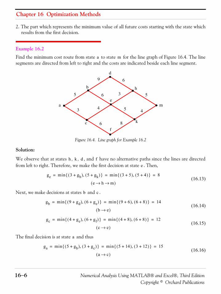
Chapter 16 Optimization Methods
16−6 Numerical Analysis Using MATLAB® and Excel®, Third EditionCopyright © Orchard Publications
2. The part which represents the minimum value of all future costs starting with the state whichresults from the first decision.
Example 16.2
Find the minimum cost route from state to state for the line graph of Figure 16.4. The linesegments are directed from left to right and the costs are indicated beside each line segment.
Figure 16.4. Line graph for Example 16.2
Solution:
We observe that at states , , , and have no alternative paths since the lines are directedfrom left to right. Therefore, we make the first decision at state . Then,
(16.13)
Next, we make decisions at states and .
(16.14)
(16.15)
The final decision is at state and thus
(16.16)
a m
k
h
f
d
e
c
b
ma
5
6
3
4
6
3
69
8
4
5
5
h k d fe
ge min 3 gh+( ) 5 gk+( ),{ } min 3 5+( ) 5 4+( ),{ } 8= = =
e h m→ →( )
b c
gb min 9 gd+( ) 6 ge+( ),{ } min 9 6+( ) 6 8+( ),{ } 14= = =
b e→( )
gc min 4 ge+( ) 6 gf+( ),{ } min 4 8+( ) 6 8+( ),{ } 12= = =
c e→( )
a
ga min 5 gb+( ) 3 gc+( ),{ } min 5 14+( ) 3 12+( ),{ } 15= = =
a c→( )
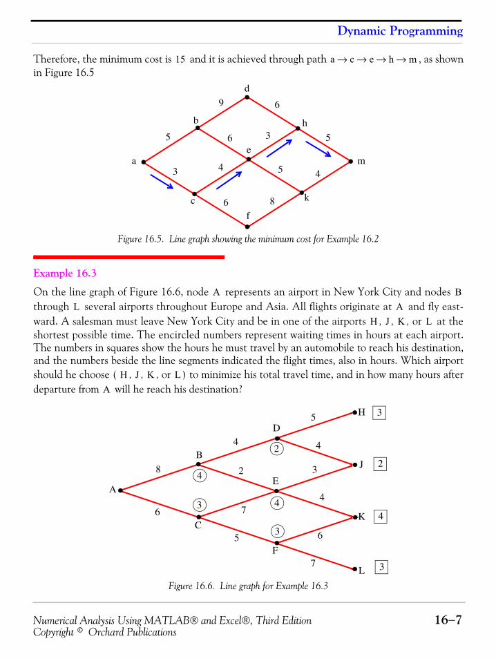
Numerical Analysis Using MATLAB® and Excel®, Third Edition 16−7Copyright © Orchard Publications
Dynamic Programming
Therefore, the minimum cost is and it is achieved through path , as shownin Figure 16.5
Figure 16.5. Line graph showing the minimum cost for Example 16.2
Example 16.3
On the line graph of Figure 16.6, node represents an airport in New York City and nodes through several airports throughout Europe and Asia. All flights originate at and fly east-ward. A salesman must leave New York City and be in one of the airports , , , or at theshortest possible time. The encircled numbers represent waiting times in hours at each airport.The numbers in squares show the hours he must travel by an automobile to reach his destination,and the numbers beside the line segments indicated the flight times, also in hours. Which airportshould he choose ( , , , or ) to minimize his total travel time, and in how many hours afterdeparture from will he reach his destination?
Figure 16.6. Line graph for Example 16.3
15 a c e h m→ → → →
k
h
f
d
e
c
b
ma
5
6
3
4
6
3
69
8
4
5
5
A BL A
H J K L
H J K LA
A
B
D
H
C
F
L
E
J
K 4
2
3
3
4
2
3 4
3
8
6
5
7
4
5
4
3
4
6
2
7
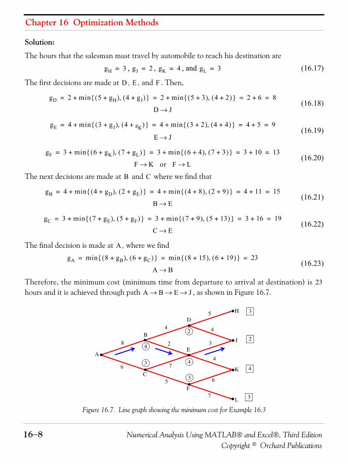
Chapter 16 Optimization Methods
16−8 Numerical Analysis Using MATLAB® and Excel®, Third EditionCopyright © Orchard Publications
Solution:
The hours that the salesman must travel by automobile to reach his destination are
, , , and (16.17)
The first decisions are made at , , and . Then,
(16.18)
(16.19)
(16.20)
The next decisions are made at and where we find that
(16.21)
(16.22)
The final decision is made at , where we find
(16.23)
Therefore, the minimum cost (minimum time from departure to arrival at destination) is hours and it is achieved through path , as shown in Figure 16.7.
Figure 16.7. Line graph showing the minimum cost for Example 16.3
gH 3= gJ 2= gK 4= gL 3=
D E F
gD 2 min 5 gH+( ) 4 gJ+( ),{ }+ 2 min 5 3+( ) 4 2+( ),{ }+ 2 6+ 8= = = =
D J→
gE 4 min 3 gJ+( ) 4 gK+( ),{ }+ 4 min 3 2+( ) 4 4+( ),{ }+ 4 5+ 9= = = =
E J→
gF 3 min 6 gK+( ) 7 gL+( ),{ }+ 3 min 6 4+( ) 7 3+( ),{ }+ 3 10+ 13= = = =
F K or F L→→
B C
gB 4 min 4 gD+( ) 2 gE+( ),{ }+ 4 min 4 8+( ) 2 9+( ),{ }+ 4 11+ 15= = = =
B E→
gC 3 min 7 gE+( ) 5 gF+( ),{ }+ 3 min 7 9+( ) 5 13+( ),{ }+ 3 16+ 19= = = =
C E→
A
gA min 8 gB+( ) 6 gC+( ),{ } min 8 15+( ) 6 19+( ),{ } 23= = =
A B→
23A B E J→ → →
A
B
D
H
C
F
L
E
J
K 4
2
3
3
4
2
3 4
3
8
6
5
7
4
5
4
3
4
6
2
7
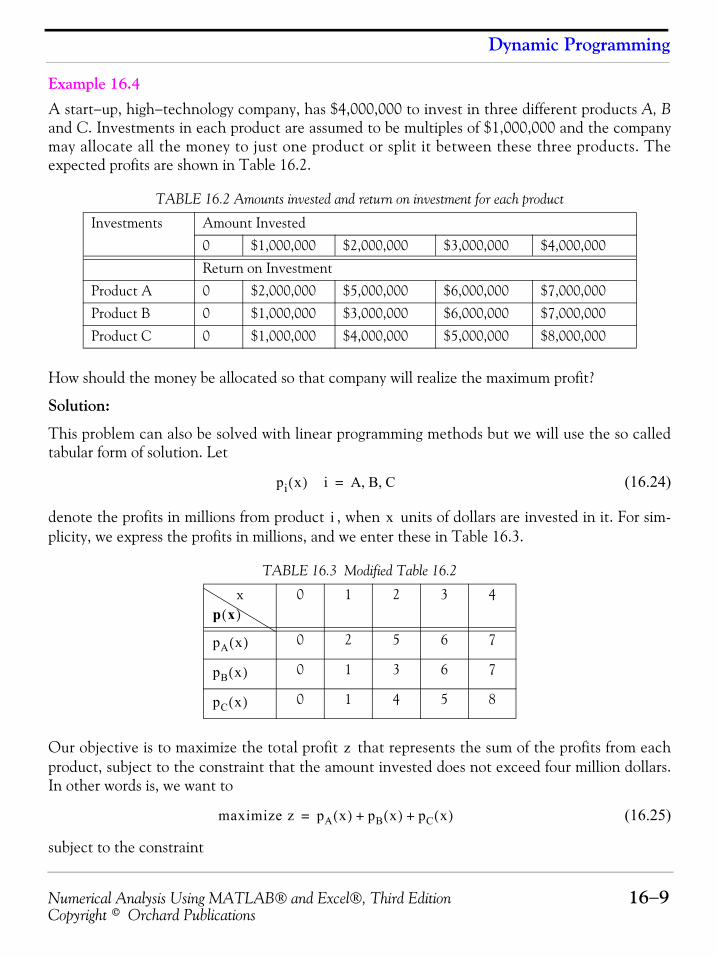
Numerical Analysis Using MATLAB® and Excel®, Third Edition 16−9Copyright © Orchard Publications
Dynamic Programming
Example 16.4 A start−up, high−technology company, has $4,000,000 to invest in three different products A, Band C. Investments in each product are assumed to be multiples of $1,000,000 and the companymay allocate all the money to just one product or split it between these three products. Theexpected profits are shown in Table 16.2.
How should the money be allocated so that company will realize the maximum profit?
Solution:
This problem can also be solved with linear programming methods but we will use the so calledtabular form of solution. Let
(16.24)
denote the profits in millions from product , when units of dollars are invested in it. For sim-plicity, we express the profits in millions, and we enter these in Table 16.3.
Our objective is to maximize the total profit that represents the sum of the profits from eachproduct, subject to the constraint that the amount invested does not exceed four million dollars.In other words is, we want to
(16.25)
subject to the constraint
TABLE 16.2 Amounts invested and return on investment for each product
Investments Amount Invested
0 $1,000,000 $2,000,000 $3,000,000 $4,000,000
Return on Investment
Product A 0 $2,000,000 $5,000,000 $6,000,000 $7,000,000
Product B 0 $1,000,000 $3,000,000 $6,000,000 $7,000,000
Product C 0 $1,000,000 $4,000,000 $5,000,000 $8,000,000
TABLE 16.3 Modified Table 16.2
x 0 1 2 3 4
0 2 5 6 7
0 1 3 6 7
0 1 4 5 8
pi x( ) i A B C, ,=
i x
p x( )
pA x( )
pB x( )
pC x( )
z
maximize z pA x( ) pB x( ) pC x( )+ +=
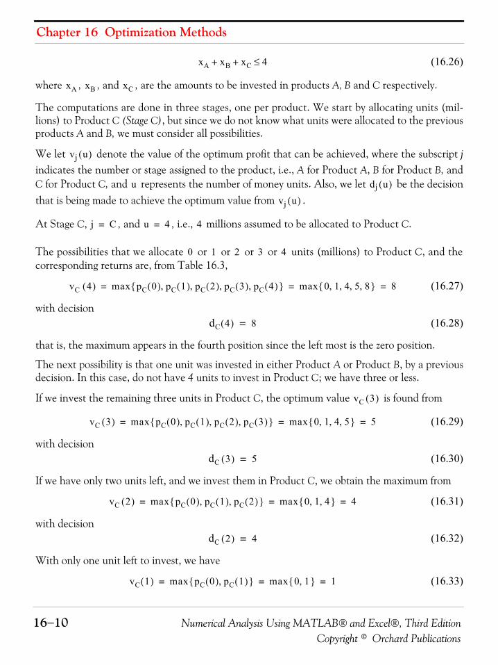
Chapter 16 Optimization Methods
16−10 Numerical Analysis Using MATLAB® and Excel®, Third EditionCopyright © Orchard Publications
(16.26)
where , , and , are the amounts to be invested in products A, B and C respectively.
The computations are done in three stages, one per product. We start by allocating units (mil-lions) to Product C (Stage C), but since we do not know what units were allocated to the previousproducts A and B, we must consider all possibilities.
We let denote the value of the optimum profit that can be achieved, where the subscript jindicates the number or stage assigned to the product, i.e., A for Product A, B for Product B, andC for Product C, and represents the number of money units. Also, we let be the decisionthat is being made to achieve the optimum value from .
At Stage C, , and , i.e., millions assumed to be allocated to Product C.
The possibilities that we allocate or or or or units (millions) to Product C, and thecorresponding returns are, from Table 16.3,
(16.27)
with decision(16.28)
that is, the maximum appears in the fourth position since the left most is the zero position.
The next possibility is that one unit was invested in either Product A or Product B, by a previousdecision. In this case, do not have 4 units to invest in Product C; we have three or less.
If we invest the remaining three units in Product C, the optimum value is found from
(16.29)
with decision(16.30)
If we have only two units left, and we invest them in Product C, we obtain the maximum from
(16.31)
with decision(16.32)
With only one unit left to invest, we have
(16.33)
xA xB xC+ + 4≤
xA xB xC
vj u( )
u dj u( )vj u( )
j C= u 4= 4
0 1 2 3 4
vC 4( ) max pC 0( ) pC 1( ) pC 2( ) pC 3( ) pC 4( ),,,,{ } max 0 1 4 5 8, , , ,{ } 8= = =
dC 4( ) 8=
vC 3( )
vC 3( ) max pC 0( ) pC 1( ) pC 2( ) pC 3( ),,,{ } max 0 1 4 5, , ,{ } 5= = =
dC 3( ) 5=
vC 2( ) max pC 0( ) pC 1( ) pC 2( ),,{ } max 0 1 4, ,{ } 4= = =
dC 2( ) 4=
vC 1( ) max pC 0( ) pC 1( ),{ } max 0 1,{ } 1= = =
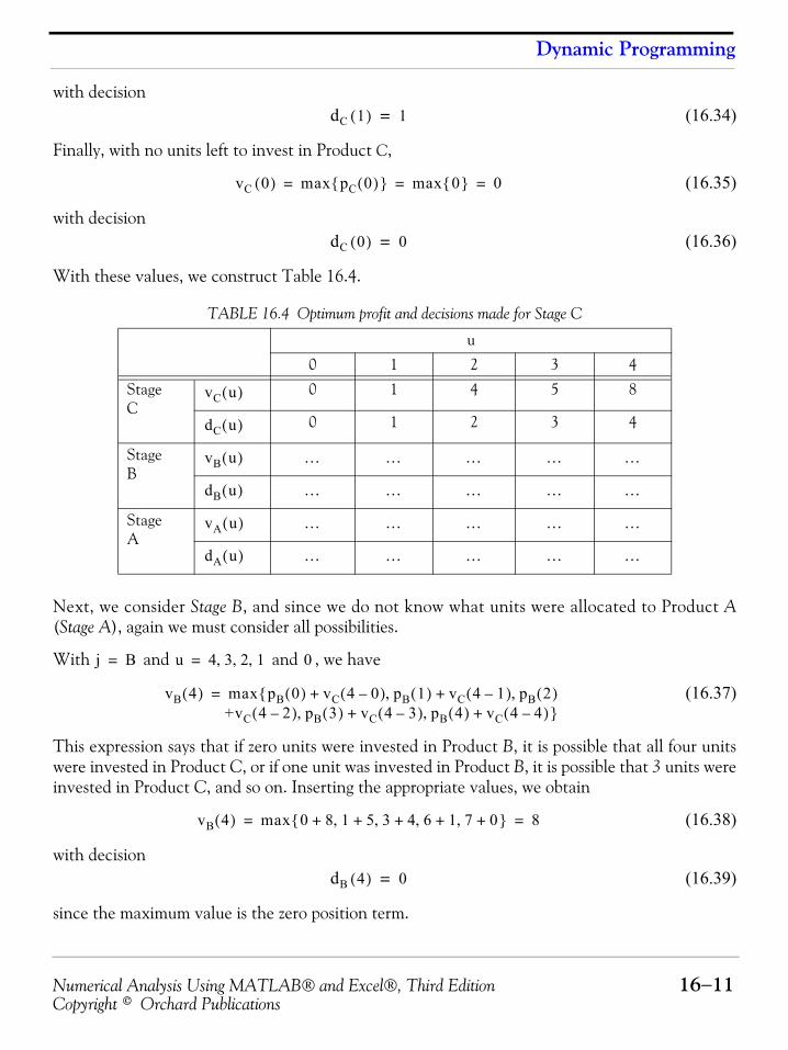
Numerical Analysis Using MATLAB® and Excel®, Third Edition 16−11Copyright © Orchard Publications
Dynamic Programming
with decision(16.34)
Finally, with no units left to invest in Product C,
(16.35)
with decision(16.36)
With these values, we construct Table 16.4.
Next, we consider Stage B, and since we do not know what units were allocated to Product A(Stage A), again we must consider all possibilities.
With and and , we have
(16.37)
This expression says that if zero units were invested in Product B, it is possible that all four unitswere invested in Product C, or if one unit was invested in Product B, it is possible that 3 units wereinvested in Product C, and so on. Inserting the appropriate values, we obtain
(16.38)
with decision(16.39)
since the maximum value is the zero position term.
TABLE 16.4 Optimum profit and decisions made for Stage C
u
0 1 2 3 4
StageC
0 1 4 5 8
0 1 2 3 4
StageB
StageA
dC 1( ) 1=
vC 0( ) max pC 0( ){ } max 0{ } 0= = =
dC 0( ) 0=
vC u( )
dC u( )
vB u( ) … … … … …
dB u( ) … … … … …
vA u( ) … … … … …
dA u( ) … … … … …
j B= u 4 3 2 1, , ,= 0
vB 4( ) max pB 0( ) vC 4 0–( )+ pB 1( ) vC 4 1–( ) pB 2( )+vC 4 2–( ) pB 3( ) vC 4 3–( ) pB 4( ) vC 4 4–( )+,+,
,+,{}
=
vB 4( ) max 0 8 1 5 3 4 6 1 7 0+,+,+,+,+{ } 8= =
dB 4( ) 0=
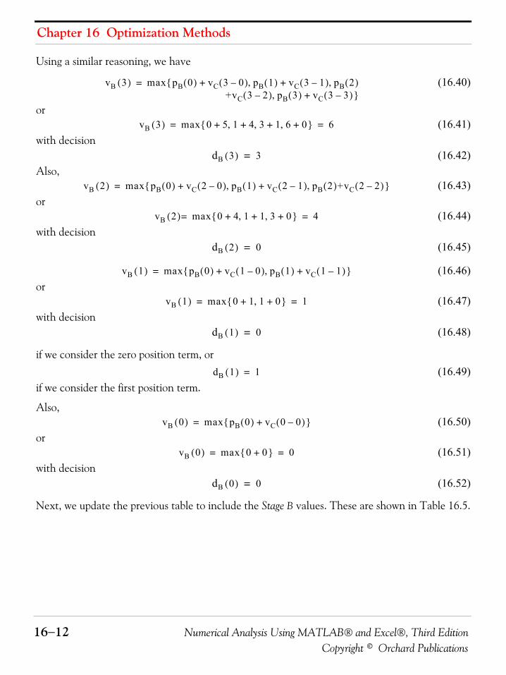
Chapter 16 Optimization Methods
16−12 Numerical Analysis Using MATLAB® and Excel®, Third EditionCopyright © Orchard Publications
Using a similar reasoning, we have
(16.40)
or(16.41)
with decision(16.42)
Also,(16.43)
or(16.44)
with decision(16.45)
(16.46)or
(16.47)with decision
(16.48)
if we consider the zero position term, or (16.49)
if we consider the first position term.
Also,(16.50)
or(16.51)
with decision(16.52)
Next, we update the previous table to include the Stage B values. These are shown in Table 16.5.
vB 3( ) max pB 0( ) vC 3 0–( )+ pB 1( ) vC 3 1–( ) pB 2( )+vC 3 2–( ) pB 3( ) vC 3 3–( )+,
,+,{}
=
vB 3( ) max 0 5 1 4 3 1 6 0+,+,+,+{ } 6= =
dB 3( ) 3=
vB 2( ) max pB 0( ) vC 2 0–( )+ pB 1( ) vC 2 1–( ) pB 2( )+vC 2 2–( ),+,{ }=
vB 2( ) max 0 4 1 1 3 0+,+,+{ }= 4=
dB 2( ) 0=
vB 1( ) max pB 0( ) vC 1 0–( )+ pB 1( ) vC 1 1–( )+,{ }=
vB 1( ) max 0 1 1 0+,+{ } 1= =
dB 1( ) 0=
dB 1( ) 1=
vB 0( ) max pB 0( ) vC 0 0–( )+{ }=
vB 0( ) max 0 0+{ } 0= =
dB 0( ) 0=
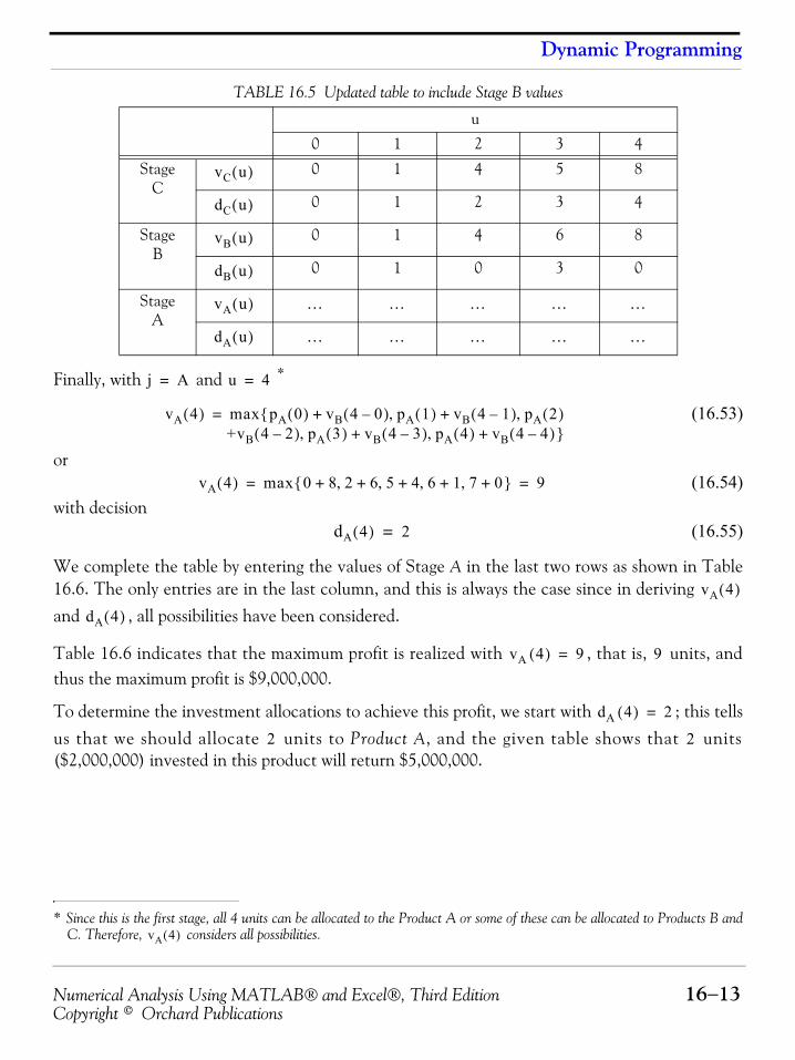
Numerical Analysis Using MATLAB® and Excel®, Third Edition 16−13Copyright © Orchard Publications
Dynamic Programming
Finally, with and *
(16.53)
or(16.54)
with decision(16.55)
We complete the table by entering the values of Stage A in the last two rows as shown in Table16.6. The only entries are in the last column, and this is always the case since in deriving and , all possibilities have been considered.
Table 16.6 indicates that the maximum profit is realized with , that is, units, andthus the maximum profit is $9,000,000.
To determine the investment allocations to achieve this profit, we start with ; this tellsus that we should allocate units to Product A, and the given table shows that units($2,000,000) invested in this product will return $5,000,000.
TABLE 16.5 Updated table to include Stage B values
u
0 1 2 3 4
StageC
0 1 4 5 8
0 1 2 3 4
StageB
0 1 4 6 8
0 1 0 3 0
StageA
* Since this is the first stage, all 4 units can be allocated to the Product A or some of these can be allocated to Products B andC. Therefore, considers all possibilities.
vC u( )
dC u( )
vB u( )
dB u( )
vA u( ) … … … … …
dA u( ) … … … … …
j A= u 4=
vA 4( )
vA 4( ) max pA 0( ) vB 4 0–( )+ pA 1( ) vB 4 1–( ) pA 2( )+vB 4 2–( ) pA 3( ) vB 4 3–( ) pA 4( ) vB 4 4–( )+,+,
,+,{}
=
vA 4( ) max 0 8 2 6 5 4 6 1 7 0+,+,+,+,+{ } 9= =
dA 4( ) 2=
vA 4( )
dA 4( )
vA 4( ) 9= 9
dA 4( ) 2=
2 2
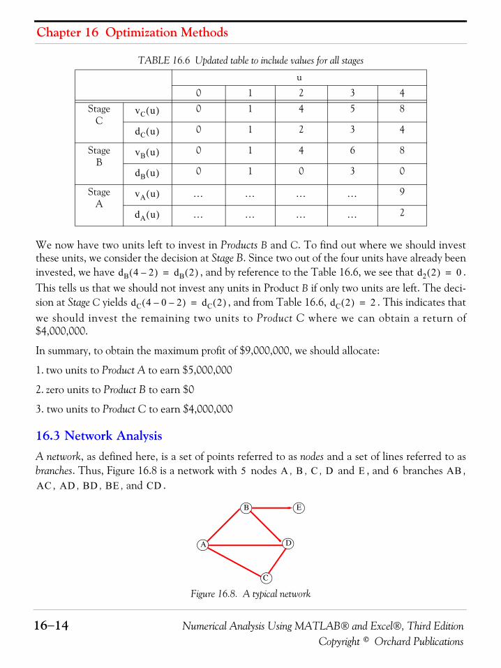
Chapter 16 Optimization Methods
16−14 Numerical Analysis Using MATLAB® and Excel®, Third EditionCopyright © Orchard Publications
We now have two units left to invest in Products B and C. To find out where we should investthese units, we consider the decision at Stage B. Since two out of the four units have already beeninvested, we have , and by reference to the Table 16.6, we see that .This tells us that we should not invest any units in Product B if only two units are left. The deci-sion at Stage C yields , and from Table 16.6, . This indicates thatwe should invest the remaining two units to Product C where we can obtain a return of$4,000,000.
In summary, to obtain the maximum profit of $9,000,000, we should allocate:
1. two units to Product A to earn $5,000,000
2. zero units to Product B to earn $0
3. two units to Product C to earn $4,000,000
16.3 Network AnalysisA network, as defined here, is a set of points referred to as nodes and a set of lines referred to asbranches. Thus, Figure 16.8 is a network with nodes , , , and , and branches ,
, , , , and .
Figure 16.8. A typical network
TABLE 16.6 Updated table to include values for all stages
u
0 1 2 3 4
StageC
0 1 4 5 8
0 1 2 3 4
StageB
0 1 4 6 8
0 1 0 3 0
StageA
9
2
vC u( )
dC u( )
vB u( )
dB u( )
vA u( ) … … … …
dA u( ) … … … …
dB 4 2–( ) dB 2( )= d2 2( ) 0=
dC 4 0– 2–( ) dC 2( )= dC 2( ) 2=
5 A B C D E 6 ABAC AD BD BE CD
A
C
B
D
E
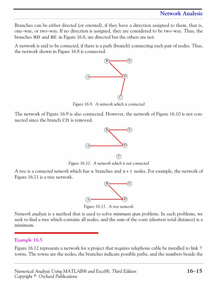
Numerical Analysis Using MATLAB® and Excel®, Third Edition 16−15Copyright © Orchard Publications
Network Analysis
Branches can be either directed (or oriented), if they have a direction assigned to them, that is,one−way, or two−way. If no direction is assigned, they are considered to be two−way. Thus, thebranches and in Figure 16.8, are directed but the others are not.
A network is said to be connected, if there is a path (branch) connecting each pair of nodes. Thus,the network shown in Figure 16.8 is connected.
Figure 16.9. A network which is connected
The network of Figure 16.9 is also connected. However, the network of Figure 16.10 is not con-nected since the branch is removed.
Figure 16.10. A network which is not connected
A tree is a connected network which has branches and nodes. For example, the network ofFigure 16.11 is a tree network.
Figure 16.11. A tree network
Network analysis is a method that is used to solve minimum span problems. In such problems, weseek to find a tree which contains all nodes, and the sum of the costs (shortest total distance) is aminimum.
Example 16.5
Figure 16.12 represents a network for a project that requires telephone cable be installed to link towns. The towns are the nodes, the branches indicate possible paths, and the numbers beside the
BD BE
A
C
B
D
E
CD
A
C
B
D
E
n n 1+
A
B
D
E
7
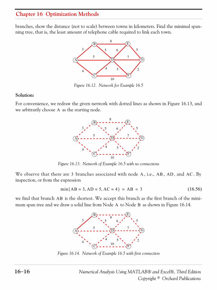
Chapter 16 Optimization Methods
16−16 Numerical Analysis Using MATLAB® and Excel®, Third EditionCopyright © Orchard Publications
branches, show the distance (not to scale) between towns in kilometers. Find the minimal span-ning tree, that is, the least amount of telephone cable required to link each town.
Figure 16.12. Network for Example 16.5
Solution:
For convenience, we redraw the given network with dotted lines as shown in Figure 16.13, andwe arbitrarily choose as the starting node.
Figure 16.13. Network of Example 16.5 with no connections
We observe that there are branches associated with node , i.e., , , and . Byinspection, or from the expression
(16.56)
we find that branch is the shortest. We accept this branch as the first branch of the mini-mum span tree and we draw a solid line from Node to Node as shown in Figure 16.14.
Figure 16.14. Network of Example 16.5 with first connection
A
C
B
D
E
G
F
5
3
4
5
8
7
5
254
10
6
A
A
C
B
D
E
G
F
5
3
4
5
8
7
5
254
10
6
3 A AB AD AC
min AB 3 AD 5 AC 4=,=,={ } AB 3= =
ABA B
A
C
B
D
E
G
F
5
3
4
58
7
5
25410
6
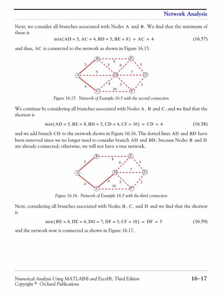
Numerical Analysis Using MATLAB® and Excel®, Third Edition 16−17Copyright © Orchard Publications
Network Analysis
Next, we consider all branches associated with Nodes and . We find that the minimum ofthese is
(16.57)
and thus, is connected to the network as shown in Figure 16.15.
Figure 16.15. Network of Example 16.5 with the second connection
We continue by considering all branches associated with Nodes , and , and we find that theshortest is
(16.58)
and we add branch to the network shown in Figure 16.16. The dotted lines and havebeen removed since we no longer need to consider branch and , because Nodes and are already connected; otherwise, we will not have a tree network.
Figure 16.16. Network of Example 16.5 with the third connection
Next, considering all branches associated with Nodes , , and and we find that the shortestis
(16.59)
and the network now is connected as shown in Figure 16.17.
A B
min AD 5 AC 4 BD 5 BE 8=,=,=,={ } AC 4= =
AC
A
C
B
D
E
G
F
5
3
4
58
7
5
254
10
6
A B C
min AD 5 BE 8 BD 5 CD 4 CF 10=,=,=,=,={ } CD 4= =
CD AD BDAD BD B D
A
C
B
D
E
G
F
3
4
8
7
5
25410
6
B C D
min BE 8 DE 6 DG 7= DF 5= CF, , 10=,=,={ } DF 5= =

Chapter 16 Optimization Methods
16−18 Numerical Analysis Using MATLAB® and Excel®, Third EditionCopyright © Orchard Publications
Figure 16.17. Network of Example 16.5 with the fourth connection
Continuing, we obtain
(16.60)
and the network is connected as shown in Figure 16.18
Figure 16.18. Network of Example 16.5 with the fifth connection
The last step is to determine the shortest branch to Node . We find that
(16.61)
and the complete minimum span tree is shown in Figure 16.19.
Figure 16.19. Network of Example 16.5 with all connections
Figure 16.19 shows that the minimum distance is kilometers.
A
C
B
D
E
G
F
3
4
8
7
5
254
6
min BE 8 DE 6 DG 7=,=,={ } DE 6= =
A
C
B
D
E
G
F
3
4
7
5
254
6
G
min EG 5 DG 7 FG 2=,=,={ } FG 2= =
A
C
B
D
E
G
F
3
4 254
6
3 4 4 6 5 2+ + + + + 24=
Numerical Analysis Using MATLAB® and Excel®, Third Edition 16−19Copyright © Orchard Publications
Summary
16.4 Summary• Linear programming is a procedure we follow to maximize or minimize a particular quantity,
referred to as the objective, which is dependent on a finite number of variables. These variablesmay or may not be independent of each another, and in most cases are subject to certain con-ditions or limitations referred to as constraints.
• Dynamic Programming is based on R. Bellman’s Principle of Optimality which states that anoptimum policy has the property that whatever the initial state and the initial decisions are,the remaining decisions must constitute an optimum policy with regard to the state resultingfrom the first decision.
• A network, as defined in this chapter, is a set of points referred to as nodes and a set of linesreferred to as branches.
• A tree is a connected network which has branches and nodes.
• Network analysis is a method that is used to solve minimum span problems. In such problems, weseek to find a tree which contains all nodes, and the sum of the costs (shortest total distance) isa minimum.
n n 1+
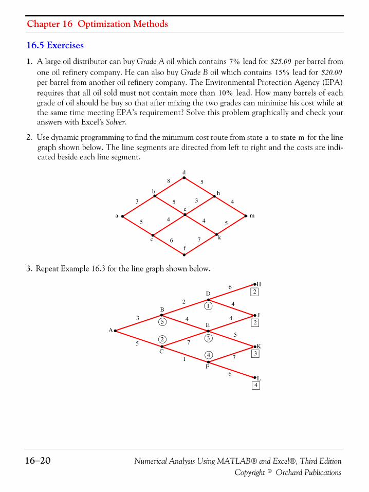
Chapter 16 Optimization Methods
16−20 Numerical Analysis Using MATLAB® and Excel®, Third EditionCopyright © Orchard Publications
16.5 Exercises
1. A large oil distributor can buy Grade A oil which contains lead for per barrel fromone oil refinery company. He can also buy Grade B oil which contains lead for per barrel from another oil refinery company. The Environmental Protection Agency (EPA)requires that all oil sold must not contain more than lead. How many barrels of eachgrade of oil should he buy so that after mixing the two grades can minimize his cost while atthe same time meeting EPA’s requirement? Solve this problem graphically and check youranswers with Excel’s Solver.
2. Use dynamic programming to find the minimum cost route from state to state for the linegraph shown below. The line segments are directed from left to right and the costs are indi-cated beside each line segment.
3. Repeat Example 16.3 for the line graph shown below.
7% $25.0015% $20.00
10%
a m
k
h
f
d
e
c
b
ma
3
6
3
4
5
5
58
7
5
4
4
A
B
D
H
C
F
L
E
J
K3
2
2
4
5
1
2 3
4
3
5
1
6
2
6
4
4
5
7
4
7
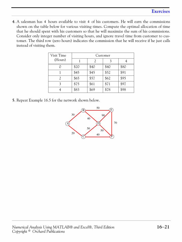
Numerical Analysis Using MATLAB® and Excel®, Third Edition 16−21Copyright © Orchard Publications
Exercises
4. A salesman has hours available to visit of his customers. He will earn the commissionsshown on the table below for various visiting times. Compute the optimal allocation of timethat he should spent with his customers so that he will maximize the sum of his commissions.Consider only integer number of visiting hours, and ignore travel time from customer to cus-tomer. The third row (zero hours) indicates the commission that he will receive if he just callsinstead of visiting them.
5. Repeat Example 16.5 for the network shown below.
Visit Time(Hours)
Customer
1 2 3 4
0 $20 $40 $40 $80
1 $45 $45 $52 $91
2 $65 $57 $62 $95
3 $75 $61 $71 $97
4 $83 $69 $78 $98
4 4
A
C
B
D
E
F
30
20
40
50
70
40
90
5050
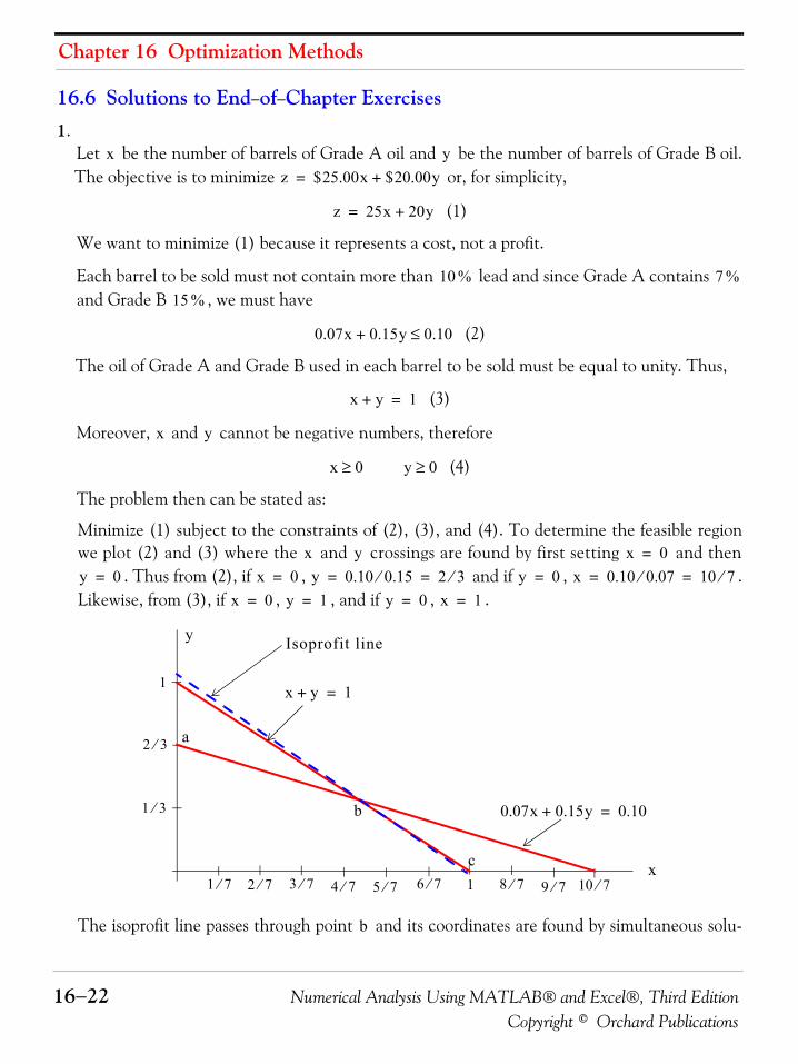
Chapter 16 Optimization Methods
16−22 Numerical Analysis Using MATLAB® and Excel®, Third EditionCopyright © Orchard Publications
16.6 Solutions to End−of−Chapter Exercises1.
Let be the number of barrels of Grade A oil and be the number of barrels of Grade B oil.The objective is to minimize or, for simplicity,
(1)
We want to minimize (1) because it represents a cost, not a profit.
Each barrel to be sold must not contain more than lead and since Grade A contains and Grade B , we must have
(2)
The oil of Grade A and Grade B used in each barrel to be sold must be equal to unity. Thus,
(3)
Moreover, and cannot be negative numbers, therefore
(4)
The problem then can be stated as:
Minimize (1) subject to the constraints of (2), (3), and (4). To determine the feasible regionwe plot (2) and (3) where the and crossings are found by first setting and then
. Thus from (2), if , and if , .Likewise, from (3), if , , and if , .
The isoprofit line passes through point and its coordinates are found by simultaneous solu-
x yz $25.00x $20.00y+=
z 25x 20y+=
10 % 7 %15 %
0.07x 0.15y 0.10≤+
x y+ 1=
x y
x 0≥ y 0≥
x y x 0=
y 0= x 0= y 0.10 0.15⁄ 2 3⁄= = y 0= x 0.10 0.07⁄ 10 7⁄= =
x 0= y 1= y 0= x 1=
x
y
1
1
a2 3⁄
1 3⁄
10 7⁄9 7⁄8 7⁄6 7⁄5 7⁄4 7⁄3 7⁄2 7⁄1 7⁄
b
c
x y+ 1=
0.07x 0.15y+ 0.10=
Isoprofit line
b
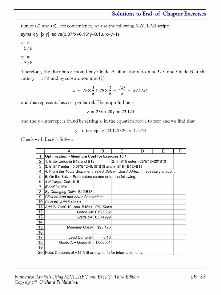
Numerical Analysis Using MATLAB® and Excel®, Third Edition 16−23Copyright © Orchard Publications
Solutions to End−of−Chapter Exercises
tion of (2) and (3). For convenience, we use the following MATLAB script:
syms x y; [x,y]=solve(0.07*x+0.15*y−0.10, x+y−1)
x = 5/8
y = 3/8
Therefore, the distributor should buy Grade A oil at the ratio and Grade B at theratio and by substitution into (1)
and this represents his cost per barrel. The isoprofit line is
and the −intercept is found by setting in the equation above to zero and we find that
Check with Excel’s Solver:
x 5 8⁄=
y 3 8⁄=
z 25 58---× 20 3
8---×+ 185
8--------- $23.125= = =
z 25x 20y+ 23.125= =
y x
y intercept– 23.125 20⁄ 1.1563= =
1234567891011121314151617181920
A B C D E FOptimization - Minimum Cost for Exercise 16.11. Enter zeros in B12 and B13 2. In B15 enter =25*B12+20*B133. In B17 enter =0.07*B12+0.15*B13 and in B18 =B12+B134. From the Tools drop menu select Solver . Use Add-Ins if necessary to add it.5. On the Solver Parameters screen enter the following:Set Target Cell: B15Equal to: MinBy Changing Cells: B12:B13Click on Add and enter Constraints:B12>=0, Add B13>=0,Add B17<=0.10, Add B18=1, OK , Solve
Grade A= 0.625002Grade B= 0.374999
Minimum Cost= $23.125
Lead Content= 0.10Grade A + Grade B= 1.000001
Note: Contents of A12:A18 are typed-in for information only
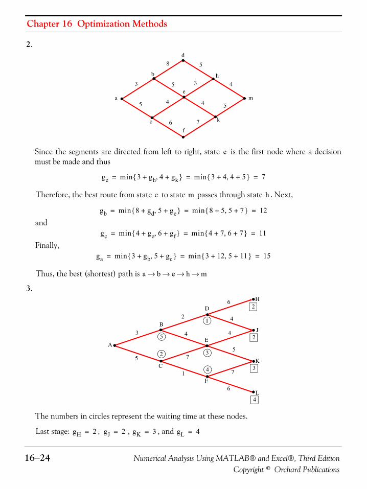
Chapter 16 Optimization Methods
16−24 Numerical Analysis Using MATLAB® and Excel®, Third EditionCopyright © Orchard Publications
2.
Since the segments are directed from left to right, state is the first node where a decisionmust be made and thus
Therefore, the best route from state to state passes through state . Next,
and
Finally,
Thus, the best (shortest) path is
3.
The numbers in circles represent the waiting time at these nodes.
Last stage: , , , and
k
h
f
d
e
c
b
ma
3
6
3
4
5
5
58
7
5
4
4
e
ge min 3 gh 4 gk+,+{ } min 3 4 4 5+,+{ } 7= = =
e m h
gb min 8 gd 5 ge+,+{ } min 8 5 5 7+,+{ } 12= = =
gc min 4 ge 6 gf+,+{ } min 4 7 6 7+,+{ } 11= = =
ga min 3 gb 5 gc+,+{ } min 3 12 5 11+,+{ } 15= = =
a b e h m→ → → →
A
B
D
H
C
F
L
E
J
K3
2
2
4
5
1
2 3
4
3
5
1
6
2
6
4
4
5
7
4
7
gH 2= gJ 2= gK 3= gL 4=
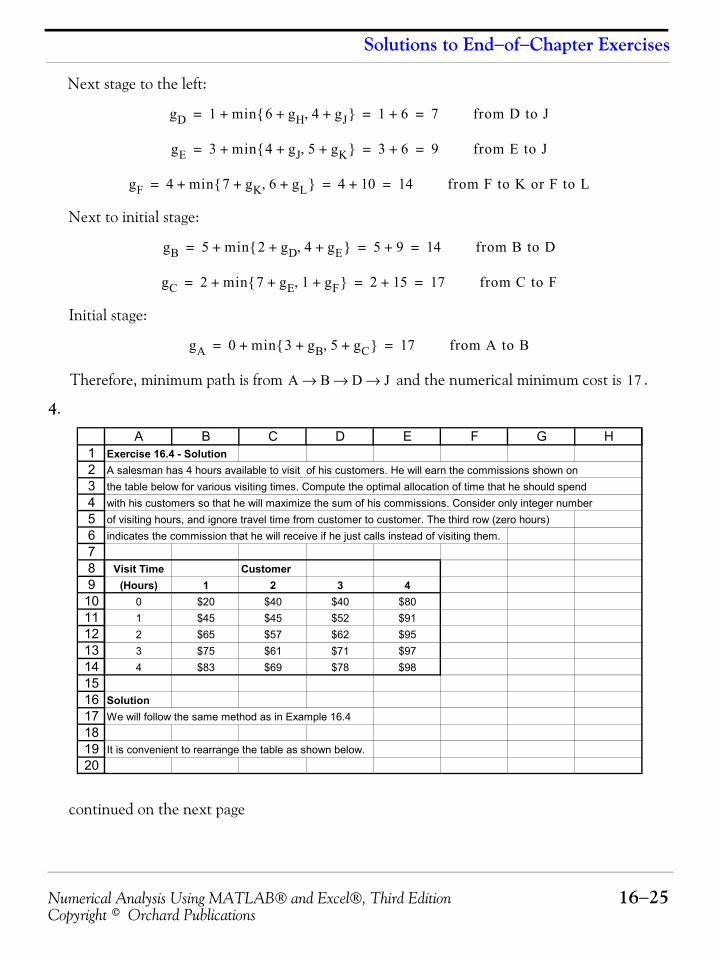
Numerical Analysis Using MATLAB® and Excel®, Third Edition 16−25Copyright © Orchard Publications
Solutions to End−of−Chapter Exercises
Next stage to the left:
Next to initial stage:
Initial stage:
Therefore, minimum path is from and the numerical minimum cost is .
4.
continued on the next page
gD 1 min 6 gH 4 gJ+,+{ }+ 1 6+ 7 from D to J= = =
gE 3 min 4 gJ 5 gK+,+{ }+ 3 6+ 9 from E to J= = =
gF 4 min 7 gK 6 gL+,+{ }+ 4 10+ 14 from F to K or F to L= = =
gB 5 min 2 gD 4 gE+,+{ }+ 5 9+ 14 from B to D= = =
gC 2 min 7 gE 1 gF+,+{ }+ 2 15+ 17 from C to F= = =
gA 0 min 3 gB 5 gC+,+{ }+ 17 from A to B= =
A B D J→ → → 17
1234567891011121314151617181920
A B C D E F G HExercise 16.4 - SolutionA salesman has 4 hours available to visit of his customers. He will earn the commissions shown on the table below for various visiting times. Compute the optimal allocation of time that he should spend with his customers so that he will maximize the sum of his commissions. Consider only integer number of visiting hours, and ignore travel time from customer to customer. The third row (zero hours) indicates the commission that he will receive if he just calls instead of visiting them.
Visit Time Customer(Hours) 1 2 3 4
0 $20 $40 $40 $801 $45 $45 $52 $912 $65 $57 $62 $953 $75 $61 $71 $974 $83 $69 $78 $98
SolutionWe will follow the same method as in Example 16.4
It is convenient to rearrange the table as shown below.
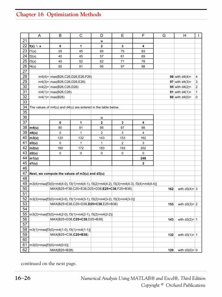
Chapter 16 Optimization Methods
16−26 Numerical Analysis Using MATLAB® and Excel®, Third EditionCopyright © Orchard Publications
continued on the next page.
212223242526272829303132333435363738394041424344454647484950515253545556575859606162
A B C D E F G H Iu
f(x) \ x 0 1 2 3 4f1(x) 20 45 65 75 83f2(x) 40 45 57 61 69f3(x) 40 52 62 71 78f4(x) 80 91 95 97 98
m4(4)= max(B26,C26,D26,E26,F26) 98 with d4(4)= 4m4(3)= max(B26,C26,D26,E26) 97 with d4(3)= 3m4(2)= max(B26,C26,D26) 95 with d4(2)= 2m4(1)= max(B26,C26) 91 with d4(1)= 1m4(1)= max(B26) 80 with d4(0)= 0
The values of m4(u) and d4(u) are entered in the table below.
u0 1 2 3 4
m4(u) 80 91 95 97 98d4(u) 0 1 2 3 4m3(u) 120 132 143 153 162d3(u) 0 1 1 2 3m2(u) 160 172 183 193 202d2(u) 0 0 0 0 0m1(u) 248d1(u) 2
Next, we compute the values of m3(u) and d3(u)
m3(4)=max[f3(0)+m4(4-0), f3(1)+m4(4-1), f3(2)+m4(4-2), f3(3)+m4(4-3), f3(4)+m4(4-4)]MAX(B25+F38,C25+E38,D25+D38,E25+C38,F25+B38) 162 with d3(4)= 3
m3(3)=max[f3(0)+m4(3-0), f3(1)+m4(3-1), f3(2)+m4(3-2), f3(3)+m4(3-3)]MAX(B25+E38,C25+D38,D25+C38,E25+B38) 153 with d3(3)= 2
m3(2)=max[f3(0)+m4(2-0), f3(1)+m4(2-1), f3(2)+m4(2-2)]MAX(B25+D38,C25+C38,D25+B38) 143 with d3(2)= 1
m3(1)=max[f3(0)+m4(1-0), f3(1)+m4(1-1)]MAX(B25+C38,C25+B38) 132 with d3(1)= 1
m3(0)=max[f3(0)+m4(0-0)]MAX(B25+B38) 120 with d3(0)= 0
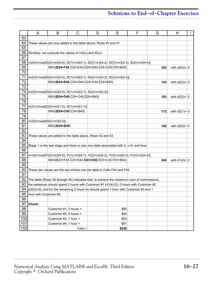
Numerical Analysis Using MATLAB® and Excel®, Third Edition 16−27Copyright © Orchard Publications
Solutions to End−of−Chapter Exercises
63646566676869707172737475767778798081828384858687888990919293949596979899100101102
A B C D E F G H I
These values are now added to the table above, Rows 40 and 41
Similarly, we compute the values of m2(u) and d2(u)
m2(4)=max[f2(0)+m3(4-0), f2(1)+m3(4-1), f2(2)+m3(4-2), f2(3)+m3(4-3), f2(4)+m3(4-4)]MAX(B24+F40,C24+E40,D24+D40,E24+C40,F25+B40) 202 with d2(4)= 0
m2(3)=max[f2(0)+m3(3-0), f2(1)+m3(3-1), f2(2)+m3(3-2), f2(3)+m3(3-3)]MAX(B24+E40,C24+D40,D24+C40,E24+B40) 193 with d2(3)= 0
m2(2)=max[f2(0)+m3(2-0), f2(1)+m3(2-1), f2(2)+m3(2-2)]MAX(B24+D40,C24+C40,D24+B40) 183 with d2(2)= 0
m2(1)=max[f2(0)+m3(1-0), f2(1)+m3(1-1)]MAX(B24+C40,C24+B40) 172 with d2(1)= 0
m2(0)=max[f2(0)+m3(0-0)]MAX(B24+B40) 160 with d2(0)= 0
These values are added to the table above, Rows 42 and 43
Stage 1 is the last stage and there is only one state associated with it, u=4, and thus
m1(4)=max[f1(0)+m2(4-0), f1(1)+m2(4-1), f1(2)+m2(4-2), f1(3)+m2(4-3), f1(4)+m2(4-4)]MAX(B23+F42,C23+E42,D23+D42,E23+C42,F23+B42) 248 with d1(4)= 2
These two values are the last entries into the table in Cells F44 and F45
The table (Rows 36 through 45) indicates that, to achieve the maximum sum of commissions, the salesman should spend 2 hours with Customer #1 (d1(4)=2), 0 hours with Customer #2 (d2(4)=0), and for the remaining 2 hours he should spend 1 hour with Customer #3 and 1hour with Customer #4.
Check:Customer #1, 2 hours = $65Customer #2, 0 hours = $40Customer #3, 1 hour = $52Customer #4, 1 hour = $91
Total = $248
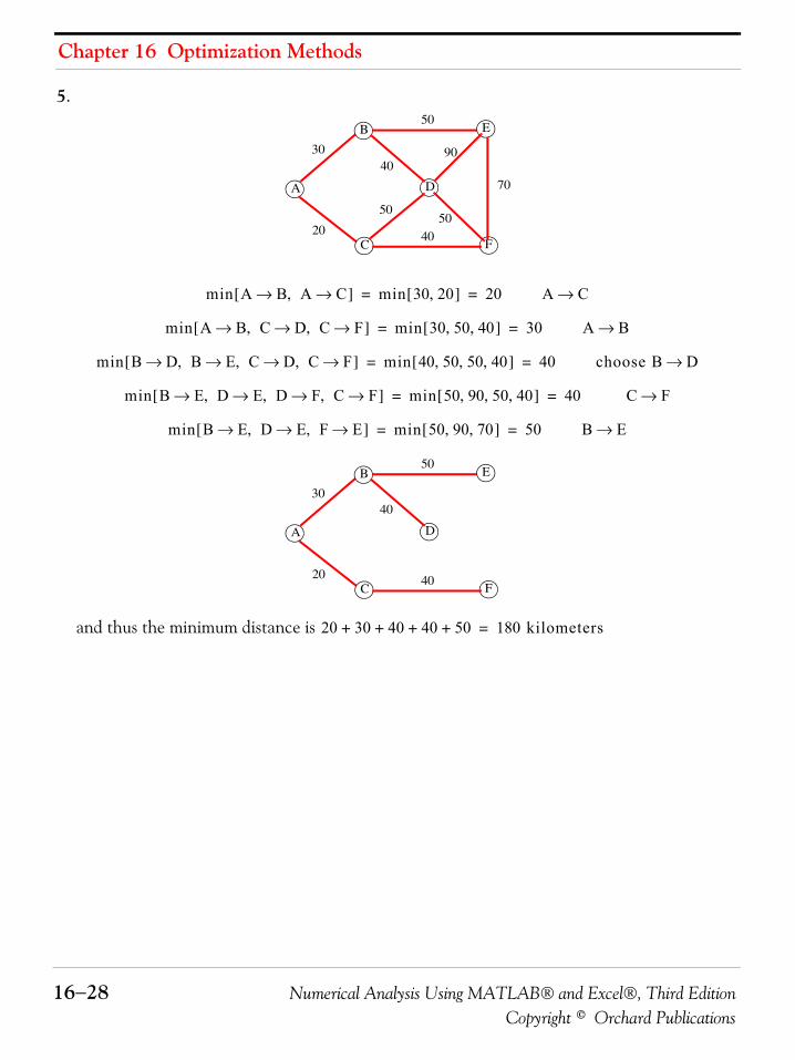
Chapter 16 Optimization Methods
16−28 Numerical Analysis Using MATLAB® and Excel®, Third EditionCopyright © Orchard Publications
5.
and thus the minimum distance is
A
C
B
D
E
F
30
20
40
50
70
40
90
5050
min A B A C→,→[ ] min 30 20,[ ] 20= = A C→
min A B C D C F→,→,→[ ] min 30 50 40, ,[ ] 30= = A B→
min B D B E C D C F→,→,→,→[ ] min 40 50 50 40, , ,[ ] 40= = choose B D→
min B E D E D F C F→,→,→,→[ ] min 50 90 50 40, , ,[ ] 40= = C F→
min B E D E F E→,→,→[ ] min 50 90 70, ,[ ] 50= = B E→
A
C
B
D
E
F
30
20
50
40
40
20 30 40 40 50+ + + + 180 kilometers=
Numerical Analysis Using MATLAB® and Excel®, Third Edition A−1Copyright © Orchard Publications
Appendix A
Difference Equations in Discrete−Time Systems
his appendix is a treatment of linear difference equations with constant coefficients and it isconfined to first− and second−order difference equations and their solution. Higher−orderdifference equations of this type and their solution is facilitated with the Z−transform.*
A.1 Recursive Method for Solving Difference Equations
In mathematics, a recursion is an expression, such as a polynomial, each term of which is deter-mined by application of a formula to preceding terms. The solution of a difference equation isoften obtained by recursive methods. An example of a recursive method is Newton’s method† forsolving non−linear equations. While recursive methods yield a desired result, they do not providea closed−form solution. If a closed−form solution is desired, we can solve difference equationsusing the Method of Undetermined Coefficients, and this method is similar to the classicalmethod of solving linear differential equations with constant coefficients. This method isdescribed in the next section.
A.2 Method of Undetermined CoefficientsA second−order difference equation has the form
(A.1)
where and are constants and the right side is some function of . This difference equationexpresses the output at time as the linear combination of two previous outputs and . The right side of relation (A.1) is referred to as the forcing function. The general(closed-form) solution of relation (A.1) is the same as that used for solving second−order differen-tial equations. The three steps are as follows:
1. Obtain the natural response (complementary solution) in terms of two arbitrary realconstants and , where and are also real constants, that is,
(A.2)
2. Obtain the forced response (particular solution) in terms of an arbitrary real constant ,
* For an introduction and applications of the Z-transform please refer to Signals and Systems with MATLABComputing and Simulink Modeling, Third Edition, ISBN 0-9744239-9-8.
† Newton’s method is discussed in Chapter 2.
T
y n( ) a1y n 1–( ) a2 n 2–( )+ + f n( )=
a1 a2 ny n( ) n y n 1–( )
y n 2–( )
yC n( )k1 k2 a1 a2
yC n( ) k1a1n k2a2
n+=
yP n( ) k3
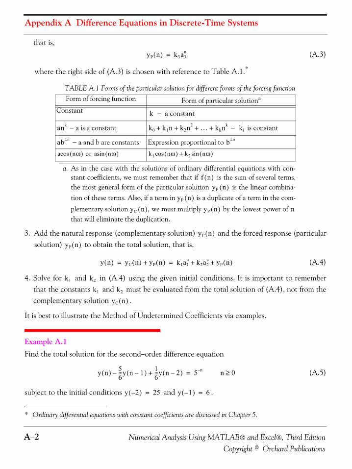
Appendix A Difference Equations in Discrete-Time Systems
A−2 Numerical Analysis Using MATLAB® and Excel®, Third EditionCopyright © Orchard Publications
that is,(A.3)
where the right side of (A.3) is chosen with reference to Table A.1.*
3. Add the natural response (complementary solution) and the forced response (particularsolution) to obtain the total solution, that is,
(A.4)
4. Solve for and in (A.4) using the given initial conditions. It is important to rememberthat the constants and must be evaluated from the total solution of (A.4), not from thecomplementary solution .
It is best to illustrate the Method of Undetermined Coefficients via examples.
Example A.1 Find the total solution for the second−order difference equation
(A.5)
subject to the initial conditions and .
* Ordinary differential equations with constant coefficients are discussed in Chapter 5.
TABLE A.1 Forms of the particular solution for different forms of the forcing functionForm of forcing function Form of particular solutiona
a. As in the case with the solutions of ordinary differential equations with con-stant coefficients, we must remember that if is the sum of several terms,the most general form of the particular solution is the linear combina-tion of these terms. Also, if a term in is a duplicate of a term in the com-
plementary solution , we must multiply by the lowest power of that will eliminate the duplication.
Constant − a constant
− a is a constant − is constant
− a and b are constants Expression proportional to
yP n( ) k3a3n=
f n( )yP n( )
yP n( )yC n( ) yP n( ) n
k
ank k0 k1n k2n2 … kknk+ + + + ki
ab n± b n±
nω( ) or nω( )asinacos k1 nω( )cos k2 nω( )sin+
yC n( )yP n( )
y n( ) yC n( ) yP n( )+ k1a1n k2a2
n yP n( )+ += =
k1 k2
k1 k2
yC n( )
y n( ) 56---y n 1–( ) 1
6---y n 2–( )+– 5 n–= n 0≥
y 2–( ) 25= y 1–( ) 6=
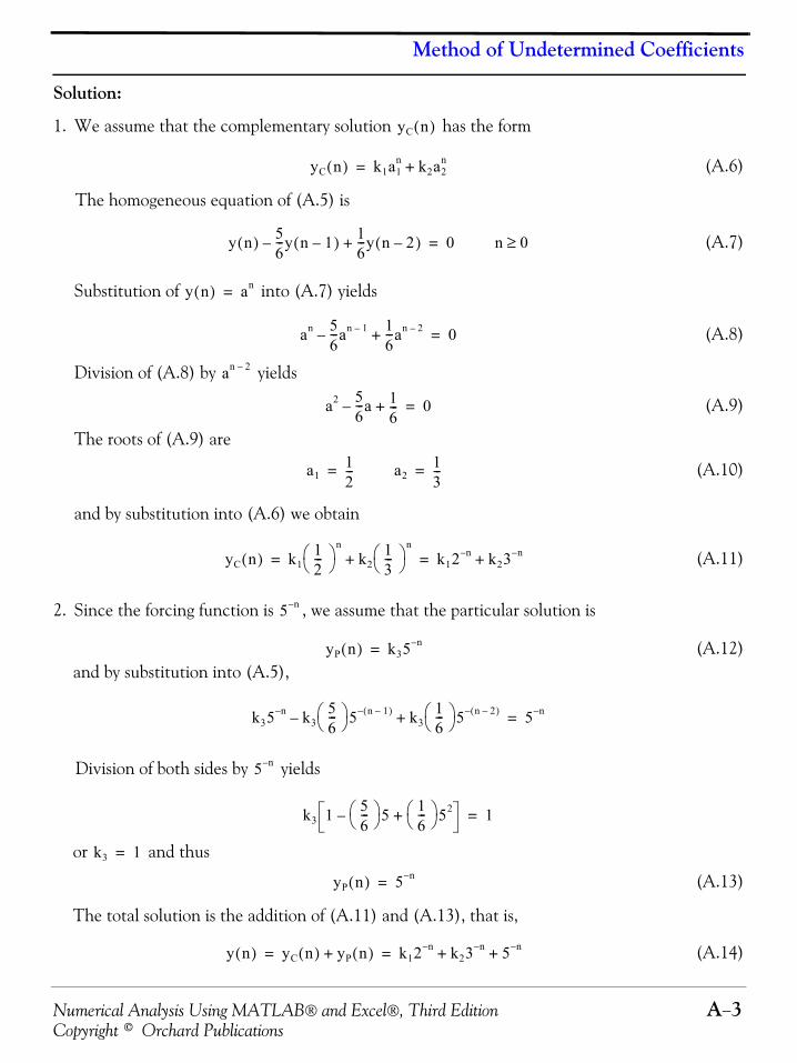
Numerical Analysis Using MATLAB® and Excel®, Third Edition A−3Copyright © Orchard Publications
Method of Undetermined Coefficients
Solution:
1. We assume that the complementary solution has the form
(A.6)
The homogeneous equation of (A.5) is
(A.7)
Substitution of into (A.7) yields
(A.8)
Division of (A.8) by yields
(A.9)
The roots of (A.9) are
(A.10)
and by substitution into (A.6) we obtain
(A.11)
2. Since the forcing function is , we assume that the particular solution is
(A.12)and by substitution into (A.5),
Division of both sides by yields
or and thus
(A.13)
The total solution is the addition of (A.11) and (A.13), that is,
(A.14)
yC n( )
yC n( ) k1a1n k2a2
n+=
y n( ) 56---y n 1–( ) 1
6---y n 2–( )+– 0= n 0≥
y n( ) an=
an 56---an 1––
16---an 2–+ 0=
an 2–
a2 56---a– 1
6---+ 0=
a112---= a2
13---=
yC n( ) k112---⎝ ⎠
⎛ ⎞n
k213---⎝ ⎠
⎛ ⎞n
+ k12 n– k23 n–+= =
5 n–
yP n( ) k35 n–=
k35 n– k356---⎝ ⎠
⎛ ⎞ 5 n 1–( )–– k316---⎝ ⎠
⎛ ⎞ 5 n 2–( )–+ 5 n–=
5 n–
k3 1 56---⎝ ⎠
⎛ ⎞ 5–16---⎝ ⎠
⎛ ⎞ 52+ 1=
k3 1=
yP n( ) 5 n–=
y n( ) yC n( ) yP n( )+ k12 n– k23 n– 5 n–+ += =
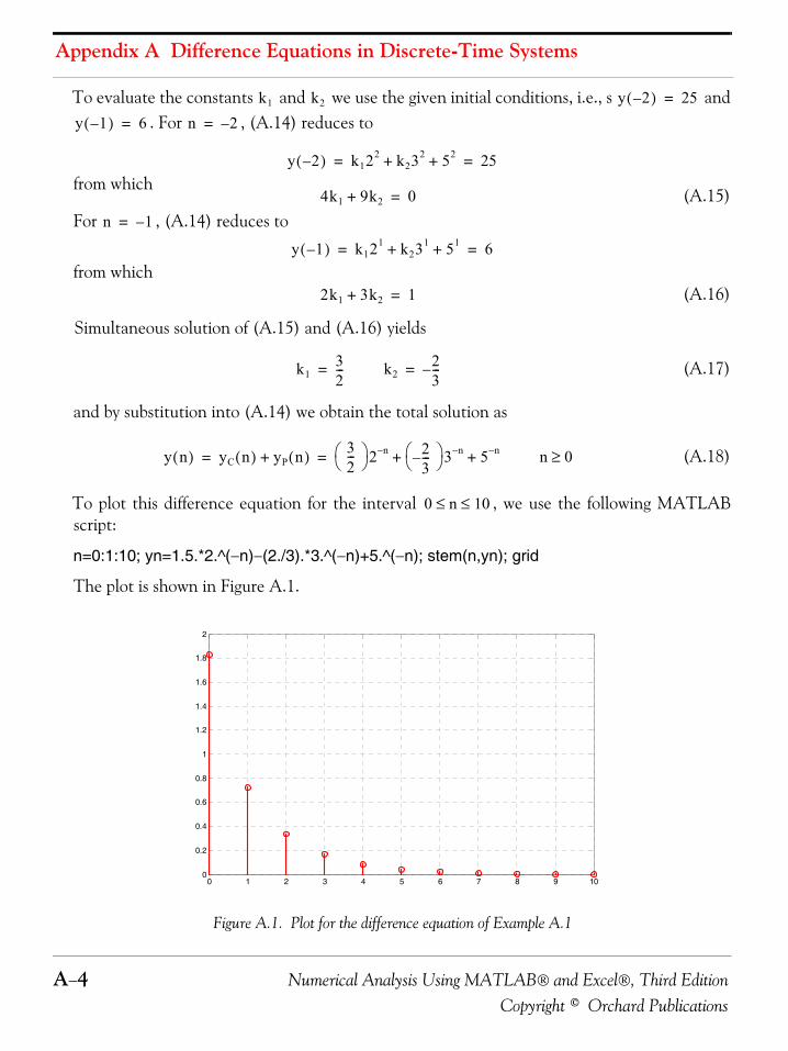
Appendix A Difference Equations in Discrete-Time Systems
A−4 Numerical Analysis Using MATLAB® and Excel®, Third EditionCopyright © Orchard Publications
To evaluate the constants and we use the given initial conditions, i.e., s and. For , (A.14) reduces to
from which(A.15)
For , (A.14) reduces to
from which(A.16)
Simultaneous solution of (A.15) and (A.16) yields
(A.17)
and by substitution into (A.14) we obtain the total solution as
(A.18)
To plot this difference equation for the interval , we use the following MATLABscript:
n=0:1:10; yn=1.5.*2.^(−n)−(2./3).*3.^(−n)+5.^(−n); stem(n,yn); grid
The plot is shown in Figure A.1.
Figure A.1. Plot for the difference equation of Example A.1
k1 k2 y 2–( ) 25=
y 1–( ) 6= n 2–=
y 2–( ) k122 k232 52+ + 25= =
4k1 9k2+ 0=
n 1–=
y 1–( ) k121 k231 51+ + 6= =
2k1 3k2+ 1=
k132---= k2
23---–=
y n( ) yC n( ) yP n( )+32---⎝ ⎠
⎛ ⎞ 2 n– 23---–⎝ ⎠
⎛ ⎞ 3 n– 5 n–+ += = n 0≥
0 n 10≤ ≤
0 1 2 3 4 5 6 7 8 9 100
0.2
0.4
0.6
0.8
1
1.2
1.4
1.6
1.8
2
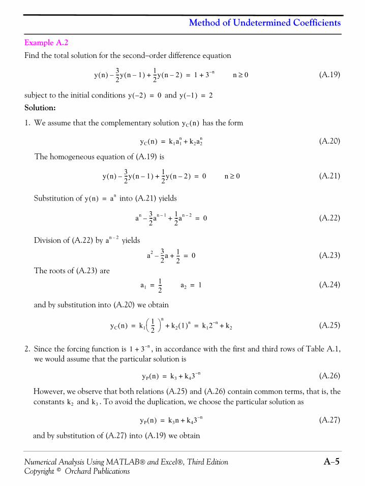
Numerical Analysis Using MATLAB® and Excel®, Third Edition A−5Copyright © Orchard Publications
Method of Undetermined Coefficients
Example A.2 Find the total solution for the second−order difference equation
(A.19)
subject to the initial conditions and
Solution:
1. We assume that the complementary solution has the form
(A.20)
The homogeneous equation of (A.19) is
(A.21)
Substitution of into (A.21) yields
(A.22)
Division of (A.22) by yields
(A.23)
The roots of (A.23) are
(A.24)
and by substitution into (A.20) we obtain
(A.25)
2. Since the forcing function is , in accordance with the first and third rows of Table A.1,we would assume that the particular solution is
(A.26)
However, we observe that both relations (A.25) and (A.26) contain common terms, that is, theconstants and . To avoid the duplication, we choose the particular solution as
(A.27)
and by substitution of (A.27) into (A.19) we obtain
y n( ) 32---y n 1–( ) 1
2---y n 2–( )+– 1 3 n–+= n 0≥
y 2–( ) 0= y 1–( ) 2=
yC n( )
yC n( ) k1a1n k2a2
n+=
y n( ) 32---y n 1–( ) 1
2---y n 2–( )+– 0= n 0≥
y n( ) an=
an 32---an 1–– 1
2---an 2–+ 0=
an 2–
a2 32---a– 1
2---+ 0=
a112---= a2 1=
yC n( ) k112---⎝ ⎠
⎛ ⎞n
k2 1( )n+ k12 n– k2+= =
1 3 n–+
yP n( ) k3 k43 n–+=
k2 k3
yP n( ) k3n k43 n–+=
Appendix A Difference Equations in Discrete-Time Systems
A−6 Numerical Analysis Using MATLAB® and Excel®, Third EditionCopyright © Orchard Publications
Equating like terms, we obtain
and after simplification,
By substitution into (A.27),
(A.28)
The total solution is the addition of (A.25) and (A.28), that is,
(A.29)
To evaluate the constants and we use the given initial conditions, i.e., s and. For , (A.29) reduces to
from which
(A.30)
For , (A.29) reduces to
from which
(A.31)
Simultaneous solution of (A.30) and (A.31) yields
(A.32)
and by substitution into (A.29) we obtain the total solution as
k3n k43 n– 32---⎝ ⎠
⎛ ⎞ k3 n 1–( )– 32---⎝ ⎠
⎛ ⎞ k43 n 1–( )–– 12---k3 n 2–( ) 1
2---⎝ ⎠
⎛ ⎞ k43 n 2–( )–+ + + 1 3 n–+=
k3n k43 n– 32---⎝ ⎠
⎛ ⎞ k3n–32---⎝ ⎠
⎛ ⎞ k392---⎝ ⎠
⎛ ⎞ k43 n––12---k3n k3–
92---⎝ ⎠
⎛ ⎞ k43 n–+ + + + 1 3 n–+=
k43 n– 32---⎝ ⎠
⎛ ⎞ k3 k3–+ 1 3 n–+=
32---⎝ ⎠
⎛ ⎞ k3 k3– 1=
k43 n– 3 n–=
k3 2= k4 1=
yP n( ) 2n 3 n–+=
y n( ) yC n( ) yP n( )+ k12 n– k2 2n 3 n–+ + += =
k1 k2 y 2–( ) 0=
y 1–( ) 2= n 2–=
y 2–( ) k122 k2 4– 9+ + 0= =
4k1 k2+ 5–=
n 1–=
y 1–( ) k121 k2 2– 31+ + 2= =
2k1 k2+ 1=
k1 3–= k2 7=
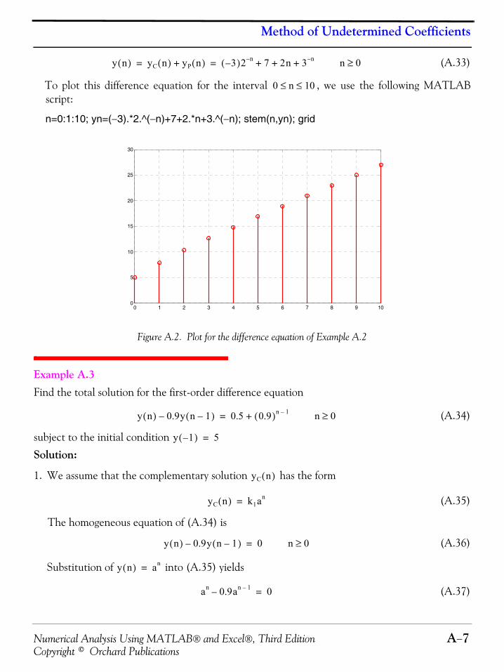
Numerical Analysis Using MATLAB® and Excel®, Third Edition A−7Copyright © Orchard Publications
Method of Undetermined Coefficients
(A.33)
To plot this difference equation for the interval , we use the following MATLABscript:
n=0:1:10; yn=(−3).*2.^(−n)+7+2.*n+3.^(−n); stem(n,yn); grid
Figure A.2. Plot for the difference equation of Example A.2
Example A.3 Find the total solution for the first-order difference equation
(A.34)
subject to the initial condition
Solution:
1. We assume that the complementary solution has the form
(A.35)
The homogeneous equation of (A.34) is
(A.36)
Substitution of into (A.35) yields
(A.37)
y n( ) yC n( ) yP n( )+ 3–( )2 n– 7 2n 3 n–+ + += = n 0≥
0 n 10≤ ≤
0 1 2 3 4 5 6 7 8 9 100
5
10
15
20
25
30
y n( ) 0.9y n 1–( )– 0.5 0.9( )n 1–+= n 0≥
y 1–( ) 5=
yC n( )
yC n( ) k1an=
y n( ) 0.9y n 1–( )– 0= n 0≥
y n( ) an=
an 0.9an 1–– 0=
Appendix A Difference Equations in Discrete-Time Systems
A−8 Numerical Analysis Using MATLAB® and Excel®, Third EditionCopyright © Orchard Publications
Division of (A.37) by yields
(A.38)
and by substitution into (A.35) we obtain
(A.39)
2. Since the forcing function is , in accordance with the first and third rows ofTable A.1, we would assume that the particular solution is
(A.40)
However, we observe that both relations (A.39) and (A.40) contain common terms, that is,the constants and . To avoid the duplication, we choose the particular solu-tion as
(A.41)
and by substitution of (A.41) into (A.34) we obtain
Equating like terms, we obtain
and after simplification,
By substitution into (A.41),
(A.42)
The total solution is the addition of (A.39) and (A.42), that is,
(A.43)
an 1–
a 0.9– 0=
a 0.9=
yC n( ) k1 0.9( )n=
0.5 0.9( )n 1–+
yP n( ) k2 k3 0.9( )n+=
k1 0.9( )n k3 0.9( )n
yP n( ) k2 k3n 0.9( )n+=
k2 k3n 0.9( )n 0.9k2– 0.9k3 n 1–( ) 0.9( ) n 1–( )–+ 0.5 0.9( )n 1–+=
0.1k2 k3n 0.9( )n 0.9k3n 0.9( ) n 1–( )– 0.9k3 0.9( ) n 1–( )+ + 0.5 0.9( )n 1–+=
0.1k2 k3n 0.9( )n 0.9k3n 0.9( )n0.9 1–– 0.9k3 0.9( )n0.9 1–+ + 0.5 0.9( )n 1–+=
0.1k2 k3n 0.9( )n k3n 0.9( )n– k3 0.9( )n+ + 0.5 0.9( )n 1–+ 0.5 0.9( ) 1– 0.9( )n+= =
0.1k2 0.5=
k3 0.9( )n 0.9( ) 1– 0.9( )n=
k2 5= k3109------=
yP n( ) 5 109------n 0.9( )n+=
y n( ) yC n( ) yP n( )+ k1 0.9( ) n 109------n 0.9( )n 5+ += =
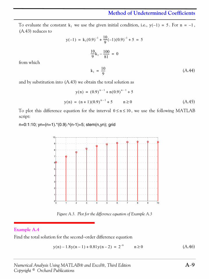
Numerical Analysis Using MATLAB® and Excel®, Third Edition A−9Copyright © Orchard Publications
Method of Undetermined Coefficients
To evaluate the constant we use the given initial condition, i.e., . For ,(A.43) reduces to
from which
(A.44)
and by substitution into (A.43) we obtain the total solution as
(A.45)
To plot this difference equation for the interval , we use the following MATLABscript:
n=0:1:10; yn=(n+1).*(0.9).^(n-1)+5; stem(n,yn); grid
Figure A.3. Plot for the difference equation of Example A.3
Example A.4 Find the total solution for the second−order difference equation
(A.46)
k1 y 1–( ) 5= n 1–=
y 1–( ) k1 0.9( ) 1– 109
------ 1–( ) 0.9( ) 1– 5+ + 5= =
109------k1
10081---------– 0=
k1109------=
y n( ) 0.9( ) n 1– n 0.9( ) n 1– 5+ +=
y n( ) n 1+( ) 0.9( ) n 1– 5+= n 0≥
0 n 10≤ ≤
0 1 2 3 4 5 6 7 8 9 100
1
2
3
4
5
6
7
8
9
10
y n( ) 1.8y n 1–( ) 0.81y n 2–( )+– 2 n–= n 0≥
Appendix A Difference Equations in Discrete-Time Systems
A−10 Numerical Analysis Using MATLAB® and Excel®, Third EditionCopyright © Orchard Publications
subject to the initial conditions and
Solution:
No initial conditions are given and thus we will express the solution in terms of the unknownconstants.
1. We assume that the complementary solution has the form
(A.47)
The homogeneous equation of (A.46) is
(A.48)
Substitution of into (A.48) yields
(A.49)
Division of (A.49) by yields
(A.50)
The roots of (A.50) are repeated roots, that is,
(A.51)
and as in the case of ordinary differential equations, we accept the complementary solution tobe of the form
(A.52)
2. Since the forcing function is , we assume that the particular solution is
(A.53)and by substitution into (A.46),
Division of both sides by yields
y 2–( ) 25= y 1–( ) 6=
yC n( )
yC n( ) k1a1n k2a2
n+=
y n( ) 1.8y n 1–( ) 0.81y n 2–( )+– 0= n 0≥
y n( ) an=
an 1.8an 1–– 0.81an 2–+ 0=
an 2–
a2 1.8a– 0.81+ 0=
a1 a2 0.9= =
yC n( ) k1 0.9( )n k2n 0.9( )n+=
2 n–
yP n( ) k32 n–=
k32 n– k3 1.8( )2 n 1–( )–– k3 0.81( )2 n 2–( )–+ 2 n–=
2 n–
k3 1 1.8( )2– 0.81( )22+[ ] 1=
k3 1 3.6– 3.24+[ ] 1=
k31
0.64---------- 25
16------= =
Numerical Analysis Using MATLAB® and Excel®, Third Edition A−11Copyright © Orchard Publications
Method of Undetermined Coefficients
and thus
(A.54)
The total solution is the addition of (A.52) and (A.54), that is,
(A.55)
Example A.5 For the second−order difference equation
(A.56)
what would be the appropriate choice for the particular solution?Solution:
This is the same difference equation as that of Example A.4 where the forcing function is
instead of where we found that the complementary solution is
(A.57)
Row 3 in Table A.1 indicates that a good choice for the particular solution would be . Butthis is of the same form as the first term on the right side of (A.57). The next choice would be aterm of the form but this is of the same form as the second term on the right side of(A.57). Therefore, the proper choice would be
(A.58)
Example A.6 Find the particular solution for the first-order difference equation
(A.59)
Solution:
From Row 4 in Table A.1 we see that for a sinusoidal forcing function, the particular solution hasthe form
(A.60)
yP n( ) 2516------⎝ ⎠
⎛ ⎞ 2n–
=
y n( ) yC n( ) yP n( )+ k1 0.9( )n k2n 0.9( )n 2516------⎝ ⎠
⎛ ⎞ 2n–
+ += =
y n( ) 1.8y n 1–( ) 0.81y n 2–( )+– 0.9( )n= n 0≥
0.9( )n
2 n–
yC n( ) k1 0.9( )n k2n 0.9( )n+=
k3 0.9( )n
k3n 0.9( )n
yP n( ) k3n2 0.9( )n=
y n( ) 0.5y n 1–( )–nπ2
------⎝ ⎠⎛ ⎞sin= n 0≥
yP n( ) k1nπ2
------⎝ ⎠⎛ ⎞sin k2
nπ2
------⎝ ⎠⎛ ⎞cos+=
Appendix A Difference Equations in Discrete-Time Systems
A−12 Numerical Analysis Using MATLAB® and Excel®, Third EditionCopyright © Orchard Publications
and by substitution of (A.60) into (A.59)
(A.61)
From trigonometry,
Then,
and by substitution into (A.61)
(A.62)
Equating like terms, we obtain(A.63)
(A.64)
and simultaneous solution of (A.63) and (A.64) yields
Therefore, the particular solution of (A.59) is
(A.65)
k1nπ2
------⎝ ⎠⎛ ⎞sin k2
nπ2
------⎝ ⎠⎛ ⎞cos 0.5k1
n 1–( )π2
--------------------sin 0.5k2n 1–( )π
2--------------------cos––+ nπ
2------⎝ ⎠⎛ ⎞sin=
k1nπ2
------⎝ ⎠⎛ ⎞sin k2
nπ2
------⎝ ⎠⎛ ⎞cos 0.5k1
nπ2
------ π2---–sin 0.5k2
nπ2
------ π2---–cos––+
nπ2
------⎝ ⎠⎛ ⎞sin=
θ π2---–⎝ ⎠
⎛ ⎞sin θcos–=
θ π2---–⎝ ⎠
⎛ ⎞cos θsin=
nπ2
------ π2---–sin nπ
2------⎝ ⎠
⎛ ⎞cos–=
nπ2
------ π2---–cos nπ
2------⎝ ⎠
⎛ ⎞sin=
k1nπ2
------⎝ ⎠⎛ ⎞sin k2
nπ2
------⎝ ⎠⎛ ⎞cos 0.5k1
nπ2
------⎝ ⎠⎛ ⎞cos 0.5k2
nπ2
------⎝ ⎠⎛ ⎞sin–+ +
nπ2
------⎝ ⎠⎛ ⎞sin=
k1 0.5k2– 1=
0.5k1 k2+ 0=
k145---= k2
25---–=
yP n( ) 45--- nπ
2------⎝ ⎠⎛ ⎞sin 2
5---– nπ
2------⎝ ⎠⎛ ⎞cos=
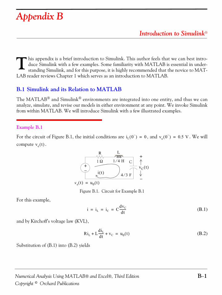
Numerical Analysis Using MATLAB® and Excel®, Third Edition B−1Copyright © Orchard Publications
Appendix B
Introduction to Simulink®
his appendix is a brief introduction to Simulink. This author feels that we can best intro-duce Simulink with a few examples. Some familiarity with MATLAB is essential in under-standing Simulink, and for this purpose, it is highly recommended that the novice to MAT-
LAB reader reviews Chapter 1 which serves as an introduction to MATLAB.
B.1 Simulink and its Relation to MATLAB
The MATLAB® and Simulink® environments are integrated into one entity, and thus we cananalyze, simulate, and revise our models in either environment at any point. We invoke Simulinkfrom within MATLAB. We will introduce Simulink with a few illustrated examples.
Example B.1
For the circuit of Figure B.1, the initial conditions are , and . We willcompute .
Figure B.1. Circuit for Example B.1
For this example,
(B.1)
and by Kirchoff’s voltage law (KVL),
(B.2)
Substitution of (B.1) into (B.2) yields
T
iL 0−( ) 0= vc 0−( ) 0.5 V=
vc t( )
−
+R L
+−
C1 Ω
vs t( ) u0 t( )=
vC t( )i t( )
1 4⁄ H
4 3⁄ F
i iL iC CdvC
dt---------= = =
RiL LdiL
dt------- vC+ + u0 t( )=
Introduction to Simulink®
B−2 Numerical Analysis Using MATLAB® and Excel®, Third EditionCopyright © Orchard Publications
(B.3)
Substituting the values of the circuit constants and rearranging we obtain:
(B.4)
(B.5)
To appreciate Simulink’s capabilities, for comparison, three different methods of obtaining thesolution are presented, and the solution using Simulink follows.
First Method − Assumed Solution
Equation (B.5) is a second−order, non−homogeneous differential equation with constant coeffi-cients, and thus the complete solution will consist of the sum of the forced response and the natu-ral response. It is obvious that the solution of this equation cannot be a constant since the deriva-tives of a constant are zero and thus the equation is not satisfied. Also, the solution cannotcontain sinusoidal functions (sine and cosine) since the derivatives of these are also sinusoids.
However, decaying exponentials of the form where k and a are constants, are possible candi-dates since their derivatives have the same form but alternate in sign.
It can be shown* that if and where and are constants and and are theroots of the characteristic equation of the homogeneous part of the given differential equation,
the natural response is the sum of the terms and . Therefore, the total solution willbe
(B.6)
The values of and are the roots of the characteristic equation
* Please refer to Circuit Analysis II with MATLAB Applications, ISBN 0−9709511−5−9, Appendix B for athorough discussion.
RCdvC
dt--------- LC
d2vC
dt2----------- vC+ + u0 t( )=
13---d2vC
dt2----------- 4
3---dvC
dt--------- vC+ + u0 t( )=
d2vC
dt2----------- 4
dvC
dt--------- 3vC+ + 3u0 t( )=
d2vC
dt2----------- 4
dvC
dt--------- 3vC+ + 3= t 0>
ke at–
k1es1t–
k2es2t–
k1 k2 s1 s2
k1es1t–
k2es2t–
vc t( ) natural response forced response+ vcn t( ) vcf t( )+ k1es1t–
k2es2t–
vcf t( )+ += = =
s1 s2
Numerical Analysis Using MATLAB® and Excel®, Third Edition B−3Copyright © Orchard Publications
Simulink and its Relation to MATLAB
(B.7)
Solution of (B.7) yields of and and with these values (B.6) is written as
(B.8)
The forced component is found from (B.5), i.e.,
(B.9)
Since the right side of (B.9) is a constant, the forced response will also be a constant and wedenote it as . By substitution into (B.9) we obtain
or (B.10)
Substitution of this value into (B.8), yields the total solution as
(B.11)
The constants and will be evaluated from the initial conditions. First, using and evaluating (B.11) at , we obtain
(B.12)
Also,
and
(B.13)
Next, we differentiate (B.11), we evaluate it at , and equate it with (B.13). Thus,
(B.14)
By equating the right sides of (B.13) and (B.14) we obtain
s2 4s 3+ + 0=
s1 1–= s2 3–=
vc t( ) k1e t– k2e 3– t vcf t( )+ +=
vcf t( )
d2vC
dt2----------- 4
dvC
dt--------- 3vC+ + 3= t 0>
vCf k3=
0 0 3k3+ + 3=
vCf k3 1= =
vC t( ) vCn t( ) vCf+= k1e t– k2e 3– t 1+ +=
k1 k2 vC 0( ) 0.5 V=
t 0=
vC 0( ) k1e0 k2e0 1+ + 0.5= =
k1 k2+ 0.5–=
iL iC CdvCdt
---------= = dvCdt
--------- iLC----=,
dvCdt
---------t 0=
iL 0( )C
------------ 0C---- 0= = =
t 0=
dvCdt
---------t 0=
k1– 3k2–=
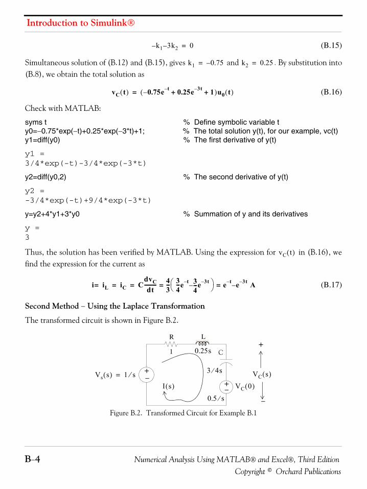
Introduction to Simulink®
B−4 Numerical Analysis Using MATLAB® and Excel®, Third EditionCopyright © Orchard Publications
(B.15)
Simultaneous solution of (B.12) and (B.15), gives and . By substitution into(B.8), we obtain the total solution as
(B.16)
Check with MATLAB:
syms t % Define symbolic variable ty0=−0.75*exp(−t)+0.25*exp(−3*t)+1; % The total solution y(t), for our example, vc(t)y1=diff(y0) % The first derivative of y(t)
y1 =3/4*exp(-t)-3/4*exp(-3*t)
y2=diff(y0,2) % The second derivative of y(t)
y2 =-3/4*exp(-t)+9/4*exp(-3*t)
y=y2+4*y1+3*y0 % Summation of y and its derivatives
y =3
Thus, the solution has been verified by MATLAB. Using the expression for in (B.16), wefind the expression for the current as
(B.17)
Second Method − Using the Laplace Transformation
The transformed circuit is shown in Figure B.2.
Figure B.2. Transformed Circuit for Example B.1
k1– 3k2– 0=
k1 0.75–= k2 0.25=
vC t( ) 0.75– e t– 0.25e 3– t 1+ +( )u0 t( )=
vC t( )
i iL= iC CdvCdt
---------- 43--- 3
4---e t– 3
4---– e 3t–
⎝ ⎠⎛ ⎞ e t– e 3t–– A= == =
−
+R L
+−
C 1
Vs s( ) 1 s⁄= VC s( )I s( )
0.25s
3 4s⁄
+− VC 0( )
0.5 s⁄
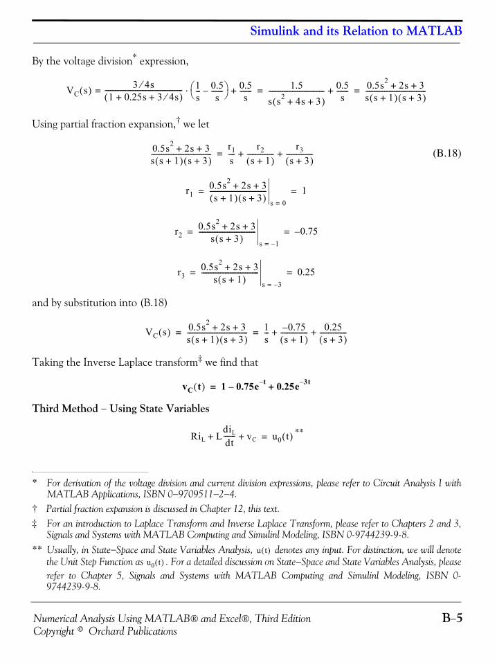
Numerical Analysis Using MATLAB® and Excel®, Third Edition B−5Copyright © Orchard Publications
Simulink and its Relation to MATLAB
By the voltage division* expression,
Using partial fraction expansion,† we let
(B.18)
and by substitution into (B.18)
Taking the Inverse Laplace transform‡ we find that
Third Method − Using State Variables
**
* For derivation of the voltage division and current division expressions, please refer to Circuit Analysis I withMATLAB Applications, ISBN 0−9709511−2−4.
† Partial fraction expansion is discussed in Chapter 12, this text.‡ For an introduction to Laplace Transform and Inverse Laplace Transform, please refer to Chapters 2 and 3,
Signals and Systems with MATLAB Computing and Simulinl Modeling, ISBN 0-9744239-9-8.** Usually, in State−Space and State Variables Analysis, denotes any input. For distinction, we will denote
the Unit Step Function as . For a detailed discussion on State−Space and State Variables Analysis, pleaserefer to Chapter 5, Signals and Systems with MATLAB Computing and Simulinl Modeling, ISBN 0-9744239-9-8.
VC s( ) 3 4s⁄1 0.25s 3 4s⁄+ +( )
---------------------------------------------- 1s--- 0.5
s-------–⎝ ⎠
⎛ ⎞⋅ 0.5s
-------+= 1.5s s2 4s 3+ +( )--------------------------------- 0.5
s-------+ 0.5s2 2s 3+ +
s s 1+( ) s 3+( )------------------------------------= =
0.5s2 2s 3+ +s s 1+( ) s 3+( )------------------------------------
r1s----
r2s 1+( )
----------------r3
s 3+( )----------------+ +=
r10.5s2 2s 3+ +s 1+( ) s 3+( )
----------------------------------s 0=
1= =
r20.5s2 2s 3+ +
s s 3+( )----------------------------------
s 1–=
0.75–= =
r30.5s2 2s 3+ +
s s 1+( )----------------------------------
s 3–=
0.25= =
VC s( ) 0.5s2 2s 3+ +s s 1+( ) s 3+( )------------------------------------ 1
s--- 0.75–
s 1+( )---------------- 0.25
s 3+( )----------------+ += =
vC t( ) 1 0.75e t– 0.25e 3t–+–=
RiL LdiL
dt------- vC+ + u0 t( )=
u t( )u0 t( )
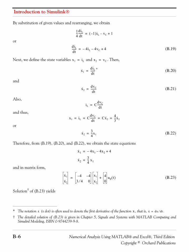
Introduction to Simulink®
B−6 Numerical Analysis Using MATLAB® and Excel®, Third EditionCopyright © Orchard Publications
By substitution of given values and rearranging, we obtain
or
(B.19)
Next, we define the state variables and . Then,
* (B.20)
and
(B.21)
Also,
and thus,
or
(B.22)
Therefore, from (B.19), (B.20), and (B.22), we obtain the state equations
and in matrix form,
(B.23)
Solution† of (B.23) yields
* The notation (x dot) is often used to denote the first derivative of the function , that is, .
† The detailed solution of (B.23) is given in Chapter 5, Signals and Systems with MATLAB Computing andSimulinl Modeling, ISBN 0-9744239-9-8.
14---diL
dt------- 1–( )iL vC– 1+=
diL
dt------- 4iL– 4vC– 4+=
x1 iL= x2 vC=
x· 1diL
dt-------=
x· x x· dx dt⁄=
x· 2dvC
dt---------=
iL CdvC
dt---------=
x1 iL CdvC
dt--------- Cx· 2
43---x· 2= = = =
x· 234---x1=
x· 1 4x1– 4x2– 4+=
x· 234--- x1=
x· 1
x· 2
4– 4–3 4⁄ 0
x1
x2
40
u0 t( )+=
Numerical Analysis Using MATLAB® and Excel®, Third Edition B−7Copyright © Orchard Publications
Simulink and its Relation to MATLAB
Then,
(B.24)
and
(B.25)
Modeling the Differential Equation of Example B.1 with Simulink
To run Simulink, we must first invoke MATLAB. Make sure that Simulink is installed in your sys-tem. In the MATLAB Command prompt, we type:
simulink
Alternately, we can click on the Simulink icon shown in Figure B.3. It appears on the top bar onMATLAB’s Command prompt.
Figure B.3. The Simulink icon
Upon execution of the Simulink command, the Commonly Used Blocks appear as shown in Fig-ure B.4.
In Figure B.4, the left side is referred to as the Tree Pane and displays all Simulink librariesinstalled. The right side is referred to as the Contents Pane and displays the blocks that reside inthe library currently selected in the Tree Pane.
Let us express the differential equation of Example B.1 as
(B.26)
A block diagram representing relation (B.26) above is shown in Figure B.5. We will use Simulinkto draw a similar block diagram.*
* Henceforth, all Simulink block diagrams will be referred to as models.
x1
x2
e t– e– 3t–
1 0.75– e t– 0.25e 3t–+=
x1 iL e t– e– 3t–= =
x2 vC 1 0.75e– t– 0.25e 3t–+= =
d2vC
dt2----------- 4
dvC
dt--------- 3vC 3u0 t( )+––=
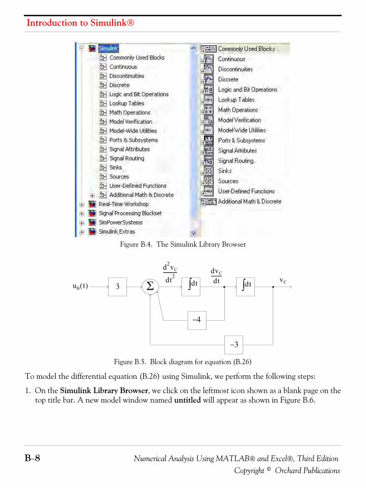
Introduction to Simulink®
B−8 Numerical Analysis Using MATLAB® and Excel®, Third EditionCopyright © Orchard Publications
Figure B.4. The Simulink Library Browser
Figure B.5. Block diagram for equation (B.26)
To model the differential equation (B.26) using Simulink, we perform the following steps:
1. On the Simulink Library Browser, we click on the leftmost icon shown as a blank page on thetop title bar. A new model window named untitled will appear as shown in Figure B.6.
3u0 t( ) Σ dt∫ dt∫
−4
−3
d2vC
dt2----------- dvC
dt--------- vC
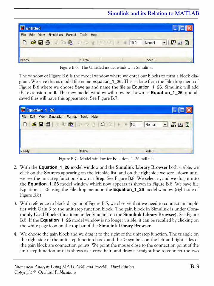
Numerical Analysis Using MATLAB® and Excel®, Third Edition B−9Copyright © Orchard Publications
Simulink and its Relation to MATLAB
Figure B.6. The Untitled model window in Simulink.
The window of Figure B.6 is the model window where we enter our blocks to form a block dia-gram. We save this as model file name Equation_1_26. This is done from the File drop menu ofFigure B.6 where we choose Save as and name the file as Equation_1_26. Simulink will addthe extension .mdl. The new model window will now be shown as Equation_1_26, and allsaved files will have this appearance. See Figure B.7.
Figure B.7. Model window for Equation_1_26.mdl file
2. With the Equation_1_26 model window and the Simulink Library Browser both visible, weclick on the Sources appearing on the left side list, and on the right side we scroll down untilwe see the unit step function shown as Step. See Figure B.8. We select it, and we drag it intothe Equation_1_26 model window which now appears as shown in Figure B.8. We save fileEquation_1_26 using the File drop menu on the Equation_1_26 model window (right side ofFigure B.8).
3. With reference to block diagram of Figure B.5, we observe that we need to connect an ampli-fier with Gain 3 to the unit step function block. The gain block in Simulink is under Com-monly Used Blocks (first item under Simulink on the Simulink Library Browser). See FigureB.8. If the Equation_1_26 model window is no longer visible, it can be recalled by clicking onthe white page icon on the top bar of the Simulink Library Browser.
4. We choose the gain block and we drag it to the right of the unit step function. The triangle onthe right side of the unit step function block and the > symbols on the left and right sides ofthe gain block are connection points. We point the mouse close to the connection point of theunit step function until is shows as a cross hair, and draw a straight line to connect the two
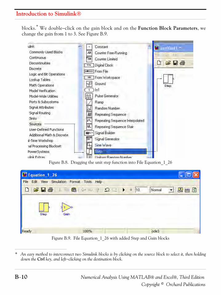
Introduction to Simulink®
B−10 Numerical Analysis Using MATLAB® and Excel®, Third EditionCopyright © Orchard Publications
blocks.* We double−click on the gain block and on the Function Block Parameters, wechange the gain from 1 to 3. See Figure B.9.
Figure B.8. Dragging the unit step function into File Equation_1_26
Figure B.9. File Equation_1_26 with added Step and Gain blocks
* An easy method to interconnect two Simulink blocks is by clicking on the source block to select it, then holdingdown the Ctrl key, and left−clicking on the destination block.
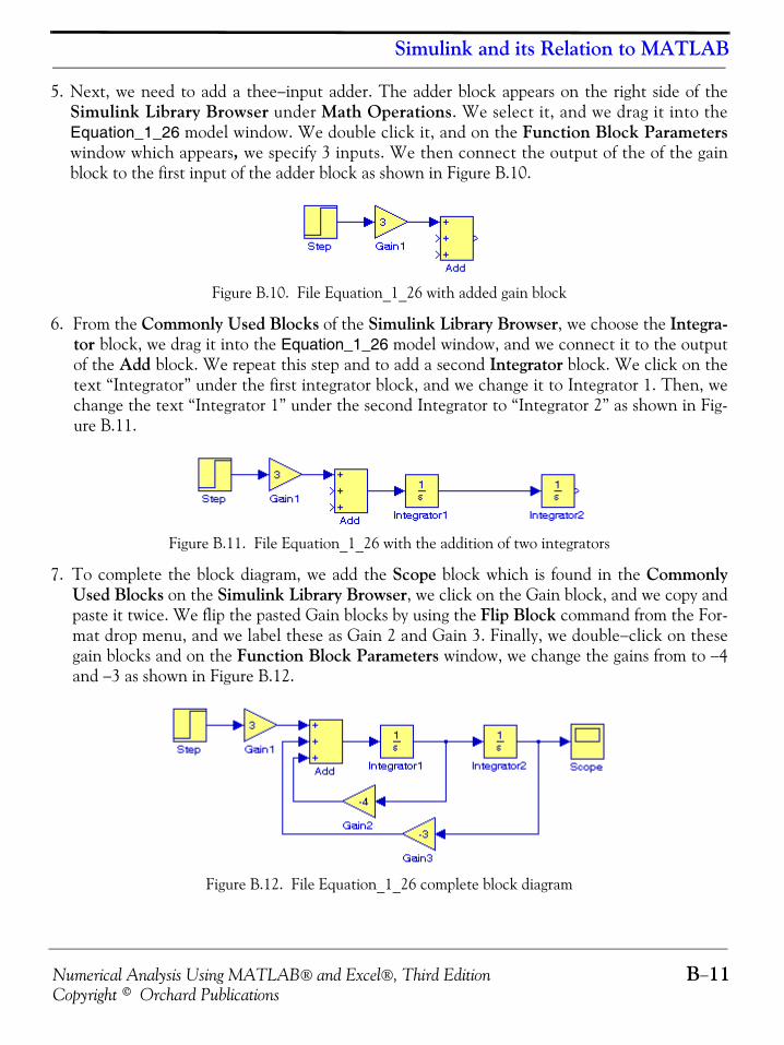
Numerical Analysis Using MATLAB® and Excel®, Third Edition B−11Copyright © Orchard Publications
Simulink and its Relation to MATLAB
5. Next, we need to add a thee−input adder. The adder block appears on the right side of theSimulink Library Browser under Math Operations. We select it, and we drag it into theEquation_1_26 model window. We double click it, and on the Function Block Parameterswindow which appears, we specify 3 inputs. We then connect the output of the of the gainblock to the first input of the adder block as shown in Figure B.10.
Figure B.10. File Equation_1_26 with added gain block
6. From the Commonly Used Blocks of the Simulink Library Browser, we choose the Integra-tor block, we drag it into the Equation_1_26 model window, and we connect it to the outputof the Add block. We repeat this step and to add a second Integrator block. We click on thetext “Integrator” under the first integrator block, and we change it to Integrator 1. Then, wechange the text “Integrator 1” under the second Integrator to “Integrator 2” as shown in Fig-ure B.11.
Figure B.11. File Equation_1_26 with the addition of two integrators
7. To complete the block diagram, we add the Scope block which is found in the CommonlyUsed Blocks on the Simulink Library Browser, we click on the Gain block, and we copy andpaste it twice. We flip the pasted Gain blocks by using the Flip Block command from the For-mat drop menu, and we label these as Gain 2 and Gain 3. Finally, we double−click on thesegain blocks and on the Function Block Parameters window, we change the gains from to −4and −3 as shown in Figure B.12.
Figure B.12. File Equation_1_26 complete block diagram
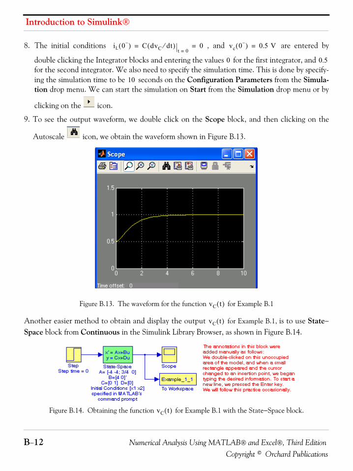
Introduction to Simulink®
B−12 Numerical Analysis Using MATLAB® and Excel®, Third EditionCopyright © Orchard Publications
8. The initial conditions , and are entered by
double clicking the Integrator blocks and entering the values for the first integrator, and for the second integrator. We also need to specify the simulation time. This is done by specify-ing the simulation time to be seconds on the Configuration Parameters from the Simula-tion drop menu. We can start the simulation on Start from the Simulation drop menu or by
clicking on the icon.
9. To see the output waveform, we double click on the Scope block, and then clicking on the
Autoscale icon, we obtain the waveform shown in Figure B.13.
Figure B.13. The waveform for the function for Example B.1
Another easier method to obtain and display the output for Example B.1, is to use State−Space block from Continuous in the Simulink Library Browser, as shown in Figure B.14.
Figure B.14. Obtaining the function for Example B.1 with the State−Space block.
iL 0−( ) C dvC dt⁄( )t 0=
0= = vc 0−( ) 0.5 V=
0 0.5
10
vC t( )
vC t( )
vC t( )
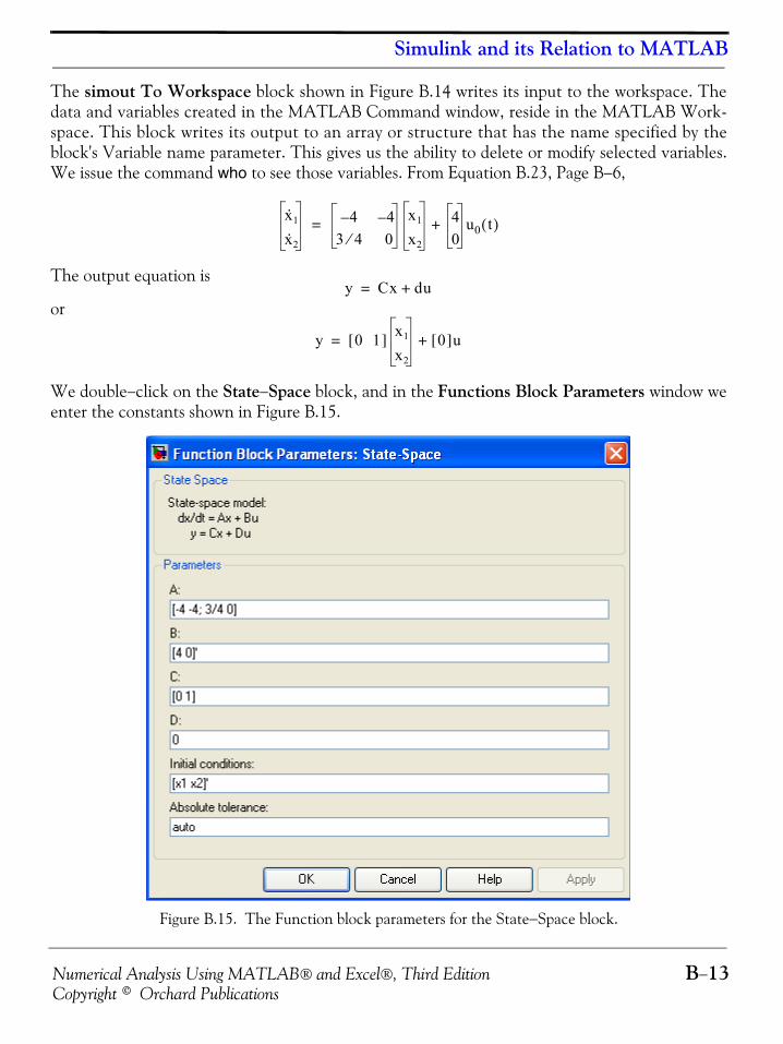
Numerical Analysis Using MATLAB® and Excel®, Third Edition B−13Copyright © Orchard Publications
Simulink and its Relation to MATLAB
The simout To Workspace block shown in Figure B.14 writes its input to the workspace. Thedata and variables created in the MATLAB Command window, reside in the MATLAB Work-space. This block writes its output to an array or structure that has the name specified by theblock's Variable name parameter. This gives us the ability to delete or modify selected variables.We issue the command who to see those variables. From Equation B.23, Page B−6,
The output equation is
or
We double−click on the State−Space block, and in the Functions Block Parameters window weenter the constants shown in Figure B.15.
Figure B.15. The Function block parameters for the State−Space block.
x· 1
x· 2
4– 4–3 4⁄ 0
x1
x2
40
u0 t( )+=
y Cx du+=
y 0 1[ ] x1
x2
0[ ]u+=
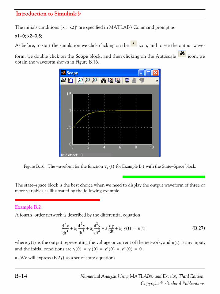
Introduction to Simulink®
B−14 Numerical Analysis Using MATLAB® and Excel®, Third EditionCopyright © Orchard Publications
The initials conditions are specified in MATLAB’s Command prompt as
x1=0; x2=0.5;
As before, to start the simulation we click clicking on the icon, and to see the output wave-
form, we double click on the Scope block, and then clicking on the Autoscale icon, weobtain the waveform shown in Figure B.16.
Figure B.16. The waveform for the function for Example B.1 with the State−Space block.
The state−space block is the best choice when we need to display the output waveform of three ormore variables as illustrated by the following example.
Example B.2 A fourth−order network is described by the differential equation
(B.27)
where is the output representing the voltage or current of the network, and is any input,and the initial conditions are .
a. We will express (B.27) as a set of state equations
x1 x2[ ]'
vC t( )
d 4ydt4--------- a3
d 3ydt3--------- a2
d2ydt2-------- a1
dydt------ a0 y t( )+ + + + u t( )=
y t( ) u t( )y 0( ) y' 0( ) y'' 0( ) y''' 0( ) 0= = = =
Numerical Analysis Using MATLAB® and Excel®, Third Edition B−15Copyright © Orchard Publications
Simulink and its Relation to MATLAB
b. It is known that the solution of the differential equation
(B.28)
subject to the initial conditions , has the solution
(B.29)
In our set of state equations, we will select appropriate values for the coefficients so that the new set of the state equations will represent the differential equa-
tion of (B.28), and using Simulink, we will display the waveform of the output .
1. The differential equation of (B.28) is of fourth−order; therefore, we must define four state vari-ables that will be used with the four first−order state equations.
We denote the state variables as , and , and we relate them to the terms of thegiven differential equation as
(B.30)
We observe that
(B.31)
and in matrix form
(B.32)
In compact form, (B.32) is written as
(B.33)Also, the output is
(B.34)where
d4ydt4-------- 2d2y
dt2-------- y t( )+ + tsin=
y 0( ) y' 0( ) y'' 0( ) y''' 0( ) 0= = = =
y t( ) 0.125 3 t2–( ) 3t tcos–[ ]=
a3 a2 a1 and a0, , ,y t( )
x1 x2 x3, , x4
x1 y t( )= x2dydt------= x3
d 2ydt2---------= x4
d 3ydt3---------=
x· 1 x2=
x· 2 x3=
x· 3 x4=
d 4ydt4--------- x· 4 a0x1– a1x2 a2x3–– a3x4– u t( )+= =
x· 1
x· 2
x· 3
x· 4
0 1 0 00 0 1 00 0 0 1a0– a1– a2– a3–
x1
x2
x3
x4
0001
u t( )+=
x· Ax bu+=
y Cx du+=
Introduction to Simulink®
B−16 Numerical Analysis Using MATLAB® and Excel®, Third EditionCopyright © Orchard Publications
(B.35)
and since the output is defined as
relation (B.34) is expressed as
(B.36)
2. By inspection, the differential equation of (B.27) will be reduced to the differential equation of(B.28) if we let
and thus the differential equation of (B.28) can be expressed in state−space form as
(B.37)
where
(B.38)
Since the output is defined as
in matrix form it is expressed as
x·
x· 1
x· 2
x· 3
x· 4
= A
0 1 0 00 0 1 00 0 0 1a0– a1– a2– a3–
= x
x1
x2
x3
x4
= b
0001
and u,=, , , u t( )=
y t( ) x1=
y 1 0 0 0[ ]
x1
x2
x3
x4
⋅ 0[ ]u t( )+=
a3 0= a2 2= a1 0= a0 1= u t( ) tsin=
x· 1
x· 2
x· 3
x· 4
0 1 0 00 0 1 00 0 0 1a0– 0 2– 0
x1
x2
x3
x4
0001
tsin+=
x·
x· 1
x· 2
x· 3
x· 4
= A
0 1 0 00 0 1 00 0 0 1a0– 0 2– 0
= x
x1
x2
x3
x4
= b
0001
and u,=, , , tsin=
y t( ) x1=
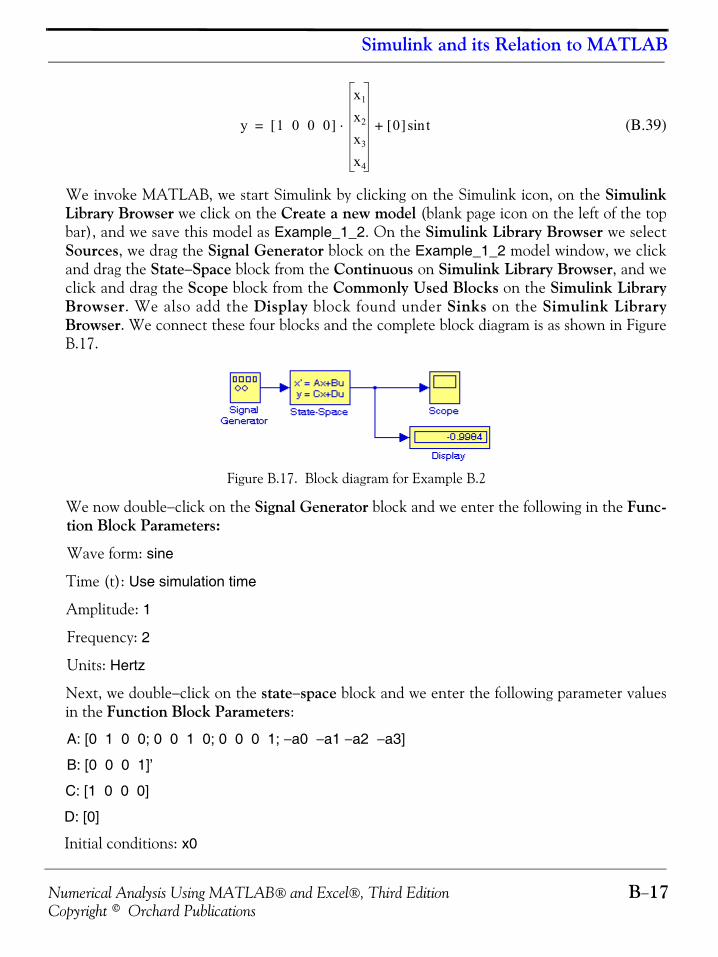
Numerical Analysis Using MATLAB® and Excel®, Third Edition B−17Copyright © Orchard Publications
Simulink and its Relation to MATLAB
(B.39)
We invoke MATLAB, we start Simulink by clicking on the Simulink icon, on the SimulinkLibrary Browser we click on the Create a new model (blank page icon on the left of the topbar), and we save this model as Example_1_2. On the Simulink Library Browser we selectSources, we drag the Signal Generator block on the Example_1_2 model window, we clickand drag the State−Space block from the Continuous on Simulink Library Browser, and weclick and drag the Scope block from the Commonly Used Blocks on the Simulink LibraryBrowser. We also add the Display block found under Sinks on the Simulink LibraryBrowser. We connect these four blocks and the complete block diagram is as shown in FigureB.17.
Figure B.17. Block diagram for Example B.2
We now double−click on the Signal Generator block and we enter the following in the Func-tion Block Parameters:
Wave form: sine
Time (t): Use simulation time
Amplitude: 1
Frequency: 2
Units: Hertz
Next, we double−click on the state−space block and we enter the following parameter valuesin the Function Block Parameters:
A: [0 1 0 0; 0 0 1 0; 0 0 0 1; −a0 −a1 −a2 −a3]
B: [0 0 0 1]’
C: [1 0 0 0]
D: [0]
Initial conditions: x0
y 1 0 0 0[ ]
x1
x2
x3
x4
⋅ 0[ ] tsin+=
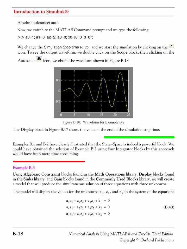
Introduction to Simulink®
B−18 Numerical Analysis Using MATLAB® and Excel®, Third EditionCopyright © Orchard Publications
Absolute tolerance: auto
Now, we switch to the MATLAB Command prompt and we type the following:
>> a0=1; a1=0; a2=2; a3=0; x0=[0 0 0 0]’;
We change the Simulation Stop time to , and we start the simulation by clicking on the icon. To see the output waveform, we double click on the Scope block, then clicking on the
Autoscale icon, we obtain the waveform shown in Figure B.18.
Figure B.18. Waveform for Example B.2
The Display block in Figure B.17 shows the value at the end of the simulation stop time.
Examples B.1 and B.2 have clearly illustrated that the State−Space is indeed a powerful block. Wecould have obtained the solution of Example B.2 using four Integrator blocks by this approachwould have been more time consuming.
Example B.3 Using Algebraic Constraint blocks found in the Math Operations library, Display blocks foundin the Sinks library, and Gain blocks found in the Commonly Used Blocks library, we will createa model that will produce the simultaneous solution of three equations with three unknowns.
The model will display the values for the unknowns , , and in the system of the equations
(B.40)
25
z1 z2 z3
a1z1 a2z2 a3z3 k1+ + + 0=
a4z1 a5z2 a6z3 k2+ + + 0=
a7z1 a8z2 a9z3 k3+ + + 0=
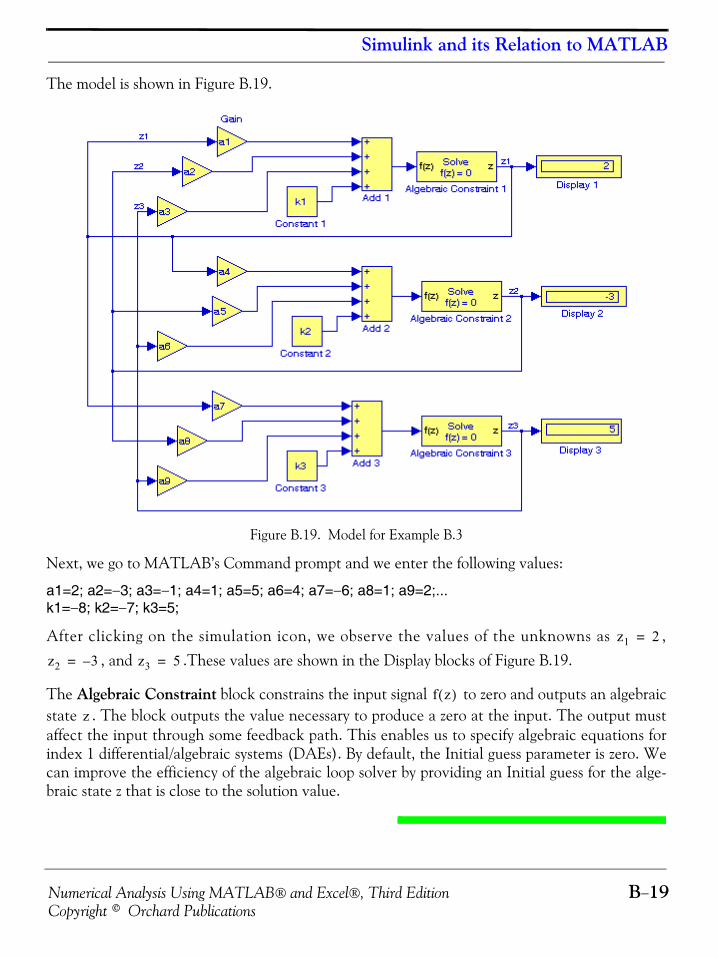
Numerical Analysis Using MATLAB® and Excel®, Third Edition B−19Copyright © Orchard Publications
Simulink and its Relation to MATLAB
The model is shown in Figure B.19.
Figure B.19. Model for Example B.3
Next, we go to MATLAB’s Command prompt and we enter the following values:
a1=2; a2=−3; a3=−1; a4=1; a5=5; a6=4; a7=−6; a8=1; a9=2;...k1=−8; k2=−7; k3=5;
After clicking on the simulation icon, we observe the values of the unknowns as ,, and .These values are shown in the Display blocks of Figure B.19.
The Algebraic Constraint block constrains the input signal to zero and outputs an algebraicstate . The block outputs the value necessary to produce a zero at the input. The output mustaffect the input through some feedback path. This enables us to specify algebraic equations forindex 1 differential/algebraic systems (DAEs). By default, the Initial guess parameter is zero. Wecan improve the efficiency of the algebraic loop solver by providing an Initial guess for the alge-braic state z that is close to the solution value.
z1 2=
z2 3–= z3 5=
f z( )z
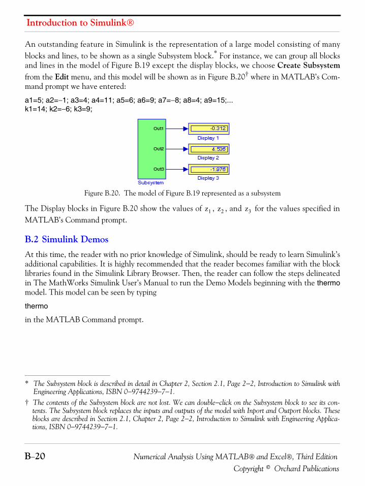
Introduction to Simulink®
B−20 Numerical Analysis Using MATLAB® and Excel®, Third EditionCopyright © Orchard Publications
An outstanding feature in Simulink is the representation of a large model consisting of manyblocks and lines, to be shown as a single Subsystem block.* For instance, we can group all blocksand lines in the model of Figure B.19 except the display blocks, we choose Create Subsystemfrom the Edit menu, and this model will be shown as in Figure B.20† where in MATLAB’s Com-mand prompt we have entered:
a1=5; a2=−1; a3=4; a4=11; a5=6; a6=9; a7=−8; a8=4; a9=15;...k1=14; k2=−6; k3=9;
Figure B.20. The model of Figure B.19 represented as a subsystem
The Display blocks in Figure B.20 show the values of , , and for the values specified inMATLAB’s Command prompt.
B.2 Simulink DemosAt this time, the reader with no prior knowledge of Simulink, should be ready to learn Simulink’sadditional capabilities. It is highly recommended that the reader becomes familiar with the blocklibraries found in the Simulink Library Browser. Then, the reader can follow the steps delineatedin The MathWorks Simulink User’s Manual to run the Demo Models beginning with the thermomodel. This model can be seen by typing
thermo
in the MATLAB Command prompt.
* The Subsystem block is described in detail in Chapter 2, Section 2.1, Page 2−2, Introduction to Simulink withEngineering Applications, ISBN 0−9744239−7−1.
† The contents of the Subsystem block are not lost. We can double−click on the Subsystem block to see its con-tents. The Subsystem block replaces the inputs and outputs of the model with Inport and Outport blocks. Theseblocks are described in Section 2.1, Chapter 2, Page 2−2, Introduction to Simulink with Engineering Applica-tions, ISBN 0−9744239−7−1.
z1 z2 z3
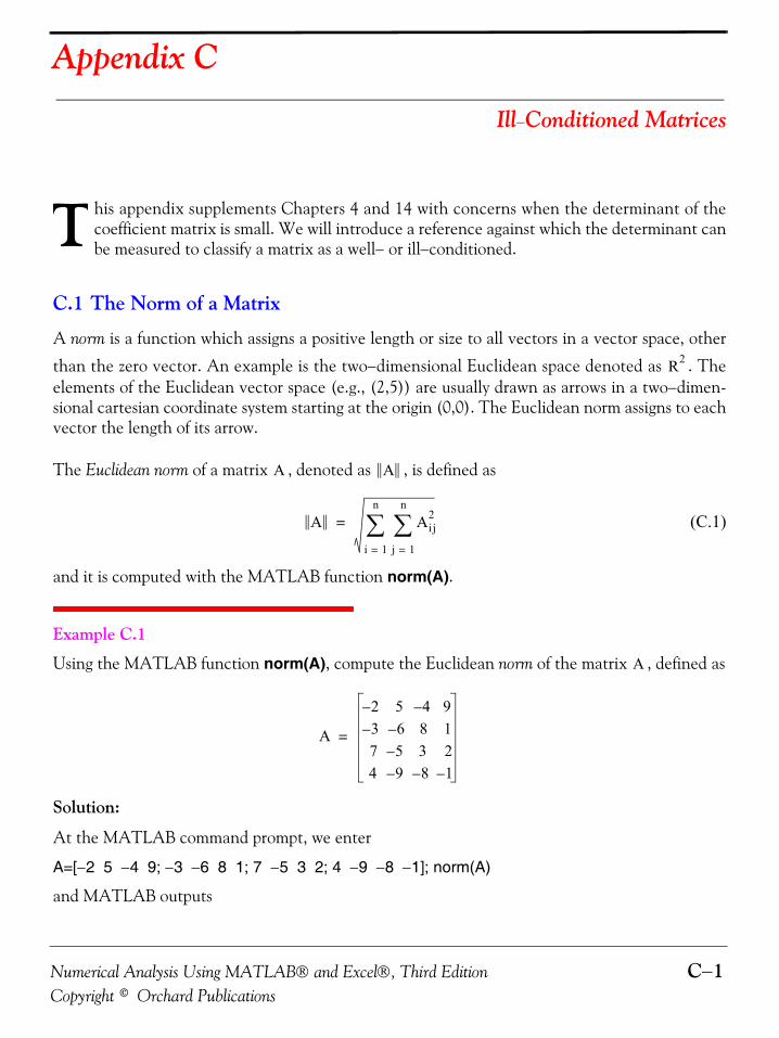
Numerical Analysis Using MATLAB® and Excel®, Third Edition C−1Copyright © Orchard Publications
Appendix C
Ill−Conditioned Matrices
his appendix supplements Chapters 4 and 14 with concerns when the determinant of thecoefficient matrix is small. We will introduce a reference against which the determinant canbe measured to classify a matrix as a well− or ill−conditioned.
C.1 The Norm of a Matrix
A norm is a function which assigns a positive length or size to all vectors in a vector space, other
than the zero vector. An example is the two−dimensional Euclidean space denoted as . Theelements of the Euclidean vector space (e.g., (2,5)) are usually drawn as arrows in a two−dimen-sional cartesian coordinate system starting at the origin (0,0). The Euclidean norm assigns to eachvector the length of its arrow.
The Euclidean norm of a matrix , denoted as , is defined as
(C.1)
and it is computed with the MATLAB function norm(A).
Example C.1
Using the MATLAB function norm(A), compute the Euclidean norm of the matrix , defined as
Solution:
At the MATLAB command prompt, we enter
A=[−2 5 −4 9; −3 −6 8 1; 7 −5 3 2; 4 −9 −8 −1]; norm(A)
and MATLAB outputs
T
R2
A A
A Aij2
j 1=
n
∑i 1=
n
∑=
A
A
2– 5 4– 93– 6– 8 17 5– 3 24 9– 8– 1–
=
Appendix C Ill−Conditioned Matrices
C−2 Numerical Analysis Using MATLAB® and Excel®, Third EditionCopyright © Orchard Publications
ans = 14.5539
C.2 Condition Number of a Matrix
The condition number of a matrix is defined as
(C.2)
where is the norm of the matrix defined in relation (C.1) above. Matrices with conditionnumber close to unity are said to be well−conditioned matrices, and those with very large conditionnumber are said to be ill−conditioned matrices.
The condition number of a matrix is computed with the MATLAB function cond(A).
Example C.2
Using the MATLAB function cond(A), compute the condition number of the matrix definedas
Solution:
At the MATLAB command prompt, we enter
A=[−2 5 −4 9; −3 −6 8 1; 7 −5 3 2; 4 −9 −8 −1]; cond(A)
and MATLAB outputs
ans = 2.3724
This condition number is relatively close to unity and thus we classify matrix A as a well-condi-tioned matrix.
We recall from Chapter 4 that if the determinant of a square matrix A is singular, that is, if, the inverse of A is undefined. Please refer to Chapter 4, Page 4−22.
A
k A( ) A A 1–⋅=
A A
A
A
A
2– 5 4– 93– 6– 8 17 5– 3 24 9– 8– 1–
=
det A( ) 0=
Numerical Analysis Using MATLAB® and Excel®, Third Edition C−3Copyright © Orchard Publications
Hilbert Matrices
Now, let us consider that the coefficient matrix* is very small, i.e., almost singular. Accordingly,we classify such a matrix as ill−conditioned.
C.3 Hilbert Matrices
Let be a positive integer. A unit fraction is the reciprocal of this integer, that is, . Thus, are unit fractions. A Hilbert matrix is a matrix with unit fraction elements
(C.3)
Shown below is an example of the Hilbert matrix.
(C.4)
* In general, a system with m linear equations and n unknowns can be written as
where are the unknowns and the numbers are the coefficients of the system.
The coefficient matrix is the matrix with the coefficient as the (i,j)-th entry:
a11x1 a12x2 …+a1nxn+ + b1=
a21x1 a22x2 …+a2nxn+ + b2=
... ... ... ... ...am1x1 am2x2 …+amnxn+ + bm=
x1 x2 … xn, , , a11 a12 … amn, , ,
m n× aij
a11 a12 … a1n
a21 a22 … a2n
… … … …am1 am1 am1 am1
n 1 n⁄1 1 1 2⁄,⁄ 1 3⁄ …, ,
Bij 1 i j 1–+( )⁄=
5 5×
11--- 1
2--- 1
3--- 1
4--- 1
5---
12--- 1
3--- 1
4--- 1
5--- 1
6---
13--- 1
4--- 1
5--- 1
6--- 1
7---
14--- 1
5--- 1
6--- 1
7--- 1
8---
15--- 1
6--- 1
7--- 1
8--- 1
9---
Appendix C Ill−Conditioned Matrices
C−4 Numerical Analysis Using MATLAB® and Excel®, Third EditionCopyright © Orchard Publications
MATLAB’s function hilb(n) displays the Hilbert matrix.
Example C.3
Compute the determinant and the condition number of the Hilbert matrix using MATLAB.
Solution:
At the MATLAB command prompt, we enter
det(hilb(6))
and MATLAB outputs
ans =
5.3673e-018
This is indeed a very small number and for all practical purposes this matrix is singular.
We can find the condition number of a matrix A with the cond(A) MATLAB function. Thus, forthe Hilbert matrix,
cond(hilb(6))
ans = 1.4951e+007
This is a large number and if the coefficient matrix is multiplied by this number, seven decimalplaces might be lost.
Let us consider another example.
Example C.4
Let where and
Compute the values of the vector .
Solution:
Here, we are asked to find the values of and of the linear system
n n×
6 6×
6 6×
Ax b= A 0.585 0.3790.728 0.464
= b 0.1870.256
=
x
x1 x2
0.585 0.3790.728 0.464
x1
x2
⋅ 0.1870.256
=
Numerical Analysis Using MATLAB® and Excel®, Third Edition C−5Copyright © Orchard Publications
Hilbert Matrices
Using MATLAB, we define and , and we use the left division operation, i.e.,
A=[0.585 0.378; 0.728 0.464]; b=[0.187 0.256]'; x=b\A
x = 2.9428 1.8852
Check:
A=[0.585 0.378; 0.728 0.464]; x=[2.9428 1.8852]'; b=A*x
b = 2.4341 3.0171
but these are not the given values of the vector , so let us check the determinant and the condi-tion number of the matrix .
determinant = det(A)
determinant = -0.0037
condition=cond(A)
condition = 328.6265
Therefore, we conclude that this system of equations is ill-conditioned and the solution is invalid.
Example C.4 above should serve as a reminder that when we solve systems of equations usingmatrices, we should check the determinants and the condition number to predict possible floatingpoint and roundoff errors.
A b
bA
References and Suggestions for Further StudyA. The following publications by The MathWorks, are highly recommended for further study. They
are available from The MathWorks, 3 Apple Hill Drive, Natick, MA, 01760, www.mathworks.com.
1. Getting Started with MATLAB
2. Using MATLAB
3. Using MATLAB Graphics
4. Financial Toolbox
5. Statistics Toolbox
B. Other references indicated in footnotes throughout this text, are listed below.
1. Mathematics for Business, Science, and Technology with MATLAB and Excel Computations, ThirdEdition, ISBN-13: 978−1−934404−01−2
2. Circuit Analysis I with MATLAB Applications, ISBN 0−9709511−2−4
3. Circuit Analysis II with MATLAB Applications, ISBN 0−9709511−5−9
4. Introduction to Simulink with Engineering Applications, ISBN 0-9744239-7-1
5. Signals and Systems with MATLAB Computing and Simulink Modeling, Third Edition, ISBN 0-9744239-9-8
6. Handbook of Mathematical Functions, ISBN 0-4866127-2-4
7. CRC Standard Mathematical Tables, ISBN 0-8493-0626-4
IndexSymbols Chebyshev polynomials of the disp(x) MATLAB function 2-5% (percent) symbol 1-2 second kind 15-22 Display block in Simulink B-18%d MATLAB symbol 2-5 Cholesky factorization 14-23 display formats in MATLAB 1-31%e MATLAB symbol 2-21 classification of differential equations 5-2 distinct poles 12-2%s MATLAB symbol 2-21 clc MATLAB command 1-2 distinct roots of characteristic%u MATLAB symbol 2-21 clear MATLAB command 1-2 equation 5-9
coefficient matrix - see matrix divided differences 7-1A cofactors - see matrix division of complex numbers 3-13
collect(s) MATLAB function 7-15, 12-11 dot division operator in MATLAB 1-21abs(z) MATLAB function 1-24 column vector 1-19 dot exponentation operatorabsolute cell in Excel 2-19 command screen in MATLAB 1-1 in MATLAB 1-21absolutely convergent 15-10 command window in MATLAB 1-1 dot multiplication operatorAdams’ method 9-13 commas in MATLAB 1-7 in MATLAB 1-21Add Trendline Excel feature 8-6 comment line in MATLAB 1-2 dsolve(s) MATLAB function 9-5adjoint of a matrix - see matrix Commonly Used Blocks in Simulink B-7 dynamic programming 16-4algebraic constrain block in Simulink B-18 complementary solution A-1algebraic form of the Legendre complex conjugate 1-4 E polynomials 15-17 complex numbers 1-2, 3-11alternate form of the trigonometric complex poles 12-5 Editor window in MATLAB 1-1, 1-27 Fourier series 6-25 complex roots of characteristic Editor/Debugger in MATLAB 1-1, 1-2alternating current 3-1 equation 5-9 eigenvalues 5-30angle(z) MATLAB function 1-24 cond(A) MATLAB function C-2 eigenvectors 5-39angular velocity 3-2 condition number of a matrix - see matrix element-by-element divisionantidifference 7-12 configuration parameters in Simulink B-12 in MATLAB 1-21approximations with Excel 2-7 congugate of a matrix - see matrix element-by-element exponentiationassociated Legendre differential conj(A) MATLAB function 4-8 in MATLAB 1-21 equation 15-18 conj(x) MATLAB function 4-8 element-by-element multiplicationassociated Legendre functions of the conjugate of a complex number 3-12 in MATLAB 1-19, 1-21 first and second kind 15-18 connected network 16-15 elements of a matrix - see matrixAutoFill Excel feature 2-9, 2-15 constraints in linear programming 16-1 eps in MATLAB 1-22, 1-27autoscale icon in Simulink B-12 Contents Pane in Simulink B-7 equating the numerators procedureaxis MATLAB command 1-17, 1-22 conv(a,b) MATLAB function 1-6 in partial fraction expansion 12-13
Cramer’s rule 4-18, 8-4 Erlang distribution 13-16B cubic interpolarion in MATLAB 7-25 error function 10-4
cubic spline interpolarion in MATLAB 7-25 error in method of least squares 8-3backward substitution. 14-10 curve fitting 8-1 Euclidean norm C-1Bessel function of negative order n 15-2 curved regression 8-7, 8-14 Euler’s identities 3-14Bessel function of n 15-1 cycle 3-2 even functions 6-7, 6-31Bessel functions 15-1 cyclic frequency 3-3 even symmetry 6-7Bessel functions of the first kind 15-7 exit MATLAB command 2, 33Bessel functions of the second kind 15-7 D EXP(GAMMALN(n)) Excel function 13-5besselj(n,x) MATLAB function 15-3 expand(s) MATLAB function 7-13, 12-9BESSELJ(x,n) Excel function 15-3 Data Analysis Toolpack in Excel 8-7 exponential form of complexbeta distribution 13-20 data points in MATLAB 1-14 numbers 3-14beta function 13-17 decibel 12 exponential form of thebeta(m,n) MATLAB function 13-19 decimal format 2-21 Fourier series 6-29BETADIST Excel function 13-21 deconv(p,q) MATLAB function 1-6, 7-8 eye(n) MATLAB function 4-6, 14-24bisection method for root default color in MATLAB 1-14 eye(size(A)) MATLAB function 4-7 approximation 2-19 default line in MATLAB 1-15box MATLAB command 1-12 default marker in MATLAB 1-14 F
default values in MATLAB 1-11C degree of differential equation 5-3 factor(p) MATLAB function 12-3
demo in MATLAB 1-2 factorial polynomials 7-6Casorati’s determinant 11-2 determinant - see matrix Fibonacci numbers 11-7Cayley-Hamilton theorem 5-30 diag(v,k) MATLAB function 14-24 figure window in MATLAB 1-14characteristic (auxiliary) equation 5-8 diagonal elements of a matrix - see matrix finite differences 7-1characteristic equation of a second diagonal of a matrix - see matrix first divided difference 7-1 order difference equation 11-3 diff(s) MATLAB function 2-6 first harmonic 6-1chart type in Excel 2-10 difference equations A-1 fixed point format 2-21Chart Wizard Excel feature 2-10, 8-6 difference operator 7-4, 11-1 Flip Block command in Simulink B-11Chebyshev polynomials 15-22 differences - see finite differences forced response 5-8Chebyshev polynomials of the dipole 15-12 forcing function A-1 first kind 15-22 direct terms in MATLAB 12-1 format MATLAB command 1-31
directed network 16-15 format specifiers in MATLAB 2-21
IN1
forward substitution 14-10 improper integral 13-1 Math Operations Library in Simulink B-11Fourier analysis 3-2 improper rational function 12-1 MATLAB Demos 1-2Fourier series 6-1 increments between points matrix (matrices) 4-1fplot MATLAB command 1-27 in MATLAB 1-14 adjoint of 4-22fprintf MATLAB command 7-29 in-phase sinusoids 3-3 coefficient C-3frequency 3-2 input(‘string’) MATLAB command 2-2 cofactors of 4-11Frequency Modulation (FM) 15-4 int(f,a,b) MATLAB function 10-5 condition number of C-2frequency response 1-11 interp1(x,y,xi) MATLAB function 7-24 conformable for addition 4-2full-wave rectifier with even interp1(x,y,xi,’method’) MATLAB conformable for multiplication 4-4 symmetry 6-24 function 7-25 conformable for subtraction 4-2function block parameters in Simulink B-10 interp2(x,y,z,xi,yi) MATLAB congugate of 4-8function files in MATLAB 1-26, 1-27, 2-4 function 7-25 determinant of 4-9fundamental frequency 6-1 interp2(x,y,z,xi,yi,’method’) MATLAB diagonal elements of 4-1fundamental theorem of function 7-25 diagonal of 4-6 integral calculus 7-12 interpolation 7-1 elements of 4-1fundamental theorem of interpolation with MATLAB 7-24 Hermitian 4-9 sum calculus 7-13 interval halving 2-19 Hilbert C-3fzero MATLAB function 1-27, 1-29 inverse of a matrix - see matrix identity 4-6fzero(‘function’,x0) MATLAB isoprofit line 16-2 ill-conditioned 4-22, C-2 function 12-18 inverse of 4-23fzero(f,x) MATLAB function 2-7 J lower triangular 4-6
main diagonal elements of 4-1G j operator 3-11 main diagonal of 4-1
minor of determinant 4-13Gain block in Simulink B-18 L non-singular 4-22gamma distribution 13-16 scalar 4-6gamma function 13-1 L’ Hôpital’s rule 13-2 singular 4-22gamma(n) MATLAB function 13-3, 13-10 lagging sinudoid 3-3 size of 4-7GAMMADIST Excel function 13-16 Lagrange’s interpolation method 7-17 skew-Hermitian 4-9GAMMALN Excel function 13-5 Laguerre polynomials 15-21 skew-symmetric 4-8Gaussian elimination method 4-20, 14-9 leading sinusoid 3-3 square 4-1Genenbauer 15-22 least squares 8-2, 8-3 symmetric 4-8general solution of a differential least squares line 8-2 trace of 4-2 equation 5-6 least-squares curve 8-2 transpose of 4-7generalized factorial function 13-1 least-squares parabola 8-2, 8-7 unitary 14-25generating function for Bessel functions Legendre functions 15-10 upper triangular 4-5 of the first kind of integer order 15-9 Legendre functions of the well-conditioned C-2generating function for Legendre second kind 15-11 zero matrix - see matrix polynomials 15-12 Legendre polynomials 15-11 matrix left division in MATLAB 4-26Goal Seek Excel feature 2-16 Legendre polynomials in matrix multiplication in MATLAB 1-19, 1-20Gram-Schmidt orthogonalization trigonometric form 15-18 mesh(x,y,z) MATLAB command 1-17 procedure 5-39, 14-7 legendre(n,x) MATLAB function 15-19 mesh(Z) MATLAB function 7-32Gregory-Newton Backward Legendre’s equation 15-10 meshgrid(x,y) MATLAB command 1-17 Interpolation Formula 7-21 lims = MATLAB function 1-27 method of Frobenius 15-1Gregory-Newton Forward line graph 16-4 method of least squares 8-2, 8-3 Interpolation Formula 7-19 line spectrum 6-33 method of Picard 15-1grid MATLAB command 1-11 linear factor 1-9 method of undeterminedgtext MATLAB command 1-14, 15-25 linear interpolarion 7-25 coefficients 5-10, 11-2, A-1
linear programming 16-1 method of variation of parameters 5-20H linear regression 8-2 m-file in MATLAB 1-1 1-26, 1-27
linspace MATLAB command 1-14 Milne’s method 9-15half-wave rectifier 6-19, 6-22 ln (natural logarithm) 1-12 minimum span problems 16-15half-wave symmetry 6-7, 6-31 log (common logarithm) 1-12 minor of determinant - see matrixhelp in MATLAB 1-2, 1-15 log(x) MATLAB function 1-12 MINVERSE Excel function 4-28Hermitian matrix - see matrix log10(x) MATLAB function 1-12 MMULT Excel function 4-28, 4-29hilb(n) MATLAB function C-4 log2(x) MATLAB function 1-12 modified Bessel functions 15-7Hilbert matrix - see matrix loglog MATLAB command 1-12, 34 modulation index 15-4homogeneous difference equation 11-2 lower triangular matrix - see matrix multiple poles 12-6Hz (Hertz) 3-3 lsqnonneg MATLAB function 14-28 multiplication of complex numbers 3-12
LU factorization method 14-9I lu(A) MATLAB function 14-12, 14-14 N
identity matrix - see matrix M NaN in MATLAB 1-27ill-conditioned matrix - see matrix natural response 5-8, A-1imag(z) MATLAB function 1-24 Maclaurin power series 6-41, 7-6 nearest neighbor interpolarion 7-25imaginary axis 3-10 main diagonal elements - see matrix network analysis 16-14imaginary number 3-10 main diagonal of a matrix - see matrix Neumann functions 15-7
IN2
Newton’s divided difference quadratic factor 1-9 Stirling’s asymptotic series interpolation method 7-15 quit MATLAB command 1-2 for the G(n) function 13-9Newton-Cotes 8-panel rule 10-10 string in MATLAB 1-17non-homogeneous difference R subplot MATLAB command 1-18 equation 11-2 surface zonal harmonics 15-11non-homogeneous ODE 5-6 radian frequency 3-2 svd(A) MATLAB function 14-28non-singular matrix - see matrix rational polynomial 1-8 sym, syms MATLAB symbolicnorm C-1 rationalization of the quotient 3-13 expressions 12-4norm(A) MATLAB function C-1 real axis 3-10 symbolic expressions in MATLAB 12-3numeric expressions in MATLAB 12-4 real number 3-11 Symbolic Math Toolbox in MATLAB 12-4numerical evaluation of Fourier real(z) MATLAB function 1-24 symmetric matrix - see matrix coefficients 6-36 recursion A-1 symmetry 6-7, 6-14, 6-31
recursive method A-1O regression 8-1 T
regression analysis 8-7odd functions 6-8, 6-31 relative cell in Excel 2-19 Taylor series 5-24, 6-41, 6-44odd symmetry 6-7 repeated poles 5-9, 12- 6 Taylor series expansion method 9-1ODE (Ordinary Differential Equation) 5-3 residue(r,p,k) MATLAB function 12-1 text MATLAB command 1-14, 1-17ode23 MATLAB function 9-9 revolutions per second 3-5 third harmonic 6-1ode45 MATLAB function 9-9 Rodrigues’ formula 15-12, 15-18 title(‘string’) in MATLAB 1-12one-dimensional wave equation 5-3 roots of polynomials 1-3 trace of a matrix - see matrixoptimum path policy 16-5 roots(p) MATLAB function 1-3, 1-8 transpose of a matrix - see matrixorder of a differential equation 5-3 rotating vector 3-5 trapezoidal rule 10-1ordinary differential equation 5-3 round(n) MATLAB function 1-24 trapz(x,y) MATLAB function 10-3, 10-5oriented network 16-15 row vector 1-3, 1-19 Tree Pane in Simulink B-7orthogonal basis 14-5 Runge-Kutta method 5-24, 9-5 Trendline Excel feature 8-9orthogonal functions 6-2, 14-1, 14-2 triangular waveform 6-11, 6-19orthogonal system 15-9 S trigonometric Fourier series 6-1orthogonal trajectories 14-2 trigonometric relations 3-5orthogonal unit vectors 14-5 sawtooth waveform 6-10, 6-18 two-dimensional plots 7-32orthogonal vectors 5-39, 14-4 scalar matrix - see matrix type of a diferential equation 5-2orthonormal basis 14-5 Scope block in Simulink B-12out-of-phase sinusoids 3-3 script file in MATLAB 1-26 Uoverdetermined system 8-3 second divided difference 7-1
second harmonic 6-1 ultraspherical functions 15-22P semicolons in MATLAB 1-7 undetermined system 8-3
semilogx MATLAB command 1-12 unit fraction C-3parabolic curve 8-1 semilogy MATLAB command 1-12 unitary matrix - see matrixpartial differential equation (PDE) 5-3 simple differential equations 5-1 upper triangular matrix - see matrixpartial fraction expansion 12-1 simplex method 16-4PDE (Partial Differential Equation) 5-3 Simpson’s rule 10-6 VPearson correlation coefficient 8-10 Simulation drop menu in Simulink B-12period 3-2, 3-3 simulation start icon in Simulink B-12 VLOOKUP Excel function 7-23periodic waveform 3-2 Simulink icon B-7phasor 3-2 Simulink Library Browser B-8 Wplot area in Excel 6 singular matrix - see matrixplot MATLAB command 1-9, 1-12, 1-15 Singular Value Decomposition 14-28 Wallis’s formulas 13-16plot3 MATLAB command 1-16 Sinks library B-18 Weber functions 15-7polar form of complex numbers 3-15 sinusoids 3-2 well-conditioned matrix - see matrixpolar plot in MATLAB 1-24 size of a matrix - see matrix while end in MATLAB 2-4polar(theta,r) MATLAB function 1-24 skew-Hermitian matrix - see matrix Wronskian determinant 5-10, 11-2poles 12-2 skew-symmetric matrix - see matrixpoly MATLAB function 1-4 solution of the homogeneous ODE 5-8 Xpolyder MATLAB function 1-7 solutions of ODEs 5-6polyfit(x,y,n) MATLAB function 8-11 space equations 5-24 xlabel MATLAB command 1-12polynomial construction from known spectrum analyzer 33 XY (Scatter) in Excel 8-6 roots in MATLAB 1-4 spherical harmonics 15-18polyval(p,x) MATLAB function 1-5, 8-11 sprintf MATLAB command 2-5 Ypower series 6-40 sqrt MATLAB function 10-12proper rational function 12-1 square matrix - see matrix ylabel MATLAB command 1-12
square waveformQ 6-9, 6-14, 6-16, 6-48, 6-49 Z
start simulation in Simulink B-12QR factorization 14-25 state equations 5-24 zero matrix - see matrixqr(A) MATLAB function 14-25 state transition matrix 5-28 zeros 12-2quad MATLAB function 10-10 state variables 5-24 zlabel MATLAB command 1-17quad8 MATLAB function 10-10 State-Space block in Simulink B-12quadratic curve 8-1
IN3