Numerical and laboratory attoclock simulations on noble gas atoms

Vladislav V. Serov,1 Joshua Cesca,2 and Anatoli S. Kheifets2

1 Department of Theoretical Physics, Saratov State University, 83 Astrakhanskaya, Saratov 410012, Russia2Research School of Physics, The Australian National University, Canberra ACT 0200, Australia

(Dated: December 8, 2020)

We conduct a systematic theoretical modeling of strong field tunneling ionization of noble gasatoms, from He to Xe, by elliptically polarized laser pulses in the so-called attoclock setup. Ourtheoretical model is based on a numerical solution of the time-dependent Schrodinger equation inthe single active electron approximation. We simulate laboratory measurements utilizing few opticalcycle pulses to benchmark our calculations against experiment. We further conduct “numericalattoclock” simulations with short, nearly single-cycle pulses and to test various tunneling ionizationmodels. We examine the attoclock offset angles as affected by the target orbital structure and thelaser pulse intensity. Finally, we exclude a finite tunneling time scenario and attribute the attoclockoffset angle entirely to the Coulomb field of the ion remainder as was recently demonstrated for thehydrogen atom [U. S. Sainadh et al Nature 568, 75 (2019)].

PACS numbers: 32.80.Rm, 32.80.Fb, 42.50.Hz

I. INTRODUCTION

Tunneling ionization of noble gas atoms by circularlyor elliptically polarized laser pulses has been studied ac-tively over the past decade. It had been suggested [1]that the photoelectron momentum distribution (PMD)following such an ionization process can be used for map-ping orbital structure of the target. The use of circularlypolarized light rather than linear polarization minimizesre-scattering and inter-cycle interference to produce atwo dimensional PMD images with a clear signature ofthe angular orbital structure [2]. Electron momentumimaging with circular or elliptical light can also be em-ployed for testing various tunneling ionization scenarios[3, 4]. Another major usage of PMD with elliptically po-larized light is the so-called attoclock aiming to resolvethe tunneling time that photoelectron spends under thebarrier [5–7]. “Improved” attoclocks driven by two laserpulses (double-handed attoclocks) have also been pro-posed [8, 9]. Results of earlier and more recent measure-ments of tunneling time in noble gas atoms [10–12] are asubject of the continuing debate [13, 14]. Meanwhile, thecleanest attoclock measurement on the atomic hydrogenhas effectively eliminated a finite tunneling time scenario[15]. Another interesting effect discovered in tunnelingionization of noble gas atoms with circular light is itsstrong dependence on the magnetic projection quantumnumber [16]. It appears that ionization with a light wavecounter-rotating with the electron cloud has a strongpropensity over the co-rotating one. This effect can beused to produce nearly complete spin polarization of thephotoelectron beam [17, 18]. Such a strong angular mo-mentum dependence can also be observed in the Wignertime delay [19] and the attoclock offset angles [20–22].

Despite this rich physics that can be probed by atto-clock experiments on noble gas atoms, only very few mea-surements have been reported to date on heavier atomsbeyond helium [7, 9, 12]. This makes a strong case for asystematic attoclock investigation across a series of tar-get atoms in a wide range of field intensities. Such in-vestigation is currently underway [23]. To guide this in-vestigation, we conduct a systematic theoretical study

of tunneling ionization of noble gas atoms, from He toXe, in the attoclock setup. In our modeling, we simulateexperimental parameters similar to those employed pre-viously in the atomic hydrogen measurement [15]. Westudy PMD projected on the polarization plane of aclose to circular (ellipticity ε = 0.85) laser light with thepulse duration of several optical cylces (FWHM=6.8 fsat 770 nm). We model this process by solving the time-dependent Schrodinger equation (TDSE) in the single-active electron (SAE) approximation. Beyond the SAEand the usage of a localized numerical one-electron po-tential, our theoretical approach is free from any furtherapproximations and thus it provides an accurate non-perturbative description of electron ionization dynamics.We simulate the experimental PMD and observe a closeresemblance between the measured and simulated elec-tron momentum distributions. Because of our usage ofmulti-cycle laser pulses, the simulated PMD’s have com-plex structure with a manifold of concentric above thresh-old ionization (ATI) rings. These rings are blurred inthe experiment because of the focus volume averaging ef-fect. In theory, each ATI ring has its angular maximumshifted slightly relative to its neighbours [24]. Radial mo-mentum integration over the ATI structure results in anangular distribution which deviates from a simple Gaus-sian shape that makes an accurate determination of theattoclock offset angle less straightforward. In compari-son, the PMD with very short circular polarized nearlysingle-cycle pulses is much simpler. In this case, the at-toclock offset angle can be uniquely and accurately iden-tified. Even though these short pulses cannot be read-ily deployed in laboratory studies, such “numerical atto-clock” simulations are very informative and can be usedfor testing and verification of various tunneling ionizationscenarios [25–29]. In the present work, we also conductnumerical attoclock simulations on noble gas atoms andinvestigate the orbital structure effect on the magnitudeof the PMD peak and the attoclock offset angle. Theformer effect is explained within the semi-classical sad-dle point method (SPM) [16, 30]. To explain the lattereffect, we employ the classical Keldysh-Rutherford (KR)model [28] and relate a strong dependence of this angle

2

on the angular momentum projection of the target or-bital with the width of the potential barrier. Finally, wemodify the one-electron potential by reducing the asymp-totic charge of the ion remainder while keeping the innerpart of this potential intact. The attoclock offset anglein such a modified potential becomes very close to zero.This effectively excludes a finite tunneling time scenarioand attributes the attoclock offset angle entirely to theCoulomb field of the ion remainder as was recently shownfor the hydrogen atom [15].

The rest of the paper is organized into the followingsections. In Sec. IIA we outline our computational tech-niques and in Sec IIB we present our semi-classical andclassical models. In Sec. III we discuss and interpret ourmain numerical and analytical findings. Finally, we con-clude in Sec. IV by outlining further possible extensionsof the present study.

II. THEORETICAL MODELING

A. Numerical techniques

We solve numerically the TDSE

i∂Ψ(r, t)/∂t =[Hatom + Hint(t)

]Ψ(r, t) , (1)

where Hatom describes a field-free atom and contains alocalized one-electron potential. The interaction Hamil-tonian is written in the velocity gauge

Hint(t) = A(t) · p , E(t) = −∂A/∂t . (2)

Here and throughout, the atomic system of units is inuse such that e = m = ~ = 1. The vector potential inEq. (2) is defined by the following expression:

A(t) =A0√ε2 + 1

cos4(ωt

2N

)[ε cos(ωt+ φ) ex

sin(ωt+ φ) ey

]. (3)

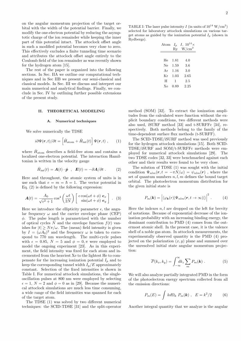
Here we introduce the ellipticity parameter ε, the angu-lar frequency ω and the carrier envelope phase (CEP)φ. The pulse length is parametrized with the numberof optical cycles N and the envelope function f(t) van-ishes for |t| ≥ Nπ/ω. The (mean) field intensity is givenby I = (ωA0)2 and the frequency ω is taken to corre-spond to 770 nm wavelength. The multi-cycle pulseswith ε = 0.85, N = 5 and φ = 0, π were employed tomodel the ongoing experiment [23]. As in this experi-ment, the field intensity was fixed for each atom and in-cremented from the heaviest Xe to the lightest He to com-pensate for the increasing ionization potential Ip and tokeep the corresponding tunnel width Ip/E approximatelyconstant. Selection of the fixed intensities is shown inTable I. For numerical attoclock simulations, the single-oscillation pulses at 800 nm were employed by selectingε = 1, N = 2 and φ = 0 as in [29]. Because the numeri-cal attoclock simulations are much less time consuming,a wide range of the field intensities was spanned for eachof the target atom.

The TDSE (1) was solved by two different numericaltechniques: the SCID-TDSE [31] and the split-operator

TABLE I: The laser pulse intensity I (in units of 1014 W/cm2)selected for laboratory attoclock simulations on various tar-get atoms as guided by the ionization potential Ip (shown inRydbergs).

Atom Ip I, 1014×Ry W/cm2

He 1.81 4.0

Ne 1.59 3.6

Ar 1.16 3.0

Kr 1.03 2.65

H 1 2.5

Xe 0.89 2.25

method (SOM) [32]. To extract the ionization ampli-tudes from the calculated wave function without the ex-plicit boundary conditions, two different methods werealso used, iSURF method [33] and t-SURFFc [34], re-spectively. Both methods belong to the family of thetime-dependent surface flux methods (t-SURFF).

The SCID-TDSE/iSURF method was used previouslyfor the hydrogen attoclock simulations [15]. Both SCID-TDSE/iSURF and SOM/t-SURFFc methods were em-ployed for numerical attoclock simulations [29]. Thetwo TDSE codes [32, 33] were benchmarked against eachother and their results were found to be very close.

The solution of TDSE (1) was sought with the initialcondition Ψnlm(r, t = −πN/ω) = ψnlm(r) , where theset of quantum numbers n, l,m defines the bound targetorbital. The photoelectron momentum distribution forthe given initial state is

Pm(k) =∣∣∣〈ϕk(r)|Ψnlm(r, t→∞)|〉

∣∣∣2 . (4)

Here the indexes n, l are dropped on the left for brevityof notations. Because of exponential decrease of the ion-ization probability with an increasing binding energy, thedominant contribution to PMD (4) comes from the out-ermost atomic shell. In the present case, it is the valenceshell of a noble gas atom. In attoclock measurements, theexperimentally observed quantity is the PMD (4) pro-jected on the polarization (x, y) plane and summed overthe unresolved initial state angular momentum projec-tion:

P (kx, ky) =

∫ ∞−∞dkz

∑m

Pm(k) . (5)

We will also analyze partially integrated PMD in the formof the photoelectron energy spectrum collected from allthe emission directions:

Pm(E) =

∫kdΩk Pm(k) , E = k2/2 (6)

Another integral quantity that we analyze is the angular

3

profile

Pm(θ) =

∫k dk Pm(kx, ky) (7)

k = (k2x + k2y)1/2 , θ = tan−1(ky/kx)

The angular maxima of Pm(θ) serve to determine the at-toclock offset angle θA relative to the minor polarizationaxis of the laser pulse (the axis x in our coordinate frame,see Fig. 1 for illustration).

B. Analytical models

1. Semi-classical approach

We adopt the saddle point method (SPM) [35] whichrelates the photoelectron momentum at the detector k ≡kt→∞ with a specific instant of tunneling ti such that thesemi-classical action along the photoelectron trajectorystarting from this instant

Sk(t) =

∫ t

ti

dt′[k +A(t′)]2/2 + Ip (8)

is stationary:

∂Sk(ti)/∂t = [k + A(ti)]2/2 + Ip = 0 . (9)

In a general case, several solutions of Eq. (9) lead to thefinal photoelectron momentum k and the PMD is givenby the sum over the corresponding tunneling ionizationtimes [16]

Pm(k) ∝NSP∑i=1

∣∣∣∣φnlm(vi)[S′′k(ti)

]−1exp[iSk(ti)]

∣∣∣∣2 . (10)

Here the target orbital in the momentum space φnlm(vi)depends on the initial velocity at the instant of tunnelingvi = k + A(ti) . We note that for very intense fields Ipcan be neglected in Eq. (9) and vi = 0.

For few-cycle circularly or elliptically polarized laserpulses, the number of the saddle points for a given mo-mentum NSP = N + 1 [36]. For a continuous wave whenN → ∞, the solution of (9) can be found analytically[16, 30, 37]. In this case the initial velocity

vi = k0 +A0

[cosh(ωτ0) ex + i sinh(ωτ0) ey

](11)

In the tunneling ionization regime, the Keldysh parame-ter γ = ωτ0 . 1 and Eq. (11) can be reduced to

vxi ' A0γ2/3 , vyi ' iA0γ = iκ . (12)

The purely imaginary intial velocity vxi is related to thelinear momentum of the bound electron κ =

√2Ip.

The target orbital factor in Eq. (10) brings in the an-gular momentum projection dependence

Pm(k) ∝ | exp(imφv)|2 , tanφv = vyi/vxi (13)

In the case of an np target orbitals, Eq. (11) leads to

Pnp−1(k0)

Pnp+1(k0)=|3 + γ|2

|3− γ|2' 1 +

4γ

3as γ → 0 (14)

Here k0 = A0 sinh(ωτ0)/(ωτ0) defines the peak positionof the PMD in the semi-classical model.

FIG. 1: Polarization ellipse of the laser field. The electricfield E(t0) along y defines the direction of tunneling and thetunneling width y0. The initial velocity in this direction vyiin (12) is purely imaginary. The vector potential A(t0) alongx defines the photoelectron momentum at the detector kt→∞and the attoclock offset angle θA. The initial velocity alongthis direction vxi in (12) is real. The classical velocity of theorbital motion vm=±1 adds up to the real velocity vxi at theexit from the tunnel.

2. Classical considerations

The semi-classical action (8) and the SPM equation (9)do not differentiate the photoelectron trajectories withrespect to them projection. It is only the pre-exponentialmagnitude factor in Eq. (10) that makes the m = ±1 ion-ization probabilities differ. Identical trajectories wouldmean the same angular profiles and the attoclock offsetangles. However, various numerical simulations do notsupport this scenario. As was shown earlier [20, 22] andwill be demonstrated in the following, the offset anglesin noble gas atoms differ substantially and systematicallyfor m = ±1. In previous works [20, 22], this differencewas attributed to variation of the tunnel width and astronger effect of the Coulomb field of the ion remain-der when the photoelectron leaves the atom closer to theionic core. To investigate this effect further, we employhere the following classical models.

a. Neglect of the Coulomb field This model is ex-pected to work in strong laser fields where the Coulombfiled of the ion remainder can be neglected. We define thephotoelectron trajectory in the laser field by the classicalequations of motion

r(t) =

∫ t

t0

A(τ)dτ + vf (t− t0) + r0 . (15)

Here vf = v0 −A(t0) is the final velocity after the pulseend and v0 = v(t0) is the initial velocity. The vectorpotential (3) is rewritten here as

Ax(t) = −Ax0f(t) cosω(t− t0) (16)

Ay(t) = Ay0f(t) sinω(t− t0) ,

where the envelope f(t0) = 1, f(t → ∞) = 0 and the

magnitudes Ax0 = εA0/√

1 + ε2 < Ay0 = A0/√

1 + ε2.The peak electric field at t0 is directed along y and thephotoelectron exit point r0 = (0, y0). We assume thatf(t) varies slowly. Under this assumption, the photoelec-

4

tron trajectory (15) can be expressed as

x(t) = −bf(t) sinω(t− t0) + vf (t− t0) (17)

y(t) = −a[f(t) cosω(t− t0)− 1] + y0 ,

where a = Ay0/ω and b = Ax0/ω, vf = v0 + Ax0. Afterthe pulse end, the trajectory becomes a straight line

x(t→∞) = vf (t− t0) (18)

y(t→∞) = ξa+ y0 .

Here we introduce a parameter ξ to account for a finitepulse duration. With an accuracy to 1/N4,

ξ = 1 + 1/N2 . (19)

We relate the angular momentum projection of thebound electron m with its orbital velocity at the exitfrom the tunnel as shown schematically in Fig. 1. Thuswe augment the initial velocity after the tunneling vxigiven by Eq. (12) in the strong field limit with this clas-sical velocity:

v0 = vxi +m/y0 , (20)

where the tunnel width

y0 ' Ip/(ωAy0). (21)

The initial momentum projection of the photoelectron atthe exit from the tunnel

m0 = v0y0 = m+ vxiy0 = m+M0γ2/3 , (22)

where M0 = Ax0y0 ' εIp/ω is the parameter sensitive toy0. In the case when y0 satisfies Eq. (21), M0 is propor-tional to the minimum number of the absorbed photonsneeded to bridge the ionization potential gap N0 = Ip/ω.The final photoelectron angular momentum projection atthe detector

M = vf (ξa+ y0) (23)

= m+ (1 + ξ/3)M0 +

(1 +

m

M0

)2ξE0εω

.

Here

E0 =A2x0

2=

2ε2

1 + ε2Up (24)

and the ponderomotive energy

Up = A20/4 (25)

Similarly, the final photoelectron energy is

E =(Ax0 + v0)2

2' ε2Ip

3+

(1 +

2m

M0

)E0 (26)

At large field intensities, deep in the tunneling regime,M0 m0. For long laser pulses N 1 leads to ξ =1. In this case, the photoelectron momentum projectiongain can be expressed via the photoelectron energy at thedetector:

∆M = M −m ' 2ε

1 + ε2Ip + Up + E

ω. (27)

This expression relates the angular momentum projec-tion gain of the photoelectron with the number of ab-sorbed photons via the law of energy conservation.

b. Neglect of the laser field For low laser field inten-sity and short pulse duration, the photoelectron trajec-tory is determined largely by the Coulomb field of theion remainder. To determine such a trajectory, the clas-sical Rutherford scattering model can be applied [28]. Inthis model, the distance of the closest approach in theRutherford formula is equated with the tunnel width y0whereas the asymptotic electron velocity at the infinitycorresponds to the peak vector potential A0. The result-ing attoclock offset angle is expressed as

tan θA =ω2

E20

Z∗

y0=

1

k20

Z∗

y0. (28)

For neutral atomic targets, the asymptotic charge of theion remainder Z∗ = 1. When this charge is fully screenedlike in negative ions [38] or in the Yukawa potential [15],Z∗ = 0 and θA → 0. We will use this property in ourfurther TDSE simulations in Sec. III D when we reducethe asymptotic charge of the ion remainder to observethe vanishing angular offset.

Expression (28) was tested against numerical atto-clock TDSE calculations for atomic hydrogen and demon-strated its validity for very weak field. It is not expectedto be rigorously valid in the field range considered here.Nevertheless, we use it to estimate a characteristic dis-tance where the Coulomb field makes its strongest effecton the photoelectron motion. We invert Eq. (28) andexpress the distance of the closest approach of the pho-toelectron to the ionic core via the attoclock offset angleand the peak photoelectron momentum, both quantitiesknown from our TDSE calculations:

ym0 =C

tan θA

1

k2m0

(29)

The numerical constant C is chosen to scale the attoclockoffset angle θA(m = 0) with the tunnel width y0.

III. RESULTS AND DISCUSSION

A. Numerical vs laboratory attoclock

The difference between the laboratory and numericalattoclocks with long and short pulses, respectively, is il-lustrated in Fig. 2. Here the numerical attoclock resultsare exhibited in the top row of panels while analogousresults for the laboratory attoclock are displayed in thebottom row. For illustrative purposes, we consider theAr 3p photoionization by a single-cycle 2.9 fs pulse at0.86 × 1014 W/cm2 (top) and a multi-cycle 6.8 fs pulseat 3× 1014 W/cm2 (bottom).

5

Vector potential A(t) Saddle point simulation TDSE simulation

-0.6

-0.4

-0.2

0

0.2

0.4

0.6

-0.8 -0.6 -0.4 -0.2 0 0.2 0.4

Ay(t

) (a

.u.)

Ax(t) (a.u.)

N=2

-1

-0.5

0

0.5

1

-1 -0.5 0 0.5 1

Ay(t

) (a

.u.)

Ax(t) (a.u.)

N=7

-1.5 -1.0 -0.5 0.0 0.5 1.0 1.5

kx (a.u.)

-1.5

-1.0

-0.5

0.0

0.5

1.0

1.5 k

y (

a.u

.)

0.0000

0.0005

0.0010

0.0015

0.0020

0.0025

-1.5 -1.0 -0.5 0.0 0.5 1.0 1.50.0

kx (a.u.)

-1.5

-1.0

-0.5

0.0

0.5

1.0

1.5

0.0

ky (

a.u

.)

0.000

0.005

0.010

0.015

0.020

0.025

0.030

FIG. 2: From left to right: the parameteric plots of the vector potential A(t), the PMD (4) from the SPM simulations andthat of the TDSE simulations. The top row of panels corresponds to the argon atom ionized with a nearly single-cycle 2.9 fspulse at 0.86 × 1014 W/cm2. The bottom row of panels visualizes the same ionization process driven by a multi-cycle 6.8 fspulse at 3 × 1014 W/cm2

The parametric plots in the left column represent thevector potential A(t) (3) with N = 2 (top) and N = 7(bottom). Solutions of the SPM equation (9) correspond-ing to a given photoelectron momentum k can be visual-ized graphically by the intersects of A(t) with the straight

line pointing into the k direction. Indeed, if Ip can beneglected in (9), then simply k = −A(ti). In a generalcase, three solutions can be identified for a short pulsewith N = 2 of which two correspond to small values of|A(ti)| and do not contribute significantly to PMD. Theremaining “dominant” solution produces a well formedlobe of intensity in the PMD graph shown in the topcentral panel. This image is obtained with an exponen-tial accuracy visualizing the kinematic factor

NSP∑i

[S′′k(ti)

]−1exp[iSk(ti)] ,

while neglecting the squared momentum space orbital inthe pre-exponential term. In the top right panel, we dis-play a very similar PMD image returned by the TDSEcalculation. The only visible difference between the topcentral and right panels is a rotation of the whole PMDby an attoclock offset angle θA. This rotation is entirelydue to the Coulomb field which is neglected in the SPM.

The number of solutions in the case of a multi-cyclepulse is significantly greater. The 8 solutions can beidentified graphically in each of the positive and negativemomentum directions. Accordingly, the PMD is sym-

metric in the ±kx direction as is shown in the bottomcentral panel of Fig. 2. The ATI rings coming from themanifold of the SPM solutions are clearly visible in thispanel. Again, as in the case of a short pulse visualizedin the top row, the TDSE solution returns a very similarPMD image except for the angular rotation. Because ofa number of ATI rings tilted differently, there is no singleattoclock offset angle θA that can be easily identified tocharacterize the Coulomb field effect.

Further distinction between the numerical and labora-tory attoclock is illustrated in Figs. 3 and 4 where we plotthe corresponding photoelectron spectra (6) and their an-gular profiles (7), respectively. The energy spectra of thenumerical and laboratory attoclock are shown in the topand bottom panels of Fig. 3, respectively. These spec-tra differ by the profound ATI structure on the formerand its absence on the latter. Intensity varies dramati-cally between the magnetic projections with m = 0 beingstrongly suppressed by the angular node of the target 3porbital in the polarization plane. As to the other twoprojections, the ratio Pm=−1/Pm=1 1 in line withEq. (14). More detailed analysis of this ratio will beconducted in Section III B.

Eq. (27) allows to relate the photoelectron spectrumPm(E) with the angular momentum projection profilewith the angular momentum projection profile calculatedas Pm(M) ' ωPm(E). Except for very low photoelectronenergy, the Pm(E) and Pm(M) profiles match each otherrather well, both for the numeric (Fig. 3 top) and labo-

6

0

0.05

0.1

0.15

0.2

0 0.2 0.4 0.6 0.8 1

0.2 0.6 0.7 1.2

Sp

ectr

um

Pm

(E)

(10

-4 a

u)

Energy E (au)

Momentum (au)

Ar 3p 0.86×1014

W/cm2

10× m= 0 m= 1

0.1× m=-1Pm(M) m=-1

m= 0

0

0.5

1

0 0.5 1 1.5

0.2 0.6 0.7 1.2 1.5

Sp

ectr

um

Pm

(E)

(10

-2 a

u)

Energy E (au)

Momentum (au)

Ar 3p 3×1014

W/cm2

10×m=0m=1

0.5×m=-1Pm(M) m=-1

FIG. 3: Photoelectron spectrum (6) of Ar 3p ionized with asingle-cycle pulse at 0.86 × 1014 W/cm2 (top) and a multi-cycle pulse at 3 × 1014 W/cm2 (bottom). Various m spectraare scaled up and down for to fit the figure. The correspondingorbital momentum projection profiles Pm(M) are convertedto the photoelectron energy scale by Eq. (27) and overplotted.

ratory (Fig. 3 bottom) attoclocks.The angular profiles of the numerical and laboratory

attoclocks are displayed in the top and bottom panels ofFig. 4, respectively. While there is a single maximumin the angular profile of the numerical attoclock, thereare two symmetric maxima in the case of the laboratoryattoclock. Positions of the respected maxima are locatedby the Gaussian fitting illustrated in Fig. 4 for m = −1profiles. Similar to the energy spectra, the angular pro-files differ strongly in magnitude. The angular maximapositions are also displaced between various m projec-tions.

B. Target orbital structure effect

In this section, we examine the target orbital struc-ture effect on various observables returned by the TDSEcalculations. As a case study, we consider the numericalattoclock on Ar 3pm driven at λ = 800 nm by a circu-larly polarized single-oscillation pulse. The field inten-sity range starts from modestly non-adiabatic tunnelingregime at γ ' 2 and ends below the onset of the over-the-barrier ionization regime at IOBI ' 1015 W/cm2 [39].

In the top panel of Fig. 5 we plot the peak values of the

0

0.2

0.4

0.6

-180 -120 -60 0 60 120 180

Pm

(θ)

(1

0-4

au

)

Polar angle θ (deg)

θA

Ar 3p 0.86×1014

W/cm2

103× m= 0

7× m= 1m=-1

Gaussian

0.2

0.4

0.6

0.8

1

-180 -90 0 90 180

Pm

(θ)

(1

0-2

au

)

Polar angle θ (deg)

θA

Ar 3p 3×1014

W/cm2

20× m= 02× m= 1

m=-1Σm

Gauss

FIG. 4: Angular profiles (7) of the Ar 3p ionized with a single-cycle pulse at 0.86×1014 W/cm2 (top) and a multi-cycle pulseat 3 × 1014 W/cm2 (bottom). Various m profiles are scaledfor better clarity. A Gaussian fit is used to locate positionsof the corresponding angular maxima. The angular maximaof the m = −1 profiles are marked with the vertical dottedlines which define the corresponding attoclock offset anglesθA. The bottom panel show the PMD (4) integrated radiallyand marked as Σm.

photoelectron momentum projection gain ∆M = M −mas obtained from the TDSE solution and as prescribed byEq. (23). The latter equation predicts the linear increaseof ∆M with the field intensity which is indeed the case.In the weak field regime, Eq. (23) is no longer valid andthe numerical results deviate from the predicted asymp-totic limit ∆M = N0(1 + ξ/3). Both the numerical andanalytical results for various m converge for low fieldsbut deviate noticeably as the laser field grows. The ∆Mgain is strongest for m = 1 and the weakest for m = −1.This can be understood from the m-dependent term inEq. (23) which appears due to the orbital velocity termm/y0 in Eq. (20) under assumption of the tunnel widthy0 independent of m. Because the analytical predictionsof Eq. (23) agree well with the numerical TDSE resultsfor all m, it can suggest that the actual tunnel widthis indeed independent of m, at least in the strong fieldregime.

In the second top panel of Fig. 5 we plot the peakphotoelectron momentum corresponding to maxPm(E).While the peak momentum values are rather close form = 0 and m = 1, they are noticeably smaller form = −1. In the same graph, we plot the peak vectorpotential A0 which adds up with the initial velocity ofthe photoelectron v0x > 0 at the instant of tunneling.Accordingly, the peak photoelectron momentum at thedetector exceeds A0 for m = 0, 1. This is not so for

7

10

20

30

40

50

60

0 1 2 3 4 5

2 1 0.8 0.7 0.6 0.5

Mom

entu

m p

roje

ction g

ain

M-m

Keldysh parameter γ

Ar 3p λ=800nm

N0(1+ξ/3)

TDSE m= 0 m=+1

m=–1Eq. (23) m= 0

m=+1m=–1

0.6

0.8

1

1.2

1.4

0 1 2 3 4 5

Peak m

om

entu

m k

m0 (

au)

Ar 3p λ=800nm

TDSE m= 0

m=+1m=–1

A0

5

10

15

20

0 1 2 3 4 5

Attoclo

ck o

ffset angle

θA (

deg)

Ar 3p λ=800nm TDSE m= 0m=+1m=–1

KR m= 0 m=+1 m=–1

5

10

15

20

25

0 1 2 3 4 5

Clo

se

st

ap

pro

ach

ym

0 (

au

)

Field intensity (1014

W/cm2)

Ar 3p λ=800nmTDSE m= 0

m=+1m=–1

Tunnel width Ip/E0

FIG. 5: Various observables returned by TDSE calculationson Ar 3pm driven by a short pulse at 800 nm. Top: the gain ofthe photoelectron momentum projection ∆M Eq. (27). Thelow field limit ∆M = N0(1+ξ/3) of Eq. (23) is shown with thedotted line. Second top: peak photoelectron momentum km0

is compared with the vector potential A0. Second bottom:the attoclock offset angle θA. Bottom: the distance of theclosest approach ym0 (29). The tunnel width y0 = Ip/E0 isalso visualized.

m = −1. In this case, the initial velocity changes its signcontrary to semi-classical expression (11) which is alwayspositive. Eq. (20) augments v0x with the classical orbitalvelocity m/y0 which is negative for m = −1 and growsas the field intensity increases and the tunnel width y0decreases. This explains the observed effect visible in thefigure.

0

5

10

15

20

0 2 4 6 8 10

2 1 0.8 0.6 0.5 0.4

Pm

=-1

(k0)/

Pm

=1(k

0)

Field intensity, 1014

W/cm2

Keldysh parameter γ

Ar 3p λ=800nmTDSE

SPM

|3+γ|2/|3-γ|

2

FIG. 6: Ratio of the peak momentum profile values for Ar3pm=±1 compared with semi-classical prediction Eq. (14).

In the second bottom panel, we display the attoclockoffset angles θA. Again, as in the case of the peak momen-tum values, the m = −1 projection is noticeably differentfrom the two other m. When comparison is made withthe KR formula (28), the coefficient C = 2 is deducedfor m = 0. The TDSE results for m = 1 agree well withthe KR in the low field regime but start to deviate whenthe field intensity grows. The TDSE results for m = −1significantly overshoot the KR formula prediction thusinvalidating the assumption of the constant y0 indepen-dent of m.

Indeed, when the KR formula is inverted to the dis-tance of the closest approach by Eq. (29), this is trans-lated to the photoelectron approaching the ionic coremuch closer in the m = −1 case as indicated in the bot-tom panel of Fig. 5. For all the m values, the closestapproach distance shown in the bottom panel of Fig. 7displays a 1/

√I scaling with the field intensity which is

characteristic for the tunnel width y0 = Ip/E0.

Eq. (14) predicts the m = ±1 ratio of the peak valuesof the momentum profiles as determined by the semi-classical SPM expression (10) for a continuous oscillationwave. In Fig. 9 we compare Eq. (14) for Ar 3p withthe TDSE and SPM results for a short pulse at λ =800 nm. Both results agree with the SPM predictioneven for not so small Keldysh parameters γ ' 1 in amildly non-adiabatic tunneling regime. At larger fieldintensities, the TDSE result approaches the γ → 0 limitfaster than the SPM result.

C. Comparison between various atoms

To make a comparison of the attoclock offset anglesbetween various members of the noble gas family, we takethe experimentally measurable PMD (4) and subject itto a radial integration

∫kdk. In doing so we discard

the m dependence which is not resolved experimentally.Such an angular profile is displayed in the bottom panelof Fig. 4 and marked as Σm along with the m-resolvedangular profiles. Not surprisingly, the m-summed profile

8

2

5

10

20

0.5 1 2 5

Attoclo

ck o

ffset angle

θA (

deg)

Intensity (1014

W/cm2)

Atoms H KrArNeHe

FIG. 7: Attoclock offset angles of various atoms versus drivingpulse intensity. The numerical attoclock results with a shortpulse are marked with dotted lines. The laboratory attoclockvalues with a multi-cycle driving pulse at selected field inten-sities and m = −1 are shown with error bars of the matchingplotting style.

is very close to the dominant in magnitude m = −1 one.Thus obtained angular profiles are fitted with a Gaussianansatz and the positions of the respected angular maximaare obtained. The offset of these maxima relative to theminor polarization x axis gives the attoclock offset anglesθA which are displayed in Fig. 7. The error bars shown inthe figure result from a deviation of the angular profilesfrom a Gaussian shape noticeable in the bottom panelof Fig. 4. In the same Fig. 7 we display the offsetangles for the numerical attoclock across a range of fieldintensities. To make a comparison with the laboratoryattoclock, we select the dominant m = −1 projection.The angular profiles of the numerical attoclock have aperfect Gaussian shape, so the error bars are negligiblehere.

The numerical attoclock offset angles become smalleras the ionization potential of the atom grows. This de-crease of θA is in line with the prediction of the KRformula (28) and can be explained by the larger tunnelwidth y0 = Ip/E0. The hydrogen atom deviates some-what from this tendency. This may be a subtle effect ofits electronic structure which is different from the noblegas atoms. A sharp decrease of θA for hydrogen towardsthe higher end of the field intensities reflects the onset ofthe over-the-barrier regime at IOBI ' 0.5× 1014 W/cm2

[39].

The laboratory attoclock offset angles are generally inline with their numerical counterparts. Because the fixedfield intensities in the laboratory attoclock simulationsshown in Table I are selected to maintain approximatelythe same nominal tunnel width y0 = Ip/E0, it is instruc-tive to apply Eq. (29) and to compare the distance of theclosest approach across the various target atoms. Thiscomparison is made in Fig. 8. It is the m = −1 pro-jection that makes the strongest contribution to the m-average offset angles. For this projection, the attoclock

5

10

15

20

25

0 1 2 3 4 5

Clo

se

st

ap

pro

ach

ym

0 (

au

)

Field intensity (1014

W/cm2)

Ar 3p λ=800nmTDSE m= 0

m=+1m=–1

Tunnel width Ip/E0

FIG. 8: The distance of the closest approach obtained withEq. (29) for various atoms is compared with the correspondingtunnel width 0.5Ip/E0.

offset angle is the largest and the distance of the closestapproach is the smallest which is demonstrated for Arin bottom panel of Fig. 5. The same is true for all theatoms displayed in Fig. 8 where the distance of the clos-est approach is about half of the nominal tunnel widthy0/2 = 0.5Ip/E0.

D. Coulomb field effect

The KR expression (28) for the attoclock offset anglecontains the asymptotic charge Z∗ of the ion remainder.In this section, we treat this charge as an adjustable pa-rameter. To do so, we modify the one-electron potentialV (r) entering the atomic Hamiltonian Hatom and reduceZ∗ gradually to zero. In this way we aim to eliminate theCoulomb field effect on the attoclock offset angle. Theeffective charge can be expressed via the one-electron po-tential as Z(r) = −rV (r) and the asyimptotic value en-tering Eq. (28) is Z∗ = Z(r →∞) .

In Fig. 6 we plot Z(r) for various one-electron poten-tials used in our calculations for Ar. These are an empir-ical Tong [05] potential [40] and a localized Hartree-Fock(LHF) potential [41]. The latter potential has a simpleanalytical form

ZHF(r) = (Z0 − Z∗)e−r/λ + Z∗ ,

where Z0 is the bare nucleus charge and λ is a screeninglength. In our simulations, we gradually decrease Z∗ inseveral steps as shown in Fig. 6. At the same time we ad-just λ to maintain the binding energy of the 3p electronin Ar. The resulting PMD projected on the polariza-tion plane (4) are exhibited in Fig. 10. The top panelshould be compared with the top right panel of Fig. 2where the empirical potential from [40] was used. As Z∗

is gradually diminished, so is the offset angle which isreduced virtually to zero when Z∗ = 0.25. Interestingly,the ionization probability is falling sharply when the Z∗

is decreasing. This is because the photoelectron becomesasymptotically free and cannot any longer absorb pho-tons.

9

0.1

1

10

0.1 1 10

0.25

0.5

Z*=1

Eff

ective

ch

arg

e Z

(r)=

rV(r

)

Radius (au)

ArgonTong [05]

LHF Z=1.00.5

0.25

FIG. 9: Effective charge in Ar expressed via various one-electron potentials. The asymptotic values Z∗ for vari-ous modifications of the localized Hartree-Fock potential aremarked on the left vertical scale.

IV. CONCLUSIONS AND FURTHERDIRECTIONS

We have studied systematically tunneling ionization ofnoble gas atoms with close to circularly polarized laserpulses in the attoclock field configuration. We simulatedboth the numerical and laboratory attoclocks driven byshort, nearly single-cycle pulses and much longer multi-cycle pulses, respectively. Our numerical attoclock sim-ulations covered a range of field intensities from a mildlynon-adiabatic tunneling regime to the onset of over-the-barrier ionization. The laboratory attoclocks were simu-lated at selected energies while maintaining an approxi-mately constant tunnel width.

We analyzed various observables generated from solu-tions of the time-dependent Scrodinger equation in thesingle active electron approximation. We also employedthe semi-classical strong field ionization theory based onthe saddle-point approximation, both in the analyticalform for continuous waves and implemented numericallyfor short pulses.

We examined the peak values of the photoelectron lin-ear momentum and the angular momentum projectionsas well as the attoclock offset angle. From these quanti-ties we were able to derive the characteristic distance ofthe photoelectron approach to the Coulomb center of theionic core. This distance was compared with the nominaltunnel width in the semi-classical theory of strong fieldionization. All these parameters demonstrate a strongdependence on the m-projection of the initial boundstate. While the m = 0 and m = 1 values were foundcomparable, the m = −1 projection produced a notice-able deviation. This deviation was particularly strong forthe attoclock offset angles. In our field configuration, them = −1 projection corresponds to the circularly polar-ized field counter-rotating with the electron cloud in theinitially bound state. Electrons with this m-projectionare much more easily ionized and escape the potentialbarrier much closer to the ionic core. It is for this reasonthat their Coulomb deflection is stronger. The latter ef-fect was effectively turned off by reducing the asymptoticcharge of the ionic core.

LHF Z=1

-1.5 -1.0 -0.5 0.0 0.5 1.0 1.5

kx (a.u.)

-1.5

-1.0

-0.5

0.0

0.5

1.0

1.5

ky (

a.u

.)

0

2×10-5

4×10-5

6×10-5

8×10-5

LHF Z=0.5

-1.5 -1.0 -0.5 0.0 0.5 1.0 1.5

kx (a.u.)

-1.5

-1.0

-0.5

0.0

0.5

1.0

1.5

ky (

a.u

.)

0

1×10-6

2×10-6

3×10-6

LHF Z=0.25

-1.5 -1.0 -0.5 0.0 0.5 1.0 1.5 kx (a.u.)

-1.5

-1.0

-0.5

0.0

0.5

1.0

1.5

ky (

a.u

.)

0

1×10-7

2×10-7

3×10-7

4×10-7

5×10-7

FIG. 10: The PMD (4) of Ar 3p driven by a single-cycle pulseat 0.86 × 1014 W/cm2. The asymptotic charge of the ionremainder is reduced in the LHF potential from Z∗ = 1 (top)to 0.5 (middle) and 0.25 (bottom).

We hope that our numerical results and their theo-retical interpretation will guide the next generation oflaboratory attoclock studies on noble gas atoms. Theseexperiments are currently underway. [23].Acknowledgment We gratefully acknowledge Igor

Litvinyuk, Robert Sang and Satya Sainadh for manystimulating discussions. We thank Serguei Patchkovskiifor placing his iSURF TDSE code at our disposal. AlexBray let us use his Mathematica script for SPM com-putations. Resources of National Computational Infras-tructure facility (NCI Australia) have been employed.

10

[1] C. P. J. Martiny, M. Abu-samha, and L. B. Madsen, Ion-ization of oriented targets by intense circularly polarizedlaser pulses: Imprints of orbital angular nodes in the two-dimensional momentum distribution, Phys. Rev. A 81,063418 (2010).

[2] M. Abu-samha and L. B. Madsen, Alignment dependenceof photoelectron momentum distributions of atomic andmolecular targets probed by few-cycle circularly polarizedlaser pulses, Phys. Rev. A 94, 023414 (2016).

[3] L. Arissian, C. Smeenk, F. Turner, C. Trallero, A. V.Sokolov, D. M. Villeneuve, A. Staudte, and P. B.Corkum, Direct test of laser tunneling with electron mo-mentum imaging, Phys. Rev. Lett. 105, 133002 (2010).

[4] I. A. Ivanov, A. S. Kheifets, J. E. Calvert, S. Goodall,X. Wang, H. Xu, A. J. Palmer, D. Kielpinski, I. V.Litvinyuk, and R. T. Sang, Transverse electron momen-tum distribution in tunneling and over the barrier ioniza-tion by laser pulses with varying ellipticity, Sci. Rep. 6,19002 (2016).

[5] P. Eckle et al, Attosecond angular streaking, Nat. Phys.4, 565 (2008).

[6] P. Eckle, M. Smolarski, P. Schlup, J. Biegert, A. Staudte,M. Schoffler, H. G. Muller, R. Dorner, and U. Keller,Attosecond angular streaking, Nat Phys 4, 565 (2008).

[7] A. N. Pfeiffer, C. Cirelli, M. Smolarski, D. Dimitrovski,M. Abu-samha, L. B. Madsen, and U. Keller, Attoclockreveals natural coordinates of the laser-induced tunnellingcurrent flow in atoms, Nat Phys 8, 76 (2012).

[8] M. Han, P. Ge, Y. Shao, Q. Gong, and Y. Liu, Atto-clock photoelectron interferometry with two-color corotat-ing circular fields to probe the phase and the amplitudeof emitting wave packets, Phys. Rev. Lett. 120, 073202(2018).

[9] M. Han, P. Ge, Y. Fang, X. Yu, Z. Guo, X. Ma, Y. Deng,Q. Gong, and Y. Liu, Unifying tunneling pictures ofstrong-field ionization with an improved attoclock, Phys.Rev. Lett. 123, 073201 (2019).

[10] R. Boge, C. Cirelli, A. S. Landsman, S. Heuser, A. Lud-wig, J. Maurer, M. Weger, L. Gallmann, and U. Keller,Probing nonadiabatic effects in strong-field tunnel ioniza-tion, Phys. Rev. Lett. 111, 103003 (2013).

[11] A. S. Landsman, M. Weger, J. Maurer, R. Boge, A. Lud-wig, S. Heuser, C. Cirelli, L. Gallmann, and U. Keller,Ultrafast resolution of tunneling delay time, Optica 1(5),343 (2014).

[12] N. Camus, E. Yakaboylu, L. Fechner, M. Klaiber,M. Laux, Y. Mi, K. Z. Hatsagortsyan, T. Pfeifer, C. H.Keitel, and R. Moshammer, Experimental evidence forquantum tunneling time, Phys. Rev. Lett. 119(2), 023201(2017).

[13] C. Hofmann, A. S. Landsman, and U. Keller, Attoclockrevisited on electron tunnelling time, J. of Modern Optics66(10), 1052 (2019).

[14] A. S. Kheifets, The attoclock and the tunneling time de-bate, J. Phys. B 53(7), 072001 (2020).

[15] U. S. Sainadh, H. Xu, X. Wang, A. Atia-Tul-Noor, W. C.Wallace, N. Douguet, A. Bray, I. Ivanov, K. Bartschat,A. Kheifets, et al., Attosecond angular streaking and tun-nelling time in atomic hydrogen, Nature 568, 75 (2019).

[16] I. Barth and O. Smirnova, Nonadiabatic tunneling in cir-cularly polarized laser fields: Physical picture and calcu-lations, Phys. Rev. A 84, 063415 (2011).

[17] I. Barth and O. Smirnova, Spin-polarized electrons pro-duced by strong-field ionization, Phys. Rev. A 88, 013401(2013).

[18] D. Trabert, A. Hartung, S. Eckart, F. Trinter, A. Kalinin,M. Schoffler, L. P. H. Schmidt, T. Jahnke, M. Kunitski,and R. Dorner, Spin and angular momentum in strong-field ionization, Phys. Rev. Lett. 120, 043202 (2018).

[19] I. A. Ivanov and A. S. Kheifets, Time delay in atomicphotoionization with circularly polarized light, Phys. Rev.A 87, 033407 (2013).

[20] Y. Li, P. Lan, H. Xie, M. He, X. Zhu, Q. Zhang, andP. Lu, Nonadiabatic tunnel ionization in strong circularlypolarized laser fields: counterintuitive angular shifts inthe photoelectron momentum distribution, Opt. Express23(22), 28801 (2015).

[21] J.-P. Wang and F. He, Tunneling ionization of neonatoms carrying different orbital angular momenta instrong laser fields, Phys. Rev. A 95, 043420 (2017).

[22] Q. Zhang, G. Basnayake, A. Winney, Y. F. Lin, D. De-brah, S. K. Lee, and W. Li, Orbital-resolved nonadiabatictunneling ionization, Phys. Rev. A 96, 023422 (2017).

[23] Satya Sainadh Undurti, Robert Sang and Igor Litvinyuk(2020), private communication.

[24] M.-H. Yuan and X.-B. Bian, Angular distribution ofphotoelectron momentum in above-threshold ionizationby circularly polarized laser pulses, Phys. Rev. A 101,013412 (2020).

[25] L. Torlina, F. Morales, J. Kaushal, I. Ivanov, A. Kheifets,A. Zielinski, A. Scrinzi, H. G. Muller, S. Sukiasyan,M. Ivanov, et al., Interpreting attoclock measurements oftunnelling times, Nature Physics 11(6), 503 (2015).

[26] H. Ni, U. Saalmann, and J.-M. Rost, Tunneling ioniza-tion time resolved by backpropagation, Phys. Rev. Lett.117, 023002 (2016).

[27] J. Liu, Y. Fu, W. Chen, Z. L, J. Zhao, J. Yuan, andZ. Zhao, Offset angles of photocurrents generated in few-cycle circularly polarized laser fields, J. Phys. B 50(5),055602 (2017).

[28] A. W. Bray, S. Eckart, and A. S. Kheifets, Keldysh-Rutherford model for the attoclock, Phys. Rev. Lett.121(12), 123201 (2018).

[29] V. V. Serov, A. W. Bray, and A. S. Kheifets, Numericalattoclock on atomic and molecular hydrogen, Phys. Rev.A 99, 063428 (2019).

[30] A. Perelomov, V. Popov, and M. Terent’ev, Ionizationof atoms in an alternating electric field II, Sov. Phys. –JETP 24(1), 207 (1967).

[31] S. Patchkovskii and H. Muller, Simple, accurate, andefficient implementation of 1-electron atomic time-dependent schrdinger equation in spherical coordinates,Computer Physics Communications 199, 153 (2016).

[32] V. V. Serov, Calculation of intermediate-energy electron-impact ionization of molecular hydrogen and nitrogen us-ing the paraxial approximation, Phys. Rev. A 84, 062701(2011).

[33] F. Morales, T. Bredtmann, and S. Patchkovskii, iSURF:a family of infinite-time surface flux methods, J. Phys. B49(24), 245001 (2016).

[34] V. V. Serov, V. L. Derbov, T. A. Sergeeva, and S. I.Vinitsky, Hybrid surface-flux method for extraction of theionization amplitude from the calculated wave function,Phys. Rev. A 88, 043403 (2013).

11

[35] M. Ivanov, Ionization in Strong Low-Frequency Fields,Attosecond and XUV Spectroscopy: Ultrafast Dynamicsand Spectroscopy (Wiley-VCH, 2014), pp. 179–200, 1sted.

[36] D. B. Milosevic, G. G. Paulus, D. Bauer, and W. Becker,Above-threshold ionization by few-cycle pulses, J. Phys.B 39(14), R203 (2006).

[37] V. D. Mur, S. V. Popruzhenko, and V. S. Popov, En-ergy and momentum spectra of photoelectrons under con-ditions of ionization by strong laser radiation (the case ofelliptic polarization), Sov. Phys. -JETP 92, 777 (2001).

[38] N. Douguet and K. Bartschat, Attoclock setup with nega-tive ions: A possibility for experimental validation, Phys-

ical Review A 99(2), 023417 (2019).[39] Toru Morishita, Keldysh parameter calculator (2020),

online, URL http://power1.pc.uec.ac.jp/~toru/

keldysh/.[40] X. M. Tong and C. D. Lin, Empirical formula for static

field ionization rates of atoms and molecules by lasers inthe barrier-suppression regime, J. Phys. B 38(15), 2593(2005).

[41] A. W. Bray, F. Naseem, and A. S. Kheifets, Simulationof angular-resolved RABBITT measurements in noble-gas atoms, Phys. Rev. A 97, 063404 (2018).