numerical assessment of reverse-flow mufflers using a...

NUMERICAL ASSESSMENT OF REVERSE-FLOW MUFFLERS USING ASIMULATED ANNEALING METHOD

Min-Chie ChiuDepartment of Automatic Control Engineering, Chungchou Institute of Technology, Yuanlin, Changhua 51003, R.O.C.

E-mail: [email protected]

Received December 2008, Accepted March 2010

No. 08-CSME-45, E.I.C. Accession 3117

ABSTRACT

Because of the necessity of maintenance and operation in industries in which the equipment layoutis occasionally tight, the space for a muffler is constrained. An interest in maximizing the acousticalperformance of mufflers within a limited space is of paramount importance. As mufflers hybridizedwith reverse-flow ducts may visibly increase acoustical performance, the main purpose of this paperis to numerically analyze and maximize their acoustical performance within a limited space. In thispaper, a four-pole system matrix for evaluating the acoustic performance —sound transmission loss(STL)— is derived by using a decoupled numerical method. Moreover, simulated annealing (SA), arobust scheme used to search for the global optimum by imitating the metal annealing process, hasbeen used during the optimization process. Before dealing with a broadband noise, the STL’smaximization with respect to a one-tone noise (300 Hz) is introduced for a reliability check on the SAmethod. Moreover, an accuracy check of the mathematical model is performed. Results reveal thatthe STL of a muffler with reverse-flow perforated ducts can be maximized at the desired frequencyfor pure tone elimination; moreover, the noise reduction for a broadband noise can reach 97.5 dB.Consequently, the approach used for the optimal design of the mufflers is simple and effective.

METHODE DU RECUIT SIMULE POUR L’EVALUATION NUMERIQUE DEL’ECOULEMENT INVERSE D’UN SILENCIEUX

RESUME

Dans l’industrie ou la configuration de l’espace pour l’appareillage est parfois limitee, et a causede la necessite de faire de la maintenance, ainsi que pour l’operation de l’appareillage, l’espace pourun silencieux est restreint. L’interet de maximiser la performance acoustique des silencieux al’interieur d’un espace limite est d’une importance capitale. Etant donne que des silencieux hybridesa conduits a ecoulement inverse peuvent assurement augmenter la performance acoustique, le butprincipal de l’article est l’analyse numerique et la maximisation de leur performance acoustique dansun espace limite. Dans notre recherche, un systeme matricielle a quatre poles pour l’evaluation de laperformance acoustique—perte de transmission sonore (STL) — est derive en utilisant une methodea commande numerique decouple. De plus, la methode du recuit simule (SA), un schema robusteutilise pour la recherche d’un optimum global en imitant le procede technique du recuit simule enmetallurgie, a ete utilisee durant le processus d’optimisation. Avant de s’interesser au bruit a largebande, la maximisation de la perte de transmission sonore, pour un bruit d’un ton pur (300 Hz) estintroduit pour verifier la fiabilite de la methode du recuit simule (SA). En outre, une verification del’exactitude du modele mathematique est executee. Les resultats demontrent que la perte detransmission sonore d’un silencieux avec ecoulement inverse et conduits perfores peuvent etremaximises a la frequence desiree pour l’elimination de bruit d’un ton pur; de plus la reduction dubruit pour un bruit a large bande peut atteindre 97.5 dB. Par consequent, l’approche utilisee pour ledesign optimal du silencieux est simple et efficace.

Transactions of the Canadian Society for Mechanical Engineering, Vol. 34, No. 1, 2010 17

1. INTRODUCTION

Research on mufflers was started by Davis et al. in 1954 [1]. To overcome the exhaust noise of aventing system, the assessment of new perforated-element mufflers was started by Sullivan andCrocker in 1978 [2]. Based on the coupled equations derived by Sullivan and Crocker in 1978 [2], aseries of theory and numerical techniques in decoupling the acoustical problems have beenproposed [3–7]; however, the restrictions of non-flow and instability problems in the solution stillexisted; fortunately, Munjal [8] and Peat [9] promulgated the generalized decoupling andnumerical decoupling methods in 1987 and 1988 which overcome the drawbacks in the previous

NOMENCLATURE

Co: sound speed (m s-1)c1, c2: coefficientsdhi: the diameter of a perforated

hole on the i-th inner tube(m )

D: diameter of the tubes (m)f: cyclic frequency (Hz)Iter: maximum iterationj: imaginary unitk: wave number (5

v

co

)

kk: cooling rate in SAkf1, kf2,

kf3, kf4,

kf5, kf6: coefficients in function CCi5

kfiellix

L1,L2: lengths of inlet/outlet straightducts (m)

Lo: total length of the muffler (m)M: mean flow Mach numberOBJi: objective function (dB)p: acoustic pressure (Pa)�ppi: acoustic pressure at the i-th

node (Pa)pb Tð Þ: transition probabilityQ: volume flow rate of venting

gas (m3 s21)Si: section area at the i-th node(m2)STL: sound transmission loss (dB)SWLO: unsilenced sound power level

inside the muffler’s inlet (dB)SWLT : overall sound power level

inside the muffler’s output(dB)

ti: the thickness of the ith innerperforated tube (m)

TS1ij,TS3ij: components of four-pole

transfer matrices for anacoustical mechanism withstraight ducts

TPRF2ij: components of a four-poletransfer matrix for an acous-tical mechanism with reverse-flow perforated ducts

T�ij: components of a four-poletransfer system matrix

u: acoustic particle velocity(m s21)

�uui: acoustic particle velocity atthe i-th node (m s21)

ui,j: acoustical particle velocitypassing through a perforatedhole from the ith node to thejth node (m s21)

Vi: mean flow velocity at the ithnode (m s21)

ro: air density (kg m23)ri: acoustical density at the ith

nodeji: specific acoustical impedance

of the ith inner perforatedtube

gi: the porosity of the ith innerperforated tube.

li: ith eigen value of LL½ �6x6

PP½ �6x6: the model matrix formed byan eigen vector PP6x1 ofLL½ �6x6


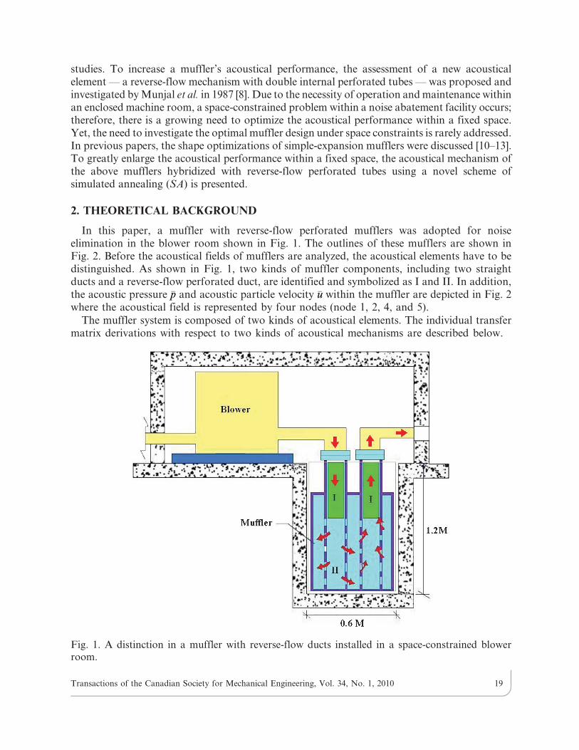
studies. To increase a muffler’s acoustical performance, the assessment of a new acousticalelement — a reverse-flow mechanism with double internal perforated tubes — was proposed andinvestigated by Munjal et al. in 1987 [8]. Due to the necessity of operation and maintenance withinan enclosed machine room, a space-constrained problem within a noise abatement facility occurs;therefore, there is a growing need to optimize the acoustical performance within a fixed space.Yet, the need to investigate the optimal muffler design under space constraints is rarely addressed.In previous papers, the shape optimizations of simple-expansion mufflers were discussed [10–13].To greatly enlarge the acoustical performance within a fixed space, the acoustical mechanism ofthe above mufflers hybridized with reverse-flow perforated tubes using a novel scheme ofsimulated annealing (SA) is presented.

2. THEORETICAL BACKGROUND

In this paper, a muffler with reverse-flow perforated mufflers was adopted for noiseelimination in the blower room shown in Fig. 1. The outlines of these mufflers are shown inFig. 2. Before the acoustical fields of mufflers are analyzed, the acoustical elements have to bedistinguished. As shown in Fig. 1, two kinds of muffler components, including two straightducts and a reverse-flow perforated duct, are identified and symbolized as I and II. In addition,the acoustic pressure �pp and acoustic particle velocity �uu within the muffler are depicted in Fig. 2where the acoustical field is represented by four nodes (node 1, 2, 4, and 5).

The muffler system is composed of two kinds of acoustical elements. The individual transfermatrix derivations with respect to two kinds of acoustical mechanisms are described below.

Fig. 1. A distinction in a muffler with reverse-flow ducts installed in a space-constrained blowerroom.


2.1. System MatrixBased on plane wave theory, the four-pole transfer matrix for a straight duct between nodes 1

and 2 is [14]

�pp1

roco�uu1

� �~e

{jM1kL1

1{M21

TS11,1 TS11,2

TS12,1 TS12,2

� ��pp2

roco�uu2

� �ð1aÞ

where

TS11,1~cosk(L1zLA)

1{M21

� �; TS11,2~j sin

k(L1zLA)

1{M21

� �; TS12,1~j sin

k(L1zLA)

1{M21

� �;

TS12,2~cosk(L1zLA)

1{M21

� � ð1bÞ

Similarly, the relationship between nodes 4 and 5 is

�pp4

roco�uu4

� �~e

{jM4k(L1zLA)

1{M24

TS31,1 TS31,2

TS32,1 TS32,2

� ��pp5

roco�uu5

� �ð2aÞ

where

TS31,1~cosk L1zLAð Þ

1{M24

� �; TS31,2~j sin

k L1zLAð Þ1{M2

4

� �; TS32,1~j sin

k L1zLAð Þ1{M2

4

� �;

TS32,2~cosk L1zLAð Þ

1{M24

� � ð2bÞ

As derived in Appendix A, on the basis of plane wave theory, the four-pole transfer matrixfor a reverse-flow perforated duct between nodes 2 and 4 is

Fig. 2. The outline and acoustical field of a muffler with reverse-flow ducts.


�pp2

roco�uu2

� �~

TPRF21,1 TPRF21,2

TPRF22,1 TPRF22,2

� ��pp4

roco�uu4

� �ð3Þ

The total transfer matrix assembled by multiplication from Eqs. (1),(3) is

�pp1

roco�uu1

!

~e{jk

M1 L1zLAð Þ1{M2

1

zM4 L1zLAð Þ

1{M24

� �TS11,1 TS11,2

TS12,1 TS12,2

" #TPFR21,1 TPRF21,2

TPRF22,1 TPRF22,2

" #

TS31,1 TS31,2

TS32,1 TS32,2

" #�pp5

roco�uu5

!ð4Þ

A simplified form in the matrix is expressed as

�pp1

roco�uu1

� �~

T�11 T�12

T�21 T�22

� ��pp5

roco�uu5

� �ð5Þ

Under the assumption of a fixed thickness of the tubes (t15t250.001 m) and the symmetricdesign (LA5LB5(LZ-LC)/2), the sound transmission loss (STL) of a muffler is definedas [14]

STL Q, f , RT1, RT2, RT3, RT4, dh1, g1, dh2, g2ð Þ

~logT�11zT�12zT�21zT�22

�� 2

� �z10 log

S1

S5

� � ð6aÞ

where

RT1~ LZ=Lo; RT2~ LC=LZ; RT3~ D1=Do; RT4~ D2=Do;

Lo~L1zLZ; LZ~LAzLBzLC; LA~LB~ LZ{LCð Þ=2ð6bÞ

2.2. Overall Sound Power LevelThe silenced octave sound power level emitted from a silencer’s outlet is

SWLi~SWLOi{STLi ð7Þ

where (1) SWLOi is the original SWL at the inlet of a muffler (or pipe outlet), and i is the indexof the octave band frequency.

(2) STLi is the muffler’s STL with respect to the relative octave band frequency.

(3) SWLi is the silenced SWL at the outlet of a muffler with respect to the relative octaveband frequency.


Finally, the overall SWLT silenced by a muffler at the outlet is

SWLT~10 � logX6

i~1

10SWLi=10

( )

~10 � log

10SWLO f ~125ð Þ{½

STL f ~125ð Þ�=10 z10½SWLO f ~250ð Þ{STL f ~250ð Þ�=10 z10

SWLO f ~500ð Þ{½STL f ~500ð Þ�=10

z10SWLO f ~1000ð Þ{½

STL f ~1000ð Þ�=10 z10SWLO f ~2000ð Þ{½

STL f ~2000ð Þ�=10

z10 SWL f ~4000ð Þ{STL f ~4000ð Þ½ �=10

8>>>><>>>>:

9>>>>=>>>>;

ð8Þ

2.3. Objective FunctionBy using the formulas of Eqs. (6) and (8), the objective function used in the SA optimization

was established.

STL Maximization for a One-tone (f) Noise:

OBJ1~STL Q,f ,RT1,RT2,RT3,RT4,dh1,g1,dh2,g2ð Þ ð9Þ

SWL Minimization for a Broadband Noise:To minimize the overall SWLT, the objective function is

OBJ2~SWLT Q,RT1,RT2,RT3,RT4,dh1,g1,dh2,g2ð Þ ð10Þ

3. MODEL CHECK

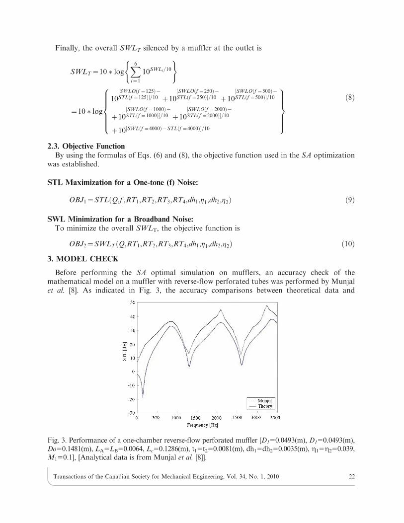
Before performing the SA optimal simulation on mufflers, an accuracy check of themathematical model on a muffler with reverse-flow perforated tubes was performed by Munjalet al. [8]. As indicated in Fig. 3, the accuracy comparisons between theoretical data and

Fig. 3. Performance of a one-chamber reverse-flow perforated muffler [D150.0493(m), D150.0493(m),Do50.1481(m), LA5LB50.0064, Lc50.1286(m), t15t250.0081(m), dh15dh250.0035(m), g15g250.039,M150.1], [Analytical data is from Munjal et al. [8]].


analytical data are in agreement. Therefore, the mathematic model of mufflers with reverse-flowand perforated tubes is acceptable and adopted in the following optimization process.

4. CASE STUDIES

In this paper, the noise reduction of a space-constrained blower is exemplified and shown inFig. 1. The sound power level (SWL) inside the blower’s outlet is shown in Table 1 where theoverall SWL reaches 140.7 dB. To depress the huge exhaust noise emitted from the blower’soutlet, a muffler hybridized with reverse-flow tubes installed under the ground is considered.

To obtain the best acoustical performance within a fixed space volume, numerical assessmentslinked to a SA optimizer are applied. Before the minimization of a broadband noise is executed, areliability check of the SA method by maximization of the STL at one targeted tone (300 Hz) hasbeen carried out. As shown in Figs. 1 and 2, the available space for a muffler is 0.6 m in width,0.6 m in height, and 1.2 m in length. The flow rate (Q) and thickness of a perforated tube (t) arepreset as 0.05 (m3/s) and 0.001(m), respectively. The corresponding OBJ functions, spaceconstraints, and the ranges of design parameters are summarized in Table 2.

5. SIMULATED ANNEALING

The basic concept behind SA was first introduced by Metropolis et al. [15] and developed byKirkpatrick et al. [16]. SA simulates the annealing of metal. Annealing is the process of heatingand keeping a metal at a stabilized temperature while cooling it slowly. Slow cooling allows theparticles to attain their state close to the minimal energy state. The algorithm starts bygenerating a random initial solution. The scheme of the SA is a variation of the hill-climbingalgorithm. All downhill movements for improvement are accepted for the decrement of thesystem’s energy. The purpose of SA is to avoid stacking in local optimal solutions duringoptimization. In order to escape from the local optimum, the SA also allows movementsresulting in solutions that are worse (uphill moves) than the current solution. To imitate theevolution of the SA algorithm, a new random solution (X’) is chosen from the neighborhood ofthe current solution (X). If the change in objective function (or energy) is negative (DFƒ0), thenew solution will be accepted as the new current solution with the transition property pb(X’) 5

1. If the change is not negative (DFw0), the new transition property pb(X’) will be computedby the Boltzmann’s factor pb(X’) 5 exp DF=CTð Þ as the Eq. (11)

Table 1. The spectrum of exhaust sound power levels (SWLs).

f(Hz) 125 250 500 1k 2k 4k OverallSWLO-dB 130 140 128 115 110 105 140.7

Table 2. Range of design parameters for a muffler with reverse-flow ducts.

Range of design parameters

A muffler withreverse-flow ducts

Targeted f 5300 (Hz); Q50.05 (m3/s); Lo51.2 (m); Do50.6 (m)RT1:[0.5, 0.9]; RT2:[0.1, 0.9]; RT3:[0.1, 0.4]; RT4:[0.1, 0.4]; g1:[0. 03, 0.1]; dh1:[0. 00175, 0.007]; g2:[0. 03, 0.1]; dh2:[0. 00175,0.007];


pb X 0ð Þ~1,DFƒ0

exp{DF

CT

� �,Df w0

0@ ð11aÞ

DF~F X 0ð Þ{F Xð Þ ð11bÞwhere C and T are the Boltzmann constant and the current temperature. Moreover, comparedwith the new random probability of rand(0,1), each successful substitution of the new currentsolution will lead to the decay of the current temperature as

Tnew ~ kk � Told

where kk is the cooling rate. The process is repeated until the predetermined number (Iter) ofthe outer loop is reached.

The flow diagram of the SA optimization is described and shown in Fig. 4.

6. RESULTS AND DISCUSSION

6.1. ResultsThe accuracy of the SA optimization depends on the cooling rate (kk) and the number of

iterations (Iter). To achieve good optimization, both the cooling rate (kk) and the number ofiterations (Iter) are varied step by step

Fig. 4. Flow diagram of a SA optimization.


kk ~ 0:90,0:93,0:96,0:99ð Þ; Iter ~ 50,200,800ð Þ

The results of two kinds of optimizations — one of the pure tone noise and the others of thebroadband noise — are described below.

Pure Tone Noise Optimization:Six sets of SA parameters are tested by varying the values of the SA parameters. The

simulated results with respect to the pure tone of 300 Hz is summarized and shown inTable 3. As indicated in Table 3, the optimal design data can be obtained from the last setof SA parameters at (kk, Iter) 5 (0.99, 800). Using the optimal design in a theoreticalcalculation, the optimal STL curves with respect to various SA parameters are plotted anddepicted in Fig. 5. As revealed in Fig. 5, the optimal STL is maximized at the desiredfrequency.

Table 3. Optimal STL for a muffler with reverse-flow ducts (at a targeted tone of 300 Hz).

SA parameters Results

kk Iter

0.90 50 RT1 RT2 RT3 RT4 STL (dB)0.8997 0.8993 0.3997 0.3997 19.5g1 dh1(m) g2 dh2(m)0.006996 0.09994 0.006996 0.09994






Notes: RT15 LZ/Lo; RT25 LC/LZ; RT 35 D1/Do; RT45 D2/Do; Lo5L1+LZ; LZ5 LA+LB+LC; LA5LB5

(LZ-LC)/2.


Broadband Noise Optimization:By using the above SA parameters, the muffler’s optimal design data for mufflers hybridized

with reverse-flow perforated ducts used to minimize the sound power level at the muffler’soutlet is summarized in Table 4. As illustrated in Table 4, the resultant sound power levels havebeen dramatically reduced from 140.7 dB to 42.5 dB. Using this optimal design in a theoreticalcalculation, the resultant SWL before and after adding the muffler at the outlet is shown inFig. 6. As shown in Fig. 6, the muffler has the best acoustical performance.

6.2. DiscussionTo achieve a sufficient optimization, the selection of the appropriate SA parameter set is

essential. As indicated in Table 3, the best SA set at the targeted pure tone noise of 300 Hz has

Fig. 5. The STL with respect to frequencies at various SA parameters (targeted tone: 300Hz).

Table 4. Optimal SWL for a muffler with reverse-flow ducts (broadband noise).

ItemSA parameters Results

kk Iter

1 0.99 50 RT1 RT2 RT3 RT4 SWLT (dB)0.8227 0.7453 0.3420 0.3420 75.5g1 dh1(m) g2 dh2(m)0.005985 0.08647 0.005985 0.08647




been shown. Using the appropriate SA set at the targeted pure tone (300 Hz), the related optimalSTL curves plotted in Fig. 5 reveals that the predicted maximal value of the STL is located at thedesired frequency. Therefore, using the SA optimization in finding a better design solution hasproven reliable; moreover, as can be seen in Fig. 5, not only the peak frequency of the STL profileis shifting toward the targeted tone but the peak value will increase when a better solution assessedin the SA optimization procedure. Meanwhile, all of the design data (RT1, RT2, RT3, RT4, g1, dh1,

g2, dh2) were decrease. It means that the shorter of the length of the perforated tube and thesmaller diameter and number of the perforated hole will result in a higher frequency. Besides, theSTL will also increase when the diameter of the perforated tubes decrease.

7. CONCLUSION

It has been shown that mufflers hybridized with reversed-flow and perforated ducts can beeasily and efficiently optimized within a limited space by using a generalized decouplingtechnique, a plane wave theory, a four-pole transfer matrix, as well as a SA optimizer. Two kindsof SA parameters (kk, Iter) play essential roles in the solution’s accuracy during the SA

optimization. As indicated in Fig. 5, the tuning ability established by adjusting design of themufflers is reliable. In additional, the design data reveals that the peak frequency of the STL willshift rightward if the length of the perforated tube, the diameter of the perforated hole, and thenumber of the perforated hole decrease. Besides, the whole STL will increase if the diameter of theperforated tubes decreases. Subsequently, the appropriate acoustical performance curve ofmufflers with reverse-flow and perforated ducts in depressing overall broadband noise have beenassessed. As can be seen in Table 4 and Fig. 6, the overall sound power level (SWLT) of a blower isminimized by adjusting an appropriate spectrum of the STL. Consequently, the approach usedfor the optimal design of the STL proposed in this study is indeed easy and quite effective.

ACKNOWLEDGEMENTS

The author acknowledges the financial support of the National Science Council (NSC 97-2622-E-235-002-CC3, Taiwan, ROC) and would also like to thank the anonymous referees whokindly provided the suggestions and comments to improve this work.

Fig. 6. Optimal STL for mufflers designed at various SA parameters (broadband noise).


REFERENCES

1. Davis, D.D., Stokes, J.M., Moorse, L., ‘‘Theoretical and experimental investigation of mufflers

with components on engine muffler design,’’ NACA Report, pp.1192, 1954.

2. Sullivan, J.W. and Crocker, M.J., ‘‘Analysis of concentric tube resonators having unpartitioned

cavities,’’ Acoustical Society of America, Vol. 64, pp. 207–215, 1978.

3. Sullivan, J.W., ‘‘A method of modeling perforated tube muffler components I: theory,’’

Acoustical Society of America, Vol. 66, pp. 772–778, 1979.

4. Sullivan, J.W., ‘‘A method of modeling perforated tube muffler components II: theory,’’

Acoustical Society of America, Vol. 66, pp. 779–788, 1979.

5. Jayaraman, K. and Yam, K., ‘‘Decoupling approach to modeling perforated tube muffler

component,’’ Acoustical Society of America, Vol. 69, No. 2, pp. 390–396, 1981.

6. Thawani, P.T. and Jayaraman, K., ‘‘Modeling and applications of straight-through

resonators,’’ Acoustical Society of America, Vol. 73, No. 4, pp. 1387–1389, 1983.

7. Rao, K.N. and Munjal, M.L., ‘‘A Generalized Decoupling Method for Analyzing Perforated

Element Mufflers,’’ Nelson Acoustics Conference, Madison, 1984.

8. Munjal, M.L., Rao, K.N. and Sahasrabudhe, A.D., ‘‘Aeroacoustic analysis of perforatedmuffler components,’’ Journal of Sound and Vibration, Vol. 114, No. 2, pp. 173–188, 1987.

9. Peat, K.S., ‘‘A numerical decoupling analysis of perforated pipe silencer elements,’’ Journal of

Sound and Vibration, Vol. 123, No. 2, pp. 199–212, 1988.

10. Yeh, L.J., Chang, Y.C., Chiu, M.C. and Lai, G.J., ‘‘Computer-aided optimal design of a single-

chamber muffler with side inlet/outlet under space constraints,’’ Journal of Marine Science and

Technology, Vol. 11, No. 4, pp. 1–8, 2003.

11. Chang, Y.C., Yeh, L. J. and Chiu, M.C., ‘‘Numerical studies on constrained venting system with

side inlet/outlet mufflers by GA optimization,’’ Acta Acustica united with Acustica, Vol. 90, pp.

1–11, 2004.

12. Chang, Y.C., Yeh, L.J. and Chiu, M.C., ‘‘Shape optimization on double-chamber mufflers

using genetic algorithm,’’ Proc. ImechE Part C: Journal of Mechanical Engineering Science, Vol.

10, pp. 31–42, 2005.

13. Yeh, L.J., Chang, Y.C. and Chiu, M.C., ‘‘Numerical studies on constrained venting system with

reactive mufflers by GA optimization,’’ International Journal for Numerical Methods in

Engineering, Vol. 65, pp. 1165–1185, 2006.

14. Munjal, M.L. ‘‘Acoustics of Ducts and Mufflers with Application to Exhaust and Ventilation

System Design,’’ New York: John Wiley & Sons, 1987.

15. Metropolis, A., Rosenbluth, W., Rosenbluth, M. N., Teller, H. and Teller, E., ‘‘Equation ofstatic calculations by fast computing machines,’’ The Journal of Chemical Physics, Vol. 21, pp.

1087–1092, 1953.

16. Kirkpatrick, S., Gelatt, C.D. and Vecchi, M.P., ‘‘Optimization by simulated annealing,’’

Science, Vol. 220, pp. 671–680, 1983.

17. Rao, K.N. and Munjal, M.L., ‘‘Experimental evaluation of impedance of perforates with

grazing flow,’’ Journal of Sound and Vibration, Vol. 123, pp. 283–295, 1986.


APPENDIX A-TRANSFER MATRIX OF A REVERSE-FLOW PERFORATED DUCT

As shown in Fig. 7, there are six nodes located inside the acoustical field. Based on thederivation from Munjal et al. [14], the continuity equations and momentum equations withrespect to the inner and outer tubes in the first chamber are listed below.

Inner tube 1:

continuity equation

V2Lr2

Lxzro

Lu2

Lxz

4ro

D1u2,3z

Lr2

Lt~0 ðA1Þ

momentum equation

ro

LLt

zV2LLx

� �u2z

Lp2

Lx~0 ðA2Þ

Inner tube 2:

continuity equation

V4Lr4

Lxzro

Lu4

Lx{

4ro

D8u3,4z

Lr4

Lt~0 ðA3Þ

momentum equation

ro

LLt

zV4LLx

� �u4z

Lp4

Lx~0 ðA4Þ

Outer tube:

continuity equation

ro

Lu3

Lx{V3

Lr3

Lx{

4D1ro

D2o{D2

1{D22

u2,3z4D2

D2o{D2

1{D22

rou2,3zLr3

Lt~0 ðA5Þ

momentum equation

Fig. 7. The mechanism of an acoustical element for a muffler with reverse -flow perforated ducts.


ro

LLt

zV3LLx

� �u3z

Lr3

Lx~0 ðA6Þ

Assuming that the acoustic wave is a harmonic motion

p x,tð Þ~P xð Þ:ejvt ðA7Þ

under the isentropic processes in ducts, it yields

P xð Þ~r xð Þ:c2o ðA8Þ

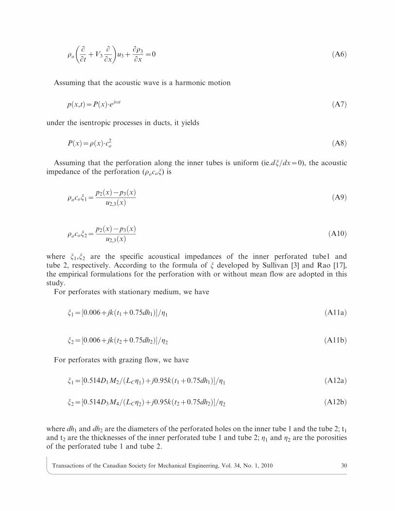
Assuming that the perforation along the inner tubes is uniform (ie.dj=dx~0), the acousticimpedance of the perforation (rocoj) is

rocoj1~p2 xð Þ{p3 xð Þ

u2,3 xð Þ ðA9Þ

rocoj2~p2 xð Þ{p3 xð Þ

u2,3 xð Þ ðA10Þ

where j1,j2 are the specific acoustical impedances of the inner perforated tube1 andtube 2, respectively. According to the formula of j developed by Sullivan [3] and Rao [17],the empirical formulations for the perforation with or without mean flow are adopted in thisstudy.

For perforates with stationary medium, we have

j1~ 0:006zjk t1z0:75dh1ð Þ½ �=g1 ðA11aÞ

j2~ 0:006zjk t2z0:75dh2ð Þ½ �=g2 ðA11bÞ

For perforates with grazing flow, we have

j1~ 0:514D1M2= LCg1ð Þzj0:95k t1z0:75dh1ð Þ½ �=g1 ðA12aÞ

j2~ 0:514D3M4= LCg2ð Þzj0:95k t2z0:75dh2ð Þ½ �=g2 ðA12bÞ

where dh1 and dh2 are the diameters of the perforated holes on the inner tube 1 and the tube 2; t1

and t2 are the thicknesses of the inner perforated tube 1 and tube 2; g1 and g2 are the porositiesof the perforated tube 1 and tube 2.


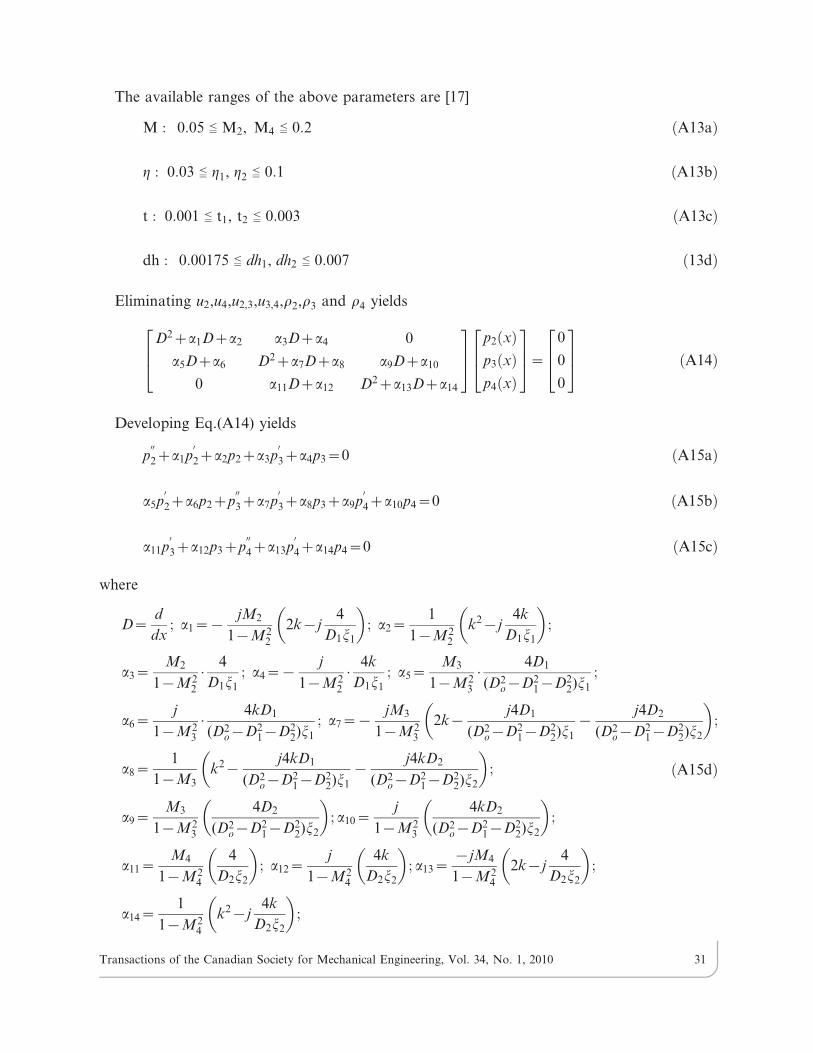
The available ranges of the above parameters are [17]

M : 0:05 ¼v M2, M4 ¼v 0:2 ðA13aÞ

g : 0:03 ¼v g1, g2 ¼v 0:1 ðA13bÞ

t : 0:001 ¼v t1, t2 ¼v 0:003 ðA13cÞ

dh : 0:00175 ¼v dh1, dh2 ¼v 0:007 ð13dÞ

Eliminating u2,u4,u2,3,u3,4,r2,r3 and r4 yields

D2za1Dza2 a3Dza4 0

a5Dza6 D2za7Dza8 a9Dza10

0 a11Dza12 D2za13Dza14

264

375

p2 xð Þp3 xð Þp4 xð Þ

264

375~

0

0

0

264375 ðA14Þ

Developing Eq.(A14) yields

p00

2za1p0

2za2p2za3p0

3za4p3~0 ðA15aÞ

a5p0

2za6p2zp00

3za7p0

3za8p3za9p0

4za10p4~0 ðA15bÞ

a11p0

3za12p3zp00

4za13p0

4za14p4~0 ðA15cÞ

where

D~d

dx; a1~{

jM2

1{M22

2k{j4

D1j1

� �; a2~

1

1{M22

k2{j4k

D1j1

� �;

a3~M2

1{M22

: 4

D1j1

; a4~{j

1{M22

: 4k

D1j1

; a5~M3

1{M23

: 4D1

(D2o{D2

1{D22)j1

;

a6~j

1{M23

: 4kD1

(D2o{D2

1{D22)j1

; a7~{jM3

1{M23

2k{j4D1

(D2o{D2

1{D22)j1

{j4D2

(D2o{D2

1{D22)j2

� �;

a8~1

1{M3k2{

j4kD1

(D2o{D2

1{D22)j1

{j4kD2

(D2o{D2

1{D22)j2

� �;

a9~M3

1{M23

4D2

(D2o{D2

1{D22)j2

� �; a10~

j

1{M23

4kD2

(D2o{D2

1{D22)j2

� �;

a11~M4

1{M24

4

D2j2

� �; a12~

j

1{M24

4k

D2j2

� �; a13~

{jM4

1{M24

2k{j4

D2j2

� �;

a14~1

1{M24

k2{j4k

D2j2

� �;

ðA15dÞ


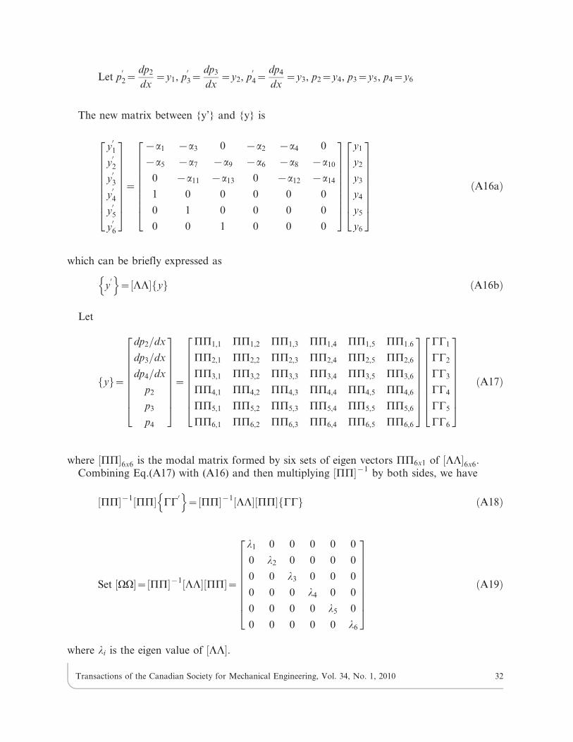
Let p0

2~dp2

dx~y1, p

0

3~dp3

dx~y2, p

0

4~dp4

dx~y3, p2~y4, p3~y5, p4~y6

The new matrix between {y’} and {y} is

y0

1

y0

2

y0

3

y0

4

y05

y0

6

2666666664

3777777775~

{a1 {a3 0 {a2 {a4 0

{a5 {a7 {a9 {a6 {a8 {a10

0 {a11 {a13 0 {a12 {a14

1 0 0 0 0 0

0 1 0 0 0 0

0 0 1 0 0 0

2666666664

3777777775

y1

y2

y3

y4

y5

y6

2666666664

3777777775

ðA16aÞ

which can be briefly expressed as

y0

n o~ LL½ � yf g ðA16bÞ

Let

yf g~

dp2=dx

dp3=dx

dp4=dx

p2

p3

p4

2666666664

3777777775~

PP1,1 PP1,2 PP1,3 PP1,4 PP1,5 PP1:6

PP2,1 PP2,2 PP2,3 PP2,4 PP2,5 PP2,6

PP3,1 PP3,2 PP3,3 PP3,4 PP3,5 PP3,6

PP4,1 PP4,2 PP4,3 PP4,4 PP4,5 PP4,6

PP5,1 PP5,2 PP5,3 PP5,4 PP5,5 PP5,6

PP6,1 PP6,2 PP6,3 PP6,4 PP6,5 PP6,6

2666666664

3777777775

CC1

CC2

CC3

CC4

CC5

CC6

2666666664

3777777775

ðA17Þ

where PP½ �6x6 is the modal matrix formed by six sets of eigen vectors PP6x1 of LL½ �6x6.

Combining Eq.(A17) with (A16) and then multiplying PP½ �{1by both sides, we have

PP½ �{1 PP½ � CC0

n o~ PP½ �{1 LL½ � PP½ � CCf g ðA18Þ

Set VV½ �~ PP½ �{1 LL½ � PP½ �~

l1 0 0 0 0 0

0 l2 0 0 0 0

0 0 l3 0 0 0

0 0 0 l4 0 0

0 0 0 0 l5 0

0 0 0 0 0 l6

2666666664

3777777775

ðA19Þ

where li is the eigen value of LL½ �.


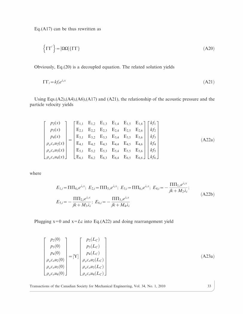
Eq.(A17) can be thus rewritten as

CC0

n o~ VV½ � CCf g ðA20Þ

Obviously, Eq.(20) is a decoupled equation. The related solution yields

CCi~kfielix ðA21Þ

Using Eqs.(A2),(A4),(A6),(A17) and (A21), the relationship of the acoustic pressure and theparticle velocity yields

p2(x)

p3(x)

p4(x)

rocou2(x)

rocou3(x)

rocou4(x)

2666666664

3777777775~

E1,1 E1,2 E1,3 E1,4 E1,5 E1,6

E2,1 E2,2 E2,3 E2,4 E2,5 E2,6

E3,1 E3,2 E3,3 E3,4 E3,5 E3,6

E4,1 E4,2 E4,3 E4,4 E4,5 E4,6

E5,1 E5,2 E5,3 E5,4 E5,5 E5,6

E6,1 E6,2 E6,3 E6,4 E6,5 E6,6

2666666664

3777777775

kf1

kf2

kf3

kf4

kf5

kf6

2666666664

3777777775

ðA22aÞ

where

E1,i~PP4,ielix; E2,i~PP5,ie

lix; E3,i~PP6,ielix; E4,i~{

PP1,ielix

jkzM2li

;

E5,i~{PP2,ie

lix

jkzM3li

; E6,i~{PP3,ie

lix

jkzM4li

ðA22bÞ

Plugging x50 and x5Lc into Eq.(A22) and doing rearrangement yield

p2 0ð Þp3 0ð Þp4 0ð Þ

rocou2 0ð Þrocou3 0ð Þrocou4 0ð Þ

2666666664

3777777775~ Y½ �

p2 LCð Þp3 LCð Þp4 LCð Þ

rocou2 LCð Þrocou3 LCð Þrocou4 LCð Þ

2666666664

3777777775

ðA23aÞ


where

Y½ �~ E 0ð Þ½ � E LCð Þ½ �{1 ðA23bÞ

To obtain the transform matrix between the inlet (x50) and the outlet (x5Lc) of the innertubes, four boundary conditions for the outer tube at x50 and x5Lc are placed in thecalculation.

p3 0ð Þ{u3 0ð Þ~{jroco cot kLAð Þ ðA24aÞ

p2 LCð Þu2 LCð Þ~{jroco cot kLBð Þ ðA24bÞ

p3 LCð Þu3 LCð Þ~{jroco cot kLBð Þ ðA24cÞ

p4 LCð Þu4 LCð Þ~{jroco cot kLBð Þ ðA24dÞ

By combining Eqs.(A23a, b, c, d) with Eq.(A24) and developing them, the transfer matrixyields

p2 0ð Þrocou2 0ð Þ

� �~

TPRF21,1 TPRF21,2

TPRF22,1 TPRF22,2

� �p4 LCð Þ

rocou4 LCð Þ

� �ðA25aÞ

or in a brief form

�pp2

roco�uu2

� �~

TPRF21,1 TPRF21,2

TPRF22,1 TPRF22,2

� ��pp4

roco�uu4

� �ðA25bÞ


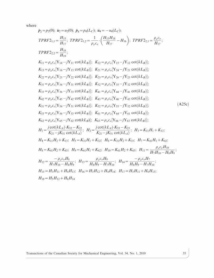
where�pp2~p2(0); �uu2~u2(0); �pp4~p4(LC); �uu4~{u4(LC);

TPRF21,1~H15

H17; TPRF21,2~

1

roco

: H15H18

H17{H16

� �; TPRF22,1~

roco

H17;

TPRF22,2~H18

H19;

K11~roco Y14{jY11 cot kLBð Þ½ �; K12~roco Y15{jY12 cot kLBð Þ½ �;








K62~roco Y65{jY62 cot(kLB)½ �; K63~roco Y66{jY63 cot kLBð Þ½ �;

H1~j cot kLAð Þ:K52{K22

K21{jK51 cot kLAð Þ ; H2~j cot kLAð Þ:K53{K23

K21{jK51 cot kLAð Þ ; H3~K11H1zK12;

H4~K11H2zK13; H5~K31H1zK32; H6~K31H2zK33; H7~K41H1zK42;

H8~K41H2zK43; H9~K61H1zK62; H10~K61H2zK63; H11~rocoH10

H7H10{H8H9;

H12~{rocoH8

H7H10{H8H9; H13~

rocoH9

H8H9{H7H10; H14~

{rocoH7

H8H9{H7H10;

H15~H3H11zH4H13; H16~H3H12zH4H14; H17~H5H11zH6H13;

H18~H5H12zH6H14

ðA25cÞ


numerical assessment of reverse-flow mufflers using a...

Documents