numerical methodsfyzikazeme.sk/mainpage/stud_mat/nm/lecture2.pdf · bisection method bisection...
TRANSCRIPT

Lecture 2
Numerical methodsSolving nonlinear equations
Lecture 2
CONTENTS
1. Introduction2. Root separation and estimation of initial approximation3. Bisection method4. Rate of convergence5. Regula falsi (false position) method6. Secant method7. Newton’s (Newton-Raphson) method8. Steffensen’s method9. Fixed-point iteration10. Aitken Extrapolation11. A few notes12. Literature

Introduction
Solving nonlinear equationf (x)=0
means to find such points thatf (x*)=0.
We call such point roots of function f (x).
In general, we do not know (because it is impossible) the explicit formula for roots of f (x).
Iterative methods:we generate sequence of approximations
from one or several initial approximations (guess)of root x*,
which converge to the root x*.
0 1 2,, ,x x x
*x ÎÂ(1)
Introduction
For some methods it is enoughto prescribe interval ,
which contains the searched root,other require
initial guess to be reasonably close to the true root.
Usually we start with robustbut reliable method
and then, when we are close enough to the root,
we switch to more sophisticated and faster convergent method.
,a b
Introduction
For simplicity, we will consider only problem of findingsimple root x* of function f (x),i.e. we suppose that .
We will also suppose thatfunction f (x) is continuous and
has so many continuous derivatives,how many we need.
( )* 0f x¢ ¹
Lecture 2
CONTENTS
1. Introduction2. Root separation and estimation of initial approximation3. Bisection method4. Rate of convergence5. Regula falsi (false position) method6. Secant method7. Newton’s (Newton-Raphson) method8. Steffensen’s method9. Fixed-point iteration10. Aitken Extrapolation11. A few notes12. Literature
Root separation and estimation of initial approximation
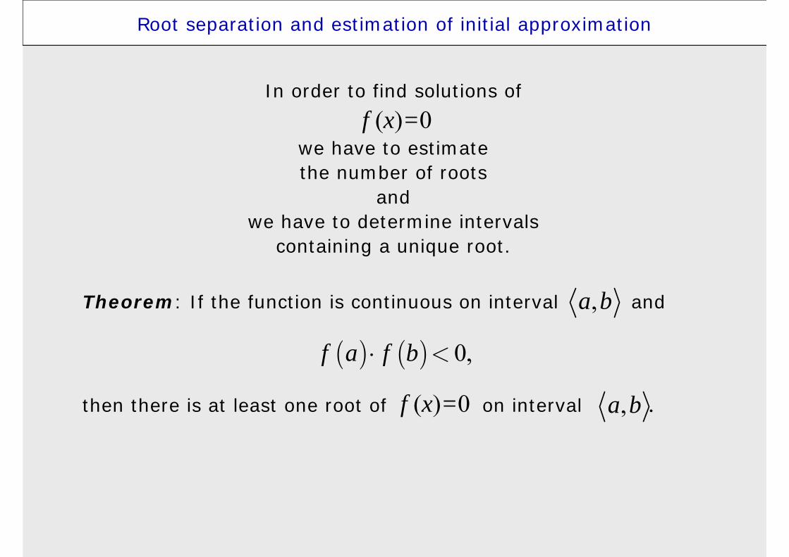
In order to find solutions off (x)=0
we have to estimatethe number of roots
andwe have to determine intervals
containing a unique root.
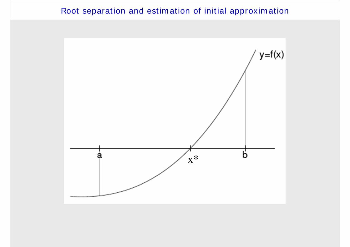
Theorem: If the function is continuous on interval and
then there is at least one root of f (x)=0 on interval .
,a b
,a b
( ) ( ) 0,f a f b⋅ <
Root separation and estimation of initial approximation
x*

Root separation and estimation of initial approximation
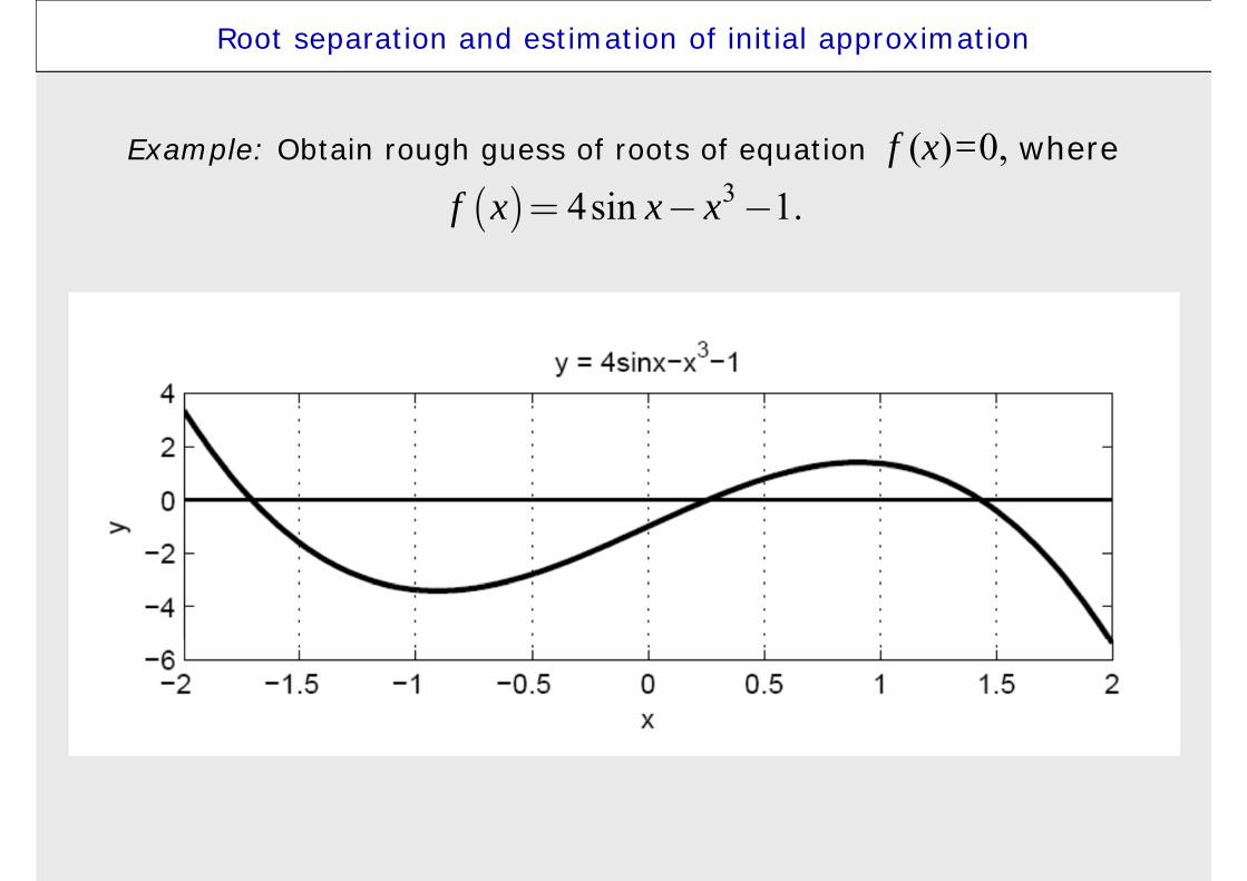
We can find the initial approximation of roots off (x)=0
from graph of function f (x).
,a b
( ),i ix f xé ùë û
0 1 1i i na x x x x x b-= < < < < < < =
Other possibility is to assemble the table of points forsome division
of chosen interval .
Root separation and estimation of initial approximation
Example: Obtain rough guess of roots of equation f (x)=0, where
( ) 34sin 1.f x x x= - -
Root separation and estimation of initial approximation
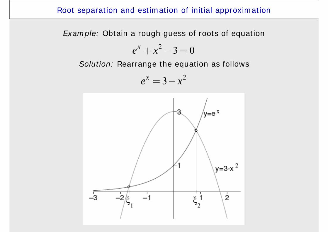
Example: Obtain a rough guess of roots of equation2 3 0xe x+ - =
23xe x= -
Solution: Rearrange the equation as follows
Lecture 2
CONTENTS
1. Introduction2. Root separation and estimation of initial approximation3. Bisection method4. Rate of convergence5. Regula falsi (false position) method6. Secant method7. Newton’s (Newton-Raphson) method8. Steffensen’s method9. Fixed-point iteration10. Aitken Extrapolation11. A few notes12. Literature
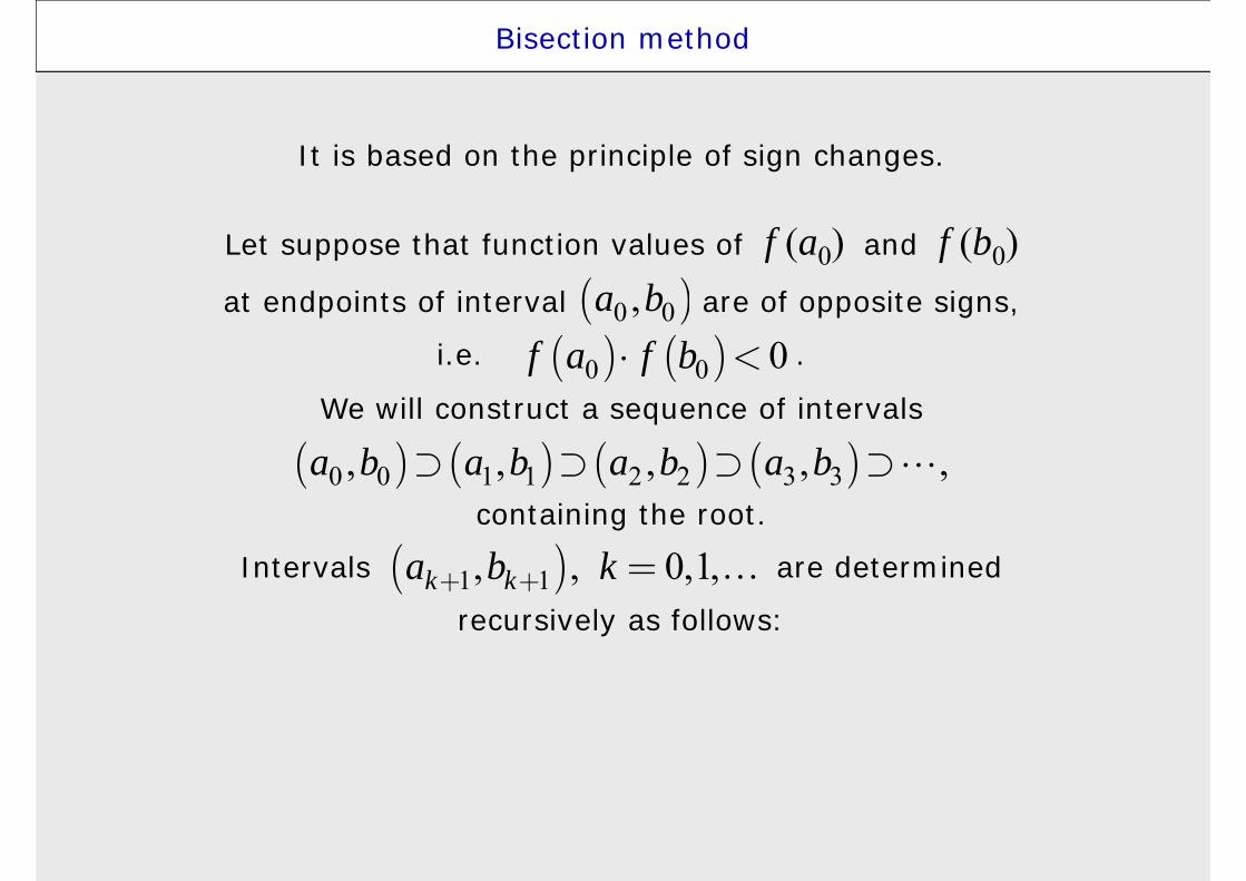
We will construct a sequence of intervals
containing the root.
Intervals are determined
recursively as follows:
Bisection method
Let suppose that function values of f (a0) and f (b0) at endpoints of interval are of opposite signs,
i.e. .
( )0 0,a b( ) ( )0 0 0f a f b⋅ <
It is based on the principle of sign changes.
( ) ( ) ( ) ( )0 0 1 1 2 2 3 3, , , , ,a b a b a b a bÉ É É É
( )1 1, , 0,1,k ka b k+ + =
Bisection method
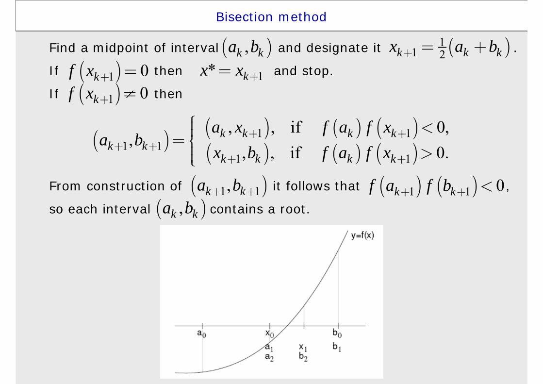
Find a midpoint of interval and designate it .
If then and stop.
If then
From construction of it follows that ,
so each interval contains a root.
( ),k ka b ( )11 2k k kx a b+ = +
( )1 0kf x + =( )1 0kf x + ¹
1* kx x +=
( ) ( ) ( ) ( )( ) ( ) ( )
1 11 1
1 1
, , if 0,,
, , if 0.k k k k
k kk k k k
a x f a f xa b
x b f a f x+ +
+ ++ +
ìï <ï=íï >ïî( )1 1,k ka b+ + ( ) ( )1 1 0k kf a f b+ + <
( ),k ka b
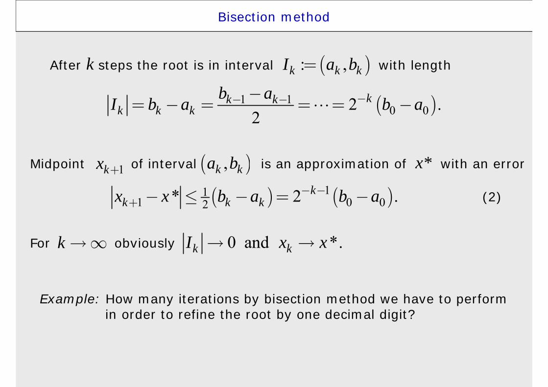
After k steps the root is in interval with length
Bisection method
( ): ,k k kI a b=
( )1 10 02 .
2kk k
k k kb aI b a b a-- --
= - = = = -
Midpoint of interval is an approximation of x* with an error
For obviously
1kx + ( ),k ka b
( ) ( )111 0 02* 2 .k
k k kx x b a b a- -+ - £ - = -
k ¥ 0 and *.k kI x x
(2)
Example: How many iterations by bisection method we have to performin order to refine the root by one decimal digit?
Bisection method
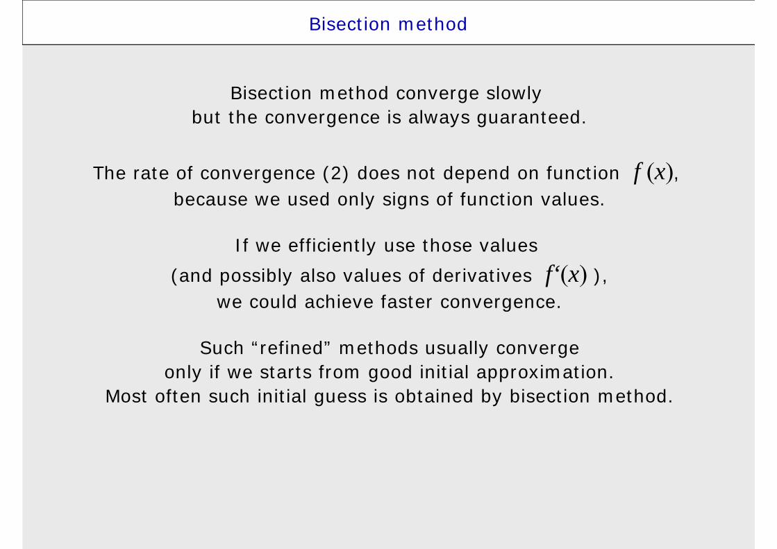
Bisection method converge slowly but the convergence is always guaranteed.
The rate of convergence (2) does not depend on function f (x), because we used only signs of function values.
If we efficiently use those values (and possibly also values of derivatives f‘(x) ),
we could achieve faster convergence.
Such “refined” methods usually convergeonly if we starts from good initial approximation.
Most often such initial guess is obtained by bisection method.

Lecture 2
CONTENTS
1. Introduction2. Root separation and estimation of initial approximation3. Bisection method4. Rate of convergence5. Regula falsi (false position) method6. Secant method7. Newton’s (Newton-Raphson) method8. Steffensen’s method9. Fixed-point iteration10. Aitken Extrapolation11. A few notes12. Literature
Rate of convergence
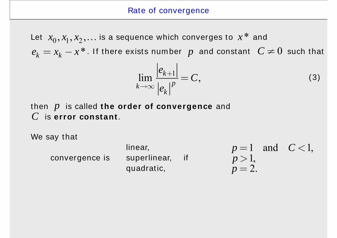
then is called the order of convergence andis error constant.
We say thatlinear,
convergence is superlinear, ifquadratic,
Let is a sequence which converges to and
. If there exists number and constant such that0 1 2, , ,x x x *x
*k ke x x= - p 0C ¹
1lim ,kpk
k
eC
e+
¥=
p
1 and 1,p C= <1,p>2.p =
C
(3)

Rate of convergence
then is called the order of convergence andis error constant.
We say thatlinear,
convergence is superlinear, ifquadratic,
We say that the method converges with order , if all convergent sequences obtained by this methodhave the order of convergence greater or equal to andat least one of them has order of convergence exactly equal to .
Let is a sequence which converges to and
. If there exists number and constant such that0 1 2, , ,x x x *x
*k ke x x= - p 0C ¹
1lim ,kpk
k
eC
e+
¥=
p
1 and 1,p C= <1,p>2.p =
p
pp
C
(3)
Rate of convergence
Example: What is the order of convergence of bisection method?
1lim ,kpk
k
eC
e+
¥= *k ke x x= -
Rate of convergence
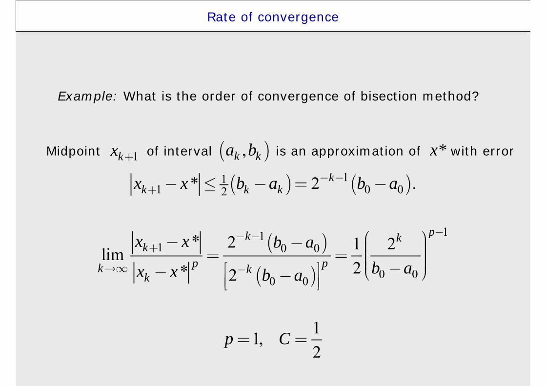
Example: What is the order of convergence of bisection method?
( ) ( )111 0 02* 2 .k
k k kx x b a b a- -+ - £ - = -
Midpoint of interval is an approximation of x* with error1kx + ( ),k ka b
( )
( )
111 0 0
0 00 0
* 2 1 2lim2* 2
pk kk
p pk kk
x x b ab ax x b a
-- -+
¥ -
æ ö- - ÷ç ÷= = ç ÷ç ÷ç -é ù è ø- -ê úë û
11,2
p C= =

Lecture 2
CONTENTS
1. Introduction2. Root separation and estimation of initial approximation3. Bisection method4. Rate of convergence5. Regula falsi (false position) method6. Secant method7. Newton’s (Newton-Raphson) method8. Steffensen’s method9. Fixed-point iteration10. Aitken Extrapolation11. A few notes12. Literature
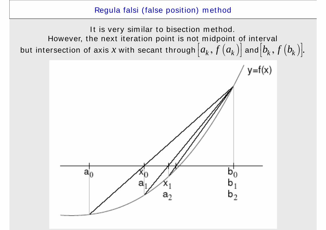
Regula falsi (false position) method
It is very similar to bisection method. However, the next iteration point is not midpoint of interval
but intersection of axis x with secant through and .( ),k ka f aé ùë û ( ),k kb f bé ù
ë û

Regula falsi (false position) method
The root of secant we estimate by
( ) ( )( )1
k kk k k
k k
b ax b f bf b f a+
-= -
-
If then and stop.
If then
From construction of it follows that ,
so each interval contains a root.
( )1 0kf x + =( )1 0kf x + ¹
1* kx x +=
( ) ( ) ( ) ( )( ) ( ) ( )
1 11 1
1 1
, , if 0,,
, , if 0.k k k k
k kk k k k
a x f a f xa b
x b f a f x+ +
+ ++ +
ìï <ï=íï >ïî( )1 1,k ka b+ + ( ) ( )1 1 0k kf a f b+ + <
( ),k ka b
After k steps the root is in interval .
Unlike the bisection method the length of interval in some
cases fail to converge to a zero limit.
Regula falsi (false position) method
Regula falsi method always converges.
The rate of convergence is(similarly as bisection method)
linear.
( ): ,k k kI a b=
kI
Lecture 2
CONTENTS
1. Introduction2. Root separation and estimation of initial approximation3. Bisection method4. Rate of convergence5. Regula falsi (false position) method6. Secant method7. Newton’s (Newton-Raphson) method8. Steffensen’s method9. Fixed-point iteration10. Aitken Extrapolation11. A few notes12. Literature

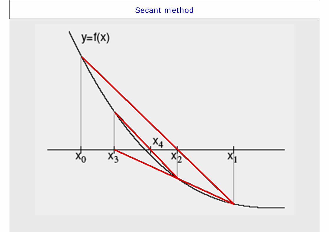
Secant method
It is similar to regula falsi method.
We start from interval containing the root.
Denote and .
Let secant goes through points and and
its intersect with axis xwe denote .
Unlike the regula falsi methodwe will not select an interval containing the root but
we construct secant through points ,and its root we denote .
,a b
0x a= 1x b=
( )0 0,x f xé ùë û ( )1 1,x f xé ùë û
2x
( ) ( )1 1 2 2, , ,x f x x f xé ù é ùë û ë û3x

Secant method
It is similar to regula falsi method.
We start from interval containing the root.
Denote and .
Let secant goes through points and and
its intersect with axis xwe denote .
Unlike the regula falsi methodwe will not select an interval containing the root but
we construct secant through points ,and its root we denote .
Then we construct secant through and and so on.
,a b
0x a= 1x b=
( )0 0,x f xé ùë û ( )1 1,x f xé ùë û
2x
( ) ( )1 1 2 2, , ,x f x x f xé ù é ùë û ë û3x
( )2 2,x f xé ùë û ( )3 3,x f xé ùë û
Secant method
Secant method
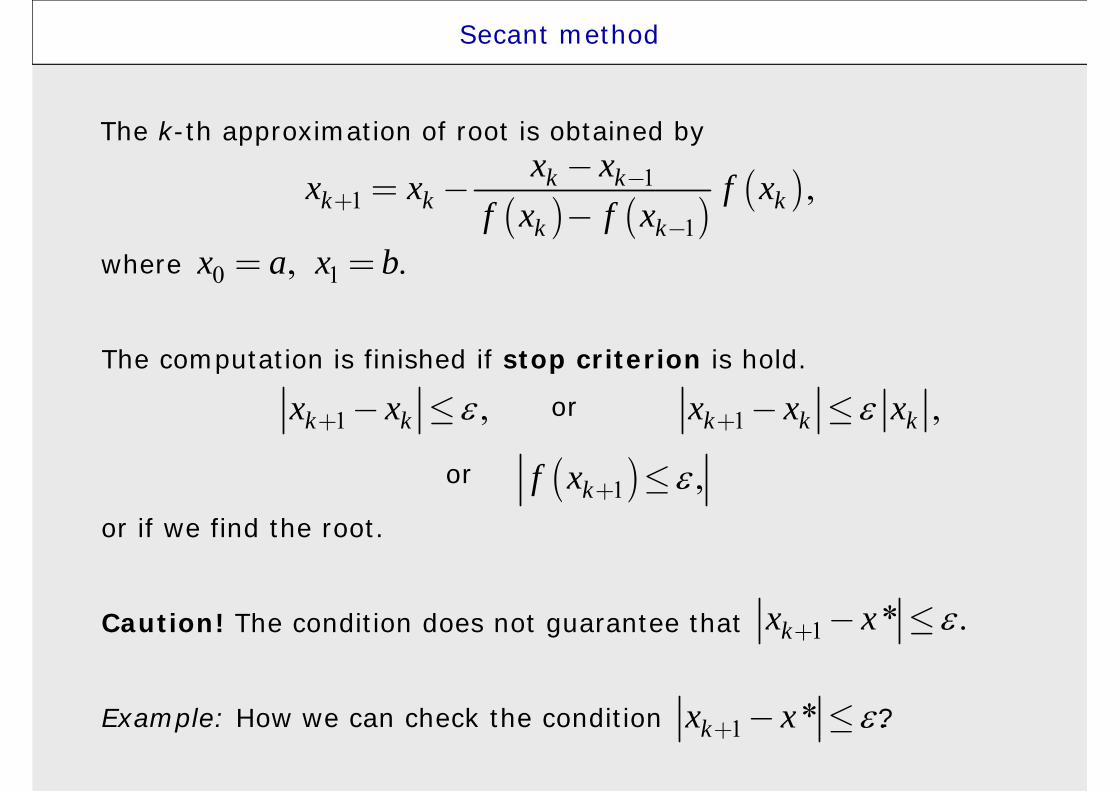
The k-th approximation of root is obtained by
( ) ( )( )1
11
,k kk k k
k k
x xx x f xf x f x
-+
-
-= -
-where
The computation is finished if stop criterion is hold.
or
or
or if we find the root.
Caution! The condition does not guarantee that
Example: How we can check the condition ?
0 1, .x a x b= =
1 ,k kx x + - £
1 * .kx x + - £
1 ,k k kx x x+ - £
( )1 ,kf x + £
1 * .kx x + - £
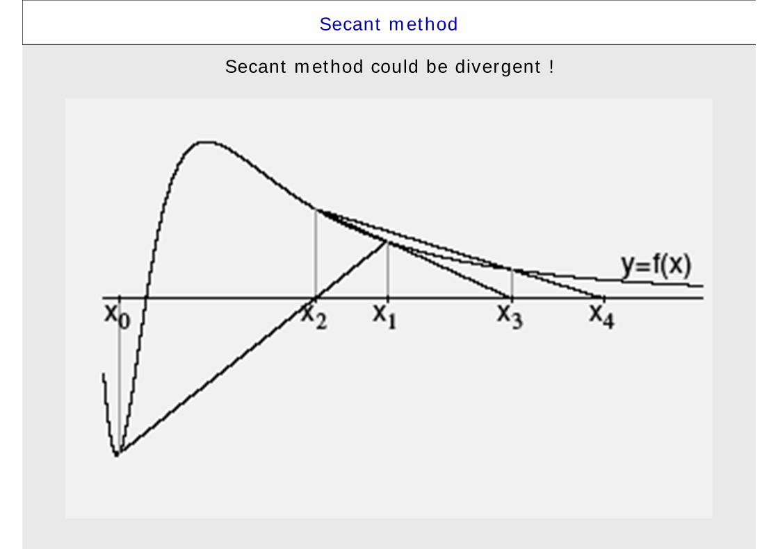
Secant method
Secant method could be divergent !
Secant method
Secant method converge faster than regula falsi,but could also diverge.
It convergeif initial points and are close enough to root .
Is it possible to show, that convergence rate is
i.e. the secant method is superlinear.
1x 2x *x
( )1 1 5 1.618 ,2
p = +

Lecture 2
CONTENTS
1. Introduction2. Root separation and estimation of initial approximation3. Bisection method4. Rate of convergence5. Regula falsi (false position) method6. Secant method7. Newton’s (Newton-Raphson) method8. Steffensen’s method9. Fixed-point iteration10. Aitken Extrapolation11. A few notes12. Literature
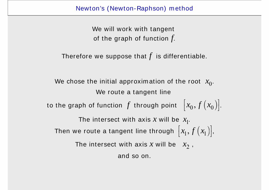
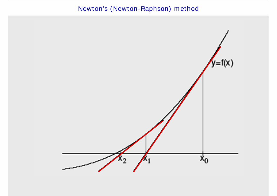
Newton’s (Newton-Raphson) method
We will work with tangent of the graph of function f.
Therefore we suppose that f is differentiable.
We chose the initial approximation of the root .We route a tangent line
to the graph of function f through point .
The intersect with axis x will be .
Then we route a tangent line through ,
The intersect with axis x will be ,
and so on.
0x
( )0 0,x f xé ùë û
1x( )1 1,x f xé ùë û
2x
Newton’s (Newton-Raphson) method
Newton’s (Newton-Raphson) method
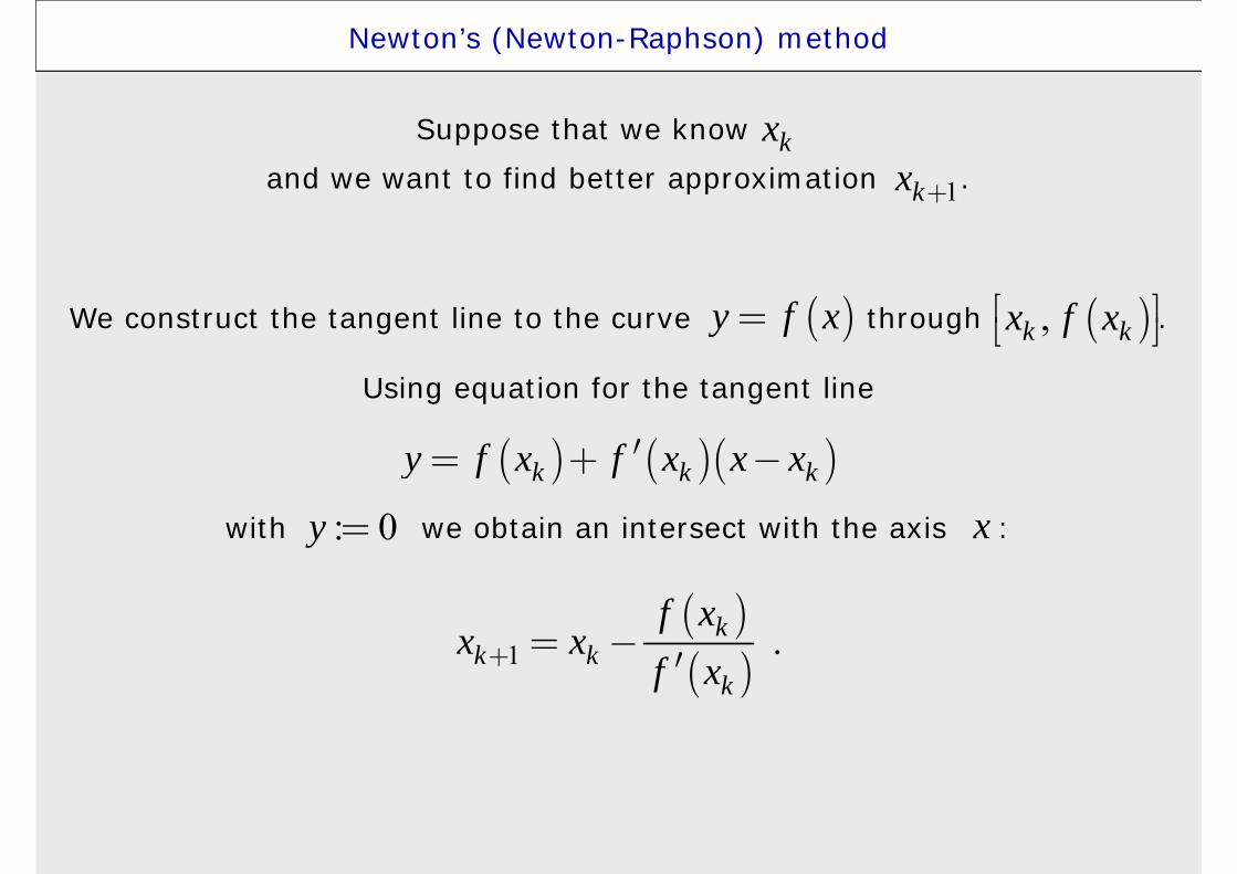
Suppose that we knowand we want to find better approximation .
We construct the tangent line to the curve through .
Using equation for the tangent line
with we obtain an intersect with the axis :
( ),k kx f xé ùë û
kx1kx +
( )y f x=
( ) ( )( )k k ky f x f x x x¢= + -
: 0y = x
( )( )1 .k
k kk
f xx x
f x+ = -¢

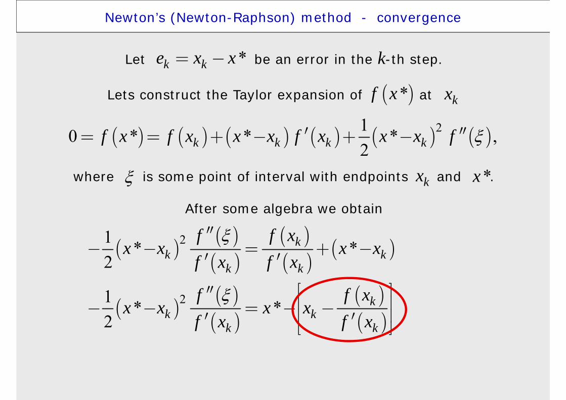
Newton’s (Newton-Raphson) method - convergence
Let be an error in the k-th step.
Lets construct the Taylor expansion of at
where is some point of interval with endpoints and .
After some algebra we obtain
*k ke x x= -
( )*f x kx
( ) ( ) ( ) ( ) ( ) ( )210 * * * ,2k k k kf x f x x x f x x x f ¢ ¢¢= = + - + -
kx *x
( )( )( )
( )( )
( )
( )( )( )
( )( )
( )( )
2
21
21
1 * *2
1 * * *2
12
kk k
k k
kk k k
k k
k kk
f xfx x x x
f x f x
f xfx x x x x x
f x f x
fe e
f x
+
+
¢¢- - = + -
¢ ¢
é ù¢¢ ê ú- - = - - = -ê ú¢ ¢ë û¢¢
=¢
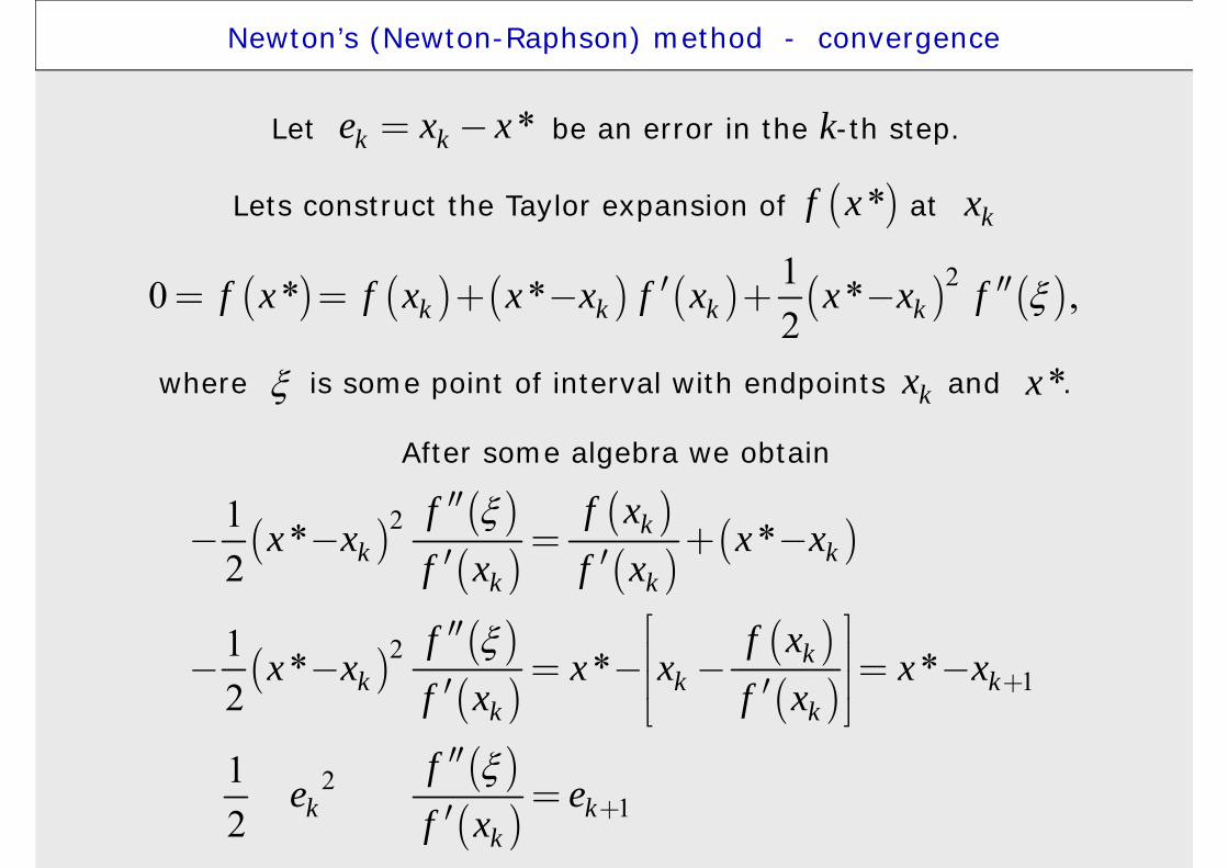
Newton’s (Newton-Raphson) method - convergence
( )( )
21
12 k k
k
fe e
f x
+
¢¢=
¢
( )( )
12lim 2 .k
k kk
fef xe
+
¥
¢¢=
¢
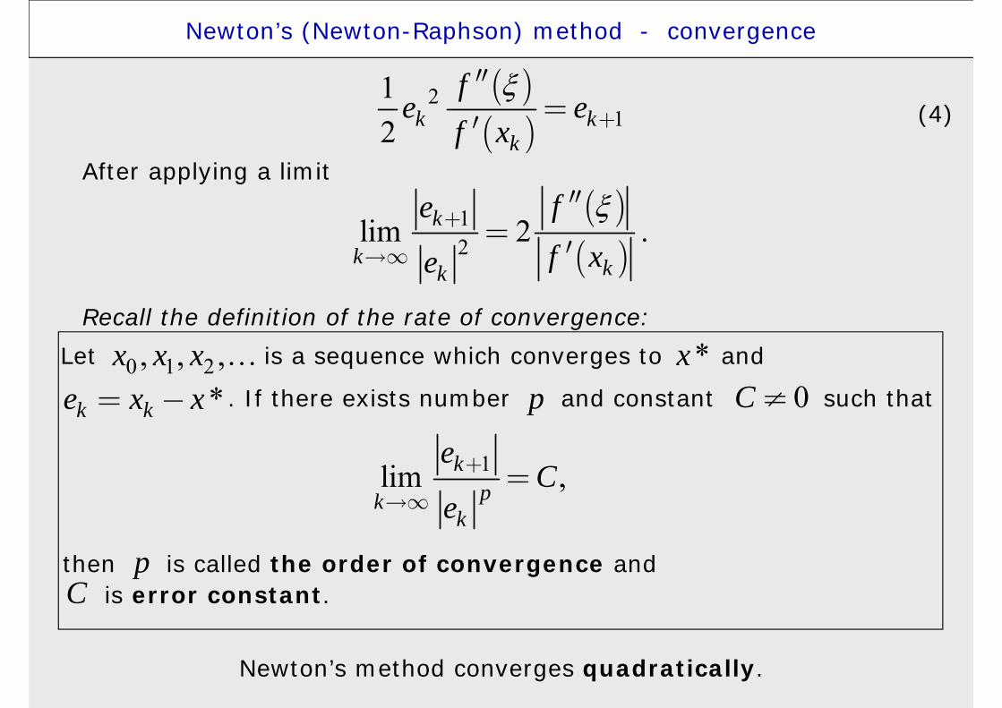
After applying a limit
Newton’s method converges quadratically.
(4)
then is called the order of convergence andis error constant.
pC
Recall the definition of the rate of convergence:Let is a sequence which converges to and
. If there exists number and constant such that0 1 2, , ,x x x *x
*k ke x x= - p 0C ¹
1lim ,kpk
k
eC
e+
¥=
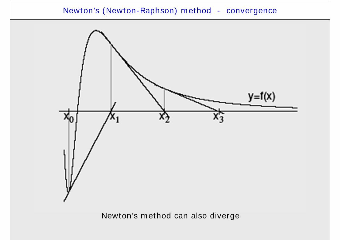
Newton’s (Newton-Raphson) method - convergence
Newton’s method can also diverge
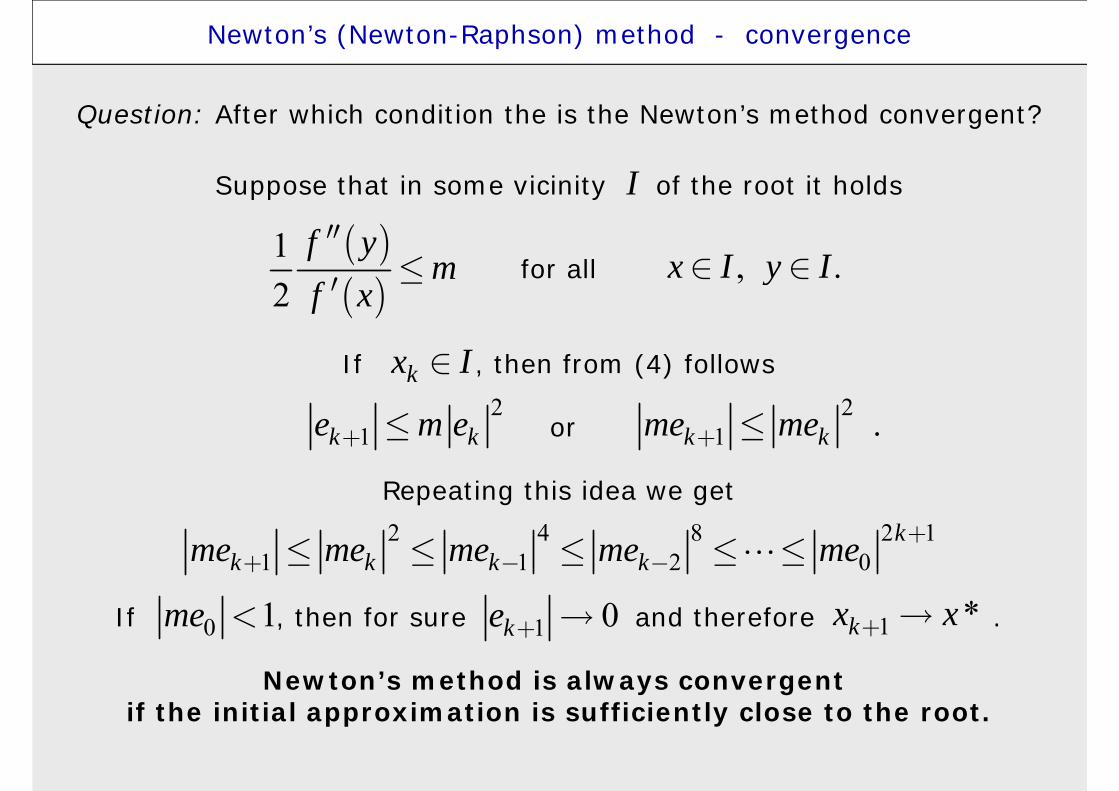
Newton’s (Newton-Raphson) method - convergence
Question: After which condition the is the Newton’s method convergent?
Suppose that in some vicinity I of the root it holds
for all
If , then from (4) follows
or
Repeating this idea we get
If , then for sure and therefore .
Newton’s method is always convergent if the initial approximation is sufficiently close to the root.
( )( )
12
f ym
f x¢¢
£¢
, .x I y IÎ Î
kx IÎ2
1k ke m e+ £ 21 .k kme me+ £
2 4 8 2 11 1 2 0
kk k k kme me me me me ++ - -£ £ £ £ £
0 1me < 1 0ke + 1 *kx x+
Combined method
Good initial approximation can be obtained by bisection method.
Combination of bisection and Newton’s method leads toa combined method,
which is always convergent.
e.g. procedure rtsafe from Numerical Recipes;Newton’s method is applied only in the vicinity of the root,
otherwise the bisection method is used.This assures the fast convergence.
0x

Lecture 2
CONTENTS
1. Introduction2. Root separation and estimation of initial approximation3. Bisection method4. Rate of convergence5. Regula falsi (false position) method6. Secant method7. Newton’s (Newton-Raphson) method8. Steffensen’s method9. Fixed-point iteration10. Aitken Extrapolation11. A few notes12. Literature
Steffensen’s method
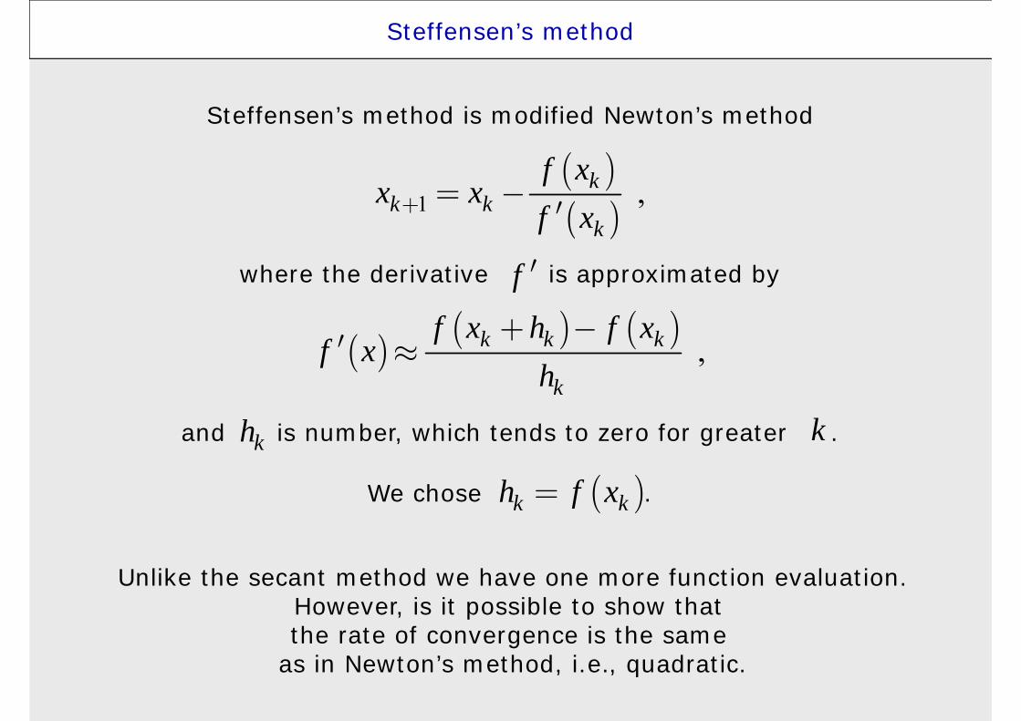
Steffensen’s method is modified Newton’s method
where the derivative is approximated by
and is number, which tends to zero for greater .
We chose .
Unlike the secant method we have one more function evaluation.However, is it possible to show thatthe rate of convergence is the same
as in Newton’s method, i.e., quadratic.
( )( )1 ,k
k kk
f xx x
f x+ = -¢
f ¢
( )( ) ( )
,k k k
k
f x h f xf x
h+ -
¢ »
kh k
( )k kh f x=
Lecture 2
CONTENTS
1. Introduction2. Root separation and estimation of initial approximation3. Bisection method4. Rate of convergence5. Regula falsi (false position) method6. Secant method7. Newton’s (Newton-Raphson) method8. Steffensen’s method9. Fixed-point iteration10. Aitken Extrapolation11. A few notes12. Literature
Functional analysis
Metric space
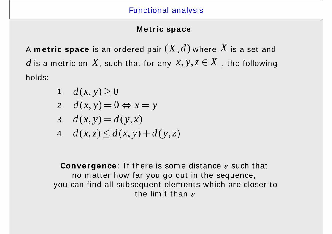
A metric space is an ordered pair where is a set and
is a metric on , such that for any , the following
holds:
1.
2.
3.
4.
( , )X d Xd X , ,x y z XÎ
( , ) 0d x y ³( , ) 0d x y x y= =( , ) ( , )d x y d y x=( , ) ( , ) ( , )d x z d x y d y z£ +
Convergence: If there is some distance such that no matter how far you go out in the sequence,
you can find all subsequent elements which are closer tothe limit than
Functional analysis
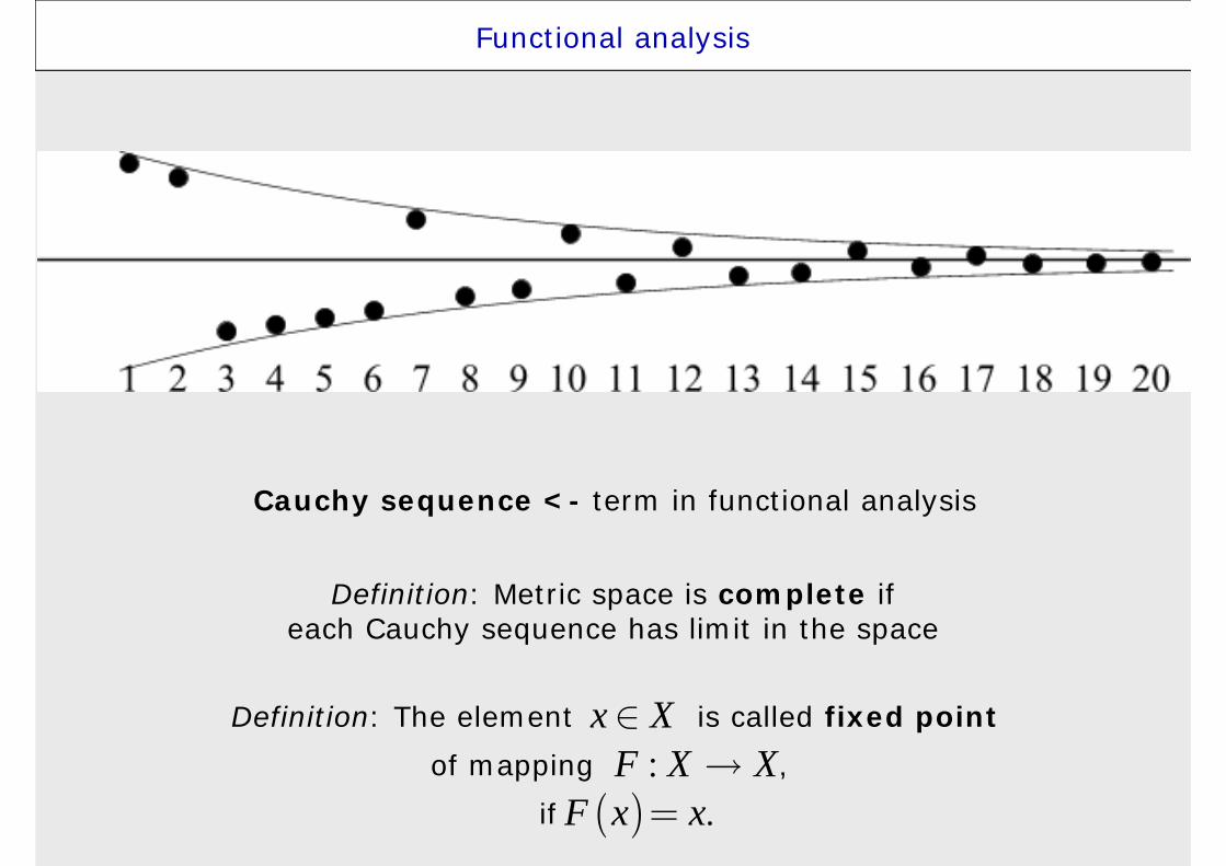
Cauchy sequence <- term in functional analysis
Definition: Metric space is complete ifeach Cauchy sequence has limit in the space
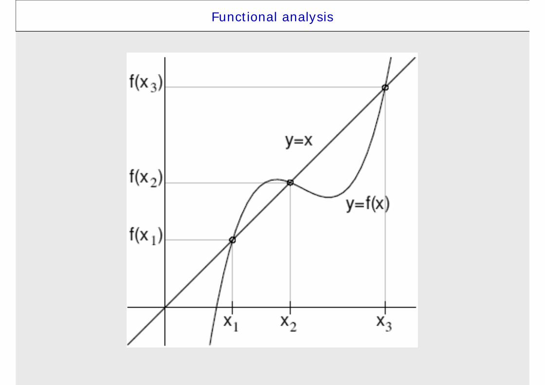
Definition: The element is called fixed pointof mapping ,
if:F X X
x XÎ
( ) .F x x=
Functional analysis
Functional analysis
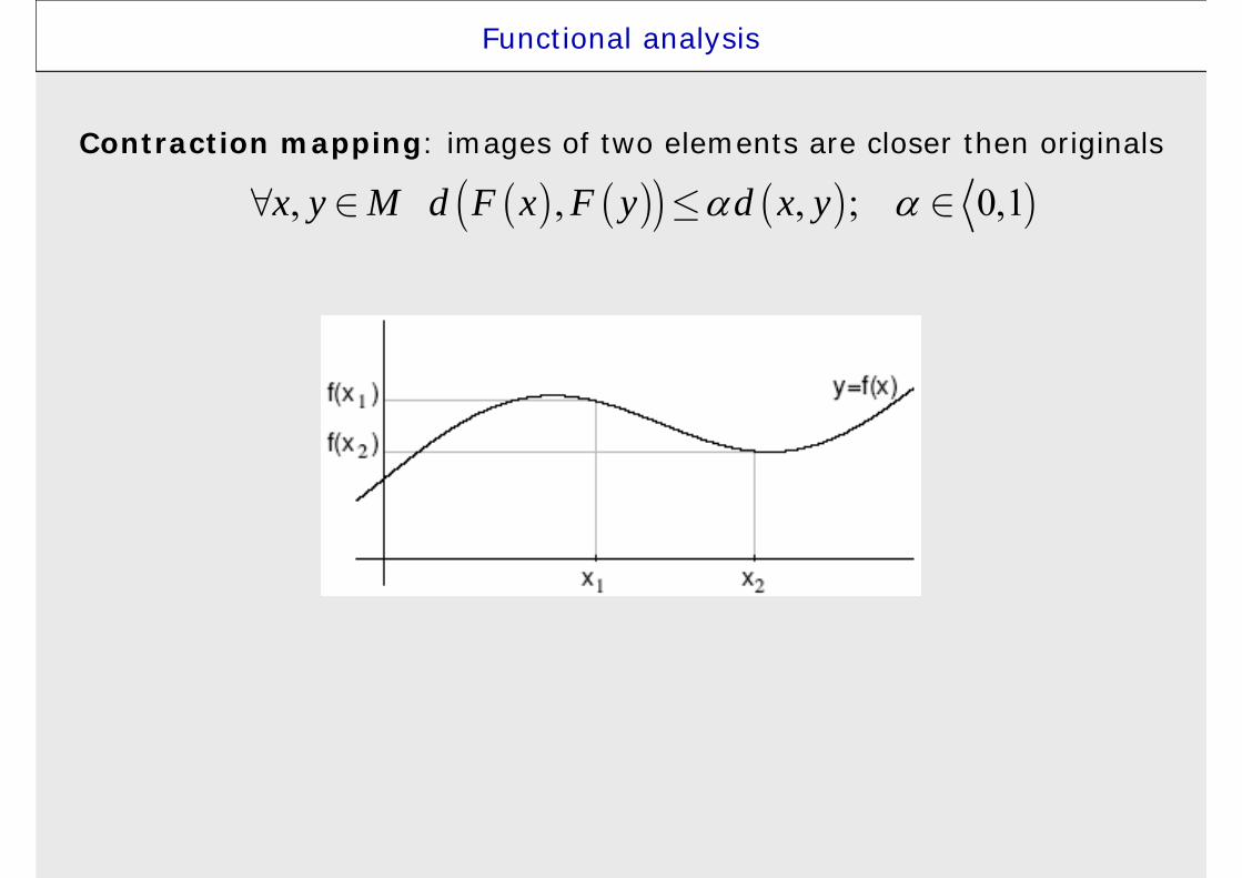
Contraction mapping: images of two elements are closer then originals
( ) ( )( ) ( ) ), , , ; 0,1x y M d F x F y d x y " Î £ Î
Functional analysis
Banach fixed-point theorem:
Let (X, d) be a non-empty complete metric space with a contraction
mapping . Then admits a unique fixed-point in . Furthermore, can be found as follows:
start with an arbitrary element in and definea sequence by , then .
:g X X
1( )n ng x x- =
g *x X*x
0x X{ }nx *nx x

Fixed-point iteration
What it is good for? Suppose we want to solve .
Let‘s rewrite the as , assuming .
We‘ll get fixed-point problem for .
while the solution of .
is root of .
Function g is called the iterative function.
We will chose the initial approximation andnext iterations will be .
( ) 0f x =
( )
( )( )
g x
f x x xh x
+ =
( )g x
( ) 0pf x =( )p pg x x=
( ) 0h x ¹( ) 0f x =
0x( )1 .k kx g x+ =
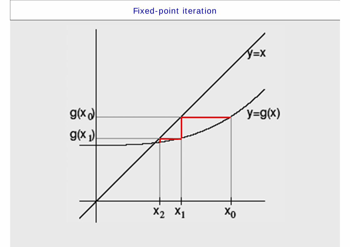
Fixed-point iteration
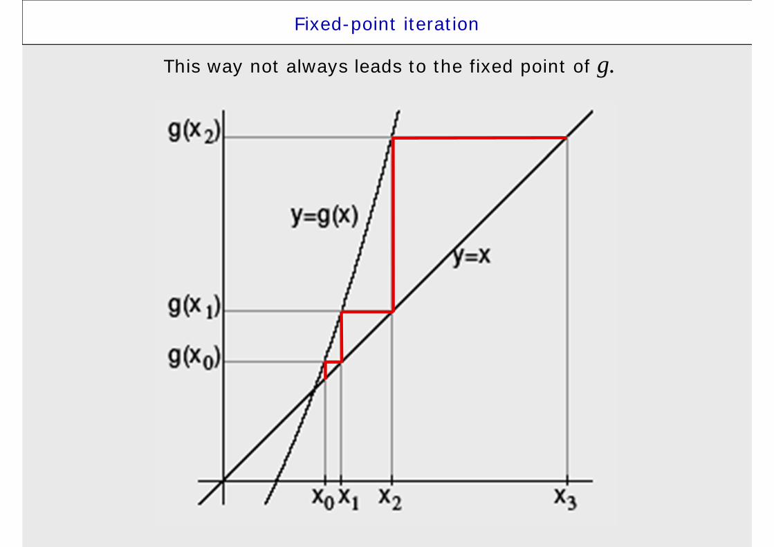
Fixed-point iteration
This way not always leads to the fixed point of g.
Fixed-point iteration
We said thatfixed-point iteration method converges
if the iterative function iscontraction mapping.
In case of function of one variable,contraction closely relates to
the rate of increase of function.
Fixed-point iteration
Theorem:Let function g maps an interval to itself
and g is derivative on this interval.If there exists number so that
then there exists fixed point of function g in interval andsequence of iterations
converges to the fixed point for any initial approximation .Next it holds
Then is it possible to show, that convergence is linear.
( )1k kx g x+ =
,a b
)0,1 Î
( ) , ,g x x a b¢ £ " Î
,a b*x
0 ,x a bÎ
1* .1k k kx x x x
-- £ --
Fixed-point iteration
The are many ways how to express from the .
One possibility is to divide the equation by its derivative f’,then multiply the equation by -1
and after all we add to both sides of equation .We get
( ) 0f x =x
( ) 0f x =
x
( )( )
.f x
x xf x
= -¢
Newton’s method is a special caseof fixed-point iteration method.
Lecture 2
CONTENTS
1. Introduction2. Root separation and estimation of initial approximation3. Bisection method4. Rate of convergence5. Regula falsi (false position) method6. Secant method7. Newton’s (Newton-Raphson) method8. Steffensen’s method9. Fixed-point iteration10. Aitken Extrapolation11. A few notes12. Literature
Aitken Extrapolation
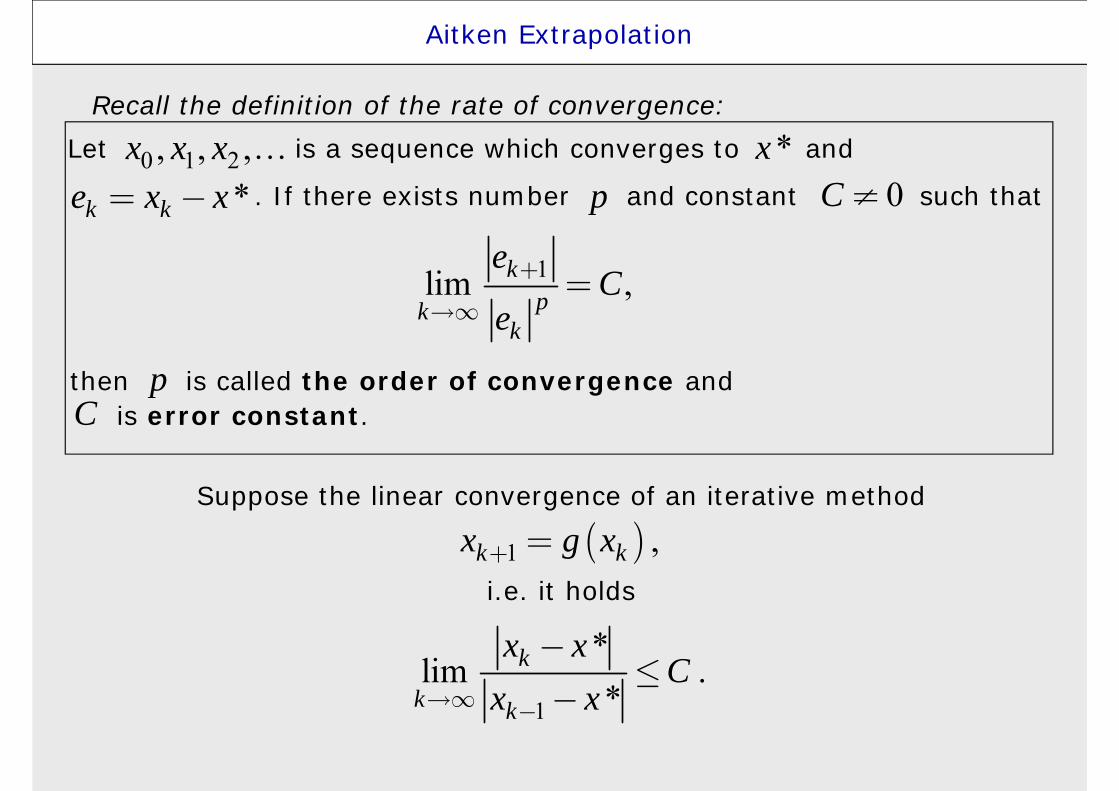
Suppose the linear convergence of an iterative method
i.e. it holds
1
*lim .
*k
k k
x xC
x x¥ -
-£
-
( )1 ,k kx g x+ =
then is called the order of convergence andis error constant.
pC
Recall the definition of the rate of convergence:Let is a sequence which converges to and
. If there exists number and constant such that0 1 2, , ,x x x *x
*k ke x x= - p 0C ¹
1lim ,kpk
k
eC
e+
¥=

Aitken Extrapolation
from which we could express the fixed point x*
( )1* * ,k kx x C x x-- » -
( )1 * * ,k kx x C x x+ - » -
( ) ( )( )
( )( )
1
12
1 1
2 2 21 1 1 1
21 1 1 1
21 1
1 1
* ** *
* * *
2 * * * *
* 2
*2
k k
k k
k k k
k k k k k k
k k k k k k
k k k
k k k
x x x xx x x x
x x x x x x
x x x x x x x x x x
x x x x x x x
x x xx
x x x
-
+
+ -
+ - + -
+ - + -
+ -
+ -
- -»
- -
- » - -
- + » - + +
- »- + +
-»
+ +
We can speed-up the convergence of fixed-point iteration as follows:Suppose that . Then it approximately holds1k

Aitken Extrapolation
from which we could express the fixed point x*
where .
This way we can define the new iterative formula
( )2211 1
11 1 1 1
* ,2 2
k kk k kk
k k k k k k
x xx x xx x
x x x x x x-- +
-+ - + -
--» = -
- + - +
( ) ( ) ( )( )1 1 1,k k k k kx g x x g x g g x- + -= = =
( )( )( )( ) ( )
2
1 .2
k kk k
k k k
g x xx x
g g x g x x+
-= -
- +
We obtained the Aitken-Steffensen iterative methodfor finding the fixed point of function .*x ( )g x
( )1* * ,k kx x C x x-- » -
( )1 * * ,k kx x C x x+ - » -
We can speed-up the convergence of fixed-point iteration as follows:Suppose that . Then it approximately holds1k

Aitken Extrapolation
If the initial approximation x0is close enough to fixed point x* and
if ,then Aitken-Steffensen method converges quadratically.
If , The convergence of this method is slow.
( )* 1g x¢ ¹
( )* 1g x¢ =
Lecture 2
CONTENTS
1. Introduction2. Root separation and estimation of initial approximation3. Bisection method4. Rate of convergence5. Regula falsi (false position) method6. Secant method7. Newton’s (Newton-Raphson) method8. Steffensen’s method9. Fixed-point iteration10. Aitken Extrapolation11. A few notes12. Literature
A few notes
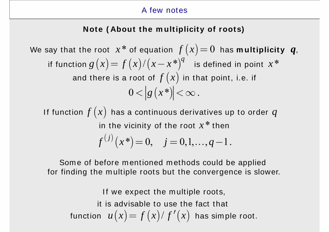
Note (About the multiplicity of roots)
We say that the root of equation has multiplicity q,
if function is defined in point .
and there is a root of in that point, i.e. if
If function has a continuous derivatives up to order .
in the vicinity of the root then
*x ( ) 0f x =( ) ( ) ( )/ * qg x f x x x= - *x
( )0 * .g x< <¥
( )f x q
( ) ( )* 0, 0,1, , 1.jf x j q= = -
*x
Some of before mentioned methods could be applied for finding the multiple roots but the convergence is slower.
If we expect the multiple roots,it is advisable to use the fact that
function has simple root.( ) ( ) ( )/u x f x f x¢=
( )f x
A few notes
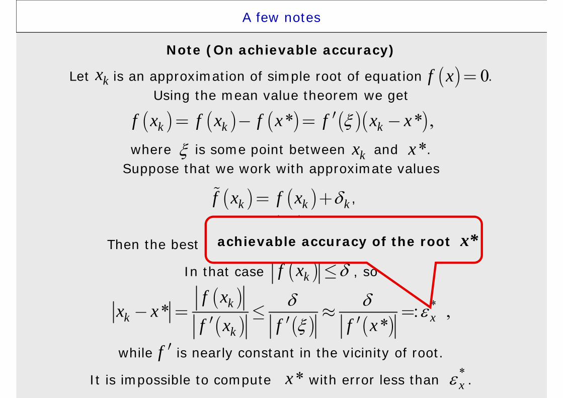
Note (On achievable accuracy)
Let is an approximation of simple root of equation .Using the mean value theorem we get
where is some point between and . Suppose that we work with approximate values
,
where .Then the best results we can achieve is .
In that case , so
while is nearly constant in the vicinity of root.
It is impossible to compute with error less than .
( ) 0f x =
( ) ( ) ( ) ( )( )* * ,k k kf x f x f x f x x¢= - = -
kx
*x kx
( ) ( )k k kf x f x = +
k £( ) 0kf x =
( )kf x £
( )( ) ( ) ( )
** : ,*
kk x
k
f xx x
f f xf x
- = £ » =¢ ¢¢
f ¢*x *
x
achievable accuracy of the root x*
A few notes
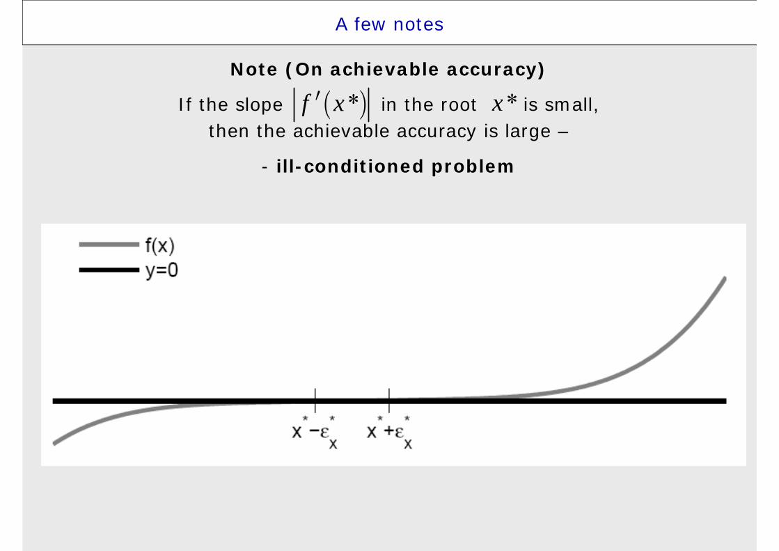
Note (On achievable accuracy)
If the slope in the root is small,then the achievable accuracy is large –
- ill-conditioned problem
( )*f x¢ *x
A few notes
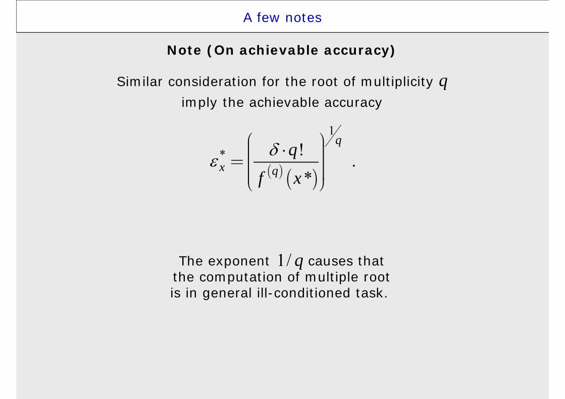
Note (On achievable accuracy)
Similar consideration for the root of multiplicity qimply the achievable accuracy
( ) ( )
1
* ! .*
q
x qq
f x
æ ö÷⋅ç ÷ç= ÷ç ÷ç ÷çè ø
The exponent causes thatthe computation of multiple rootis in general ill-conditioned task.
1/ q
Lecture 2
CONTENTS
1. Introduction2. Root separation and estimation of initial approximation3. Bisection method4. Rate of convergence5. Regula falsi (false position) method6. Secant method7. Newton’s (Newton-Raphson) method8. Steffensen’s method9. Fixed-point iteration10. Aitken Extrapolation11. A few notes12. Literature

Literature
• Press, W. H., Flannery, B. P., Teukolsky, S. A., Vetterling, W. T.:
Numerical Recipes in Fortran, The Art of Scientific Computing
Cambridge Universiy Press 1990
• Hämmerlin, G., Hoffmann, K. H.
Numerical Mathematics,
Springer-Verlag, Berlin 1991
• Quarteroni, A., Sacco, R., Saleri, F.
Numerical Mathematics
Springer, Berlin 2000