numerical differentiation and integration part...
TRANSCRIPT
Copyright © 2006 The McGraw-Hill Companies, Inc. Permission required for reproduction or display.
1
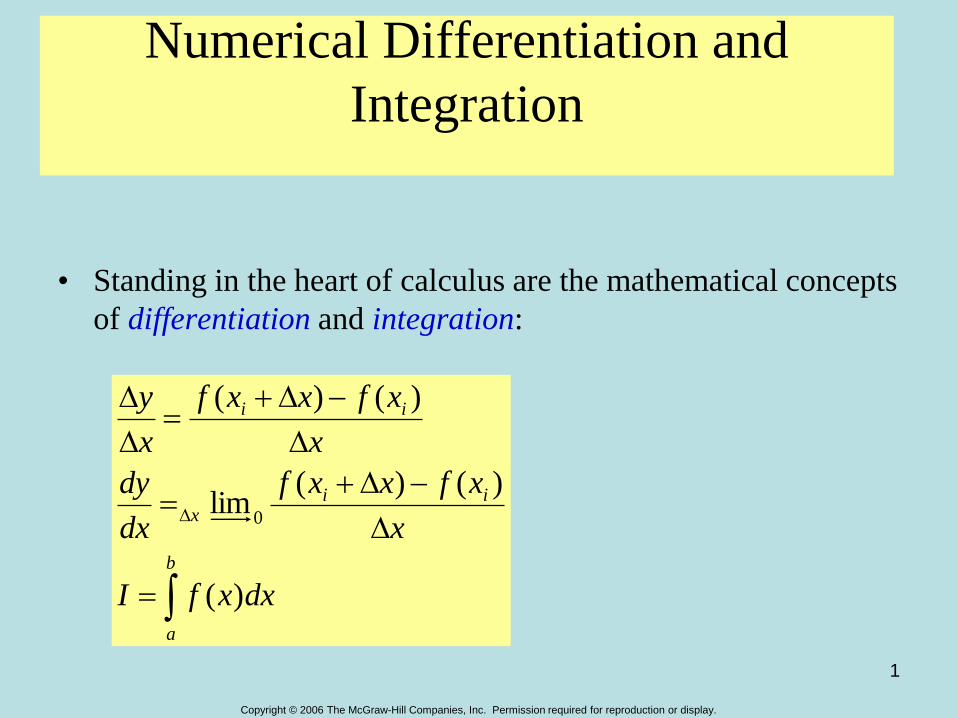
Numerical Differentiation and
Integration
• Standing in the heart of calculus are the mathematical concepts
of differentiation and integration:
b
a
iix
ii
dxxfI
x
xfxxf
dx
dy
x
xfxxf
x
y
)(
)()(lim
)()(
0

Copyright © 2006 The McGraw-Hill Companies, Inc. Permission required for reproduction or display.
by Lale Yurttas, Texas
A&M University
Chapter 21 2
Figure PT6.1

Copyright © 2006 The McGraw-Hill Companies, Inc. Permission required for reproduction or display.
by Lale Yurttas, Texas
A&M University
Chapter 21 3
Figure PT6.2

Copyright © 2006 The McGraw-Hill Companies, Inc. Permission required for reproduction or display.
by Lale Yurttas, Texas
A&M University
Chapter 21 4
Noncomputer Methods for
Differentiation and Integration
• The function to be differentiated or integrated will typically be in one of the following three forms:
– A simple continuous function such as polynomial, an exponential, or a trigonometric function.
– A complicated continuous function that is difficult or impossible to differentiate or integrate directly.
– A tabulated function where values of x and f(x) are given at a number of discrete points, as is often the case with experimental or field data.

Copyright © 2006 The McGraw-Hill Companies, Inc. Permission required for reproduction or display.
by Lale Yurttas, Texas
A&M University
Chapter 21 5
Figure PT6.4

Copyright © 2006 The McGraw-Hill Companies, Inc. Permission required for reproduction or display.
by Lale Yurttas, Texas
A&M University
Chapter 21 6
Figure PT6.7
Copyright © 2006 The McGraw-Hill Companies, Inc. Permission required for reproduction or display.
by Lale Yurttas, Texas
A&M University
Chapter 21 7
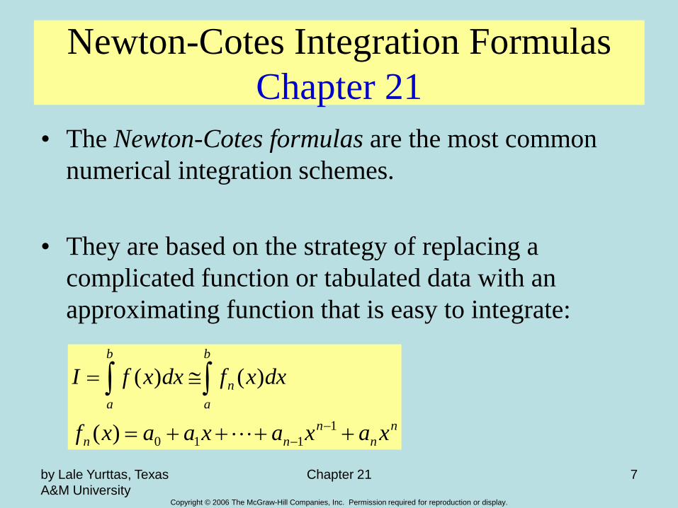
Newton-Cotes Integration Formulas
Chapter 21
• The Newton-Cotes formulas are the most common
numerical integration schemes.
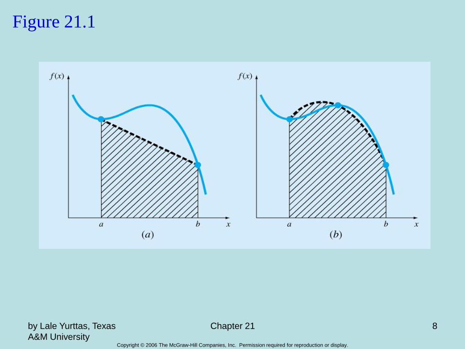
• They are based on the strategy of replacing a
complicated function or tabulated data with an
approximating function that is easy to integrate:
n
n
n
nn
b
a
n
b
a
xaxaxaaxf
dxxfdxxfI
1
110)(
)()(
Copyright © 2006 The McGraw-Hill Companies, Inc. Permission required for reproduction or display.
by Lale Yurttas, Texas
A&M University
Chapter 21 8
Figure 21.1

Copyright © 2006 The McGraw-Hill Companies, Inc. Permission required for reproduction or display.
by Lale Yurttas, Texas
A&M University
Chapter 21 9
Figure 21.2

Copyright © 2006 The McGraw-Hill Companies, Inc. Permission required for reproduction or display.
10
The Trapezoidal Rule
• The Trapezoidal rule is the first of the Newton-Cotes
closed integration formulas, corresponding to the
case where the polynomial is first order:
• The area under this first order polynomial is an
estimate of the integral of f(x) between the limits of a
and b:
b
a
b
a
dxxfdxxfI )()( 1
2
)()()(
bfafabI
Trapezoidal rule

Copyright © 2006 The McGraw-Hill Companies, Inc. Permission required for reproduction or display.
by Lale Yurttas, Texas
A&M University
Chapter 21 11
Figure 21.4
Copyright © 2006 The McGraw-Hill Companies, Inc. Permission required for reproduction or display.
by Lale Yurttas, Texas
A&M University
Chapter 21 12
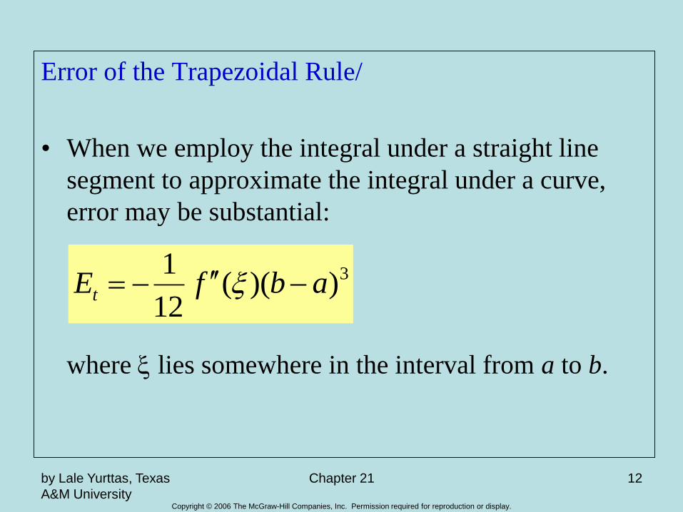
Error of the Trapezoidal Rule/
• When we employ the integral under a straight line
segment to approximate the integral under a curve,
error may be substantial:
where x lies somewhere in the interval from a to b.
3))((12
1abfEt x

Copyright © 2006 The McGraw-Hill Companies, Inc. Permission required for reproduction or display.
13
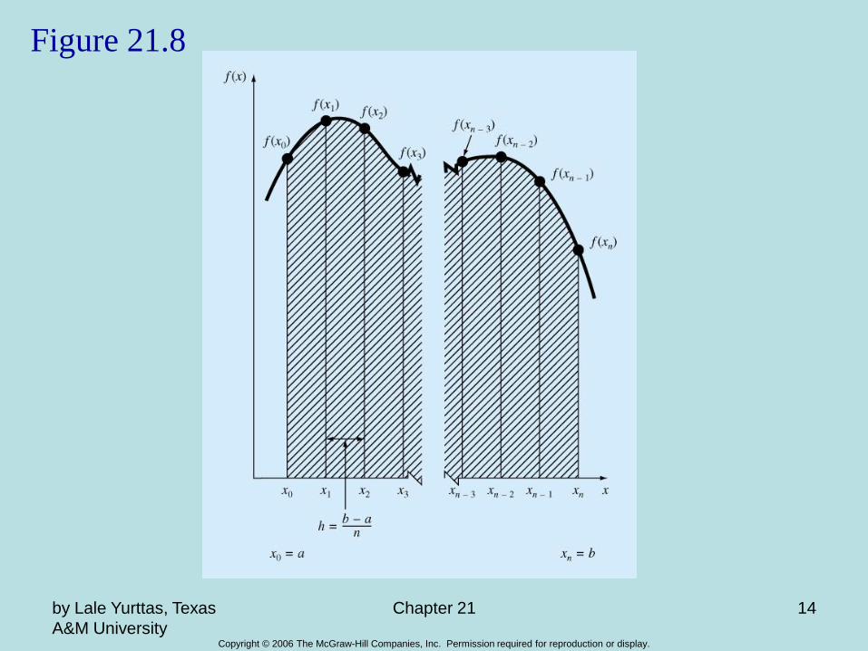
The Multiple Application Trapezoidal Rule/
• One way to improve the accuracy of the trapezoidal rule is to
divide the integration interval from a to b into a number of
segments and apply the method to each segment.
• The areas of individual segments can then be added to yield
the integral for the entire interval.
Substituting the trapezoidal rule for each integral yields:
n
n
x
x
x
x
x
x
n
dxxfdxxfdxxfI
xbxan
abh
1
2
1
1
0
)()()(
0
2
)()(
2
)()(
2
)()( 12110 nn xfxfh
xfxfh
xfxfhI
Copyright © 2006 The McGraw-Hill Companies, Inc. Permission required for reproduction or display.
by Lale Yurttas, Texas
A&M University
Chapter 21 14
Figure 21.8

Copyright © 2006 The McGraw-Hill Companies, Inc. Permission required for reproduction or display.
by Lale Yurttas, Texas
A&M University
Chapter 21 15
Simpson’s Rules
• More accurate estimate of an integral is obtained if a high-order polynomial is used to connect the points. The formulas that result from taking the integrals under such polynomials are called Simpson’s rules.
Simpson’s 1/3 Rule/
• Results when a second-order interpolating polynomial is used.

Copyright © 2006 The McGraw-Hill Companies, Inc. Permission required for reproduction or display.
by Lale Yurttas, Texas
A&M University
Chapter 21 16
Figure 21.10

Copyright © 2006 The McGraw-Hill Companies, Inc. Permission required for reproduction or display.
17
2
)()(4)(3
)())((
))(()(
))((
))(()(
))((
))((
)()(
210
2
1202
101
2101
200
2010
21
20
2
2
0
abhxfxfxf
hI
dxxfxxxx
xxxxxf
xxxx
xxxxxf
xxxx
xxxxI
xbxa
dxxfdxxfI
x
x
b
a
b
a
Simpson’s 1/3 Rule