numerical evidence of mode switching in the flow-induced...

Numerical evidence of mode switching inthe flow-induced oscillations by a cavity

Xavier Gloerfelt, Christophe Bogey and Christophe Bailly Laboratoire de M� canique des Fluides et dÕAcoustique

Ecole Centrale de Lyon & UMR CNRS 550969134 Ecully, France

e-mail: christophe .bailly@ec-lyon . fr

ABSTRACTA Direct Noise Computation (DNC) has been performed for a turbulent boundary layer past arectangular cavity, matching one configuration of Karamcheti1 experiments. An LES approachwith periodic boundary conditions in the spanwise direction is used to evaluate the solution at areasonable computational cost. The two components in the pressure spectra found experimentallyare well reproduced. The acoustic field appears to be dominated by the low-frequency componentwhereas the experimental visualization indicates a radiation at the higher frequency. The mechanismgiving rise to the lower frequency is investigated providing evidence on the possibility ofswitching between two cavity modes and that the strong coupling of the separated shear layerwith the recirculation flow within the cavity is likely to participate to the low-frequencymodulation. Moreover, an extrapolation method is proposed and applied to obtain the far-fieldfrom the near acoustic field.

1 INTRODUCTIONThe noise radiated by a flow past a cavity has been widely studied during the last fiftyyears because of its practical interest and because of the variety of theoretical questionsthat it raises. A complex feedback process sustains coherent oscillations in the shearlayer developing above the cavity. These oscillations often take the form of Kelvin-Helmholtz rolls, whose regular impingement on the front corner of the cavity produceshigh-intensity periodic acoustic waves. These pressure disturbances exert a feedbackinfluence on the selection of the shear layer instabilities. The pioneering work ofKaramcheti1 (1955) figures the externally radiated field through a Schlieren technique,and remains one of the few available measurements showing the structure of theacoustic field. This constitutes a great opportunity for the comparison with theComputational Aeroacoustics (CAA) tool. Cavity aeroacoustics is at the present timeone of the most popular test case for CAA because of its geometrical simplicity.The numerical investigation tool can help toward a better understanding of the noisegeneration mechanisms. The first 2-D CAA approaches2–5 using Direct Numerical

aeroacoustics volume 2 á number 2 á 2003 Ð pages 193 Ð 218 193

Simulation (DNS) of the full compressible Navier-Stokes equations have demonstratedthe feasibility of computing the frequency peaks and the structure of the radiated field.The strong upstream directivity agreed well with the visualisations of Karamcheti. Thenumerical constraints imposed by the DNS approach have limited these simulations2–5

to bidimensional, small-dimension, and high-speed configurations. The comparison withthe Karamcheti experiments using various length-to-depth ratios for rectangular cavitieswith a fixed 0.1 inch depth, spanning the transverse dimension of the wind tunnel, andwith freestream Mach numbers between 0.4 and 0.8, seemed therefore natural. Anotherinteresting issue in Karamcheti’s study is the different behaviour observed depending onwhether a laminar or a turbulent boundary layer interacts with the cavity, the aspect ratioand the stream velocity being kept constant. The frequency of the oscillations for aturbulent inflow is slightly lower than the one measured with a laminar inflow.Moreover, a low frequency appears in the spectra for a turbulent inflow. The origin ofthis low-frequency component, with roughly half the frequency of the fundamental,remains unexplained. Is it a subharmonic, a modulation of the impingement event, thepresence of a lower mode during the dominant mode, or an intermittent or deterministicswitching between two competitive cavity modes of oscillations?

The aim of this study is to use the numerical simulation, and its powerful analysiscapacity, to reproduce and characterize this low-frequency phenomenon. Intermittency ofthe shear-layer turbulence may lead to the multiple modes which apparently coexist. Thisconjecture6 has however few clear experimental illustrations. An alternance betweenmodes, called mode-switching is for instance observed in the experiments of Cattafestaet al.7 The fact that the vortices are rather clusters of small scales than single rolls in fullyturbulent shear layers, i.e. at high Reynolds numbers, may play a determinant role.

In an earlier work,8 a laminar configuration of Karamcheti’s experiments wassuccessfully reproduced for a cavity length-to-depth ratio , by using 2-D DNS.This reference solution has allowed the detailed comparison with three integralformulations to compute the acoustic far-field. However, the 2-D simulations arelimited to thick incoming boundary layer in order to avoid a bifurcation toward a so-called wake mode, where the dynamics of the shear layer is overwhelmed by therecirculating flow inside the cavity. This numerical artefact arises from the non-mixingof contrarotative vortices in a 2-D plane. A 3-D approach is required to reproduce thedynamics of the recirculation. Moreover, the simulation of a realistic turbulentboundary layer is necessarily three-dimensional. A DNS solving all the scales (down tothe Kolmogorov scale) becomes impractical in 3-D, and must be replaced by a methodusing turbulent modellings. The first one is Large Eddy Simulation (LES) where onlythe structures discretised by the meshgrid are computed, using the fact that the cavityflow is dominated by the interactions of coherent structures with the downstreamcorner.9,10 Larchevêque et al.9 performed LES of the 3-D flow over a cavity at a Mach number of 0.8, and a Reynolds number . Their resultscompare remarkably well with the corresponding experimental measurements byForestier et al.11 For high-Reynolds number flows, Shieh and Morris12 proposed theuse of a hybrid RANS/LES approach based on the Detached Eddy Simulation(DES) concept. This method aims at exploiting the best features of both approaches by

Re L = . ´8 6 105L D/ = .0 42

L D/ = 2

194 Numerical evidence of mode switching in the flow-induced oscillations by a cavity

solving RANS in the turbulent boundary layer and a one-equation LES in the separatedshear layer.

In the present study, a 3-D LES is performed for the moderate Reynolds numberconsidered in order to describe the behaviour of the small scales and the intermittencyof the turbulence. The effects of the unresolved subgrid scales are modelled via theSmagorinsky eddy viscosity with a self-adaptive Van Driest damping function near thesolid boundaries. The influence of this model and of the choice of the Smagorinskyconstant are discussed in the case of the development of a turbulent boundary layer. Theefficiency of the model in the separated shear layer above the cavity is only brieflyaddressed, since no aerodynamic measurement is available for this configuration. Thestandard Smagorinsky model is seen to be often too dissipative in high Reynoldsnumber flows.13 It can be inferred that the eddy viscosity may have a non-negligibleeffect on the shear layer dynamics, and that a less dissipative model would be helpfulto preserve high Reynolds number features.

Another modelling issue concerns the prescription of a realistic turbulent boundarylayer ahead of the cavity. Perturbations are superimposed on an initial turbulent profilein the inlet plane in order to bypass transition, and accelerate the eruption of trueturbulence ahead of the cavity. A turbulent boundary layer with zero pressure gradientis simulated to check the rapid spatial development of realistic turbulence.

Since most of the previous turbulent boundary layer simulations used periodic boundaryconditions in the spanwise direction, and also to account for the very large length-to-widthratio in the Karamcheti experiment, the lateral boundary conditions are assumed periodicfor the flow. Only a slice of the physical domain is computed, reducing the numericalcost. This assumption is physically justified since the main features of cavity flows arefound to be bidimensional for length-to-width ratios , as shown by Ahuja andMendoza.14 The 3-D character of the simulation is necessary to describe the turbulentmixing but a high degree of coherence is observed in the spanwise direction.

Despite the grid limitation, a large range of length and time scales are still involved,from the small structures of the turbulent boundary layer to the long wavelengths of theacoustic waves. To cope with this, the computational domain is often truncated in anacoustic region not too far beyond the unsteady flow. A simple method must then beapplied to extend the acoustic near-field from the cavity Direct Noise Computation(DNC) to the far-field in order to ensure that cancellations and superpositions that mayoccur in the acoustic region do not change the structure of the far-field. Severalnumerical methods for extending the sound field have been proposed. One approach isto use wave equation solutions formulated as a surface integral such as the Kirchhoff orFfowcs Williams and Hawkings Wave Extrapolation Methods which have been appliedto jet15,16 or cavity simulations.8 The far-field solution is then expressed as a singleintegral, reducing the computational requirements. This is particularly convenient whenonly a directivity using few sensors is needed. Nevertheless, the integral formulationsrequire data for all the retarded times from sound emission until reception. When thesource region is very extended, the temporal storage needed to evaluate the integralsolution is large. These methods become hardly practical due to computer memorylimitations. Moreover the integral methods assume an acoustic medium with constant

L W/ < 1

aeroacoustics volume 2 á number 2 á 2003 195

properties, so that they cannot deal with nonlinear propagation. Another solution,proposed by Freund et al.17 or Shih et al.,18 consists in matching the Navier-Stokessolver to a far-field region where a wave equation or a similar set of acoustic equationsare solved. The implementation is simpler since the data are now only neededsequentially. The matching should allow for two-way communication between thedomains. In the present work, to avoid the matching region necessary for transferringinformations from the acoustic grid to the DNC grid, a slightly different method isproposed. The DNC is made independent of the extrapolation method by using twogrids with different boundary conditions. The acoustic solver is thus easier to couplewith the DNC since no transfer from the coarse grid to the fine grid is needed, allowingthe use of a much larger meshsize and time step in the acoustic calculation.

The paper is organised as follows. In the first part, the numerical methods used for the3-D Direct Noise Computation of cavity aeroacoustics are described. The second partpresents the results of the simulation for the , turbulent configurationof Karamcheti’s experiments.1 The switching between two cavity modes is demonstrated.

2 NUMERICAL METHODS FOR THE DIRECT NOISECOMPUTATION

2.1 Governing equations3-D filtered Navier-Stokes equations for compressible fluidsA schematic view of the flow domain is shown in figure 1. The origin of the coordinatesystem is located at the middle of the upstream corner. For the Direct NoiseComputation, the full three-dimensional compressible Navier-Stokes equations aresolved to simulate both the flow and the acoustic perturbations. They are expressed ina conservative form in the Cartesian coordinate system of figure 1. In Large EddySimulation, only the scales larger than the grid size are computed explicitely, and thesubgrid scales are modelled. The governing equations are obtained after spatialfiltering, denoted by a bar. The velocity components are decomposed into a resolvedpart, , using Favre averaging, and an unresolved part, . The resultingsystem solved in the present study is:

(1)

with:

U

E

F

G

e

e

e

= , , , ,

= , + , , , +

= , , + , , +

( ˜ ˜ ˜ ˜)

( ˜ ˜ ˜ ˜ ˜ ˜ ( ˜ ) ˜ )

( ˜ ˜ ˜ ˜ ˜ ˜ ( ˜ ) ˜ )

r r r r r

r r r r r

r r r r r

u u u e

u p u u u u u e p u

u u u p u u u e p u

t

t

t

1 2 3

12

1 1 2 1 3 1

2 2 1 22

2 3 2

== , , , + , +

= , + , + , + , + - -

= , + , + ,

( ˜ ˜ ˜ ˜ ˜ ˜ ( ˜ ) ˜ )

( ˜ ˜ ˜ ˜ ( ˜ ) ˜ )

( ˜ ˜ ˜

r r r r r

t t t t

t t t

u u u u u p u e p u

u q c

t

i i i vt

3 3 1 3 22

3 3

11 11 12 12 13 13 1 1 1 1

21 21 22 22

0

0

E

F

v

v

T T T T Q

T T 2323 23 2 2 2 2

31 31 32 32 33 33 3 3 3 30

+ , + - -

= , + , + , + , + - -

T T Q

T T T T Q

˜ ( ˜ ) ˜ )

( ˜ ˜ ˜ ˜ ( ˜ ) ˜ )

u q c

u q c

i i i vt

i i i vt

t

t t t tGv

¶¶

+¶¶

+¶¶

+¶¶

-¶¶

-¶¶

-¶¶

=U E F G E F Ge e e v v v

t x x x x x x1 2 3 1 2 3

0

¢¢uiu ui i= /r r

M = .0 8L D/ = 3


where is the specific heat at constant volume. The quantities , , are the resolveddensity, pressure, and velocity components. For a perfect gas, the total energy per massunit is defined as:

where is the temperature, the gas constant, and the ratio of specific heats.The viscous stress tensor is modelled as a Newtonian fluid , where isthe dynamic molecular viscosity, and the deviatoric part of the resolved deformationstress tensor:

The heat flux component models thermal conduction in the flow with Fourier’s law, where is the Prandtl number, and the specific heat at

constant pressure.

Subgrid-scale modellingThe effects of the subgrid scales are present in system (1) through the subgrid scalestress tensor and the subgrid scale heat flux , respectively:

A simple closure model consists in reproducing the dissipative effets of the unresolvedscales by implementing a turbulent viscosity , a subgrid scale energy , and aturbulent Prandtl number . The subgrid scale tensor and heat flux can then bemodelled by:

T Qij t ij sgs ij it

t i

S kT

x= - , = - ¶

¶2

23

m r d ms

˜˜

and

s t

ksgsmt

T Qij i j i j i i iu u u u u T u T= - - , = -r r( ˜ ˜ ˜ ˜ ) ( ˜ ˜ ˜ )

QiT ij

cps˜ ( )( ˜ )q c T xi P i= - / ¶ /¶m sqi

˜ ˜ ˜ ˜S

u

x

u

x

u

xiji

j

j

iij

k

k

=¶¶

+¶¶

-¶¶

æ

èç

ö

ø÷

1

2

2

3d

Sij

m˜ ˜t mij ijS= 2t ij

grT

˜ [( ) ] ( ˜ ˜ ˜ ) ˜e p u u u p r T= / - + + + / , = ,g r r1 221

22

23 and

e

uiprcv


0

x2

x3

x1W

D

L

Figure 1. Sketch of the flow domain and coordinate system.

We choose the Smagorinsky eddy-viscosity model, where , is

the Smagorinsky constant, and the characteristic length scale.Values of approximately are typically used for wall-bounded flow.19 Thesensitivity to this choice is discussed in paragraph 2.3. The subgrid scale energy isnot directly available, but, following Erlebacher et al.,20 it is modelled as

, where . Lastly, the turbulent Prandtl number is takenconstant, . In the following, the tilde notation is omitted since only resolvedquantities are studied.

Wall model One of the major drawback of the previous modelling is that the Smagorinsky model isnot able to describe the scale reduction that occurs near the solid walls. A solutionconsists in superimposing an empirical wall law for near the solid boundaries. Moinet Kim21 and several authors propose to weight the characteristic length scale by theexponential van Driest damping function:

where and is the normal wall coordinate. The friction speedis determined by solving the logarithmic law for every point on the walls:

with designing the mean longitudinal velocity and the kinematic viscosity.

2.2 Algorithm and boundary conditionsAlgorithmThe convective terms of (1) are integrated in time using an explicit low-storage six-stepRunge-Kutta scheme optimised in the wave number space. Because of their slower timeevolution, the viscous terms are only integrated in the last substep. The gradients aresolved on a rectangular slowly nonuniform grid by using optimised finite-differencesfor an eleven-point stencil for the convective fluxes, and standard 4th order finitedifferences for the viscous and heat fluxes. As part of the algorithm, a selective filteringbuilt up on an eleven-point stencil is incorporated in each direction to eliminate grid-to-grid unresolved oscillations. The coefficients of the Runge-Kutta algorithm, of thefinite differences and of the filtering are given in Bogey and Bailly.22

Solid wallsOn all solid boundaries, the no-slip conditions are imposed, with

, where is the direction normal to the solid surface. The finite-differencen¶ / ¶ =p n 0u u u1 2 3 0= = =

nu1

u x x

u x

x u x1 1 2

1

2 15 75 5 24 0( )

( )log

( ), - . æè

öø + . =

t

t

n

utx x u2 2+ = /t nA+ = 25

D = -æèç

öø÷

ìíï

îï

üýï

þïD

+

+c cx

A’ exp1 2

D c

mt

s t - .0 1CI - .0 1k C S Ssgs I c ij ij= D2 2r ˜ ˜

ksgs

CS = .0 1D = D D D /

c x x x( )1 2 31 3

CSm rt S c ij ijC S S= D( ) ˜ ˜2 2


stencil for the convective terms is progressively reduced down to the fourth order.The viscous stress terms are evaluated from the interior points by using fourth orderbackward differences. The wall temperature is calculated with the adiabatic condition.For the sharp corners formed by the intersection of planar cavity surfaces, the variablesare determined by using the interior scheme, thereby avoiding any ambiguity regardingthe normal direction.

Radiation conditionsAt the upstream and upper boundaries of the computational domain, the radiationboundary conditions of Tam and Dong,23 using a far-field solution of the sound waves,are applied. The origin of the acoustic waves is located at the downstream corner, ( , , ). It must be noted that the exact location of the sound sourceis not very important if the boundaries are sufficiently far from the sources.24 However,the choice of a vertical location at is well-suited to the implementation of theinflow and outflow boundary conditions near the walls. At the outlet, the outflowboundary conditions of Tam and Dong, where the radiation solution is modified toallow the exit of vortical and entropic disturbances, is combined with a sponge zonedissipating vortical structures. This sponge zone uses grid stretching and aprogressively applied Laplacian filter.

Lateral boundariesWhen the cavity span is smaller than the width of the computional domain, thesidewalls can be modelled by using the wall condition. But to account in thepresent simulation for the very large length-to-width ratio used in the Karamchetiexperiment , periodic boundary condition are applied for the lateralboundaries.

2.3 Generation of a spatial turbulent boundary layerMost of the earlier computations of turbulent boundary layers has been limited totemporal simulations based on the quasi-periodicity of the flow in the streamwisedirection. For spatially evolving boundary layers, needed in the present work, thecomputational region must include both the transition region and the turbulent region,and requires far greater computational resources. The three-dimensional simulation ofthe natural transition of a flat-plate boundary layer has only become possible recently.25,26

A high level of accuracy is required in order to reproduce the development of Tollmien-Schlichtling waves and their breakup through secondary and tertiary instabilities.It is obviously too expensive for the present investigation since the attention is primarilyfocused on the interactions with the cavity. A bypass transition appears more appropriate.Voke & Yang27 show for instance that since the transition is thus early and short, thedetailed computation of the instabilities is not crucial. In the present work, an initialturbulent mean profile is used to accelerate the eruption of developed turbulence aheadof the cavity.

To create unsteady, stochastic inlet conditions, we use a synthetic flowfield, basedon Random Fourier Modes (RFM).28 The turbulent inlet field is generated as the sum

( / . )L W = 0 03

x2 0=

x3 0=x2 0=x L1 =


of independent RFM, with amplitudes determined from the turbulent kineticenergy spectrum. The fluctuating velocity field is then expressed as a Fourier series:

where , , are random variables with given probability density functions. Anunfrozen turbulent field is obtained by incorporating the convection velocity and thepulsation , accounting for the temporal evolution of the perturbations. In the presentturbulent simulation, and is deduced from the Heisenberg time,

, where is the fluctuating velocity and the wave number.The turbulent boundary layer with zero pressure gradient is first chosen as

a fundamental testcase to study the development of a realistic turbulent inflow. Basedon DNS and LES of the literature, the size of the computational domain is takenequal to in the streamwise direction and in the vertical direction,being the displacement thickness given below. The spanwise extent is , withperiodic boundary conditions. The Cartesian meshgrid is points, with constant spacings in the and directions, and 3% stretching in the

-direction. The grid spacings in wall units, nondimensionalised by, are , , and , where m/s is obtained from

the logarithmic law. The Mach number of the flow is 0.5. The simulation is initialisedwith the mean profile from Spalart’s29 temporal boundary layer simulation at

, extrapolated into the entire computational domain. The stochasticturbulent field, generated by the method described above, is weighted by the verticalprofiles of velocities from Spalart’s29 temporal DNS, and is superimposed on themean profile. Tam and Dong’s radiation boundary conditions are applied on the freeboundaries. 30000 temporal iterations are performed with s, and is taken equal to 0.1.

Figure 2 shows contours of the calculated vorticity. The onset of realistic turbulenceis seen to occur roughly after in the streamwise direction. The flow structurehas then similarities with the results of Spalart or with experimental smoke pictures.30

In the region where the boundary layer is estimated to be fully established, at

, the boundary layer thickness is m, the displacement thickness is m, and the momentum thickness m,giving a shape factor . The Reynolds number based on the momentumthickness is . Spalart29 gives for . To demonstratethat a log layer exists within the turbulent boundary layer, the longitudinal mean velocity

is plotted on semilog coordinates in figure 3(a). A well-defined log region is visible even if the viscous sublayer is not resolved by the meshgrid used. Moreover,to ascertain that a inertial subrange exists, spectra of the kinetic energy are evaluated ata distance from the wall, for , and averaged over 7 locations in thehomogeneous spanwise direction. The spectra used 2000 samples of the velocityfluctuations recorded every 10 temporal iterations. The energy spectrumof figure 3(b) shows the typical law in the inertial subrange.- /5 3

x1 62= *d0 5. d

u u u1 1+ = / t

Redq= 1410H = .1 42Redq

= 1410H = / = .*d dq 1 42

dq = . ´ -1 23 10 4d * -= . ´1 75 10 4d = . ´ -1 26 10 3x1 62= *d

50d *

CSD - ´ -t ˜ 2 10 8

rms

Redq= 1410

1 2u x( )

ut = .7 8D =+x3 20D =+xmin2 5D =+x1 50n t/u

x2

x3x1

201 91 121´ ´28d *

d *25d *114d *

knrms¢uw pn nu k= ¢2wnN = 200

wn

uankny n

¢ , = . - + +=åu x k x u a( ) ˆ cos( ( ) )t u t tn

N

n n n n n

1

w y

nuN



Figure 2. Turbulent boundary layer testcase. Vorticity isocontours: topview ofat , sideview of at , and crossview of at

. (——): positive contours ; (– – –) : negativecontours .- - -[ ] ´10 1 0 1 105; ; .

0 1 1 10 105. ; ;[ ] ´x1 86= d*

w23x3 0=w12x2 0 6= . *dw13

Figure 3. Turbulent boundary layer testcase. Mean profile of (a): ( ), presentLES; (++), Spalart’s DNS29; (– – –), linear law; (– . – . ), logarithmic law;(——), analytical Van Driest profile. Energy spectrum of vertical velocityfluctuations (b) in the boundary layer at a distance of from the wall.0 5. d

o ou u1 / t

An important question regards the influence of the choice of the Smagorinskyconstant on the flow dynamics. Figure 4 shows the vertical variation of the turbulenceintensities obtained for three values of : the standard value of 0.18 for isotropicturbulence, the value of 0.1 commonly used for wall-bounded flow, and a lower valueof 0.02. Comparison of these distributions with those of Spalart’s simulation29 indicates

CS

fairly good agreement for all cases. The only slight differences are seen near the solidwalls with larger gradients for smaller values of the constant. The weak sensitivity tothe value of indicates that the turbulent boundary layer is well resolved by the present numerical method. The use of high-order schemes, such as those optimised byBogey and Bailly,22 is seen to be crucial with the aim of computing accurately the resolvedscales by LES because of their low intrinsic numerical dissipation. It was particularlyshown that since the filtering affects only the short waves discretised by less than four gridpoints, the features of the resolved scales are independent on this artificial energy-dissipating process.31

CS


0 0.2 0.4 0.6 0.8 1 1.20

0.5

1

1.5

2

2.5

x2 / d

u i+

x2 / d

u i+

0 0.2 0.4 0.6 0.8 1 1.20

0.5

1

1.5

2

2.5

x2 / d

u i+

0 0.2 0.4 0.6 0.8 1 1.20

0.5

1

1.5

2

2.5

(a) (b)

(c)

Figure 4. Turbulent boundary layer testcase. Turbulent intensities for the spatialLES (symbols) and the temporal DNS of Spalart29 (lines): ( ,——),

; ( , – . – . ), ; (**, – – –) . Three values ofthe Smagorinsky constant are tested: (a), (b), and

(c).Cs = 0 02.Cs = 0 1.Cs = 0 18.

u urms3 / tu urms2 / t+ +u urms1 / t

o o

The main features of the spatial development of a turbulent boundary are thussatisfactorily reproduced by using RFM to bypass the transition. The multiplication of thestochastic velocity by given vertical profiles of velocities ensures a shorter transitionalregion but has two drawbacks. First, the incompressibility condition is no longer ensuredand the excitation becomes noisy, but this spurious radiation is however sufficiently weakcompared to cavity noise. Second, it cannot provide the phase relationship betweenindividual Fourier modes, and turbulence decays downstream of the inlet plane until thenear wall cycle of turbulence production has been established.

2.4 Resolution of the cavity configurationThe simulation matches one configuration of Karamcheti’s experiments,1 for a length-to-depth ratio , and a Mach number M = 0.8, with mm as in theexperiment. The computational box extends over horizontally and 6.5D vertically.The slice simulated has a spanwise width of . The meshing is slowly nonuniformand Cartesian, with grid points inside the cavity andoutside, clustered near the walls. A resolution , , and isreached. The time step is s, to satisfy the CFL stability criterion withCFL = 0.66. The computation lasts 43 hours on a Nec SX-5, for 4.9 million grid-pointsand 70000 iterations.

The computation is initiated by extrapolating the mean inflow velocity profile intothe entire computational domain. The freestream air temperature is K, and thestatic pressure is taken as 1 atm.

2.5 Method for extending near-field to far-fieldBeyond an extrapolation surface, specified by the DNC near-field, the extrapolationmethod solves the isentropic Linearised Euler Equations (LEE),

with and , the freestream values from the cavity DNC. Owing to thehigh subsonic Mach number, M = 0.8, and the high-level pressure waves generated bythe interaction with the downstream corner of the cavity, the propagation is nonlinear.To cope with this, the sound speed can vary to include a part of the eventual nonlinear effects on wave propagation. The first order modification from the weak shockwave theory32 is implemented:

This simple modification allows the inclusion of the main part of the nonlinear effects(including the term) with almost no additional cost. A better description of the( )¢.Ñ ¢u u

c cp

p0 11

2= + + ¢æ

èçöø÷¥

¥

gg

c0

r r0 = ¥U U0 = ¥

¶ ¢¶

+ ¶ ¢¶

+ ¶ ¢¶

= = , ,

¶ ¢¶

+¶ ¢¶

+ ¶ ¢¶

=

ì

íïï

îïï

i i

i

j

j

ut

U ux

p

xi

p

tc

ux

Up

x

01 0

0 02

01

10 1 2 3

0

r

r

{ }

p¥

T¥ = 320

D = . ´ -t 1 95 10 8D -+x3 34˜D -+x

min2 9˜D -+xmin1 28˜

271 140 101´ ´101 101 101´ ´1 6. D

13DD = .2 54L D/ = 3

rms


nonlinear steepening would only be possible through the use of the complete energyequation. The new set of simplified equations resolved in the acoustic part is nowweakly nonlinear, and is referred to as Weakly Non Linear Euler Equations (WNLEE)in the following.

A view of the two meshgrids used for the DNC and for the WNLEE calculation ispresented in figure 5. It shows the DNC region on the bottom where the full Navier-Stokes equations are solved on a non regular Cartesian grid refined near the horizontaland vertical walls of the cavity, and the acoustic region on the top where WNLEE aresolved on a regular Cartesian grid. The extrapolation surface is located at .In order to validate the results obtained with the extrapolation method, the regionbetween and is resolved by both methods. In the DNC,radiation conditions are used for the three free-field sideview boundaries. Periodicconditions are applied for the two spanwise boundaries. In the WNLEE simulation, thesame boundary conditions are used to allow a comparison with the DNC. The regularCartesian grid in figure 5 represents the acoustic region with points and

. It extends from to . Its streamwiselength is slightly larger than that of the DNC, from to . Thespanwise dimension is the same as that chosen for the DNC. For comparison, the DNC

x D1 8/ =x D1 6/ = -x D2 13/ =x D2 2/ =D = D = D = .x x x D1 2 3 0 078

181 151 21´ ´

x D2 5 5/ = .x D2 2/ =

x D2 2/ =


Figure 5. Superimposition of the meshgrids used for the DNC (bottom) and for theWNLEE calculation (top). The grids are shown every other four points(sideview on the left and crossview on the right).

region uses grid points above the cavity, and covers onlyvertically. The refinements near the two vertical walls of the cavity, and all along thespanwise direction, needed to describe accurately the flow, induces an additionaldiscretisation cost in the acoustic part due to the Cartesian representation. A factorof 7 can be saved with the meshgrid of the extrapolation method. In the verticaldirection, the meshsize used for the WNLEE is the same as the meshsize near theextrapolation surface in the DNC. The frequency cut-off of the acoustic simulation istherefore identical to that of the DNC based on near , thus smaller thanthat at the limit of the DNC domain. Moreover, the use of a regular grid minimizes thedissipation and the dispersion of the numerical schemes, which have been optimised fora constant meshsize.22 The time step imposed by the CFL criterion is proportional to thesmaller gridsize, near the walls in the DNC and for theregular mesh. We see roughly a factor 20 decrease in computational cost. In addition,comparing the 7 spatial derivatives for the WNLEE to the 39 derivatives necessaryfor the Navier-Stokes solver, the computing expense is further reduced by a factorof 5.5. The WNLEE has also fewer field variables and thus smaller memoryrequirements. Then the global reduction of computer time is more than 700 for theextrapolation method. The WNLEE are solved with the same eleven-point stencildifferencing, six substep Runge-Kutta technique, and eleven-point stencil filtering asthe Navier-Stokes DNC region. The free-field boundary conditions use Tam and Dong’sformulation.

3 MODE SWITCHING BETWEEN TWO CAVITY MODES3.1 Features of the unsteady flowThe spectrum of the LES pressure fluctuations near the impingement corner is shownin figure 6(a), and exhibits two well-defined peaks. The higher frequency correspondsto a Strouhal number and the lower frequency occurs at

with a level 5 dB greater. The values measured by Karamcheti1 for thisconfiguration and are in good agreement as seen in thecomparison of figure 6(b). Karamcheti observed a single peak when the incomingboundary layer was laminar with a Strouhal number , slightly higher than

. The appearance of two components, for a turbulent boundary layer, was noted.The time trace of the pressure fluctuations in figure 7 is analysed to identify the portionsof the signal corresponding to each frequency, and their relative amplitude. As shownin the experiments of Tang and Rockwell33 for the impingement of a vortex upon asquare corner, the impingements are characterised by a pronounced negative peak in thetime traces, since the low-pressure center of the vortex arrives on the corner. The timetrace is dominated by large negative peaks with a period corresponding to .Smaller amplitude negative peaks in the middle of the low-frequency periods are alsonoticeable and can be attributed to the higher frequency. They are clearly visible in thecycles numbered 1 and 7 in the figure 7. They are almost undistinguishable in cycles4 or 10, indicating a certain level of intermittency.

The cycle 6 is investigated in detail by visualizing the instantaneous vorticityand velocity at different instants, marked by the asterisk symbols in the time trace.

St low

Sthigh

St = 0 71.

Sthigh = .0 68St low = 0 33.St = .0 33

St = / = .¥fL U 0 66,

D = .x D2 0 078D - .x D2 0 004˜

x D2 2/ =Dx2

5 5. D271 140 101´ ´


Three isocontours of instantaneous vorticity are superimposed on the grayscale levelsrepresenting the vorticity averaged over the spanwise homogeneous dimension, andconsequently indicating the spanwise coherence of the vorticity. The first instant offigure 8 corresponds to a maximum negative value in the pressure history, and thusdepicts the flowfield just after a violent impingement of a vortex on the downstreamcorner. The vorticity isocontours show that this is not a single vortex but rather a clusterof small scales. This structure is clipped as it impinges. One part is ejected in thereattached boundary layer, and the other part travels down along the vertical wall, thenupstream along the cavity floor. The resulting wall jet-like flow is clearly apparent in


0 1 2 3150

160

170

180

190

St

SP

L pe

r S

t (dB

)

0.4 0.5 0.6 0.7 0.80.2

0.4

0.6

0.8

1

M

St

(a) (b)Figure 6. (a): Spectrum of the fluctuating pressure near the impingement corner

at , , ; (b): Strouhal number for the principalfrequencies versus the Mach number. Comparison between Karamcheti’sexperiments1 ( with laminar inflow; high and low componentswith turbulent inflow) and the present simulation (*) for a turbulentinflow and M = 0.8.

- Do

x3 0=x D2 0 02= .x L1 =

30 40 50 60 70 80 90 100 110 120 1302 0.3

2 0.2

2 0.1

0

0.1

0.2

0.3

1 2 3 4 5 6 7 8 9 10

t U0 / D

p’ /

p ref

Figure 7. Time trace of the fluctuating pressure near the impingement cornerat , , .x3 0=x D2 0 02= .x L1 =


the corresponding plot of velocity vectors in the midplane of the cavity. The velocityfield near the impingement corner exhibits a violent ejection of fluid from the cavity. Astrongly coherent roll, shed from the leading edge, is located in the middle of the shearlayer. In figure 8(b), this incident structure is located just upstream of the downstreamcorner, and another roll has been shed in the shear layer, giving an instantaneous viewwith two coherent Kelvin-Helmholtz vortices in the shear layer. Therefore this is amode II of cavity oscillations. The instantaneous pressure reaches its maximum value,and the velocity field in the vicinity of the impingement corner shows a downwarddeflection, and the formation of the jet-like flow along the vertical wall. The next frame(fig. 8(c)) corresponds to a relative negative peak in the pressure time trace, and depictsthe impingement of the cluster of vorticity of the previous picture. Its center is nearlycoincident with the cavity corner. An upward-oriented outflow from the cavity isinduced in the velocity field. A rising of the entire shear layer is visible. Consequently,the shear layer in the next picture (fig. 8(d)) is formed by only one coherent rollextending from the bottom of the cavity to the edge of the shear layer. This is a mode Iof cavity oscillations. The last third of the flow within the cavity is included in the large-scale swirl pattern, so that the recirculation bubble occupying the two last thirds of thecavity in the previous images is now separated in two parts. The next picture shows thislarge-scale cluster of vorticity approaching the downstream corner, drawing along animportant part of the flow within the cavity. A new intense roll is shed at the leadingedge. The last view in figure 8(f) is similar to the first one and corresponds to a negativepressure peak. In this case, the fluid ejected out of the cavity is drawn upward by therotation of the large-scale cluster as it encounters the corner.

The interesting feature in the preceding views is the alternance between twoinstantaneous sizes of the dominant structures in the shear layer. It is well known thatthe number of vortices between the two corners of the cavity corresponds to the Rossitermode number. The instantaneous views therefore provide evidence on a switchingbetween modes I and II, associated respectively to the lower and higher frequencies inthe spectra. Cattafesta et al.7 investigated this phenomenon by using Schlierenphotographies for a turbulent cavity flow ( , M = 0.4, ). Theseauthors provide pictures of the shear layer, showing that the size of the dominantstructures can change with time, and that switching between modes I, II and III canoccur. Comparison with the cinema PIV sequence of Lin and Rockwell,34 for a

cavity in a 12 cm/s water flow, and with an incoming boundary layer havingroughly the same Reynolds number based on the momentum thickness,as in the present simulation, displays a lot of similarities. Lin and Rockwell’s time tracenear the impingement corner also indicates substantial modulation between a low and ahigh component. The instantaneous PIV images depict remarkably similar features forthe shear layer behaviour as well as for the velocity pattern inside the cavity. However,Lin and Rockwell’s interpretation of these low and high oscillation frequencies isslightly different. In their case, the high frequency is dominant and is called thefundamental, whereas the low component is considered as a subharmonic. The origin ofthis subharmonic may be associated with a modulation of the shear layer trajectory bythe recirculating flow within the cavity.

Re ,dq1400

L D = 2

Re = . ´2 5 106L D = 2


02

101

2x 1

/ D

x2 / D

40

12

3x 1

/ D

10

x2 / D

t

p’

02

101

2x 1

/ D

x2 / D

4t

p’

01

23

x 1 /

D

10

x2 / D

02

101

2x 1

/ D

x2 / D

4t

p’

01

23

x 1 /

D

10

x2 / D

(a)

(b)

(c)


02

101

2x 1

/ D

x2 / D

4t

p’

01

23

x 1 /

D

10

x2 / D

02

101

2x 1

/ D

x2 / D

4t

p’

01

23

x 1 /

D

10

x2 / D0

2101

2x 1

/ D

x2 / D

4t

p’

01

23

x 1 /

D10

x2 / D

(d)

(e)

(f)

Fig

ure

8.Sn

apsh

ots

of v

ortic

ity a

nd v

eloc

ity d

urin

g cy

cle

6. T

he a

ster

isks

ind

icat

e th

e in

stan

ts i

n th

e pr

essu

re t

ime

trac

e on

the

left

. In

the

mid

dle,

3 i

soco

ntou

rs o

f in

stan

tane

ous

mod

ulus

of v

ortic

ity (

1, 2

and

ar

e su

peri

mpo

sed

on

310

61

´- s

wth

e in

stan

tane

ous

vort

icity

ave

rage

d ov

er th

e sp

anw

ise

dire

ctio

n (g

rays

cale

bet

wee

n - 1

.2 a

nd

). O

n th

e ri

ght,

dist

ribu

tion

s of

vel

ocity

vec

tors

are

plo

tted

afte

r in

terp

olat

ion

on a

reg

ular

gri

d.1

210

61

.´

- s

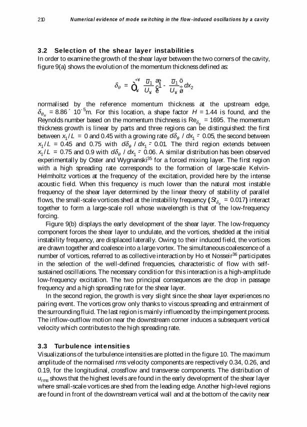
3.2 Selection of the shear layer instabilitiesIn order to examine the growth of the shear layer between the two corners of the cavity,figure 9(a) shows the evolution of the momentum thickness defined as:

normalised by the reference momentum thickness at the upstream edge,m. For this location, a shape factor is found, and the

Reynolds number based on the momentum thichness is . The momentumthickness growth is linear by parts and three regions can be distinguished: the firstbetween and 0.45 with a growing rate , the second between

and 0.75 with . The third region extends betweenand 0.9 with . A similar distribution has been observed

experimentally by Oster and Wygnanski35 for a forced mixing layer. The first regionwith a high spreading rate corresponds to the formation of large-scale Kelvin-Helmholtz vortices at the frequency of the excitation, provided here by the intenseacoustic field. When this frequency is much lower than the natural most instablefrequency of the shear layer determined by the linear theory of stability of parallelflows, the small-scale vortices shed at the instability frequency ( ) interacttogether to form a large-scale roll whose wavelength is that of the low-frequencyforcing.

Figure 9(b) displays the early development of the shear layer. The low-frequencycomponent forces the shear layer to undulate, and the vortices, shedded at the initialinstability frequency, are displaced laterally. Owing to their induced field, the vorticesare drawn together and coalesce into a large vortex. The simultaneous coalescence of anumber of vortices, referred to as collective interaction by Ho et Nosseir36 participatesin the selection of the well-defined frequencies, characteristic of flow with self-sustained oscillations. The necessary condition for this interaction is a high-amplitudelow-frequency excitation. The two principal consequences are the drop in passagefrequency and a high spreading rate for the shear layer.

In the second region, the growth is very slight since the shear layer experiences nopairing event. The vortices grow only thanks to viscous spreading and entrainment ofthe surrounding fluid. The last region is mainly influenced by the impingement process.The inflow-outflow motion near the downstream corner induces a subsequent verticalvelocity which contributes to the high spreading rate.

3.3 Turbulence intensitiesVisualizations of the turbulence intensities are plotted in the figure 10. The maximumamplitude of the normalised velocity components are respectively 0.34, 0.26, and0.19, for the longitudinal, crossflow and transverse components. The distribution of

shows that the highest levels are found in the early development of the shear layerwhere small-scale vortices are shed from the leading edge. Another high-level regionsare found in front of the downstream vertical wall and at the bottom of the cavity near

urms

rms

Stdq= .0 017

d dxdq / ˜1 0 06- .x L1 0 75/ = .d dxdq / ˜1 0 01- .x L1 0 45/ = .

d dxdq / ˜1 0 05- .x L1 0/ =

Redq= 1695

H = .1 44dqR= . ´ -8 86 10 5

dq = -æèç

öø÷-¥

+¥

¥ ¥ò 1 1

21uU

uU

dx


the middle. These two regions mark the beginning and the end of the reverse jet-likeflow in the cavity.

The quantities and are maximum near the downstream corner due to theimpingement process. The high-amplitude region begins after a distance of fromthe leading egde and encompass all the vertical extent further downstream. Theprincipal information from these turbulence intensities is the great unsteadiness of theflow within the cavity, which seems severely coupled to the shear layer. The velocitystress tensor distribution shows high correlation in the shear layer due to theexistence of small-scale structures especially during the first half of its growth. Thepeak value of 0.04 compares well with the measurements of Oster and Wygnanski35

(0.036) for a turbulent mixing layer. This is however greater than the values of Lin andRockwell34 (0.01) or Forestier11 (0.023) for cavity flows. This overestimation maybe associated to the too dissipative effect of the eddy viscosity model in the separatedshear layer and needs further investigation. The interaction with the downstream ismarked by the change of the sign of the stress tensor due to the presence of an importantvertical motion.

3.4 Role of the recirculationFigure 11 shows the velocity vectors associated with the mean velocity in the midplaneof the cavity. A downward deflected flow forms a jet that continues along the bottomof the cavity and is lastly drawn upward toward the separating shear layer at theupstream corner to satisfy entrainment demands.The last two thirds of the cavity exhibita large-scale recirculation bubble, also visible in the instantaneous velocity picturesof figure 8. The averaged pattern is in agreement with the features of the PIV

uvrms

0 5. Dwrmsvrms


Figure 9. (a): Non-dimensional momentum thickness between the twocorners of the cavity; (b): Zoom of velocity field around the upstreamcorner ofthe cavity showing the collectiveinteraction.

- < <( )0 1 1 11. / .x D

d dq q/R

measurements of Lin and Rockwell, where the recirculation occupies the right half of thecavity with an aspect ratio of 2. The upward entrainment flow may influence theinitial development of the shear layer. Lin and Rockwell suggest that the unsteadiness ofthis upward-oriented jet contributes to the modulated character of the separated shearlayer, and thus to the appearance of a low-frequency peak in the pressure spectra nearimpingement. Similarly, the views of figure 8 indicate that a number of admissiblepatterns of the recirculation can occur. In figure 8(d)(e) the swirl pattern encompassesone half of the recirculation, suggesting the possibility of a coupling of the recirculationwith the separated shear layer. Recent bidimensional simulations of Pereira and Sousa37

and Najm and Ghoniem38 address the potential role of the large-scale vortex within thecavity. By viewing this region of the flow as a dynamical system, it is possible to definea mechanism of instability due to the recirculation system.

We must notice that the oscillation components having frequencies lower thanthe fundamental have been found in the spectra of velocity fluctuations in mixing layer-edge (Hussain and Zaman39), cavity (Rockwell and Knisely40,41), and jet-edgeinteractions (Stegen and Karamcheti42), suggesting that there is a well-definedmechanism for generating these components, common to a number of flow geometries.

L D/


Figure 10. Contours for the turbulent intensities: from left to right, and from top

to bottom, (8 isocontours between 0.12 and 0.26 with

interval 0.02), (6 isocontours between 0.12 and 0.22

with interval 0.02), (6 isocontours between 0.12 and

0.22 with interval 0.02), , ( – – –) 12 negativeisocontours between -0.024 and -0.002 with interval 0.002), (——)4 positive isocontours between 0.001 and 0.004 with interval 0.001).

uv u u Urms = ¥1 22’ ’ /

w u Urms = ¥32’ /

v u Urms = ¥22’ /

u u Urms = ¥12’ /

Noting that mixing layer-edge or jet-edge configurations do not involve a recirculatingflow, we can conclude that the recirculating flow is not necessary to induce amodulation of the shear layer.

3.5 Features of the radiated acoustic fieldThe pressure field obtained directly by DNC is plotted in figure 12(a). It shows a strongdownstream directivity due to the convection of acoustic wave fronts by the mean flowcombined with the reflections on the cavity walls. The dominant frequency correspondsto . The pressure spectrum in the near-field (fig. 12(b)) exhibits a low-frequencypeak 12 dB higher than the high-frequency peak. Note that the Schlieren visualizationof Karamcheti for this configuration indicates the predominance of the high component.In the present simulation, the predominance of the lower mode in the shear layerprobably related to the dissipative effect of the viscosity model implies a more violentimpingement of the larger-scale structures upon the downstream corner of the cavity, sothat the lower component is reinforced in the acoustic spectra.

St low


Figure 11. Distribution of averaged velocity inside the cavity in the median plane.

Figure 12. (a) Pressure field from the DNC in the midplane of the cavity (levelsbetween -5000 and 5000 Pa); (b) Spectrum of pressure fluctuations at thelocation indicated by a bullet on the left.

The far-field radiation computed by the extrapolation method is presented infigure 13(a). The extrapolation method is seen to extend well the DNC solution. Theprofiles in the overlapping region, shown in figure 13(b), are in good agreement withthe DNC profiles. The proposed method would be most useful when a large amountof sound field data are needed at not too large distance from the source. For a very long-range propagation, integral methods may still be preferable. In the presentapplication with a high subsonic flow (M = 0.8), the non linear steepening of thewavefronts imposed a relatively fine meshsize to reduce numerical oscillations. For lowerMach number, the wavelengths involved are larger and the propagation would remainlinear, so that the difference between the meshsizes for the acoustic calculation and forthe DNC would be increased.

4. CONCLUSIONThe interaction of a turbulent boundary layer with a cavity, and its radiated field arecomputed using Direct Noise Computation. The reproduction of a configurationinvestigated experimentally by Karamcheti is performed using Large Eddy Simulationto maintain reasonable computational cost. The bypass transition toward realisticturbulence ahead of the cavity is successfully achieved through the superimposition ofrandom Fourier modes on a turbulent mean profile. A method for extending the acousticnear-field to far-field is presented: WNLEE are solved to extent the DNC solution,reducing the cost of the calculation but maintaining a high accuracy.


12

8

10

6

4

2

0

2 12 6 2 4 2 2 0 2 4 6 8

x1 / D

x 2 /

D

4 2 0 2 48000

4000

0

4000

8000

p´ (

Pa)

x1 / D

(a)

(b)

Figure 13. (a): Pressure field obtained by the extrapolation method from theextrapolation surface (shown by the dashed line). The DNC near-field isplotted under the extrapolation surface. Sideview in the median plane.Levels between -5000 and 5000 Pa; (b): Longitudinal pressure profilesalong . (——), DNC and ( – – –), WNLEE.x D2 3 6˜ .-

The principal observation concerning cavity noise is the possibility of switchingbetween mode I and mode II of cavity oscillations. This switching is not random in timebut follows a cycling pattern, with a successive alternance between the two modes, evenif a certain level of intermittency is observed in this succession. In turbulent conditions,the coherent structures adopt the shape of clusters of small scales, and the alternance ofdifferent size of the dominant structures proceed by a reorganisation of these clusters.The examination of the early shear-layer growth reveals that the formation of large-scale structures is possible through a collective interaction after the upstream corner,corresponding to the fusion of a number of smaller vortices shedded at the most instablefrequency of the shear-layer. This phenomenon appears to be of fundamental interest inthe process of selection of the main oscillation frequencies. Another interesting findingis the strong unsteadiness of the recirculating flow within the cavity, which seemsseverely coupled to the shear-layer modulations. However the role of the recirculatingflow on the switching phenomenon is not clear since the coexistence of different modeshas been noticed in the self-sustained oscillations for configurations without adjacentrecirculating flows. The acoustic near-field obtained by the DNC is extended to the far-field by using simplified equations for the acoustic disturbances, and clearly indicatethe predominance of the lower component. In the present simulation, the developmentof the lower mode is promoted by the numerics, so that a more violent impingementupon the downstream corner of the cavity is induced and will dominate the acousticradiation.

ACKNOWLEDGMENTSSupercomputer time is supplied by Institut du Développement et des Ressources enInformatique Scientifique (IDRIS - CNRS).

REFERENCES1. Karamcheti, K., Acoustic radiation from two-dimensional rectangular cutouts in

aerodynamic surfaces. NACA Technical Note 3487, 1955.

2. Colonius, T., Basu, A.J. & Rowley, C.W., Numerical investigation of the flow pasta cavity, AIAA Paper 99-1912, 1999.

3. Shieh, C.M. & Morris, P.J., Parallel computational aeroacoustic simulation ofturbulent subsonic cavity flow, AIAA Paper 2000-1914, 2000.

4. Heo, D.N. & Lee, D.J., Numerical investigation of the cover-plates effects on therectangular open cavity, AIAA Paper 2001-2127, 2001.

5. Gloerfelt, X., Bailly, C. & Juvé, D., Computation of the noise radiated bya subsonic cavity using direct simulation and acoustic analogy, AIAA Paper2001-2226, 2001.

6. Rockwell, D., Oscillations of impinging shear layers, AIAA Journal, 1983, 21(5),p. 645–664.

7. Cattasfesta III, L.N., Garg, S., Kegerise, M.A. & Jones, G.S., Experiments oncompressible flow-induced cavity oscillations, AIAA Paper 98-2912, 1998.


8. Gloerfelt, X., Bailly, C. & Juvé, D., Direct computation of the noise radiated by asubsonic cavity flow and application of integral methods, Journal of Sound andVibration, 2003, 226(1), p. 119–146.

9. Larchevêque, L., Sagaut, P., Mary, I., Labbé, O. & Comte, P., Large-eddy simulationof a compressible flow past a deep cavity, Physics of Fluids, 2003, 15(1), p. 193–210.

10. Gloerfelt, X., Bogey, C., Bailly, C. & Juvé, D., Aerodynamic noise induced bylaminar and turbulent boundary layers over rectangular cavities, AIAA Paper2002-2476, 2002.

11. Forestier, N., Jacquin, L. & Geffroy, P., The mixing layer over a deep cavity athigh-subsonic speed, Journal of Fluid Mechanics, 2003, 475, p. 101–145.

12. Shieh, C.M. & Morris, P.J., Comparison of two- and three-dimensional turbulentcavity flows, AIAA Paper 2001-0511, 2001.

13. Fureby, C. & Grinstein, F.F., Large Eddy Simulation of high-Reynolds numberfree and wall-bounded flows, Journal of Compututational Physics, 2002, 181,p. 68–97.

14. Ahuja, K.K. & Mendoza, J., Effects of cavity dimensions, boundary layer, andtemperature in cavity noise with emphasis on benchmark data to validatecomputational aeroacoustic codes, NASA CR-4653, 1995.

15. Pilon, A.R. & Lyrintzis, A.S., Refraction corrections for the Kirchhoff method,AIAA Paper 97-1654, 1997.

16. Shih, S.H., Hixon, D.R., Mankbadi, R.R., Pilon, A. & Lyrintzis, A., Evaluation offar-field jet noise prediction methods, AIAA Paper 97-0282, 1997.

17. Freund , J.B., Lele , S.K. & Moin , P., Matching of near/far-field equation sets fordirect computations of aerodynamic sound, AIAA Paper 93-4326, 1993.

18. Shih, S.H., Hixon, D.R. & Mankbadi, R.R., A zonal approach for prediction of jetnoise, AIAA Paper 95-144, 1995.

19. Deardorff, J.W., A numerical study of three-dimensional turbulent channel flow atlarge Reynolds numbers, Journal of Fluid Mechanics, 1970, 41(2), p. 453–480.

20. Erlebacher, G., Hussaini, M.Y., Speziale, C.G. & Zang, T.A., Toward the large-eddy simulation of compressible turbulent flows, Journal of Fluid Mechanics,1992, 238, p. 155–185.

21. Moin, P. & Kim, J., Numerical investigation of turbulent channel flow, Journal ofFluid Mechanics, 1982, 118, p. 341–377.

22. Bogey, C. & Bailly, C., A family of low dispersive and low dissipative explicitschemes for computing aerodynamic noise, AIAA Paper 2002-2509, 2002.

23. Bogey, C. & Bailly, C., Three-dimensional non-reflective boundary conditions foracoustic simulations: far field formulation and validation test cases, ActaAcustica, 2002, 88, p. 463–471.

24. Tam, C.K.W. & Dong, Z., Advances in numerical boundary conditions forcomputational aeroacoustics, Journal of Computational Acoustics, 1999, 6(4),p. 377–402 (or AIAA Paper 97-1774).


25. Rai, M.M. & Moin, P., Direct numerical simulation of transition and turbulence ina spatially evolving boundary layer, Journal of Computational Physics, 1993,109, p. 169–192.

26. Ducros, F., Comte, P. & Lesieur, M., Large-eddy simulation of transition toturbulence in a boundary layer developing spatially over a flat plate, Journal ofFluid Mechanics, 1996, 326, p. 1–36.

27. Voke, P.R. & Yang, Z., Numerical study of bypass transition, Physics of Fluids,1995, 7(9), p. 2256–2264.

28. Bailly, C., Lafon, P. & Candel, S., A stochastic approach to compute noisegeneration and radiation of free turbulent flows, AIAA Paper 95-092, 1995.

29. Spalart, P.R., Direct simulation of a turbulent boundary layer up to ,Journal of Fluid Mechanics, 1988, 187, p. 61–98.

30. Head, M.R. & Bandyopadhyay, P., New aspects of turbulent boundary layerstructures, Journal of Fluid Mechanics, 1981, 107, p. 297–338.

31. Bogey, C. & Bailly, C., LES of a high Reynolds, high subsonic jet: Effects of thesubgrid modellings on flow and noise, AIAA Paper 2003-3557, 2003.

32. Whitham, G.B., Linear and nonlinear waves, Wiley, New York, 1974, p. 312–338. 33. Tang, Y.-P. & Rockwell, D., Instantaneous pressure fields at a corner associated

with vortex impingement, Journal of Fluid Mechanics, 1983, 126, p. 187–204. 34. Lin, J.C. & Rockwell, D., Organized oscillations of initially turbulent flow past a

cavity, AIAA Journal, 2001, 39(6), p. 1139–1151.

35. Oster, D. & Wygnanski, I., The forced mixing layer between parallel streams,Journal of Fluid Mechanics, 1982, 123, p. 91–130.

36. Ho, C.-M. & Nosseir, N.S., Dynamics of an impinging jet. Part 1. The feedbackphenomenon, Journal of Fluid Mechanics, 1981, 105, p. 119–142.

37. Pereira, J.C.F. & Sousa, J.M.M., Experimental and numerical investigation offlow oscillations in a rectangular cavity, ASME Journal of Fluids Engineering,1995, 117, p. 68–74.

38. Najm, H.N. & Ghoniem, A.F., Numerical simulation of the convective instabilityin a dump combustor, AIAA Journal, 1991, 29(6), p. 911–919.

39. Hussain, A.K.M.F. & Zaman, K.B.M.Q., The free shear layer tone phenomenonand probe interference, Journal of Fluid Mechanics, 1978, 87(2), p. 349–383.

40. Rockwell, D. & Knisely, C., Vortex-edge interaction: Mechanisms for generatinglow frequency components, Physics of Fluids, 1980, 23(2), p. 239–240.

41. Knisely, C. & Rockwell, D., Self-sustained low frequency components in animpinging shear layer, Journal of Fluid Mechanics, 1982, 116, p. 157–186.

42. Stegen, G.R. & Karamcheti, K., Multiple tone operation of edgetones, Journal ofSound and Vibration, 1970, 12(3), p. 281–284.

Redq= 1410


numerical evidence of mode switching in the flow-induced...

Documents