Noname manuscript No.(will be inserted by the editor)

Numerical integration of polynomials and discontinuous functions on irregularconvex polygons and polyhedrons

S. E. Mousavi · N. Sukumar

Received: date / Accepted: date

Abstract We construct efficient quadratures for the integration of polynomials over irregular convex polygons and

polyhedrons based on moment fitting equations. The quadrature construction scheme involves the integration of

monomial basis functions, which is performed using homogeneous quadratures with minimal number of integration

points, and the solution of a small linear system of equations. The construction of homogeneous quadratures is

based on Lasserre’s method for the integration of homogeneous functions over convex polytopes. We also construct

quadratures for the integration of discontinuous functions without the need to partition the domain into triangles

or tetrahedrons. Several examples in two and three dimensions are presented that demonstrate the accuracy and

versatility of the proposed method.

Keywords numerical integration · Lasserre’s method · Euler’s homogeneous function theorem · irregular polygons

and polyhedrons · homogeneous and nonhomogeneous functions · strong and weak discontinuities · polygonal finite

elements · extended finite element method.

1 Introduction

Numerical integration is an important ingredient within many solution techniques in engineering and the sciences.

With the development of new numerical methods, the need for accurate and efficient integration schemes has em-

anated, due to both the general shapes of the integration domain and the presence of generalized classes of functions.

Conforming polygonal finite elements [1–4] and finite elements on convex polyhedra [5–7] require the integration of

non-polynomial basis functions. The integration of polynomials on irregular polytopes arises in the non-conforming

variable-element-topology finite element method [8, 9], discontinuous Galerkin finite elements [10], finite volume ele-

ment method [11] and mimetic finite difference schemes [12–14]. In partition-of-unity methods such as the extended

finite element method (X-FEM) [15, 16], discontinuous functions are integrated to form the stiffness matrix of el-

ements that are cut by a crack or an interface. Versatility of such methods is due to their power to handle more

complicated internal geometries, albeit at the expense of greater demands on numerical integration, which points to

the need for devising flexible and efficient numerical integration techniques.

In this paper, we focus on the integration of polynomials on irregular convex polygons and polyhedra. In two

dimensions, the boundaries of the integration region are contained in straight lines and in three dimensions, the domain

is bounded by planes. Also, we are particularly interested in cases where the integrand is not known explicitly, but

can be evaluated at any point within the domain of integration. Such cases arise in finite-element and partition-

of-unity methods. There are few choices for the integration of polynomials over general two- and three-dimensional

regions. Most of the available methods in the literature are appropriate for special forms of polynomials [17–19], or

are restricted to the integration on simplexes and regular polytopes [20–22]. The most frequently used strategy for the

integration of a polynomial over an irregular polygon or polyhedron is to decompose it into triangles or tetrahedrons

and apply well-known integration rules to each partition. Integration of polynomials over n-dimensional polyhedra

can also be done by lower-dimensional integrations over the boundary of the domain using divergence theorem and/or

National Science Foundation, CMMI-0626481, DMS-0811025.

S. E. Mousavi · N. SukumarDepartment of Civil and Environmental Engineering, University of California, Davis, CA 95616. E-mail: nsukumar@ucdavis.edu

2

Green’s theorem [23–28], or using Euler’s theorem in case of homogeneous functions [17, 18]. A method is presented

in Reference [19] for the efficient integration of powers of linear forms over simplexes in very high dimensions.

In this paper, we use moment fitting equations to construct quadrature rules for the integration of polynomials

on irregular convex polygons and polyhedra. The moment fitting technique is independent of the shape of the domain

or type of the basis functions, and enables one to construct integration rules with desirable properties, such as

interiority of points and symmetry. These properties are enforced through adding appropriate constraints to the

moment equations. In Reference [29], moment fitting was used together with the node elimination algorithm [30], to

construct and optimize quadratures for the integration of polynomials over arbitrary polygons. The moment equations

contain the integration of the basis functions (polynomials of total degree up to d) over the domain. These integrations

were performed algebraically in Reference [29]. Although algebraic integration of polynomials is straightforward in

two dimensions, it is not generally a well-posed problem in three dimensions, and therefore extending the technique

of Reference [29] to three dimensions is unwieldy. It bears mention that for monomials one can use divergence

theorem to transform the surface integrals to line integrals [8], which can be handled efficiently. In three dimensions,

successive application of the divergence theorem results in line integrals over the edges of the polyhedron [9, 26, 28].

Lasserre’s method [17, 18], which is a technique for the integration of homogeneous functions on convex polygons and

polyhedra based on Euler’s theorem, transforms the integration of a homogeneous function on a convex polygon to line

integrations over its edges. Similarly, one can apply the technique twice for the integration over a convex polyhedron

and transform the volume integrals into line integrals. Lasserre’s formula has advantages over the divergence theorem:

calculation of the normals to the boundary and projections on the plane are not required and the integrand remains

unchanged. The basis functions of the moment fitting equations are monomials with respect to the spatial coordinates,

which makes Lasserre’s method ideal for their integration.

The structure of this paper is as follows. Lasserre’s method for the integration of homogeneous functions is ex-

plained and the main theorems are presented in Section 2.1. A method for constructing quadratures for the integration

of homogeneous functions based on Lasserre’s method is presented in Section 2.2. These homogeneous quadratures

are used throughout the paper for the integration of the basis functions. In Section 2.3, we propose a technique for

the integration of a linear combination of homogeneous functions, when the function is not known explicitly, based

on Lasserre’s method and the solution of a small system of linear equations. We describe the algorithm for the con-

struction of quadratures for irregular convex polygons in Section 3, followed by several examples. In Section 4, we

consider the integration of functions with strong and weak discontinuities and demonstrate the applicability of the

method through a few examples. We extend the quadrature construction scheme to three dimensions in Section 5,

both for polynomial functions and discontinuous functions. We integrate a cubic polynomial on a convex polyhedron

and present two practical examples that arise in crack-modeling using the X-FEM. The main findings of this study

are summarized and some concluding remarks are made in Section 6.

2 Lasserre’s method for integration of homogeneous functions

2.1 Lasserre’s method

Lasserre presented a method for the integration of positively homogeneous functions over convex polytopes [17, 18].

Integration in Ω ⊂ Rn is reduced to a number of weighted integrations over the (n − 1)-dimensional faces of Ω,

i.e., Ωi ⊂ Rn−1 for i = 1, 2, . . . , m, through the application of Euler’s theorem. The weights of the integrations are

functions of the geometry of Ω and the degree of homogeneity. The integrations in (n − 1) dimensions can be done

using standard integration schemes in an efficient way. Under certain circumstances the reduction of the integrations

to even lower dimensions is also possible.

Let f : Rn → R be a real continuous positively homogeneous function of degree q, f(λx) = λqf(x) for all λ > 0

and x ∈ Rn. Moreover, assume that the domain of integration Ω ⊂ Rn is a convex polytope, which is described as

x ∈ Rn : Ax ≤ b, with A a real m×n matrix and b a real vector of length m. Also, let Ωi be the (n−1)-dimensional

face of Ω : Ωi = x ∈ Rn : Ax ≤ b,Aix = bi is determined by the hyperplane Aix = bi with Ai being the ith

row of A. The face Ωi is contained in the (n− 1)-dimensional variety1 Hi and the algebraic distance from the point

x0 to Hi is denoted by d(x0,Hi) and can be calculated as d(x0,Hi) = (bi − Aix0)/ ‖ Ai ‖, with ‖ · ‖ denoting

the Euclidean norm. The following theorems from Reference [17] describe the method. These theorems are based on

Euler’s homogeneous function theorem, namely

qf(x) = <∇f(x),x> ∀x, (1)

1 A variety is the extension of the algebraic curves to higher dimensions, or more precisely, a set of points that satisfy asystem of polynomial equations.

3

where f is a continuously differentiable function and < · , ·> denotes the inner product of vectors.

Remark: Throughout this paper, we will interchangeably use the tensor representation of coordinates xi3i=1, and

the Cartesian representation x, y, z.

Theorem 1 (Integration of homogeneous functions) Assume that f is continuously differentiable, Vn(Ω) 6= 0,

and for all i = 1, . . . , m, Vn−1(Ωi) 6= 0. ThenZΩ

f(x)dx =1

n + q

mXi=1

bi

‖ Ai ‖

ZΩi

fdµ =

mXi=1

d(o,Hi)

n + q

ZΩi

fdµ, (2)

where dµ is the Lebesgue measure on the (n− 1)-dimensional affine variety Hi that contains Ωi (dµ =‖ Ai ‖ dx) and

o is the origin. Vn and Vn−1 denote the n- and (n− 1)-dimensional volume, respectively.

Theorem 2 (Further reduction of integration of homogeneous functions) Let f be twice continuously dif-

ferentiable and for all i = 1, . . . , m, either Ωi = ∅ or Vn−1(Ωi) 6= 0. Also, assume that for every j = 1, . . . , m, j 6= i,

either Ωij = ∅ or Vn−2(Ωij) 6= 0. Then

ZΩi

fdµ =1

n + q − 1

24Xj 6=i

di(x0,Hij)

ZΩij

fdν +

ZΩi

<∇f,x0 > dµ

35 , (3)

where Ωij is the (n− 2)-dimensional face of Ω defined as Ωij = x ∈ Ω,Aix = bi,Ajx = bj, and Hij is the affine

variety that contains Ωij . For example, in two dimensions with Ω being a polygon, Ωi is the ith edge and Ωij is the

vertex of the polygon connecting edges i and j. In three dimensions, Ωi is the ith face of the polytope and Ωij is the

line segment at the intersection of faces i and j. dν is the Lebesgue measure on the (n− 2)-dimensional affine variety

Hij ⊂ Hi, and x0 ∈ Hi is a fixed point that can be selected arbitrarily.

In Section 2.2, we construct quadrature rules based on Theorem 1 with the quadrature points on the faces of

the integration region. The resulting quadratures are suitable for the integration of homogeneous functions. In two

dimensions, the faces of the region are line segments. Hence, these quadratures reduce the area integration to line

integrations. The integration can be further reduced to function evaluation at polygonal vertices using Theorem 2.

However, this is avoided since optimal one-dimensional Gauss quadrature rules are available. In three dimensions,

we use the above theorems to reduce the volume integrals to line integrals and then apply one-dimensional Gauss

quadrature rules.

2.2 Quadratures for homogeneous functions

Theorem 1 can be used to construct quadrature rules for the integration of homogeneous functions over the integration

region Ω with all the integration points located on the faces of the region Ωi. Assume that Qi is a nspi-point

quadrature over Ωi with the integration points and weights xai , wa

i nspi

a=1 and define the operation of Qi on a function

f as:

Qi(f) =

nspiXa=1

wai f(xa

i ) ≈Z

Ωi

fdµ. (4)

Now, obtain the modified quadrature Qi with points and weights xai , wa

i nspi

a=1 using:

xai = xa

i , wai = d(o,Hi)w

ai . (5)

The combination of the quadrature rules Q = Qimi=1 constructed over the m faces of Ω, is a quadrature, with

nsp =Pm

i=1 nspi integration points on the faces of the domain, that can integrate q-homogeneous functions over the

integration region:

Q(f) ≈ (n + q)

ZΩ

f(x)dx. (6)

We will refer to such quadratures as homogeneous quadratures throughout this paper, since they can only be used to

integrate homogeneous functions. For example, in a two-dimensional setting, with Ω being a convex m-gon and Ωi

denoting the ith edge of the polygon, one can obtain Qi—a standard Gauss quadrature rule over the interval [−1, 1]

is mapped to the line-segment Ωi and the weights of the quadrature are multiplied by the length of the ith edge of

the polygon divided by two.

4

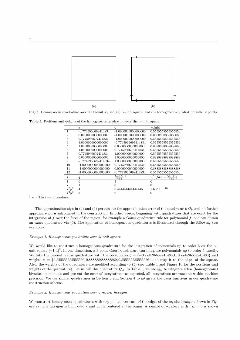
(a) (b)

Fig. 1 Homogeneous quadrature over the bi-unit square. (a) bi-unit square; and (b) homogeneous quadrature with 12 points.

Table 1 Positions and weights of the homogeneous quadrature over the bi-unit square.

x y weight1 -0.7745966692414834 -1.0000000000000000 0.55555555555555562 0.0000000000000000 -1.0000000000000000 0.88888888888888883 0.7745966692414834 -1.0000000000000000 0.55555555555555564 1.0000000000000000 -0.7745966692414834 0.55555555555555565 1.0000000000000000 0.0000000000000000 0.88888888888888886 1.0000000000000000 0.7745966692414834 0.55555555555555567 0.7745966692414834 1.0000000000000000 0.55555555555555568 0.0000000000000000 1.0000000000000000 0.88888888888888889 -0.7745966692414834 1.0000000000000000 0.555555555555555610 -1.0000000000000000 0.7745966692414834 0.555555555555555611 -1.0000000000000000 0.0000000000000000 0.888888888888888812 -1.0000000000000000 -0.7745966692414834 0.5555555555555556

f qQ2(f)n+q

† |R

2 fdA − Q2(f)n+q

| †

1 0 4 0x 1 0 0x2y2 4 0.444444444444445 1.6 × 10−16

x2y3 5 0 0† n = 2 in two dimensions.

The approximation sign in (4) and (6) pertains to the approximation error of the quadratures Qi, and no further

approximation is introduced in the construction. In other words, beginning with quadratures that are exact for the

integration of f over the faces of the region, for example a Gauss quadrature rule for polynomial f , one can obtain

an exact quadrature via (6). The application of homogeneous quadratures is illustrated through the following two

examples.

Example 1: Homogeneous quadrature over bi-unit square

We would like to construct a homogeneous quadrature for the integration of monomials up to order 5 on the bi-

unit square [−1, 1]2. In one dimension, a 3-point Gauss quadrature can integrate polynomials up to order 5 exactly.

We take the 3-point Gauss quadrature with the coordinates ξ = −0.774596669241483, 0, 0.774596669241483 and

weights w = 0.555555555555556, 0.888888888888889, 0.555555555555556 and map it to the edges of the square.

Also, the weights of the quadrature are modified according to (5) (see Table 1 and Figure 1b for the positions and

weights of the quadrature). Let us call this quadrature Q2. In Table 1, we use Q2 to integrate a few (homogeneous)

bivariate monomials and present the error of integration—as expected, all integrations are exact to within machine

precision. We use similar quadratures in Section 3 and Section 4 to integrate the basis functions in our quadrature

construction scheme.

Example 2: Homogeneous quadrature over a regular hexagon

We construct homogeneous quadratures with nsp points over each of the edges of the regular hexagon shown in Fig-

ure 2a. The hexagon is built over a unit circle centered at the origin. A sample quadrature with nsp = 5 is shown

5

(a) (b) (c)

Fig. 2 Homogeneous quadrature over regular hexagon. (a) regular hexagon on a unit circle; (b) homogeneous quadrature with30 points; and (c) relative error of calculating

R7 1/rα dA using homogeneous quadratures.

in Figure 2b. The aim is to integrate f(r) = 1/rα over the regular hexagon, with r being the distance from the origin.

The function 1/rα is homogeneous with degree of homogeneity −α. Since the domain of integration contains the

origin, the integrand is weakly singular, and domain integration using standard quadratures over the triangle requires

many integration points to obtain the desired accuracy. To calculate the reference solution, we use the generalized

Duffy transformation [31] after partitioning the hexagon into 6 triangles by connecting the origin to the vertices of

the hexagon. We increase nsp so that the result approaches the reference value—the efficiency of the method for

f(r) = 1/√

r and f(r) = 1/r is demonstrated in Figure 2c.

The above technique for finding Q is straightforward and provides flexibility when the integrand is homogeneous.

For example, in the node elimination algorithm [29, 30, 32], the basis functions can be selected as monomials that are

homogeneous functions (see Section 3). However, when the integrand is a linear combination of homogeneous functions,

each of the terms must be known explicitly so that they can be integrated separately. This limitation renders the

homogeneous quadratures impractical for finite-element or boundary-element methods, where the integrands are

known implicitly and can only be evaluated at given points. To clarify this issue, let g(x) =P

j gj(x), with gj being

qj-homogeneous. The following integral is valid:ZΩ

g(x)dx ≈X

j

Q(gj)

n + qj, (7)

where Q is the quadrature obtained through (5). If each gj(x) is not known explicitly, then the value of the integral

in (7) can not be computed. In the next section, a solution is devised for this problem.

2.3 Application of Lasserre’s method for the integration of a linear combination of homogeneous functions

Lasserre’s method of integration is an elegant technique for the integration over convex regions. However, the technique

and the corresponding quadrature rules (see Section 2.2) are limited to homogeneous functions. In the case of a linear

combination of homogeneous functions, additional information is required to apply the method: each of the terms in

the sum must be known explicitly and integration is performed for each term individually. In this section, we use the

homogeneous quadratures for the integration of a linear combination of homogeneous functions without knowing or

evaluating each one of them separately.

Assume that Q is a homogeneous quadrature that can integrate a class of functions Φ over the region Ω ⊂ Rn

using (6). Also assume that g(x) can be written as the sum of m homogeneous functions: g(x) =Pm

i=1 gi(x), with

gi ∈ Φ being qi-homogeneous, gi(λx) = λqigi(x) for all λ ∈ R, λ > 0. Note that gi can be the summation of a group

of qi-homogeneous functions (can contain more than one term). We also assume that g is well-defined everywhere in

Rn and can be evaluated even outside the region Ω. One can use (7) to integrate g over the domain, provided that

gimi=1 are known individually. Here we assume that g can only be evaluated at certain points (quadrature points)

and the functions gi are not given; nor do we wish to approximate g explicitly with a few homogeneous functions.

6

According to the definition of homogeneity, and by writing the integration of a sum as the sum of integrals, the

following is valid: ZΩ

g(λx)dx =

ZΩ

mXi=1

gi(λx) =

mXi=1

λqi

ZΩ

gi(x)dx. (8)

Also, the operation of Q on g can be simplified as:

Q(g) = Q(

mXi=1

gi) =

mXi=1

Q(gi) =

mXi=1

(qi + n)

ZΩ

gi(x)dx, (9)

where (6) was used in the derivation of the last term. By exploiting the homogeneity of gi, one can write:

Q(g(λx)) =

mXi=1

λqi(qi + n)

ZΩ

gi(x)dx. (10)

The term on left-hand-side of (10) can be evaluated by manipulating the positions of the integration points of Q:

Q(g(λx)) =Pnsp

i=1 wig(λxi) where xi, winspi=1 are the integration points and weights of Q. Consider a new quadrature

Qλ whose points and weights are defined as xλi = λxi, w

λi = winsp

i=1. Then, one can write:

Q(g(λx)) = Qλ(g(x)). (11)

We arrive at the final equation by substituting (11) into (10) and replacing the integralsRΩ gidx with Ii:

Qλ(g) =

mXi=1

λqi(qi + n)Ii. (12)

Equation (12) has m unknowns Iimi=1, and holds for any given λ > 0. It is straightforward to transform (12) into a

linear system of equations by selecting m values for λ and evaluating the left-hand-side for each of them, as follows:

0BBBB@Qλ1(g)

Qλ2(g)...

Qλm(g)

1CCCCA=

0BBB@λq1

1 (q1 + n) λq21 (q2 + n) . . . λqm

1 (qm + n)

λq12 (q1 + n) λq2

2 (q2 + n) . . . λqm

2 (qm + n)...

......

...

λq1m(q1 + n) λq2

m(q2 + n) . . . λqmm (qm + n)

1CCCA0BBB@

I1I2...

Im

1CCCA . (13)

Once (13) is solved and the unknowns Ii are found, the integration of g follows asRΩ g(x)dx =

Pmi=1 Ii. The square

matrix of coefficients in (13) depends on the degree of homogeneity of gi and the m assumed values for λi, and the

left-hand-side contains the operation of nsp-point quadratures Qλi on the function g—no evaluation of gi is required.

The quadrature construction algorithm in Section 2.2 is applied only once: when Q is created, Qλi are obtained

through the modification of the points of Q.

Example

Consider the numerical integration of g(x, y) = 1 + x2 + y2 − 2y3 over the unit square Ω = [0, 1]2. g contains

homogeneous functions g1 = 1, g2 = x2+y2 and g3 = −2y3, with the degrees of homogeneity of 0, 2 and 3, respectively.

For the sake of illustration, we select the degrees of homogeneity to be q1 = 0, q2 = 1, q3 = 2, q4 = 3, and assume

λ1 = 1/4, λ2 = 1/2, λ3 = 3/4 and λ4 = 1. Using the above algorithm, we obtain: I1 = 1.000000000000000, I2 =

0.000000000000003, I3 = 0.666666666666662, I4 = −0.499999999999998, and I =P4

i=1 Ii = 1.166666666666667,

which agrees with the exact integration of g over the domain. Notice that I2 = 3× 10−15 is consistent with the fact

that there is no term in g with degree of homogeneity of 1.

7

3 Algorithm for the construction of quadratures on irregular convex polygons

3.1 Moment fitting equations

A standard and well-known method for the construction of quadrature rules is the moment fitting equation [33–35]

in which a quadrature is constructed for a class of basis functions over a fixed domain and a given weight function

by solving the moment equation:0BBB@RΩ ω(x)φ1(x) dxRΩ ω(x)φ2(x) dx

...RΩ ω(x)φm(x) dx

1CCCA=

0BBB@φ1(x1) φ1(x2) . . . φ1(xn)

φ2(x1) φ2(x2) . . . φ2(xn)...

......

...

φm(x1) φm(x2) . . . φm(xn)

1CCCA0BBB@

w1

w2

...

wn

1CCCA , (14)

where ω is the weight function, and Φ = φjmj=1 is the set of the basis functions defined over the domain of integration

Ω. The points of the quadrature and the corresponding weights, xi, wini=1, are the unknowns that may be solved for

algebraically or numerically so that the m moment equations are satisfied. The resulting quadrature is exact (within

the tolerance of the solution method) for the integration of the basis functions. The minimum number of integration

points that can satisfy (14) is a classical problem of numerical analysis which has no solution yet [30]. Each integration

point in n-dimensions, contributes n + 1 unknowns (degrees of freedom): n unknowns for its coordinate components

and one for the weight. It can be seen that m/(n + 1) can serve as an estimate for the number of points required to

integrate m basis functions in n dimensions.

Wandzura and Xiao [36] and Xiao and Gimbutas [30] applied Newton’s least squares method to numerically

solve (14) for the construction of high-order quadrature rules over the triangle, the square and the cube and then

proposed the node elimination algorithm—one of the integration points was removed and (14) was solved again to get

a quadrature with one fewer integration point. This procedure was continued until convergence of Newton’s method

could not be achieved anymore. Mousavi et al. [29] employed the node elimination algorithm to build symmetric

quadratures for regular n-gons with n = 5, 6, 7 and 8. They also showed that the method is not restricted to regular

domains—moderate degree close-to-minimal quadrature rules were produced over arbitrary convex and concave poly-

gons. Node elimination algorithm was also used for the integration of discontinuous functions by replacing the weight

function with a step function [32]. A nice feature of the node elimination algorithm is that the Newton iterations are

only for the optimization of the quadrature rule and the output of each iteration is a solution of (14) by construction.

One can stop the iterations as soon as the acquired quadrature is deemed suitable. In this paper, we fix the positions

of the integration points over an irregular polygon and find the corresponding weights by solving (14). On knowing

the locations of the integration points a priori, (14) turns into a linear system of m moment equations and n unknown

weights. In general, the matrix of coefficients Aji = φj(xi) can be non-square and we solve it in a least squares sense,

that is, a solution with the minimum norm is sought. Solutions with some zeros are more desirable, because they

imply fewer number of integration points.

Construction of a quadrature by moment fitting involves a one time calculation of the left-hand-side (lhs) of (14)

that can be done algebraically (the integration boundaries are piecewise analytical curves) or numerically, using

standard integration schemes such as Gauss quadrature rules. Divergence theorem can also be applied to convert

the domain integrals into boundary integrals that can be carried out in a more straightforward manner [8, 9]. In

two dimensions, when the goal is to produce a quadrature for the integration of polynomials of order d or lower,

the set of basis functions Φ includes all bivariate monomials up to order d, Pd = xiyj , i, j ∈ Z, i + j ≤ d. Note

that Pd contains homogeneous functions and the method described in Section 2 can be applied to calculate lhs.

Moreover, Φ can take on the form of any other set of basis functions that are linearly independent and cover the

space of polynomials up to order d. For example, one may start with the monomials Pd and orthogonalize them for

the given weight function over the integration region via a Gram-Schmidt procedure [29, 30]. It bears mention that

the integration of the orthogonal polynomials can be done using integration of homogeneous functions, of course with

some extra steps.

3.2 Description of the algorithm and examples

In this section, we explain the algorithm for the construction of quadrature rules with polynomial-precision on irregular

convex polygons. Consider the quadrilateral shown in Figure 3a. We will construct a quintic quadrature using the

moment fitting equations to illustrate the algorithm. The basis functions in (14) consist of bivariate monomials

xiyj , i+ j ≤ 5 (21 basis functions), with the weight function ω set to unity. Therefore, we need a quadrature that can

8

integrate polynomials of total order up to 5 to calculate the lhs. In one dimension, for example along the polygon

edges, a 3-point Gauss quadrature rule is sufficient for the integration of polynomials up to order 5. Following the

description provided in Section 2.2, a quadrature rule with 12 points is created with all the points lying along the

edges (see Figure 3b). This rule can integrate the basis functions using (6) and is then adopted to calculate the lhs

of (14). Having 21 equations to satisfy in (14), it is reasonable to expect at least 21 unknowns—there should be

at least 21 integration points. For the locations of the integration points, we find the centroid of the polygon and

connect it to the vertices and the middle of the edges and then pick 3 points over each of them (Figure 3c). After

solving the moment equations using a least squares fitting, 21 non-zero weights are obtained, corresponding to 21

integration points: this is a quadrature rule that can integrate polynomials of total order up to 5 over the polygon

(see Figure 3d). The positions of the integration points can be selected differently: for example, as a combination of

the polygonal vertices using a barycentric coordinate with random coefficients (Figure 3e). In Figure 3f, a mesh-grid

over the box containing the quadrilateral is constructed and the points that fall inside the domain are used as the

integration points. The three quadratures shown in Figures 3d to 3f, have 21 points and integrate polynomials of

order 5 over the quadrangle. We calculate the relative norm of the quadrature error (called relative error from now

on) as

ErelQ =

‖ I(Φ)−Q(Φ) ‖‖ I(Φ) ‖ , (15)

where, Φ is the set of numf basis functions and I(Φ) and Q(Φ) are vectors of length numf with Ii =RΩ φidx and

Qi = Q(φi). The relative error of these quadratures is of order 10−16. Some of the weights of the integration points

are negative.

To show the versatility of the approach, we construct quadrature rules of orders 3, 5 and 7 over irregular convex

polygons with 4, 6, 8, 10, 11 and 12 number of vertices (see Figure 4). Figures 4a to 4f present quadratures of

order 3 with the position of the integration points determined using diagonals and bisectors of the polygon, as

shown in Figure 3c. In two dimensions, there are 10 monomials in the space of polynomials up to order 3. Hence,

10 integration points are expected and realized, with the exception of the bi-unit square in Figure 4a, which is a

special case and fewer points are obtained. This can be explained in light of the symmetry of the square and the

quadrature—the integral of many of the basis functions is identically equal to zero, which is satisfied by choosing

a symmetric quadrature. The relative error of the quadrature in all these examples is of order 10−16. Figures 4g

to 4` show quadrature rules of order 5 with random distribution of integration points. The relative error of the

quadrature in this case is of order 10−13, which can be attributed to the poor distribution of the points. One can

choose points that are more evenly distributed, e.g., by selecting a larger ensemble of random points. However, this

increases the computation of the matrix of coefficients Aji in (14). We simply modified the random coefficients so

that the integration points are attracted towards the polygon vertices and edges: the results are shown in Figures 4m

to 4r for order 5 quadratures. The relative norm of the quadrature error is reduced to the order of 10−15 as a result

of better distribution of the integration points. This reveals the important effect of the locations of the integration

points on the accuracy of the quadrature; at the same time, it indicates that one has the freedom of placing the points

at certain locations of interest at the expense of losing some accuracy. Figures 4s to 4x pertain to order 7 quadratures

with mesh-grid distribution of integration points, with the relative norm of error of order 10−15. The lower accuracy

of the quadrature is due to the ill-conditioning of the matrix of coefficients. The number of integration points for

quadratures of order 5 and 7 are 21 and 36, respectively, which is equal to the number of basis functions in each case.

4 Quadratures for discontinuous functions

In many applications of numerical methods, the integrand may contain a discontinuity over the domain of integra-

tion. For example, such is the case in partition-of-unity methods like the extended finite element method for modeling

cracks [15] and material interfaces [16]. Two different types of discontinuity exist in these applications: weak discon-

tinuity, where the derivative of a continuous function is discontinuous, e.g., |x|; and strong discontinuity, where the

function itself is discontinuous, e.g., the generalized Heaviside function. A technique will be presented in the following

sections to construct quadratures for handling strong and weak discontinuities. For some of the existing methods for

integrating discontinuous functions, see References [32, 37–39].

4.1 Strong discontinuities

In this section, we construct efficient quadrature rules that can integrate discontinuous functions without partition-

ing the domain. For this purpose, similar to Reference [32], we solve the moment equations (14) over the entire

9

(a) (b) (c)

(d) (e) (f)

Fig. 3 Algorithm for the construction of a quadrature for an irregular convex polygon. (a) domain of integration; (b) homo-geneous quadrature for the integration of basis functions; (c) locations of integration points (25 points); (d) final quadratureover the quadrilateral (21 points, relative norm of quadrature error = 4×10−16); (e) locations of integration points are randomcombination of the polygonal vertices using barycentric coordinates (21 points, relative norm of quadrature error = 7× 10−16);(f) locations of integration points are selected as the grid points over a box containing the polygon (21 points, relative norm ofquadrature error = 1 × 10−16).

domain after replacing the weight function with a discontinuous function. The difference between our method and

the technique presented in Reference [32] is two-fold: (1) we evaluate the lhs of (14) using homogeneous quadratures

presented in this paper, which results in fast and efficient evaluation of the integrals; and (2) we fix the locations

of the integration points and solve a linear system of equations to obtain the corresponding weights. The number of

integration points numx is proportional to the number of basis functions numf present in the moment equations

(numx ∝ numf), and is not affected by the shape of the domain or the configuration of the discontinuity. A node

elimination algorithm can still be applied to the final quadrature to reduce the number of integration points (in this

case, one will have numx ∝ numf/(n + 1) in Rn), with the additional cost of optimization iterations. We will skip

this step in the quadrature construction scheme presented here.

The algorithm for the construction of a discontinuous quadrature is similar to the one presented in Section 3.2

for polynomials, except that the weight function is set to the generalized Heaviside function and the lhs of (14) is

evaluated differently. We explain this step through an illustrative example. Consider an irregular convex polygon

with the discontinuity shown in Figure 5a. The generalized Heaviside function assumes a value of +1 above the

discontinuity (in Ω+) and −1 below the discontinuity (in Ω−). We intend to create a discontinuous quadrature Qd

over Ω = Ω+ ∪Ω− so that

Qd(f(x)) =

ZΩ

f(x)H(x)dx =

ZΩ+

f(x)dx−Z

Ω−f(x)dx, (16)

where f ∈ Pd is any bivariate polynomial of total order up to d. Therefore, the basis functions include all bivariate

monomials up to order d, i.e., the set of numf = (d + 1)(d + 2)/2 functions xiyj , i + j ≤ d. To calculate the lhs

of (14), we construct two homogeneous quadrature rules according to Section 2.2: QΩ+ over Ω+ and QΩ− over Ω−

(see Figures 5b and 5c, respectively). The specific combination of these quadratures QΩ± = xi, wi,xj ,−wj with

xi, wi being the points and weights of QΩ+ and xj , wj, the points and weights of QΩ− , is used to evaluate

10

(a)

(b)

(c)

(d)

(e)

(f)

(g)

(h)

(i)

(j)

(k)

(`)

(m)

(n)

(o)

(p)

(q)

(r)

(s)

(t)

(u)

(v)

(w)

(x)

Fig. 4 Examples of quadratures for irregular convex polygons with 4, 6, 8, 10, 11 and 12 vertices. (a)-(f) order 3, uniformdistribution of points as described in Section 3.2, relative norm of quadrature error of order 10−16; (g)-(`) order 5, randomdistribution of points, relative norm of quadrature error of order 10−13; (m)-(r) order 5, random distribution of points bymanipulating the coefficients, relative norm of quadrature error of order 10−15; (s)-(x) order 7, locations of integration pointsare selected from a mesh-grid over the polygon, relative norm of quadrature error of order 10−15.

11

lhs of (14) when the weight function ω(x) is set to H(x). Once the lhs is calculated, the rest of the steps in the

quadrature construction is similar to those for the integration of polynomials. See Figures 5d and 5e for the final

quadrature when the integration points are selected randomly and over a uniform grid, respectively. In this example,

we construct a third-order quadrature rule with the points and weights given in Table 2. Also, we calculate the

integration of bivariate monomials multiplied by the generalized Heaviside function and compare the results with

the exact ones in Table 2—all the relative errors are of order 10−14 or smaller. Note that the first four functions

in Table 2 belong to the set of basis functions used for the construction of the quadrature, and the last one is a

non-homogeneous polynomial times the generalized Heaviside function.

Since the homogeneous quadratures are only applicable to convex domains, it follows that Ω+ and Ω− must also

be convex so that QΩ+ and QΩ− can be constructed. When the discontinuity has a single kink inside the integration

region (see Figure 6), for example, when a crack kinks inside a finite element, calculating the lhs through the

homogeneous quadratures is always possible, provided that the element (Ω) is convex. The reason is that depending

on the configuration of the discontinuity, one of the subregions above or below the crack remains convex and one can

write the integration over the concave subregion as the difference between the integration over the entire region and

the convex subregion:

ZΩ

f(x)H(x)dx =

8<:2

RΩ+ f(x)dx−

RΩ f(x)dx if Ω+ is convex.R

Ω f(x)dx− 2RΩ− f(x)dx if Ω− is convex.

(17)

Therefore, the only added computation is to determine whether Ω− or Ω+ is convex; then the lhs is calculated using

two homogeneous quadratures, one over Ω and the other one over the convex subregion.

We show a few examples of quadrature rules for the integration of discontinuous functions in Figure 7. Figures 7a

to 7f show fourth-order quadratures, each having 15 integration points with random distribution (there are 15 linearly

independent monomials in P4). The discontinuity is along a straight line. The quadratures depicted in Figures 7g

to 7` are sixth-order and for a kinked discontinuity with 28 integration points (random distribution). The relative

norm of the quadrature error for all the quadratures of Figure 7 is of order 10−14 or smaller.

4.2 Weak discontinuities

In case of a weak discontinuity, the integrand takes on the form of two different polynomials on either side of the

interface. For this reason, two quadratures are constructed: one for each side (similar to the method in Reference [39]).

The resulting quadratures are exact and the total number of integration points over the cut element depends on the

order of the quadrature, not on the shape of the element or the geometry of the interface, i.e., numx ∝ 2×numf for

numf = (d + 1)(d + 2)/2 when d is the polynomial order of the quadrature. We present a simple illustrative example

to show how quadratures over polygons can be used to integrate weakly discontinuous functions.

Consider the domain Ω = (−1, 1)× (−1, 1) with the two subregions Ω1 and Ω2 shown in Figure 8a. Ω2 is a circle

with the radius R, centered at the origin, and Ω1 = Ω\Ω2. The aim is to integrate a function f(x) over Ω with

f = f1 over Ω1 and f = f2 over Ω2. Figures 8b and 8c, respectively, show a surface and a contour plot of f over the

domain. To perform the integration, we divide the domain into numel× numel square divisions, similar to the finite

element discretization. If an element is entirely inside Ω1 or Ω2, a Gauss quadrature rule is used to integrate the

corresponding function. For the elements that are cut by the interface, the circular cut is approximated with numseg

linear segments (see Figures 8d and 8e) and two quadratures are constructed for the two subregions. First, the

quadrature over the convex subregion is constructed. The lhs for the concave subregion is calculated by integrating

over Ω and subtracting the contribution from the convex subregion, using the quadrature of the convex subregion.

The exact integration can be performed algebraically. It should be noted that the error is caused by approximating a

circle with linear segments (or equivalently, Ω2 is approximated with an n-gon), and the numerical integration over

the partitions is exact within machine precision. The convergence curves of the relative error of integration are shown

in Figure 8f for numel = 10, 20, 40, 80, 160 and numseg = 2, 4, 6. Sample quadrature points for a 20 × 20 mesh

with numseg = 4 is shown in Figures 8h and 8i when the subregions are partitioned into triangles and on using our

integration scheme with random distribution of points, respectively. The rate of convergence in all cases is close to

2, which is consistent with the relative error of approximating the area of a circle with n-gons, as n is increased:

Erel = 1− n2π sin 2π

n (see analytical relative error in Figure 8g). In Figure 8g, we replace the circle with an n-gon and

construct a quadrature over the n-gon. The filled squares in this figure pertain to the relative error in calculating the

area of the circle using our quadratures (numerical relative error). To decrease the modeling error, the interface can

be represented using higher-order curves as in Reference [40].

12

Table 2 Positions and weights of the third-order discontinuous quadrature of Figures 5d and 5e.

Random (Figure 5d) Grid (Figure 5e)i x y weight x y weight1 2.030241295714621 2.597014923281813 5.259758278578383 0 0.9 1.5877372947729272 0.575502333815737 0.918565661655079 4.143633224938724 1 0.9 1.0799742330751543 2.576917760316822 1.445092921668437 6.512309005913230 2 0.9 1.3823445567336804 3.263901657120155 2.931503735932006 0.729577138635700 0 1.8 -0.9598793853326575 2.936777960149114 3.724976205005987 -2.218084949967891 3 1.8 -1.1390679598198406 -0.039262994659703 3.310174585512278 -1.479457307747831 0 2.7 2.5827366537553167 1.670892704369278 1.387545264684462 -6.176843962296525 2 2.7 -0.2092853402412118 2.998733611229552 2.231920174438180 -7.300223363309703 0 3.6 -2.3107286837469039 1.464520359366653 3.598738697185424 -4.218905860779358 1 3.6 -1.80260303797811410 0.434344672882670 2.209435467495819 1.579104229133715 3 3.6 -3.380361898119840Integrand Relative error of integrationH(x, y) 2.8 × 10−15 1.8 × 10−14

H(x, y)x 5.9 × 10−16 1.7 × 10−15

H(x, y)y2 6.8 × 10−16 6.8 × 10−16

H(x, y)xy2 1.7 × 10−16 6.8 × 10−16

H(x, y)(x3 − xy + 1) 4.0 × 10−16 1.6 × 10−15

(a) (b) (c)

(d) (e)

Fig. 5 Quadrature rules for the integration of discontinuous functions (third-order). Positions and weights of the integrationpoints are given in Table 2. (a) domain of integration with the vertices (0, 0), (3, 1), (4, 3), (3.5, 4.5), (−1, 4) and discontinuityalong the line segment (−1.4, 3.5)−(4, 1); (b) and (c) homogeneous quadratures for the regions above and below the discontinuity;(d) discontinuous quadrature with random point locations; and (e) discontinuous quadrature with the points over a uniformgrid.

Fig. 6 Kink discontinuity.

13

(a) (b) (c)

(d) (e) (f)

(g) (h) (i)

(j) (k) (`)

Fig. 7 Examples of discontinuous quadratures over irregular convex polygons with 4, 6, 8, 10, 11 and 12 vertices. Locations ofintegration points are random with modified weights. (a)-(f) fourth-order for a straight discontinuity, 15 integration points,relative norm of quadrature error of order 10−14; (g)-(`) sixth-order for a kinked discontinuity, 28 integration points, relativenorm of quadrature error of order 10−14.

5 Extension to convex polyhedra

In this paper, the main component of the quadrature construction scheme is the integration of the basis functions.

We consider bivariate or trivariate monomials as the basis functions, and positions of the integration points can be

selected randomly using barycentric coordinates. In two dimensions, we apply Theorem 1 to break the area-integrals

into sum of line-integrals over the boundary of the region that can be carried out efficiently. However, in three

dimensions the situation is more complicated since now the boundary is comprised of a few surfaces (we assume

planar facets, i.e., convex polygons in three dimensions). Boundary integrations can be performed by subdividing

them into triangles or by constructing quadratures over polygons, but neither of them is appealing due to the in-

14

(a) (b) (c)

(d) (e)

(f) (g)

(h) (i)

Fig. 8 Integration of weakly discontinuous functions. (a) domain of integration; (b) surface plot of the integrand; (c) contourplot of the integrand; (d) sample discretization of the domain and discontinuity; (e) dividing the cut element into two regionsusing a piecewise linear approximation of the discontinuity; (f) relative error of the integration; (g) relative error for calculatingthe area of the circle by approximating it by n-gons and using our quadratures; (h) integration points by partitioning the cutelements into triangles; and (i) integration points using our quadratures.

15

creased complexity. To overcome this difficulty, we use Theorem 2 and reduce the surface integrals over the faces of

the polyhedron to one-dimensional integrals over the edges of the polyhedron (see (3)). Note that (3) contains the

integration of the gradient of the basis functions over the faces of the domain. These integrations are circumvented by

recursion without any added computational cost: the gradient of a monomial of total degree p is another monomial

of total degree p − 1, which is also included in our basis functions. For example, for the monomials up to order 2,

1, x, y, z, x2, xy, xz, y2, yz, z2, one starts the integration of the basis functions from the lowest order: φ = 1 with

a zero gradient. Then the gradient of the linear terms x, y, z, is a constant and its integration over the boundary

is available. The gradient of the second order terms are linear terms, and so on. With this approach, the surface

integrals are suppressed and the volume integrals are performed using only line integrals. The following algorithm

explains the method for the integration of trivariate monomials over an irregular convex polyhedron.

Algorithm (Integration of trivariate monomials over an irregular convex polyhedron)

Input: Highest order of monomials d, domain of integration Ω with the faces Ωimi=1

Output: Integration of the monomials of total order up to d over the domain lhs

1. Get the monomials Φ = xiyjzk, i + j + k = p, p = 0, 1, . . . , d; i = p, p − 1, . . . , 0; j = p − i, p − i − 1, . . . , 0. Let

φj be the jth monomial. Number of basis functions is numf = (d + 1)(d + 2)(d + 3)/6.

2. Form the connectivity matrix C and the coefficient matrix F with the size numf × 3 so that ∂φj/∂xi = FjiφCji

(no summation implied) and xi3i=1 ≡ x, y, z.3. Calculate the matrix B with the size numf×m using (3) so that Bji =

RΩi

φjdµ. Lower rows of B, which pertain

to higher orders of the monomials, are calculated using the higher rows that correspond to lower degrees of the

monomials.

4. On computing the integral of all the monomials over the faces of the domain (B), use (2) to find lhs.

Remark Forming the matrices C and F is trivial and is only based on how the set of basis functions Φ is ordered.

These matrices are only used to keep track of the gradients of the basis functions (express them in terms of the

lower-order monomials). For example, the following shows the matrices F and C for the set of basis functions

Φ = 1, x, y, z, x2, xy, xz, y2, yz, z2:

C =

0BBBBBBBBBBBBBBB@

1 1 1

1 1 1

1 1 1

1 1 1

2 1 1

3 2 1

4 1 2

1 3 1

1 4 3

1 1 4

1CCCCCCCCCCCCCCCAand F =

0BBBBBBBBBBBBBBB@

0 0 0

1 0 0

0 1 0

0 0 1

2 0 0

1 1 0

1 0 1

0 2 0

0 1 1

0 0 2

1CCCCCCCCCCCCCCCA.

It is easy to verify that the equality ∂φj/∂xi = FjiφCjiholds for j = 1, 2, . . . , 10 and i = 1, 2, 3. For example, for

j = 8 and i = 2 one has: φj = y2, Fji = 2, Cji = 3, φCji= y and hence the equality ∂y2/∂y = 2y.

Remark The surface integration of the monomials in (3) is avoided through the following manipulation:

ZΩi

< ∇φj ,x0 > dµ =

ZΩi

3Xk=1

x0k∂φj

∂xkdµ

=

3Xk=1

x0k

ZΩi

FjkφCjkdµ

=

3Xk=1

x0kFjkBCjki,

where x0k is the kth coordinate component of the point x0.

16

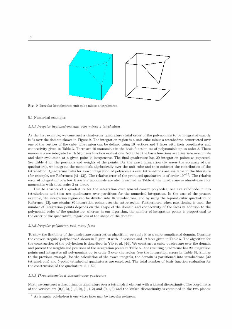
Fig. 9 Irregular heptahedron: unit cube minus a tetrahedron.

5.1 Numerical examples

5.1.1 Irregular heptahedron: unit cube minus a tetrahedron

As the first example, we construct a third-order quadrature (total order of the polynomials to be integrated exactly

is 3) over the domain shown in Figure 9. The integration region is a unit cube minus a tetrahedron constructed over

one of the vertices of the cube. The region can be defined using 10 vertices and 7 faces with their coordinates and

connectivity given in Table 3. There are 20 monomials in the basis function set of polynomials up to order 3. These

monomials are integrated with 576 basis function evaluations. Note that the basis functions are trivariate monomials

and their evaluation at a given point is inexpensive. The final quadrature has 20 integration points as expected.

See Table 4 for the positions and weights of the points. For the exact integration (to assess the accuracy of our

quadrature), we integrate the monomials algebraically over the unit cube and then subtract the contribution of the

tetrahedron. Quadrature rules for exact integration of polynomials over tetrahedrons are available in the literature

(for example, see References [41–43]). The relative error of the produced quadrature is of order 10−15. The relative

error of integration of a few trivariate monomials are also presented in Table 4: the quadrature is almost-exact for

monomials with total order 3 or lower.

Due to absence of a quadrature for the integration over general convex polyhedra, one can subdivide it into

tetrahedrons and then use quadratures over partitions for the numerical integration. In the case of the present

example, the integration region can be divided into 16 tetrahedrons, and by using the 5-point cubic quadrature of

Reference [42], one obtains 80 integration points over the entire region. Furthermore, when partitioning is used, the

number of integration points depends on the shape of the domain and connectivity of the faces in addition to the

polynomial order of the quadrature, whereas in our algorithm, the number of integration points is proportional to

the order of the quadrature, regardless of the shape of the domain.

5.1.2 Irregular polyhedron with many faces

To show the flexibility of the quadrature construction algorithm, we apply it to a more complicated domain. Consider

the convex irregular polyhedron2 shown in Figure 10 with 18 vertices and 19 faces given in Table 5. The algorithm for

the construction of the polyhedron is described in Yip et al. [44]. We construct a cubic quadrature over the domain

and present the weights and positions of the integration points in Table 6—the resulting quadrature has 20 integration

points and integrates all polynomials up to order 3 over the region (see the integration errors in Table 6). Similar

to the previous example, for the calculation of the exact integrals, the domain is partitioned into tetrahedrons (32

tetrahedrons) and 5-point tetrahedral quadratures are employed. The total number of basis function evaluation for

the construction of the quadrature is 1152.

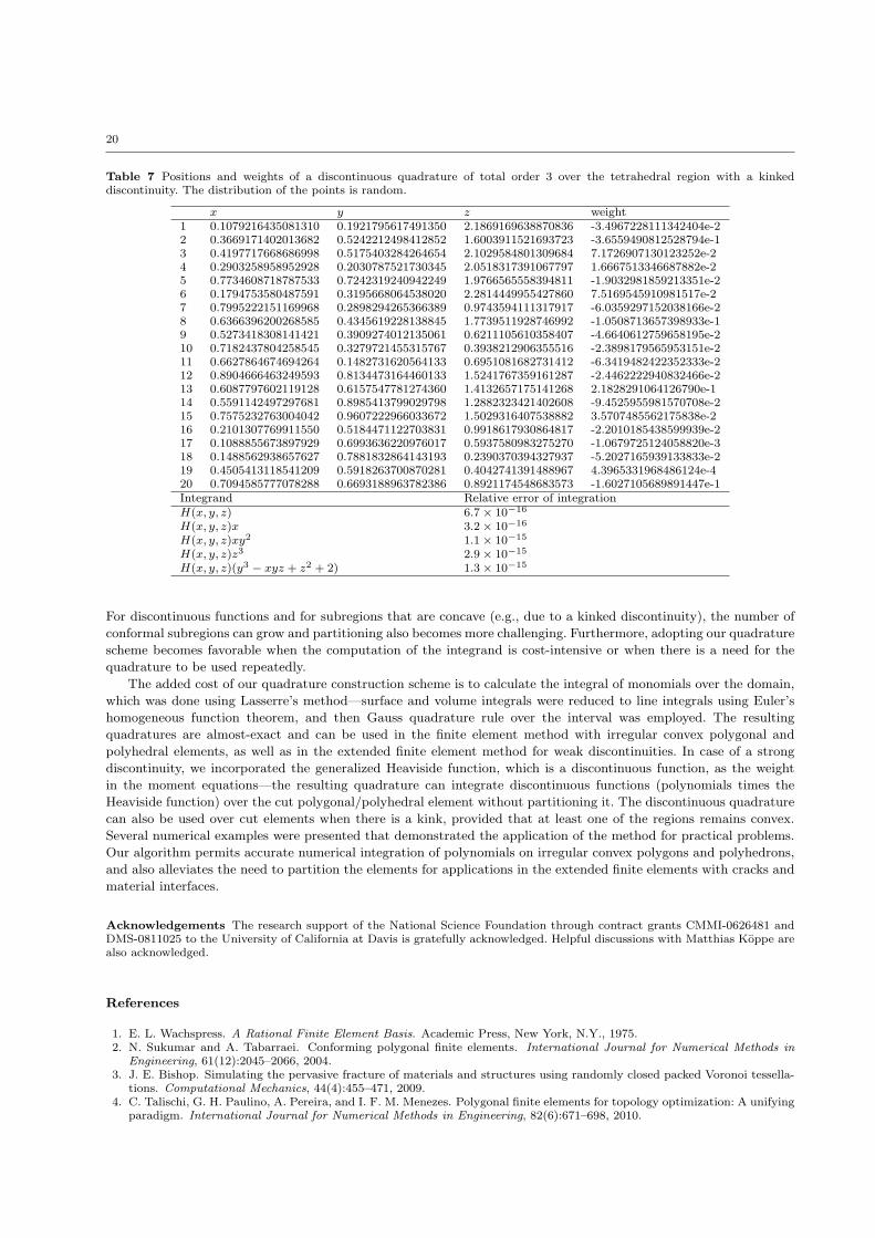
5.1.3 Three-dimensional discontinuous quadrature

Next, we construct a discontinuous quadrature over a tetrahedral element with a kinked discontinuity. The coordinates

of the vertices are (0, 0, 3), (1, 0, 0), (1, 1, 2) and (0, 1, 0) and the kinked discontinuity is contained in the two planes:

2 An irregular polyhedron is one whose faces may be irregular polygons.

17

Table 3 Coordinates of the vertices and connectivity of the faces of the irregular heptahedron.

Vertices x y z1 1 0 02 1 1 03 0 1 04 0 0 05 1 0 16 1 1/2 17 1 1 1/28 1/2 1 19 0 1 110 0 0 1Faces Connectivity1 1, 2, 7, 6, 52 2, 3, 9, 8, 73 3, 4, 10, 94 5, 10, 4, 15 1, 4, 3, 26 5, 6, 8, 9, 107 6, 7, 8

Table 4 Positions and weights of a quadrature of total order 3 over the irregular heptahedron. The distribution of the pointsis random.

x y z weight1 0.6319856330992721 0.3524980414890462 0.5412161514545703 -0.99351655500120632 0.6112764603706613 0.2842460438220646 0.3456663600269569 0.40334119130318563 0.7476367049213167 0.3048071046880173 0.3881636404073822 0.34860490596535234 0.3648365197758032 0.6166082077388840 0.2553757324215449 0.66613291639807305 0.5074440285205465 0.7460607627741637 0.3985478210006686 -0.03690304872471236 0.4765105250092727 0.7079144951920009 0.3014705556484012 -0.15030125119532317 0.4104124440063532 0.4843159604043282 0.3126199335638323 -0.51589776684119028 0.2692967426831230 0.3394285421344097 0.3704014498867298 0.30707822263040069 0.6741626711862849 0.2655279045109828 0.6247633334584989 -0.031760446938727010 0.5278539603101956 0.5783627395311751 0.5223108126435833 -1.325237475306321911 0.6571567227924915 0.5223598802072030 0.7874698497496101 0.238006272770098512 0.7744535851182366 0.4747523895799468 0.6538825745568189 0.334061804826052613 0.7698639943845597 0.6625050391811230 0.3944470991755144 0.020938309081937514 0.6857658120815648 0.7421898806441541 0.4698496012443164 1.023928969308099115 0.8413216125986441 0.7701327382165640 0.5201915416006866 -0.284131034746577116 0.5248245683630873 0.6774033818011266 0.7610592011515803 -0.251020275028244817 0.3089164830432281 0.6565782869258732 0.7789157096197711 0.577987568528084518 0.4818905673003364 0.4508105701035444 0.6867311245003529 0.923843813585114319 0.3906034486580987 0.4372177475524537 0.8125540888317655 -0.886089902873606720 0.4253557947192131 0.2923358620856172 0.7756170122266641 0.6101004489261785Integrand Relative error of integration1 5.6 × 10−16

x 6.9 × 10−16

xy2 1.8 × 10−16

z3 5.8 × 10−16

y3 − xyz + z2 + 2 7.4 × 10−16

z = 2.1 and y + z = 2.6 (see Figure 11 for the geometry of the domain and configuration of the discontinuity). To

the best of the authors’ knowledge no such quadrature is available in the literature due to the complexity of the

domain of integration, and the only way to integrate the discontinuous functions over the domain is by splitting

it into partitions over which quadratures are available. Knowing that the whole element (tetrahedron) and at least

one of the divisions are convex, one can use our algorithm to integrate the basis functions. We use the generalized

Heaviside function as the weight of the quadrature, which is equal to +1 in the top part and −1 in the bottom part. A

cubic-order quadrature with 20 integration points is constructed over the prescribed cut element (see (14) and (16) for

the construction and application of the quadrature). The positions and weights of the discontinuous quadrature and

the error of integration for a few functions are given in Table 7. The relative norm of the quadrature error is of order

10−15. The exact integration, for assessing the accuracy of the constructed quadrature, is performed using (17): the

top division is prescribed in terms of the tetrahedron minus the bottom division which is partitioned into tetrahedrons

18

Fig. 10 Convex polyhedron with 18 vertices and 19 faces.

Table 5 Coordinates of the vertices and connectivity of the faces of the convex polyhedron.

Vertices x y z1 2.956100000000000 3.293900000000000 5.0000000000000002 2.998750000000000 5.000000000000000 3.2512500000000003 2.998750000000000 5.000000000000000 6.7487500000000004 3.043590000000000 6.793590000000000 5.0000000000000005 3.247500000000000 3.002500000000000 5.0000000000000006 5.000000000000000 5.000000000000000 1.2500000000000007 5.000000000000000 3.094740000000000 3.1552600000000008 5.000000000000000 3.094740000000000 6.8447400000000009 5.000000000000000 5.000000000000000 8.75000000000000010 3.530000000000000 7.280000000000000 5.00000000000000011 5.000000000000000 6.912500000000000 3.16250000000000012 5.000000000000000 6.912500000000000 6.83750000000000013 6.843040000000000 3.191740000000000 4.90130000000000014 6.843040000000000 3.191740000000000 5.09870000000000015 6.541670000000000 5.000000000000000 7.20833000000000016 6.276090000000000 6.593480000000000 5.88043000000000017 6.276090000000000 6.593480000000000 4.11957000000000018 6.541670000000000 5.000000000000000 2.791670000000000Faces Connectivity1 2, 1, 32 5, 1, 2, 6, 73 5, 8, 9, 3, 14 10, 4, 2, 6, 115 10, 4, 3, 9, 126 5, 7, 137 9, 15, 14, 88 9, 15, 16, 129 10, 12, 1610 6, 7, 13, 1811 6, 18, 17, 1112 15, 16, 17, 1813 2, 3, 414 5, 13, 1415 5, 14, 816 10, 16, 1717 10, 17, 1118 15, 18, 1319 15, 13, 14

19

Table 6 Positions and weights of a quadrature of total order 3 over the convex polyhedron. The distribution of the points israndom.

x y z weight1 4.065709795565736 4.162155997653544 4.727895668889981 -4.4592942213264402 3.945006242841623 4.296614254864239 5.032658948186411 22.872080053302763 3.956317838457130 5.072225279458875 4.081156810615234 -0.8900070975660544 4.020727362544046 5.152664082058308 5.790992552942226 -10.613922429727035 3.929908521745204 6.037653413585427 5.161937640050013 15.221653576491556 4.984059196662368 5.146949262353924 3.188314234217299 34.123311544565837 5.000688428115388 4.819017447794130 3.565541876877864 -33.997824585903538 5.075009194166556 4.144397175475000 3.845760521061140 13.359347478695319 5.094651222398438 4.007924304779445 5.708146462338654 -13.1899933123627510 4.867348506541593 3.834165799201663 6.297954735625012 5.29127905346387211 4.894822158847349 4.820980719998183 6.499507455597497 -20.2767619019626112 4.890851876647310 4.819388016389012 6.879695758948051 26.4144147216608713 4.881218611500460 5.932051595186250 4.213149790015777 -11.8427690405773814 4.848351922830217 5.963614996717538 5.844249251200039 2.45856642798197915 5.828300751817223 4.115615418801242 4.963750462040973 17.6357804064810416 5.924660436836890 5.112274393992814 6.296378681170026 -0.58204920421203317 5.653195583059173 5.886988405049809 5.618342631081721 3.17744466375551618 5.558007746733869 5.604394796117942 4.702997087185103 8.89689788857949119 5.660217464475206 5.919982983444119 4.482252027916771 8.09191441858531620 5.715307400851893 4.972397189965120 4.082262791570251 -10.58932553713920Integrand Relative error of integration1 7.3 × 10−14

x 1.3 × 10−15

xy2 4.2 × 10−16

z3 7.0 × 10−16

y3 − xyz + z2 + 2 2.9 × 10−15

(a) (b) (c)Fig. 11 A tetrahedron with a kinked discontinuity. (a) the geometry of the tetrahedron; and (b) and (c) configuration of thekinked discontinuity with a faceted plot and a wire plot, respectively.

for the sake of integration, and a 5-point quadrature over the tetrahedrons is used (13 tetrahedrons). The number of

basis function evaluations for the quadrature construction is 576.

6 Concluding remarks

We presented a technique for the integration of polynomials over irregular convex polygons and polyhedrons. While

the position of the quadrature points were predetermined, moment equations were solved in order to obtain the

corresponding weights. We chose the number of integration points to be greater than the number of equations, and

then solved the moment equations in a least-squares sense to obtain the sparsest solution. With this technique,

one has the freedom to select the integration points at desired locations. The number of integration points in the

produced quadrature is proportional to the polynomial order of the quadrature, and is not affected by the geometry

of the integration domain. In contrast to our approach, the number of integration points in the quadratures obtained

through partitioning of the domain depends on the shape of the polytope in addition to the polynomial degree.

20

Table 7 Positions and weights of a discontinuous quadrature of total order 3 over the tetrahedral region with a kinkeddiscontinuity. The distribution of the points is random.

x y z weight1 0.1079216435081310 0.1921795617491350 2.1869169638870836 -3.4967228111342404e-22 0.3669171402013682 0.5242212498412852 1.6003911521693723 -3.6559490812528794e-13 0.4197717668686998 0.5175403284264654 2.1029584801309684 7.1726907130123252e-24 0.2903258958952928 0.2030787521730345 2.0518317391067797 1.6667513346687882e-25 0.7734608718787533 0.7242319240942249 1.9766565558394811 -1.9032981859213351e-26 0.1794753580487591 0.3195668064538020 2.2814449955427860 7.5169545910981517e-27 0.7995222151169968 0.2898294265366389 0.9743594111317917 -6.0359297152038166e-28 0.6366396200268585 0.4345619228138845 1.7739511928746992 -1.0508713657398933e-19 0.5273418308141421 0.3909274012135061 0.6211105610358407 -4.6640612759658195e-210 0.7182437804258545 0.3279721455315767 0.3938212906355516 -2.3898179565953151e-211 0.6627864674694264 0.1482731620564133 0.6951081682731412 -6.3419482422352333e-212 0.8904666463249593 0.8134473164460133 1.5241767359161287 -2.4462222940832466e-213 0.6087797602119128 0.6157547781274360 1.4132657175141268 2.1828291064126790e-114 0.5591142497297681 0.8985413799029798 1.2882323421402608 -9.4525955981570708e-215 0.7575232763004042 0.9607222966033672 1.5029316407538882 3.5707485562175838e-216 0.2101307769911550 0.5184471122703831 0.9918617930864817 -2.2010185438599939e-217 0.1088855673897929 0.6993636220976017 0.5937580983275270 -1.0679725124058820e-318 0.1488562938657627 0.7881832864143193 0.2390370394327937 -5.2027165939133833e-219 0.4505413118541209 0.5918263700870281 0.4042741391488967 4.3965331968486124e-420 0.7094585777078288 0.6693188963782386 0.8921174548683573 -1.6027105689891447e-1Integrand Relative error of integrationH(x, y, z) 6.7 × 10−16

H(x, y, z)x 3.2 × 10−16

H(x, y, z)xy2 1.1 × 10−15

H(x, y, z)z3 2.9 × 10−15

H(x, y, z)(y3 − xyz + z2 + 2) 1.3 × 10−15

For discontinuous functions and for subregions that are concave (e.g., due to a kinked discontinuity), the number of

conformal subregions can grow and partitioning also becomes more challenging. Furthermore, adopting our quadrature

scheme becomes favorable when the computation of the integrand is cost-intensive or when there is a need for the

quadrature to be used repeatedly.

The added cost of our quadrature construction scheme is to calculate the integral of monomials over the domain,

which was done using Lasserre’s method—surface and volume integrals were reduced to line integrals using Euler’s

homogeneous function theorem, and then Gauss quadrature rule over the interval was employed. The resulting

quadratures are almost-exact and can be used in the finite element method with irregular convex polygonal and

polyhedral elements, as well as in the extended finite element method for weak discontinuities. In case of a strong

discontinuity, we incorporated the generalized Heaviside function, which is a discontinuous function, as the weight

in the moment equations—the resulting quadrature can integrate discontinuous functions (polynomials times the

Heaviside function) over the cut polygonal/polyhedral element without partitioning it. The discontinuous quadrature

can also be used over cut elements when there is a kink, provided that at least one of the regions remains convex.

Several numerical examples were presented that demonstrated the application of the method for practical problems.

Our algorithm permits accurate numerical integration of polynomials on irregular convex polygons and polyhedrons,

and also alleviates the need to partition the elements for applications in the extended finite elements with cracks and

material interfaces.

Acknowledgements The research support of the National Science Foundation through contract grants CMMI-0626481 andDMS-0811025 to the University of California at Davis is gratefully acknowledged. Helpful discussions with Matthias Koppe arealso acknowledged.

References

1. E. L. Wachspress. A Rational Finite Element Basis. Academic Press, New York, N.Y., 1975.2. N. Sukumar and A. Tabarraei. Conforming polygonal finite elements. International Journal for Numerical Methods in

Engineering, 61(12):2045–2066, 2004.3. J. E. Bishop. Simulating the pervasive fracture of materials and structures using randomly closed packed Voronoi tessella-

tions. Computational Mechanics, 44(4):455–471, 2009.4. C. Talischi, G. H. Paulino, A. Pereira, and I. F. M. Menezes. Polygonal finite elements for topology optimization: A unifying

paradigm. International Journal for Numerical Methods in Engineering, 82(6):671–698, 2010.

21

5. M. Wicke, M. Botsch, and M. Gross. A finite element method on convex polyhedra. Computer Graphics Forum, 26(3):355–364, 2007.

6. S. Martin, P. Kaufmann, M. Botsch, M. Wicke, and M. Gross. Polyhedral finite elements using harmonic basis functions.Computer graphics forum, 27(5):1521–1529, 2008.

7. P. Milbradt and T. Pick. Polytope finite elements. International Journal for Numerical Methods in Engineering, 73:1811–1835, 2008.

8. M. M. Rashid and P. M. Gullett. On a finite element method with variable element topology. Computer Methods in AppliedMechanics and Engineering, 190(11–12):1509–1527, 2000.

9. M. M. Rashid and M. Selimotic. A three-dimensional finite element method with arbitrary polyhedral elements. Interna-tional Journal for Numerical Methods in Engineering, 67:226–252, 2006.

10. P. Kaufmann, S. Martin, M. Botsch, and M. Gross. Flexible simulation of deformable models using discontinuous GalerkinFEM. Graphical Models, 71(4):153–167, 2009. Special Issue of ACM SIGGRAPH/Eurographics Symposium on ComputerAnimation 2008.

11. T. V. Voitovich and S. Vandewalle. Exact integration formulas for the finite volume element method on simplicial meshes.Numerical Methods for Partial Differential Equations, 23(5):1059–1082, 2007.

12. F. Brezzi, K. Lipnikov, and V. Simoncini. A family of mimetic finite difference methods on polygonal and polyhedralmeshes. Mathematical Models and Methods in Applied Sciences, 15(10):1533–1551, 2005.

13. L. B. da Veiga, V. Gyrya, K. Lipnikov, and G. Manzini. Mimetic finite difference method for the Stokes problem onpolygonal meshes. Journal of Computational Physics, 228:7215–7232, 2009.

14. L. B. da Veiga, K. Lipnikov, and G. Manzini. Error analysis for a mimetic discretization of the steady Stokes problem onpolyhedral meshes. SIAM Journal on Numerical Analysis, 48(4):1419–1443, 2010.

15. N. Moes, J. Dolbow, and T. Belytschko. A finite element method for crack growth without remeshing. International Journalfor Numerical Methods in Engineering, 46(1):131–150, 1999.

16. N. Sukumar, D. L. Chopp, N. Moes, and T. Belytschko. Modeling holes and inclusions by level sets in the extendedfinite-element method. Computer Methods in Applied Mechanics and Engineering, 190(46–47):6183–6200, 2001.

17. J. B. Lasserre. Integration on a convex polytope. Proceedings of the American Mathematical Society, 126(8):2433–2441,1998.

18. J. B. Lasserre. Integration and homogeneous functions. Proceedings of the American Mathematical Society, 127(3):813–818,1999.

19. V. Baldoni, N. Berline, J. A. De Loera, M. Koppe, and M. Vergne. How to integrate a polynomial over a simplex.Mathematics of Computation, 2010. DOI: 10.1090/S0025-5718-2010-02378-6.

20. P. C. Hammer, O. J. Marlowe, and A. H. Stroud. Numerical integration over simplexes and cones. Mathematical Tablesand Other Aids to Computation, 10:130–137, 1956.

21. Y. Liu and M. Vinokur. Exact integrations of polynomials and symmetric quadrature formulas over arbitrary polyhedralgrids. Journal of Computational Physics, 140:122–147, 1998.

22. J. B. Lasserre and K. E. Avrachenkov. The multi-dimensional version ofR b

a xpdx. The American Mathematical Monthly,108(2):151–154, 2001.

23. H. G. Timmer and J. M. Stern. Computation of global geometric properties of solid objects. Computer Aided Design,12(6):301–304, 1980.

24. C. Cattani and A. Paoluzzi. Boundary integration over linear polyhedra. Computer Aided Design, 22(2):130–135, 1990.25. F. Bernardini. Integration of polynomials over n-dimensional polyhedra. Computer Aided Design, 23(1):51–58, 1991.26. B. Mirtich. Fast and accurate computation of polyhedral mass properties. Journal of Graphics, GPU, and Game Tools,

1(2):31–50, 1996.27. H. T. Rathod and H. S. Govinda Rao. Integration of polynomials over n-dimensional linear polyhedra. Computers and

Structures, 65(6):829–847, 1997.28. G. Dasgupta. Integration within polygonal finite elements. Journal of Aerospace Engineering, 16(1):9–18, 2003.29. S. E. Mousavi, H. Xiao, and N. Sukumar. Generalized Gaussian quadrature rules on arbitrary polygons. International

Journal for Numerical Methods in Engineering, 82(1):99–113, 2010.30. H. Xiao and Z. Gimbutas. A numerical algorithm for the construction of efficient quadratures in two and higher dimensions.

Computers and Mathematics with Applications, 59:663–676, 2010.31. S. E. Mousavi and N. Sukumar. Generalized Duffy transformation for integrating vertex singularities. Computational

Mechanics, 45(2–3):127–140, 2010.32. S. E. Mousavi and N. Sukumar. Generalized Gaussian quadrature rules for discontinuities and crack singularities in the

extended finite element method. Computer Methods in Applied Mechanics and Engineering, 199(49–52):3237–3249, 2010.33. J. N. Lyness and D. Jespersen. Moderate degree symmetric quadrature rules for the triangle. Journal of the Institute of

Mathematics and its Applications, 15:19–32, 1975.34. J. N. Lyness and G. Monegato. Quadrature rules for regions having regular hexagonal symmetry. SIAM Journal on

Numerical Analysis, 14(2):283–295, 1977.35. D. A. Dunavant. High degree efficient symmetrical Gaussian quadrature rules for the triangle. International Journal for

Numerical Methods in Engineering, 21:1129–1148, 1985.36. S. Wandzura and H. Xiao. Symmetric quadrature rules on a triangle. Computers and Mathematics with Applications,

45:1829–1840, 2003.37. G. Ventura. On the elimination of quadrature subcells for discontinuous functions in the eXtended Finite-Element Method.

International Journal for Numerical Methods in Engineering, 66:761–795, 2006.38. D. J. Holdych, D. R. Noble, and R. B. Secor. Quadrature rules for triangular and tetrahedral elements with generalized

functions. International Journal for Numerical Methods in Engineering, 73:1310–1327, 2008.39. S. Natarajan, D. R. Mahapatra, and S. P. A. Bordas. Integrating strong and weak discontinuities without integration subcells

and example applications in an XFEM/GFEM framework. International Journal for Numerical Methods in Engineering,83:269–294, 2010.

40. K. W. Cheng and T. P. Fries. Higher-order XFEM for curved strong and weak discontinuities. International Journal forNumerical Methods in Engineering, 82:564–590, 2010.

22

41. P. Silvester. Symmetric quadrature formulae for simplexes. Mathematics of Computation, 24(109):95–100, 1970.42. K. S. Sunder and R. A. Cookson. Integration points for triangles and tetrahedrons obtained from the Gaussian quadrature

points for a line. Computers and Structures, 21(5):881–885, 1985.43. P. Keast. Moderate-degree tetrahedral quadrature formulas. Computer Methods in Applied Mechanics and Engineering,

55:339–348, 1986.44. M. Yip, J. Mohle, and J. E. Bolander. Automated modeling of three-dimensional structural components using irregular

lattices. Computer-Aided Civil and Infrastructure Engineering, 20:393–407, 2005.