Numerical investigation and evaluation of optimum hydrodynamic performance of ahorizontal axis hydrokinetic turbineSuchi Subhra Mukherji, Nitin Kolekar, Arindam Banerjee, and Rajiv Mishra Citation: Journal of Renewable and Sustainable Energy 3, 063105 (2011); doi: 10.1063/1.3662100 View online: http://dx.doi.org/10.1063/1.3662100 View Table of Contents: http://scitation.aip.org/content/aip/journal/jrse/3/6?ver=pdfcov Published by the AIP Publishing Articles you may be interested in Aerodynamic performance and characteristic of vortex structures for Darrieus wind turbine. II. The relationshipbetween vortex structure and aerodynamic performance J. Renewable Sustainable Energy 6, 043135 (2014); 10.1063/1.4893776 Three-dimensional numerical analysis on blade response of a vertical-axis tidal current turbine under operationalconditions J. Renewable Sustainable Energy 6, 043123 (2014); 10.1063/1.4892952 A coupled hydro-structural design optimization for hydrokinetic turbines J. Renewable Sustainable Energy 5, 053146 (2013); 10.1063/1.4826882 Numerical study on aerodynamic performances of the wind turbine rotor with leading-edge rotation J. Renewable Sustainable Energy 4, 063103 (2012); 10.1063/1.4765697 Dynamic stall analysis of horizontal-axis-wind-turbine blades using computational fluid dynamics AIP Conf. Proc. 1440, 953 (2012); 10.1063/1.4704309

This article is copyrighted as indicated in the article. Reuse of AIP content is subject to the terms at: http://scitation.aip.org/termsconditions. Downloaded to IP:

128.180.11.213 On: Tue, 12 May 2015 19:56:15

Numerical investigation and evaluation of optimumhydrodynamic performance of a horizontal axishydrokinetic turbine

Suchi Subhra Mukherji,1 Nitin Kolekar,1 Arindam Banerjee,1,a)

and Rajiv Mishra2

1Department of Mechanical and Aerospace Engineering, Missouri University of Scienceand Technology, Rolla, Missouri 65409, USA2Department of Materials Science and Engineering, University of North Texas, Denton,Texas 76203, USA

(Received 16 February 2011; accepted 28 October 2011; published online 21 November2011)

The hydrodynamic performance of horizontal axis hydrokinetic turbines (HAHkTs)

under different turbine geometries and flow conditions is discussed. Hydrokinetic

turbines are a class of zero-head hydropower systems which utilize kinetic energy of

flowing water to drive a generator. However, such turbines very often suffer from

low-efficiency which is primarily due to its operation in a low tip-speed ratio (�4)

regime. This makes the design of a HAHkT a challenging task. A detailed computa-

tional fluid dynamics study was performed using the k-x shear stress transport turbu-

lence model to examine the effect of various parameters like tip-speed ratio, solidity,

angle of attack, and number of blades on the performance HAHkTs having power

capacities of �12 kW. For this purpose, a three-dimensional numerical model was

developed and validated with experimental data. The numerical studies estimate opti-

mum turbine solidity and blade numbers that produce maximum power coefficient at

a given tip speed ratio. Simulations were also performed to observe the axial velocity

ratios at the turbine rotor downstream for different tip speed ratios which provide

quantitative details of energy loss suffered by each turbine at an ambient flow condi-

tion. The velocity distribution provides confirmation of the stall-delay phenomenon

due to the effect of rotation of the turbine and a further verification of optimum tip

speed ratio corresponding to maximum power coefficient obtained from the solidity

analysis. VC 2011 American Institute of Physics. [doi:10.1063/1.3662100]

I. INTRODUCTION

Conventional hydropower has been considered as a sustainable energy resource for several

decades and presently supplies almost 100 GW of energy annually, which accounts for almost

10% of U.S. total energy requirement.1 However, due to site availability constraints and envi-

ronmental impact of the dams and reservoirs in the available rivers, it is projected that conven-

tional hydropower systems will be unable to meet the 14% rise in total energy demand until the

year 2035.2 The entire mid-west region of USA has more than 6000 miles of river banks, a sig-

nificant portion of which being fed by low depth rivers and remains untapped for power genera-

tion. This presents an urgent need of a low-head hydropower system that can extract power

from low depth rivers to meet the increasing energy requirement. Power from moving water-

flow provides such form of hydropower systems where turbines submerged in rivers (hydroki-

netic turbines) or tides/oceans (marine current turbines (MCTs)) offer an exciting proposition of

utilizing kinetic energy of flowing water to drive a generator without diverting the flow path.3–5

a)Author to whom correspondence should be addressed. Electronic mail: banerjeea@mst.edu. Tel.: 573-341-4494. FAX:

573-341-4607.

1941-7012/2011/3(6)/063105/18/$30.00 VC 2011 American Institute of Physics3, 063105-1

JOURNAL OF RENEWABLE AND SUSTAINABLE ENERGY 3, 063105 (2011)

This article is copyrighted as indicated in the article. Reuse of AIP content is subject to the terms at: http://scitation.aip.org/termsconditions. Downloaded to IP:

128.180.11.213 On: Tue, 12 May 2015 19:56:15

As a result, the system provides flexibility of its usage from conventional hydropower systems

where the potential energy of the water was being utilized by constructing dams/reservoirs to

generate electricity.

The principle of operation behind hydrokinetic turbines is similar to that of wind turbines

in principle; however, since the density of water is 850 times greater than air, hydrokinetic tur-

bines allow for increased energy extraction from a given flow stream. In addition, the flow

regimes at which hydrokinetic turbines operate are different to conventional wind turbines. The

unidirectional nature of river flow eliminates expensive yawing mechanism for hydrokinetic tur-

bines making it cost effective and structurally simpler. Moreover, hydrokinetic technologies do

not require large infrastructure such as dams and powerhouses, which results in significantly

faster deployment time and reduced manufacturing and operating costs.6,7 Another advantage of

hydrokinetic turbines is their modular nature which leads to a scalable energy output and con-

tinuous energy production under zero static head. These attributes reduce the need of energy

storage capacity, and as a result of this, hydrokinetic turbines find increased usage in remote

locations.3,5 However, the primary barrier to commercialization of this technology lies in its

low efficiency8 which is primarily due to its operation in a low tip-speed ratio (TSR)� 4 re-

gime. This makes the design of hydrokinetic turbines a challenging task. Since an efficient and

cost-effective energy production is directly related to the proper selection of design parameters,

an optimum turbine design is required for effective use under variable flow conditions.

Just as in conventional hydraulic turbines, hydrokinetic turbines are primarily classified

based upon the orientation of turbine rotor relative to the primary flow direction. Two types of

hydrokinetic turbines are possible depending on their principle of operation: horizontal axis tur-

bine where the axis of rotation is parallel to the primary flow direction9,10 and vertical axis or

cross-flow turbine where the rotational axis is perpendicular to the incoming water.2,11 The cur-

rent work focuses on horizontal axis hydrokinetic turbines, henceforth referred to as HAHkTs,

due to its relatively higher efficiency, lower incidence losses, less vibration, and more uniform

lift forces than its vertical axis counterpart.5,8,12 As in conventional wind turbines, the blades in

HAHkTs move perpendicular to the fluid motion receiving power over the entire cycle of rota-

tion. In contrast, vertical axis turbines involve various reciprocating actions requiring hydrofoil

surfaces to back-track against the fluid for part of the cycle which is expected to result in lower

efficiency. Thus, the swept area of our HAHkTs always faces the fluid unlike the vertical axis

turbines where the swept area is perpendicular to the direction of flow. As a result, part of the

swept area for vertical axis turbines is simply being blown around at anon-optimal angle that

reduces lift resulting in a lower efficiency than their horizontal counterparts.8 Our design of

HAHkTs is meant for operation in a river stream with a mean speed of �2 m/s which limits

the operation to TSR< 4. A review of available literature on HAWTs (horizontal axis wind tur-

bines) and MCTs reveals that the Cp would be restricted to �0.25 for low TSR.9,13–18

Over the last decade, several experimental and numerical investigations have been reported

on horizontal and vertical/cross-flow water turbines from the perspective of flow dynamics and

the influence of several non-dimensional parameters on the hydrodynamic performance of the

turbines.11 Non-dimensional parameters studied include: Reynolds number (Re) (ratio of inertia

force to viscous force), TSR (ratio of blade tip speed to fluid speed), and solidity (ratio of blade

chord length times the number of blades to turbine circumference). In addition, the number of

blades also plays a critical role in determining the performance of the turbines.2,11 Consul11

investigated the influence of solidity on the increased performance of a cross flow turbine using

two-dimensional numerical simulation. They reported an increase in maximum power coeffi-

cient with an increase in blade number, i.e., greater solidity with entire power curve being

shifted to a lower TSR. Hwang2 performed a two-dimensional numerical study as well as an ex-

perimental study to understand the effects of number of blades, the chord length variation, the

TSR variation, and the shape of the hydrofoil on the overall performance of a cross-flow tur-

bine. They also reported a similar increase in the power coefficient at a lower TSR with

increased rotor solidity. In addition, their experimental results showed good agreement with nu-

merical results with an under-prediction of generated power due to the additional drag forces.

Batten discussed the effects of blade pitch angle and changes in camber on stall performance

063105-2 Mukherji et al. J. Renewable Sustainable Energy 3, 063105 (2011)

This article is copyrighted as indicated in the article. Reuse of AIP content is subject to the terms at: http://scitation.aip.org/termsconditions. Downloaded to IP:

128.180.11.213 On: Tue, 12 May 2015 19:56:15

and delay of cavitation in marine current turbines.9,17 Their analysis, however, is based on high

aspect ratio blades where the flow is nearly two-dimensional and can be modeled using blade

element momentum (BEM) theory. Myers10,19 also performed BEM calculations and an experi-

mental study to determine the power output over a range of flow speeds and blade pitch for

horizontal axis marine turbines. Although their pre-stall power measurements agreed well with

BEM theory, the post-stall measurements were over-predicted due to the failure of the theoreti-

cal model to accurately predict stall-delay under rotational motion. Although not investigated

for HAHkTs, near wake aerodynamics have been studied for wind turbines to understand the

crucial role of wakes on the performance and physical processes of power extraction from the

turbine rotation.13,20,21 However, no extensive study has been reported to date, which discusses

the effect of solidity, angle of attack, blade number, and stall delay on the performance of small

HAHkTs. The current work is limited to low capacity turbines �12 kW primarily due to their

usage in military/naval applications and for civilian usage in rural hard to reach communities.

A detailed numerical investigation for performance evaluation of low capacity HAHkTs is dis-

cussed—the turbines are designed to extract power from an average water depth of 5-10 m.

The optimum operating conditions and geometric characteristics of HAHkTs were deter-

mined for the variables such as TSR, solidity, number of blades, and Re using computational

fluid dynamics (CFD) analysis. The purpose of this study was two-fold: (a) it lays a strong

foundation for designing and testing HAHkTs system of �12 kW capacity with optimum geo-

metric and performance characteristics and (b) provides quantitative details regarding the maxi-

mum amount of power that can be extracted from a given flow condition using such turbines

under a variety of design conditions with and without an optimized blade design—thus embrac-

ing the possibility of having both low (non-optimized) and high cost (optimized) systems that

would appeal to a wide range of consumers. The paper is organized as follows: in Sec. II, the

mathematical and numerical models associated with hydrodynamic performance of HAHkTs

are discussed. Section II also provides detailed information regarding the computational geome-

try used in this work with primary focus on grid and domain specification, boundary conditions,

and the solution discretization methodology. Section III discuss the results obtained from three

dimensional numerical simulations. The numerical model was first validated with existing ex-

perimental results (in air) followed by a further analysis considering individual effect of the

variables discussed above. In conclusion, Sec. IV analyses our findings from the numerical

model and provides the implication of turbine TSR, solidity, number of blades, and Re on the

optimum turbine performance under given operating conditions.

II. NUMERICAL METHODOLOGY

A. Governing equations

The numerical modeling of HAHkTs is complicated due to the rotation of the turbine

coupled with turbulence and stall effects. A moving reference frame was incorporated to take

this into account and transform an unsteady flow in an inertial (stationary) frame to a steady

flow in a non-inertial (moving) frame. A constant rotational speed (X) is provided on a steadily

rotating flow geometry, and equations of fluid motion have been transformed to a rotating frame

as shown below,22

r � ~Ur ¼ 0; (1)

q@

@tð~UrÞ þ r � ð~Ur

~UrÞ þ ð2~X� ~Ur þ ~X� ~X�~rÞ� �

¼ �rpþr � sr; (2)

where ~Ur is the relative velocity viewed from rotating reference frame, X is the rotational speed

of the turbine, qð2~X� ~UrÞ is the Coriolis force, qð~X� ~X� rÞ is the centrifugal force, and rpis the pressure gradient across the turbine. The viscous stress tensor (sr) is defined as

063105-3 Performance of hydrokinetic turbines J. Renewable Sustainable Energy 3, 063105 (2011)

This article is copyrighted as indicated in the article. Reuse of AIP content is subject to the terms at: http://scitation.aip.org/termsconditions. Downloaded to IP:

128.180.11.213 On: Tue, 12 May 2015 19:56:15

sr ¼ leff ½ðr~U þr~UTÞ � 2

3r � ~UI�; (3)

where U is the absolute fluid velocity and I is the identity tensor. The molecular viscosity

(leff) is the sum of the dynamic viscosity (l) and the turbulent eddy viscosity (lt); lt being

calculated from a representative turbulence model. Amongst different turbulence models that

exist in literature, the k-x shear stress transport (SST) model was chosen for the analysis due

to its capability of providing accurate flow-field predictions under adverse pressure gradient

and separated flow conditions both of which are prevalent in HAHkTs.13,23–27 The k-x SST

model is based on the robust and accurate combination, which uses k-x model in near wall

region28 and k-e model in far field region.23,25,29 For flows having adverse pressure gradients,

the level of eddy viscosity primarily determines the accuracy of the turbulence model in pre-

dicting flow separation. Since the standard k-x model fails to predict pressure induced separa-

tion, the model was reconstructed enforcing Bradshaw’s observation in which turbulent shear

stress is proportional to the turbulent kinetic energy in the wake region of the boundary

layer.23 Therefore, using the k-x formulation, the model solves for the transport of turbulent

shear stress which controls the level of eddy viscosity in the outer part of boundary layer.

However, since the k-x model has strong sensitivity to the free-stream value outside the

boundary layer, a transformed k-e model is applied on the far wall region due to its insensi-

tive nature to free stream turbulence.23,24 The governing equations for k-x SST model is

given by

@

@tðqkÞ þ r � ðqk~UÞ ¼ sijr~U � b�qxk þr � ðlþ rkltÞrk½ �; (4)

@

@tðqxÞ þ r � ðqx~UÞ ¼ c

�tsijr~U � bqx2 þr � ðlþ rxltÞrx½ � þ 2ð1� F1Þqrx2

1

xrkrx;

(5)

where F1 denotes the blending function which is designed in such a manner that it assumes the

value of unity inside the viscous sub-layer where original k-x model is activated and it gradu-

ally switches to zero in the wake region where transformed k-e model is activated. The model

constants are the same as provided in the original work23 and are not repeated for the purpose

of brevity.

B. Computational detail and flow domain generation

The present study assumes steady, incompressible flow where the numerical solution is

carried out by solving conservation equations for mass and momentum by deploying an

unstructured grid finite volume methodology using commercial CFD software (Fluent 12.1).

The geometrical model was created using Solidworks and meshed in Ansys Workbench. Nu-

merical simulations were performed to obtain flow hydrodynamics for three-dimensional

rotating boundary conditions. The choice of hydrofoil for HAHkTs is primarily governed by

the geometry that produces maximum lift coefficient (CL) under the operating range of Re.

Previous studies30–32 used SG-6043 airfoil for the design of small wind turbines due to its

capability of producing large CL in the Re range of 105–106. Since the Re for our case also

lies within this range, the SG-6043 airfoil was selected as a hydrofoil for the HAHkT blades.

SG-6043 hydrofoil is a part of a family of untwisted, constant pitch blades. A turbine of ra-

dius (R)¼ 1 m was chosen for the three-dimensional rotational analysis. The computational

domain consists of two cylinders; the inner cylinder extending 10 rotor diameters and the

outer one extending 11 rotor diameters, respectively, in the axial direction (see Fig. 1(a)).

The turbine is placed inside the inner cylinder as shown in Fig. 1(b). Multiple reference

frames have been adapted with a stationary outer cylinder and rotating inner cylinder and an

interior boundary between the two. It is a steady state approximation where the flow in each

moving cell zone is solved using the moving reference frame equations (see Sec. II A). At

063105-4 Mukherji et al. J. Renewable Sustainable Energy 3, 063105 (2011)

This article is copyrighted as indicated in the article. Reuse of AIP content is subject to the terms at: http://scitation.aip.org/termsconditions. Downloaded to IP:

128.180.11.213 On: Tue, 12 May 2015 19:56:15

the interface between the two cell zones, a local reference frame transformation is performed

to enable flow variables in the one zone to be used to calculate the fluxes at the boundary of

the adjacent zone. Since the boundary between the two zones is conformal, i.e., mesh node

locations are identical at the meeting boundary, the interior boundary condition enables

particles to pass through the inner boundary to outer one. Velocity inlet and pressure outlet

boundary conditions are applied with turbulence specifications same as that for the two-

dimensional simulations. A symmetry boundary condition has been provided on the

periphery of the outer cylinder indicating zero normal gradients for all flow variables at the

symmetry plane. The inner and outer cylinder contains approximately 1.2 and 1.15� 106

unstructured tetrahedral/hybrid cells. Grid resolution requirements were well established by

keeping small enough initial normal spacing from the hydrofoil surface yielding yþ

(¼ qusDy/l)� 120, where us is the friction velocity and Dy is the cell size. Though this value

of yþ is large, the blending functions included in the k-x SST model accounted for the

unresolved boundary layers on the blades and no separate wall model was used for the

computations.

The design of the HAHkTs is based on effective water velocities of 1.75–2.25 m/s as

observed in most of the rivers,4 a mean water speed of U1¼ 2 m/s was chosen for the cur-

rent work. The left surface was given velocity inlet boundary conditions with turbulence in-

tensity (I) of 3% and length scale (l) of 0.02 m derived from the empirical relationship based

on the given flow condition: I ¼ 0:16ðReÞ�1=8and l ¼ 0:07L, where L is computed from the

physical dimension of the object, i.e., chord length for the present case. A pressure outlet

boundary condition is provided on the right surface with zero gauge pressure and turbulent

viscosity ratio is set at a value of 10. A second order upwinding discretization schemes have

been employed for all the variables and SIMPLE (Semi-implicit method for pressure linked

equation) algorithm was selected for solving pressure-velocity coupling.33 The PRESTO

(pressure staggering options) scheme has been adopted due to its superiority for flows with

steep pressure gradient such as the present case.34 Convergence criteria have been set such

that the residuals for the continuity, x-momentum, y-momentum, z-momentum, k, and x are

less than 10�4. Details of the simulation variables are listed in Table I. The rotation of the

inner domain adds an additional residual torque to the output torque. In a real-life scenario,

the flowing fluid would cause the blade to rotate and the net torque obtained is converted

into useful power. For our rotating domain simulations, the turbines blades are, however,

subjected to an additional net torque which is a sum of the torque due to the flowing water

and the torque due to the rotating domain. The residual torque due to the rotating domain

was evaluated for each case by running additional simulations with identical rotational

speeds where the free-stream velocity was set to zero. This allowed for evaluating the resid-

ual torque due to the rotating domain from these computations. This residual torque was sub-

tracted from the total torque to calculate the net effective torque on the rotor which was used

FIG. 1. (a) 3D computational domain along with boundary conditions and (b) grid near the rotor hub.

063105-5 Performance of hydrokinetic turbines J. Renewable Sustainable Energy 3, 063105 (2011)

This article is copyrighted as indicated in the article. Reuse of AIP content is subject to the terms at: http://scitation.aip.org/termsconditions. Downloaded to IP:

128.180.11.213 On: Tue, 12 May 2015 19:56:15

for all the power calculations. Table II lists the residual torques for all the cases considered

in this study.

C. Governing parameters

The performance of HAHkTs is primarily determined by the power coefficient (CP) defined as

CP ¼Pout

1

2qU3A

; (6)

where Pout is power output (kW) of the turbine given by the product of torque generated at the

center of the rotor hub and the rotational speed, A is turbine swept area, and U the free-stream

velocity. The thrust coefficient (CT) is defined as

CT ¼T

1

2qU2A

; (7)

where T is the thrust force (N). Turbine TSR is another governing parameter given by

TSR ¼ RXU: (8)

In addition, solidity is related to radius (R), blade chord length (c), and number of blades (N)

as

TABLE I. Parameters for CFD analysis.

Hydrofoil SG-6043

Density (q) 998.2 kg/m3

Pressure (p) 101.3 kPa

Rotor radius (R) 1 m

Chord length (c) 0.15 m, 0.167 m, 0.2 m,

0.25 m, & 0.3 m

Number of blades (N) 2–4

Blade pitch (hP) 10

Rotor speed (X) 3–8 rad/s

Fluid speed (U1) 2 m/s

Turbulence model k-x SST

Interpolating scheme 2nd order upwind

Pressure scheme PRESTO

Residual error 1� 10�4

TABLE II. Residual torque (N-m) and thrust (N) values due to the rotating domain.

N¼ 2 N¼ 3 N¼ 4

TSR Torque Thrust Torque Thrust Torque Thrust

1.5 37.61 248.88 53.05 98.89 58.74 191.84

2.0 65.93 392.59 81.17 185.82 102.83 515.05

2.5 92.85 586.34 119.2 280.25 148.53 344.073

3.0 138.72 751.68 173.19 481.89 233.51 1135.5

3.5 181.43 1146.36 248.92 1165.23 320.21 1525.5

4.0 239.63 1300.54 308.87 1010.43 419.91 1911.03

063105-6 Mukherji et al. J. Renewable Sustainable Energy 3, 063105 (2011)

This article is copyrighted as indicated in the article. Reuse of AIP content is subject to the terms at: http://scitation.aip.org/termsconditions. Downloaded to IP:

128.180.11.213 On: Tue, 12 May 2015 19:56:15

r ¼ Nc

2pR: (9)

In order to validate the numerical results, the basic performance of our HAHkT model was also

evaluated using BEM theory.12 In BEM theory, the rotor blade was divided into a number of

elemental sections, and the torque was calculated from equating the blade forces generated by

these blade elements to the momentum changes occurring in the fluid through the rotor

disc.9,12,17 The formulation of BEM theory was based on the assumptions that there is no

hydrodynamic interaction between the blade elements; forces on the blades are determined by

lift characteristics of the hydrofoil and the drag is zero. The axial induction factor (a) is defined

as the fractional decrease in water speed between the free stream and rotor plane,

a ¼ 1� Ux

U; (10)

where Ux corresponds to axial velocity behind the rotor plane. The angular induction factor (a0)is similarly defined as the fractional increase in angular velocity due to the induced angular ve-

locity at the blades from the conservation of angular momentum. These induction factors a and

a0 are related to the angle of relative water flow (/) by

tan / ¼ 1� a

ð1þ a0Þkr; / ¼ hP þ a; (11)

where kr is the local tip speed ratio at any radial location r from the rotor hub, hP is the turbine

pitch (¼ 10 for present case), and a is the angle of attack. Fig. 2 shows the velocity diagram

for the current configuration. For each turbine blade segment, both a and a0 are determined in

an iterative manner from which CP is calculated by performing numerical integration of the fol-

lowing expression:

CP ¼8

k2

ðk

kh

k3r a0ð1� aÞdkr: (12)

The numerical computations were initially carried out with various levels of refinement of

mesh in order to obtain a grid independent solution. For the present case, the grid independence

study was performed for three dimensional case by calculating the torque generated at the cen-

ter of the rotor hub using eight different grid sizes with total number of cells (Ntotal) varying

between 3.9� 105 and 4.6� 106 (see Fig. 3). The fractional change in the magnitude of the tor-

que was calculated based on the formulation

%Error ¼ T � T0j jT0

� 100; (13)

FIG. 2. Velocity diagram for SG-6043 hydrofoil used in current study.

063105-7 Performance of hydrokinetic turbines J. Renewable Sustainable Energy 3, 063105 (2011)

This article is copyrighted as indicated in the article. Reuse of AIP content is subject to the terms at: http://scitation.aip.org/termsconditions. Downloaded to IP:

128.180.11.213 On: Tue, 12 May 2015 19:56:15

where T denotes torque at different grid sizes and T0 denotes torque correponding to grid inde-

pendent (maximum grid size) geometry. A grid independent solution with a nearly constant

magnitude of torque was observed beyond Ntotal¼ 2.7� 106 where the difference was <1%,

hence suggesting adequate grid resolution for the present study. The computation time for each

simulation varied between 6-8 CPU hours when four to six processors were used using AnsysVR

parallel interface on a machine having 2.4 GHz processor speed and 24 GB of RAM.

III. RESULTS

A. Validation of the three-dimensional numerical model

Before establishing the influence of the non-dimensional variables defined in Sec. II C on

turbine performance, the numerical model was validated with experimental results available in

the literature. The results were compared with air only experiments of NREL combined phase

II data35primarily because it used a non-twisted constant non-optimized chord geometry (S809)

which resembled our blade design. Furthermore, we also validated our rotating domain model

using the NREL combined experimental (phase III) rotor which used an optimized blade. The

air only experimental validations were necessitated by the lack of experimental data in the liter-

ature on HAHkTs in the low TSR regime (<4). We believe that this provides sufficient valida-

tion for our numerical model at this initial design stage; a more rigorous validation using

HAHkTs in water is planned in the near future.

The NREL phase II three-bladed horizontal axis wind turbine rotor consists of non-twisted

and non-tapered blades using S809 airfoil with constant chord of 0.4572 m.35 Based on the

pressure distribution on the suction and pressure surfaces at various airfoil locations, this partic-

ular airfoil produces sufficiently a higher lift coefficient and a lower drag coefficient under a

given flow condition. The design of S809 airfoil was primarily made by NREL to perform pre-

liminary hydrodynamic testing of wind turbine subjected to different TSR, solidity, and pitch

angle. Since the numerical model discussed in the current work applies to other airfoil profile

and fluid medium as well, we performed further experimental validation of our current numeri-

cal model incorporating similar geometry and operating conditions as that of NREL phase II

rotor. The fixed pitch (¼ 12) rotor has diameter of 10.1 m which rotates at 72 rpm and rated

at 20 kW of electrical power. As observed in Fig. 4, our numerical results agreed quite

FIG. 3. Grid dependence study for the numerical model using different grid sizes to compute the fractional torque differ-

ence (%) from grid independent solution.

063105-8 Mukherji et al. J. Renewable Sustainable Energy 3, 063105 (2011)

This article is copyrighted as indicated in the article. Reuse of AIP content is subject to the terms at: http://scitation.aip.org/termsconditions. Downloaded to IP:

128.180.11.213 On: Tue, 12 May 2015 19:56:15

consistently with experimental data fits over the entire range of wind speeds. A deviation of

�8% was observed between the experimental and numerical results at a wind speed of 22 m/s

which might be attributed due to the increased flow incidence resulting in turbine stall

phenomena.

The rotating domain model was also used to replicate the experimental results of the

NREL combined experimental rotor.36 This was done primarily to do a one to one comparison

where we used an identical blade profile as the experiment, a tapered/twisted blade similar to

the NREL report was designed and CFD simulations were run and compared to the reported

data. The blade profile included a linear taper and a nonlinear twist distribution, which uses the

S809 airfoil from root to tip—an optimized design and was more representative of commercial

(wind turbine) blades than our constant chord non-optimized model. The rotor has a diameter

of 10.06 m and was composed of 3 blades resulting in a rated power of 20 kW at an operating

speed of 72 revolutions/min. Figs. 5 and 6 compares the power output (kW) and the thrust (N)

between the experimental data36 and out CFD simulations over a larger TSR range between

2–8. As can be observed from Fig. 5, the numerical results agreed consistently with the experi-

mental data for the range of TSR values considered. Some discrepancy in the rotor thrust was

observed at low TSR values (�3). We attribute this to limitations in the present numerical

model. The multiple reference frame model employed in current analysis is based on the steady

state assumption such that the flow at the interface between the adjacent stationary and moving

zones is nearly uniform and, hence, does not incorporate any unsteady effects. For the present

case, at a lower TSR which is also associated with higher flow incidence (i.e., higher angle of

attack), flow separation tends to set in near the stall point. Furthermore, under the rotation of

turbine blades, stall-delay phenomena take place on the hydrofoil surface which results in high

flow unsteadiness near the turbine rotor region.

1. Comparison with BEM theory

Fig. 7(b) illustrates the validation of thrust coefficient (CT) for both BEM theory and three-

dimensional numerical simulation. Both results show similar increasing trend with CT increas-

ing with an increase in TSR. In BEM theory, CT is calculated from equating thrust forces to

the product of cross-sectional area and the pressure difference between the two sides of actuator

disc. The forces on the turbine blades are determined only by the lift and drag characteristics of

FIG. 4. Comparison of power output (kW) obtained from numerical simulation (with wind) and compared with NREL

phase II experimental data.35

063105-9 Performance of hydrokinetic turbines J. Renewable Sustainable Energy 3, 063105 (2011)

This article is copyrighted as indicated in the article. Reuse of AIP content is subject to the terms at: http://scitation.aip.org/termsconditions. Downloaded to IP:

128.180.11.213 On: Tue, 12 May 2015 19:56:15

the hydrofoil. Considering wake rotation, the value of the axial induction factor (a) and the

angular induction factor (a0) (see Eqs. (10) and (11)) primarily governs the nature of CT. The

numerical model and BEM theory show similar trend. However, a 10%-20% discrepancy is

observed between the results. This can be attributed to the fact that BEM theory does not con-

sider the effects on centrifugal and Coriolis forces and over predicts the available power (and

hence Cp). The three-dimensional numerical results incorporate both axial and angular induction

factors due to rotational motion of the turbine and should be considered to be more accurate

than the BEM values.

FIG. 5. Comparison of power output (kW) obtained from numerical simulation (with wind) and compared with NREL

combined experimental rotor (phase III) data sets.36

FIG. 6. Comparison of rotor thrust (N) obtained from numerical simulation (with wind) and compared with NREL com-

bined experimental rotor (phase III) data sets.36

063105-10 Mukherji et al. J. Renewable Sustainable Energy 3, 063105 (2011)

This article is copyrighted as indicated in the article. Reuse of AIP content is subject to the terms at: http://scitation.aip.org/termsconditions. Downloaded to IP:

128.180.11.213 On: Tue, 12 May 2015 19:56:15

B. Three-dimensional calculation for performance evaluation

The hydrodynamic performance evaluation of a HAHkT is associated with r and TSR since

these two variables primarily control the volume of fluid which can be utilized for maximum

power extraction and, therefore, optimize the turbine efficiency. The power output of a turbine is

proportional to the thrust that the turbine exerts on the flow. However, the increase in thrust is

also associated with a simultaneous increase in flow impedance resulting in lower energy flux

and flow velocity. In order to establish a proper balance between r and TSR, an intermediate rat a given flow condition is sought. A turbine of zero r provides no lift while its infinite solidity

counterpart would prevent fluid to flow through rotor plane resulting in zero mechanical work.

Thus, in order to examine the influence of r on turbine performance, three-dimensional numerical

simulations were performed using a three-bladed turbine with varying solidity values of 0.12,

0.095, and 0.08, which corresponds to radius to chord ratios (R/c) of 4, 5, and 6, respectively.

FIG. 7. Comparison of (a) power coefficient and (b) thrust coefficient using both BEM theory and three-dimensional simu-

lations (N¼ 3, R/c¼ 5, and r¼ 0.095).

063105-11 Performance of hydrokinetic turbines J. Renewable Sustainable Energy 3, 063105 (2011)

This article is copyrighted as indicated in the article. Reuse of AIP content is subject to the terms at: http://scitation.aip.org/termsconditions. Downloaded to IP:

128.180.11.213 On: Tue, 12 May 2015 19:56:15

The results are plotted in Fig. 8. We observe that as r is increased by �50% from 0.08 to 0.12

which corresponds to a decrease of R/c from 6 to 4, location of the maximum CP shifts progres-

sively to lower TSR values. Observing the trend for all three R/c ratios, it can be inferred that a

rotor having larger r generates maximum power at a lower TSR.

A lower TSR results in an increase of angle of attack and, therefore, increased lift and tor-

que for a higher solidity turbine. Increased flow impedance along with a corresponding increase

of r forces the turbine rotor to produce maximum power at a reduced TSR, thereby shifting the

maximum CP towards left. The effect of the number of blades (N) on performance was also

investigated using two, three, and four bladed turbines. As shown in Fig. 9, for a constant

r ¼ 0.095, a three-bladed turbine achieved larger CP than the ones with two and four blades.

Increasing the number of blades beyond N¼ 4 would increase blockage at a constant RPM. As

a result, less flow would pass through the turbine decreasing flow entrance velocity at the rotor

FIG. 8. Variation of power coefficient with tip speed ratio under different turbine solidities.

FIG. 9. Effect of number of blades on performance of HAHkTs turbine under constant solidity (r¼ 0.095).

063105-12 Mukherji et al. J. Renewable Sustainable Energy 3, 063105 (2011)

This article is copyrighted as indicated in the article. Reuse of AIP content is subject to the terms at: http://scitation.aip.org/termsconditions. Downloaded to IP:

128.180.11.213 On: Tue, 12 May 2015 19:56:15

plane and ultimately resulting in lesser power extraction. All three turbines, however, produce

maximum CP at a constant TSR¼ 3.0 since the solidity is held constant. The results also indi-

cate that the initial starting torque of a four bladed turbine is higher than that of the other two

cases. This is expected since more blades (solidity) will contribute to larger resistance to

motion resulting in increased starting torque at the rotor hub. Since increase in number of

blades also corresponds to increase in turbine solidity, the power curve is shifted towards a

lower TSR, a feature also observed in Fig. 8. Furthermore, the results obtained from Figs. 8

and 9 provide useful insight for choosing turbine solidity for user-specific applications. Higher

solidity turbines will be used when higher initial starting torque and lower rotational speed are

required such as water pumping.37 On the contrary, lower solidity turbines should be considered

where lower torque and higher rotational speeds are necessary such as the production of

electricity.

Fig. 10 shows the pressure distribution obtained from the two-dimensional and three-

dimensional runs performed for a value of a¼ 18 and identical Re equal to 4� 105. The x/Cof zero corresponds to the leading edge position of the blade. The pressure is plotted along the

chord at various radial locations (r¼ 0.2 R, 0.9 R) along the blade span. As can be seen in Fig.

10, the pressure distribution obtained from 3D analysis is higher than the 2D pressure due to

FIG. 10. Pressure distribution along the blade chord obtained from 2D and 3D simulations (TSR¼ 3, R/c¼ 5).

FIG. 11. Comparison of pressure coefficient contours for (a) two-dimensional (stationary), and (b) three-dimensional

(rotating) conditions for 18 angle of attack.

063105-13 Performance of hydrokinetic turbines J. Renewable Sustainable Energy 3, 063105 (2011)

This article is copyrighted as indicated in the article. Reuse of AIP content is subject to the terms at: http://scitation.aip.org/termsconditions. Downloaded to IP:

128.180.11.213 On: Tue, 12 May 2015 19:56:15

consideration of rotational effects. As described earlier in Sec. III A, the stall-delay phenom-

enon for the three-dimensional rotating condition is effectively a consequence of centrifugal

acceleration causing radial flow along the blade span and Coriolis acceleration causing the flow

in the chord-wise direction. This delays flow separation to a location further downstream. The

two-dimensional stationary condition also fails to predict the exact location of peak axial veloc-

ity deficit since the suction side of the hydrofoil is subjected to greater velocity deficit than the

pressure side. This results in a rightward shift of peak axial velocity distribution for the station-

ary condition and indicates that the maximum velocity deficit occurs at a positive radial loca-

tion near to the pressure side of the hydrofoil. The prediction of stall-delay phenomenon for

two-dimensional and three-dimensional cases can be further verified by observing their pressure

coefficient contours as shown in Fig. 11. For a¼ 18, a small pressure drop (negative pressure

coefficient) can be observed very near to the leading edge in the two-dimensional case (Fig.

11(a)) indicating the point of flow separation. However, the effect of rapid pressure drop in

three-dimensional condition (Fig. 11(b)) is enhanced and dispersed across the entire suction sur-

face due to the effect of turbine rotation causing an even larger pressure drop.

Figs. 12(a)–12(c) illustrates the normalized three dimensional velocity distribution Ux/U1,

Uy/U1, and Uz/U1 at the downstream axial locations of x/R¼ 1, 2, and 4, respectively. The

axial velocity deficit behind the turbine rotor confirms the expansion and decay of wake phe-

nomenon. The width of the wake increases and axial velocity deficit decreases with increase in

downstream distance. In addition, with an increase in radial distance from rotor hub, the axial

velocity (Fig. 12(a)) gradually attains the value of an undisturbed flow resulting in a flattening

FIG. 12. (a)-(c) Axial, radial, and tangential velocity distributions at different downstream locations calculated at TSR¼ 3.

TABLE III. Axial velocity ratio (Ux/U1) for different number of blades at x/R¼ 2.

TSR 2 2.5 3 3.5 4

N¼ 2 0.77 0.67 0.54 0.49 0.46

N¼ 3 0.70 0.41 0.38 0.39 0.45

N¼ 4 0.36 0.35 0.39 0.38 0.59

063105-14 Mukherji et al. J. Renewable Sustainable Energy 3, 063105 (2011)

This article is copyrighted as indicated in the article. Reuse of AIP content is subject to the terms at: http://scitation.aip.org/termsconditions. Downloaded to IP:

128.180.11.213 On: Tue, 12 May 2015 19:56:15

of the velocity profile beyond one rotor diameter in both directions. At x/R¼ 4, a rapid decrease

in axial velocity deficit also implies simultaneous disappearance of wake. The magnitude of

normal velocity components (see Figs. 12(b) and 12(c)) was observed to be comparatively

smaller than the streamwise velocity; a confirmation that the axial velocity distribution has

greater influence on the power output, i.e., efficiency of the turbine. At the rotor downstream,

the direction of water flow is opposite to that of the rotor, resulting in increased angular mo-

mentum in the turbine wake. The flowing water is, therefore, subjected to a normal velocity

component along with the axial velocity in stream-wise direction (see Fig. 12(c)). The velocity

peaks on both sides of the rotor hub indicate the presence of strong tip vortices on the hydrofoil

surface. A localized region with strong tip vortices can be observed where the axial velocity is

higher than U1 resulting in negative axial induction factor.

The axial velocity deficit for two-bladed, three-bladed, and four bladed turbines under the

operating range of TSR is shown in Table III. A larger axial velocity ratio of 0.77 has been

observed for TSR¼ 2 as compared to a ratio of 0.46 as observed for TSR¼ 4 for a two-bladed

turbine. The maximum axial velocity deficit occurs just behind the turbine hub where the maxi-

mum amount of energy has been absorbed by the rotor. Increase in number of blades also pro-

duces increased flow impedance resulting in an axial velocity ratio of 0.7 for a three-bladed tur-

bine and a value of 0.36 for its four-bladed counterparts (at TSR¼ 2). This again confirms the

effect of blade numbers on turbine performance as shown in Fig. 9. The magnitudes of the axial

velocity ratios were utilized to determine the energy loss to the turbine from the mean stream.

Assuming the same mass of fluid upstream and downstream of a turbine, a fractional energy

loss (DE/E0) can be defined based on the kinetic energy formulation as follows:

TABLE IV. Energy loss (in %) to the turbine for different number of blades under the operating range of TSR at x/R¼ 2.

TSR 2 2.5 3 3.5 4

N¼ 2 41.29 55.27 70.55 76.09 79.09

N¼ 3 50.79 82.86 85.31 84.92 79.40

N¼ 4 87.06 87.63 84.78 85.90 64.85

FIG. 13. Turbulent kinetic energy distribution along the radial direction at different rotor downstream locations for

TSR¼ 3.

063105-15 Performance of hydrokinetic turbines J. Renewable Sustainable Energy 3, 063105 (2011)

This article is copyrighted as indicated in the article. Reuse of AIP content is subject to the terms at: http://scitation.aip.org/termsconditions. Downloaded to IP:

128.180.11.213 On: Tue, 12 May 2015 19:56:15

DE

E0

¼ U21 � U2

x

U21

� 100ð%Þ: (14)

Based on this formulation, a two-bladed turbine with TSR¼ 2 incurs �41.3% energy loss in

the wake region behind the turbine at two rotor diameter downstream (see Table IV). However,

under the same circumstances, the turbine with TSR¼ 3 loses 70% of its energy which further

confirms higher efficiency of the system. The turbulent kinetic energy can also be obtained

along the radial location for different axial positions downstream of the rotor at x/R¼ 1, 2, and

4, respectively. The turbulent kinetic energy profiles in Fig. 13 explain a higher turbulence level

in the wake region when compared with non-wake region. A significant increase in turbulent ki-

netic energy as well as turbulent intensity is observed in the region of wake centerline and also

at the tip of the turbine blades due to the formation of the tip vortices.

The turbulence kinetic energy can also be used to identify the transition from the near

wake to the far wake. The contours of turbulence kinetic energy and pressure coefficient are

plotted in Figs. 14 and 15, respectively, at different axial locations (x/R¼ 1, 2, and 4) within

the wake for three different TSR values; the contour plane being parallel to the plane of rota-

tion. The presence of strong vortices can be observed close to the rotor surface, as indicated by

large lumps of turbulence kinetic energy and pressure coefficient values near the blade. Under

turbine rotation, the rotor decelerates the flow, and the flow begins to rotate in the direction op-

posite to the rotor. In other words, the wake locations shift in the direction opposite to the

direction of rotation of the rotor during the downstream development of the wake. For a turbine

operating in a uniform inflow as in our case, the wake consists of root and tip vortices—the

contour plots at downstream location x/R¼ 4 shows that the vortices are stable until this

FIG. 14. Contours of turbulence kinetic energy (k) at different axial locations along the rotor downstream (x/R¼ 0, 1, and 4)

for TSR¼ 2, 3, and 4.

063105-16 Mukherji et al. J. Renewable Sustainable Energy 3, 063105 (2011)

This article is copyrighted as indicated in the article. Reuse of AIP content is subject to the terms at: http://scitation.aip.org/termsconditions. Downloaded to IP:

128.180.11.213 On: Tue, 12 May 2015 19:56:15

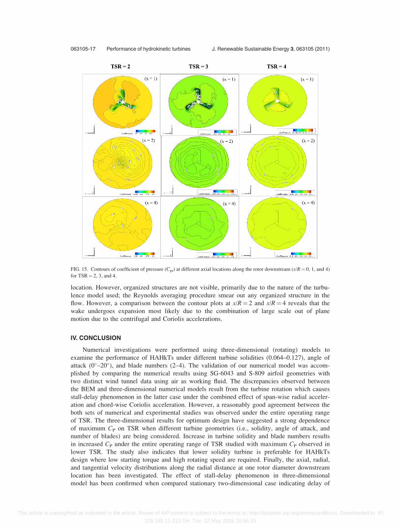
location. However, organized structures are not visible, primarily due to the nature of the turbu-

lence model used; the Reynolds averaging procedure smear out any organized structure in the

flow. However, a comparison between the contour plots at x/R¼ 2 and x/R¼ 4 reveals that the

wake undergoes expansion most likely due to the combination of large scale out of plane

motion due to the centrifugal and Coriolis accelerations.

IV. CONCLUSION

Numerical investigations were performed using three-dimensional (rotating) models to

examine the performance of HAHkTs under different turbine solidities (0.064–0.127), angle of

attack (0–20), and blade numbers (2–4). The validation of our numerical model was accom-

plished by comparing the numerical results using SG-6043 and S-809 airfoil geometries with

two distinct wind tunnel data using air as working fluid. The discrepancies observed between

the BEM and three-dimensional numerical models result from the turbine rotation which causes

stall-delay phenomenon in the latter case under the combined effect of span-wise radial acceler-

ation and chord-wise Coriolis acceleration. However, a reasonably good agreement between the

both sets of numerical and experimental studies was observed under the entire operating range

of TSR. The three-dimensional results for optimum design have suggested a strong dependence

of maximum CP on TSR when different turbine geometries (i.e., solidity, angle of attack, and

number of blades) are being considered. Increase in turbine solidity and blade numbers results

in increased CP under the entire operating range of TSR studied with maximum CP observed in

lower TSR. The study also indicates that lower solidity turbine is preferable for HAHkTs

design where low starting torque and high rotating speed are required. Finally, the axial, radial,

and tangential velocity distributions along the radial distance at one rotor diameter downstream

location has been investigated. The effect of stall-delay phenomenon in three-dimensional

model has been confirmed when compared stationary two-dimensional case indicating delay of

FIG. 15. Contours of coefficient of pressure (Cpr) at different axial locations along the rotor downstream (x/R¼ 0, 1, and 4)

for TSR¼ 2, 3, and 4.

063105-17 Performance of hydrokinetic turbines J. Renewable Sustainable Energy 3, 063105 (2011)

This article is copyrighted as indicated in the article. Reuse of AIP content is subject to the terms at: http://scitation.aip.org/termsconditions. Downloaded to IP:

128.180.11.213 On: Tue, 12 May 2015 19:56:15

separation at further trailing edge of the hydrofoil. In addition, a lesser axial velocity deficit

and, hence, a lesser energy loss at higher TSR further confirm higher CP of HAHkTs.

ACKNOWLEDGMENTS

The authors acknowledge the financial support of Office of Naval Research through Grant No.

N000141010923 (Waves, Wind, and Scavengers: Next Generation Renewable Energy Systems for

Naval Application; Program manager—Michele Anderson) and the Energy Research and Develop-

ment Center at Missouri University of Science & Technology (formerly University of Missouri,

Rolla) for providing the seed-funding for this project.

1J. J. Conti, Annual Energy Outlook 2010: With Projections to 2035, U.S. Energy Information Administration, Office ofIntegrated Analysis and Forecasting, U.S. Department of Energy, Report No. DOE/EIA-0383 (2010).

2I. S. Hwang, Y. H. Lee, and S. J. Kim, Appl. Energy 86, 1532 (2009).3D. Sale, J. Jonkman, and W. Musial, in Proceedings of the 28th ASME International Conference on Ocean, Offshore andArctic Engineering, Honolulu, Hawaii (2009), NREL/CP-500-45021, American Society of Mechanical Engineers, NewYork.

4M. J. Khan, M. T. Iqbal, and J. E. Quaicoe, Renewable Sustainable Energy Rev. 12, 2177 (2008).5M. J. Khan, G. Bhuyan, M. T. Iqbal, and J. E. Quaicoe, Appl. Energy 86, 1823 (2009).6A. Date and A. Akbarzadeh, Renewable Energy 34, 409 (2009).7D. G. Hall, K. S. Reeves, J. Brizzee, R. D. Lee, G. R. Carroll, and G. L. Sommers, Wind and Hydropower Technologies:Feasibility assessment of the water energy resources of the United States for new low power and small hydro classes ofHydroelectric plants, Idaho National Laboratory, DOE-ID-11263(2006).

8S. L. Dixon, Fluid Mechanics and Thermodynamics of Turbomachinery, 5 ed. (Elsevier, Butterworth-Heinemann, MA,2005).

9W. M. J. Batten, A. S. Bahaj, A. Molland, and J. R. Chaplin, Renewable Energy 31, 249 (2006).10L. Myers and A. S. Bahaj, Renewable Energy 31, 197 (2006).11C. A. Consul, R. H. G. Willden, E. Ferrer, and M. D. McCulloch, in Proceedings of the 8th European Wave and Tidal

Energy Conference, Uppsala, Sweden, 2009.12J. F. Manwell, J. G. McGowan, and A. L. Rogers, Wind Energy Explained: Theory, Design and Application. (Wiley, New

York, 2002).13L. J. Vermeer, J. N. Sorensen, and A. Crespo, Prog. Aerosp. Sci. 39, 467 (2003).14J. F. Manwell, J. G. McGowan, and A. L. Rogers, Wind Energy Explained: Theory, Design and Application, 2nd ed.

(Wiley, New York, 2009).15W. M. J. Batten, A. S. Bahaj, A. F. Molland, and J. R. Chaplin, Ocean Eng. 34, 1013 (2007).16W. M. J. Batten, A. S. Bahaj, A. F. Molland, and J. R. Chaplin, Renewable Energy 31, 249 (2006).17W. M. J. Batten, A. S. Bahaj, A. Molland, and J. R. Chaplin, Renewable Energy 33, 1085 (2008).18A. S. Bahaj, W. M. J. Batten, and G. McCann, Renewable Energy 32, 2479 (2007).19L. Myers and A. S. Bahaj, Ocean Eng. 34, 758 (2007).20F. Massouh and I. Dobrev, J. Phys.: Conf. Ser. 75, 012031 (2007).21D. Hu and Z. Du, J. Hydrodynam. 21(2), 285 (2009).22C. Thumthae and T. Chitsomboon, Renewable Energy 34, 1279 (2009).23F. R. Menter, AIAA J. 32(8), 1598 (1994).24F. R. Menter, AIAA J. 30(8), 2066 (1992).25Ansys Fluent 12.0 Theory Guide, Ansys Inc. 2009.26E. Ferrer and X. Munduate, J. Phys.: Conf. Ser. 75, 012001 (2007).27B. Sanderse, Aerodynamics of Wind Turbine Wakes - Literature Review, ECN-E-09-016, Energy Research Center of the

Netherlands (2009).28D. C. Wilcox, Turbulence Modeling for CFD (DCW Industries, La Canada, CA, 1993).29B. E. Launder and D. B. Spalding, Comput. Methods Appl. Mech. Eng. 3, 269 (1974).30P. Giguere and M. S. Selig, J. Sol. Energy Eng. 120, 108 (1998).31M. M. Duquette, J. Swanson, and K. D. Visser, Wind Eng. 27(4), 299 (2003).32M. M. Duquette and K. D. Visser, J. Sol. Energy Eng. 125, 425 (2003).33S. Patankar, Numerical Heat Transfer and Fluid Flow (Hemisphere Publishing Corporation, USA, 1980).34Ansys Fluent 12.0 User’s Guide, Ansys Inc. 2009.35E. P. N. Duque, W. Johnson, C. P. vanDam, R. Cortes, and K. Yee, AIAA Paper No. 2000-0038 (2000).36P. Giguere and M. S. Selig, J. Sol. Energy Eng. 120, 108 (1998).37R. Howell, N. Qin, J. Edwards, and N. Durrani, Renewable Energy 35, 412 (2010).

063105-18 Mukherji et al. J. Renewable Sustainable Energy 3, 063105 (2011)

This article is copyrighted as indicated in the article. Reuse of AIP content is subject to the terms at: http://scitation.aip.org/termsconditions. Downloaded to IP:

128.180.11.213 On: Tue, 12 May 2015 19:56:15