numerical investigation of a phase-change material based

Dissertations and Theses

5-2017

Numerical Investigation of a Phase-ChangeMaterial Based Photovoltaic Panel TemperatureRegulation SystemRohit Gulati

Follow this and additional works at: https://commons.erau.edu/edt

Part of the Mechanical Engineering Commons

This Thesis - Open Access is brought to you for free and open access by Scholarly Commons. It has been accepted for inclusion in Dissertations andTheses by an authorized administrator of Scholarly Commons. For more information, please contact [email protected], [email protected].

Scholarly Commons CitationGulati, Rohit, "Numerical Investigation of a Phase-Change Material Based Photovoltaic Panel Temperature Regulation System"(2017). Dissertations and Theses. 332.https://commons.erau.edu/edt/332

http://commons.erau.edu?utm_source=commons.erau.edu%2Fedt%2F332&utm_medium=PDF&utm_campaign=PDFCoverPages

http://commons.erau.edu?utm_source=commons.erau.edu%2Fedt%2F332&utm_medium=PDF&utm_campaign=PDFCoverPages

https://commons.erau.edu/edt?utm_source=commons.erau.edu%2Fedt%2F332&utm_medium=PDF&utm_campaign=PDFCoverPages

https://commons.erau.edu/edt?utm_source=commons.erau.edu%2Fedt%2F332&utm_medium=PDF&utm_campaign=PDFCoverPages

http://network.bepress.com/hgg/discipline/293?utm_source=commons.erau.edu%2Fedt%2F332&utm_medium=PDF&utm_campaign=PDFCoverPages

https://commons.erau.edu/edt/332?utm_source=commons.erau.edu%2Fedt%2F332&utm_medium=PDF&utm_campaign=PDFCoverPages

mailto:[email protected],%[email protected]

NUMERICAL INVESTIGATION OF A PHASE-CHANGE MATERIAL BASED

PHOTOVOLTAIC PANEL TEMPERATURE REGULATION SYSTEM

by

Rohit Gulati

A Thesis Submitted to the College of Engineering Department of Mechanical

Engineering in Partial Fulfillment of the Requirements for the Degree of

Master of Science in Mechanical Engineering

Embry-Riddle Aeronautical University

Daytona Beach, Florida

May 2017

ii

Acknowledgements

This thesis has been made possible by important contributions made by the thesis

committee members to my life as a graduate student.

Dr. Boetcher has taken me through two heat transfer courses, advised me for my

senior design project, and now guided me through the research for my thesis. I would like

to thank her for all the knowledge she has shared, the criticism she gave when I did

shabby work, and the answers to my many questions she provided even in late night

meetings.

I would like to thank Dr. Compere for sharing his teaching and research methods

with me. He has always been interested in the work I did, provided valuable feedback on

it, and appreciated whenever I made progress.

Finally, I would like to thank Dr. Tang for introducing me to this project in clean

energy, and giving good advice for the direction the project should take.

iii

Abstract

Researcher: Rohit Gulati

Title: Numerical Investigation of a Phase-Change Material Based Photovoltaic

Panel Temperature Regulation System

Institution: Embry-Riddle Aeronautical University

Degree: Master of Science in Mechanical Engineering

Year: 2017

As the production of clean electricity has gained importance, photovoltaic (PV)

panels have become a widely used technology. But, during operation, PV panels heat up

due to the solar insolation and suffer a drop in electrical output. The goal of this

investigation is to use phase-change materials (PCM) to passively cool PV panels. The

PCM is inside an aluminum container attached to the back surface of the PV panel. Four

configurations of the container are investigated. The first configuration is a container

with bulk PCM occupying its entire interior volume. The depth of this container is varied.

The second configuration adds straight aluminum fins to a container of fixed depth. The

length, width and spacing of the fins are parametrically varied. The third configuration

uses an aluminum honeycomb core acting as a fin inside the container. Two cell sizes of

the honeycomb are modelled. The fourth configuration utilizes PCM encapsulated in

pellets, which are suspended in a water bed inside the container. Numerical simulations

are conducted using ANSYS Mechanical APDL for finite element heat conduction. The

solid-to-liquid phase change is modeled using the enthalpy method. A constant heat flux

to simulate the highest value of local irradiance averaged over a day is applied to the

PCM container modules. For all cases, temperatures as a function of time at different

locations of the container are reported. Results show that a deeper container regulates PV

temperature for a longer time. In the finned configuration, as the length of the fins is

increased and the spacing is decreased, the PV surface is maintained at lower

temperatures for longer; fin width only has minimal effect. The honeycomb configuration

matches these criteria and has the lowest PV temperature at PCM saturation time. The

encapsulated configuration performs much worse due to the substantially reduced PCM

volume. A cost function developed to compare the results from different configurations

shows that a honeycomb fin with cell size of 0.5” is most effective at maintaining low PV

temperature for an extended duration.

iv

Table of Contents

Thesis Review Committee ................................................................................................... i

Acknowledgements ............................................................................................................. ii

Abstract .............................................................................................................................. iii

Table of Contents ............................................................................................................... iv

List of Figures ................................................................................................................... vii

List of Tables .................................................................................................................... xii

Chapter I: Introduction and Literature Review ................................................................. 13

Chapter II: Numerical Setup ............................................................................................. 22

2.1 Physical Modelling .................................................................................................. 23

2.1.1 Bulk PCM ......................................................................................................... 24

2.1.1.1 Two-Dimensional Model ........................................................................... 25

2.1.1.2 Three-Dimensional Model ......................................................................... 27

2.1.2 Container with Straight Fins ............................................................................. 28

2.1.2.1 Two-Dimensional Model ........................................................................... 29

2.1.2.2 Three-Dimensional Model ......................................................................... 32

2.1.3 Container with Honeycomb Core Fin ............................................................... 35

2.1.4 Encapsulated PCM ........................................................................................... 40

2.2 Governing Equations and Boundary Conditions ..................................................... 42

v

2.3 Numerical Solution ................................................................................................. 45

2.4 Cost Function .......................................................................................................... 46

Chapter III: Results ........................................................................................................... 48

3.1 Bulk PCM ................................................................................................................ 48

3.1.1 Two-Dimensional Model .................................................................................. 48

3.1.2 Three-Dimensional Model ................................................................................ 50

3.2 Container with Straight Fins ................................................................................... 53

3.2.1 Two-Dimensional Model .................................................................................. 53

3.2.1.1 Case I ......................................................................................................... 54

3.2.1.2 Case II ........................................................................................................ 58

3.2.1.3 Case III ....................................................................................................... 63

3.2.2 Three-Dimensional Model ................................................................................ 68

3.2.2.1 Case I ......................................................................................................... 68

3.2.2.2 Case II ........................................................................................................ 70

3.3 Container with Honeycomb Core Fin ..................................................................... 72

3.3.1 Case I ................................................................................................................ 72

3.3.2 Case II ............................................................................................................... 76

3.4 Encapsulated PCM .................................................................................................. 78

3.5 Cost Comparison ..................................................................................................... 80

Chapter IV: Conclusions and Future Work ...................................................................... 84

vi

Appendix A ....................................................................................................................... 89

Appendix B ....................................................................................................................... 92

Appendix C ....................................................................................................................... 95

Appendix D ....................................................................................................................... 98

References ....................................................................................................................... 102

vii

List of Figures

Figure 1.1: Output power versus voltage of a single crystalline silicon solar cell at various

temperatures ...................................................................................................................... 15

Figure 2.1: Schematic of the PCM container as it attaches to the back of the PV panel .. 22

Figure 2.2: Schematic diagram of the PCM container and the lid used in simulations .... 24

Figure 2.3: Schematic of bulk PCM in the container........................................................ 25

Figure 2.4: Two-dimensional cross section of the bulk PCM configuration as used in the

simulations ........................................................................................................................ 26

Figure 2.5: Yellow wedge shows a schematic of the geometry used in 3D simulations of

the bulk PCM configuration.............................................................................................. 27

Figure 2.6: (left) A top view of the 3D geometry simulated, showing the three sites of

interest. (right) The same wedge as seen from the right, showing sites 𝑆2 and 𝑆3, along

with the temperature monitor locations at these sites ....................................................... 28

Figure 2.7: Schematic diagram of the PCM container with straight fins. ......................... 29

Figure 2.8: Two-dimensional cross section of the finned container configuration as used

in the simulations...............................................................................................................30

Figure 2.9: Yellow block shows a schematic of the geometry used in 3D simulations of

the finned PCM container configuration........................................................................... 33

Figure 2.10: Top view of the quarter model of finned container, Case II ........................ 34

Figure 2.11: Back view of the geometry of the finned container Case II ......................... 35

Figure 2.12: Schematic diagram of the PCM container with a honeycomb core fin. ....... 36

viii

Figure 2.13: Dimensions of the honeycomb core used in Case I...................................... 37


the configuration with a honeycomb core fin inside the PCM container. ........................ 37

Figure 2.15: Dimensions of the honeycomb core used in Case II .................................... 38

Figure 2.16: Top view of the quarter model of container with honeycomb fin, Case I .... 39

Figure 2.17: Encapsulated PCM pellets ............................................................................ 40

Figure 2.18: Schematic diagram of the PCM container with encapsulated PCM pellets . 41


the encapsulated PCM configuration. ............................................................................... 42

Figure 3.1: Temperature contour plot at PCM saturation of a 2D geometry of the bulk

PCM configuration............................................................................................................ 49

Figure 3.2: Plots of PV temperature versus time for different depths of the PCM

container. ........................................................................................................................... 50

Figure 3.3: Plots of PV temperature versus time for the 2D model and 3 sites of the 3D

model of bulk PCM configuration .................................................................................... 51

Figure 3.4: Temperature contours of the 3D model of the bulk PCM container at PCM

saturation time ................................................................................................................... 52

Figure 3.5: PV temperature versus time for varying fin lengths obtained from the 2D

model of finned container..................................................................................................54

Figure 3.6: Plots of location 𝐿2 (inside bottom surface) versus time for varying fin

lengths ............................................................................................................................... 55

ix

Figure 3.7: Temperature contours at PCM saturation time for different fin lengths ........ 56

Figure 3.8: PCM saturation time and corresponding PV temperature for different fin

lengths. .............................................................................................................................. 57

Figure 3.9: 𝐿1 temperature plots for finned container Case II.......................................... 59

Figure 3.10: 𝐿5 temperature plots for finned container Case II ........................................ 60

Figure 3.11: 𝐿1 temperature plots for finned container Case II. ....................................... 61

Figure 3.12: 𝐿5 temperature plots for finned container Case II. ....................................... 62

Figure 3.13: 𝐿1 temperature plots for finned container Case III. ..................................... 63

Figure 3.14: 𝐿6 temperature plots for finned container Case III ...................................... 65

Figure 3.15: Plots of PCM saturation time and PV temperature at this time for varying fin

width and spacing in Cases II and III. ............................................................................... 66

Figure 3.16: Temperature plots of location 𝐿1 obtained from the 2D model, and six sites

of the 3D model ................................................................................................................ 69

Figure 3.17: Temperature contours at full melt for honeycomb configuration Case I ..... 73

Figure 3.18: Temperature plots of location 𝐿6 obtained from the 3D cases of finned

configuration, and four cells of the honeycomb configuration Case I. ............................. 74


configuration, and four cells of the honeycomb configuration Case I. ............................. 75


configuration, and four cells of the honeycomb configuration Case II. ........................... 77

x

Figure 3.21: Temperature contours at PCM saturation time for quarter model of

encapsulated PCM configuration. ..................................................................................... 79

Figure 3.22: Plot of PV temperature versus time for encapsulated PCM configuration. . 80

Figure 3.23: PV temperature plots for different PCM container configurations .............. 81

Figure 3.24: Graphical comparison of performance metrics ............................................ 82

Figure A.1: 𝐿1 temperature plots for finned container Case II ......................................... 89






Figure B.1: 𝐿1 temperature plots for finned container Case II ......................................... 92






Figure C.1: 𝐿1 temperature plots for finned container Case III........................................ 95



xi




Figure D.1: 𝐿1 temperature plots for finned container Case III ....................................... 98




Figure D.5: 𝐿6 temperature plots for finned container Case III ..................................... 100




xii

List of Tables

Table 2.1: Different cases of the finned container are modelled by varying fin dimensions

in the 2D geometry. Values of for each case are shown below. ....................................... 31

Table 2.2: Temperature monitor locations in the 2D model of finned container

configuration. .................................................................................................................... 32

Table 2.3: Material properties of PureTemp 29. ............................................................... 43

Table 2.4: Enthalpy values of PureTemp 29 used in simulations. .................................... 44

Table 2.5: Material properties used in simulations ...........................................................44

Table 3.1: Results from different depths of container modelled as 2D geometries for bulk

PCM configuration............................................................................................................ 49

Table 3.2: Results from Case I of 3D models for finned PCM configuration compared to

equivalent 2D model. ........................................................................................................ 70

Table 3.3: Results from Case II of 3D models for finned PCM configuration compared to

equivalent 2D model. ........................................................................................................ 71

Table 3.4: Results from two 3D cases of finned PCM configuration compared to

honeycomb configuration Case I. ..................................................................................... 76


honeycomb configuration Case II. .................................................................................... 78

Table 3.6: Costs for various container configurations. ..................................................... 81

13

Chapter I

Introduction and Literature Review

An ample supply of electricity is essential to the modern world. Lighting, air

conditioning, refrigeration, medical equipment, water supply, computing, and

transportation are a few major areas which have developed along with, and thus, reliant

on electric supply. Today, an additional strain on the power grid is being added in the

form of personal transportation – electric cars. Traditionally, electricity has been

produced by power stations that burn fossil fuels such as coal, oil, and natural gas.

According to the United States Energy Information Administration, about 67% of the

electricity generated in the US in 2015 was from fossil fuels [1].

Recently, there has been a shift towards using alternate sources of energy for the

production of electricity due to four reasons. First, there is a growing concern over

climate change, which is accelerated by the greenhouse gas emissions from burning fossil

fuels. Second, burning fossil fuels also generates particulate emissions, which have a

negative impact on air quality. Third, fossil fuels are a non-renewable resource, which

means they are not a viable electricity generation source for long term energy security.

And fourth, to meet the growing demand of electricity more generating capacity is being

added to the power grid and new resources are being exploited. 2016 saw the US power

grid generating capacity increase by 15 GW, which is the largest net change in 5 years

[2].

14

One of the primary alternate technologies for electricity generation is the use of

photovoltaic panels to capture solar energy. PV panels make us of the photovoltaic effect

exhibited by some semiconducting materials to generate an electric potential from

sunlight. This method of generating electricity creates no greenhouse gas or particulate

emissions. Also, solar irradiance is a free and renewable energy resource, which makes it

an appealing option.

While PV panels are widely used to generate clean electricity, they are only

approximately 10-16% efficient in converting incident solar irradiance into electricity.

This is because the photovoltaic cells, which are linked together to form a solar panel,

produce electricity from a specific range of light frequencies. All remaining frequencies

in solar irradiance are unused. This remaining incident energy turns to heat and raises the

temperature of the PV panels. As the temperature increases, the electrical output of the

panels drops, thereby decreasing the efficiency. Different researchers have shown that a

crystalline silicon PV panel operating above 25°C shows a temperature-dependent power

decrease with a coefficient between 0.4%/K and 0.65%/K [3-5]. Thus, lowering the

operating temperature of a PV panel can lead to a significantly improved electrical

output, as shown in Figure 1.1.

15

Several methods of thermal regulation have been developed in order to prevent

the drop in electrical output of PV panels caused by an increase in operating temperature.

PV panels may be passively or actively cooled. Passive cooling usually relies on natural

convection heat transfer due to the circulation of air in the open space behind the PV

panel. While this cooling method has some benefits ground mounted and roof mounted

PV panels, building integrated photovoltaics (BIPVs) are not inherently able to take

advantage of this type of cooling due to the restricted space behind the panels. According

to Krauter et al., in the absence of this passive cooling mechanism BIPVs yield a 9.3%

lower electrical output when compared to non-integrated PV panels [6]. Active cooling

can be used for all kinds of PV panel installations, but consumes energy to pump a fluid

(usually water) over the front or back surface of the PV panel.

Figure 1.1: Output power versus voltage of a single crystalline silicon solar cell at various

temperatures [5].

16

When the temperature regulation system stores the waste heat, which is then used

for thermal work, the system is called a photovoltaic/thermal (PVT) hybrid collector.

Liquid- and air-cooled PVT and BIPVT hybrid collectors have been studied extensively

[7, 8]. However, using phase-change material (PCM) as the heat sink in PVT or BIPVT

systems is an emerging technology that has recently gained attention, as detailed in the

review conducted by Ma et al. [9].

Phase change material is engineered to absorb large amounts of latent heat over a

very narrow temperature band. Thus, if there is good thermal contact between the PCM

and the PV panel, a PCM-based temperature regulation system should be able to maintain

the PV panel at near-constant temperature while the PCM absorbs the waste heat from the

panel and changes phase. The heat energy stored in the PCM can then either be removed

through a heat exchanger, or utilized for other applications.

One of the earliest studies of PCM affixed to a PV panel was conducted by

Häusler and Rogaß in 1998 [10]. Häusler and Rogaß used a glass tank filled with water,

inside which there was PCM placed in polyethylene spheres. Poor heat transport from the

PV panel to the PCM was seen due to the small contact area and poor thermal contact

caused by the bad thermal conductivity of the spheres. A second design was also tested,

with the PCM now encased in flat copper tanks, again placed in the water filled glass

tank. This time, good heat transport was seen, but tanks were destroyed due to the

corrosive nature of the PCM and the volume changes caused with a change in phase. The

system was improved later with a new design which featured an aluminum absorber [11].

The photovoltaic cells are laminated directly onto one side of the absorber, while the

other side has a tank filled with PCM.

17

In 2004 Huang et al. were able to develop one of the first numerical models of a

system that uses PCM to moderate the temperature of a PV panel [12]. This model was

then validated with results from experiments conducted using similarly sized geometries.

The effect of adding metal fins to the system was also studied. This showed a significant

improvement in the thermal performance of the regulation system. In 2006, Huang et al.

presented further experimental evaluation of PV-PCM systems that utilized internal fins

[13]. For three different systems, the numbers, dimensions, and forms of fins for two

PCMs were investigated. All of the PCM assisted finned systems showed improvement

over a finned PV panel cooled by natural ventilation. The same researchers also

published a study that compared results from a three-dimensional (3D) model of a PV-

PCM system to the two-dimensional (2D) model presented in their earlier work. A good

agreement was found between the two numerical modelling approaches [14].

One of the first BIPV systems using PCM as a heat sink was built and tested at

Oak Ridge National Laboratory by Kosny et al. in 2009 [15, 16]. Amorphous silicon PV

laminates and PCM heat sinks were integrated into metal panels to be placed on the roof.

During the winter, the roof acted as a passive solar collector where the PCM stored solar

heat in the day, which was released in the night to reduce building heating loads. During

the summer, the PCM in the roof acted as a heat sink, reducing the heat gained by the

interior of the house. The investigators focused on thermal characteristics of the PCM

during solar heating rather than the efficiency of the PV panels. They found that the PV-

PCM roof generated cooling loads that were approximately 55% lower than a standard

shingle roof; and during the winter, the PV-PCM roof generated heating loads that were

about 30% less than a standard shingle roof.

18

In 2010, Hasan et al. [17] performed a comparative study of the effect of various

PV-PCM systems on the PV panel temperature. Five PCMs were used in the study, which

were enclosed in four different kinds of containers attached to the photovoltaic cell to

form the PV-PCM system. The containers varied in materials and thicknesses. The

performance of each design was evaluated at three solar insolation intensities. It was

found that a maximum temperature reduction of 18°C was achieved for 30 minutes.

In 2011, Huang et al. tried to overcome the limited effectiveness of PCM heat

sink due to their low thermal conductivities and crystallization segregation during

solidification [18]. They experimentally investigated the effect of natural convection in

finned PCM heat sinks.

Biwole et al. [19] developed a finite-element model of an impure PCM coupled

with a PV panel, and compared isotherms from numerical experiments to an experimental

setup. In this study, published in 2013, the researchers found that with the addition of the

PCM, the operating temperature of the PV panel remained under 40°C for 80 minutes.

Without the use of PCM, the PV panel reached this temperature after only 5 minutes. In

2014, Lo Brano et al. [20] developed a finite-difference thermal model of PCM, which

solved two sets of recursive equations for two spatial domains in the PV-PCM system: a

boundary domain and an internal domain. The model was validated experimentally under

varied weather conditions.

Also, around the same time, Park et al. [21] evaluated the power performance of a

BIPV-PCM panel system. The experimental setup consisted of a PV panel with attached

PCM heat sink, which was mounted on a rooftop. Along with being exposed to varied

19

ambient temperatures, insolation, and wind speeds throughout the experiment, different

orientations of the PV panel were also introduced. The researchers found that the

electrical power output of the PV increased by 3% when the amount of vertical solar

radiation was high and when the outdoor air temperature was moderate. An electro-

thermal simulation of the combined system, exposed to the same weather conditions as

the experiment, was also set up in TRNSYS. Reasonable agreement between the

experimental and predicted values of PV temperature and electric power output was seen.

Aelenei et al. [22, 23] developed a one-dimensional heat transfer model coupled

with experimental verification to study a prototype BIPV-PCM system. This system was

installed on the main façade of a building. While the PV panel forms the outer layer

exposed to sunlight, the PCM is embedded into a gypsum insulating board behind the

panel. However, the panel and PCM are not in direct thermal contact since there is an air

gap of variable width between the two. Their results show an overall combined electrical

and thermal efficiency of around 20%.

Maiti et al. [24] proposed a V-trough PV-PCM system and determined the

effectiveness of using a paraffin wax-based PCM with a melt temperature between 56-

58°C. Metal turnings were embedded into the low-thermal conductivity PCM to promote

heat flow through it. Their experiments determined that indoors, the PV temperature was

reduced by approximately 25°C for 3 hours, and outdoors, the temperature was reduced

by 16°C. The outdoor temperature reduction could be sustained for the entire operating

day.

20

In 2015, Hasan et al. [25] compared the effect of utilizing PCM on the back of PV

panels in two different climates: Dublin and Vehari. Two separate PCMs were used in the

study – a salt hydrate and a eutectic mixture of two fatty acids. They concluded that the

PCM was more effective in regulating the temperature of PV panels in the hotter climate

of Vehari, which also gets stable radiation throughout the year. The gains from using the

PCM were smaller when in the overcast and cooler climate of Dublin. Also, at both

testing sites, the salt hydrate PCM achieved a greater drop of PV panel temperature.

Recently, Sharma et al. experimentally determined the performance of a building-

integrated concentrating photovoltaic system thermally regulated with PCM [26]. The

system was validated at four different irradiance levels, ranging from 500W/m2 to 1200

W/m2. Their highly controlled indoor experiments found that, for all irradiance levels,

incorporating PCM resulted in an increase in electrical efficiency and a decrease in the

panel temperature. The maximum improvement was seen with a 1000 W/m2 irradiance,

where the use of PCM increased the electrical efficiency by 7.7% and lowered the

module center temperature on average by 3.8°C when compared to a standard system.

Almost all the studies on PCM assisted thermal regulation systems have used bulk

PCM solidified in a container. Utilizing a slightly different approach to PCM packaging,

Ho et al. [27-31] implemented microencapsulated phase change material (MEPCM) as a

means of improving the efficiency of BIPVs. In [27], Ho et al. modeled the MEPCM

embedded in a fluid as a buoyancy-driven natural convection problem in a porous media.

They determined that the MEPCM layer increased the efficiency by as much as 0.42 %.

Follow-on numerical studies by the same authors [28-31] model different MEPCM layer

21

configurations and show the promise of using MEPCM in a fluid bed for BIPV thermal

regulation and energy storage.

The literature reviewed shows that experimental design, testing, numerical model

development, and performance evaluation of PV-PCM systems have constituted many

recent efforts. This thesis presents the work done to achieve the same goal of limiting the

increase of PV panel temperature in order to prevent a drop in electrical output by using a

PCM based temperature regulation system. Geometries of the different configurations of

an organic based PCM are modelled. The PCM melt characteristics are modelled based

on the enthalpy method. The same boundary conditions are then applied to each design

and then solved numerically using a finite element solver with the same boundary

conditions to investigate the effectiveness of the PCM heat sink. Temperatures of various

locations in the solution domain are monitored to gain an understanding of the melt

process of the PCM. PCM saturation time and PV panel temperature for the different

designs are compared. To evaluate the performance of different regulation system

configurations, a cost function is developed. The most effective configuration would be

the one closest to ideal, and thus, have minimal cost.

22

Chapter II

Numerical Setup

Through review of past literature, it is seen that a PCM heat sink can be used as a

passive temperature regulation system for PV panels. But, there are various ways to

implement this idea. To supplement the experimental studies being performed in the

laboratory by other researchers, numerical simulations of four different configurations of

the PCM are set up. The PCM is inside a container attached directly to the back surface

of the PV panel, as shown in Figure 2.1. By comparing the PV panel temperature over

time, the effectiveness of different PCM configurations can be gauged.

Figure 2.1: Schematic of the PCM container as it attaches to the back of the PV panel.

23

2.1 Physical Modelling

Before a cooling system is designed for a full-size PV panel, initial studies are

focused on regulating the temperature of a small, 15 W PV panel with an area of 929

cm2. Upon inspection of the 15 W PV panel, it is determined that the cooling area on the

back of the panel would have a footprint of 10” by 10” (25.4 cm by 25.4 cm).

The PV panel is not modelled in the simulations because the exact thermal

properties of it are not known. Instead, the back surface of the panel is assumed to be in

perfect thermal contact with a 1/8” (3.175 mm) thick plate of aluminum. Behind this plate

is the PCM container with inner dimensions of 10” by 10”. The container is made of 1/8”

thick plates of aluminum as well. This material was chosen for its lightness and good

thermal conductivity which would allow heat to travel away from the PV panel with little

resistance. Through experiments in the laboratory, and past use in a cold plate for the

energy storage system of an EcoCAR2 vehicle [32], it is determined that despite its

corrosive nature, the organic based PCM used in this study is compatible with the

aluminum container. Figure 2.2 shows the arrangement of the container and the lid

attached to the PV panel, as used in simulations.

24

Figure 2.2: Schematic diagram of the PCM container and the lid used in simulations. The

PV panel rests on top of the lid, and perfect thermal contact is assumed between them.

With the chosen model of the PV panel and PCM container design, there are four

main configurations of the PCM and its container that are numerically solved.

2.1.1 Bulk PCM

The first design consists of just the aluminum container filled with PCM and its

lid attached to the back of the PV panel, as shown in Figure 2.3.

10.25” 10.25”

0.125”

Aluminum sheet

in contact with PV

panel back surface

PCM container

25

Figure 2.3: Schematic of bulk PCM in the container.

In this configuration, the PCM is also in direct thermal contact with the aluminum

sheet that lines the back surface of the PV panel. This configuration was simulated as

two- and three-dimensional models.

2.1.1.1 Two-Dimensional Model

The 2D model of the bulk PCM configuration assumes an infinitely large

container, and takes advantage of thermal symmetry to reduce the solution domain to a

cross section of the actual design. Figure 2.4 shows the geometry used in these 2D

simulations.

PCM container

Aluminum sheet

in contact with PV

panel back surface PCM

26

Figure 2.4: Two-dimensional cross section of the bulk PCM configuration as used in the

simulations. 𝐿1 and 𝐿2 are the temperature monitor locations.

The width of the cross section is held constant at 1” (25.4 mm), while the internal

depth of the container, 𝑑, is varied. Three depths are modelled – 1/3” (8.467 mm), 1/2”

(12.7 mm), and 1” (25.4mm). The container’s internal depth is restricted to a maximum

of 1” so that the design can be scaled up and implemented on the back of any full sized

PV panel without interfering with the rack mounting system. Temperature was monitored

at two locations in this 2D model, as marked in Figure 2.4. 𝐿1 is the temperature of the

back surface of the PV panel, and 𝐿2 is the temperature of the inside bottom surface of

the container.

27

2.1.1.2 Three-Dimensional Model

Only a PCM depth of 1” is modelled for the 3D simulations of the bulk PCM

configuration. This model utilizes physical symmetry of the design to reduce the solution

domain. A one-eighth section of the container, lid, and PCM is modelled, shown as a

yellow wedge in Figure 2.5. The two sides perpendicular to each other are of length

5.125” (130.175 mm). With the internal depth of the PCM container set to 1”, the total

height of the wedge is 1.25” (31.75 mm).

Figure 2.5: Yellow wedge shows a schematic of the geometry used in 3D simulations of

the bulk PCM configuration.

Figure 2.6 shows the three sites in this 3D model that are chosen for temperature

data collection. At each of these three sites, temperatures are monitored at two locations

along the height of the geometry – the back surface of the PV panel and the inside bottom

5.125”

45° 1.25”

28

surface of the container. These locations are analogous to 𝐿1 and 𝐿2 from the two-

dimensional model, respectively.

Figure 2.6: (left) A top view of the 3D geometry simulated, showing the three sites of

interest. (right) The same wedge as seen from the right, showing sites 𝑆2 and 𝑆3, along

with the temperature monitor locations at these sites.

2.1.2 Container with Straight Fins

The second configuration investigated utilizes PCM inside the aluminum

container with an internal depth of 1”. In addition, to enhance heat flow from the PV

panel surface into the PCM, straight aluminum fins are placed in the container. Figure 2.6

shows a schematic of this design.

PCM

Lid

Container

29

Figure 2.7: Schematic diagram of the PCM container with straight fins. Dimensions 𝑠 and

𝑤 represent fin spacing and fin width, respectively.

The aluminum fins in this configuration are attached to the aluminum sheet that

lines the back surface of the PV panel, and span the entire length of the container.

Different fin lengths, 𝑙, fin widths, 𝑤, and fin spacings, 𝑠, are investigated. The PCM is in

contact with the container lid, and also the straight aluminum fins. This configuration was

also simulated as two- and three-dimensional models.

2.1.2.1 Two-Dimensional Model

The 2D model of the finned PCM container configuration assumes an infinitely

large container, and takes advantage of thermal and geometric symmetry to reduce the

solution domain to a cross section of the actual design. Figure 2.8 shows the geometry

used in these 2D simulations.

PCM container

PCM

Aluminum sheet

in contact with PV

panel back surface

Straight

aluminum

fins

s

w

30

Figure 2.8: Two-dimensional cross section of the finned container configuration as used

in the simulations. 𝐿1 through 𝐿6 are the temperature monitor locations. Dimensions 𝑙, 𝑠,

and 𝑤 represent fin length, fin spacing and fin width, respectively.

The internal depth of the container, 𝑑, is held constant at 1” (25.4 mm), while

three other parameters – 𝑙, fin length, 𝑤, fin width, and 𝑠, fin spacing – are parametrically

varied to study the effect on PV panel temperature. Table 2.1 lists the variations in these

dimensions in the three cases simulated.

31

Table 2.1: Different cases of the finned container are modelled by varying fin dimensions

in the 2D geometry. Values of for each case are shown below.

Dimension Case I Case II Case III

Fin length, 𝑙 [mm] 0 – 25.4 13 25.4

Fin width, 𝑤 [mm] 1 1, 1.5, 2, 3.175 1, 1.5, 2, 3.175

Fin spacing, 𝑠 [in] 1 0.5, 1, 1.5, 2 0.5, 1, 1.5, 2

In Case I, the fin spacing is held constant at 1”, and the length of a 1 mm wide

aluminum fin attached to the top plate is varied until it reaches the bottom plate. In Case

II, the fin length is held constant at 13mm, while combinations of different fin widths and

fin spacing are simulated. Case III is similar to Case II with varied fin width and spacing,

but the length of the fin is 25.4 mm so that it connects the top and bottom aluminum

plates of the PCM container. Figure 2.8 also shows the locations where temperature was

monitored in the 2D model of the finned container. Table 2.2 describes them in more

detail.

32

Table 2.2: Temperature monitor locations in the 2D model of finned container

configuration.

Location Description

L1 Back surface of the PV panel/outer surface of the

container lid

L2 Inside bottom surface of the container

L3 Fin tip

L4 PCM (top) – adjacent to the top plate, and halfway

between two fins

L5 PCM (bottom) – adjacent to the bottom plate, and

halfway between two fins

L6 PCM (middle) – halfway (0.5”) along the depth of

the container, and halfway between two adjacent fins

2.1.2.2 Three-Dimensional Model

This model utilizes physical symmetry of the design to reduce the solution

domain. A one-fourth section of the finned container, lid, and PCM is modelled, shown

as a yellow block in Figure 2.9. The length and width of this square section are both

5.125” (130.175 mm) long. With the internal depth of the PCM container set to 1”, the

total height of the block is 1.25” (31.75 mm).

33


the finned PCM container configuration.

Only two particular cases are modelled as 3D geometries. This is mainly done to

compare with results from the 2D simulations and check if the walls of the container,

which were not modelled in the 2D geometry, have a significant impact on heat flow.

Both cases have fins of length 1”, so that they connect the top and bottom plated of the

PCM container. In Case I, the fins have a width, 𝑤, of 1mm, and are arranged with a

spacing, 𝑠, of 0.5”. Thus, the entire container is able to fit 19 fins in it, while the quarter

model used for simulations has 10 of these fins. In Case II, the fins have a width, 𝑤, of

3.175 mm (1/8”), and are evenly spaced 1” apart. Thus, the entire container is able to fit 9

fins in it, while the quarter model has 5 of these fins.

1.25”

5.125”

5.125”

34

Six sites of interest are chosen in the quarter model. Since cases I & II have fins

which connect the top and bottom plates and span the length of the box, the PCM is

effectively divided into separate blocks. Sites 𝑆1, 𝑆2, and 𝑆3 are located such that the

PCM block adjacent to the container wall, and the fin adjacent to it, fall within them.

Sites 𝑆4, 𝑆5, and 𝑆6 include the central fin of the PCM container, and the PCM block

adjacent to it. Figure 2.10 shows a top view of the geometry used in Case II, with the

temperature collection sites highlighted. Three slicing planes passing through the sites are

also shown.

Figure 2.10: Top view of the quarter model of finned container, Case II. All dimensions

are drawn to scale. Three slicing planes (dashed orange lines) pass through the PCM

blocks to give six sites of interest. Sites 𝑆1 through 𝑆6 are highlighted in yellow.

S3

S2

S1 S4

S5

S6

35

At each of the sites 𝑆1 through 𝑆6, a plane parallel to the bottom edge of the

container is used to slice the 3D geometry and reveal cross sections similar to the 2D

model of Figure 2.8. Temperatures are monitored at locations 𝐿1 through 𝐿6, analogous

to the 2D model locations. Figure 2.11 shows a back view of the quarter model of Case

II, with sites 𝑆3 and 𝑆6 visible. Temperature collection locations for site 𝑆6 are marked

𝐿1 through 𝐿6.

Figure 2.11: Back view of the geometry of the finned container Case II. All dimensions

are drawn to scale. Site 𝑆6 from Figure 2.10 is visible, with the temperature monitor

locations 𝐿1 through 𝐿6 marked.

2.1.3 Container with Honeycomb Core Fin

For the third configuration investigated a PCM container with an internal depth of

1” is used. A honeycomb core made of aluminum is inserted into the container and acts

as a fin to improve heat transfer from the PV surface to the PCM. The honeycomb also

has a depth of 1”, connecting the top and bottom plates of the PCM container, dividing

the PCM in to separate cells. Figure 2.12 shows a schematic of this design.

S6

36

Figure 2.12: Schematic diagram of the PCM container with a honeycomb core fin. The

depth of the honeycomb core is 1”.

Two cases are investigated with different sizes of the honeycomb core. Case I is

modelled on the commercially available honeycomb core from McMaster-Carr (Part#

9365K511). A manufacturer provided cell size of 1” (25.4 mm) and a measured foil

thickness of 0.2 mm are used to create the geometry of the fin. Figure 2.13 shows a close-

up of the honeycomb. 10 honeycomb cells fit horizontally inside the PCM container.

Figure 2.14 shows how symmetry is used to reduce the solution domain to one fourth of

the container, similar to the finned design. The quarter model contains 5 honeycomb cells

horizontally.

Aluminum sheet

in contact with PV

panel back surface

PCM container

PCM

Aluminum

honeycomb

core fin

37

Figure 2.13: Dimensions of the honeycomb core used in Case I. The depth of the

honeycomb is 1” (25.4 mm).


the configuration with a honeycomb core fin inside the PCM container.

1.25”

5.125”

5.125”

38

Case II of the honeycomb fin design is a modification of Case I. The cell size of

the honeycomb is reduced to 0.5” (12.7 mm) to check if distributing the PCM into

smaller cells has an effect on the temperature regulation of the PV panel. A close-up of

the honeycomb used in Case II is shown in Figure 2.15. With a cell size of 0.5”, 20

honeycomb cells fit horizontally inside the PCM container. Again, symmetry is used to

reduce the solution domain to a quarter model containing 10 honeycomb cells

horizontally.

Figure 2.15: Dimensions of the honeycomb core used in Case II. The depth of the

honeycomb is 1” (25.4 mm).

Temperatures of four PCM cells in the quarter model are monitored. These cells

are labeled 𝐵𝐿 (bottom left), 𝐵𝑅 (bottom right), 𝑇𝐿 (top left), and 𝑇𝑅 (top right) based on

their locations in the quarter model. Figure 2.16 shows the geometry used for Case I with

the cells of interest marked.

39

Figure 2.16: Top view of the quarter model of container with honeycomb fin, Case I. All

dimensions are drawn to scale. Two slicing planes (dashed orange lines) pass through the

centroids of PCM cells highlighted in yellow to give four cells of interest. Cell 𝐵𝐿 was

chosen slightly away from bottom left position so that its centroid doesn’t fall on the

sidewall.

Slicing planes parallel to the bottom edge of the PCM container are passed

through the centroids of the four cells to reveal cross sections. These cross sections are

treated like the one shown in Figure 2.8. For each cell, temperatures of six locations 𝐿1

through 𝐿6 are monitored.

TR

BR

TL

BL

40

2.1.4 Encapsulated PCM

While all configurations modelled until now have had the PCM poured directly

into the aluminum container, this design uses PCM in encapsulated form. The PCM is

encapsulated inside pellets made of a blend of plastics that are resistant to its corrosive

properties. Each pellet has a diameter of 18 mm (0.71”) with a 3 mm (0.12”) halo, as

shown in Figure 2.17. The halo is due to the sealing in the manufacturing process. The

thickness of the wall is measured as 0.45 mm (0.012”).

Figure 2.17: Encapsulated PCM pellets [33].

169 pellets are uniformly arranged in a container with 1” internal depth to form a

single layer. The container is filled with water to occupy the remaining volume and

provide a medium for heat to travel from the container walls into the pellets. To make the

modelling process easier, the dimples and the halo found on the pellets are not modelled.

The pellets are thus modelled as thin walled spheres with PCM occupying their entire

41

interior volume. The encapsulating material is assigned properties of high-density

polyethylene (HDPE). Figure 2.18 shows a schematic of this design.

Figure 2.18: Schematic diagram of the PCM container with encapsulated PCM pellets.

Symmetry is used to reduce the solution domain and model only one quarter of

the encapsulated PCM configuration, as shown in figure 2.19. There are 49 pellets in the

reduced geometry. Only one site at the top right corner of the quarter model (or, the

center of the entire PCM container) is chosen for collection of temperature data. At this

site, temperatures of the PV panel and the inner surface of the bottom plate are

monitored. PCM temperature at the center of the pellet that is at this site is also recorded.

Aluminum sheet

in contact with PV

panel back surface

PCM container

PCM

HDPE pellet

casing

42


the encapsulated PCM configuration.

2.2 Governing Equations and Boundary Conditions

The PCM used in numerical experiments is a proprietary blend of organic based

fatty acids, called PureTemp 29. It is sold commercially by Entropy Solutions, LLC. The

melting temperature range of this PCM is 27.6°C to 29.6°C. This saturation temperature

was chosen to be higher than the average outdoor temperature of Daytona Beach, and

lower than the peak operating temperature of PV panels. Because of this, the PCM’s

latent heat would not be used up in just reaching thermal equilibrium with the ambient

air. Instead, the latent heat would be drawn from the hot PV panel, effectively regulating

the panel’s temperature. Material properties of PureTemp 29 obtained from the

manufacturer are shown in Table 2.3.

5.125”

5.125”

1.25”

43

Table 2.3: Material properties of PureTemp 29.

Property Value

solid phase liquid phase

Density, 𝜌 [𝑘𝑔 𝑚3⁄ ] 940 850

Specific Heat Capacity, 𝑐𝑝 [𝐽 𝑘𝑔 ∙ 𝐾⁄ ] 1770 1940

Thermal Conductivity, 𝑘 [𝑊 𝑚 ∙ 𝐾⁄ ] 0.25 0.15

Melting Temperature Range [°𝐶] 27.6 – 29.6

Latent Heat of Fusion, ℎ [𝐽 𝑘𝑔⁄ ] 202,000

For all four configurations of the PCM, the solid-to-liquid phase change is

modeled using the enthalpy method developed by Shamsundar and Sparrow [34]. This is

a lumped method that does not take into account the interface between the solid phase

and the liquid phase, nor the natural convection present in the melt. However, this model

has proven to be reasonably accurate at predicting temperature during the phase change.

Also, in the encapsulated PCM container, natural convection of the water caused by

temperature gradients while the container and its contents heat up is neglected. This is

done because the small gaps between the pellets, and between the pellets and the

container walls would not let steady convection currents form. In addition, there would

not be a very large temperature gradient along the depth of the PCM container.

Using the enthalpy method, the conservation of energy equation in the completely

solid solution domain is solved numerically.

𝜕ℎ

𝜕𝑡= 𝑘 [

𝜕2𝑇

𝜕𝑥2+

𝜕2𝑇

𝜕𝑦2+

𝜕2𝑇

𝜕𝑧2] (2.1)

44

In Eq. 2.1, ℎ is enthalpy, 𝑡 is the time, 𝑘 is thermal conductivity, T is the temperature, and

x, y, and z are Cartesian coordinates.

An arbitrary datum for the enthalpy of the PCM is specified at 0°C, and the

enthalpies per unit volume for other temperatures are calculated and entered as inputs to

the numerical solver. These enthalpy values are listed in Table 2.4.

Table 2.4: Enthalpy values of PureTemp 29 used in simulations.

Temperature [°𝐶] Enthalpy, 𝒉 [𝐽/𝑚3]

0 0

27.6 45,920,880

29.6 230,031,330

50 263,670,930

Material properties of the other materials used in the different configurations are

listed in Table 2.5. While the properties of HDPE were aggregated from Matbase, the

properties of aluminum and water were obtained from [35].

Table 2.5: Material properties used in simulations.

Property Aluminum HDPE Water

Density, 𝜌 [𝑘𝑔 𝑚3⁄ ] 2700 974 997

Specific Heat Capacity, 𝑐𝑝 [𝐽 𝑘𝑔 ∙ 𝐾⁄ ] 903 2250 4180

Thermal Conductivity, 𝑘 [𝑊 𝑚 ∙ 𝐾⁄ ] 237 0.49 0.618

45

In order to model the worst case scenario for the temperature regulation system,

all external boundaries except the surface in contact with the PV panel are modelled as

adiabatic. This way, all the incoming heat will be stored in the container and the PCM

within.

A constant heat flux of 525 W/m2 is applied to the upper surface of the top

aluminum plate. The 30-year average of monthly solar radiation database maintained by

the National Renewable Energy Laboratory was consulted to obtain this value [36]. The

highest average daily irradiation value for flat plate collectors facing south at a fixed tilt

equal to the latitude for Daytona Beach was chosen, and then converted to an average

heat flux by assuming 12 hours of irradiation per day. It is assumed that all of this

insolation is converted to heat and reaches the PCM container.

A uniform initial temperature of 25°C was assumed for the PV panel as well as all

components of the temperature regulation system.

2.3 Numerical Solution

The numerical simulations for the transient two- and three- dimensional solution

domains were conducted using ANSYS Mechanical APDL R17.0, which is a

commercially available finite-element solver. A mesh independence study was conducted

for the finned PCM container configuration. The 2D geometry of Case I of this

configuration, with a fin length of 1mm, was meshed using two different element size

schemes. A mesh with 4037 nodes was compared to a mesh with 9240 nodes. The

temperatures at locations 𝐿1, 𝐿2, and 𝐿3 at chosen times differed by less than 0.005%.

Automatic time-stepping was used in the simulations, with the solution time-step values

46

bounded between 0.1 seconds and 10 seconds. The total simulation time was set to 5

hours.

2.4 Cost Function

PCM saturation times and PV temperatures at these times extracted from the

different PCM configurations used in simulations help to gauge their effectiveness at

regulating PV temperature. However, a more meaningful metric that allows direct

comparison of different configurations is required. This metric would measure the ability

of the temperature regulation system to maintain low PV temperatures over the duration

of the simulation. The cost function, 𝐽, is defined as follows:

𝐽 = ∫ Δ𝑇(𝑡)𝑑𝑡𝑡𝑓

𝑡𝑖

(2.2)

where 𝑡 is time in seconds, 𝑡𝑖 is the time at the start of the simulation, 𝑡𝑓 is the time at the

end of the simulation, and Δ𝑇(𝑡) is the difference between the PV temperature at time 𝑡

and the initial condition of 25°C.

An ideal temperature regulation system would maintain a constant PV

temperature equal to the initial condition of 25°C. This system would have zero total cost

over the simulation time interval. The best PCM container configuration would be the

one with minimal deviation from ideal, and thus, minimal cost.

The PV temperature data obtained from the numerical simulations is in discrete,

unequal time-steps. The cost function is therefore modified to perform a numerical

integration of the available data using the trapezoidal rule.

47

𝐽 = 1

2∑(Δ𝑇𝑘+1

𝑁

𝑘=1

+ Δ𝑇𝑘)(𝑡𝑘+1 − 𝑡𝑘) (2.3)

In Equation 2.3, 𝐽 is the total cost for 𝑁 + 1 data points, 𝑘 is the index number, 𝑡 is time,

and Δ𝑇 is the PV temperature minus 25°C.

48

Chapter III

Results

From the transient simulations set up in ANSYS, temperature data is collected at

the marked locations and sites explained in the previous chapter. By plotting this data

versus time, the effectiveness of different PCM configurations at regulating PV

temperature can be seen. Also, by collecting temperatures of different locations within

the PCM container, the melt patterns of the PCM can be understood and used to improve

the design of the container for better temperature regulation.

3.1 Bulk PCM

This design consists of the aluminum container filled with PCM and the lid

attached to the back surface of the PV panel.

3.1.1 Two-Dimensional Model

Three different depths of the PCM container are modelled as 2D geometries.

Temperature contour plots of this model show that there is one-dimensional heat flow

from the PV surface down to the bottom plate of the PCM container. Figure 3.1 shows

this plot for a container of depth 1”. The last part of the PCM block to melt is thus found

to be at location 𝐿2, shown in Figure 2.4. Table 3.1 summarizes the results for the three

cases.

49

Figure 3.1: Temperature contour plot at PCM saturation of a 2D geometry of the bulk

PCM configuration. 𝑀𝑋 and 𝑀𝑁 indicate the maximum and minimum temperatures at

that time, respectively.

Table 3.1: Results from different depths of container modelled as 2D geometries for bulk

PCM configuration.

Depth, 𝒅 [𝑖𝑛] L1 temperature @

5 hours [°𝐶] L2 PCM saturated

[ℎℎ: 𝑚𝑚] L1 temperature @

L2 saturation [°𝐶]

1/3 (8.467 mm) 298.9 01h:02m 47.2

1/2 (12.7 mm) 229.6 01h:34m 56.1

1 (25.4 mm) 128.3 03h:20m 81.5

Table 3.1 shows that as the depth of the container is increased, at the end of

simulation at 5 hours the PV temperature is kept much lower because the amount of PCM

available to absorb incoming heat increases. It takes longer for deeper containers to

achieve full PCM saturation, which is a desirable trait for the passive temperature

regulation system. But, at the time of saturation, the PV temperature is higher. This is

PCM

Top aluminum

plate

Container

bottom plate

50

because the low thermal conductivity of PCM causes heat to accumulate close to the PV

surface and raise the local temperature. Still, at all times during the simulation, the

container with depth 1” maintains the lowest PV temperature, as seen in Figure 3.2.

Figure 3.2: Plots of PV temperature versus time for different depths of the PCM

container.

While deeper designs would be preferable since they take a longer time to saturate

and keep the PV cooler, a way to further lower the PV temperature while the PCM melts

is needed.

3.1.2 Three-Dimensional Model

The 2D model of the bulk PCM container assumed that end effects from the

container sidewalls would not play a major part in the absorption of heat by the PCM.

25

75

125

175

225

275

325

0 0.5 1 1.5 2 2.5 3 3.5 4 4.5 5

Tem

per

atu

re [

°C]

Time [hours]

1/3" depth

1/2" depth

1" depth

51

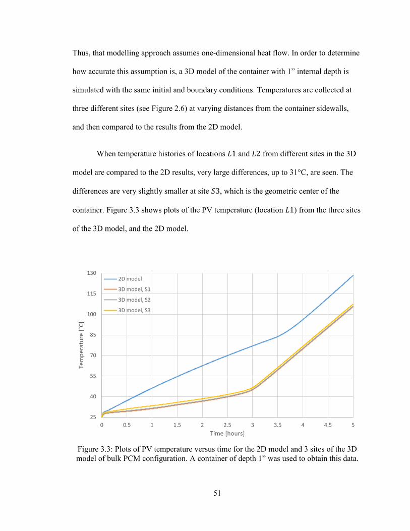
Thus, that modelling approach assumes one-dimensional heat flow. In order to determine

how accurate this assumption is, a 3D model of the container with 1” internal depth is

simulated with the same initial and boundary conditions. Temperatures are collected at

three different sites (see Figure 2.6) at varying distances from the container sidewalls,

and then compared to the results from the 2D model.

When temperature histories of locations 𝐿1 and 𝐿2 from different sites in the 3D

model are compared to the 2D results, very large differences, up to 31°C, are seen. The

differences are very slightly smaller at site 𝑆3, which is the geometric center of the

container. Figure 3.3 shows plots of the PV temperature (location 𝐿1) from the three sites

of the 3D model, and the 2D model.

Figure 3.3: Plots of PV temperature versus time for the 2D model and 3 sites of the 3D

model of bulk PCM configuration. A container of depth 1” was used to obtain this data.

25

40

55

70

85

100

115

130

0 0.5 1 1.5 2 2.5 3 3.5 4 4.5 5

Tem

per

atu

re [

°C]

Time [hours]

2D model

3D model, S1

3D model, S2

3D model, S3

52

In Figure 3.3, the PV temperature rises with a much higher slope during PCM

melt in the 2D case because the incoming heat is accumulated within the top layers of

PCM. The same was expected of the 3D model, but a lower initial slope is seen. This is

because of the way the models are set up. While the 2D setup assumes an infinitely large

box, with the only contact between top and bottom through the PCM filling, the 3D setup

has the top and bottom walls of the container connected at the outer boundaries with the

aluminum sidewall. Due to aluminum’s high thermal conductivity, the sidewall

effectively provides a low resistance path for the heat to travel down from the incoming

flux at the top surface to the bottom surface.

This affects the way heat is distributed into the PCM, resulting in different shapes

of the temperature contours at full PCM melt time. The 2D case isotherms (see Figure

3.1) suggest that the bottom layer of PCM, next to location 𝐿2 will be the last to melt.

But, due to the sidewall connection between the top and bottom plates in the 3D case, the

PCM close to the halfway depth in the container is the last part to melt. This can be seen

in Figure 3.4.

Figure 3.4: Temperature contours of the 3D model of the bulk PCM container at PCM

saturation time. The difference in shape from the 2D model contours in Figure 3.1 point

to a different melt pattern.

PCM

Top

plate

Sidewall

Bottom

plate

53

A better agreement between the 2D and 3D models would be seen if the container

were made of a material with low thermal conductivity, such as HDPE. For the current

design of an aluminum container, the results of the 3D simulation are more reliable. The

3D simulation shows that with a container of internal depth of 1”, full PCM saturation

occurs after 3 hours and 6 minutes; the PV temperature at this time is 49°C.

The conclusion made from the 2D simulations about greater container depth

regulating PV temperature for longer still holds. Thus, for all the following

configurations investigated, the internal depth of the PCM container is fixed at 1”. Also,

as shown by the comparison between 2D and 3D geometries, connecting the top and

bottom plates of the container with a high thermal conductivity material is beneficial to

the temperature regulation system. Hence, straight aluminum fins in the container will be

explored next.

3.2 Container with Straight Fins

In order to distribute heat evenly into the PCM volume to lower PV temperature

during the melt phase of PCM, straight aluminum fins are added to the container. These

fins are attached to the top plate that is in contact with the PV panel.

3.2.1 Two-Dimensional Model

Three different cases of the finned container are modelled as 2D geometries. In

these cases, the length, width and spacing between fins are varied to study the effect on

PV temperature. In the reduced domain 2D geometry that utilizes symmetry, only one fin

is modelled at the center of the PCM block.

54

3.2.1.1 Case I

The length of the aluminum fins is varied between 0 mm (no fin; geometry is

identical to bulk PCM configuration) and 25.4 mm (fins connect top and bottom plates of

the container). Plots of PV temperature (location 𝐿1) for selected fin lengths are shown in

Figure 3.5.

Figure 3.5: PV temperature versus time for varying fin lengths obtained from the

2D model of finned container.

In the above graph, all plots start with a high initial slope, where the PCM close to

the PV heats up quickly. Once the PV (and the surrounding PCM) temperature reaches

27.6°C, the PCM layers begin to melt and the slopes decrease. Then, once all the PCM in

the block is saturated, the slopes shoot up again and are equal because the effects of latent

heat of the PCM are used up.

25

40

55

70

85

100

115

130

0 0.5 1 1.5 2 2.5 3 3.5 4 4.5 5

Tem

per

atu

re [

°C]

Time [hours]

No fin

4mm fin

10mm fin

16mm fin

20mm fin

23mm fin

25.4mm fin

55

While the PCM melts, the slopes are higher for shorter fins, and reach the final

knee at higher PV temperatures and longer times. Due to poor thermal conductivity of the

PCM, local PCM close to the PV saturates very quickly and gets superheated while the

PCM further down in the block gets only small amounts of heat. This is confirmed by

trends seen in plots of location 𝐿2, in Figure 3.6.

Figure 3.6: Plots of location 𝐿2 (inside bottom surface) versus time for varying fin

lengths.

For 0 mm fin, and other short fins, the bottom surface temperature plots have an

almost zero slope during PCM melt, shooting up immediately when they hit the melt

temperature of 29.6°C. This trend becomes less drastic and the initial slope increases as

the fin length is increased; the change in slope afterwards still exists, but

25

40

55

70

85

100

115

0 0.5 1 1.5 2 2.5 3 3.5 4 4.5 5

Tem

per

atu

re [

°C]

Time [hours]

No fin

4mm fin

10mm fin

16mm fin

20mm fin

23mm fin

25.4mm fin

56

happens gradually, and at a temperature above 29.6°C. The 1” fin design exhibits this

knee in the graph at around 43°C.

Figure 3.6 indicates that with increasing fin length, PCM at the bottom of the

container is not the last to saturate. For the longer fins, even when the 𝐿2 temperature

exceeds the melt range, incoming heat is still being used up to melt PCM elsewhere, and

thus no sudden spike is seen in the temperature plots at 29.6°C.

Temperature contours of geometries with different fin lengths at full PCM melt

are shown in Figure 3.7. As the fin length increases, the last part of PCM to saturate shifts

upwards from the bottom surface. For the 1” long fin, with connects top and bottom

aluminum plates, location 𝐿6 is where the melt process ends, making the temperature

distribution almost perfectly symmetric along the depth of the container.

Figure 3.7: Temperature contours at PCM saturation time for different fin lengths. Red

represents the hottest temperature, and blue represents the coldest temperature.

The more even distribution of heat in geometries with longer fins leads to lower

PV temperature throughout the simulation. One hour into the simulation, the difference in

PV temperatures (see Figure 3.5) between shortest and longest fins is 16°C. The greatest

temperature difference is 36°C at around 3 hours. At the end of simulation, the 25.4 mm

57

fin design has a PV temperature 26°C lower than the no fin (0 mm) design. A

combination of lower PV temperature and higher bottom surface temperature at all times

in the simulation indicates that with longer fins heat is being more effectively moved

away and used to melt PCM away from the PV surface. Shorter melt times and lower PV

temperatures are thus the trend seen in Figure 3.8.

Figure 3.8: PCM saturation time and corresponding PV temperature for different fin

lengths.

With increasing fin length, PCM saturation time also decreases due to a

combination of two effects. First, a greater part of the incoming heat is carried down into

the PCM block at all times by a longer fin. This brings the PCM closer to saturation at an

earlier time. Second, the area of PCM in the 2D block decreases, which decreases the

amount of thermal mass that can absorb heat without changing temperature.

An interesting result is seen for the longest fins, where the melt time goes up

again, and significantly for the 1” long fin that connects top and bottom plates of the

25

35

45

55

65

75

85

2:45:00

2:52:30

3:00:00

3:07:30

3:15:00

3:22:30

3:30:00

Temp

erature [°C

]Tim

e [h

:mm

:ss]

Fin Length [mm]

Full PCM melt

PV temperature

58

container. This is explained by considering how the incoming heat is distributed

throughout the geometry. In designs with short fins, heat flow is almost perfectly one-

dimensional. The bottom part of the PCM is always the coolest region of the block. The

bottom plate of the aluminum container, which is only in contact with PCM also stays at

the same temperature as the PCM next to it. But, for fins of length 1”, the bottom plate is

thermally connected to the top plate through the fin. The fin provides a low resistance

path for heat to travel down the PCM block, as noted earlier. Thus, the bottom plate

reaches high temperatures much sooner while the PCM melts. This is an effective use of

the heat capacity of the aluminum bottom plate that allows for longer PCM saturation

time.

3.2.1.2 Case II

In this case a fin of length 13 mm is modelled with a combination of varying

width and spacing values. Since there are 16 designs investigated, results are presented

by grouping them into constant fin width and constant fin spacing plots.

Constant spacing graphs are presented first. Each graph contains plots for four fin

widths, ranging from 1 mm to 3.175 mm. Figure 3.9 shows plots of location 𝐿1 for

different fin widths at constant spacing of 1.5”. Plot of every fin width on this graph

shows a common characteristic of the temperature rising fast initially, until it reaches

around 27.6°C and the PCM layer close to the PV panel starts to melt. Then the slope

decreases, as the latent heat is used up in changing phase. A second knee around halfway

through the simulation is seen, where the slope increases again and PV temperatures rise

59

faster. This can be explained by all the PCM in the block completely melting, which

leads to all the incoming heat now being used for raising the temperature.

Figure 3.9: 𝐿1 temperature plots for finned container Case II. The fin length is held

constant at 13 mm. This graph shows four fin widths arranged with the same spacing of

1.5”.

PV temperature plots for Case II for other constant spacing values are shown in

Appendix A. At the end of the simulation time of 5 hours, the smaller spacing plots end

with lower PV panel temperatures. As spacing is increased, the PV surface ends up

hotter. The final PV temperature falls between 114°C and 118°C for different fin widths

with 0.5” spacing, and around 121°C for different fin widths with 2” spacing. This result

shows that fins arranged close together are more effective at spreading the heat sideways;

larger spacing designs are unable to do this because the low thermal conductivity of a

larger amount of PCM on both sides of the fin hinders heat flow.

25

40

55

70

85

100

115

130

0 0.5 1 1.5 2 2.5 3 3.5 4 4.5 5

Tem

per

atu

re [

°C]

Time [hours]

spacing 1.5" — width 1mm

spacing 1.5" — width 1.5mm



60

Figure 3.10 shows a graph with temperature plots of location 𝐿5 for this case with

a constant fin spacing of 1.5”. Graphs for other spacing values are shown in Appendix A.

Fin widths are varied for different plots. All plots begin with a low slope, even though the

PCM is not in the melt temperature range. This indicates that a very low amount of heat

is carried over from the top part of the block to this bottom layer of PCM.

After this, once the temperature reaches around 27.6°C, the graphs become almost

flat for a long time until the entire block of PCM melts. Once temperature at this location

reaches 29.6°C, which marks the end of phase change, there is a sudden rise in slopes.

This behavior indicates that PCM at location 𝐿5 is the last to saturate, and is confirmed

from the temperature contours at full PCM melt.


constant at 13 mm. This graph shows four fin widths arranged with the same spacing of

1.5”.

25

40

55

70

85

100

115

0 0.5 1 1.5 2 2.5 3 3.5 4 4.5 5

Tem

per

atu

re [

°C]

Time [hours]





61

Figures 3.9 and 3.10, and other plots in Appendix A, show that for the same fin

length of 13 mm and constant spacing, varying fin width has only a minor impact on the

temperature plots. The shapes of the plots are almost identical, and they all lie on top of

each other.

Results for Case II are now presented grouped together in constant fin width

graphs. Each graph contains four plots, for fin spacing ranging from 0.5” to 2”. Figure

3.11 shows PV temperature plots for a constant fin width of 1.5 mm. The plots show that

as the space between fins is increased, temperature of 𝐿1 rises with a higher slope during

PCM melt. Final temperature is also higher for larger spacing designs. Similar graphs for

other constant fin widths are shown in Appendix B.


constant at 13 mm. This graph shows fins of width 1.5 mm arranged with four different

values of fin spacing.

25

40

55

70

85

100

115

130

0 0.5 1 1.5 2 2.5 3 3.5 4 4.5 5

Tem

per

atu

re [

°C]

Time [hours]


spacing 1" — width 1.5mm



62

Plots of location 𝐿5, which is the last part of the PCM to melt, are shown in

Figure 3.12. It is seen that the location of the last knee in the graph, which marks PCM

saturation, varies with fin spacing – the smaller spacing designs have this knee at an

earlier location than the others since more heat reaches down with fins stacked close

together. Similar graphs for other constant fin widths are shown in Appendix B. These

graphs show that when fin width is increased, the location of this knee moves gradually

to an earlier time. This shows that wider fins are marginally better at carrying more heat

to the bottom part of the PCM container.


constant at 13 mm. This graph shows fins of width 1.5 mm arranged with four different

values of fin spacing.

25

40

55

70

85

100

115

0 0.5 1 1.5 2 2.5 3 3.5 4 4.5 5

Tem

per

atu

re [

°C]

Time [hours]





63

3.2.1.3 Case III

A fin of length 25.4 mm is modelled with a combination of varying width and

spacing values. This fin connects the top and bottom plates of the container. Since there

are 16 designs investigated, results are presented by grouping them into constant fin

width and constant fin spacing plots.

Constant spacing plots are presented below. Figure 3.13 shows plots of PV

temperature (location 𝐿1) for a constant spacing of 1.5” and varying fin width. Graphs for

other constant spacing values are provided in Appendix C. In every fin spacing graph, the

PV temperature with wider fins starts cooler, but around 2 hours into the simulation

becomes hotter than designs with thinner fins. The slopes of the plots then increase when

the PCM fully melts.

Figure 3.13: 𝐿1 temperature plots for finned container Case III. The fin length is held

constant at 25.4 mm. This graph shows four fin widths arranged with the same spacing of

1.5”.

25

40

55

70

85

100

115

0 0.5 1 1.5 2 2.5 3 3.5 4 4.5 5

Tem

per

atu

re [

°C]

Time [hours]





64

At the end of the simulation at 5 hours, the 3.175 mm fin always ends up with the

hottest PV temperature due to reduced PCM in the block since a greater area is covered

by a thicker aluminum fin. This difference in final 𝐿1 temperatures is more pronounced

in the smallest fin spacing (0.5”) graph, where the widest fin design ends 10°C higher

than the thinnest fin. The difference becomes smaller and drops to 2°C as the fin spacing

increases to 2”. This happens because in the 2D geometry, changing fin width in

larger spacing designs has a smaller effect on the ratio of PCM area to aluminum area.

When compared to the equivalent graphs for Case II (see Figure 3.9 and

Appendix A), it is notable that the knee at full melt occurs at much higher PV

temperatures for the 13 mm long fin plots than the 1” long fin. In Case II, the lowest knee

occurs at 57°C and the highest knee occurs at 71°C. In Case III, the lowest knee is seen at

a PV temperature of 33°C, while the highest knee is at 47°C. Thus, for all variations of

fin spacing and fin width, the 13mm long fin does a worse job of taking the heat away

from the PV panel. This results in a much higher slope of 𝐿1 temperature plots before the

knee when compared to plots of 1” long fin.

Since the 1” fin of Case III connects top and bottom plates of the container, the

last part of PCM to saturate is at location 𝐿6. Thus, temperature plots of this location,

shown in Figure 3.14 and Appendix C, have the characteristic zero slope during phase

change and a sharp knee at PCM saturation. Compared to the equivalent graphs of the last

location to melt for Case II (see Figure 3.10 and Appendix A), there are differences in

how the plots start. All Case II plots begin with a low slope, even though the PCM is not

in the melt temperature range, indicating that very little heat reaches 𝐿5. In Case III, with

65

a longer fin, the plot slopes are high initially, and then decrease when the local PCM

enters the melt phase. This indicates that comparatively more heat reaches the coolest

part of the PCM block.

Figure 3.14: 𝐿6 temperature plots for finned container Case III. The fin length is held

constant at 25.4 mm. This graph shows four fin widths arranged with the same spacing of

1.5”.

Temperature plots of locations 𝐿1 and 𝐿6 for Case III, grouped together in

constant fin width graphs are shown in Appendix D. Trends similar to Case II are seen.

Results from all designs in Cases II and III of finned PCM container are now

presented together. The differences in PCM saturation time and PV temperature at this

time for all fin spacing and width combinations are shown in Figure 3.15.

25

40

55

70

85

100

115

0 0.5 1 1.5 2 2.5 3 3.5 4 4.5 5

Tem

per

atu

re [

°C]

Time [hours]





66

Figure 3.15: Plots of PCM saturation time and PV temperature at this time for varying fin

width and spacing in Cases II and III.

For the same fin spacing, melt times drop slightly with increasing fin width due to

a slightly reduced PCM area. This effect is more pronounced in smaller spacing designs

because the PCM reduction has a greater effect on the area ratio of PCM to aluminum

than in larger spacing designs. As fin spacing is increased, the area ratio of PCM

increases, and so does the time to saturate.

Since 13mm long fins of Case II do a worse job of moving the heat away from the

PV surface, it takes longer to saturate all the PCM in the block. A greater part of the

incoming heat is thus used up in increasing the PV temperature. The combination of these

two effects – locally accumulated heat and longer time to melt – leads to Case II designs

25

30

35

40

45

50

55

60

65

70

75

2:00:00

2:15:00

2:30:00

2:45:00

3:00:00

3:15:00Tem

peratu

re [°C]

Tim

e [h

:mm

:ss]

Fin sapcing [inches] — fin width [mm]

Case II PCM saturation Case III PCM saturation

Case II PV temperature Case III PV temperature

67

having a much higher PV temperature at full melt. For every combination of fin spacing

and width, Case II PV temperature at saturation is around 22°C hotter than Case III.

As the fin width is increased, the PV temperature at melt is slightly lower because

wider fins are marginally better at carrying heat away from the PV surface. When spacing

is increased, the PV temperature at full melt goes up because the incoming heat has to

travel through a wider area of low thermal conductivity PCM before saturation occurs.

Overall, for both Cases II and III, changing the fin width only has a minor effect

on the regulation of PV temperature. For 13mm long fins and constant spacing,

increasing fin width only decreases PV temperature at saturation by around 2.5°C. For

25.4mm long fins, this decrease is even smaller, at around 1.5°C. The accompanying

reduction in PCM saturation time with increasing fin width makes thinner fins more

suitable. Changing the spacing between fins has a more significant effect on the results –

with increasing spacing the PV temperatures rise up.

Among all the designs modelled, Case II (fin length 25.4 mm) with a fin spacing

of 0.5” has the lowest PV temperatures at full melt. With this spacing, PV temperature at

saturation decreases by 1.5°C when fin width is increased from 1 mm to 3.175 mm. But,

this also decreases PCM saturation time by 32 minutes. Hence, fins of length 25.4 mm,

width 1mm and spaced 0.5” apart are deemed most effective for use in the temperature

regulation system.

68

3.2.2 Three-Dimensional Model

Two geometries of the finned container configuration are modelled in three

dimensions and the results compared to their respective equivalent 2D models. In both

cases, the fins have a length of 1”, and so the PCM is divided into separate blocks.

3.2.2.1 Case I

In this case, the fin width is 1 mm and fin spacing is 0.5”. The temperature results

from locations 𝐿1 through 𝐿6, collected at each of the 6 sites, 𝑆1 through 𝑆6 (see Figure

2.10), are plotted and compared graphically to results from the analogous 2D simulation.

All throughout the 5 hours of simulation time the plots match closely. For every location,

temperature plots from the 2D geometry are always slightly higher than plots from the 3D

geometry. Figure 3.16 shows this trend in plots of location 𝐿1, where the 2D model ends

with a slightly higher PV temperature by 5°C. This happens because the 3D model has

some extra thermal mass of the container sidewalls that were not modeled in the 2D

geometry. The temperature of these walls is also raised long with the PCM in the

container, making them heat storage components.

69

Figure 3.16: Temperature plots of location 𝐿1 obtained from the 2D model, and six sites

of the 3D model.

Plots of all six sites from the 3D model are almost identical, indicating that heat is

distributed evenly throughout the PCM container, and hence there is not much difference

in where the data is collected inside the container. Thus, the use of symmetry to reduce

the model to a 2D geometry is justified.

There is a slight variation seen in PCM saturation times between the six sites of

the 3D model. In the PCM block adjacent to the container sidewall, PCM saturates first at

site 𝑆1, then 𝑆2, and last at 𝑆3. Because site 𝑆1 is close to two container walls, the

thicker sidewalls act as thick fins and bring slightly more heat from the top plate into the

PCM. This causes PCM at this site to melt sooner. The effect of the second sidewall

diminishes as the sites get closer to the middle of the PCM container. A similar trend is

25

40

55

70

85

100

115

0 0.5 1 1.5 2 2.5 3 3.5 4 4.5 5

Tem

per

atu

re [

°C]

Time [hours]

2D model

3D model, S1

3D model, S2

3D model, S3

3D model, S4

3D model, S5

3D model, S6

70

seen in the PCM block in the center of the container, where PCM at site 𝑆4 melts first,

then 𝑆5, and 𝑆6 last.

When melt times are compared between the two PCM blocks of interest, it is seen

that PCM in the block adjacent to the sidewall saturates at a slightly later time. This

occurs this due to the sidewalls of PCM surrounding it on three sides, which store a part

of the incoming heat which would have otherwise gone into melting the PCM.

Table 3.2 compares the 2D and 3D models for PCM saturation time and PV

temperature at this time. Very small differences are seen, as quantified by the percentage

difference in PV temperatures at full melt.

Table 3.2: Results from Case I of 3D models for finned PCM configuration compared to

equivalent 2D model.

2D model 3D model, S3 3D model, S6

PCM saturation time [ℎℎ: 𝑚𝑚] 02h:51m 02h:56m 02h:52m

PV temperature @ PCM saturation [°𝐶] 34.0 35.5 33.7

Percent Difference 4.1% -1.1%

3.2.2.2 Case II

In this case, fins of width 3.175 mm are arranged with a spacing of 1”. Graphical

comparison of temperature data from six locations at sites S1 through S6 with the 2D

model results shows minimal differences. Between the six sites of the 3D model, trends

similar to Case I are seen.

71

Table 3.3 presents results of PCM saturation time and PV temperature at this

time. The results of the 3D model are compared to that of the equivalent 2D model, and a

good agreement between the two modelling approaches is seen.

Table 3.3: Results from Case II of 3D models for finned PCM configuration compared to

equivalent 2D model.

2D model 3D model, S3 3D model, S6



Percent Difference 2.9% -1.0%

Overall, results from the finned PCM container show a marked improvement over

the bulk PCM configuration. Fin length has the most significant impact on the regulation

of PV temperature, with the longest fin providing lowest PV temperatures. With this fin

length, PCM saturation time also increases, which is a break from the trend of shorter

melt times with increasing length. Fin spacing is next in importance, since changing it

affects the farthest any point in PCM is from a high thermal conductivity heat flow path.

Fin width has only a minimal impact on PV temperature. In fact, increasing fin width

shortens saturation time, which is a negative effect on the temperature regulation system.

Results suggest that long, thin fins with small spacing are most suitable for mitigating the

effects of low thermal conductivity of PCM. A honeycomb structure, which matches

these criteria, is investigated and results presented in the next section.

72

3.3 Container with Honeycomb Core Fin

An aluminum honeycomb core is modelled in the PCM container. The depth of

the honeycomb is 1”, so it connects the top and bottom plates of the container. The PCM

is also divided into cells, and temperature is monitored at four of the cells (see Figure

2.16). Results are compared to Case I and Case II of the 3D model of finned container

configuration. Case I has fins of length 1”, width 1mm and spacing 0.5”. Case I has fins

of length 1”, width 3.175mm, and spacing 1”.

3.3.1 Case I

In Case I, the cell size of the honeycomb is 1”. Temperature contours of all four

PCM cells were plotted at full PCM melt, and were found to be similar. Figure 3.17

shows the temperature contours for cell 𝑇𝐿. It can be seen that the honeycomb effectively

carries heat away from the PV surface and distributes it evenly to the enclosed PCM cells

because of the near symmetry in temperatures seen between the top and bottom halves of

the model.

73

Figure 3.17: Temperature contours at full melt for honeycomb configuration Case I. Only

the PCM cell is shown.

For each PCM cell, the last part of the PCM to melt is verified to be at or very

close to the centroid, whose temperature is monitored as it is analogous to location 𝐿6 in

Figure 2.11. This is also seen in the temperature plots of this location for all PCM cells,

where the slope remains flat in the melt temperature range of the PCM, and once

saturated, immediately increases. Figure 3.18 shows these plots of location 𝐿6 for the

four PCM cells of the honeycomb configuration, and two 3D finned container models.

74


configuration, and four cells of the honeycomb configuration Case I.

The figure above shows that the two finned designs melt very close to each other.

All PCM cells in the honeycomb configuration reach saturation last, and also have the

lowest final PCM temperature. The difference in final temperatures of the PCM at 𝐿6 is

around 10°C.

𝐿1 temperature from the same configurations is plotted in Figure 3.19.

Throughout the simulation time, the PV panel is almost always maintained at lower

temperatures by using the honeycomb core rather than straight fins in the PCM container.

At the end of simulation, the honeycomb configuration PV temperature is 92°C. This

value is 5°C lower than the finned container Case I, and 9°C lower than the finned

container Case II.

25

40

55

70

85

100

0 0.5 1 1.5 2 2.5 3 3.5 4 4.5 5

Tem

per

atu

re [

°C]

Time [hours]

3D finned Case I

3D finned Case II

Honeycomb Case I, TR

Honeycomb Case I, TL

Honeycomb Case I, BR

Honeycomb Case I, BL

75


configuration, and four cells of the honeycomb configuration Case I.

A comparison of PCM saturation time and the PV temperature at this time for the

two finned 3D designs and the honeycomb Case I is shown in Table 3.4. It is seen that

finned container Case I melts soonest, and the PV temperature at this time is the lowest.

Finned container Case II saturates next. Even though this design melts slightly later, the

gains in melt time come with a higher PV temperature at full PCM melt. The honeycomb

PCM cells have the longest saturation time of 3h:17m. This due to the extra volume of

PCM in the container made possible by the very small thickness of the honeycomb of 0.2

mm. This melt time is an improvement of 21 minutes and 16 minutes over finned

container Cases I and II, respectively. At full melt, the PV temperature is 40.9°C, which

is higher than that of finned container Case I. But, it is seen from Figure 3.19 that at the

same time, that design has reached a PV temperature of 46.1°C.

25

40

55

70

85

100

115

0 0.5 1 1.5 2 2.5 3 3.5 4 4.5 5

Tem

per

atu

re [

°C]

Time [hours]

3D finned Case I

3D finned Case II

Honeycomb Case I, TR

Honeycomb Case I, TL

Honeycomb Case I, BR

Honeycomb Case I, BL

76


honeycomb configuration Case I.

3D finned

Case I

3D finned

Case II

Honeycomb

Case I



3.3.2 Case II

In Case II, the cell size of the honeycomb is 0.5”. This case is modelled to see if a

smaller honeycomb cell size (effectively reducing fin spacing) has the same significant

effect on PV temperature as it did with straight fins. Temperature contours of the

monitored PCM cells are again very similar, with an even heat distribution seen. The last

part of every PCM cell to saturate is again at location 𝐿6.

Figure 3.20 shows 𝐿1 temperature plots from two 3D finned container designs

and honeycomb Case II. All plots from the honeycomb configuration fall on top of each

other, suggesting that the location of the PCM cell in the container does not matter.

Throughout the simulation, the honeycomb configuration has the lowest PV

temperatures. At the end of the simulation, the PV temperature for Case II of honeycomb

configuration is 93°C. This is 4°C lower than the first finned container Case I, and 8°C

lower than the finned container Case II.

77


configuration, and four cells of the honeycomb configuration Case II.

Table 3.5 shows PCM saturation time and PV temperature at this time for

honeycomb configuration Case II. When compared to the two finned designs, this design

gives a melt time improvement of 6 minutes over Case I, and 2 minutes over Case II.

These gains are smaller than were seen in honeycomb configuration Case I. A larger

improvement is seen in PV temperature at PCM saturation. The PV temperature at melt is

lowered by 1.5°C and 8°C when compared to finned container Cases I and II,

respectively.

25

40

55

70

85

100

115

0 0.5 1 1.5 2 2.5 3 3.5 4 4.5 5

Tem

per

atu

re [

°C]

Time [hours]

3D finned Case I

3D finned Case II

Honeycomb Case II, TR

Honeycomb Case II, TL

Honeycomb Case II, BR

Honeycomb Case II, BL

78


honeycomb configuration Case II.

3D finned

Case I

3D finned

Case II

Honeycomb

Case II



Comparing the two honeycomb configuration cases, all PCM in Case II saturates

15 minutes sooner than in Case I. This is because smaller sized honeycomb cells reduce

the amount of PCM in the container. Shorter melt time of Case II is also accompanied by

a 6.8°C lower PV temperature at full melt.

3.4 Encapsulated PCM

In this configuration, spherical HDPE pellets containing PCM are placed inside

the container. The remaining volume of the container is filled with water. Temperature

contours of the quarter model at PCM saturation, shown in Figure 3.21, show that the

center of the container has highest temperatures and longest melt time. Thus, temperature

data was only collected at this site.

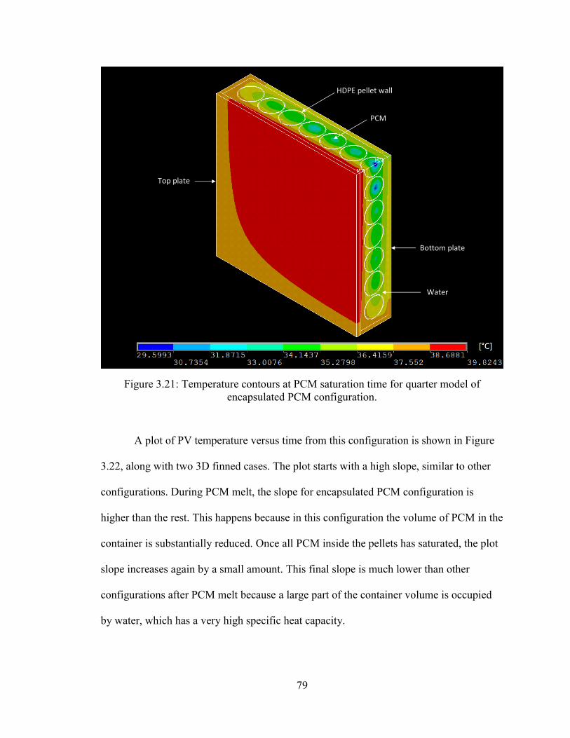
79

Figure 3.21: Temperature contours at PCM saturation time for quarter model of

encapsulated PCM configuration.

A plot of PV temperature versus time from this configuration is shown in Figure

3.22, along with two 3D finned cases. The plot starts with a high slope, similar to other

configurations. During PCM melt, the slope for encapsulated PCM configuration is

higher than the rest. This happens because in this configuration the volume of PCM in the

container is substantially reduced. Once all PCM inside the pellets has saturated, the plot

slope increases again by a small amount. This final slope is much lower than other

configurations after PCM melt because a large part of the container volume is occupied

by water, which has a very high specific heat capacity.

Top plate

Bottom plate

HDPE pellet wall

PCM

Water

80

Figure 3.22: Plot of PV temperature versus time for encapsulated PCM configuration.

PCM in the encapsulated configuration saturates after 1 hour and 22 minutes. The

PV temperature at this time is 39.8°C. Almost every other container configuration

modelled has a lower PV temperature at this time.

3.5 Cost Comparison

Plots of PV temperature versus time for a few selected configurations are

compiled in Figure 3.23.

25

40

55

70

85

100

115

0 0.5 1 1.5 2 2.5 3 3.5 4 4.5 5

Tem

per

atu

re [

°C]

Time [hours]

3D finned Case I

3D finned Case II

Encapsulated

81

Figure 3.23: PV temperature plots for different PCM container configurations.

A wide variation in saturation times and PV temperatures is seen. To compare the

performance of the configurations directly against each other, the cost of each

configuration is computed using Equation 2.3. The results are shown in Table 3.6.

Table 3.6: Costs for various container configurations.

PCM Container Configuration Cost, 𝑱 [°𝐶 ∙ 𝑠]

Bulk 3D 839,003

Finned 3D Case I 359,950

Finned 3D Case II 409,631

Honeycomb Case I 334,469

Honeycomb Case II 326,978

Encapsulated 659,470

25

40

55

70

85

100

115

130

0 0.5 1 1.5 2 2.5 3 3.5 4 4.5 5

Tem

per

atu

re [

°C]

Time [hours]

Bulk 3D

Finned 3D Case I

Finned 3D Case II

Honeycomb Case I

Honeycomb Case II

Encapsulated

82

Table 3.6 shows that when compared for a five-hour time period, a PCM

container with a honeycomb fin with 0.5” cell size is most effective at maintaining low

PV panel temperature over a long duration. Very close performance is also seen from

honeycomb of 1” cell size, and a straight fins of length 1”, width 1 mm, and spacing 0.5”.

Figure 3.24: Graphical comparison of performance metrics.

(better) →

(better) →

← (better)

83

Figure 3.24 shows all three performance metrics – PCM saturation time, PV

temperature at saturation, and cost – compared graphically. Configurations with longer

saturation times, lower PV temperatures at saturation and lower cost over the 5-hour

simulation time are considered better suited for temperature regulation.

84

Chapter IV

Conclusions and Future Work

PV panels are a commonly used to convert solar energy to clean electricity. But,

their energy conversion efficiency drops with an increase in panel temperature with

exposure to insolation. This thesis explores a PCM-based passive temperature regulation

system for PV panels. The PCM is placed into a container attached to the back surface of

the panel, and absorbs incoming heat at a constant temperature while changing phase.

Four configurations of PCM inside the aluminum container are explored.

In the first configuration, bulk PCM fills up the entire interior volume of the

container. With three different depths of the container modelled (0.33”, 0.5” and 1’), it is

seen that a deeper container regulates the PV temperature for a longer time. However, the

rise in PV temperature during the melt phase of PCM occurs at the same rate for each

depth of container. This suggests that the extra thermal mass of PCM in deeper containers

is not being effectively utilized to regulate temperature. And, in the absence of any heat

transfer mechanism to remove heat from the PCM in the container, PV temperature still

reaches high values.

A three-dimensional model of the bulk PCM container is also created, and results

compared to the 2D model. Results show that the sidewalls of the container are able to

remove a part of the incoming heat to the bottom layers of PCM, thus decreasing PV

temperature and PCM saturation time. Since this container design has no aluminum fin

85

connecting the top and bottom plates, the 2D model under predicts the performance of the

temperature regulation system.

With the knowledge that addition of aluminum to the PCM container improves

performance, straight aluminum fins are added to a container of 1” internal depth in order

to promote heat transfer into the PCM away from the PV panel. The effects of varying fin

length, width and spacing are investigated. Results show that with an increase in fin

length, a larger part of the incoming heat is used as latent heat to melt PCM away from

the PV panel, and hence, PV temperature is lowered. This is accompanied by a slight

drop in saturation time. Fin width and spacing are then varied for two selected fin lengths

– 13 mm and 25.4 mm. Results from both fin lengths show that wider fins are only

marginally better at removing heat from the PV panel. Reduction in fin spacing as a more

significant impact on PV temperature. Any increase in fin length or width, or a decrease

in spacing, causes PCM saturation time to drop because of the reduced volume of PCM in

the container. A container design with fins of length 1”, width 1 mm, and spacing 0.5”

offers a good combination of relatively high saturation time of 2 hours and 51 minutes,

and one of the lowest PV temperatures at full melt of 34°C.

Three-dimensional models two finned PCM container configurations are created.

In both these designs, there are 1” long fins that connect the top and bottom aluminum

plates. The results from 2D models of finned container still match very well with the 3D

models. Only a small difference in melt times is seen because the added thermal mass of

the container sidewalls is not present in the 2D models.

86

Since long, thin fins stacked close together are found best at maintaining low PV

temperatures, an aluminum honeycomb core is used as a fin in the next configuration.

The honeycomb has a depth of 1” to connect the top and bottom container plates, and two

cell sizes are modelled: 0.5” and 1”. Both cases show a slight improvement in melt times

over the most effective finned container design. PV temperatures at full melt are also

among the lowest, at 40.9°C for 1” cells, and 34.1°C for 0.5” cells.

The encapsulated PCM configuration tries to overcome the problems of

packaging and low thermal conductivity of the PCM. The PCM is in spherical pellets

which provide a larger surface area for heat exchange. Water is used as a medium to draw

heat from the container walls and bring it to the pellets. Results show a very short

saturation time due to the substantially reduced PCM volume. The PV temperature is also

higher than finned or honeycomb configurations throughout the simulation. These

drawbacks of the encapsulated PCM configuration could be mitigated by altering the size

of the pellets so that a larger volume of PCM can be carried inside the container.

Values of the developed cost function are computed for a few selected

configurations and compared to gauge their performance. The minimum cost among

these configurations is attained when using an aluminum honeycomb core of cell size

0.5” as a fin in the PCM container. Other configurations with similarly low costs are

honeycomb core fin of 1” cell size, and straight fins of length 1”, width 1 mm and

spacing 0.5”.

In this purely numerical analysis, perfect thermal contact is assumed between the

container plates and the straight or honeycomb core fins. However, the honeycomb core

87

has a very small foil thickness, and with realistic manufacturing considerations, it would

be very difficult to attach this to the to the container walls. Thus, good thermal contact

might not be achieved. It would be easier to manufacture a PCM container with straight

aluminum fins attached to the walls inside it. Also, when this temperature regulation

system is attached to a PV panel, it would be expected to work throughout the day. Thus,

an active heat exchanger cooling tube would pass through the container to re-solidify the

PCM upon saturation. Routing this tube would be much easier with straight fins than

with a honeycomb container. Thus, in a realistic manufacturing solution, a PCM

container with long, narrow, closely spaced straight fins would be the best option.

The results obtained from numerical simulations of various configurations show

that a PCM based system is an effective way of regulating PV panel temperature. More

work can be done to verify this claim. The numerical setup needs to be validated with

data from controlled laboratory experiments which mimic the geometry, heating load and

boundary conditions of the simulated model.

A different modelling approach for the PCM, called the enthalpy-porosity

method, can be used. This method tracks the position of the melt front of the PCM, and

captures convection effects in the melted regions.

Similarly, a CFD solver can be used to model the convection in the water inside

the container of the encapsulated configuration. This would promote the removal of heat

from the PV surface into the PCM pellets, and could result in lower PV temperature at

PCM saturation time.

88

The simulations set up for this work assumed a constant heat flux coming into the

adiabatic PCM container. This would not be the case in reality. To assess the

performance for varying outdoor conditions, the numerical experiments need to be set up

with varying values of the heating load and convective boundary conditions. Thermal

properties of the PV panel can also be factored in to affect how much solar insolation

turns to heat and reaches the PCM container.

After the above listed more detailed analyses are performed on the PCM container

configurations, the results can be used to select the most effective passive temperature

regulation system for PV panels that would limit the drop in electrical efficiency.

89

Appendix A

Figure A.1: 𝐿1 temperature plots for finned container Case II. Four fin widths arranged

with a spacing of 0.5” are shown.


with a spacing of 1” are shown.

25

40

55

70

85

100

115

130

0 0.5 1 1.5 2 2.5 3 3.5 4 4.5 5

Tem

per

atu

re [

°C]

Time [hours]





25

40

55

70

85

100

115

130

0 0.5 1 1.5 2 2.5 3 3.5 4 4.5 5

Tem

per

atu

re [

°C]

Time [hours]

spacing 1" — width 1mm




90





25

40

55

70

85

100

115

130

0 0.5 1 1.5 2 2.5 3 3.5 4 4.5 5

Tem

per

atu

re [

°C]

Time [hours]

sapcing 2" — width 1mm




25

40

55

70

85

100

115

0 0.5 1 1.5 2 2.5 3 3.5 4 4.5 5

Tem

per

atu

re [

°C]

Time [hours]





91





25

40

55

70

85

100

115

0 0.5 1 1.5 2 2.5 3 3.5 4 4.5 5

Tem

per

atu

re [

°C]

Time [hours]





25

40

55

70

85

100

115

0 0.5 1 1.5 2 2.5 3 3.5 4 4.5 5

Tem

per

atu

re [

°C]

Time [hours]





92

Appendix B

Figure B.1: 𝐿1 temperature plots for finned container Case II. This graph shows fins of

width 1 mm arranged with four different values of fin spacing.



25

40

55

70

85

100

115

130

0 0.5 1 1.5 2 2.5 3 3.5 4 4.5 5

Tem

per

atu

re [

°C]

Time [hours]





25

40

55

70

85

100

115

130

0 0.5 1 1.5 2 2.5 3 3.5 4 4.5 5

Tem

per

atu

re [

°C]

Time [hours]



sapcing 1.5" — width 2mm


93


width 3.175 mm arranged with four different values of fin spacing.



25

40

55

70

85

100

115

130

0 0.5 1 1.5 2 2.5 3 3.5 4 4.5 5

Tem

per

atu

re [

°C]

Time [hours]





25

40

55

70

85

100

115

0 0.5 1 1.5 2 2.5 3 3.5 4 4.5 5

Tem

per

atu

re [

°C]

Time [hours]





94





25

40

55

70

85

100

115

0 0.5 1 1.5 2 2.5 3 3.5 4 4.5 5

Tem

per

atu

re [

°C]

Time [hours]



sapcing 1.5" — width 2mm


25

40

55

70

85

100

115

0 0.5 1 1.5 2 2.5 3 3.5 4 4.5 5

Tem

per

atu

re [

°C]

Time [hours]





95

Appendix C

Figure C.1: 𝐿1 temperature plots for finned container Case III. Four fin widths arranged




25

40

55

70

85

100

115

0 0.5 1 1.5 2 2.5 3 3.5 4 4.5 5

Tem

per

atu

re [

°C]

Time [hours]





25

40

55

70

85

100

115

0 0.5 1 1.5 2 2.5 3 3.5 4 4.5 5

Tem

per

atu

re [

°C]

Time [hours]





96





25

40

55

70

85

100

115

0 0.5 1 1.5 2 2.5 3 3.5 4 4.5 5

Tem

per

atu

re [

°C]

Time [hours]





25

40

55

70

85

100

115

0 0.5 1 1.5 2 2.5 3 3.5 4 4.5 5

Tem

per

atu

re [

°C]

Time [hours]





97





25

40

55

70

85

100

115

0 0.5 1 1.5 2 2.5 3 3.5 4 4.5 5

Tem

per

atu

re [

°C]

Time [hours]





25

40

55

70

85

100

115

0 0.5 1 1.5 2 2.5 3 3.5 4 4.5 5

Tem

per

atu

re [

°C]

Time [hours]





98

Appendix D

Figure D.1: 𝐿1 temperature plots for finned container Case III. This graph shows fins of




25

40

55

70

85

100

115

0 0.5 1 1.5 2 2.5 3 3.5 4 4.5 5

Tem

per

atu

re [

°C]

Time [hours]





25

40

55

70

85

100

115

0 0.5 1 1.5 2 2.5 3 3.5 4 4.5 5

Tem

per

atu

re [

°C]

Time [hours]





99





25

40

55

70

85

100

115

0 0.5 1 1.5 2 2.5 3 3.5 4 4.5 5

Tem

per

atu

re [

°C]

Time [hours]





25

40

55

70

85

100

115

0 0.5 1 1.5 2 2.5 3 3.5 4 4.5 5

Tem

per

atu

re [

°C]

Time [hours]





100





25

40

55

70

85

100

115

0 0.5 1 1.5 2 2.5 3 3.5 4 4.5 5

Tem

per

atu

re [

°C]

Time [hours]





25

40

55

70

85

100

115

0 0.5 1 1.5 2 2.5 3 3.5 4 4.5 5

Tem

per

atu

re [

°C]

Time [hours]





101





25

40

55

70

85

100

115

0 0.5 1 1.5 2 2.5 3 3.5 4 4.5 5

Tem

per

atu

re [

°C]

Time [hours]





25

40

55

70

85

100

115

0 0.5 1 1.5 2 2.5 3 3.5 4 4.5 5

Tem

per

atu

re [

°C]

Time [s]





102

References

[1] U.S. Energy Information Administration, Net Generation by Energy Source: Total

(All Sectors), 2007-January 2017, in Electric Power Monthly. Retrieved March 21,

2017, from

https://www.eia.gov/electricity/monthly/epm_table_grapher.cfm?t=epmt_1_01

(2017).

[2] U.S. Energy Information Administration, U.S. electric generating capacity increase

in 2016 was largest net change since 2011. Retrieved March 21, 2017, from

https://www.eia.gov/todayinenergy/detail.php?id=30112# (2017).

[3] Weakliem, H., Redfield, D., “Temperature dependence of the optical properties of

silicon,” Journal of Applied Physics, 50, pp. 1491–1493 (1979).

[4] Krauter, S., “Actual optical and thermal performance of PV-modules,” in

“Proceedings of the 1st World Conference on Photovoltaic Energy Conversion,”

(1994).

[5] Radziemska, E., “The effect of temperature on the power drop in crystalline silicon

solar cells,” Renewable Energy, 28, pp. 1 – 12 (2003).

[6] Krauter, S., Araujo, R.G., Schroer, S., Hanitsch, R., Salih, M.J., Triebel, C., and

Lemoine, R., "Combined photovoltaic and solar thermal systems for facade

integration and building insulation," Solar Energy, 67, pp. 239 – 248 (1999).

103

[7] Chow, T., “A review on photovoltaic/thermal hybrid solar technology,” Applied

Energy, 87, pp. 365 – 379 (2010).

[8] Tyagi, V., Kaushik, S., and Tyagi, S., “Advancement in solar photovoltaic/thermal

(PV/T) hybrid collector technology,” Renewable and Sustainable Energy Reviews,

16, pp. 1383 – 1398 (2012).

[9] Ma, T., Yang, H., Zhang, Y., Lu, L., and Wang, X., “Using phase change materials in

photovoltaic systems for thermal regulation and electrical efficiency improvement: A

review and outlook,” Renewable and Sustainable Energy Reviews, 43, pp. 1273 –

1284 (2015).

[10] Häusler, T., and Rogaß, H., “Photovoltaic module with latent heat storage -

collector,” in “Proceedings of the 2nd World Conference and Exhibition on

Photovoltaic Solar Energy Conversion Vienna, Austria,” (1998).

[11] Häusler, T., and Rogaß, H., “Latent heat storage on photovoltaics,” in “16th

European Photovoltaic Solar Energy Conference Glasgow, UK,” (2000).

[12] Huang, M.J., Eames, P.C., and Norton, P., “Thermal regulation of building-

integrated photovoltaics using phase change materials,” International Journal of

Heat and Mass Transfer, 47, pp. 2715 – 2733 (2004).

[13] Huang, M., Eames, P., and Norton, B., “Phase change materials for limiting

temperature rise in building integrated photovoltaics,” Solar Energy, 80, pp. 1121 –

1130 (2006).

104

[14] Huang, M., Eames, P., and Norton, B., “Comparison of a small-scale 3D PCM

thermal control model with a validated 2D PCM thermal control model,” Solar

Energy Materials and Solar Cells, 90, pp. 1961 – 1972 (2006).

[15] Kosny, J., Biswas, K., Miller, W., Childs, P., and Kriner, S., “Sustainable retrofit of

residential roofs using metal roofing panels, thin-film photovoltaic laminates and

PCM heat sink technology,” Journal of Building Enclosure Design (2011).

[16] Kosny, J., Biswas, K., Miller, W., and Kriner, S., “Field thermal performance of

naturally ventilated solar roof with PCM heat sink,” Solar Energy, 86, pp. 2504 –

2514 (2012).

[17] Hasan, A., McCormack, S., Huang, M., and Norton, B., “Evaluation of phase change

materials for thermal regulation enhancement of building integrated photovoltaics,”

Solar Energy, 84, pp. 1601 – 1612 (2010).

[18] Huang, M., Eames, P., Norton, B., and Hewitt, N., “Natural convection in an

internally finned phase change material heat sink for the thermal management of

photovoltaics,” Solar Energy Materials and Solar Cells, 95, pp. 1598 – 1603 (2011).

[19] Biwole, P. H., Eclache, P., and Kuznik, F., “Phase-change materials to improve solar

panel’s performance,” Energy and Buildings, 62, pp. 59 – 67 (2013).

[20] Brano, V. L., Ciulla, G., Piacentino, A., and Cardona, F., “Finite difference thermal

model of a latent heat storage system coupled with a photovoltaic device:

Description and experimental validation,” Renewable Energy, 68, pp. 181 – 193

(2014).

105

[21] Park, J., Kim, T., and Leigh, S.-B., “Application of a phase-change material to

improve the electrical performance of vertical-building-added photovoltaics

considering the annual weather conditions,” Solar Energy, 105, pp. 561 – 574

(2014).

[22] Aelenei, L., Pereira, R., Gonçalves, H., and Athienitis, A., “Thermal performance of

a hybrid BIPV-PCM: Modeling, design and experimental investigation,” Energy

Procedia, 48, pp. 474 – 483 (2014).

[23] Aelenei, L., Pereira, R., Ferreira, A., Gonçalves, H., and Joyce, A., “Building

integrated photovoltaic system with integral thermal storage: A case study,” Energy

Procedia, 58, pp. 172 – 178 (2014).

[24] Maiti, S., Banerjee, S., Vyas, K., Patel, P., and Ghosh, P. K., “Self regulation of

photovoltaic module temperature in v-trough using a metal-wax composite phase

change matrix,” Solar Energy, 85, pp. 1805 – 1816 (2011).

[25] Hasan, A., McCormack, S., Huang, M., Sarwar, J., and Norton, B., “Increased

photovoltaic performance through temperature regulation by phase change materials:

Materials comparison in different climates,” Solar Energy, 115, pp. 264 – 276

(2015).

[26] Sharma, S., Tahir, A., Reddy, K., and Mallick, T. K., “Performance enhancement of

a building-integrated concentrating photovoltaic system using phase change

material,” Solar Energy Materials and Solar Cells, 149, pp. 29 – 39 (2016).

106

[27] Ho, C., Tanuwijava, A., and Lai, C.-M., “Thermal and electrical performance of a

BIPV integrated with a microencapsulated phase change material layer,” Energy and

Buildings, 50, pp. 331 – 338 (2012).

[28] Ho, C., Jou, B.-T., Lai, C.-M., and Huang, C.-Y., “Performance assessment of a

BIPV integrated with a layer of water-saturated MEPCM,” Energy and Buildings,

67, pp. 322 – 333 (2013).

[29] Ho, C., Chou, W.-L., and Lai, C.-M., “Thermal and electrical performances of a

water-surface floating PV integrated with double water-saturated MEPCM layers,”

Applied Thermal Engineering, 94, pp. 122 – 132 (2016).

[30] Ho, C., Chen, C.-C., and Yan, W.-M., “Experimental and numerical study on

transient thermal energy storage of microencapsulated phase change material

particles in an enclosure,” International Journal of Heat and Mass Transfer, 94, pp.

191 – 198 (2016).

[31] Tanuwijava, A. O., Ho, C. J., Lai, C.-M., and Huang, C.-Y., “Numerical

investigation of the thermal management performance of MEPCM modules for PV

applications,” Energies, 6, pp. 3922 – 3936 (2013).

[32] Barsotti, D. L., Hyatt, W. T., Compere, M. D., and Boetcher, S. K. S., “Battery

thermal management for hybrid electric vehicles using a phase-change material cold

plate,” in “Proceedings of the ASME 2013 Heat Transfer Summer Conference

Minneapolis, USA,” (2013).

107

[33] Beckwith, J. A., Freeman, T. B., Cwiok, K. R., and Boetcher, S. K. S., “Utilizing

phase-change material to thermally regulate and capture heat from building-

integrated photovoltaic panels,” in “Proceedings of the 2nd Thermal and Fluid

Engineering Conference Las Vegas, USA,” (2017).

[34] Shamsundar, N. N., and Sparrow, E. M., “Analysis of multidimensional conduction

phase change via the enthalpy method,” ASME Journal of Heat Transfer, 97, pp.

333-340 (1975).

[35] Çengel, Y. A., and Ghajar, A. J., Heat and Mass Transfer, New York: McGraw-Hill

Education, pp. 910–920 (2015).

[36] National Renewable Energy Laboratory, 30-Year Average of Monthly Solar

Radiation, 1961-1990: Daytona Beach. Retrieved September 29, 2015, from

http://rredc.nrel.gov/solar/old_data/nsrdb/1961-1990/redbook/sum2/12834.txt

(1990).

numerical investigation of a phase-change material based

Documents