IAA-AAS-DyCoSS1-08-10

NUMERICAL METHOD FOR COMPUTINGQUASI-PERIODIC ORBITS AND THEIR STABILITY

IN THE RESTRICTED THREE-BODY PROBLEM

Zubin P. Olikara∗ and Daniel J. Scheeres†

Invariant manifolds in the restricted three-body problem are a powerful toolfor the design of spacecraft trajectories. This work presents an approach tocompute families of quasi-periodic orbits and their linear stability via a stro-boscopic map. The approach includes the generation of stable and unstablemanifolds from hyperbolic quasi-periodic orbits. Including quasi-periodicorbits along with periodic orbits in the design space offers additional low-energy transfer options. Both the circular and elliptic restricted three-bodyproblems are considered.

INTRODUCTION

Quasi-periodic motion is the most prevalent regular behavior in the restricted three-bodyproblem. This motion takes place on the surface of a two- or higher-dimensional invarianttorus within the phase space. Equilibrium points and periodic orbits can be viewed as specialcases of invariant tori, specifically zero- and one-dimensional tori. For chaotic systemssuch as the restricted three-body problem, invariant tori and their associated stable andunstable manifolds organize the system’s motion. This is one reason invariant solutions areof particular interest for the design of spacecraft trajectories. The current work is focused onnumerically computing quasi-periodic orbits and their associated manifolds in the restrictedthree-body problem.

For applications of the method, we can first consider the problem’s simplest version, thecircular restricted three-body problem (CR3BP). The libration, or equilibrium, points andthe periodic orbits about them can have favorable properties for meeting science objectivesand communication requirements. In addition, once a spacecraft is on a periodic orbit’sstable manifold, it asymptotically approaches the orbit with no fuel cost. Likewise, it candepart the periodic orbit along the unstable manifold for free. This dynamical property isbeneficial for the design of low-energy transfers.1,2 While there are only five libration points,there is a continuous family of periodic orbits, which can nominally be parameterized by theJacobi constant value. This provides many more orbit options, and hence, periodic orbitsare of more interest for mission design. In an analogous manner, quasi-periodic orbits offerbenefits over periodic orbits since quasi-periodic orbits are much more prevalent. While

∗Research Assistant, Aerospace Engineering Sciences, University of Colorado, Boulder, Colorado 80309, USA.†Professor, A. Richard Seebass Chair, Aerospace Engineering Sciences, University of Colorado, Boulder,Colorado 80309, USA.

1

there are isolated periodic orbits at a fixed Jacobi constant value, there are entire familiesof quasi-periodic orbits.

Quasi-periodic orbits offer many of the same advantages as periodic orbits as well assome new benefits. For example, the dimension can be beneficial from the perspective oftransfers. Two-dimensional hyperbolic invariant tori, which contain quasi-periodic motionon their surfaces, lie in four-dimensional families with five-dimensional stable and unstablemanifolds. On the other hand, periodic orbit families are two-dimensional and often havethree-dimensional stable and unstable manifolds. Therefore, including quasi-periodic orbitsgreatly expands the transfer space. There are many more options for putting a spacecrafton a stable or unstable manifold. In addition, quasi-periodic orbits have applications toformation flying. They allow spacecraft to fly in formation with natural dynamics.

It is also of interest to consider higher-fidelity modeling. For three-body motion, thenatural extension of the CR3BP is to allow the primary bodies to move on elliptical orbits,the so-called elliptic restricted three-body problem (ER3BP). For particularly elliptical sys-tems, it may be beneficial to take the eccentricity into account early in the mission designprocess. Unlike the one-parameter families of periodic orbits in the CR3BP, periodic orbitsof the ER3BP are isolated since they must be resonant with the primary bodies. Generallyspeaking, periodic orbits in the CR3BP become two-dimensional quasi-periodic orbits inthe ER3BP. These quasi-periodic orbits fill a similar role to the CR3BP periodic orbits,and they lie in nearly continuous one-parameter families. Both the CR3BP and ER3BPare simplified models; however, the transition to an ephemeris model can be made withoutmuch difficulty. Invariant solutions no longer exist, but a “shadow” of them persists andfollowing a nearby trajectory is often possible.

In this work we present a fully numerical method for computing quasi-periodic orbitsand their associated stable and unstable manifolds. Trigonometric interpolation is used torepresent the discretized invariant torus of a map. The method is designed to be applicableto various systems with few changes and minimal a priori information needed of the solutionshape. The applications, however, will focus on the restricted three-body problem. Inaddition, the applications will concentrate on two-dimensional tori of flows, but the methodis presented in a manner such that the extension to higher dimensions is direct.

Quasi-periodic solutions

We can pose each of the problems of interest in a general form as an ordinary differentialequation

x = f(x, t;λ) (1)

where the states x ∈ Rn are n-dimensional, and the function f depends on p ≥ 0 externalparameters λ ∈ Rp. If time t appears in the form of an angle (if at all) in f , which holdsfor the CR3BP and ER3BP, we can repose the equation of motion in a manner amenable tofinding quasi-periodic solutions. Specifically, we restrict ourselves to this class of solutionamong all possible phase space trajectories. Redefining f to depend on a set of angles,rather than on time directly, gives

x = f(x,θ;λ) (2a)

θ = ω (2b)

2

where the time dependence is incorporated by including d+1 ≥ 2 angles θ = (θ0, θ1, . . . , θd) ∈Td+1 that change at a constant rate ω = (ω0, ω1, . . . , ωd) ∈ Rd+1, the frequency vector. Itis important to note that we do not require f to depend explicitly on each angle θi. Forthe autonomous case, the first equation in (2) becomes x = f(x;λ). The dimension of θ in(2b), however, determines the dimension of the solution of interest.

We are interested in computing a (d+ 1)-dimensional invariant torus satisfying equationof motion (2) and represented by a function v(·) : Td+1 → Rn. Substituting this torusfunction into (2a) and including (2b) via the chain rule gives the invariance equation

d∑i=0

ωi∂v

∂θi(θ) = f(v(θ),θ;λ), (3)

which must hold for all θ ∈ Td+1.

We assume that the frequency vector is not resonant, i.e., 〈k,ω〉 = 0 for k ∈ Zd+1

only if k = 0. A quasi-periodic orbit v(θ0 + ωt) must then densely cover the surfaceof the torus v(Td+1). Since the closure of the quasi-periodic orbit is an invariant torus,we will occasionally use the terms interchangeably. For certain problems, we will knowthe frequency vector; for other problems, we will need to determine some or all of thesefrequencies. This includes, for example, determining ωi when θi does not appear explicitlyin f . Note that even in this case, ωi affects the motion on the torus and must be selectedto match the dynamics.

It is often beneficial, particularly from a numerical standpoint, to reduce the dimensionof the invariant torus to be computed. This can be done by converting the flow describedby (2) to a stroboscopic map with an associated time T = 2π/ω0. Fixing an initial valuefor θ0 and integrating the flow for time T leaves θ0 ≡ θ0 + 2π unchanged and gives the map

x = F (x,θ;T,ρ,λ) (4a)

θ = θ + ρ, (4b)

which depends on a reduced set of angles θ = (θ1, . . . , θd) ∈ Td. Instead of using thefrequency vector ω explicitly in (4), the map is given as a function of the rotation vectorρ = (Tω1, . . . , Tωd) = 2π(ω1/ω0, . . . , ωd/ω0) ∈ Rd. Note that in the literature the rotationvector is sometimes defined without the factor 2π, but including it will simplify our notation.

Considering the stroboscopic map (4), the problem now becomes finding the quasi-periodic invariant torus described by the function u(·) ≡ v(θ0, ·) : Td → Rn. Substitutingthis function into the map gives the invariance equation

u(θ + ρ) = F (u(θ),θ;T,ρ,λ), (5)

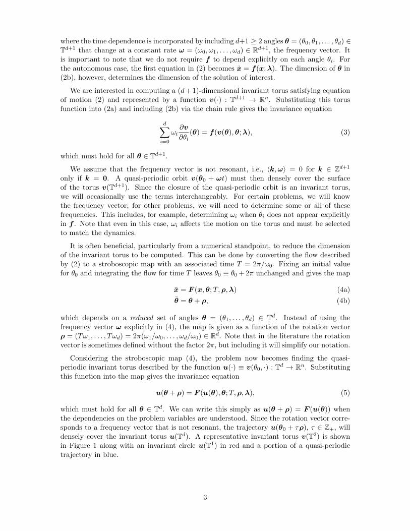
which must hold for all θ ∈ Td. We can write this simply as u(θ + ρ) = F (u(θ)) whenthe dependencies on the problem variables are understood. Since the rotation vector corre-sponds to a frequency vector that is not resonant, the trajectory u(θ0 + τρ), τ ∈ Z+, willdensely cover the invariant torus u(Td). A representative invariant torus v(T2) is shownin Figure 1 along with an invariant circle u(T1) in red and a portion of a quasi-periodictrajectory in blue.

3

Figure 1. Invariant torus of flow with invariant circle (red) of stroboscopic map.

An extensive theory known as Kolmogorov-Arnold-Moser theory deals with propertiesof quasi-periodic solutions to (2) and (4).3,4 While the current work is focused on thecomputation and application of the solutions, some aspects of the theory are relevant tothis work. We are particularly interested in the family structure of the tori. Assuming a(d+ 1)-dimensional quasi-periodic torus exists, for an autonomous Hamiltonian dynamicalsystem that depends on external parameters λ ∈ Rp, the torus (up to a maximum dimensionof n/2) will lie in a (p + d + 1)-parameter family. For example, without any free externalparameters, two-dimensional tori in the CR3BP lie in two-parameter families. For theER3BP, one of the torus’s frequencies is fixed by the period of the primary bodies. If theeccentricity of the primary bodies is constrained, two-dimensional tori lie in one-parameterfamilies.

Similar to equilibrium points and periodic orbits, quasi-periodic orbits can have stableand unstable motion in their vicinity. For example, a two-dimensional hyperbolic torus inthe CR3BP will have three-dimensional stable and unstable manifolds. Linearizing the map(4) about a quasi-periodic solution u gives

δu = F x(u(θ))δu (6a)

θ = θ + ρ (6b)

Since matrix F x (where the subscript x represents differentiation) varies with the locationθ on the torus u, it does not directly provide stability information. However, assuming a co-ordinate change δu(·) 7→ δw(·) exists such that this linearized equation can be transformedinto the form

δw = Bδw (7a)

θ = θ + ρ (7b)

where B ∈ Rn×n is a constant matrix, the torus is termed reducible, a property that wewill utilize when analyzing stability. The so-called Floquet matrix B fills a role similar tothe monodromy matrix of a periodic orbit. While we will not directly compute this matrix,we will determine its eigenvalues, which provide linear stability information.

4

Related work

A variety of methods are available for computing quasi-periodic tori in dynamical sys-tems. Only some of these approaches, however, have been applied to problems in astro-dynamics. Motivated by trajectory design applications, analytical work from the 1970sincludes Farquhar and Kamel’s third-order expansion of orbits in the vicinity of the Earth–Moon L2 libration point using a Poincare-Lindstedt method.5 During the same time period,Richardson and Cary developed a third-order approximation of quasi-periodic motion nearthe Sun–Earth L1 and L2 libration points via the method of multiple time scales.6 Morerecent semi-analytical work leverages computer algebra tools. Gomez et al. use a Poincare-Lindstedt method to generate high-order quasi-halo orbit expansions.7 Jorba and Masde-mont investigate the dynamics around the libration points using center manifold reduction.8

These local methods offer a thorough view of the dynamics in the libration point vicinity,but they are limited by their regions of convergence. Specialized algebraic manipulators areoften required as well, which can be an implementation obstacle. Still, the solutions havebeen successfully exploited for generating heteroclinic connections.9

In the 1980s Howell and Pernicka presented a numerical shooting approach for correct-ing approximate quasi-periodic orbits, though lacking control of orbit parameters.10 Gomezand Mondelo later developed a scheme for computing two-dimensional quasi-periodic toriby using an invariant circle parameterized by Fourier coefficients of a stroboscopic map.11

Kolemen et al. use a similar approach except with multiple Poincare maps and directly pa-rameterizing the invariant circle using states.12 The current approach uses similar conceptsto these methods but with a more general formulation. We use a stroboscopic map, whichrequires less knowledge of the solution structure than a sequence of Poincare maps, andconsider tori of arbitrary dimension. We use a grid of states on the invariant torus allowingus to avoid a convolution that is necessary when using a Fourier coefficient parameteriza-tion. In addition, we incorporate a different set of solution and continuation constraintsthat are broadly applicable. This allows the method to be used unchanged between familiesof solutions. An alternative approach presented by Schilder et al. computes a torus of aflow directly,13 and some of the constraints used have been adapted from this approach.The flow approach has been applied to the CR3BP;14 however, this requires dealing with atorus of dimension one larger than the torus of an associated map.

For computing the Floquet stability of tori, Jorba introduces a numerical approach basedon the eigenvalues of a large, dense matrix.15 This approach is adapted in the current workto deal directly with states rather than Fourier coefficients, and the matrix is a byproductof the torus computation scheme. Jorba and Olmedo also have an efficient method thatcombines the torus and stability computations, but it is specific to nonautonomous systemswith known forcing frequencies.16

While a majority of research has focused on the CR3BP, special solutions in the ER3BPhave also been considered. Early analytic expansions included the eccentricity of the primarybodies,5,6 and recently periodic orbits have been numerically investigated.17 Unlike theCR3BP, these orbits are isolated since most periodic orbits that persist become quasi-periodic orbits with the influence of eccentricity. Some examples of these quasi-periodicorbits are included in this paper.

5

COMPUTING QUASI-PERIODIC TORI

In this section we present a method for computing families of quasi-periodic invarianttori. The principal idea will be to find a d-dimensional torus that is invariant under thestroboscopic map F (4). The torus will be represented using a function u discretized overthe domain of torus angles and interpolated using a truncated Fourier series; however,we will be able to deal directly with a grid of states on the torus instead of the Fouriercoefficients since the discrete Fourier transform and its inverse are linear operations. Formany problems, including the CR3BP and ER3BP, we will need to include constraints suchthat there is a unique torus function u as a solution. We present a set of general-purposeconstraints that are applicable to a broad range of problems. These constraints include aphase condition on any free angles of the torus, which allows each torus to have a uniquerepresentation, and a constraint for fixing the values of any integrals of motions. Oncethe family is reduced to a single parameter, pseudo-arclength continuation is used to selectindividual family members. By applying a Newton method, we can iterate to find thetorus. This is incorporated into a predictor–corrector method to generate a family, whichis initialized from a periodic orbit.

Invariance condition

Finding a (d + 1)-dimensional quasi-periodic solution to the differential equation (2) isequivalent to finding a d-dimensional quasi-periodic solution to the map (4). This solutionfunction u must satisfy the invariance condition (5) where the stroboscopic time T andthe rotation vector ρ (or, equivalently, the frequency vector ω) and the parameters λ arepotentially unknown. The search for this solution can be posed as finding a fixed point ofan (infinite-dimensional) map acting on the space of functions U =

{u : Td → Rn

}, which

we assume to have sufficient smoothness. This map G : U → U is defined to be

G(u) = R(−ρ) ◦ F (u(·), · ;T,ρ,λ), (8)

where R(−ρ) : U → U is an invertible operator defined such that u(θ− ρ) = (R−ρ ◦u)(θ)for all θ ∈ Td. The fixed point invariance condition

G(u)− u = 0U (9)

comes from applying R(−ρ) to (5)—this removes the rotation about the torus under themap F . Note that G depends on the full set of “parameters” T , ρ, and λ.

A solution to (9) will be found using a Newton method. To do this we expand theequation in a Taylor series to first order neglecting higher-order terms. We use a superscriptzero to denote nominal values, subscripts to denote differentiation with respect to a variable,and δ to represent linear variations:

R(−ρ0) ◦{F 0x · δu+ F 0

T · δT +(F 0ρ − F 0

θ

)· δρ+ F 0

λ · δλ}− δu = −G0 (10)

Note that the term −F 0θ comes from differentiating the rotation operator R(−ρ) with

respect to ρ and composing the result with F 0. Solving this linear equation for the variationsgives a first-order correction to the variables to satisfy the invariance condition. Oncethe torus function u is suitably discretized, this equation can be represented by a matrixequation to solve for the torus update as part of a Newton method. We will later observe thatsystem (10) often does not have a unique solution and additional constraints are necessary.

6

Discretization

In the previous section, the invariance condition was posed as the fixed point of a mapG (8) on the space of smooth functions U =

{u : Td → Rn

}. A natural representation of

this space is via Fourier series, which we assume to converge appropriately for the functionsof interest in this paper. We can express torus function u as

u(θ) =∑k∈Zd

ckei〈k,θ〉 (11)

where the coefficients ck ∈ Cn have a vector index k = (k1, . . . , kd). In order to compute unumerically, we truncate the Fourier series such that each vector component ki can take onNi integer values centered about zero. For simplicity, we assume all the Ni are odd (thoughthe extension to Ni that are even is not difficult). We can define an index set

K ≡{k ∈ Zd| − Ni−1

2 ≤ ki ≤ Ni−12 for all i

}, (12)

which allows us to express the truncated Fourier series as

u(θ) =∑k∈K

ckei〈k,θ〉 (13)

where there is an array of N1 × · · · ×Nd coefficients ck that represent the discretized torusfunction u. We can also define a grid over the torus Td containing N1 × · · · ×Nd angles

θj = 2π(j1/N1, . . . , jd/Nd) (14)

where vector index j belongs to the set

J ≡{j ∈ Zd|0 ≤ ji < Ni for all i

}. (15)

There is an invertible correspondence between the array of coefficients {ck}k∈K and thearray of states {uj = u(θj)}j∈J on the torus via the discrete Fourier transform (DFT).Furthermore, the transform is a linear operation. If these arrays are rearranged as vectors{c} and {u}, we can write the DFT operation as

{c} = [D] {u} (16)

where [D(N1, . . . , Nd)] is a matrix that depends only on the number of Fourier coefficients,or equivalently, the number of grid points. Note that we use complex Fourier coefficients dueto the greater ease of implementation but that real Fourier coefficients could also be used.Using the correspondence between the Fourier coefficients and the states, the approximationin (13) provides a trigonometric interpolation between the grid of states on the torus.

Discretized rotation operator. Rotation R(−ρ) : U → U , defined such that u(θ − ρ) =(R−ρ◦u)(θ), is included in (8) to cancel out the rotation about the torus under map F . Thisoperation can easily be performed using the Fourier coefficients. Substituting the definitioninto (13), each coefficient is simply transformed by Q(−ρ) : ck 7→ cke

i〈k,−ρ〉. Representedas a matrix, [Q(−ρ;N1, . . . , Nd)] is diagonal operating on coefficient vector {c} and only

7

depends on the rotation vector ρ and the number of Fourier coefficients. Combining thismatrix with the DFT transform matrices as follows,

[R(−ρ)] = [D−1][Q(−ρ)][D], (17)

gives a matrix that rotates the grid of states on the torus by rotation vector −ρ via trigono-metric interpolation; i.e., {u2} = [R(−ρ)] {u1} implies that u1(θ − ρ) = u2(θ) for all θ.Note that while the DFT matrices and [Q] are complex, the product [R(−ρ)] must be real.

Newton method. Discretizing the torus function u via a truncated Fourier series allowsthe first-order Taylor series expansion (10) of the invariance equation (9) to be put into amatrix form that will be incorporated as part of a Newton method. The discretized variationof the torus function {δuj = δu(θj)}j∈J can be rearranged from an N1 × · · · ×Nd array of

vectors in Rn to a single vector {δu} ∈ RnN1···Nd giving the linear system

([R(−ρ0)

]·[F 0x F 0

T F 0ρ − F 0

θ F 0λ

]−[I 0 0 0

])δuδTδρδλ

= −{G0}

(18)

where the first submatrix

[F 0x

]=

F0x(θ0)

. . .

F 0x(θN−1)

(19)

is block diagonal with the linearization of the stroboscopic map F 0x(θj) ≡ F x(u0(θj),θj ;

T 0,ρ0,λ0) evaluated at each point over the torus grid from j = (0, . . . , 0) to (N1−1, . . . , Nd−1),. In a similar manner we can construct submatrices

[F 0∗]

=

F 0∗(θ0)

...F 0∗(θN−1)

(20)

(where ∗ denotes T , ρ, θ, or λ) by stacking up the derivative with respect to the variable ofinterest, F 0

∗(θj) ≡ F ∗(u0(θj),θj ;T0,ρ0,λ0), evaluated at each grid point over the torus.

The full matrix from (18) has dimension (nN1N2 · · ·Nd) × (nN1 · · ·Nd + 1 + d + p). Thissystem does not have a unique solution, so constraints will be added to make the solutionunique. This will lead to adding rows to this matrix corresponding to the constraints. It isalso worth noting that the submatrix product [R(−ρ)][F x] will be used after convergenceto a quasi-periodic torus for computing stability information.

Integrating variations

In order to transition from the vector field f to the stroboscopic map F , it is necessaryto determine how the problem variables influence the map. These sensitivities appear in thesubmatrices (19)–(20) of linear system (18). We denote the solution flow by φ(x0,θ0; t,ρ,λ),

8

or simply φ(t), with initial conditions x0 ∈ Rn, θ0 ∈ Td+1 at time t = 0. The state transitionmatrix Φ(t) ≡ φx0

(t) satisfies the differential equation

d

dtΦ = AΦ (21)

where A ≡ fx and with initial value Φ(0) = I and final value denoted F x ≡ Φ(T ). Thedependence on the parameters λ is available from the equation

d

dtφλ = Aφλ + fλ (22)

with initial value φλ(0) = 0 and final value denoted F λ ≡ φλ(T ). Similarly, we canintegrate the dependence on the frequency vector ω using

d

dtφω = Aφω + fω = Aφω + fθt (23)

with initial value φω(0) = 0 and final value denoted Fω ≡ φω(T ). Noting the relationshipbetween the frequency vector ω, the stroboscopic time T , and the rotation vector ρ, we canderive the relations

F T = f(φ(T ))−d∑i=0

ωiTF ωi , (24)

F ρi =1

TF ωi (25)

for i = 1, . . . , d. Finally, the term F θ, θ ∈ Td, that appears in (18) can be obtained bydifferentiating the Fourier representation of F (u).

Constraints

We incorporate constraints to provide a unique numerical representation of a torus.These constraints serve two purposes. One is to select a particular quasi-periodic torusfrom within a one- or more-parameter family of tori. The second purpose is to provide aunique parameterization of a particular torus. For example, the phases of a torus’s anglesin an autonomous system are free and need to be constrained. Selecting the appropriate setof constraints requires some basic knowledge of the dynamical system’s solution structure.With an appropriate set, the Newton method should converge appropriately.

Fixing one of the problem variables such as a component of the state u(θj), the stro-boscopic time T , an element of the rotation vector ρ, or a parameter from λ are the mostbasic constraints and are straightforward to implement. All we need to do is fix its variationas zero, e.g., δT = 0. One simply appends a row of all zeros to the matrix in (18) exceptfor a one corresponding to the variable to fix, and a zero is appended to the vector on theright-hand side.

However, more complicated and potentially more robust constraints require greater care.We often use constraints that depend on the integral of a function g : Rn → R over thetorus’s surface. This gives the function’s average value, which over the space U of truncated

9

Fourier series can be shown to simply be the average value of the function evaluated overthe torus grid,

1

(2π)d

ˆTd

g(u(θ))dθ =1

N1 · · ·Nd

∑j∈J

g(u(θj)). (26)

We will use an integral of this form for constraining an integral of motion. As an extensionof this, we often use an inner product 〈· , ·〉U : U × U → R as defined by:

〈u1,u2〉U =1

(2π)d

ˆTd

〈u1(θ),u2(θ)〉 dθ =1

N1 · · ·Nd

∑j∈J〈u1(θj),u2(θj)〉 . (27)

We will use this inner product for constraints on angle phases and for pseudo-arclengthcontinuation.

Phase constraint. For a system that is not completely forced (i.e., where certain angles θido not appear explicitly in the equations of motion), there is an indeterminacy in the torusfunction representation u of the invariant torus. For example, consider a two-dimensionalquasi-periodic torus of an autonomous system. Using a stroboscopic map, there is aninvariant circle. However, this circle can be shifted around the torus and still be invariant.Furthermore, the angle parameterizing the circle can be defined relative to any point on thecircle. Systems exhibiting these sort of indeterminacies need constraints to fix a particularsolution.

The simplest options involve a constraint on a single point of the torus. However, a morerobust condition depends on the integral over the torus.13 Assuming the torus functionu of a nearby family member is known, we seek to minimize

´Td ‖u− u‖2 dθ over the

possible freedoms in phase of u. From the necessary conditions, it can be shown that thecorresponding phase constraint for each angle θi is⟨

u,∂u

∂θi

⟩= 0, (28)

which uses the inner product defined earlier in (27). Expanding up to first-order gives theequation

1

N1 · · ·Nd

∑j∈J

⟨∂u

∂θi(θj), δu(θj)

⟩= −

⟨∂u

∂θi,u0

⟩, (29)

which can be appended to the linear system in (18). Computing ∂u/∂θi is readily availablefor i = 1, . . . , d from the Fourier representation of u. Computing ∂u/∂θ0 requires theinvariance equation (3) for quasi-periodic motion in a flow, which gives

∂u

∂θ0(θ) =

1

ω0

(f(u(θ), (θ0,θ);λ)−

d∑i=1

ωi∂u

∂θi(θ)

)(30)

where θ0 is the section used for the stroboscopic map, and θ = (θ1, . . . , θd) ∈ Td. Recallthat ω = (2π,ρ)/T .

10

Integral of motion constraint. Since an integral of motion is an invariant of the flow,fixing its value reduces the phase space to an invariant manifold of dimension one less.For example, fixing the Hamiltonian value would let us find the quasi-periodic solutionsthat exist at a certain “energy” level. This corresponds to fixing the Jacobi constant inthe CR3BP, which reduces the two-parameter families of quasi-periodic tori to a singleparameter.

Let us assume (2) admits an integral of motion H. While it suffices to fix the integral’svalue to H at a single state on the torus (since the torus can be viewed as the closure of asingle trajectory), it is more numerically robust to consider the value over the entire torusand incorporate a constraint of the form

H =1

(2π)d

ˆTd

H(u(θ))dθ. (31)

Expanding this as a Taylor series and using (26) gives

1

N1 · · ·Nd

∑j∈J

∂H

∂x(u0(θj))δu(θj) = H − 1

N1 · · ·Nd

∑j∈J

H(u0(θj)). (32)

This can be used to add a row to the matrix for correcting the torus. The constraint enforcesthat, up to first order, the updated torus will have the correct average integral value.

Pseudo-arclength continuation. Once the set of quasi-periodic orbits is reduced to asingle-parameter family, a continuation scheme can be applied. Some approaches explic-itly use problem parameters or ad hoc selection of a particular family’s characteristics.Pseudo-arclength continuation offers the benefit of not explicitly depending on any partic-ular parameter but rather stepping along the family tangent. This allows the family toproceed around turning points relative to a parameter. Pseudo-arclength continuation hasbeen used effectively for generating families of periodic orbits, including in the CR3BP.18

Let us assume that we know a previous member of the family (u, T , ρ, λ) along with an

approximate, normalized family tangent direction (u′, T ′, ρ′, λ′). Pseudo-arclength continu-

ation requires the change to the next family member (u, T,ρ,λ) projected along the familytangent to be of length ∆s, the step size:

∆s = ku⟨u′,u− u

⟩+ kT

⟨T ′, T − T

⟩+ kρ

⟨ρ′,ρ− ρ

⟩+ kλ

⟨λ′,λ− λ

⟩. (33)

In the above equation, constants ku, kT , kρ, kλ are incorporated to allow more control overthe stepping process. We can expand this up to first order as a Taylor series to get

ku⟨u′, δu

⟩+ kT

⟨T ′, δT

⟩+ kρ

⟨ρ′, δρ

⟩+ kλ

⟨λ′, δλ

⟩= ∆s−∆s0. (34)

The constraint can be implemented by adding a row to the matrix in (18). Note that thefamily tangent does not need to be exact since it just affects the step size and not the quasi-periodic orbit invariance conditions. It often suffices to simply normalize the differencebetween the previous two members of the family.

11

Generating family

With an appropriate set of constraints, a dynamical system’s quasi-periodic tori can bereduced to a single parameter family, each member having a unique torus function repre-sentation. Incorporating pseudo-arclength continuation allows us to select a single memberfrom the family at each step. Computing each member requires solving the nonlinear in-variance equation (9), which we approach using a predictor–corrector method. Assuminga previous member (u, T , ρ, λ) of the family is known along with an approximation of the

family tangent (u′, T ′, ρ′, λ′), we use a simple linear prediction of the next member. The

prediction is iteratively corrected using the Newton method. This requires solving linearsystem (18) with the constraints appended. For systems possessing special structure, in-cluding the CR3BP and ER3BP, the appropriate set of constraints will lead to a matrixwith more rows than columns. A solution, however, exists. To solve a non-square system,we use a QR factorization. For square systems, an LU factorization is sufficient. Once thequasi-periodic solution is converged, the next member of the family can be predicted, andthe process repeats.

The most basic approach to initializing a quasi-periodic torus is from a periodic orbit.For the ER3BP, an initial approximation is available simply using a CR3BP periodic orbitsince this is generically no longer a solution once periodic forcing due to eccentric effects isincluded. Initializing a quasi-periodic torus in an autonomous system, such as the CR3BPitself, is possible from a periodic orbit with a center component. For a complex eigenvalueeiρ of the monodromy matrix Φ(T ) on the unit circle, let y ∈ Cn be the correspondingeigenvector. Then we can obtain a linear approximation of the one-dimensional invarianttorus relative to the fixed point on the periodic orbit:

u(θ1) = Re[eiθ1y

]= cos θ1Re [y]− sin θ1Im [y] , (35)

which can be scaled by a small value for initializing the first torus. The correspondingrotation number is ρ. This approach can be generalized to yield initial approximations ofhigher-dimensional tori from periodic orbits whose monodromy matrix has more than onepair of complex conjugate eigenvalues.

COMPUTING STABILITY AND ASSOCIATED MANIFOLDS

We now investigate the linearized dynamics in the vicinity of a computed quasi-periodicinvariant torus. We are particularly interested in hyperbolic tori and determining theirassociated stable and unstable directions. The method assumes the tori are reducible,which is a common property.16 Using the discretized invariant torus of the stroboscopicmap, stability information can be determined from an appropriate matrix. For hyperbolictori, we will show how to map the stable and unstable directions relative to the invarianttorus of the map to the full invariant torus of the flow. By perturbing the torus in thesedirections and integrating forward or backward in time, we can numerically generate theglobal manifolds.

Linear stability of torus

In the previous section, computing a quasi-periodic torus invariant under stroboscopicmap F (4) was reduced to finding the fixed point of a map G (9) on the space U of torus

12

functions. We can proceed to find the stability of the torus by studying the eigenvalues andeigenfunctions of the map’s linearization,

Gx(u(·)) ≡ R(−ρ) ◦ F x(u(·)). (36)

This operator incorporates the linearization of the stroboscopic map, F x(u(·)), but alsoremoves the rotation about the invariant torus by including the composition with R(−ρ).This way we can compare the behavior of a perturbation under the map relative to theoriginal torus function u(·) as opposed to u(· + ρ); i.e., perturbation δu(θ) and mappedperturbation δu(θ) have the same base point u(θ).

Jorba shows that the eigenvalues of (36) correspond to the eigenvalues of the Floquetmatrix B defined in (7) up to a rotation of the form ei〈k,ρ〉, k ∈ Zd.15 Therefore, the fullspectrum lies densely on circles in the complex plane. For a real, non-unity eigenvalue of(36), if the entire torus u(·) is perturbed in the direction of the corresponding eigenfunctionδu(·), an iteration of the map simply expands or contracts in this direction. This is a linearapproximation of stable and unstable manifold directions.

When the torus function space is discretized via truncated Fourier series, operator (36)can be represented by the matrix [Gx] = [R(−ρ)] [F x]. This matrix, appearing in thelinear system (18), is a byproduct of the torus computation scheme. It is evaluated usingthe converged, discretized torus u such as from the last Newton iteration. It is importantto note that this matrix acts directly on variations of the torus states. Jorba uses a similaroperator except in terms of Fourier coefficients. If we represent the N1 × · · · ×Nd array ofstate variations as vectors {δu} and {δu}, they are related by

{δu} = [Gx] {δu} . (37)

This matrix is of dimension (nN1 · · ·Nd) × (nN1 · · ·Nd) and has nN1 · · ·Nd eigenvaluessince it is finite dimensional. This matrix is also dense and potentially quite large, butschemes exists for determining its eigenstructure. The eigenvalues of [Gx] correspond to theeigenvalues of the Floquet matrix B up to a rotation about the origin in the complex plane.The magnitude of the eigenvalues, however, is maintained providing stability information.If sets of eigenvalues off the unit circle exist, it corresponds to stable and unstable motionin the vicinity. The eigenvectors corresponding to real eigenvalues in the sets give the stableand unstable manifold tangent directions at each of the grid points on the torus.

Transition to full torus

Thus far we have only considered the manifold tangent directions δu(·) relative to torusfunction u(·) ≡ v(θ0, ·) : Td → Rn of the stroboscopic map. However, we would like togenerate the tangent directions δv(·) relative to the full torus of the flow, v(·) : Td+1 → Rn.This can easily be performed using the state transition matrix Φ. For any θ′ ∈ Td+1, thereexists some t ∈ [0, T ) and θ ∈ Td such that θ′ = (θ0,θ)+ωt. Then we have the relationship

δv(θ′) = Φ(θ; t)δu(θ), (38)

which is simply the tangent direction δu(θ) relative to point u(θ) mapped forward to apoint v(θ′) on the full torus of the flow. Since the state transition matrix also scales the

13

tangent direction, for each θ′0 we can normalize δv(θ′0, ·) by factor

ˆTd

∥∥δv(θ′0,θ)∥∥ dθ =

1

N1 · · ·Nd

∑j∈J

∥∥v(θ′0,θj)∥∥ . (39)

Finally, to initialize the stable or unstable manifold, we can choose a small term ε > 0, andlinearly approximate points on the manifold using v(θ′) + ε δv(θ′). We can then simplypropagate forward or backward in time to globalize the manifold. The manifold will be ofdimension d+ 2 for the (d+ 1)-dimensional invariant torus in the phase space.

RESULTS

In this section we illustrate the numerical method for computing quasi-periodic orbitsand their stability by considering examples in the restricted three-body problem. We con-sider both the CR3BP and the ER3BP with a mass ratio corresponding to the Earth–Moonsystem. For the ER3BP, however, we continue solutions beyond the system’s true eccen-tricity. For both problems, families of tori are generated along with associated stable andunstable manifolds.

Circular restricted three-body problem

In the CR3BP, the gravitational interaction of three bodies, one with infinitesimal mass,is modeled. We assume that the two massive, primary bodies travel in circular orbits. Thethird body is located at q = (x, y, z) in a barycentric rotating frame, which is defined suchthat the primary bodies are fixed along the x-axis. Its state x = (q,v) ∈ R6 is governed bythe nondimensional equation of motion(

qv

)= x = f(x) =

(v

Uq + 2v × z

), (40)

which depends on a force potential-like function

U(q) =1− µr1

+µ

r2+

1

2

(x2 + y2

). (41)

The parameter µ ∈ [0, 0.5] relates the primaries’ masses, r1 and r2 are the distances of thethird body to each primary (the larger and smaller primaries are located at x = −µ andx = 1−µ, respectively), and z is a unit vector along the z-axis, the direction of the systemangular momentum. For the Earth–Moon system, we use mass parameter µ = 0.01215,which is fixed for all solutions and, thus, not included in λ as a free parameter. The first-order ordinary differential equation (40) admits an integral of motion, C(x) = 2U(q)−‖v‖2 ,which is often denoted the Jacobi constant. The CR3BP’s five well-known equilibriumpoints are the L1–L5 libration points. All of the libration points contain center componentsassociated with emanating families of periodic orbits.18 Similarly, many of these periodicorbits also possess center components, which correspond to quasi-periodic motion in theirvicinity.

For generating the quasi-periodic families, we append equation (2b), (θ0, θ1) = (ω0, ω1)with both torus frequencies unknown, to the equation of motion (40). We use phase con-straints on angles θ0 and θ1. We also use the integral of motion constraint to fix the Jacobi

14

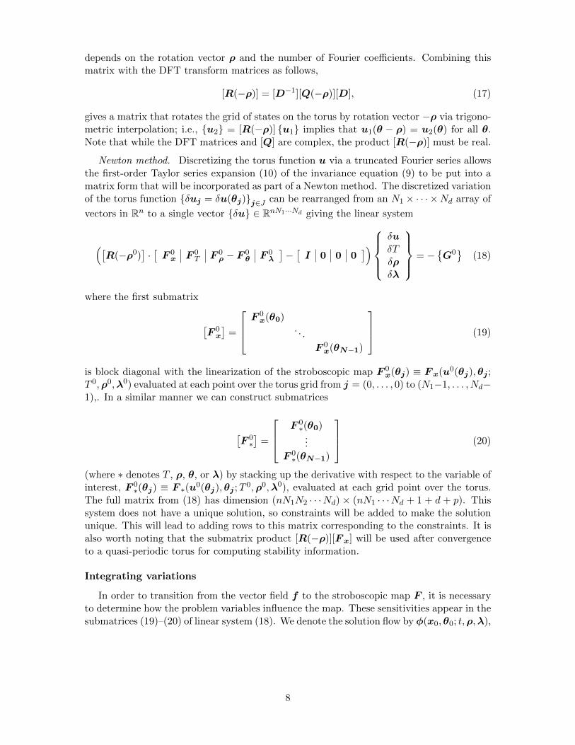
Figure 2. Members of quasi-halo torus family emanating from L2 halo orbit.

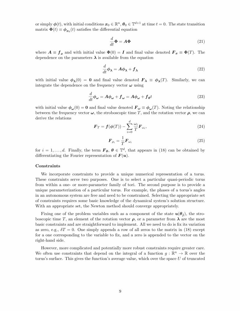
Figure 3. Tangent directions for stable and unstable manifolds of quasi-halo torus.

constant value for the family. This reduces the two-parameter family of two-dimensionalquasi-periodic orbits to a single parameter, which can be stepped along with pseudo-arclength continuation. Starting from an L2 halo periodic orbit in the Earth–Moon system,we generate representative members of the quasi-halo family, all members having Jacobiconstant C = 3.132, shown in Figure 2. A segment of the quasi-periodic trajectory on thetorus surface is also plotted.

Like the associated halo orbit, these quasi-periodic orbits are hyperbolic. In Figure 3we show the stable and unstable directions relative to one member of the quasi-halo family.Perturbing the torus along the tangent directions and propagating backward or forwardin time allows us to generate the three-dimensional stable or unstable manifold. If wepropagate the perturbed torus for discrete amounts of time, its image is also a torus. Thecontinuous sequence of these tori sweep out the manifold. Note that the tangent directionscan be flipped, i.e., multiplied by −1, to generate the other “half” of the stable or unstablemanifold. Part of a quasi-halo’s unstable manifold departing away from the smaller primary,the Moon, is shown in Figure 4. Manifold trajectories associated with one invariant circleon the torus are included. In Figure 5 we present the torus’s stable manifold arriving fromthe direction of the Moon. Note that the manifold becomes twisted in the Moon’s vicinity.

15

Figure 4. Snapshots of L2 quasi-halo unstable manifold departing away from Moon.

Figure 5. Snapshots of L2 quasi-halo stable manifold arriving from Moon’s vicinity.

16

Figure 6. Snapshots of L1 Lissajous unstable manifold departing towards Earth.

The method can be directly applied to other families with only a change in the initialorbit. Initializing the family from a planar L1 Lyapunov orbit, we show a two-dimensionalmember from the Lissajous family in Figure 6 along with its three-dimensional unstablemanifold departing in the direction of the Earth.

Elliptic restricted three-body problem

The two primary bodies in the ER3BP move on elliptic orbits with eccentricity e abouttheir barycenter. We consider the motion of a third body with infinitesimal mass. As withthe CR3BP, the primaries are fixed along the x-axis, and lengths are normalized by thedistance between them. However, this distance is now time-varying, which allows the thefive libration points to remain equilibrium solutions in the nondimensional rotating referenceframe. The ER3BP equation of motion is given by(

qv

)= x = f(x, θ1; e) =

(v

(1 + e cos θ1)−1(Uq − ze cos θ1 z) + 2v × z

)(42a)

where U is defined by (41), and we can append an equation for the dynamics on a quasi-periodic solution: (

θ0θ1

)= θ = ω =

(ω0

1

). (42b)

Note that the true anomaly θ1 of the primaries, rather than time, is used as the independentvariable in these equations. However, it is simple to switch between these two. We can alsonote that when parameter e = 0 in (42a), we recover the CR3BP equation of motion (40).

Since two-dimensional quasi-periodic tori in the ER3BP fill a role similar to periodicorbits in the CR3BP, we can initialize the ER3BP quasi-periodic orbits from the CR3BPperiodic orbits. For obtaining families, we fix the stroboscopic time T to match the periodicorbit’s period and the frequency ω1 = 1 to match the primaries’ frequency. The eccentricitye is allowed to vary. We include a phase constraint for angle θ0. A constraint for angle θ1

17

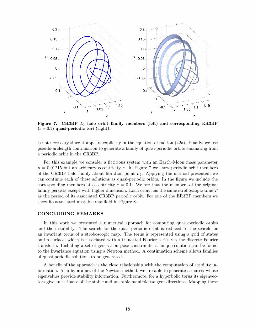
Figure 7. CR3BP L2 halo orbit family members (left) and corresponding ER3BP(e = 0.1) quasi-periodic tori (right).

is not necessary since it appears explicitly in the equation of motion (42a). Finally, we usepseudo-arclength continuation to generate a family of quasi-periodic orbits emanating froma periodic orbit in the CR3BP.

For this example we consider a fictitious system with an Earth–Moon mass parameterµ = 0.01215 but an arbitrary eccentricity e. In Figure 7 we show periodic orbit membersof the CR3BP halo family about libration point L2. Applying the method presented, wecan continue each of these solutions as quasi-periodic orbits. In the figure we include thecorresponding members at eccentricity e = 0.1. We see that the members of the originalfamily persists except with higher dimension. Each orbit has the same stroboscopic time Tas the period of its associated CR3BP periodic orbit. For one of the ER3BP members weshow its associated unstable manifold in Figure 8.

CONCLUDING REMARKS

In this work we presented a numerical approach for computing quasi-periodic orbitsand their stability. The search for the quasi-periodic orbit is reduced to the search foran invariant torus of a stroboscopic map. The torus is represented using a grid of stateson its surface, which is associated with a truncated Fourier series via the discrete Fouriertransform. Including a set of general-purpose constraints, a unique solution can be foundto the invariance equation using a Newton method. A continuation scheme allows familiesof quasi-periodic solutions to be generated.

A benefit of the approach is the close relationship with the computation of stability in-formation. As a byproduct of the Newton method, we are able to generate a matrix whoseeigenvalues provide stability information. Furthermore, for a hyperbolic torus its eigenvec-tors give an estimate of the stable and unstable manifold tangent directions. Mapping these

18

Figure 8. Snapshots of ER3BP quasi-halo unstable manifold departing away fromMoon.

around the full torus and propagating a small displacement in these directions provides anapproximation of the global stable and unstable manifolds.

While the scheme is designed for a general class of systems, it was illustrated usingexamples from the circular and elliptic restricted three-body problems. These examplesdemonstrate the ability to compute manifolds associated with quasi-halo and Lissajous or-bits. One of the primary motivations behind this work is the preliminary development oftools to help incorporate quasi-periodic orbits in astrodynamics mission design. Relativeto equilibrium points and periodic orbits, the prevalence of quasi-periodic orbits and theirassociated manifolds in the restricted three-body problem can greatly expand the designspace, ultimately leading to more efficient trajectories. Future work includes studying con-necting orbits between the tori and solutions in other astrodynamical systems. The methoditself can be made more robust by incorporating multiple shooting. An error analysis is alsowarranted.

ACKNOWLEDGMENTS

This work was conducted at the University of Colorado Boulder with support from theDepartment of Aerospace Engineering Sciences and the National Science Foundation (NSF)Graduate Research Fellowship Program.

REFERENCES

[1] G. Gomez, A. Jorba, J. J. Masdemont, and C. Simo, “Study of the Transfer from the Earth to a HaloOrbit Around the Equilibrium Point L1,” Celestial Mechanics and Dynamical Astronomy, Vol. 56, No.4, 1993, pp. 541–562.

[2] K. C. Howell, B. T. Barden, and M. W. Lo, “Application of Dynamical Systems Theory to TrajectoryDesign for a Libration Point Mission,” Journal of the Astronautical Sciences, Vol. 45, No. 2, 1997, pp.161–178.

19

[3] H. W. Broer, G. B. Huitema, and M. B. Sevryuk, Quasi-Periodic Motions in Families of DynamicalSystems, Berlin: Springer-Verlag, 1996.

[4] R. de la Llave, “A Tutorial on KAM Theory,” in Smooth Ergodic Theory and Its Applications, Proceed-ings of Symposia in Pure Mathematics, Providence: AMS, 2001.

[5] R. W. Farquhar and A. A. Kamel, “Quasi-Periodic Orbits About the Translunar Libration Point,” Ce-lestial Mechanics and Dynamical Astronomy, Vol. 7, No. 4, 1973, pp. 458–473.

[6] D. L. Richardson and N. D. Cary, “A Uniformly Valid Solution for Motion About the Interior LibrationPoint of the Perturbed Elliptic-Restricted Problem,” AAS/AIAA Astrodynamics Specialist Conference,Nassau, Bahamas, July 28–30, 1975.

[7] G. Gomez, J. J. Masdemont, and C. Simo, “Quasihalo Orbits Associated with Libration Points,”Journalof the Astronautical Sciences, Vol. 46, No. 2, 1998, pp. 135–176.

[8] A. Jorba and J. J. Masdemont, “Dynamics in the Center Manifold of the Restricted Three-Body Prob-lem,” Physica D, Vol. 132, No. 1–2, 1999, pp. 189–213.

[9] G. Gomez, W. S. Koon, M. W. Lo, J. E. Marsden, J. Masdemont, and S. D. Ross, “Connecting Orbitsand Invariant Manifolds in the Spatial Restricted Three-Body Problem,” Nonlinearity, Vol. 17, No. 5,2004, pp. 1571–1606.

[10] K. C. Howell and H. J. Pernicka, “Numerical Determination of Lissajous Trajectories in the RestrictedThree-Body Problem,” Celestial Mechanics and Dynamical Astronomy, Vol. 41, No. 1–4, 1988, pp.107–124.

[11] G. Gomez and J. M. Mondelo, “The Dynamics Around the Collinear Equilibrium Points of the RTBP,”Physica D, Vol. 157, No. 4, 2001, pp. 283–321.

[12] E. Kolemen, N. J. Kasdin, and P. Gurfil, “Multiple Poincare Sections Method for Finding the Quasiperi-odic Orbits of the Restricted Three-Body Problem,” Celestial Mechanics and Dynamical Astronomy,Vol. 112, No. 1, 2012, pp. 47–74.

[13] F. Schilder, H. M. Osinga, and W. Vogt, “Continuation of Quasi-Periodic Invariant Tori,”SIAM Journalon Applied Dynamical Systems, Vol. 4, No. 3, 2005, pp. 459–488.

[14] Z. P. Olikara and K. C. Howell, “Computation of Quasi-Periodic Invariant Tori in the Restricted Three-Body Problem,” AAS/AIAA Space Flight Mechanics Meeting, San Diego, CA, February 14–18, 2010.

[15] A. Jorba, “Numerical Computation of the Normal Behavior of Invariant Curves of n-Dimensional Maps,”Nonlinearity, Vol. 14, No. 5, 2001, pp. 943–976.

[16] A. Jorba and E. Olmedo, “On the Computation of Reducible Invariant Tori in a Parallel Computer,”SIAM Journal of Applied Dynamical Systems, Vol. 8, No. 4, 2009, pp. 1382–1404.

[17] S. Campagnola, M. W. Lo, and and P. Newton, “Subregions of Motion and Elliptic Halo Orbits in theElliptic Restricted Three-Body Problem,” AIAA/AAS Space Flight Mechanics Meeting, Galveston, TX,January 27–31, 2008.

[18] E. J. Doedel, V. A. Romanov, R. C. Paffenroth, H. B. Keller, D. J. Dichmann, J. Galan-Vioque, andA. Vanderbauwhede, “Elemental Periodic Orbits Associated with the Libration Points in the CircularRestricted 3-Body Problem,” International Journal of Bifurcation and Chaos, Vol. 17, No. 8, 2007, pp.2625–2677.

20