numerical methods for maxwell's equationsmath.oregonstate.edu/~gibsonn/553talk.pdf ·...

Numerical Methods for Maxwell’s Equations

Prof. Nathan L. Gibson

Department of Mathematics

MTH 453/553May 27, 2015

Prof. Gibson (OSU) CEM MTH 453/553 1 / 54

Acknowledgements

Collaborators

H. T. Banks (NCSU)

V. A. Bokil (OSU)

W. P. Winfree (NASA)

Students

Karen Barrese and Neel Chugh (REU 2008)

Anne Marie Milne and Danielle Wedde (REU 2009)

Erin Bela and Erik Hortsch (REU 2010)

Megan Armentrout (MS 2011)

Brian McKenzie (MS 2011)

Duncan McGregor (MS 2014, PhD 2016)


Outline

1 PreliminariesPDEs

2 Maxwell’s EquationsSimplifications

3 Numerical MethodsThe Yee Scheme2M Order Approximations in Space(2, 2M) Order Methods for Debye Polarization Modelsvon Neumann Stability Analysis


Preliminaries

Outline

1 PreliminariesPDEs




Preliminaries PDEs

A General First Order Linear PDE System

∂u

∂t−Au = f

where u is called a state variable, A is a linear operator depending on a setof parameters q, and f is a source term.Examples

A = c ∂∂x yields a one-way wave equation.

u = [H,E ]T and

A =

[0 1

µ∂∂x

1ε∂∂x 0

]yields 1D Maxwell’s equations in a dielectric, equivalent to the waveequation with speed c =

√(1/εµ).

u = [H,E]T

A =

[0 1

µ∇×1ε∇×

σε

]yields 3D Maxwell curl equations in a non-dispersive dielectric.Prof. Gibson (OSU) CEM MTH 453/553 5 / 54

Preliminaries PDEs

Electromagnetic Applications

Computers

Cell Phones

Aging Aircraft

Biomedical

Astronomy

Resources Exploration

GPS

Gas Milage


Maxwell’s Equations

Outline

1 PreliminariesPDEs






Maxwell’s Equations were

formulated circa 1870.

They represent a fundamental

unification of electric and

magnetic fields predicting

electromagnetic wave

phenomenon.




∂D

∂t+ J = ∇×H (Ampere)

∂B

∂t= −∇× E (Faraday)

∇ ·D = ρ (Poisson)

∇ · B = 0 (Gauss)

E = Electric field vector

H = Magnetic field vector

ρ = Electric charge density

D = Electric flux density

B = Magnetic flux density

J = Current density

With appropriate initial conditions and boundary conditions.



Constitutive Laws

Maxwell’s equations are completed by constitutive laws that describe theresponse of the medium to the electromagnetic field.

D = εE + P

B = µH + M

J = σE + Js

P = Polarization

M = Magnetization

Js = Source Current

ε = Electric permittivity

µ = Magnetic permeability

σ = Electric Conductivity


Maxwell’s Equations Simplifications

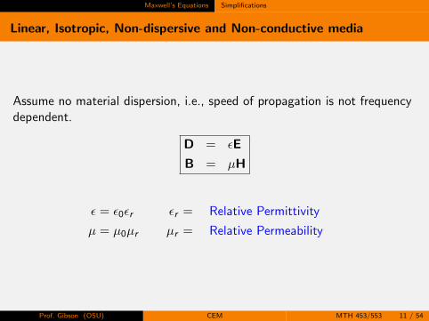
Linear, Isotropic, Non-dispersive and Non-conductive media

Assume no material dispersion, i.e., speed of propagation is not frequencydependent.

D = εE

B = µH

ε = ε0εr

µ = µ0µr

εr = Relative Permittivity

µr = Relative Permeability



Evolution in Time

The time evolution of the fields is thus completely specified by thecurl equations

ε∂E

∂t= ∇×H

µ∂H

∂t= −∇× E

The system above can be combined to a single second order equationfor E

ε∂2E

∂t2+∇× 1

µ∇× E = −∂J

∂t

This is often referred to as the curl-curl equation or the vector waveequation.



Maxwell’s Equations in One Space Dimension

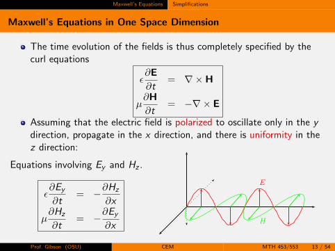
The time evolution of the fields is thus completely specified by thecurl equations

ε∂E

∂t= ∇×H

µ∂H

∂t= −∇× E

Assuming that the electric field is polarized to oscillate only in the ydirection, propagate in the x direction, and there is uniformity in thez direction:

Equations involving Ey and Hz .

ε∂Ey

∂t= −∂Hz

∂x

µ∂Hz

∂t= −∂Ey

∂x

x

y

x

Ey

H z

...................

.........

......

........

...

.................. ........ ......... ............ ...............

.....................................

.......................

..........................

.............................

..............................

..........................

.......................

................................................... ........... ......... ........ ........

..........

.........

...

.........

......

.....................................

.........

......

........

...

.................. ........ ......... ............ ...............

.....................................

.......................

..........................

.............................

..............................

..........................

.......................

................................................... ........... ......... ........ ........

..........

.........

...

.........

......

..................


Numerical Methods

Outline

1 PreliminariesPDEs




Numerical Methods The Yee Scheme

Finite Difference Methods

The Yee Scheme

In 1966 Kane Yee originated a set of finite-difference equations for thetime dependent Maxwell’s curl equations.

The finite difference time domain (FDTD) or Yee algorithm solves forboth the electric and magnetic fields in time and space using thecoupled Maxwell’s curl equations rather than solving for the electricfield alone (or the magnetic field alone) with a wave equation.



Yee Scheme in One Space Dimension

Staggered Grids: First order derivatives are much more accuratelyevaluated on staggered grids, such that if a variable is located on theinteger grid, its first derivative is best evaluated on the half-grid andvice-versa.

Staggered Grids of R with space step size ∆z = h

Primary Grid Gp = {z` = `h | ` ∈ Z},

Dual Grid Gd =

{z`+ 1

2=

(`+

1

2

)h | ` ∈ Z

}.

-

-�h

z� � � � � �v v v v v. . . z− 5

2

z−2 z− 32

z−1 z− 12

z0 z1z 12

z2z 32

z 52. . .




Staggered Grids: The electric field/flux is evaluated on the primarygrid in both space and time and the magnetic field/flux is evaluatedon the dual grid in space and time.

The Yee scheme is

H|n+ 12

`+ 12

− H|n−12

`+ 12

∆t= − 1

µ

E |n`+1 − E |n`∆z

E |n+1` − E |n`

∆t= −1

ε

H|n+ 12

`+ 12

− H|n+ 12

`− 12

∆z

-�h

tn+ 12

tn+1

� � � � � �

v v v v v. . . z− 5

2

z−2 z− 32

z−1 z− 12

z0 z1z 12

z2z 32

z 52. . .



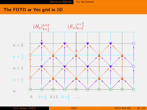
The FDTD or Yee grid in 1D

¡¡µ

¡¡µ

¡¡µ

¡¡µ

@@I

@@I

@@I

@@I

N N N Nf

f

¡¡µ

¡¡µ

¡¡µ

¡¡µ

@@I

@@I

@@I

@@I

H H H H

H H H H

f

f

¡¡¡µ

¡¡¡µ

¡¡¡µ

¡¡¡µ

@@@I

@@@I

@@@I

@@@I

¡¡¡µ

¡¡¡µ

¡¡¡µ

¡¡¡µ

@@@I

@@@I

@@@I

@@@I

N N N N

6 6 6 6 6¡

¡µ¡

¡µ¡

¡µ¡

¡µ@

@I@

@I@

@I@

@I

6 6 6 6 6

6 6 6 6 6

f f f f f f f f f fn

n + 1

n + 2

k k+1 . . .

n +1

2

n +3

2

k+1

2k+

3

2

?

(Hy)n+2

k+1

2

?

(Ex)n+

3

2

k+2




This gives an explicit second order accurate scheme in both time andspace.

It is conditionally stable with the CFL condition

ν =c∆t

∆z≤ 1

where ν is called the Courant number and c = 1/√εµ.



Numerical Stability: A Square Wave

Case c∆t = ∆z

−1 −0.5 0 0.5 1

0

0.5

1

x

E

t=0 t=100 ∆ t t=200 ∆ t

Case c∆t > ∆z

−1 −0.5 0 0.5 1−2

−1

0

1

2

3

x

E

t =0

t =18 ∆ t



Numerical Dispersion: A Square Wave

Case c∆t = ∆z

−1 −0.5 0 0.5 1

0

0.5

1

x

E

t=0 t=100 ∆ t t=200 ∆ t

Case c∆t < ∆z

−1 −0.5 0 0.5 1

0

0.5

1

x

E

t=0 t=100 ∆ t

t=200 ∆ t



The Need for Higher Order

The Yee scheme can exhibit numerical dispersion

Dispersion error can be reduced more cheaply by requiring higherorder accuracy than by simply reducing mesh sizes

In 3D a large mesh size is desireable, yet one cannot sacrifice accuracy.

We will consider here (2, 2M) order accurate methods, with secondorder accuracy in time and 2M,M ∈ N order accuracy in space.

The Yee scheme is second order accurate, i.e., a (2, 2) scheme.


Numerical Methods 2M Order Approximations in Space

Discrete Approximations of Order 2M to ∂/∂z on Staggered Grids

Staggered Grids of R with space step size h

Primary Grid Gp = {z` = `h | ` ∈ Z},

Dual Grid Gd =

{z`+ 1

2=

(`+

1

2

)h | ` ∈ Z

}.

-

-�h

z� � � � � �v v v v v. . . z− 5

2

z−2 z− 32

z−1 z− 12

z0 z1z 12

z2z 32

z 52. . .



Discrete Approximations of order 2M to ∂/∂z on Staggered Grids

Staggered `2 Normed SpacesFor any function v , v` = v(`h), v`+ 1

2= v((`+ 1

2 )h).

V 10 = {(v`), ` ∈ Z| ||v ||20 = h

∑`∈Z|v`|2 ≤ ∞}

V 112

= {(v`+ 12), ` ∈ Z| ||v ||21

2= h

∑`∈Z|v`+ 1

2|2 ≤ ∞}

-

-�h

z� � � � � �v v v v v. . . v− 52 v−2

v− 32 v−1

v− 12 v0 v1

v 12 v2

v 32

v 52. . .

. . . z− 52

z−2 z− 32

z−1 z− 12

z0 z1z 12

z2z 32

z 52. . .



Discrete Approximations of order 2M to ∂/∂z on Staggered Grids

Finite difference approximations of order 2M of the first derivativeoperator ∂/∂z will be denoted as

• D(2M)1,h : V 1

0 → V 112

on primary grid, and

• D(2M)1,h : V 1

12

→ V 10 on dual grid.

These operators can be considered from two different points of view:

(V1) As linear combinations of second order approximations to ∂/∂zcomputed with different space steps, and

(V2) As a result of the truncation of an appropriate series expansion of thesymbol of the operator ∂/∂z .



First Point of View: Discrete Second Order Accurate Operators

Define Discrete Operators

• D(2)p,h : V 1

0 → V 112

defined by(D(2)

p,hu)`+ 1

2

=u`+p − u`−p+1

(2p − 1)h

• D(2)p,h : V 1

12

→ V 10 defined by

(D(2)

p,hu)`

=u`+p− 1

2− ul−p+ 1

2

(2p − 1)h

If u ∈ C 2M+1(R), with M ∈ N, and m ≥ 1, using the Taylorexpansions at z`

(D(2)

p,hu)`

= ∂zu` +M−1∑i=1

((2p − 1)h

2

)2i 1

(2i + 1)

∂2i+1u`∂z2i+1

+O(h2M

)




Consider the linear combination

D(2M)1,h =

M∑p=1

λ2M2p−1D

(2)p,h

To approximate ∂u`/∂z with error O(h2M) leads to the Vandermondesystem

10 30 50 . . . (2M − 1)0

12 32 52 . . . (2M − 1)2

14 34 54 . . . (2M − 1)4

...12M−2 32M−2 52M−2 . . . (2M − 1)2M−2

λ2M

1

λ2M3

λ2M5...

λ2M2M−1

=

100...0

.




Theorem

For any M ∈ N, the coefficients λ2M2p−1 are given by the explicit formula

λ2M2p−1 =

2(−1)p−1[(2M − 1)!!]2

(2M + 2p − 2)!!(2M − 2p)!!(2p − 1),

where 1 ≤ p ≤ M, ∀p.

and the double factorial is defined as

n!! :=

n · (n − 2) · (n − 4) . . . 5 · 3 · 1 n > 0, odd

n · (n − 2) · (n − 4) . . . 6 · 4 · 2 n > 0, even

1, n = −1, 0



Table of Coefficients: (V1)

Table: Coefficients λ2M2p−1

2M λ1 λ3 λ5 λ7

2 1

4 98

−18

6 7564

−25128

3128

8 12251024

−2451024

491024

−51024



Second Point of View: Symbols of Differential and DiscreteOperators

If v(z) = eikz then∂v

∂z= ikv(z), and

the Symbol of∂

∂zis defined to be

F (∂/∂z) := ik ,

We can show that the Symbol of D(2M)1,h is

F(D(2M)

1,h

)=

2i

h

M∑p=1

λ2M2p−1

2p − 1sin(kh(2p − 1)/2)



Second Point of View: Symbols of Differential and DiscreteOperators

Theorem (Bokil-Gibson2011)

The symbol of the operator D(2M)1,h can be rewritten in the form

F(D(2M)

1,h

)=

2i

h

M∑p=1

γ2p−1 sin2p−1(kh/2),

where the coefficients γ2p−1 are strictly positive, independent of M, andare given by the explicit formula

γ2p−1 =[(2p − 3)!!]2

(2p − 1)!.



Table of Coefficients: (V2)

Table: Coefficients γ2p−1

γ1 γ3 γ5 γ7

1 16

340

5112

M = 1; F(D(2)

1,h

)=

2i

hsin(K )

M = 2; F(D(4)

1,h

)=

2i

h

(sin(K ) +

1

6sin3(K )

)M = 3; F

(D(6)

1,h

)=

2i

h

(sin(K ) +

1

6sin3(K ) +

3

40sin5(K )

)



Second Point of View: Symbols of Differential Operators

Theorem

∀M ∈ N, M finite we have

F(D(2M)

1,h

)=

2i

h

M∑p=1

λ2M2p−1

2p − 1sin ((2p − 1)K ) =

2i

h

M∑p=1

γ2p−1 sin2p−1 (K ),

where K = kh/2.




Proof.

Let K := kh/2.

1 Since D(2M)1,h is of order 2M the difference in the symbols of ∂/∂z and

the symbol of D(2M)1,h must be of O

(K 2M

)for small K .

2 Thus, we have

F (∂z) = ik =2iK

h=

2i

h

M∑p=1

γ2p−1 sin2p−1 K +O(K 2M+1

) .

This implies that the γ2p−1 are the first M coefficients of a seriesexpansion of K in terms of sinK .




Set x = sinK for |K | < π/2. Then, K = sin−1 x , x ∈ (−1, 1) with

sin−1 x =M∑p=1

γ2p−1x2p−1 +O

(x2M+1

).

Requiring this to be true ∀M ∈ N implies that if a solution exists for{γ2p−1}Mp=1, then it is unique. We note that the function Y (x) = sin−1 xobeys the differential equation

(1− x2)Y ′′ − xY ′ = 0, x ∈ (−1, 1)

with the conditionsY (0) = 0, Y ′(0) = 1.




Substituting, formally, the series expansion Y (x) =∑∞

p=1 γ2p−1x2p−1

into the ODE we obtain the equation

(6γ3 − γ1) +∞∑p=2

β2p−1x2p−1 = 0

whereβ2p−1 = (2p + 1)(2p)γ2p+1 − (2p − 1)2γ2p−1.

This implies that γ3 =1

6γ1, and

γ2p+1 =(2p − 1)2

(2p)(2p + 1)γ2p−1,

which gives us the formula γ2p−1 =[(2p − 3)!!]2

(2p − 1)!γ1.

From the initial conditions we see that γ1 = 1.




To show direct equivalence, for integers 1 ≤ j ≤ M,

sin ((2j − 1)K ) = (−1)j−1T2j−1 (sin (K )) ,

T2j−1 (Chebyshev polynomials of degree 2j − 1) :

sin ((2j − 1)K ) =

j∑p=1

αjp sin2p−1 (K ),

for 1 ≤ p ≤ j ,

αjp = (−1)2j−p−1

(2j − 1

j + p − 1

)((j + p − 1)!

(j − p)!

)22p−2

(2p − 1)!.




Rearranging terms,

F(D(2M)

1,h

)=

2i

h

M∑j=1

λ2M2j−1

2j − 1sin ((2j − 1)K )

=2i

h

M∑j=1

λ2M2j−1

2j − 1

j∑p=1

αjp sin2p−1 (K ).

This gives

F(D(2M)

1,h

)=

2i

h

M∑p=1

M∑j=p

λ2M2j−1

2j − 1αjp

sin2p−1 (K ).




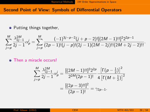
Putting things together,

M∑j=p

λ2M2j−1

2j − 1αjp =

M∑j=p

(−1)3j−p−2(j + p − 2)![(2M − 1)!!]222p−1

(2p − 1)!(j − p)!(2j − 1)(2M − 2j)!!(2M + 2j − 2)!!.

Then a miracle occurs!

M∑j=p

λ2M2j−1

2j − 1αjp =

[(2M − 1)!!]222p

22M(2p − 1)!

[Γ(p − 1

2 )]2

4[Γ(M + 1

2 )]2

=[(2p − 3)!!]2

(2p − 1)!= γ2p−1.



Series Convergence

Lemma

The series∑∞

p=1 γ2p−1 is convergent and its sum is π/2.

Proof.

The values γ2p−1 are simply the Taylor coefficients of sin−1(x).


Numerical Methods (2, 2M) Order Methods for Debye Polarization Models

Maxwell’s Equations in a Debye Media

Maxwell’s equations in a Debye medium can be written using the electricflux density D = ε∞E + P

∂B

∂t=∂E

∂z,

∂D

∂t=

1

µ0

∂B

∂z,

∂D

∂t+

1

τD = ε∞

∂E

∂t+εsτE


Numerical Methods (2, 2M) Order Methods for Debye Polarization Models

2− 2M Order Methods for Debye Media

Second order in time and 2Mth order in space schemes that arestaggered in both space and time. (Here h = ∆z)

Bn+ 1

2

j+ 12

− Bn− 1

2

j+ 12

∆t=

M∑p=1

λ2M2p−1

(2p − 1)∆z

(Enj+p − En

j−p+1

),

Dn+1j − Dn

j

∆t=

1

µ0

M∑p=1

λ2M2p−1

(2p − 1)∆z

(B

n+ 12

j+p−1/2 − Bn+ 1

2

j−p+1/2

),

Dn+1j − Dn

j

∆t+

1

τ

Dn+1j + Dn

j

2= ε∞

En+1j − En

j

∆t+εsτ

(En+1j + En

j

2

)


Numerical Methods von Neumann Stability Analysis

Stability Analysis: von Neumann Analysis

1 Linear models.

2 Analyze the models in the frequency domain.

3 Look for plane wave solution numerically evaluated at the discretespace-time point (tn, zj), or (tn+1/2, zj+1/2).

4 Assume a spatial dependence of the form

Bn+ 1

2

j+ 12

= Bn+ 12 (k)e

ikzj+ 1

2 ,

Enj = En(k)eikzj ,

Dnj = Dn(k)eikzj ,

k: wavenumber



Stability Analysis

1 Define the vector Un = [Bn− 12 , En, 1

ε0ε∞Dn]T .

2 We obtain the system Un+1 = AUn, where the amplification matrixA is

A =

1 −σ 0(

2 + hτ2 + hτηs

)σ∗

(2(1− q)− hτ (ηs + q)

2 + hτηs

) (2hτ

2 + hτηs

)σ∗ −q 1

,3

σ := −η∞∆zF(D(2M)

1,h

)= −2iν∞

M∑p=1

γ2p−1 sin2p−1

(k∆z

2

),

q := σσ∗ = |σ|2.



2− 2M Order Methods for Debye Media

The parameters c∞, ν∞, hτ and ηs are defined as

c2∞ := 1/(ε0µ0ε∞) = c2

0/ε∞,

ν∞ := (c∞∆t)/∆z ,

hτ := ∆t/τ,

ηs := εs/ε∞,

c0: Speed of light in vacuum

c∞: speed of light in the Debye medium.

ν∞: Courant (stability) number.

εs > ε∞ and τ > 0.



Stability Conditions

1 A scheme is stable ⇐⇒ the sequence (Un)n∈N is bounded.

2 Since A does not depend on time, then Un = AnU0, and stability isalso the boundedness of (An)n∈N.

3 If the eigenvalues of A, i.e., the roots of the CharacteristicPolynomial PD

(2,2M), lie outside the unit circle, then An growsexponentially and the scheme is unstable

4 If the eigenvalues of A, lie inside the unit circle, then limn→∞An = 0and the sequence is bounded.

5 The intermediate case may lead to different situations.



Characteristic Polynomial

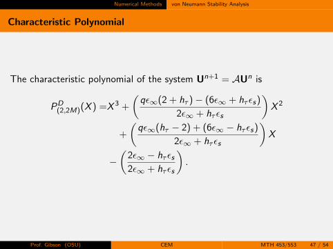
The characteristic polynomial of the system Un+1 = AUn is

PD(2,2M)(X ) =X 3 +

(qε∞(2 + hτ )− (6ε∞ + hτ εs)

2ε∞ + hτ εs

)X 2

+

(qε∞(hτ − 2) + (6ε∞ − hτ εs)

2ε∞ + hτ εs

)X

−(

2ε∞ − hτ εs2ε∞ + hτ εs

).



Stability Conditions

Theorem (Bokil-Gibson2011)

A necessary and sufficient stability condition for the (2, 2M) scheme forDebye is that q ∈ (0, 4), for all wavenumbers, k , i.e.,

4ν2∞

M∑p=1

γ2p−1 sin2p−1

(k∆z

2

)2

< 4, ∀k,

which implies that

ν∞

M∑p=1

γ2p−1

< 1⇐⇒ ν∞

M∑p=1

[(2p − 3)!!]2

(2p − 1)!

< 1.



Stability Bounds

For different values of M we obtain the following stability conditions

M = 1, ν∞ < 1⇐⇒ ∆t <∆z

c∞,

M = 2, ν∞

(1 +

1

6

)< 1⇐⇒ ∆t <

6∆z

7c∞,

M = 3, ν∞

(1 +

1

6+

3

40

)< 1⇐⇒ ∆t <

120∆z

149c∞,

...

M = M, ν∞

M∑p=1

γ2p−1

< 1⇐⇒ ∆t <∆z(∑M

p=1

[(2p − 3)!!]2

(2p − 1)!

)c∞

.



Stability Bounds

1 In the limiting case (as M →∞), we may evaluate the infinite seriesusing the convergence Lemma

2 Therefore,

M =∞, ν∞(π

2

)< 1⇐⇒ ∆t <

2∆z

π c∞.

3 The positivity of the coefficients γ2p−1 gives that the constraint on∆t is a lower bound on all constraints for any M. Therefore thisconstraint guarantees stability for all orders.



Other Details

1 This type of stability analysis can be applied to different polarizationmodels written as ODEs augmented to the Maxwell system, e.g.,Lorentz, Drude, multipole Debye, Lorentz media.

2 The second point of view also helps in obtaining closed fromnumerical dispersion relations for all (2, 2M) order schemes. See[Bokil-Gibson2011].


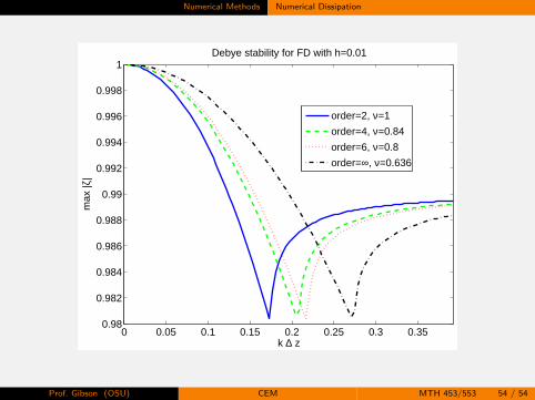
Numerical Methods Numerical Dissipation

We plot the maximum complex-time eigenvalue for the schemes. For thecontinuous model, this value should be one, thus the any difference is dueto numerical dissipation error.

Physical parameters:

ε∞ = 1

εs = 78.2

τ = 8.1× 10−12 sec.

These are appropriate constants for modeling water and are representativeof a large class of Debye type materials.



0 0.5 1 1.5 2 2.5 30.8

0.82

0.84

0.86

0.88

0.9

0.92

0.94

0.96

0.98

1

k ∆ z

Debye stability for FD with h=0.1

max

|ζ|

order=2, ν=1

order=4, ν=0.84

order=6, ν=0.8

order=∞, ν=0.636



0 0.05 0.1 0.15 0.2 0.25 0.3 0.350.98

0.982

0.984

0.986

0.988

0.99

0.992

0.994

0.996

0.998

1

k ∆ z

Debye stability for FD with h=0.01

max

|ζ|

order=2, ν=1

order=4, ν=0.84

order=6, ν=0.8

order=∞, ν=0.636


numerical methods for maxwell's equationsmath.oregonstate.edu/~gibsonn/553talk.pdf ·...

Documents