numerical methods in aerodynamics - aalborg · pdf filelid driven cavity flow, fortran...

Numerical Methods in AerodynamicsLecture 1: Basic Concepts of Fluid Flows

1

Plan for this course


2

Today's Lecture

Introduction to aerodynamicsNavier-Stokes equationsIntroduction to Fortran90Finite Volume method for solving differential equations

Example: diffusion problemExample: convection-diffusion problem

Exercise: Start solving the Navier Stokes equationsLid driven cavity flow, Fortran program


3

Literature


4

Why are we interested in knowing about aerodynamics?


5

Windturbine Aerodynamics


6

Navier-Stokes equations

Describe the fluid properties: velocity components, pressure, density, Internal energy and temperature.Can only be solved analytical for very simple problemsIn differential form the governing equations of the flow of a compressible Newtonian fluid are:

Mass equilibrium

Momentum equations

Energy equation

Unknowns: ρ, ui, p, I, T (7 unknowns, 5 equations).Equations of state: p =p(ρ, T) , I =I(ρ, T)


7

Incompressible, stationary flow

Density is constant

Mass equilibrium

Momentum equations

Unknowns: ui, p (4 unknowns, 4 equations).


8

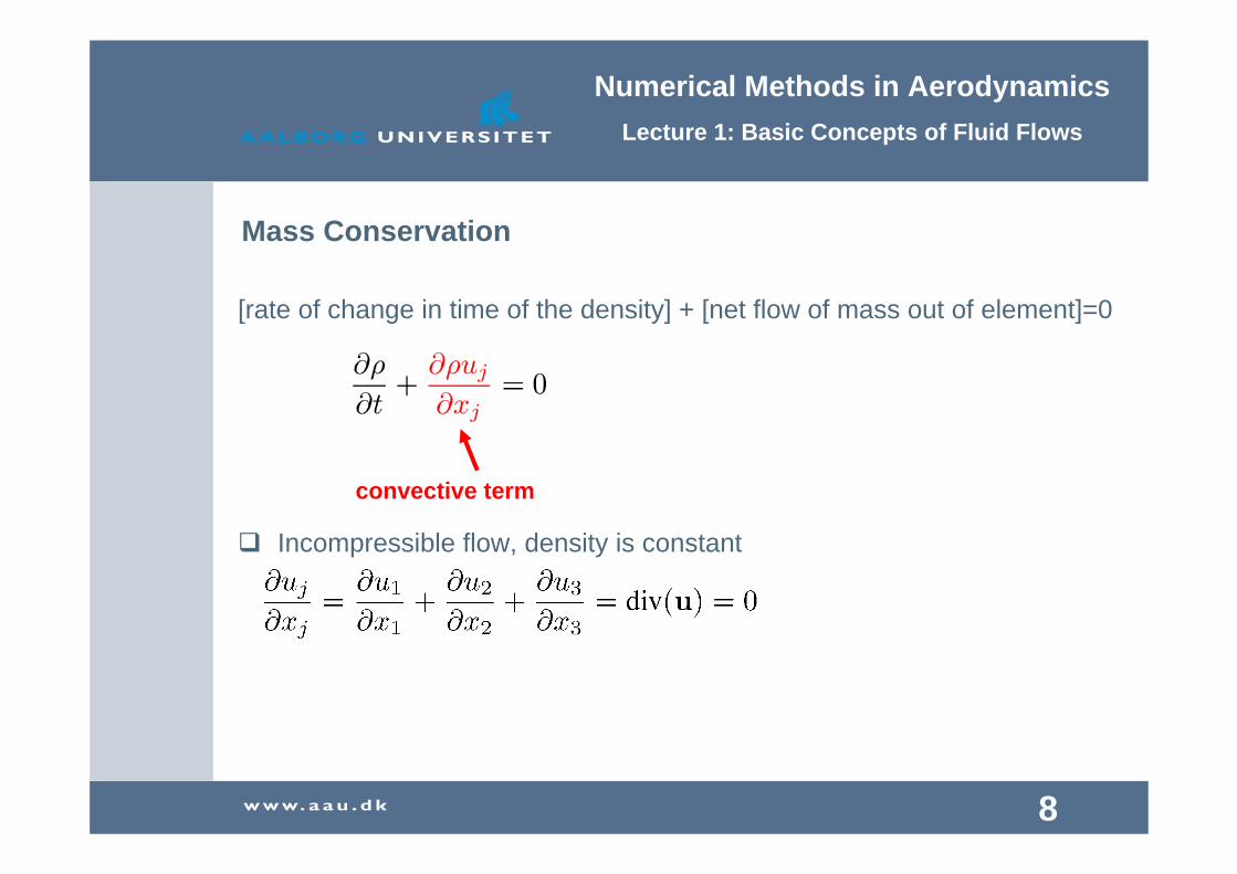
Mass Conservation

[rate of change in time of the density] + [net flow of mass out of element]=0

Incompressible flow, density is constant

convective term


9

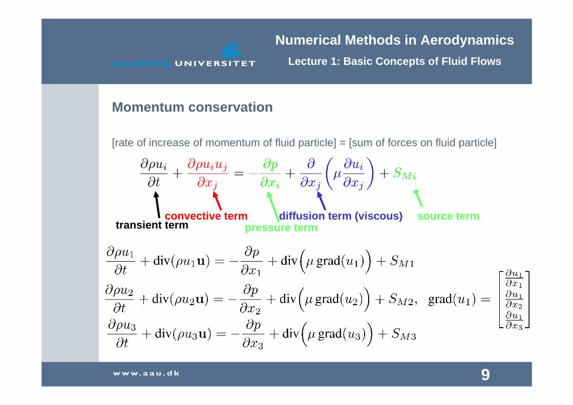
Momentum conservation

[rate of increase of momentum of fluid particle] = [sum of forces on fluid particle]

convective term diffusion term (viscous) source termpressure termtransient term


10

General transport equation

Mass conservation

Momentum conservation

Rate of increase of φin fluid element

+ Rate of flow of φ out of fluid element

Rate of increase of φ due to diffusion

+= Rate of increase of φdue to sources


11

Integral form of the general transport equation

Looking at a control volume (CV), stationary flow

Gauss' theorem

convective term diffusion term


12

BREAK

Next:Fortran90 programming


13

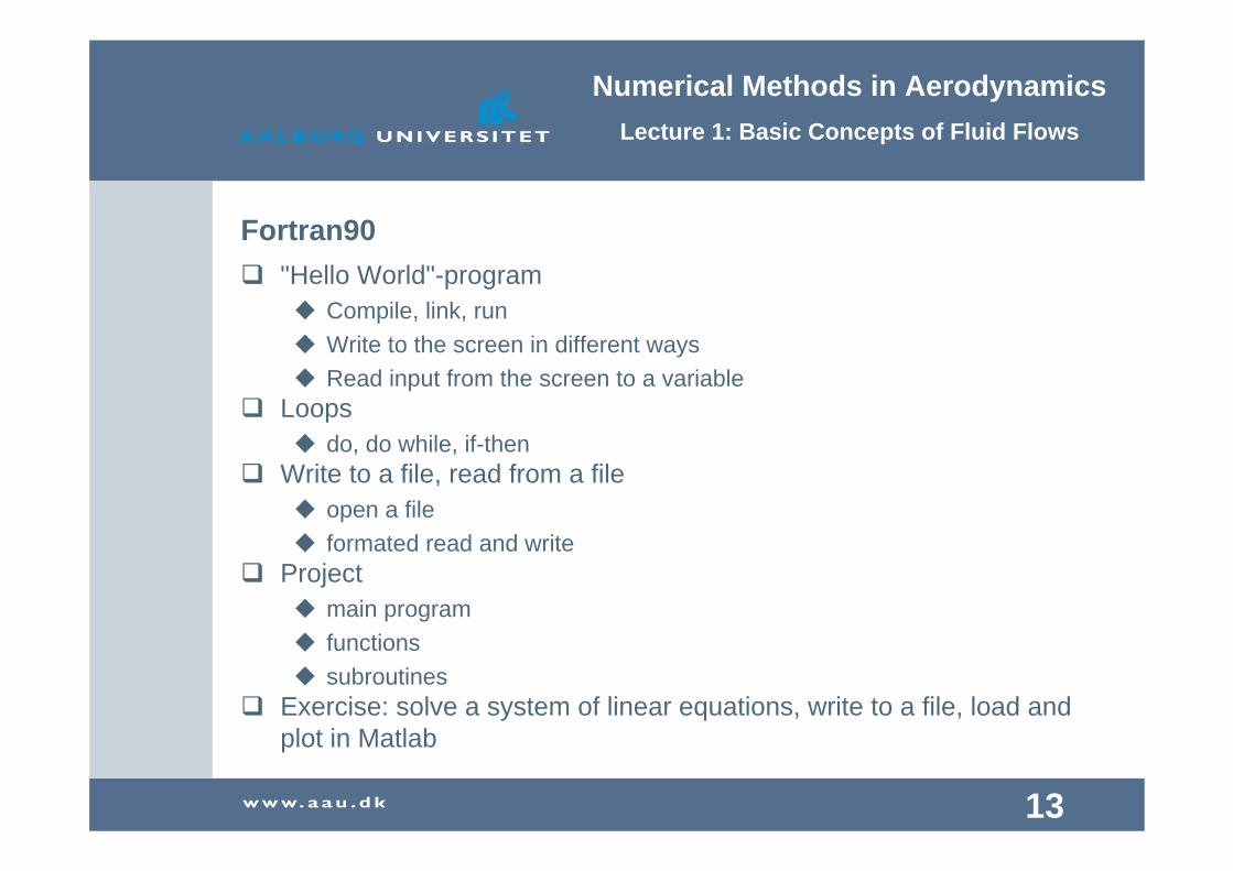
Fortran90 "Hello World"-program

Compile, link, runWrite to the screen in different waysRead input from the screen to a variable

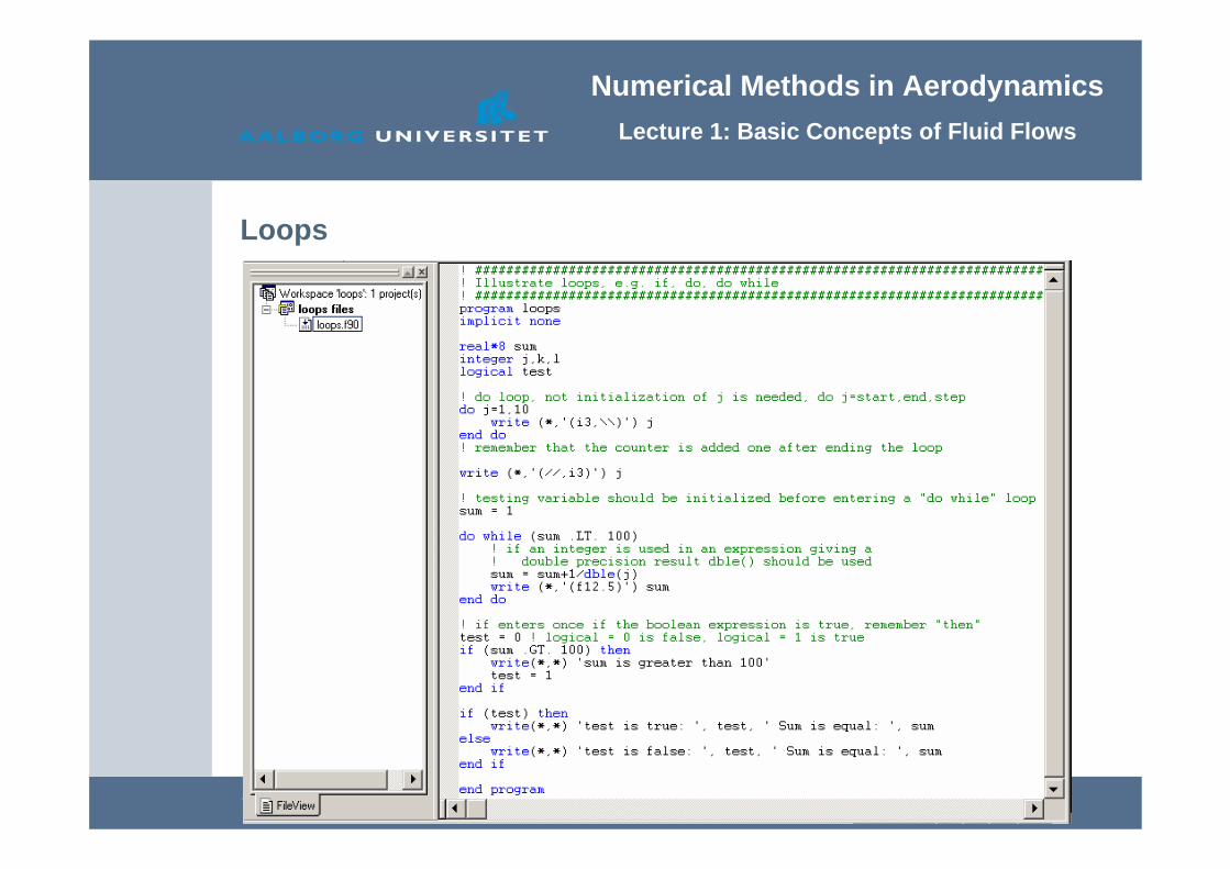
Loopsdo, do while, if-then

Write to a file, read from a fileopen a fileformated read and write

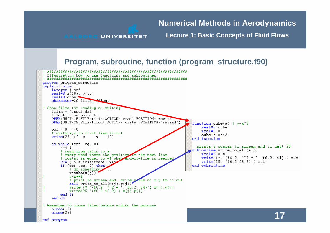
Projectmain programfunctionssubroutines

Exercise: solve a system of linear equations, write to a file, load and plot in Matlab


14

"Hello World"-program (hello_world.f90)


15

Loops


16

Read from text file and write to text file (write_file.f90)

Matlab code for loading a textfileplotting.m


17

Program, subroutine, function (program_structure.f90)


18

Exercise:Problem

solve the system of linear equations using an iterative method

write solution to a fileload and plot solution in Matlab


19

Exercise: Hint

You will need the following variablesinteger n,Ireal*8 Ta(5),Tb(5) ! Ta are the Tn values Tb are the Tn+1 values

Initial guess for TaTa = (/0,0,0,0,0/)


20

BREAK

Next: Finite-Volume method for solving differential equationsExample: diffusion problemExample: convection-diffusion problem


21

Steady state, diffusion problems

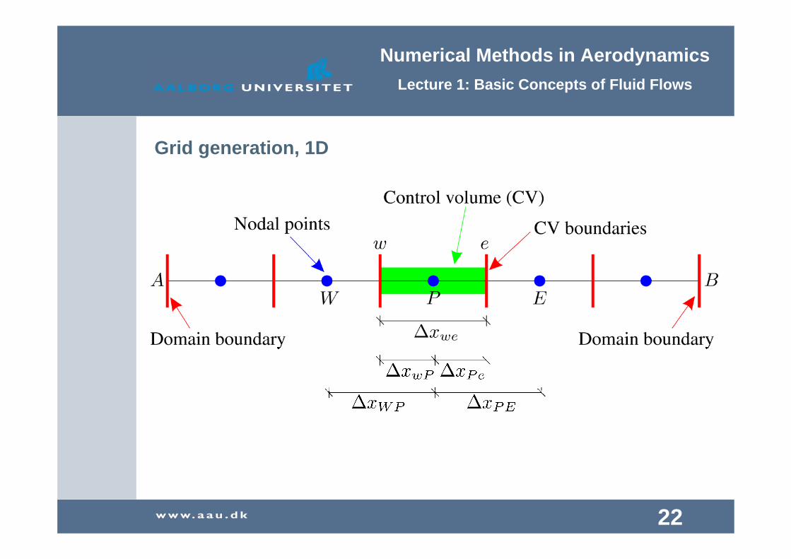
Grid generationDiscretisation of equationsSolution of the discretised equations


22

Grid generation, 1D


23

1D governing equation

Integral over CV and using Gauss' theorem

Out-going normal n

Solution to integral

Discretisation


24

Discretisation

The diffusive flux of φ entering the left-hand side (west) minus the diffusive flux leaving the right-hand side (east) is equal to the generation of φ

Central difference scheme for evaluating gradients

Inserting and rearranging


25

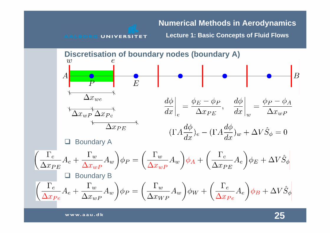
Discretisation of boundary nodes (boundary A)

Boundary A

Boundary B


26

Summary for the diffusion problem

Define Γ and A for all cell facesDefine the grid ∆xWP, ∆xPE, ∆xwP, ∆xPe for all control volumesInternal nodes

Boundary node A

Boundary node B


27

Solution of equations

The equations for each internal nodal point are set upThe equations for the boundary points are set up to incorporate the boundary conditionsThe system of linear equations can be put in matrix format

Various techniques may be used to solve the matrix equationDirect Methods:

Matrix inversionGaussian eliminationThomas algorithm or the tri-diagonal matrix algorithm (TDMA)

Indirect methods (iterative):Jacobi iteration (the one you used in the fortran exercise)Gauss-Seidel iteration


28

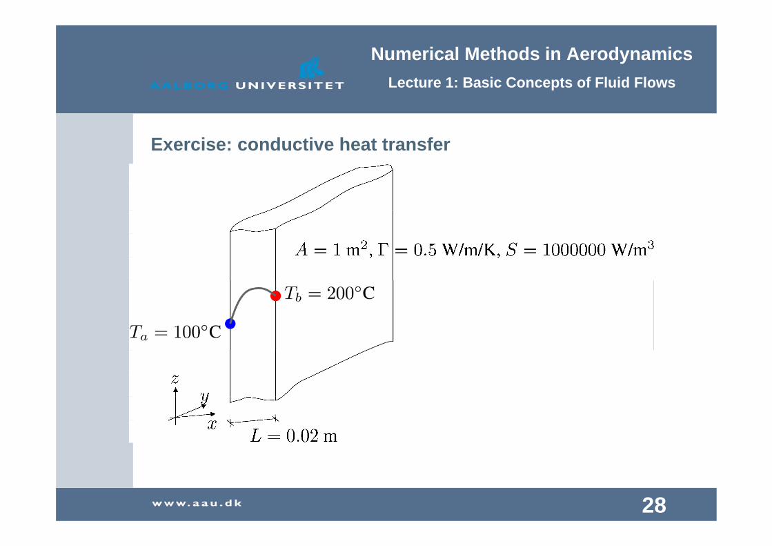
Exercise: conductive heat transfer


29

Grid

Set up the system of linear algebraic equations, use five CV's i.e. ∆x=0.004 m


30

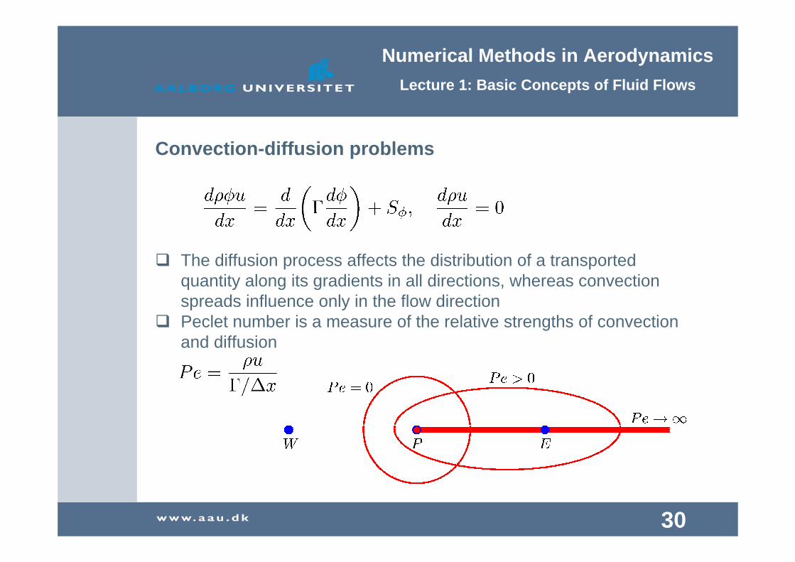
Convection-diffusion problems

The diffusion process affects the distribution of a transported quantity along its gradients in all directions, whereas convection spreads influence only in the flow directionPeclet number is a measure of the relative strengths of convection and diffusion


31

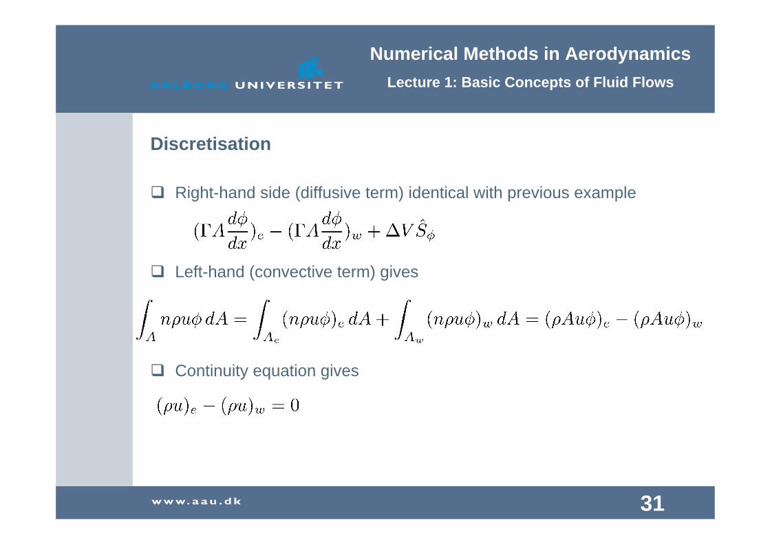
Discretisation

Right-hand side (diffusive term) identical with previous example

Left-hand (convective term) gives

Continuity equation gives


32

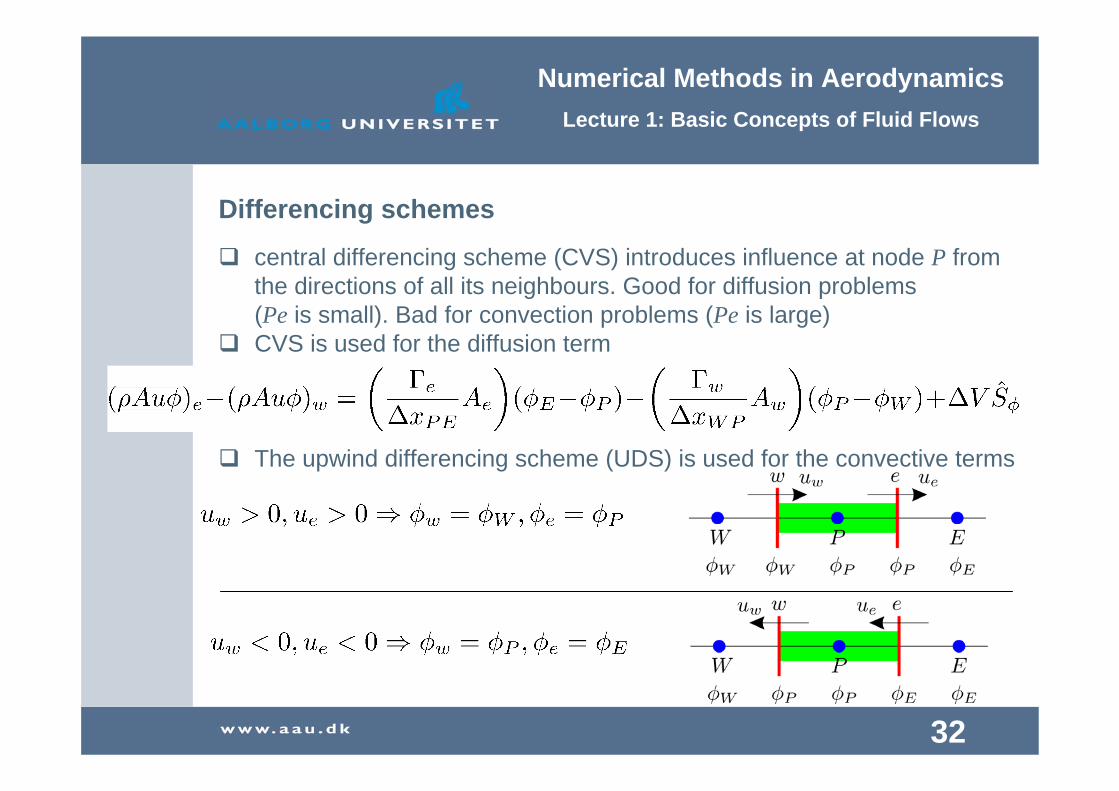
Differencing schemes

central differencing scheme (CVS) introduces influence at node P from the directions of all its neighbours. Good for diffusion problems (Pe is small). Bad for convection problems (Pe is large)CVS is used for the diffusion term

The upwind differencing scheme (UDS) is used for the convective terms


33

Differencing schemes internal points


34

Differencing schemes boundary points

Boundary node A

Boundary node B


35

Example: 1D transport of φ by convection and diffusion

Velocity is assumed known u=0.1 m/sNo source term S=0Area is constant Ae=Aw=ADensity is constant ρ=1Diffusion coefficient is constant Γ=0.1Grid L=1 m, ∆x=0.2 mPeclet number Pe = 0.2 Boundary φA=1, φB=0


36

Solution

Analytical solution


37

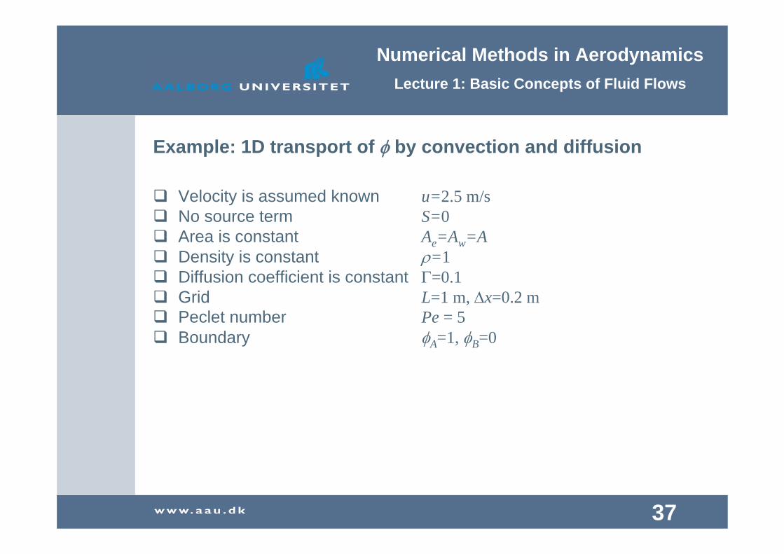
Example: 1D transport of φ by convection and diffusion

Velocity is assumed known u=2.5 m/sNo source term S=0Area is constant Ae=Aw=ADensity is constant ρ=1Diffusion coefficient is constant Γ=0.1Grid L=1 m, ∆x=0.2 mPeclet number Pe = 5 Boundary φA=1, φB=0


38

Solution

Analytical solution


39

Problems with UDS

Only first order accurate, where CDS is second order accurateIntroduces numerical diffusion. The leading truncation error term resembles a diffusive flux


40

Exercise: Setting up and running the flow solving program

Three parts existsGrid generation (post processing)Solution of the problem (solver)Plotting (pre processing)

Include these in one projectRun the grid programRun the solverRun the plotting program


41

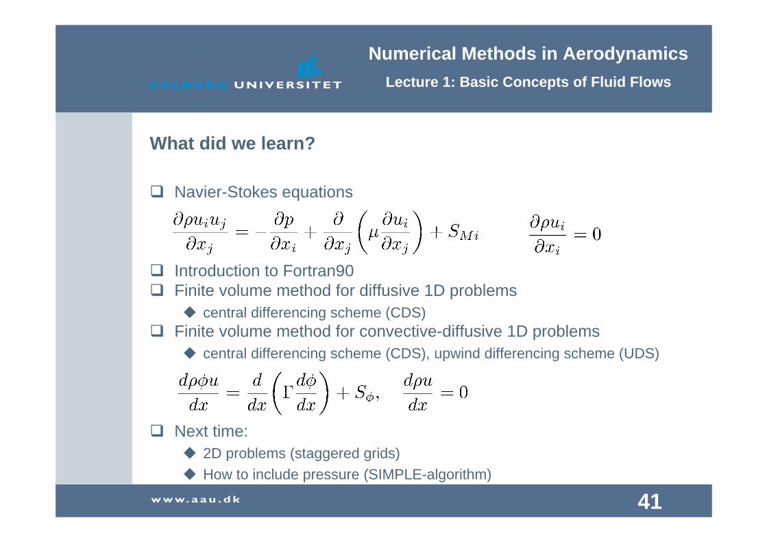
What did we learn?

Navier-Stokes equations

Introduction to Fortran90Finite volume method for diffusive 1D problems

central differencing scheme (CDS)Finite volume method for convective-diffusive 1D problems

central differencing scheme (CDS), upwind differencing scheme (UDS)

Next time:2D problems (staggered grids)How to include pressure (SIMPLE-algorithm)


42

Thank you for your attention

numerical methods in aerodynamics - aalborg · pdf filelid driven cavity flow, fortran...

Documents