numerical methods in civil engineering method.pdf · numerical differentiation and integration....

NUMERICAL METHODS IN CIVIL ENGINEERING

LECTURE NOTES

Janusz ORKISZ

2007-09-09

Search ON Google "EME Technologies"

l.888 Numerical Methods in Civil Engineering I Introduction, errors in numerical analysis. Solution of nonlinear algebraic equations Solution of large systems of linear algebraic equations by direct and iterative methods. Introduction to matrix eigenvalue problems. Examples are drawn from structural mechanics. Prep. Admission to Graduate School of Engineering. l.889 Numerical Methods in Civil Engineering II

Continuation of l.888. Approximation of functions: interpolation, and least squares curve fitting; orthogonal polynomials. Numerical differentiation and integration. Solution of ordinary and partial differential equations, and integral equations; discrete methods of solution of initial and boundary-value problems. Examples are drawn from structural mechanics, geotechnical engineering, hydrology and hydraulics. Prep. l.888, Numerical Methods in Civil Engineering I.


Table of contents

1. Introduction

1.1. Numerical method 1.2. Errors in numerical computation 1.3. Significant digits 1.4. Number representation 1.5. Error bounds 1.6. Convergence 1.7. Stability

2. Solution of non-linear algebraic equation

2.1. Introduction 2.2. The method of simple iterations

2.2.1. Algorithm 2.2.2. Convergence theorems 2.2.3. Iterative solution criteria 2.2.4. Acceleration of convergence by the relaxation technique

2.3. Newton – Raphson method 2.3.1. Algorithm 2.3.2. Convergence criteria 2.3.3. Relaxation approach to the Newton – Raphson method 2.3.4. Modification for multiple routs

2.4. The secant method 2.5. Regula falsi 2.6. General remarks

3. Vector and matrix norm

3.1. Vector norm 3.2. Matrix norm

4. Systems of nonlinear equations

4.1. The method of simple iterations 4.2. Newton – Raphson method

5. Solution of simultaneous linear algebraic equations (SLAE)

5.1. Introduction 5.2. Gaussian elimination 5.3. Matrix factorization LU 5.4. Choleski elimination method 5.5. Iterative methods 5.6. Matrix factorization LU by the Gaussian Elimination 5.7. Matrix inversion

5.7.1. Inversion of squared matrix using Gaussian Elimination


5.7.2. Inversion of the lower triangular matrix 5.8. Overdetermined simultaneous linear equations

6. The algebraic eigenvalue problem

6.1. Introduction 6.2. Classification of numerical solution methods 6.3. Theorems 6.4. The power method

6.4.1. Concept of the method and its convergence 6.4.2. Procedure using the Rayleigh quotient 6.4.3. Shift of the eigenspectrum 6.4.4. Application of shift to acceleration of convergence to max 1λ λ= 6.4.5. Application of a shift to acceleration of convergence to λmin

6.5. Inverse iteration method 6.5.1. The basic algorithm 6.5.2. Use of inverse and shift In order to find the eigenvalue closest to a given one

6.6. The generalized eigenvalue problem 6.7. The Jacobi method

6.7.1. Conditions imposed on transformation

7. Ill-conditioned systems of simultaneous linear equations

7.1. Introduction 7.2. Solution approach

8. Approximation

8.1. Introduction 8.2. Interpolation in 1D space 8.3. Lagrangian Interpolation ( 1D Approximation) 8.4. Inverse Lagrangian Interpolation 8.5. Chebychev polynomials 8.6. Hermite Interpolation 8.7. Interpolation by spline functions

8.7.1. Introduction 8.7.2. Definition 8.7.3. Extra conditions

8.8. The Best approximation 8.9. Least squares approach 8.10. Inner Product 8.11. The generation of orthogonal functions by GRAM - SCHMIDT process

8.11.1. Orthonormalization 8.11.2. Weighted orthogonalization 8.11.3. Weighted orthonormalization

8.12. Approximation in a 2D domain 8.12.1. Lagrangian approximation over rectangular domain


9. Numerical differentation

9.1. By means of the approximation and differentation 9.2. Generation of numerical derivatives by undetermined coefficients method

10. Numerical integration

10.1. Introduction 10.2. Newton – Cotes formulas

10.2.1. Composite rules 10.3. Gaussian quadrature

10.3.1. Composite Gaussian – Legendre integration 10.3.2. Composite Gaussian – Legendre integration 10.3.3. Summary of the Gaussian integration 10.3.4. Special topics

11. Numerical solution of ordinary differential equations

11.1. Introduction 11.2. Classification 11.3. Numerical approach 11.4. The Euler Method 11.5. Runge Kutta method 11.6. Multistep formulas

11.6.1. Open (Explicit) (Adams – Bashforth) formulas 11.6.2. Closed (Implicit) formulas (Adams – Moulton) 11.6.3. Predictor – corrector method

12. Boundary value problems

12.1. Finite difference solution approach

13. On solution of boundary value problems for partial differential equations by the finite difference approach (FDM)

13.1. Formulation 13.2. Classification of the second order problems 13.3. Solution approach for solution of elliptic equations by FDM

14. Parabolic equations

15. Hyperbolic equations

16. MFDM

16.1. MWLS Approximation


Chapter 1—1/6 2007-11-05

11.. IINNTTRROODDUUCCTTIIOONN

1.1. NUMERICAL METHOD

− any method that uses only four basic arithmetic operations : + , − , : , ∗ − theory and art.

x = a → x a2 = , 0a ≥

xax

= , 0x ≠

x x xax

+ = +

x xax

= +⎛⎝⎜

⎞⎠⎟

12

− numerical method

⎟⎟⎠

⎞⎜⎜⎝

⎛+=

−−

112

1

nnn x

axx

1.2. ERRORS IN NUMERICAL COMPUTATION

Types of errors : Inevitable error

(i) Error arising from the inadequacy of the mathematical model

Example :

Pendulum

l

j

R

mg

ma


Chapter 1—2/6 2007-11-05

a lddt

=2

2ϕ

- acceleration

2

2 sin 0nd d g

dt dt lϕ ϕα ⎛ ⎞+ +⎜ ⎟

⎝ ⎠ϕ = - nonlinear model including large displacements

and friction

ddt

gl

2

2 0ϕ

ϕ+ = - simplified model - small displacement,

linearized equation and no friction

(ii) Error noise in the input data

, g , l ( )ϕ 0 , dd t t

ϕ= 0

, ..........

Error of a solution method

Example:

( , ( ))d f t tdtϕ ϕ=

Euler method

t

j

Exact solution


Chapter 1—3/6 2007-11-05

Numerical errors

(iii) Errors due to series truncation

Example

The temperature in a thin bar: (u x t, )

( ) ( )2 2 10

21 1

, exp sinnn n

n t n xu x t Cl lπ π∞ ∞

= =

−= = +∑ ∑

11n=∑

10

1n=

≈ ∑

(iv) Round off error

Example

x = =23

0 667.

THE OTHER CLASSIFICATION OF ERRORS

(i) The absolute error

Let x - exact value, x% - approximate value ε = −~x x

(ii) The relative error

δ =−~x xx

PRESENTATION OF RESULTS

( )expected 1 x x xε δ= ± = ±% %

Example

( )expected 2.53 0.10 2.53 1 0.04 2.53 4%x = ± ≈ ± = ±


Chapter 1—4/6 2007-11-05

1.3. SIGNIFICANT DIGITS

Number of digits starting from the first non-zero on the left side

Example

Number of significant digits

Number of significant digits

2345000 7 5 1 2.345000 7 5.0 2 0.023450 5 5.000 4 0.02345 4

Example

Subtraction Number of significant digits

2.3485302 8 -2.3485280 8

0.0000022 2

1.4. NUMBER REPRESENTATION

FIXED POINT FLOATING POINT 324.2500 : 1000 324.2500 = 3.2425 ×102 : 103

.3242 : 100 3.2425 ×10-1 : 102

.0032 : 10 3.2425 × 10-3 : 10 .0003 3.2425 × 10-4

1.5. ERROR BOUNDS

(iii) Summation and subtraction

Given: ,a a b± ∆ ± ∆b Searched: x a b a a b= + = ± ∆ + ± ∆b error evaluation

x x a b a b∆ = − − ≤ ∆ + ∆

(iv) Multiplication and division

ln ln ln ln lnabx x a b ccf

= → = + − − f

dx da db dc dfx a b c f

= + − −

error evaluation

a b c fx xa b c f

⎛ ⎞∆ ∆ ∆ ∆∆ ≤ + + +⎜ ⎟

⎝ ⎠


Chapter 1—5/6 2007-11-05

1.6. CONVERGENCE

Example

11

12n n

n

ax xx−

−

⎛ ⎞= +⎜

⎝ ⎠⎟ , ?lim =

∞→nnx

let

( ) 1 nn n

x x x xx nδ δ−

= → = +

( ) ( ) ( )11

1 1 1 2 1n n

n

ax xx

δ δδ−

−

⎡ ⎤+ = + +⎢ ⎥+⎣ ⎦ x

a⋅

1 1

1 11 1

21

1

11 1 11 1 1 2 1 2 1

1 2 2 1

n nn n n

n n

n

n

δ δδ δ δδ δ

δδ

− −− −

− −

−

−

⎡ ⎤ ⎡ + −+ = + + = + + =⎢ ⎥ ⎢+ +⎣ ⎦ ⎣

⎛ ⎞= +⎜ ⎟+⎝ ⎠

⎤⎥⎦

for

10 0 1

1

0 0 11

nn

n

x a δδ δδ−

−−

= → > → > → <+

one obtaines

( )

21 1

1 11 1

1 1 2 1 2 1 2

n nn n

n n

δ δnδ δ δ

δ δ− −

− −− −

= = <+ +

11 2n nδ δ −< → iteration is convergent

lim 0 limn nn n

x aδ→∞ →∞

= → →

In numerical calculations we deal with a number N. It describes a term that satisfy an admissible error B requirement where

n Bε < for , where n N≥

( ) ( )( )

11 11 1

1 1n nn n n n

nn n

x xx xx x

δ δ

n

δ δεδ δ

−− −+ − +− −= = =

+ +


Chapter 6/6 2007-11-05

1.7. STABILITY

Solution is stable if it remains bounded despite truncation and round off errors. Let

( ) ( ) ( )2

11

1 1

= nn n n n n n n

n n

1 a 1x x 1 x 1 12 x 2 1

δnγ γ δ γ

δ−

−− −

⎛ ⎞= + + + → = + +⎜ ⎟ +⎝ ⎠

% %%

γ

nlim = nn

δ γ→∞

→ precision of the final result corresponds to the precision of

the last step of calculations i.e. ( ) nx x 1 γ→ +%

Example

Unstable calculations

(v) Time integration process

(vi) Ill-conditioned simultaneous algebraic equations

6Search ON Google "EME Technologies"

Chapter 2—1/15 2007-11-05

22.. SSOOLLUUTTIIOONN OOFF NNOONN--LLIINNEEAARR AALLGGEEBBRRAAIICC EEQQUUAATTIIOONNSS

2.1. INTRODUCTION

- source of algebraic equations - multiple roots - start from sketch - iteration methods

equation to be solved ( ) 0 ...y x x= → =

2.2. THE METHOD OF SIMPLE ITERATIONS

2.2.1. Algorithm Algorithm Example Let

x f x= ( ) 11

1 2n n

n

ax xx−

−

⎛ ⎞= +⎜ ⎟

⎝ ⎠ a=2, x0=2

( )x f x1 0= 11 2 32 1.50002 2 2

x ⎛ ⎞= + = =⎜ ⎟⎝ ⎠

( )x f x2 1= 21 3 2 172 1.41672 2 3 12

x ⎛ ⎞= + ⋅ = =⎜ ⎟⎝ ⎠

.................. .................. ( )x f xn n= −1

..................


Chapter 2—2/15 2007-11-05

Geometrical interpretation

Example :

2 4 2.3 0 ( )x x x− + = → = f x Algorithm

(i) (ii)

( ) ( )2

21

2.3 1 2.34 4n n

xx x x −

+= → = +

Let 0 0.6x =

14 2.3 4 2.3n nx x x x −= − → = −

( )21

1.6 2.3 .6654

x = + = 1 0.316x =

( )22

1.665 2.3 .6864

x = + = 2 1.264 2.3x = − ……………................ cannot be performed

( )26

1.696 2.3 .6964

x = + =

Solution converged within three digits :

6 5

6

0.696 0.696 00.696

x xx− −

= =


Chapter 2—3/15 2007-11-05

2.2.2. Convergence theorems Theorem 1

If ( ) ( )1 2 1 2f x f x L x x− ≤ − with 0 L 1< <

for [ ]1 2, , ;x x a b∈ then the equation ( )x f x= has at most one root in [ ],a b .

Theorem 2

If ( )f x satisfy conditions of Theorem 1 then the iterative method

( )x f xn n= −1 converges to the unique solution [ ], ;x a b∈ of ( )x f x= for any [ ]0 , ;x a b∈


2.2.3. Iterative solution criteria Convergence

1n nn

n

x x Bx

δ −−= <

Residuum

1 1 1

1

( )( )

n n n nn n

n n

f x x x xr Bf x x

δ− − −

−

− −= = = <

Notice : both criteria are the same for the simple iterations method


Chapter 2—4/15 2007-11-05

2.2.4. Acceleration of convergence by the relaxation technique

( )x f x=

( ) ( ) ( )11 1

x x x f x x x f x g xαα αα α

+ = + → = + ≡+ +

The best situation if ' ( ) 0g x ≈

( ) ( )1' '1 1

g x f xαα α

= ++ +

let ( ) ( )* *' 0 'g x f xα= → = −

then

( ) ( ) ( ) ( )( )

*

* *

'11 ' 1 '

f xg x f x x

f x f x= −

− −

Example :

( ) ( )22 1a a ax a 0 x f x f x

x x x′= > → = → = → = − = −

then

( ) ( ) ( )1 1 1

1 1 1 1 2a ag x x xx x

− ⎛ ⎞= − = ⎜ ⎟− − − − ⎝ ⎠+

hence

11

12n n

n

ax xx−

−

⎛ ⎞= +⎜ ⎟

⎝ ⎠


Chapter 2—5/15 2007-11-05

2.3. NEWTON – RAPHSON METHOD

2.3.1. Algorithm ( )F x = 0

2

22

1( ) ( ) ... ( ) '( ) ( ) '( ) 02x x

dF d FF x h F x h h F x F x h R F x F x hdx dx

+ = + + + = + + ≈ + =

( ) ( ) ( )( )

0 F x

F x F x h hF x

′+ = → = −′

( )( )

11 1

1

nn n n

n

F xx x h x

F x−

− −−

= + = −′


2.3.2. Convergence criteria Solution convergence

11

n nn

n

x x Bx

δ −−= <

Residuum

2 00

( ) , (( )

nn

F xr B F xF x

= < ) 0≠


Chapter 2—6/15 2007-11-05

Example

x

F

x0

x*

x1x2

y=x - 22

2 2 x 2 x 2= → − = 0 ( )F x x= −2 2, ( )′ =F x x2

x xx

xn nn

n= −

−−

−

−1

12

1

22

x0 2=

2

12 2 32 1.5000002 2 2

x −= − = =

⋅

94

2 32

23 17 1.4166672 2 12

x −= − = =

⋅

3577 1.414216408

x = =

……………………...

Convergence

32

1 32

2 0.333333δ −= =

( )232

1 2

20.125000

2 2r

−= =

−


Chapter 2—7/15 2007-11-05

17 312 2

2 1712

0.058824δ −= =

( )21712

2 2

20.003472

2 2r

−= =

−

577 17408 12

3 577408

0.001733δ−

= =

( )2577408

3 2

20.000003

2 2r

−= =

−

Convergence

-6-5-4-3-2-10

0 0,1 0,2 0,3 0,4 0,5 0,6

log10(no of iteration)

log1

0(d)

, log

10(r

)

solution convergence residuum convergence

2.3.3. Relaxation approach to the Newton – Raphson method ( )F x = 0

( ) ( ) ( ) 1x F x x x x F x g xα αα

+ = → = + ≡

( ) ( )′ = + ′g x F x11α

( ) ( )

*

1g x 0F x

α∗′ = → = −′

( )( )

F x

x xF x

= − →′

( )( )

11

1

nn n

n

F xx x

F x−

−−

= −′


Chapter 2—8/15 2007-11-05

2.3.4. Modification for multiple routs Let x c= be a root of multiplicity. ( )F xThen one way introduce

( ) ( )( ) ( ) ( ) ( )

( )( )2 F x F x F x

u x u x 1F x F x

′′′= → = −

′ ′ Instead to apply the Newton-Raphson method to ( )F x ( )u x

( )( )x x

u xu xn n

n

n

= −′−

−

−1

1

1

Example

100

-100

-200

y

x

2 4 6 8

4 3 2

3 2

2

F(x)= x - 8.6x - 35.51x 464.4x - 998.46 = 0F'(x)= 4x - 25.8x -71.02x+ 464.4F''(x)= 12x - 51.6x -71.02

+

Let x0 4 0= . ( )F 4 0 3 42. . ;= −

F'(4.0)= 23.52 ( )′′ = −F 4 0 85 42. .

( ) ( )( )

( ) ( ) ( )( )( )2 2

F 4.0 -3.42u 4 = = = -0.145408F 4.0 23.52

F 4.0 F'' 4.0 -3.42 (-85.42)u' 4 = 1.0 - = 1.0 - = 0.471906(23.52)F' 4.0

′

⋅ ⋅


Chapter 2—9/15 2007-11-05

( )( )x x

uu1 0

44

4 0145408

4719064 308129= −

′= −

−=.

..

.

x2 4 308129 00812 4 300001= − =. . . 3x 4.300000= methodRNalconvention −

x19 4 300000= . ………………………..........

2.4. THE SECANT METHOD

1 11 1 1

1 1

n nn n n n

n n

F xx x x FF F

− −− − −

− −

2

2

n

n

xF

−

−

−= − ≈ −

′ −

( )x xF

F Fx xn n

n

n nn n= −

−−−

−

− −− −1

1

1 21 2

starting points should satisfy the inequality

( ) ( )F x F x0 1 0< Geometrical interpretation

x

xF( )

x1

x3x2x0

x4

x5

x*

F0

F1


Chapter 2—10/15 2007-11-05

Example

x = 21x = 12

x = 00

xF( )

x =4 8134

x

x =3 34

Algorithm

( )x F x x2 22 2= → ≡ − = 0

2

2

Let

( )x F0 0 0= → = − and

( )x F1 2 2 4 2= → = − = then

222 (2 0

2 ( 2)x = − − =

− −) 1 − (1) 1F→ =

31 41 (1 2) 1.333333

1 2 3x −= − − = =

− − 4 2 0.222222

3 9F ⎛ ⎞→ = − = −⎜ ⎟⎝ ⎠

29

4 23

4 4 141 1.5555563 ( 1) 3 9

x − ⎛ ⎞= − − = =⎜ ⎟− − − ⎝ ⎠ 14 34 0.419753

9 81F ⎛ ⎞→ = =⎜ ⎟⎝ ⎠

( )3481

5 34 281 9

14 14 4 55 1.4102569 9 3 39

x ⎛ ⎞= − − = =⎜ ⎟− − ⎝ ⎠55 17 0.01117739 1521

F ⎛ ⎞→ = − = −⎜ ⎟⎝ ⎠

2 1.414214 true solutionTx = ≈ −


Chapter 2—11/15 2007-11-05

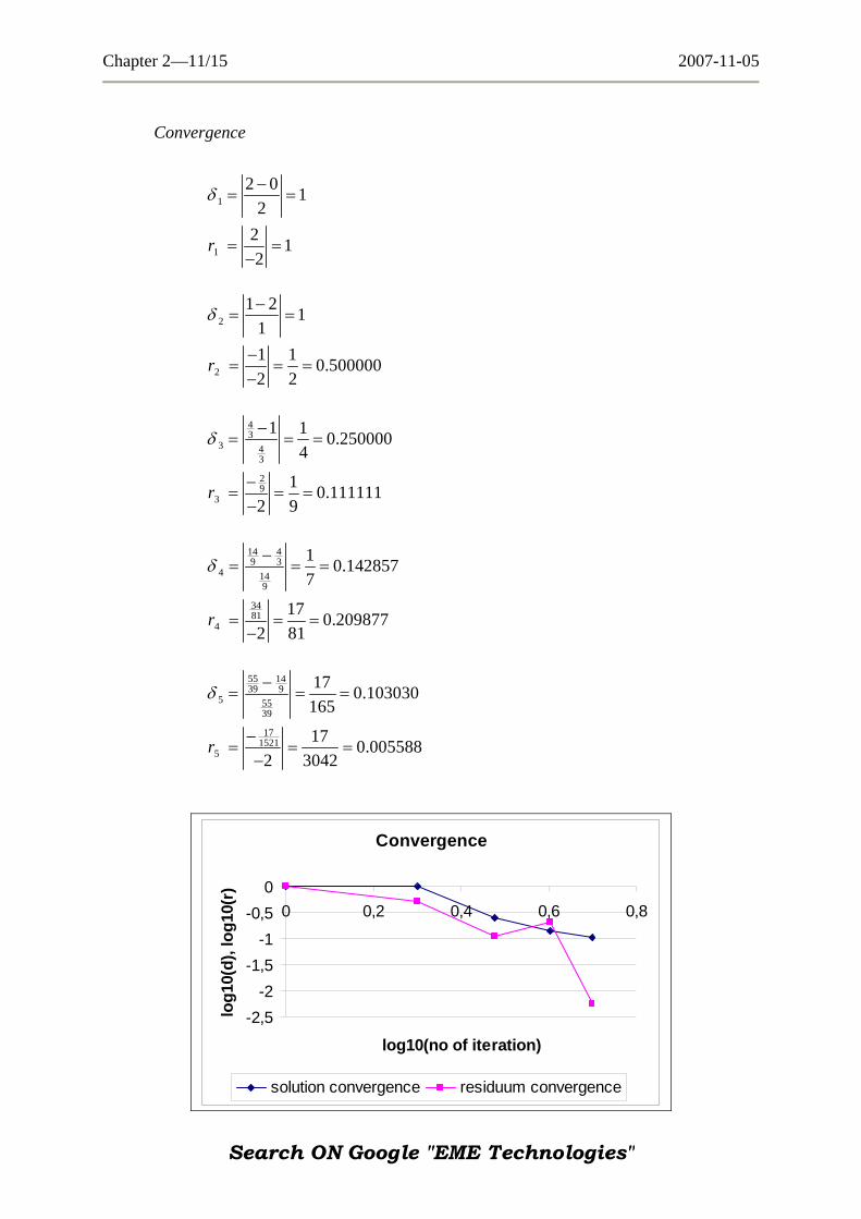
Convergence

1

1

2 0 12

2 12

r

δ −= =

= =−

2

2

1 2 111 1 0.5000002 2

r

δ −= =

−= = =−

43

3 43

29

3

1 1 0.2500004

1 0.1111112 9

r

δ −= = =

−= = =−

14 49 3

4 149

3481

4

1 0.1428577

17 0.2098772 81

r

δ −= = =

= = =−

55 1439 9

5 5539

171521

5

17 0.103030165

17 0.0055882 3042

r

δ −= = =

−= = =

−

Convergence

-2,5-2

-1,5-1

-0,50

0 0,2 0,4 0,6 0


log1

0(d)

, log

10(r

)

,8



Chapter 2—12/15 2007-11-05

2.5. REGULA FALSI

Let fix one starting point e.g. 0x x= in the secant method. Then 2 ,n n 2x F− − in the secant method are replaced by 0 0,x F .

(n-1n n-1 n-1 0

n-1 0

F )x = x - x - xF - F

, 0 1( ) ( ) 0F x F x <


Example

2 22 ( ) 2x F x x= → ≡ − = 0

2

2

Let ( )0 2 2x F= → = +and ( )1 0 0x F= → = −then

( ) ( )

( )

2

3

4

20 0 2 1 12 2

1 4 41 1 2 1.3333331 2 3 3 9

24 4 7 79 2 1.4000002

1

2

15 5 252

9

x F

−= − − = → = −

− −− ⎛ ⎞= − − = = → = −⎜ ⎟− − ⎝ ⎠

−⎛ ⎞ ⎛ ⎞= − − = = → = −⎜ ⎟ ⎜ ⎟⎝ ⎠ ⎝ ⎠− −

x F

x F

3 3


Chapter 2—13/15 2007-11-05

5

17 7 2425 2 1.41176915 5 172

252 ~ 1.414214 true solutionT

x = −

x

−⎛ ⎞− = =⎜ ⎟⎝ ⎠− −

= ≈ −

Convergence

1

1

0 2 not exist02r 1

2

δ −= →

−= =

21 0 1

1δ −

= = 21 1 0.500000

2 2r −= = =

43

3 43

1 1 0.2500004

δ −= = =

29

31 0.111111

2 9r −= = =

7 45 3

4 75

1 0.04761921

δ −= = =

4100

42 0.020000

2 100r −= = =

72417 5

5 2417

1 0.008333120

δ −= = =

2289

51 0.003460

2 289r −= = =

Convergence

-3-2,5

-2-1,5

-1-0,5

00 0,2 0,4 0,6 0,8


log1

0(d)

, log

10(r

)


Remarks

The regula falsi algorithm is more stable but slower than the one corresponding to the secant method.


Chapter 2—14/15 2007-11-05

2.6. GENERAL REMARKS

Rough preliminary evaluation of zeros (roots) is suggested

Traps Newton Raphson DIVERGENT (wrong starting point)

Secant Method DIVERGENT Regula Falsi CONVERGENT


Chapter 2—15/15 2007-11-05

Rough evaluation of solution methods

REGULA FALSI – the slowest but the safest SECANT METHOD – faster but less safe NEWTON-RAPHSON – the fastest but evaluation of the function

derivative is necessary


Chapter 3—1/2 2007-11-05

33.. VVEECCTTOORR AANNDD MMAATTRRIIXX NNOORRMM

Generalization of the modulus of a scalar function to a vector-valued function is called a vector norm, to a matrix-valued function is called a matrix norm.

3.1. VECTOR NORM

Vector norm x of the vector ∈x Vwhere: is a linear N-dimensional vector space, V α is a scalar satisfies the following conditions: (i) 0≥x ∀ ∈x V and 0=x if x = 0

(ii) α α= ⋅x x ∀ scalars α and ∀ ∈x V

(iii) + ≤ +x y x y ,∀ ∈x y V

Examples

(1)

122

11

N

ii

x=

⎡= ⎢⎣ ⎦∑x ⎤

⎥ p = 2 Euclidean norm

(2) 2

max iix=x p = ∞ maximum norm

(3)

1

31

N ppi

i

x=

⎡= ⎢⎣ ⎦∑x ⎤

⎥ 1p ≥

Examples

2,3,-6=x

( )1

12 2 2 22 +3 +6 =7=x

p = 2

2-6 = 6=x p = ∞

32 + 3 + -6 = 11=x p = 1


Chapter 3—2/2 2007-11-05

3.2. MATRIX NORM

Matrix norm of the ( matrix A must satisfy the following conditions: )N N× (i) 0≥A and 0=A if A = 0

(ii) α α= ⋅A A ∀ scalar α

(iii) + ≤ +A B A B

(iv) ≤ ⋅AB A B where and have to be of the same dimension. A B

Examples

12

21

1 1

N N

iji j

a= =

⎡ ⎤= ⎢ ⎥⎣ ⎦∑∑A or

12

21 2

1 1

1 N N

iji j

aN = =

⎡ ⎤= ⎢ ⎥⎣ ⎦

∑∑A - average value

21

maxN

iji j

a=

= ∑A or 2

1

1 maxN

iji j

aN =

= ∑A - maximum value

Example

1 2 34 5 67 8 9

⎡ ⎤⎢ ⎥= →⎢ ⎥⎢ ⎥⎣ ⎦

A

( )122 2 2 2 2 2 2 2 2

1 2

1 1 2 3 4 5 6 7 8 9 5.6273143⎡ ⎤= + + + + + + + + =⎢ ⎥⎣ ⎦

A

2

1 2 3 61 1max 4 5 6 max 15 83 3

7 8 9 24

⎧ + + ⎧⎪ ⎪= + + =⎨ ⎨⎪ ⎪+ + ⎩⎩

A =


Chapter 4—1/13 2007-11-05

44.. SSYYSSTTEEMMSS OOFF NNOONNLLIINNEEAARR EEQQUUAATTIIOONNSS

Denotations

1 2 3, , ,..., Nx x x x=x ( ) ( ) ( ) 1 ,...... NF F=F x x x ( ) =F x 0

Example

( )1

2

,

( , )

2

2 2

F x y y - 2x = 0

F x y x + y - 8 = 0

⎧ ≡⎪⎨

≡⎪⎩

4.1. THE METHOD OF SIMPLE ITERATIONS

Algorithm

( 1n n−=x f x ) 1( ), , ( )nf f=f x xK , 1, , nx x=x K Example

( )

( )

1

2

f

f

2

2

1x y2

y 8- x

⎧ = ≡⎪⎨⎪ = ≡⎩

x

x

,x y=x

( ) 2 21 y , 8 - x2

⎧ ⎫= ⎨ ⎬⎩ ⎭

f x

( )

( )

21

2

( )2 2

x y x f

y x + y + y - 8 f

⎧ = − ≡⎪ ⇒ =⎨= ≡⎪⎩

xx f x

x


Chapter 4—2/13 2007-11-05

Convergence criterion

1 ,n nn n

n

δ δ−−= ≤

x xx amdδ

amdδ - admissible error Theorem

Let ℜ denote the region a x bi i i i N= 1 2, , ,K, ≤ ≤ in the Euclidean N-dimensional space. Let f satisfy the conditions

– f is defined and continuous on ℜ – ( )f L 1≤ <J x

– For each , also lies in ∈ℜx ( )f x ℜ Then for any in ℜ the sequence of iterations 0x ( )1n n−=x f x is convergent to the

unique solution x

Jacobian matrix

1 1 1

1 2

1

n

N N

N

f f fx x x

f fx x

∂ ∂ ∂∂ ∂ ∂

∂ ∂∂ ∂

⎡ ⎤⎢ ⎥⎢ ⎥⎢ ⎥⎢ ⎥= ⎢ ⎥⎢ ⎥⎢ ⎥⎢ ⎥⎢ ⎥⎣ ⎦

J

L

L L

L L

L L

L L

Example

( )( )

21

2 22

f y x

f x y + y -

⎧ = −⎪⎨

= +⎪⎩

x

x 8 →

-1 2y2x 2y+1⎡ ⎤

= ⎢ ⎥⎣ ⎦

J

4.2. NEWTON – RAPHSON METHOD

( ) =F x 0

( ) ( ) ( ) ( )22

2

12

∂ ∂∂ ∂

+ = + + +F x F x

F x h F x h hx x

L

( ) ( ) ( ) ( ) ( ) 10∂∂

−+ ≈ + ≡ + = → = −F x

F x h F x h F x J x h h J Fx

1

1 1 1 1n n n n n n−

1− − − −= + = −x x h x J F −

n n n n

1 1 1− − −= −x x J F → 1 1 1 1n n n n n n 1− − − − −= − =J x J x F b


Chapter 4—3/13 2007-11-05

1 1n n n− −=J x b → Solution of simultaneous nx linear algebraic equations on each iteration step

lim nn→∞=x x

Relaxation factor µ may be also introduced

1 1 1n n n n n 1µ− − − −= −J x J x F

Example

y xx y

2

2 2

28

=

+ =

⎧⎨⎪

⎩⎪ →

2y - 2x = 0x y2 2 8 0+ − =

→ ( ) =F x

y xx y

2

2 2

28

−

+ −

⎧⎨⎪

⎩⎪

⎫⎬⎪

⎭⎪≡

( )( )

1

2

, F x

yF

⎧ ⎫ ⎧ ⎫⎪ ⎪ =⎨ ⎬ ⎨⎩ ⎭⎪ ⎪⎩ ⎭

xx

x⎬

1 1

2 2

-2 22 2

F Fyx y

JF F x yx y

∂ ∂⎡ ⎤⎢ ⎥∂ ∂ ⎡ ⎤⎢ ⎥= = ⎢ ⎥∂ ∂⎢ ⎥ ⎣ ⎦⎢ ⎥∂ ∂⎣ ⎦


Chapter 4—4/13 2007-11-05

Algorithm 2

2 21 1 1

2 2 2 2 22 2 2 2 8n n n n

y x y x y xx y y x y y x y

µ− − −

⎧ ⎫− −⎡ ⎤ ⎧ ⎫ ⎡ ⎤ ⎧ ⎫ −⎪ ⎪= −⎨ ⎬ ⎨ ⎬ ⎨ ⎬⎢ ⎥ ⎢ ⎥ + −⎪ ⎪⎣ ⎦ ⎩ ⎭ ⎣ ⎦ ⎩ ⎭ ⎩ ⎭

Let 1µ =

0

0 02.82842 2

x⎧ ⎫ ⎧ ⎫⎪ ⎪= =⎨ ⎬ ⎨⎪ ⎪ ⎩ ⎭⎩ ⎭

⎬

⎧ ⎫

⎩ ⎭

1

1

-2 5.65685 -2 5.65685 0 8-

0 5.65685 0 5.65685 2.8284 0xy

⎧ ⎫⎡ ⎤ ⎡ ⎤ ⎧ ⎫=⎨ ⎬ ⎨ ⎬ ⎨ ⎬⎢ ⎥ ⎢ ⎥

⎣ ⎦ ⎣ ⎦ ⎩ ⎭⎩ ⎭

1

4.00002.8284

x ⎧ ⎫= ⎨ ⎬⎩ ⎭

Error estimation

(after the first step of iteration)

Estimated relative solution error 1n nn

n

δ −−=

x xx

1 01

1

1 0 4.0000 0.0000, 2.8284 2.8284

4.0000 , 0.0000

δ−

=

− = − −

=

x xx

x x

Euclidean norm

( )( )

12

12

2 212

12 21

2

4.0000 0.0000 2.8284 0.81653.46414.0000 2.8284

Eδ⎡ ⎤+⎣ ⎦= =⎡ ⎤+⎣ ⎦

=

Maximum norm

1

sup 4.0000 , 0.0000 4.0000 1.0000sup 4.0000 ,2.8284 4.0000

Mδ = = =

Relative residual error 0

nnr =

FF

11

0

r =FF

Euclidean norm 1

2

21

1

( )n

jnEj

F=

⎧ ⎫= ⎨ ⎬⎩ ⎭∑F x


Chapter 4—5/13 2007-11-05

0

1

8.0000 , 0.0000

0.0000, 16.0000

=

=

F

F

( ) ( )

1 12 2

12

2 2 2 21 10 1 0 2 02 2

2 212

0.0000 8.0000 5.6568

0.0000 16.0000 11.3137

E

1 E

F F⎡ ⎤ ⎡ ⎤= + = + =⎣ ⎦⎣ ⎦

⎡ ⎤= + =⎣ ⎦

F x x

F

111.3137 2.00005.6568

Er = =

Maximum norm sup iM

iF=F

( )( )

0

1

1

sup 8.0000 , 0.0000 8.0000

sup 0.0000, 16.0000 16.0000

16.0000 2.00008.0000

M

M

Mr

= =

= =

= =

F

F

Brake-off test

Assume admissible errors for convergence CB and residuum RB ; check

61

61

81

81

0.81649658 10

1.00000000 10

2.00000000 10

2.00000000 10

EC

MC

ER

MR

B

B

r B

r B

δ

δ

−

−

−

−

= >

= >

= >

= >

=

=

=

=

⎫

⎭

Second step of iteration

2

2

-2.0000 5.6568 -2.0000 5.6568 4.0000 0.0000-

8.0000 5.6568 8.0000 5.6568 2.8284 16.0000xy

⎧ ⎫⎡ ⎤ ⎡ ⎤ ⎧ ⎫ ⎧=⎨ ⎬ ⎨ ⎬ ⎨ ⎬⎢ ⎥ ⎢ ⎥

⎣ ⎦ ⎣ ⎦ ⎩ ⎭ ⎩⎩ ⎭

2

2.40002.2627⎧ ⎫

= ⎨ ⎬⎩ ⎭

x

Error estimation (after the second step of iteration)

Estimated relative solution error

2 12

2

2 1 2.4000 4.0000 , 2.2627 2.8284 1.6000 , 0.5657

δ−

=

− = − − = − −

x xx

x x


Chapter 4—6/13 2007-11-05

Euclidean norm

( )( )

12

12

2 212

22 21

2

1.6000 0.5657 1.2000 0.51452.33242.4000 2.2627

Eδ⎡ ⎤+⎣ ⎦= =⎡ ⎤+⎣ ⎦

=

Maximum norm

2

sup 1.6000 , 0.5657 1.6000 0.6667sup 2.4000 , 2.2627 2.4000

Mδ = = =

Relative residual error

2

20

r =FF

Euclidean norm 1

2

21

1

( )n

jnEj

F=

⎧ ⎫= ⎨ ⎬⎩ ⎭∑F x

2 0.3200 , 2.8800=F

( ) ( ) ( )

11 22

12

22 2 21 10 1 0 2 02 2

2 212 2

0 2 2 5.6568

0.3200 2.8800 2.0490

E

E

F F ⎡ ⎤⎡ ⎤= + = + =⎣ ⎦ ⎢ ⎥⎣ ⎦

⎡ ⎤= + =⎣ ⎦

F x x

F

22.0490 0.36225.6568

Er = =

Maximum norm sup iM

iF=F

( )( )

0

2

2

sup 8.0000, 0.0000 8.0000

sup 0.3200 , 2.8800 2.8800

2.8800 0.36008.0000

M

M

Mr

= =

= =

= =

F

F

Brake-off test

62

62

82

82

0.51449576 10

0.66666667 10

0.36221541 10

0.36000000 10

EC

MC

ER

MR

B

B

r B

r B

δ

δ

−

−

−

−

= >

= >

= >

= >

=

=

=

=


Chapter 4—7/13 2007-11-05

Third step of iteration

⎫

⎭3

3

-2 4.5255 -2 4.5255 2.4000 0.3200 5.1200-

4.8 4.5255 4.8 4.5255 2.2627 2.8800 18.8800xy

⎧ ⎫⎡ ⎤ ⎡ ⎤ ⎧ ⎫ ⎧ ⎫ ⎧= =⎨ ⎬ ⎨ ⎬ ⎨ ⎬ ⎨ ⎬⎢ ⎥ ⎢ ⎥

⎣ ⎦ ⎣ ⎦ ⎩ ⎭ ⎩ ⎭ ⎩⎩ ⎭

3

2.02352.0257

x ⎧ ⎫= ⎨ ⎬⎩ ⎭

Error estimation

(after five steps of iteration)


3 23

3

3 2 2.0235 2.4000 , 2.0257 2.2627 0.3765 , 0.2371

δ−

=

− = − − = − −

x xx

x x

Euclidean norm

( )( )

12

12

2 212

32 21

2

0.3765 0.2371 0.3146 0.15542.02592.0235 2.0257

Eδ⎡ ⎤+⎣ ⎦= =⎡ ⎤+⎣ ⎦

=

Maximum norm

3

sup 0.3765 , 0.2371 0.3765 0.1859sup 2.0235 , 2.0257 2.0257

Mδ = = =


33

0

r =FF

Euclidean norm 1

2

21

1

( )n

jnEj

F=

⎧ ⎫= ⎨ ⎬⎩ ⎭∑F x

3 0.0562 , 0.1979= +F

( ) ( ) ( )

1 12 2

12

2 2 221 10 1 0 2 02 2

2 213 2

0.0000 8.0000 5.6568

0.0562 0.1979 0.1455

E

E

F F⎡ ⎤ ⎡ ⎤= + = + =⎣ ⎦ ⎣ ⎦

⎡ ⎤= + =⎣ ⎦

F x x

F

30.1455 0.02575.6568

Er = =


Chapter 4—8/13 2007-11-05

Maximum norm sup iMi

F=F

( )( )

0

3

3

sup 8.0000 , 0.0000 8.0000

sup 0.0562 , 0.1979 0.1979

0.1979 0.02478.0

M

M

Mr

= =

= =

= =

F

F

Brake-off test

63

63

83

83

0.15538736 10

0.18585147 10

0.02572098 10

0.02474265 10

EC

MC

ER

MR

B

B

r B

r B

δ

δ

−

−

−

−

= >

= >

= >

= >

=

=

=

=

⎫

⎭

Fourth step of iteration

4

4

-2 4.0513 -2 4.0513 2.0235 0.0562 4.1033-

4.0471 4.0513 4.0471 4.0513 2.0257 0.1979 16.1979xy

⎧ ⎫⎡ ⎤ ⎡ ⎤ ⎧ ⎫ ⎧ ⎫ ⎧= =⎨ ⎬ ⎨ ⎬ ⎨ ⎬ ⎨ ⎬⎢ ⎥ ⎢ ⎥

⎣ ⎦ ⎣ ⎦ ⎩ ⎭ ⎩ ⎭ ⎩⎩ ⎭

4

2.00012.0002

x ⎧ ⎫= ⎨ ⎬⎩ ⎭

Error estimation

(after four steps of iteration)

Estimated solution error

4 34

4

4 3 2.0001 2.0235 , 2.0002 2.0257 0.0236 , 0.0254

δ−

=

− = − − = − −

x xx

x x

Euclidean norm

( )( )

12

12

2 212

42 21

2

0.0234 0.0254 0.0247 0.01222.00022.0001 2.0002

Eδ⎡ ⎤+⎣ ⎦= =⎡ ⎤+⎣ ⎦

=

Maximum norm

4

sup 0.0234 , 0.0254 0.0254 0.0127sup 2.0001, 2.0002 2.0002

Mδ = = =


Chapter 4—9/13 2007-11-05


40

r =FF

Euclidean norm 1

2

21

1

( )n

jnEj

F=

⎧ ⎫= ⎨ ⎬⎩ ⎭∑F x

4 0.0007 , 0.0012= +F

( ) ( ) ( )

1 12 2

12

2 2 221 10 1 0 2 02 2

2 214 2

0.0000 8.0000 5.6568

0.0007 0.0012 0.0010

E

E

F F⎡ ⎤ ⎡ ⎤= + = + =⎣ ⎦ ⎣ ⎦

⎡ ⎤= + =⎣ ⎦

F x x

F

40.0010 0.00025.6568

Er = =

Maximum norm sup iM

iF=F

( )( )

0

4

4

sup 8.0000 , 0.0000 8.0000

sup 0.0007 , 0.0012 0.0012

0.0012 0.00028

M

M

Mr

= =

= =

= =

F

F

Brake-off test

64

64

84

84

0.01223018 10

0.01272134 10

0.00017009 10

0.0001460 10

EC

MC

ER

MR

B

B

r B

r B

δ

δ

−

−

−

−

= >

= >

= >

= >

=

=

=

=


Chapter 4—10/13 2007-11-05

Aitken acceleration process

( )x x x xn n n− = − −α 1

ASSUME α αn = constant

then

( )x x x xn n− = − −α 1

( )x x x xn n− = −− −1 2α 1

1 2

n n

n n

x x x xx x x x

−

− −

− −→ = →

− −

21

212

2 −−

−−

+−−

=nnn

nnn

xxxxxx

x

Example

2 22 4 3

44 3 2

2.400 2.0001 2.0235 1.99852 2.0001 2 2.0235 2.400

OLDNEW

OLD

x x xxx x x

− × −= = =

− + − × +

2 2

2 4 34

4 3 2

2.2627 2.0002 2.0257 1.99722 2.0002 2 2.0257 2.2627

OLDNEW

OLD

y y yyy y y

− × −= = =

− + − × +

Hence continuing N R− iteration

5

5

-2 3.9943 -2 3.9943 1.9985 -0.0085 3.9886-

3.9971 3.9943 3.9971 3.9943 1.9972 -0.0173 15.9828xy

⎧ ⎫⎡ ⎤ ⎡ ⎤ ⎧ ⎫ ⎧ ⎫ ⎧= =⎨ ⎬ ⎨ ⎬ ⎨ ⎬ ⎨ ⎬⎢ ⎥ ⎢ ⎥

⎣ ⎦ ⎣ ⎦ ⎩ ⎭ ⎩ ⎭ ⎩⎩ ⎭

⎫

⎭

5

2.00002.0000

x ⎧ ⎫= ⎨ ⎬⎩ ⎭


Chapter 4—11/13 2007-11-05

Error estimation

(after five steps of iteration)

Estimated solution error

5 45

5

5 4 2.0000 1.9985 , 2.0000 1.9972 0.0015 , 0.0028

δ−

=

− = − − =

x xx

x x

Euclidean norm

( )( )

12

12

2 212

52 21

2

0.0015 0.0028 0.0023 0.00112.00002.0000 2.0000

Eδ⎡ ⎤+⎣ ⎦= =⎡ ⎤+⎣ ⎦

=

Maximum norm

5

sup 0.0015 , 0.0028 0.0028 0.0014sup 2.0000 , 2.0000 2.0000

Mδ = = =


50

r =FF

Euclidean norm 1

2

21

1

( )n

jnEj

F=

⎧ ⎫= ⎨ ⎬⎩ ⎭∑F x

5 0.00001 , 0.00001=F

( ) ( ) ( )

1 12 2

12

2 2 221 10 1 0 2 02 2

2 215 2

0.0000 8.0000 5.6568

0.00001 0.00001 0.00001

E

E

F F⎡ ⎤ ⎡ ⎤= + = + =⎣ ⎦ ⎣ ⎦

⎡ ⎤= + =⎣ ⎦

F x x

F

50.00001 0.0000025.6568

Er = =

Maximum norm sup iM

iF=F

( )( )

0

5

5

sup 8.0000 , 0.0000 8.0000

sup 0.00001 , 0.00001 0.00001

0.00001 0.0000028.0000

M

M

Mr

= =

= =

= =

F

F


Chapter 4—12/13 2007-11-05

Brake-off test 6

56

5

85

85

0.00113413 10

0.00142690 10

0.00000164 10

0.00000129 10

EC

MC

ER

MR

B

B

r B

r B

δ

δ

−

−

−

−

= >

= >

= >

= >

=

=

=

=

SOLUTION SUMMARY Standard case – no acceleration

solution Relative solution error Relative residual error Iteration Number x y Euclidean

norm δEMaximum norm δM

Euclidean norm rE

Maximum norm rM

1 4.0000000000 2.8284271247 0.8164965809 1.0000000000 2.0000000000 2.0000000000 2 2.4000000000 2.2627416998 0.5144957554 0.6666666667 0.3622154055 0.3600000000 3 2.0235294118 2.0256529555 0.1553873552 0.1858514743 0.0257209770 0.0247426471 4 2.0000915541 2.0002076324 0.0122301810 0.0127213409 0.0001700889 0.0001495997 5 2.0000000014 2.0000000115 0.0000802250 0.0001038105 0.0000000084 0.0000000064 6 2.0000000000 2.0000000000 0.0000000041 0.0000000057 0.0000000000 0.0000000000

Aitken Acceleration included from the fourth iteration

solution Relative solution error Relative residual error Iteration Number x y Euclidean

norm δEMaximum norm δM

Euclidean norm rE

Maximum norm rM

1 4.0000000000 2.8284271247 0.8164965809 1.0000000000 2.0000000000 2.0000000000 2 2.4000000000 2.2627416998 0.5144957554 0.6666666667 0.3622154055 0.3600000000 3 2.0235294118 2.0256529555 0.1553873552 0.1858514743 0.0257209770 0.0247426471 4 1.9985355138 1.9971484092 0.0134178544 0.0142627172 0.0024025701 0.0021567540 5 2.0000003576 2.0000022149 0.0011341275 0.0014269013 0.0000016404 0.0000012862 6 2.0000000000 2.0000000000 0.0000007932 0.0000011074 0.0000000000 0.0000000000 7 2.0000000000 2.0000000000 0.0000000000 0.0000000000 0.0000000000 0.0000000000


Chapter 4—13/13 2007-11-05

1 2 3 4 5 6Number of iterations

0

0.2

0.4

0.6

0.8

1

1.2

1.4

1.6

1.8

2

Mag

nitu

de o

f erro

r

Residual Error - Maximum NormResidual Error - Euclidean NormEstimated Solution Error - Maximum NormEstimated Solution Error - Euclidean Norm

Relative error estimation

0 0.2 0.4 0.6Logarithm of iteration's number

0.8

-11

-10-9

-8

-7

-6

-5

-4

-3

-2

-10

1

Loga

rithm

of e

rror's

mag

nitu

de

Residual Error - Maximum NormResidual Error - Euclidean NormEstimated Solution Error - Maximum NormEstimated Solution Error - Euclidean Norm

Logarithm of relative error's estimation

The same in the log-log scale


Chapter 5—1/29 2007-12-13

55.. SSOOLLUUTTIIOONN OOFF SSIIMMUULLTTAANNEEOOUUSS LLIINNEEAARR AALLGGEEBBRRAAIICC EEQQUUAATTIIOONNSS

((SSLLAAEE))

5.1. INTRODUCTION

- Sources of S.L.A.E. - Features

1 1n n n n× × ×A x = b

TA = A → symmetric

>Tx Ax 0 ∀ nR∈x positive definite (energy >0)

banded (or sparse) mostly : A

⎧⎪⎪⎪⎪⎨⎪⎪⎪⎪⎩ 1n >>

Solution methods

( )( )

elimination : det 0 non singular

, 0,

iterative :

combinedspecial methods:

T T

Gauss Jordan

Cholesky as above

JacobiGauss Seidel(iteration and elimination)

frontal solution

= − ≠ −

= >

=−

==

A

A A x Ax

methods for sparse matrices

⎧⎪⎪⎪⎪⎪⎨⎪⎪⎪⎪⎪⎩

5.2. GAUSSIAN ELIMINATION

Example

1

2

3

4

x6 2 2 4 1x-1 2 2 -3 -1

=x0 1 1 4 2

1 0 2 3 1x

⎧ ⎫⎡ ⎤⎪ ⎪⎢ ⎥⎪ ⎪ ⎪ ⎪⎢ ⎥ ⎨ ⎬ ⎨ ⎬⎢ ⎥ ⎪ ⎪ ⎪ ⎪⎢ ⎥ ⎪ ⎪ ⎪ ⎪⎣ ⎦ ⎩ ⎭

⎧ ⎫⎪ ⎪

⎩ ⎭


Chapter 5—2/29 2007-12-13

Assume Table

[ ] [ ]→A b I xM M

⎥⎥⎥⎥

⎦

⎤

⎢⎢⎢⎢

⎣

⎡−−−

132012411013221

14226

⎥⎥⎥⎥

⎦

⎤

⎢⎢⎢⎢

⎣

⎡

−

−−

65

37

35

31

65

37

37

37

024110

014226

→ →

7 7 7 53 3 3 6

3314

57

6 2 2 4 100 0 0 50 0 2 2

⎡ ⎤⎢ ⎥− −⎢ ⎥⎢ ⎥⎢ ⎥⎣ ⎦

partial

pivoting →

interchange of rows 3,4

7 7 7 53 3 3 6

57

3314

6 2 2 4 100 0 2 20 0 0 5

⎡ ⎤⎢ ⎥− −⎢ ⎥⎢ ⎥⎢ ⎥⎣ ⎦

→ There are several ways how to proceed now. (i)

→

3135

7 7 43 3 15

835

3314

6 2 2 00 00 0 2 00 0 0 5

−⎡ ⎤⎢ ⎥⎢ ⎥⎢ ⎥−⎢ ⎥⎣ ⎦

→

2335

7 83 15

835

3314

6 2 0 00 0 00 0 2 00 0 0 5

−⎡ ⎤⎢ ⎥⎢ ⎥⎢ ⎥−⎢ ⎥⎣ ⎦

→

→

3935

7 83 1

835

3314

6 0 0 00 0 00 0 2 00 0 0 5

−⎡ ⎤⎢ ⎥⎢ ⎥⎢ ⎥−⎢ ⎥⎣ ⎦

5 →

1370

835

435

3370

1 0 0 00 1 0 00 0 1 00 0 0 1

−⎡ ⎤⎢ ⎥⎢ ⎥⎢ ⎥−⎢ ⎥⎣ ⎦

final solution

(ii)

→ 7 7 7 5

3 3 3 6

57

3370

6 2 2 4 100 0 2 20 0 0 1

−⎡ ⎤⎢ ⎥− −⎢ ⎥⎢ ⎥⎢ ⎥⎣ ⎦

→ 7 7 7 5

3 3 3 6

435

3370

6 2 2 4 100 0 1 00 0 0 1

⎡ ⎤⎢ ⎥− −⎢ ⎥⎢ ⎥−⎢ ⎥⎣ ⎦

→

→ 8

35

435

3370

6 2 2 4 10 1 0 00 0 1 0 -0 0 0 0

⎡ ⎤⎢ ⎥⎢ ⎥⎢ ⎥⎢ ⎥⎣ ⎦

→

1370

835

435

3370

1 0 0 00 1 0 00 0 1 00 0 0 1

−⎡ ⎤⎢ ⎥⎢ ⎥⎢ ⎥−⎢ ⎥⎣ ⎦

final solution


Chapter 5—3/29 2007-12-13

General algorithm

1

, n

ij j ij

a x b i = 1,2, ..., n=

= ↔ =∑Ax b

where

11 12 1

21 22 2

1 2

..

n

nijn n

ij

n n nn

ja a aa a a

a

a ia a a

×

⎡ ⎤⎢ ⎥⎢ ⎥⎡ ⎤≡ =⎣ ⎦ ⎢ ⎥⋅ ⋅ ⋅⎢ ⎥⋅ ⋅ ⋅⎢ ⎥⎢ ⎥⎣ ⎦

A

L

L

L

L

I steps forward (without pivoting) ( ) ( ) ( )a a m aijk

ijk

ik kjk= −− −1 1

( ) ( ) ( )b b m bik

ik

ik kk= −− −1 1

where

( )

( )( ) ( ),

... ... ...

k -10 0ik

ik ij ij i ik -1kk

am = , a = a b = ba

k = 1,2, ,n -1; j = k +1, ,n; i = k +1, ,n

II steps back ( 1) ( 1)

( 1)1

1nn n

i i ij j nj i ii

x b a xa

− −−

= +

⎡= −⎢ ⎥⎢ ⎥⎣ ⎦

∑⎤

1,..., 2,1i n= −

Number of operations:

( )1

303 2N N N+ +

- for Gauss procedure (not bounded)

( )N N4 30+ - for Cramer’s formulas

Multiple right hand side

[ ] [ ]→1 k 1 kA b b I x xM L M L


Chapter 5—4/29 2007-12-13

5.3. MATRIX FACTORIZATION LU

Simultaneous equations in matrix notation:

A x = b , det 0≠A

Matrix factorization

A = LU

lower triangle matrixupper triangle matrix

−−

LU

Given

=L Ux by

→ ==

Ly bUx y

y step foreward → x step back →

Gauss elimination method

I. Obtain = → = -1Ly b y L b

II. Solve −= → = 1Ux y x U y


Chapter 5—5/29 2007-12-13

5.4. CHOLESKI ELIMINATION METHOD

Assumptions

0 det 0

0 ,

t

ij

symetric matrixnonsingular and positive definite matrix

a for i j m m n banded matrix

⎧ =⎪

> → ≠⎨⎪ = − > ≤⎩

TA Ax Ax A

Definition

A matrix is said to be strictly diagonally dominant if

1

, n

ii ijjj i

a a i = 1,2,…,n=≠

> ∑

Theorem

If a real matrix is symmetric, strictly diagonally dominant, and has positive diagonally elements, then is positive definite.

AA

Matrix factorization

TA = LL , TU = L

step forewardstep back

→⎧= → ⎨ →⎩

T

Ly = b yAx b

L x = y x

Remark

here ≡ TU L

Solution algorithm


Chapter 5—6/29 2007-12-13

Initial step: Choleski factorization of matrix

12

1

1

1

1

1, 2,..., , 1,...,

j

jj jj jkk

j

ij ij ik jkk jj

l a l diagonal elements

l a l l off diagonal elementsl

where j n i j n

−

=

−

=

= −

⎛ ⎞= −⎜ ⎟⎝ ⎠

= = +

∑

∑

I step foreword

1

1

i

i i ij jj ii

1y b l y i = 1,2, ..., nl

−

=

⎡ ⎤= −⎢ ⎥⎣ ⎦

∑

II step back – similar as in the Gauss-Jordan algorithm

1

1 ,...,2,1n

i i ji jiij i

x y l x i nl= +

⎡ ⎤= − =⎢ ⎥⎢ ⎥⎣ ⎦

∑

Example

Cholesky factorization of the given matrix

11 12 13

21 22 23

31 32 33

11 11 21 31

21 22 22 32

31 32 33 33

a a a 4 -2 0 l 0 0 l l la a a -2 5 -2 = l l 0 0 l la a a 0 -2 5 l l l 0 0 l

⎡ ⎤ ⎡ ⎤ ⎡ ⎤ ⎡⎢ ⎥ ⎢ ⎥ ⎢ ⎥ ⎢= =⎢ ⎥ ⎢ ⎥ ⎢ ⎥ ⎢⎢ ⎥ ⎢ ⎥ ⎢ ⎥ ⎢⎣ ⎦ ⎣ ⎦ ⎣ ⎦ ⎣

A⎤⎥⎥⎥⎦

Column 1:

211 11 11 11 11

2111 21 21 21 21

11

3111 31 31 31 31

11

l = a l = a l = 4 = 2a -2l l = a l = l = = -1l 2a 0l l = a l = l = = 0l 2

→ →

→ →

→ →

Column 2:

( )

( ) ( )

22 2 221 22 22 22 22 21 22

31 21 32 22 32 32 32 31 21 3222

l +l = a l = a - l l = 5 - -1 = 2

1 1l l +l l = a l = a - l l l = -2 -0× -1 = -1l 2

→ →

→ → ⎡ ⎤⎣ ⎦

Column 3:

( )2 2 231 32 33 33 22 2 2

33 33 31 32 33l l l a l = a - l - l l = 5 -0 - -1 =+ + = → → 2

⎤⎥⎥⎥⎦

Final result:

4 -2 0 2 0 0 2 -1 0A -2 5 -2 -1 2 0 0 2 -1

0 -2 5 0 -1 2 0 0 2

⎡ ⎤ ⎡ ⎤ ⎡⎢ ⎥ ⎢ ⎥ ⎢= =⎢ ⎥ ⎢ ⎥ ⎢⎢ ⎥ ⎢ ⎥ ⎢⎣ ⎦ ⎣ ⎦ ⎣


Chapter 5—7/29 2007-12-13

5.5. ITERATIVE METHODS

Example

51 11 2 3 1 2 310 20 4

302 21 2 3 2 1 313 13 13

1 2 3 3 1 2

20x + 2x - x = 25 x = - x + x +2x +13x - 2x = 30 x = - x + x +x + x + x = 2 x = -x -x +2

⎫⎪ ⇒⎬⎪⎭

The method of simple iterations may be applied, using one of the following algorithms:

JACOBI ITERATION SCHEME

GAUSS - SEIDEL ITERATION SCHEME

(n) (n-1) (n-1) 51 1

1 210 20 4(n) (n-1) (n-1) 302 2

2 1 313 13 13(n) (n-1) (n-1)

3 1 2

3x = - x + x +

x = - x + x +

x = -x - x +2

(n) (n-1) (n-1) 51 11 210 20 4

(n) (n) (n-1) 302 22 1 313 13 13(n) (n) (n)

3 1 2

3x = - x + x +

x = - x + x +

x = -x - x +2

Let (0) (0) (0)1 2 3x = x = x = 0

(1) 51 11 10 20 4

(1) 302 22 13 13 13(1)

3

x = - 0+ 0+ = 1.250000

x = - 0 + 0+ = 2.307692

x = -0 -0 + 2 =2.000000

⋅ ⋅

⋅ ⋅

(1) 51 11 10 20 4

(1) 302 22 13 13 13(1)

3

x = - 0 + 0+ = 1.250000

x = - 1.250000 + 0+ = 2.115385

x = -1.250000 - 2.115385 + 2 = -1.365385

⋅ ⋅

⋅ ⋅

(2) 51 11 10 20 4

(2) 302 22 13 13 13(2)

3

x = - 2.307692+ 2.000000+ = 1.119231

x = - 1.250000 + 2.000000+ = 2.423077

x = -1.250000 - 2.307692 +2 =-1.557692

⋅ ⋅

⋅ ⋅

(2) 51 11 10 20 4

(2) 302 22 13 13 13(2)

3

x = - 2.115385 1.365385+ = 0.970192

x = - 0.970192 1.365385+ = 1.948373

x = -0.970192 -1.948373 +2 = -0.918565

⋅ − ⋅

⋅ − ⋅

JACOBI GAUSS - SEIDEL n )(

1nx )(

2nx )(

3nx )(

1nx )(

2nx )(

3nx

3 0.929808 1.895858 -1.542308 1.009234 2.011108 -1.020342 4 0.983299 1.927367 -0.825666 0.997872 1.997198 -0.995070 5 1.015980 2.029390 -0.910666 1.000527 2.000677 -1.001204 10 0.999906 2.000106 -1.002296 0.999999 1.999999 -0.999999 11 0.999875 1.999661 -1.000013 1.000000 2.000000 -1.000000


Chapter 5—8/29 2007-12-13

General algorithm

Matrix notation

Matrix decomposition

0=

A L D

000

0

+

+++ U=

Simultaneous algebraic equations to be analyzed

Ax = b x + x + x = b → L% D% U%

Iteration algorithms

Jacobi

Gauss - Seidel

x(n) = - -1D% ( +L U% % ) x(n-1) + D -1% b

x(n) = -( +L D% % )-1 U% x(n-1) + ( )+L D% % -1b

Remark : Inversion of the whole matrix ( +L D% % ) is not required

Index notation

ija=A , , ib=b ix=x ; i,j = 1, 2, … , n

Simultaneous algebraic equations to be analyzed

∑=

=n

iijij bxa

1

Iteration algorithms

Jacobi

Gauss – Seidel

( 1)( )

1

nnn

i ij jjiij i

1ix a x b

a

−

=≠

⎡ ⎤⎢ ⎥= − +⎢ ⎥⎢ ⎥⎣ ⎦∑

( ) ( 1)1( )

1 1

n ni nn

i ij j ij jj j iii

1ix a x a x b

a

−−

= = +

⎡ ⎤= − − +⎢ ⎥

⎢ ⎥⎣ ⎦∑ ∑

i = 1, 2, ... , n


Chapter 5—9/29 2007-12-13

Theorem

When A is a positive definite matrix the Jacobi and Gauss – Seidel methods are

convergent. (It is a sufficient but not necessary condition)

Relaxation technique

( )( ) ( 1) ( ) ( 1) ( 1) ( )ˆ ˆn n n n n

ii i i i inx x x x 1 xµ µ− − −⎡ ⎤= + − = − +⎣ ⎦ xµ

( )ˆ n

ix - Direct Gauss – Seidel result, n-th iteration ( )n

ix - relaxed solution, n-th iteration 0µ > - relaxation parameter

Variable relaxation parameter ( )1nµ −

Residuum ( 1) ( ) ( 1)ˆ ˆn n n− −= −r x x , ( 1) ( ) ( 1)ˆ ˆ ˆn n n− −∆ = −r r r

let ( ) ( )1( ) ( 1) ( ) ( 1) ( 1) ( 1) ( 1)ˆ ˆ ˆ ˆnn n n n n n nµ µ− ˆ− − − −= + − = + ∆r r r r r r −

and

( )( ) ( ) ( )( ) ( ) ( ) ( )( ) ( )

( )( ) ( )( ) ( )

1 1 1 1

21 1 1

ˆ ˆ2

ˆ ˆ

t t tn n n n n n n

tn n n

µ

µ

− − − −

− − −

= = + ∆

+ ∆ ∆

I r r r r r r

r r

1−

hence using the condition

( ) ( )

( )( ) ( ) ( )( ) ( ) ( ) ( )1

1 1 1 1 ( 1) ( 1) ( 1)1

d ˆ ˆ ˆ ˆ ˆ ˆmin 2 2 2 0dn

t t tn n n n n n nnµ

µµ−

− − − − − − −−

→ = ∆ + ∆ ∆ + ∆ ∆II r r r r r r =

find the optimal relaxation coefficient

( )( ) ( )

( )( ) ( )

( 1) ( 1) ( 1) ( )( 1)

( 1) ( 1) ( 1) ( 1)

ˆ ˆ ˆ ˆ1

ˆ ˆ ˆ ˆ

t tn n n nn

t tn n n nµ

− − −−

− − − −

∆ ∆= = −

∆ ∆ ∆ ∆

r r r r

r r r r

hence ( )1( ) ( 1) ( 1)ˆˆ nn n n

i i µ −− −= + rx x

Example continuation : Relaxation (using Gauss – Seidel)

Let 0.8µ = = const


Chapter 5—10/29 2007-12-13

.

(2)1(2)2(2)3

x = 1.250000 +0.8 (0.970192 -1.250000)= 1.026154

x = 2.115385 +0.8 (1.948373 - 2.115385)= 1.981775

x = -1.365385+0.8 (-0.918565 -1 365385)= -1.007929

⋅

⋅ ⇒

⋅

Further iterations

Gauss – Seidel followed by relaxation

. . (3) (3) . . (4) (4)G S RELAX G S RELAX

1.001426 1.006372 1.000401 1.0015951.998561 1.995204 1.999695 1.998798-0.999987 -1.001575 -1.000097 -1.000393

⎧ ⎫ ⎧ ⎫ ⎧ ⎫ ⎧⎪ ⎪ ⎪ ⎪ ⎪ ⎪ ⎪⇒ ⇒ ⇒⎨ ⎬ ⎨ ⎬ ⎨ ⎬ ⎨⎪ ⎪ ⎪ ⎪ ⎪ ⎪ ⎪⎩ ⎭ ⎩ ⎭ ⎩ ⎭ ⎩

⎫⎪⎬⎪⎭

Example continuation : Relaxation (using Gauss – Seidel)

Gauss – Seidel iteration Gauss – Seidel iteration

1 2 3

Relaxation(3’)

4 5

Relaxation (5’)

1x 1.250000 0.970192 1.009234 1.002145 0.999935 1.000045 1.000032

2x 2.115385 1.948373 2.011108 1.999716 1.999724 2.000046 2.000007

3x -1.365385 -0.918565 -1.020342 -1.001861 -0.999659 -1.000090 -1.000038

1r% -0.279808 0.039042 -0.002210 0.000109

2r% -0.167012 0.062735 0.000008 0.000322

3r% 0.446820 -0.101777 0.002202 -0.000431

1r∆% 0.318850 0.002319

2r∆% 0.229747 0.000314

3r∆% -0.548597 -0.002633 µ 0.818412 0.879922

Error estimation

after the first step of iteration Estimated relative solution error

1 01

1

1 0 1.250000 0.0000, 2.115385 0.000000, 1.365385 0

1.250000 ,2.115385, 1.365385

δ−

=

− = − − − −

= −

x xx

x x


Chapter 5—11/29 2007-12-13

Euclidean norm

( )( )

12

12

2 2 213

12 2 21

3

1.250000 2.115385 ( 1.365385) 1.622922 1.0000001.6229221.250000 2.115385 ( 1.365385)

Eδ⎡ ⎤+ + −⎣ ⎦= =⎡ ⎤+ + −⎣ ⎦

=

Maximum norm

1

sup 1.250000 ,2.115385, 1.365385 2.115385 1.0000002.115385sup 1.250000 ,2.115385, 1.365385

Mδ−

= =−

=


nnr =

FF

11

0

r =FF

Euclidean norm 1

2

21

1

( )n

jnEj

F=

⎧ ⎫= ⎨ ⎬⎩ ⎭∑F x

1 -5.596155 , -2.730775,0.000000=F

( ) ( ) ( ) ( ) ( ) ( )

1 12 2

12

2 2 2 2 2 21 10 1 0 2 0 3 03 3

2 2 213

25 30 2 22.575798

-5.596155 -2.730775 0.000000 3.595093

E

1 E

F F F⎡ ⎤ ⎡ ⎤= + + = + + =⎣ ⎦⎣ ⎦

⎡ ⎤= + + =⎣ ⎦

F x x x

F

13.595093 0.15924522.575798

Er = =

Maximum norm sup iM

iF=F

( )( )

0

1

1

sup 25,30, 2 30

sup -5.596155 , -2.730775 ,0.000000 5.596155

5.596155 0.18653930

M

M

Mr

= =

= =

= =

F

F

Brake-off test

Assume admissible errors for convergence and residuum ; check CB RB

61

61

81

81

1.000000 10

1.000000 10

0.159245 10

0.186539 10

EC

MC

ER

MR

B

B

r B

r B

δ

δ

−

−

−

−

= >

= >

= >

= >

=

=

=

=


Chapter 5—12/29 2007-12-13

after second step of iteration Estimated relative solution error

2 12

2

2 1 0.970192 1.250000,1.948373 2.115385, 0.918565 1.365385

0.279808 , 0.167012,0.446820

δ−

=

− = − − − +

= − −

x xx

x x

Euclidean norm

( )( )

12

12

2 2 213

22 2 21

3

( 0.279809) 0.167012 0.446820 0.319288 0.2340881.3639340.970192 1.948373 ( 0.918565)

Eδ⎡ ⎤− + +⎣ ⎦= =⎡ ⎤+ + −⎣ ⎦

=

Maximum norm

2

sup 0.279808 , 0.167012 ,0.446820 0.446820 0.2293301.948373sup 0.970192 ,1.948373, 0.918565

Mδ− −

= =−

=


22

0

r =FF

Euclidean norm

2 0.780849 , 0.893637,0.000000=F

( ) ( ) ( ) ( ) ( ) ( )

1 12 2

12

2 2 2 2 2 21 10 1 0 2 0 3 03 3

2 2 212 3

25 30 2 22.575798

0.780849 0.893637 0.000000 0.685155

E

E

F F F⎡ ⎤ ⎡ ⎤= + + = + + =⎣ ⎦⎣ ⎦

⎡ ⎤= + + =⎣ ⎦

F x x x

F

20.685155 0.03034922.575798

Er = =

Maximum norm

( )( )

0

2

2

sup 25,30,2 30

sup 0.780849 , 0.893637,0.000000 0.893637

0.893637 0.02978830

M

M

Mr

= =

= =

= =

F

F


Chapter 5—13/29 2007-12-13

Brake-off test


62

62

82

82

0.234088 10

0.229330 10

0.030349 10

0.029788 10

EC

MC

ER

MR

B

B

r B

r B

δ

δ

−

−

−

−

= >

= >

= >

= >

=

=

=

=

after third step of iteration Estimated relative solution error

3 23

3

3 2 1.009234 0.970192,2.011108 1.948373, 1.020342 0.918565

0.039042,0.062735, 0.101777

δ−

=

− = − − − +

= −

x xx

x x

Euclidean norm

( )( )

12

12

2 2 213

32 2 21

3

0.039042 0.062735 ( 0.101777) 0.072614 0.0509061.4264421.009234 2.011108 ( 1.020342)

Eδ⎡ ⎤+ + −⎣ ⎦= =⎡ ⎤+ + −⎣ ⎦

=

Maximum norm

3

sup 0.039042 ,0.062735, 0.101777 0.101777 0.0506082.011108sup 1.009234 ,2.011108, 1.020342

Mδ−

= =−

=


33

0

r =FF

Euclidean norm 3 -0.227238 , 0.203556,0.000000= −F

( ) ( ) ( ) ( ) ( )

1 12 2

12

2 2 2 2 2 21 10 1 0 2 0 3 03 3

2 2 213 3

25 30 2 22.575798

-0.227247 -0.203554 0.000000 0.176140

E

E

F F F⎡ ⎤ ⎡ ⎤= + + = + + =⎣ ⎦⎣ ⎦

⎡ ⎤= + + =⎣ ⎦

F x x x

F

30.176140 0.00780222.575798

Er = =


Chapter 5—14/29 2007-12-13

Maximum norm

( )( )

0

3

3

sup 25,30, 2 30

sup -0.227238 , -0.203556 ,0.000000 0.227238

0.227238 0.00757530

M

M

Mr

= =

= =

= =

F

F

Brake-off test


63

63

83

83

0.050906 10

0.050608 10

0.007802 10

0.007575 10

EC

MC

ER

MR

B

B

r B

r B

δ

δ

−

−

−

−

= >

= >

= >

= >

=

=

=

=

after third step of iteration and relaxation Estimated relative solution error

3' 23'

3'

3' 2 1.002145 0.970192, 1.999716 1.948373, 1.001861 0.918565

0.031953,0.051343, 0.083296

δ−

=

− = − − − +

= −

x xx

x x

Euclidean norm

( )( )

12

12

2 2 213

3'2 2 21

3

0.031953 0.051343 ( 0.083296) 0.059429 0.0419981.4150251.002145 1.999716 ( 1.001861)

Eδ⎡ ⎤+ + −⎣ ⎦= =⎡ ⎤+ + −⎣ ⎦

=

Maximum norm

3'

sup 0.031953 ,0.051343, 0.083296 0.083296 0.0416541.999716sup 1.002145 ,1.999716, 1.001861

Mδ−

= =−

=


3'3'

0

r =FF

Euclidean norm


Chapter 5—15/29 2007-12-13

3' 0.044190, 0.004317, 0.000000=F

( ) ( ) ( )

1 12 2

12

2 2 2 2 2 21 10 1 0 2 0 3 03 3

2 2 213' 3

25 30 2 22.575798

0.044190 0.004317 0.000000 0.025635

E

E

F F F⎡ ⎤ ⎡ ⎤= + + = + + =⎣ ⎦⎣ ⎦

⎡ ⎤= + + =⎣ ⎦

F x x x

F

3'0.025635 0.00113522.575798

Er = =

Maximum norm

( )( )

0

3'

3'

sup 25,30,2 30

sup 0.044190 , 0.004317,0.000000 0.044190

0.044190 0.00147330

M

M

Mr

= =

= =

= =

F

F

Brake-off test


63'

63'

83'

83'

0.041998 10

0.041654 10

0.001135 10

0.001473 10

EC

MC

ER

MR

B

B

r B

r B

δ

δ

−

−

−

−

= >

= >

= >

= >

=

=

=

=

after fourth step of iteration Estimated relative solution error

4 3'4

4

4 3' 0.999935 1.002145, 1.999724 1.999716, 0.9996590 1.001861

0.002210, 0.000008, 0.002202

δ−

=

− = − − − +

= −

x xx

x x

Euclidean norm

( )( )

12

12

2 2 213

42 2 21

3

( 0.002210) 0.000008 0.002202) 0.001801 0.0012741.4139880.999935 1.999724 ( 0.999659)

Eδ⎡ ⎤− + +⎣ ⎦= =⎡ ⎤+ + −⎣ ⎦

=

Maximum norm


Chapter 5—16/29 2007-12-13

4

sup 0.002210 ,0.000008, 0.002202 0.002210 0.0011051.999724sup 0.999935 , 1.999724, 0.999659

Mδ−

= =−

=


44

0

r =FF

Euclidean norm

4 -0.002186, 0.004403, 0.000000= −F

( ) ( ) ( ) ( ) ( )

1 12 2

12

2 2 2 2 2 21 10 1 0 2 0 3 03 3

2 2 214 3

25 30 2 22.575798

-0.002186 -0.004403 0.000000 0.002838

E

E

F F F⎡ ⎤ ⎡ ⎤= + + = + + =⎣ ⎦⎣ ⎦

⎡ ⎤= + + =⎣ ⎦

F x x x

F

40.002838 0.00012622.575798

Er = =

Maximum norm

( )( )

0

4

4

sup 25,30, 2 30

sup -0.002193 , -0.004400 ,0.000000 0.004400

0.004403 0.00014730

M

M

Mr

= =

= =

= =

F

F

Brake-off test


64

64

84

84

0.001274 10

0.001105 10

0.000126 10

0.000147 10

EC

MC

ER

MR

B

B

r B

r B

δ

δ

−

−

−

−

= >

= >

= >

= >

=

=

=

=

after the fifth step of iteration


Chapter 5—17/29 2007-12-13


5 45

5

5 4 1.000045 0.999935, 2.000046 1.999724, 1.000090 0.999659

0.000109, 0.000322, 0.000431

δ−

=

− = − − − +

= −

x xx

x x

Euclidean norm

( )( )

12

12

2 2 213

52 2 21

3

0.000109 0.000322 ( 0.000431) 0.000317 0.0002241.4142671.000045 2.000046 ( 1.000090)

Eδ⎡ ⎤+ + −⎣ ⎦= =⎡ ⎤+ + −⎣ ⎦

=

Maximum norm

5

sup 0.000109 , 0.000322 , 0.000431 0.000431 0.0002152.000046sup 1.000045 ,2.000046, 1.000090

Mδ−

= =−

=


55

0

r =FF

Euclidean norm

5 0.001075, 0.000862, 0.000000=F

( ) ( ) ( )

1 12 2

12

2 2 2 2 2 21 10 1 0 2 0 3 03 3

2 2 215 3

25 30 2 22.575798

0.001075 0.000862 0.000000 0.000796

E

E

F F F⎡ ⎤ ⎡ ⎤= + + = + + =⎣ ⎦⎣ ⎦

⎡ ⎤= + + =⎣ ⎦

F x x x

F

50.000796 0.00003522.575798

Er = =

Maximum norm

( )( )

0

5

5

sup 25,30,2 30

sup 0.001075 , 0.000862,0.000002 0.001075

0.001075 0.00003630

M

M

Mr

= =

= =

= =

F

F

Brake-off test


Chapter 5—18/29 2007-12-13


65

65

85

85

0.000224 10

0.000215 10

0.000035 10

0.000036 10

EC

MC

ER

MR

B

B

r B

r B

δ

δ

−

−

−

−

= >

= >

= >

= >

=

=

=

=

after fifth step of iteration and relaxation


5' 45'

5'

5' 4 1.000032 0.999935, 2.000007 1.999724, 1.000038 0.999659

0.000097, 0.000283, 0.000379

δ−

=

− = − − − +

= −

x xx

x x

Euclidean norm

( )( )

12

12

2 2 213

5'2 2 21

3

0.000097 0.00028 ( 0.000379) 0.000279 0.0001971.4142331.000032 2.000007 ( 1.0000038)

Eδ⎡ ⎤+ + −⎣ ⎦= =⎡ ⎤+ + −⎣ ⎦

=

Maximum norm

5'

sup 0.000097 ,0.000283, 0.000379 0.000379 0.0001902.000007sup 1.000032 ,2.000007, 1.000038

Mδ−

= =−

=


5'5'

0

r =FF

Euclidean norm

5' 0.000683, 0.000230, 0.000000=F

( ) ( ) ( )

1 12 2

12

2 2 2 2 2 21 10 1 0 2 0 3 03 3

2 2 215' 3

25 30 2 22.575798

0.000683 0.000230 0.000000 0.000416

E

E

F F F⎡ ⎤ ⎡ ⎤= + + = + + =⎣ ⎦⎣ ⎦

⎡ ⎤= + + =⎣ ⎦

F x x x

F

5'0.000416 0.00001822.575798

Er = =


Chapter 5—19/29 2007-12-13

Maximum norm

( )( )

0

5'

5'

sup 25,30,2 30

sup 0.00683 , 0.000230,0.000000 0.000683

0.000683 0.00002330

M

M

Mr

= =

= =

= =

F

F

Brake-off test


65

65

85

85

0.000197 10

0.000190 10

0.000018 10

0.000023 10

EC

MC

ER

MR

B

B

r B

r B

δ

δ

−

−

−

−

= >

= >

= >

= >

=

=

=

=

Relative error estimation

-5-4,5

-4-3,5

-3-2,5

-2-1,5

-1-0,5

00 0,2 0,4 0,6 0,8

Logarithm of iteration's number

Loga

rithm

of e

rror

's

mag

nitu

de

Solution Convergence - Maximum NormSolution Convergence - Euclidean NormResidual Error - Maximum NormResidual Error - Euclidean Norm


Chapter 5—20/29 2007-12-13

5.6. MATRIX FACTORIZATION LU BY THE GAUSSIAN ELIMINATION

A = LU

The LU factorization of matrix A may be done by the Gaussian elimination approach. The

main difference between the Gauss procedures of the solution of the SLAE and matrix factorization LU is that in the last case we have to store the multipliers mij. Application:

– solution of problems with multiple right hand side – matrix inversion

Example

1 1 2 -42 -1 3 13 1 -1 21 -1 -1 -1

⎡ ⎤⎢ ⎥⎢ ⎥ →⎢ ⎥⎢ ⎥⎣ ⎦

m21 m31 m41

m32

m42 m43Then

1 1 2 -41 0 0 01 1 2 -40 -3 -1 92 1 0 02 -1 3 1

= -1923 1 0 0 0 83 1 -1 2 3 371 -1 -1 -1 -7521 1 0 0 03 19 19

⎡ ⎤⎡ ⎤⎡ ⎤ ⎢ ⎥⎢ ⎥⎢ ⎥ ⎢ ⎥⎢ ⎥⎢ ⎥ ⎢ ⎥⎢ ⎥⎢ ⎥ ⎢ ⎥⎢ ⎥⎢ ⎥ ⎢ ⎥⎢ ⎥⎣ ⎦ ⎢ ⎥ ⎢ ⎥⎣ ⎦ ⎣ ⎦

A = L U

Generally 11 12 1n 11 12 1n

21 22 2n 21 22 2n

n1 n2 nn n1 n2 nn

a a … a 1 0 … 0 u u … ua a … a m 1 … 0 0 u … u

=

a a … a m m … 1 0 0 … u

⎡ ⎤ ⎡ ⎤ ⎡⎢ ⎥ ⎢ ⎥ ⎢⎢ ⎥ ⎢ ⎥ ⎢⎢ ⎥ ⎢ ⎥ ⎢⎢ ⎥ ⎢ ⎥ ⎢⎢ ⎥ ⎢ ⎥ ⎢⎣ ⎦ ⎣ ⎦ ⎣

M M M M M

⎤⎥⎥⎥⎥⎥⎦

M

1 1 2 -4 1 1 2 -4 1 1 2 -4-3 -1 9 2 -3 -1 9 2 -3 -1 9-2 -7 14 -19 3 8 -19 3 8-2 -3 5 3 -7 3 -1 -75 19

⎡ ⎤ ⎡ ⎤ ⎡ ⎤⎢ ⎥ ⎢ ⎥ ⎢ ⎥

⎢ ⎥ ⎢ ⎥→ →23 3 2 3

⎢ ⎥3 2 3

1 1 2 1 2 3 7 19⎢ ⎥ ⎢ ⎥ ⎢ ⎥⎢ ⎥ ⎢ ⎥ ⎢ ⎥⎣ ⎦ ⎣ ⎦ ⎣ ⎦


Chapter 5—21/29 2007-12-13

5.7. MATRIX INVERSION

5.7.1. Inversion of squared matrix using Gaussian Elimination [ ] 1−⎡ ⎤→ ⎣ ⎦A I I AM M

Example

2 1 1A 1 2 1

1 1 2

⎡ ⎤⎢ ⎥= →⎢ ⎥⎢ ⎥⎣ ⎦

2 1 1 1 0 0 2 1 1 1 0 03 1 11 2 1 0 1 0 0 - 1 02 2 2

31 10 - 01 1 2 0 0 1 2 2 2 1

⎡ ⎤⎡ ⎤⎢ ⎥⎢ ⎥⎢ ⎥⎢ ⎥→ → →⎢ ⎥⎢ ⎥⎢ ⎥⎢ ⎥⎣ ⎦ ⎢ ⎥⎣ ⎦

M M

M M

MM

2 1 1 1 0 0 2 1 1 1 0 03 31 1 1 10 - 1 0 0 - 12 2 2 2 2 2

4 31 1 1 10 0 - - 1 0 0 1 - -3 3 3 4 4 45 312 1 0 -2 1 1 1 0 0 4 4 4

3 3 7 3 3 9 30 0 - 0 0 0 - -2 8 8 2 8 8 83 31 1 1 10 0 1 - - 0 0 1 - -4 4 4 4 4 4

⎡ ⎤ ⎡⎢ ⎥ ⎢⎢ ⎥ ⎢→ →⎢ ⎥ ⎢⎢ ⎥ ⎢⎢ ⎥ ⎢⎣ ⎦ ⎣⎡ ⎤ ⎡⎢ ⎥ ⎢⎢ ⎥ ⎢→ →⎢ ⎥ ⎢⎢ ⎥ ⎢⎢ ⎥ ⎢⎣ ⎦ ⎣

M M

M M

M M

MM

M M

M M

0

⎤⎥⎥ →⎥⎥⎥⎦⎤⎥⎥⎥⎥⎥⎦

5 31 3 1 12 1 0 - 2 0 0 - -4 4 4 2 2 23 31 1 1 10 1 0 - - 0 1 0 - -4 4 4 4 4 4

3 31 1 1 10 0 1 - - 0 0 1 - -4 4 4 4 4 4

⎡ ⎤ ⎡⎢ ⎥ ⎢⎢ ⎥ ⎢→ →⎢ ⎥ ⎢⎢ ⎥ ⎢⎢ ⎥ ⎢⎣ ⎦ ⎣

M M

M M

M M

⎤⎥⎥ →⎥⎥⎥⎦

3 1 11 0 0 - -4 4 4

31 10 1 0 - -4 4 431 10 0 1 - -4 4 4

⎡ ⎤⎢ ⎥⎢ ⎥→⎢ ⎥⎢ ⎥⎢ ⎥⎣ ⎦

M

M

M

Algorithm

A C = I , A = [aij] , C = [cij], where C0 = I

I. Step forward

, )1()1()( −− −= kkjik

kij

kij amaa )1(

)1(

−

−

= kkk

kik

ik aa

m , k = 1, 2, … , n-1; i, j = k+1, ... , n;

)1()1()( −− −= kkjik

kij

kij cmcc j = 1, 2, ... , n;


Chapter 5—22/29 2007-12-13

II. Step back

( 1)kkka 1− = , , k = n, n-1, ... , 2; i = k-1, k-2, ... , 1; ( 1)k

ika − = 0( 1) ( )

( )k k

kj kj kkk

1c ca

− = mik

( )( 1) ( ) ( )

( )

kk k k ik

ij ij kj kkk

ac c ca

− = − j = 1, 2, ..., n;

5.7.2. Inversion of the lower triangular matrix

Example

L =

⎡

⎣

⎢⎢⎢

⎤

⎦

⎥⎥⎥

1 0 02 4 03 5 6

, C?

111

21 22

31 32 33

c 0 0c c 0c c c

−

⎡ ⎤⎢ ⎥= =⎢ ⎥⎢ ⎥⎣ ⎦

L , LC=I

11

21 22

31 32 33

1 0 0 c 0 0 1 0 02 4 0 c c 0 0 1 03 5 6 c c c 0 0 1

⎡ ⎤ ⎡ ⎤ ⎡⎢ ⎥ ⎢ ⎥ ⎢=⎢ ⎥ ⎢ ⎥ ⎢⎢ ⎥ ⎢ ⎥ ⎢⎣ ⎦ ⎣ ⎦ ⎣

⎤⎥⎥⎥⎦

11 21 31 11

11 21 31 21

11 21 31 31

22 32 22

22 32 32

33 33

c ×1 + c ×0 + c ×0 = 1 c = 11c × 2 + c ×4 + c ×0 = 0 c = -21c ×3 + c ×5 + c ×6 = 0 c = - 1 0 012

1 1- 01 2 42 + c ×4 + c ×0 = 1 c =4 51 1- -12 24 653 + c ×5 + c ×6 = 0 c = -2413 + 0×5 + c ×6 = 1 c =6

→ ⎫⎪⎪→⎪⎪ ⎡ ⎤→ ⎪ ⎢ ⎥⎪⎪ ⎢=⎬ ⎢→ ⎪ ⎢⎪ ⎢⎣ ⎦⎪→ ⎪⎪⎪→⎪⎭

C ⎥⎥⎥⎥

0×

0×

0×

Algorithm

1

iiii

i

ij ik kjk jii

1cl

1c ll

−

=

=

= − ∑ c

...

... 1 ...

i = 1,2, ,n

j = 1,2, ,i ; k = j, j +1, ,i -1−


Chapter 5—23/29 2007-12-13

5.8. OVERDETERMINED SIMULTANEOUS LINEAR EQUATIONS

THE LEAST SQUARES METHOD

(1,1)

(2,2)( , )2

343

67

97

( , )

x+y=2x-

y=0

x-2y=-2

x

F(x)

x yx yx y

+ =− =− = −

20

2 2

Use of the Euclidean error norm Let ( ) ( ) ( )B x y x y x y= + − + − + − +2 2

2 22

2

( ) ( ) ( )

( ) ( ) ( ) 2 6

B 2 x+ y - 2 2 x - y 2 x - 2y+2 0 3x - 2y = 0xB - x+ y =2 x+ y - 2 2 x - y 2 2 x - 2y+2 0y

∂∂∂∂

⎫= + + = →⎪⎪⎬⎪= − − ⋅ = →⎪⎭

6

solution x = 67 ,

2 2 21 3 297 7 7 7

y B ⎛ ⎞ ⎛ ⎞ ⎛ ⎞ 27

= → = + − + =⎜ ⎟ ⎜ ⎟ ⎜ ⎟⎝ ⎠ ⎝ ⎠ ⎝ ⎠

General approach

Index notation

1

m

ij j ij

a x b=

=∑ , i n= 1 2, , ,L ; j m= 1 2, , ,L m n <

where m – number of unknows n – number of equations

In the above example m=2, n=3.

∑ ∑= =

⎟⎟⎠

⎞⎜⎜⎝

⎛−=

n

i

m

jijij bxaB

1

2

1


Chapter 5—24/29 2007-12-13

1 1 1 1 12 0

n m n m n

ik ij j i ik ij j ik ii j i j ik

B a a x b a a x ax

∂∂ = = = = =

⎛ ⎞= − = → =⎜ ⎟

⎝ ⎠∑ ∑ ∑ ∑ ∑ b , k=1, …, m

Matrix notation

( ) ( )1 1

t

n m m nB

× × ×= → = − −A x b Ax b Ax b

( )2 tB∂∂

= − = →A Ax b 0x

t t=A Ax A b

=

m 1xn mx n 1x

=

m 1xm mx m 1x

Example

Once more the same example as before, but posed now in the matrix notation

A = −−

⎡

⎣

⎢⎢⎢

⎤

⎦

⎥⎥⎥

1 11 11 2

202

⎡ ⎤⎢ ⎥= ⎢ ⎥⎢ ⎥−⎣ ⎦

b xy⎡ ⎤

= ⎢ ⎥⎣ ⎦

x

T

1 11 1 1 3 -2

1 -1 =1 -1 -2 -2 6

1 -2

⎡ ⎤⎡ ⎤ ⎡⎢ ⎥= ⎢ ⎥ ⎢⎢ ⎥⎣ ⎦ ⎣⎢ ⎥⎣ ⎦

A A⎤⎥⎦

⎡ ⎤⎢ ⎥⎣ ⎦

,

06

21 1 1

0 =1 -1 -2

-2

⎡ ⎤⎡ ⎤ ⎢ ⎥= ⎢ ⎥ ⎢ ⎥⎣ ⎦ ⎢ ⎥⎣ ⎦

tA b


Chapter 5—25/29 2007-12-13

Pseudo solution by means of the least squares method (LSM)

63 -2 x 0 7=-2 6 y 6 9

7

⎡ ⎤⎡ ⎤ ⎡ ⎤ ⎡ ⎤ ⎢ ⎥→ =⎢ ⎥ ⎢ ⎥ ⎢ ⎥ ⎢ ⎥⎣ ⎦ ⎣ ⎦ ⎣ ⎦ ⎣ ⎦

x

A weighted LSM may be also considered.

Matrix notation

( ) ( )B = − −tAx b W Ax b hence

t tA WAx = A Wb where

( )1 2 1, , , , ,n ndiag w w w w w= =W K K

Index notation

2

1 1

n m

ij i ii j

B a b w= =

⎛ ⎞= −⎜ ⎟

⎝ ⎠∑ ∑

1 1 1

0 , 1, ...,n m n

ik i ij j ik i ii j ik

B k m a w a x a w bx = = =

∂= = → =

∂ ∑ ∑ ∑


Chapter 5—26/29 2007-12-13

5.9 UNDERDETERMINED SLAE – MINIMUM LENGTH METHOD

CASE: LESS EQUATIONS THAN UNKNOWNS

-1 0 1 2 3 4 5-2

-1.5

-1

-0.5

0

0.5

1

1.5

2

2.5

y = (1/3)*(5 - 2*x) min (x2 + y2)

SOLUTION APPROACH: MINIMUM LENGTH METHOD (MLM)

Introductory example

Find 2

,min ρ

yx , 222 yx +=ρ

when 532 =+ yx

(i) Elimination

)25(31 xy −=

hence

222 )25(91 xx −+=ρ

find

2min ρx

, 222 )25(91 xx −+=ρ

1315,

13100)25(

9422 ==→=−−= yxxx

dxd ρ

(ii) Lagrange multipliers approach


Chapter 5—27/29 2007-12-13

)532()( 22 −+−+= yxyxI λ

⎪⎪⎪

⎩

⎪⎪⎪

⎨

⎧

=

=

=

⇒

⎪⎪⎪

⎭

⎪⎪⎪

⎬

⎫

=−+−=∂∂

=−=∂∂

=−=∂∂

131013151310

0)532(

032

022

λλ

λ

λ

y

x

yxI

yyI

xxI

GENERAL LINEAR CASE

Find

2

,,1min ρ

nxx K , ∑

=

=n

iix

1

22ρ

when

nmmxnxmxn

<= ,11

bxA , linear constraints

SOLUTION BY THE ELIMINATION APPROACH

let

unknownsunknownsremainingeliminated

1x)(1x1x)(xxx,,,

mnmnmnmmmnm −−=⎥⎦

⎤⎢⎣⎡= xxxAAA

hence

1x1x)()(x1xx1xx mmnmnmmmmnnmbxAxAxA =+=

−−

)(1x)()(x1x

1

x1x mnmnmmmmm −−

− += xAbAx eliminated unknowns, (*)

and

),,(),,( 12

1

2

1

22nmn

n

mniinmn

m

ii xxxxxx KK +−

+−=−

=

=+= ∑∑ ρρ .

Finally we find in two steps the solution of the minimization problem

),,(min 12

,,1nmnxx

xxnmn

KK

+−+−

ρ

- step 1 – use of the optimality conditions

nmnmnkxk

,,2,1for ,02

K+−+−==∂∂ρ

hence we obtain the first part of the unknowns nmn xx ,,1 K+−


Chapter 5—28/29 2007-12-13

- step 2 – use of the elimination formulas (*); they provide the remaining unknowns mxx ,,1 K

Example

Given undeterminen SLAE

424432−=−+−

=−+zyx

zyx

Solution by the minimum length approach

Find 2

,,min ρ

zyx , 2222 zyx ++=ρ

when

⎥⎦

⎤⎢⎣

⎡−

=⎥⎥⎥

⎦

⎤

⎢⎢⎢

⎣

⎡

⎥⎦

⎤⎢⎣

⎡−−−

44

241132

zyx

Hence

⎥⎦

⎤⎢⎣

⎡−−

=⎥⎦

⎤⎢⎣

⎡−

=→⎥⎦

⎤⎢⎣

⎡−−−

=21

,4132

2|411|32

122232 xxxAAA

and 44,| −== bx zyx

Solution process

⎥⎦

⎤⎢⎣

⎡ −=−

2134

1111

22 xA

⎟⎟⎠

⎞⎜⎜⎝

⎛⎥⎦

⎤⎢⎣

⎡−+⎥

⎦

⎤⎢⎣

⎡−

=⎟⎟⎠

⎞⎜⎜⎝

⎛⎥⎦

⎤⎢⎣

⎡−−

−⎥⎦

⎤⎢⎣

⎡−⎥

⎦

⎤⎢⎣

⎡ −=⎥

⎦

⎤⎢⎣

⎡][

52

428

111][

21

44

2134

111 zz

yx

elimination and minimization

][1152

111

04

28

111 z

zyx

⎥⎥⎥

⎦

⎤

⎢⎢⎢

⎣

⎡ −+

⎥⎥⎥

⎦

⎤

⎢⎢⎢

⎣

⎡−=

⎥⎥⎥

⎦

⎤

⎢⎢⎢

⎣

⎡

])11()54()228[(111][ 222

22 zzz

zyx

zyx ++−+−=⎥⎥⎥

⎦

⎤

⎢⎢⎢

⎣

⎡=ρ


Chapter 5—29/29 2007-12-13

352.10]121)54(5)228(2[

12122

=→=++−+−−= zzzzdz

dρ

⎥⎦

⎤⎢⎣

⎡−

=⎥⎦

⎤⎢⎣

⎡−

=⎥⎦

⎤⎢⎣

⎡−+⎥

⎦

⎤⎢⎣

⎡−

=⎥⎦

⎤⎢⎣

⎡40.036.7

31

1102024

8251

352.1

52

111

428

111

yx

Finally

⎥⎥⎥

⎦

⎤

⎢⎢⎢

⎣

⎡−=−=

506667.0133333.0453333.2

52.1,40.0,36.731 zyx


Chapter 6—1/38 2008-01-23

66.. TTHHEE AALLGGEEBBRRAAIICC EEIIGGEENNVVAALLUUEE PPRROOBBLLEEMM

6.1. INTRODUCTION

Application in mechanics : principal stresses, principal strains, dynamics, buckling, ...

Formulation

λ=Ax x where real A nn × matrix, n∈ℜx Find non-trivial solution ( )det 0λ λ→ − = →A I

j j jλ=A x x , j=1, 2, 3, …,n where

1,..., nλ λ - eigenvalues - eigenvectors 1,..., nx x

Example

2x y λx 2 λ 1 x 0x 2y λy 1 2 λ y 0

+ = −⎡ ⎤ ⎡ ⎤ ⎡ ⎤→ =⎢ ⎥ ⎢ ⎥ ⎢ ⎥+ = −⎣ ⎦ ⎣ ⎦ ⎣ ⎦

eigenvalues evaluation

( )2 22 1det 2 1 4 3 0

1 2λ

λ λ λλ

−= = − − = − + = →

−A λ λ1 21 3= =,

1

1

3

Let

1λ 3=

1 1

1 1

22 3

x y xx y y

+ =+ =

→→

1 1

1 1

00

x yx y

− + =− =

2 2

1 1 1Let x y+ = 1

1

12

12

x

y

⎧ =⎪⎪⎨⎪ =⎪⎩

2λ 1=

2 2

2 2

22

2

2

x y xx y y

+ =+ =

→→

2 2

2 2

00

x yx y

+ =+ =

2 2

2 2 1Let x y+ = 2

2

12

12

x

y

⎧ = −⎪⎪⎨⎪ = +⎪⎩

x, y=x

1

1112

⎡ ⎤= ⎢ ⎥

⎣ ⎦x , 2

1112

−⎡ ⎤= ⎢ ⎥+⎣ ⎦

x


Chapter 6—2/38 2008-01-23

Eigenvectors

6.2. CLASSIFICATION OF NUMERICAL SOLUTION METHODS

- methods oriented on evaluation of all eigenvalues and eigenvectors (eg. Jacobi method) - methods oriented on evaluation of a selected group of eigenvalues and eigenvectors - methods oriented on evaluation of a single eigenvalue and eigenvector (usually

extremal, eg. power method, reverse iteration method)

6.3. THEOREMS

Theorem 1 If has distinct all eigenvalues, then there exists a complete set of linearly

independent eigenvectors, unique up to a multiplicative constant. A

Theorem 2 (Cayley-Hamilton theorem) The matrix satisfies its own characteristic equation, i.e. if is a

polynomial in then A )x(p

xp(A) = p(λ)

where λ is an eigenvalue of . A Theorem 3 If is a polynomial in )x(g x and λ is an eigenvalue of a matrix then A )(g λ

is an eigenvalue of the matrix . )(g AExample

Let 23 2 4= − +C A A I

4

then

23 2C A Aλ λ λ= − + Theorem 4 The eigenvalues (but not eigenvectors) are preserved under the similarity

transformation. Definition 1 The similarity transformation R AR−1 of the matrix A, where R is a non-

singular matrix, does not change the eigenvalue λ .


Chapter 6—3/38 2008-01-23

Let Ax x= λ

1

= , det

λ

λ

−

−

= → ≠

=

=

1

-1

x Ry y R x RR ARy Ry

R ARy y

0

Thus eigenvalues for A and R-1AR matrices are the same Theorem 5 (Gerschgorin’s theorem). Let be a given n matrix and let CA n× i, i = 1,2,...,n be the discs with centers aii and radii

∑≠=

=n

ik1k

iki aR

Let D denote the union of the discs C . Then all the eigenvalues of lie within D. i AConclusion:

( )min ii iiλ min a R≥ − , ( )max ii ii

λ max a R≤ +

Example

⎥⎥⎥

⎦

⎤

⎢⎢⎢

⎣

⎡

−−−

=323241312

A 3a4a

2a

33

22

11

==

−=

523R321R431R

3

2

1

=−+==+−==+=

min

2 4min 4 3 6

3 5λ

− −⎧⎪> − =⎨⎪ −⎩

− = max

2 4max 4 3 8

3 5λ

− +⎧⎪< +⎨⎪ +⎩

Remarks

− Theorem is useful for a rough evaluation of the eigenvalues spectrum − Theorem holds also for complex matrices − The quality of the Gerschgorin’s evaluation depends on how much dominant are the

diagonal terms of the matrix A considered. Evaluation is exact for diagonal matrices.


Chapter 6—4/38 2008-01-23

Theorem 6 ( Sturm sequence property). The number of agreements in sign of successive numbers of the sequence ˆ( )rp λ for any given λ , in a symmetric tridiagonal matrix T , is

equal to the number of eigenvalues of this matrix, which are strictly greater than λ . Here ˆ( )rp λ are the principal minors of the matrix T I− λ

1 1 1 1

1 2 2 1 2 2

2 3 3 2 3 3

1 1

1 1

,

n n

n n n n

b c b cc b c c b c

c b c c b c

c cc b c b

λλ

λλ

λ− −

− −

−⎡ ⎤ ⎡⎢ ⎥ ⎢ −⎢ ⎥ ⎢⎢ ⎥ ⎢ −

= − =⎢ ⎥ ⎢⎢ ⎥ ⎢⎢ ⎥ ⎢⎢ ⎥ ⎢

−⎢ ⎥ ⎢⎣ ⎦ ⎣

T T IK K K K K K K K K K K K

⎤⎥⎥⎥⎥⎥⎥⎥⎥⎦

,

and

( )( )( ) ( ) ( ) ( )

0

1 1

21 1 2

1

, 2,3,k k k k k

p

p b

p b p c p k

λ

λ λ

λ λ λ λ− − −

=

= −

= − − = L n

Remark: If then we record the sign opposite to the sign ˆ( ) 0jp λ = 1

ˆ( )jp λ− .

Example

Determine intervals containing at most one eigenvalue of the matrix

T =

−− −

− −− −

−

⎡

⎣

⎢⎢⎢⎢⎢⎢

⎤

⎦

⎥⎥⎥⎥⎥⎥

2 11 2 1

1 2 11 2 1

1 2

Solution

( )( )

( )( )

( )⎥⎥⎥⎥⎥⎥

⎦

⎤

⎢⎢⎢⎢⎢⎢

⎣

⎡

λ−−−λ−−

−λ−−−λ−−

−λ−

=λ−

21121

121121

12

IT


Chapter 6—5/38 2008-01-23

hence

( )( )( ) ( ) ( ) ( ) ( )( ) ( ) ( ) ( ) ( ) ( ) ( )( ) ( ) ( ) ( ) ( ) ( ) ( ) ( ) (( ) ( ) ( ) ( ) ( ) ( ) ( ) ( )

( ) ( ) ( ) ( )

0

1

2 2 22

22 23

2 22 2 2 24

2 22 2 25

2 2 2

1

2

2 2 1 *1 2 1 4 3

2 4 3 1 2 2 4 2

2 2 4 3 1 4 3 2 4 2 4 3

2 2 4 2 4 3 1 2 4 2

2 2 4 2 2 4 2 1

p

p

p

p

p

p

λ

λ λ

λ λ λ λ λ λ

λ λ λ λ λ λ λ λ

λ λ λ λ λ λ λ λ λ λ λ λ

λ λ λ λ λ λ λ λ λ λ

λ λ λ λ λ λ

=

= −

= − − − − = − − = − +

= − − + − − − = − − +

= − − − + − − − + = − − + − − +

⎡ ⎤= − − − + − − + − − − − + =⎣ ⎦

⎡ ⎤= − − − + − − + −⎣ ( ) ( ) ( ) ( )

2 22 2 2 4 2

det

λ λ λ λ

λ

⎡ ⎤

)

1= − − − − +⎦ ⎣ ⎦≡ −T I

−

We select now values of λ , and we record for each value of λ the sign of the polynomials

ˆ( )jp λ . For we record the sign opposite to the sign ˆ( ) 0jp λ = 1ˆ( )jp λ−

Table no. 1

Sign of ˆ( )kp λ λ k 0 0.5 1.0 1.5 2.0 2.5 3.0 3.5 4.0

0 + + + + + + + + + 1 + + + + - - - - - 2 + + - - - - - + + 3 + + - - + + + - - 4 + - - + + + - - + 5 + - + + - - + + -

Number of eigenvalues

> λ

5

4

3

3

2

2

1

1

0

Examining the final row of this Table 1 we find a single eigenvalue in each of the intervals [0, 0.5], [0.5, 1.0], [1.5, 2.0], [2.5, 3.0], [3.5, 4.0]. Moreover a conclusion can be drawn from the first column of signs in Table 1 - the matrix T has 5 positive eigenvalues i.e. it is positive definite. The same conclusion may be drawn from the Gershgorin’s Theorem:

( ) 0112min =−+−−>λ . Theorem 7 Positive definite matrix has all eigenvalues positive. Symmetric positive definite matrix has all n linearly independent eigenvectors. (n n× )


Chapter 6—6/38 2008-01-23

Example Positive definite matrix

one eigenvector 1 0 0 ( )31 1 00 1 1 1 0 10 0 1

λ λ⎡ ⎤⎢ ⎥= → − = → =⎢ ⎥⎢ ⎥⎣ ⎦

A →

→

Symmetric positive definite matrix

three eigenvectors 1 0 0, 0 1 0, 0 0 1 ( )31 0 00 1 0 1 0 10 0 1

λ λ⎡ ⎤⎢ ⎥= → − = → =⎢ ⎥⎢ ⎥⎣ ⎦

B

Definition 2 Rayleigh Quotient.

min max for arbitrary

t

tλ Λ

λ Λ λ Ω

= → =

≤ ≤ ∈

x AxAx xx x

x

Remarks:

If x is eigenvector of a matrix A, the Rayleigh Quotient (RQ) Λ constitute the corresponding exact eigenvalue of this matrix. However, for a vector x, being only an approximation of an eigenvector, the RQ presents an evaluation of the relevant fine eigenvalue. Theorem 8 Orthogonal transformation preserve matrix symmetry as well as its

eigenvalues Given

Ax x= λ , is an orthogonal matrix. Let

x Qy= , where Q 1−= → =T TQ Q I Q Q

Then λ

λ

=

=T

AQy QyQ AQy y

Remark:

The orthogonal transformation of the matrix is a particular case of the similarity transformation. Therefore, the statement of this theorem is obvious.


Chapter 6—7/38 2008-01-23

6.4. THE POWER METHOD

6.4.1. Concept of the method and its convergence

This is a method to find the unique dominant eigenvalue: max ( )λ λmax min, − Let

1j jn n

njλ

××

=A u u j

j

eigenvector

eigenvalueλ

−

−

u

1, 2,...,j n=

Let 1 2 3 ... nλ λ λ λ> ≥ ≥

Let ∑

=α=

n

1jjj0 ux

,j jα u - are not known

Let 01 Axx =

0012 xAAAxAxx 2=== ............... k1k Axx =+ k = 1, 2, ...

∑ ∑ ∑= = =

+++++ λα=α=α==

n

1j

n

1j

n

1jj

1kjjj

1kjjj

1k0

1k1k uuAuAxAx

⎥⎥

⎦

⎤

⎢⎢

⎣

⎡

⎟⎟⎠

⎞⎜⎜⎝

⎛λ

λαλ= ∑

=

++

+

n

1jj

1k

1

jj

1k11k ux

Notice:

Effect of multiplication the vector x by the matrix A is equivalent to multiplication by λ

Let is the s-th vector component. Then ( 1kSx + )

( )

( )

11

1 1 12 11 2

11

1 1 12 1

knjk

s j sj kjs k

kns k jks j sj

j

u ux

Ox

u u

λλ α α

λ λλλλ

λ α αλ

+

+

=+

=

⎡ ⎤⎛ ⎞+⎢ ⎥⎜ ⎟

⎢ ⎥⎝ ⎠ ⎛ ⎞⎣ ⎦= = ⎜ ⎟⎡ ⎤ ⎝ ⎠⎛ ⎞+⎢ ⎥⎜ ⎟

⎢ ⎥⎝ ⎠⎣ ⎦

∑

∑+

Thus magnitude of 2

1

λλ

decides about the convergence rate

Finally ( )

( )

11lim s k

ks k

x

xλ+

→∞=


Chapter 6—8/38 2008-01-23

Remark:

If the dominant eigenvalue has multiplicity r, say we get

⎥⎥

⎦

⎤

⎢⎢

⎣

⎡

⎟⎟⎠

⎞⎜⎜⎝

⎛λ

λα+αλ= ∑ ∑

= +=

++

+

r

1j

n

1rjj

1k

1

jjjj

1k11k uux

and

( )

( )

1 11

1

ks k r

s k

xO

xλλλ

+ +⎛ ⎞= + ⎜ ⎟

⎝ ⎠

The dominant eigenvalue 1λ is found but 1k −x converges to a linear combination of the first r eigenvectors.

For real symmetric matrices the Rayleigh Quotient provides means of accelerating

the convergence rate over the ( )

( )ks

1ks

xx + ratio.

6.4.2. Procedure using the Rayleigh quotient

POWER METHOD

GIVEN PROBLEM λ=Ax x

RAYLEIGH QUOTIENT ΛT

T=x Axx x

0. ASSUMPTION 0x

1. NORMALIZATION ( )21

kTk

kk

xx

xv =

2. POWER STEP k1k Avx =+

3. RAYLEIGH QUOTIENT 1ΛT

T Tk kk k kT

kk+ += = = k 1

k

v Av v Av v xv v

4. ERROR ESTIMATION ( )Λ 11

1

Λ ΛΛ

k kk

k

ε ++

+

−= , ( )v

1 1k kε + += −v vk

1 v

5. BRAKE OFF TEST ? ?

( ) ( )1 , v

k kB Bε εΛ+ Λ +< < if No – go to 1, if Yes – go to 6.

6. FINAL RESULTS max 1Λ kλ +≈ , max 1k +≈x x


Chapter 6—9/38 2008-01-23

Example

⎥⎥⎥⎥

⎦

⎤

⎢⎢⎢⎢

⎣

⎡

=

4210

2142

102

14

A → ( ) 0

4210

2142

104

det2

1

=

⎥⎥⎥⎥

⎦

⎤

⎢⎢⎢⎢

⎣

⎡

λ−

λ−λ−

=λ− IA →

→

2141 +=λ , 42 =λ ,

2143 −=λ exact eigenvalues

1 4.7071067λ = , 42 =λ , 3 3.2928933λ =

1 2 31 1 1 1 1 1 1 1v , v 0 , v2 2 2 22 2 2 2

⎧ ⎫ ⎧ ⎫ ⎧= = − = −⎨ ⎬ ⎨ ⎬ ⎨⎩ ⎭ ⎩ ⎭ ⎩

,⎫− ⎬⎭

EIGENSPECTRUM EVALUATION BY THE GERSCHGORIN’S THEOREM

321

214min =−−>λ 5

21

214max =++<λ

Matrix is positive definite and symmetric → 3 different eigenvalues.

POWER METHOD SOLUTION PROCESS

Assume

1110 =x hence

( ) ( ) ⎭⎬⎫

⎩⎨⎧

===3

13

13

1

111 21

0

21

0T0

00

x

xx

xv

1 0

11 94 0 32 21 1 1 14 52 2 3 3

910 4 1 22 3

⎡ ⎤⎡ ⎤ ⎡ ⎤⎢ ⎥⎢ ⎥ ⎢ ⎥⎢ ⎥⎢ ⎥ ⎢ ⎥= = =⎢ ⎥⎢ ⎥ ⎢ ⎥⎢ ⎥⎢ ⎥ ⎢ ⎥⎢ ⎥ ⎣ ⎦⎣ ⎦ ⎢ ⎥⎣ ⎦

x Av

1 0 1

92 141 1 1 1Λ 5 4.666667

3 3 3 3 39

2

t

⎡ ⎤⎢ ⎥⎡ ⎤ ⎢ ⎥= = = =⎢ ⎥⎣ ⎦ ⎢ ⎥⎢ ⎥⎣ ⎦

v x

1 12 2 2

2

0.5560221 9 9 1 6 9 95 5 0.617802

2 2 2 23 13 3 0.5560221 9 952 23

⎡ ⎤⎧ ⎫ ⎧ ⎫ ⎢ ⎥= =⎨ ⎬ ⎨ ⎬ ⎢ ⎥⎩ ⎭ ⎩ ⎭⎡ ⎤ ⎢ ⎥⎛ ⎞ ⎛ ⎞ ⎣ ⎦+ +⎢ ⎥⎜ ⎟ ⎜ ⎟

⎝ ⎠ ⎝ ⎠⎢ ⎥⎣ ⎦

v =


Chapter 6—10/38 2008-01-23

2 1

14 02 0.556022 2.5329881 14 0.617802 3.0272302 2

0.556022 2.53298810 42

⎡ ⎤⎡ ⎤ ⎡ ⎤⎢ ⎥⎢ ⎥ ⎢ ⎥⎢ ⎥= = =⎢ ⎥ ⎢ ⎥⎢ ⎥⎢ ⎥ ⎢ ⎥⎢ ⎥ ⎣ ⎦ ⎣ ⎦⎢ ⎥⎣ ⎦

x Av

[ ]2

2.532988Λ 0.556022, 0.617802,0.556022 3.027230 4.687023

2.532988

⎡ ⎤⎢ ⎥= =⎢ ⎥⎢ ⎥⎣ ⎦

( )1

2

22

2

0.5400820.6454640.540082

T

⎡ ⎤⎢ ⎥= = ⎢ ⎥⎢ ⎥⎣ ⎦2

xvx x

Error estimation

( )2

4.687023 4.666667 0.0043424.687023

ε Λ −= =

=−−−=− 5560218.05400818.0,6178020.06454636.0,5560218.05400818.012 vv

0.015940,0.027662, 0.015940= − −

( )

2 1 0.035684vε = − =v v Notice greater accuracy of than i.e. ε2Λ 2v 2

(λ) < ε2(v)

0.528458, 0.664428, 0.528458=3v

3 4.697206Λ =

Error estimation

( )3

4.69721 4.68702 0.0021694.69721

ε Λ −= =

( )3 0.016438vε =

……………………………………………

11

0.501681,0.704721,0.5016814.707074

⎧ =⎪⎨

Λ =⎪⎩

11v

25

25

0.500056,0.707028,0.500056 - result exact within 3 4 digits Λ 4.707107 - result exact within 7 digits

= ÷⎧⎪⎨

=⎪⎩

v

0.500000,0.707107,0.500000 - result exact

Λ 4.707107∞ =⎧⎪

⎨=⎪⎩

v


Chapter 6—11/38 2008-01-23

6.4.3. Shift of the eigenspectrum Given eigenvalue problem

λ=Ax x

Let lλ κ= + → lκ= +Ax x x

( )l κ− =A I x x → , lκ λ κ→ = +x ( )p λ λ→ =A

( ) ( )l p p lκ λ λ l− → = − =A I −

6.4.4. Application of shift to acceleration of convergence to max 1λ λ=

The optimal shift 2

2n

optl λ λ+=

in order to speed-up the convergence

rate while evaluating 1λ

Example

2 3

14 412 4 3.646447

2 2 2 2optl λ λ+ −

+= = = − = - optimal shift for 1λ

evaluation

p

lopt

n


Chapter 6—12/38 2008-01-23

1 1 14 4 0 1 022 2 21 1 1 1 14 4 1 12 2 22 2 2

11 1 0 10 4 422 2 2

optl

⎡ ⎤⎛ ⎞ ⎡ ⎤− +⎢ ⎥⎜ ⎟ ⎢ ⎥⎝ ⎠⎢ ⎥ ⎢ ⎥⎢ ⎥⎛ ⎞ ⎢ ⎥− = − + =⎢ ⎥⎜ ⎟ ⎢ ⎥⎝ ⎠⎢ ⎥ ⎢ ⎥⎢ ⎥ ⎢ ⎥⎛ ⎞⎢ ⎥− + ⎢ ⎥⎜ ⎟ ⎣ ⎦⎢ ⎥⎝ ⎠⎣ ⎦

A I

Let 1, 1, 1=0x

v0

13

13

13

=⎧⎨⎩

⎫⎬⎭

, ,

1

1 11 0 12 21 0.492799

1 1 1 1 11 1 1 2 0.7814742 2 3 2 3 21 0.492799

1 10 1 12 2

⎡ ⎤ ⎡ ⎤+⎢ ⎥ ⎢ ⎥

⎢ ⎥ ⎢ ⎥⎡ ⎤ ⎡⎢ ⎥ ⎢ ⎥

⎤⎢ ⎥ ⎢= = + =⎢ ⎥ ⎢ ⎥

⎥⎢ ⎥ ⎢

⎢ ⎥ ⎢ ⎥⎥

⎢ ⎥ ⎢ ⎥⎣ ⎦ ⎣⎢ ⎥ ⎢ ⎥+⎢ ⎥ ⎢ ⎥⎣ ⎦ ⎣ ⎦

x

⎦

[ ]1

(1)

112

1 1 1 1 31, 1, 1 2 4 1.0202203 62 3 2 2

112

1.020220 3.646447 4.666667

κ

λ

⎡ ⎤+⎢ ⎥

⎢ ⎥⎛ ⎞⎢ ⎥

= + = + =⎜ ⎟⎢ ⎥⎝ ⎠⎢ ⎥

⎢ ⎥+⎢ ⎥⎣ ⎦

→ = + =

→

0.470635, 0.746326, 0.470635=1v

0.539558, 0.734501, 0.539558=2x

2 (2)1.056047 4.702493κ λ= → =

0.509439, 0.693501, 0.509439=2v Error estimation

( )2

4.702493 4.666667 0.0076194.702493

λε −= =

( )2 0.076171vε = − =2 1v v

8

(8)

0.500073, 0.707173, 0.5000734.707107λ

=

=

v

- result exact within 3-4 digits

- result exact within 7 digits

Remark:

Due to shift number of iterations was reduced from 25 to 8.


Chapter 6—13/38 2008-01-23

6.4.5. Application of a shift to acceleration of convergence to λmin

l

p(l)

l ln min=

p(k)

lopt

l =l1 maxln -1

p(l- )lopt

p(l-l )max

When maxl λ= the solution procedure is convergent to minλ The optimal convergence to minλ is obtained when:

1 ma

2n

optl xλ λ− +=

Examples

(i) Let

314 4.707107 4.7071072

l λ λ κ= = + = → = +

⎥⎥⎥⎥⎥⎥

⎦

⎤

⎢⎢⎢⎢⎢⎢

⎣

⎡

−

−

−

=

⎥⎥⎥⎥⎥⎥⎥

⎦

⎤

⎢⎢⎢⎢⎢⎢⎢

⎣

⎡

⎟⎠

⎞⎜⎝

⎛−−

⎟⎠

⎞⎜⎝

⎛−−

⎟⎠

⎞⎜⎝

⎛−−

=λ−

21

210

21

21

21

021

21

2144

210

21

2144

21

021

2144

IA 3

Let

1, 1, 1=0x

( )12

1 1 1, ,3 3 3

⎧ ⎫= = ⎨ ⎬⎩ ⎭⋅

00

t0 0

xvx x

( )3

1 1 022 1 21 0.119573

1 1 1 1 11 2 2 0.1691022 22 3 2 31 0.1195731 21 10

2 2

λ

⎡ ⎤−⎢ ⎥

⎡ ⎤−⎢ ⎥ −⎡ ⎤ ⎡⎢ ⎥⎢ ⎥⎤

⎢ ⎥ ⎢= − = − = − =⎢ ⎥⎢ ⎥⎥

⎢ ⎥ ⎢⎢ ⎥⎢ ⎥⎥

⎢ ⎥ ⎢−− ⎥⎣ ⎦ ⎣⎢ ⎥⎣ ⎦⎢ ⎥−⎢ ⎥⎣ ⎦

1 0x A I v

⎦


Chapter 6—14/38 2008-01-23

[ ] 11 1 2 21, 1, 1 1 2, 2 2, 1 2 0.040440

3 23 2 3κ = ⋅ = ⋅ − − − = − = −t

0 1v x

(1) 1 0.040440 4.707107 4.666667lλ κ= + = − + =

( ) 1

2

1 1 10.500000, 0.707107, 0.500000 , ,2 22

⎧ ⎫= = − − ≈ − −⎨ ⎬⎩ ⎭⋅

11

t1 1

xvx x

( )31 1, 1,2 2

λ ⎧ ⎫= − = −⎨ ⎬⎩ ⎭

2 1x A I v

2T12 −==κ 2xv

(2) 2 31 12 4 42 2

lλ κ λ= + = − + + = − ≡

here , and 2x 2κ (2)λ are the exact results. (ii) Let

1 2 1 1 14 4 4 4.3535532 22 2 2optl λ λ+ ⎛ ⎞= = + + = + =⎜ ⎟

⎝ ⎠

1 1 10 1

22 2 21 1 1 1 11 12 2 22 2 2

1 10 02 2 2 2

optl

⎡ ⎤ ⎡− −⎢ ⎥ ⎢⎢ ⎥ ⎢⎢ ⎥ ⎢− = − = −⎢ ⎥ ⎢⎢ ⎥ ⎢⎢ ⎥ ⎢− −⎢ ⎥ ⎢⎣ ⎦ ⎣

A I

0

11

⎤⎥⎥⎥⎥⎥⎥⎥⎦

Let 1, 1, 1=0x

1 1 1, ,3 3 3

⎧ ⎫= ⎨ ⎬⎩ ⎭

0v

( ) 1 1 1 11 , 2 , 1 0.084551, 0.373226, 0.0845512 3 2 2 2optl ⎧ ⎫= − = − − − =⎨ ⎬

⎩ ⎭1 0x A I v

1 0.313113κ = ⋅ =t

0 1v x

(1) 1 0.313113 4.353554 4.666667optlλ κ= + = + =

( )12

0.215739, 0.952320, 0.215739= =⋅

11

t1 1

xvx x

……………………………………………………


Chapter 6—15/38 2008-01-23

6.5. INVERSE ITERATION METHOD

6.5.1. The basic algorithm

xAAxAxAx 11 −− λ=→λ= , where A is a non-singular matrix

xxAλ

=− 11

Let

λ=µ

1 →max

1 ,cλµ

= max1

c

λµ

=

hence xxA µ=−1

Notice:

Here cλ and cµ mean eigenvalues closest to zero INVERSE METHOD 0. ASSUMPTION 0x

1. NORMALIZATION ( )

12

kK

Tk k

=⋅

xvx x

2. POWER STEP

11 1 1+

solution oflinear algebraicsimultaneousequations

k k k k k−

+ += → = →x A v Ax v x64748

1 1

k k k

k k k

LU decompositionstep foreward

step back+ +

=⎧⎪ = →⎨⎪ = →⎩ k

A LULy v yU x y x

=

No

3. RAYLEIGH QUOTIENT 1

1 1

TTk k

k k kTk k

Λ−

+ += =v A v v x

v v1

( 1) 1k kλ , −+ += Λ

4. ERROR ESTIMATION ( ) 1

1

kk

k

λε +

+

kΛ − Λ=

Λ , ( )v

1 1k kε + += −v vk

5. BRAKE OFF TEST ?

( )1k

λλε + <Β , ( )

1v

k vε + < Β Yes

6. FINAL RESULTS 1c kλ Λ 1

−+≈ 1c k +≈x x


Chapter 6—16/38 2008-01-23

Example

Let

⎥⎥⎥⎥⎥⎥

⎦

⎤

⎢⎢⎢⎢⎢⎢

⎣

⎡

=

4210

214

21

0214

A

Matrix decomposition

12 02 0 04

1 63 63 20 04 4 4 63

2 62 620 2 0 0 26363 63

T

⎡ ⎤⎡ ⎤⎢ ⎥⎢ ⎥⎢ ⎥⎢ ⎥⎢ ⎥⎢ ⎥

= = ⎢ ⎥⎢ ⎥⎢ ⎥⎢ ⎥⎢ ⎥⎢ ⎥⎢ ⎥⎢ ⎥ ⎢ ⎥⎣ ⎦ ⎣ ⎦

A LL

Let 0 1, 1, 1=x

( )12

01 1 1, ,3 3 3

⎧ ⎫= = ⎨ ⎬⎩ ⎭⋅

0

t0 0

xvx x


Chapter 6—17/38 2008-01-23

1

1 2 1

3

14 02 1 0.130369

1 1 1 7 6 74 1 , 0.1117452 2 3 3 3, 3 3 3 31 0.13036910 4

2

xxx

⎡ ⎤⎢ ⎥

⎡ ⎤ ⎡ ⎤ ⎡ ⎤⎢ ⎥ ⎧ ⎫⎢ ⎥ ⎢ ⎥ ⎢ ⎥⎢ ⎥= = → = =⎨ ⎬⎢ ⎥ ⎢ ⎥ ⎢ ⎥⎢ ⎥ ⎩ ⎭⎢ ⎥ ⎢ ⎥ ⎢ ⎥⎢ ⎥ ⎣ ⎦ ⎣ ⎦ ⎣ ⎦⎢ ⎥⎢ ⎥⎣ ⎦

Ax x

1

1 0 1 (1) 1Λ 0.215054 Λ 4.649995T λ −= = → = =v x

( ) 1

2

11

1 1

7 6 7, , 0.604708, 0.518321, 0.604708134 134 134

⎧ ⎫= = =⎨ ⎬⎩ ⎭⋅t

xvx x

1

2 2 2

3

14 02 7 0.139334

1 1 1 14 6 50, 34, 50 0.0947472 2 134 31 1347 0.13933410 4

2

xxx

⎡ ⎤⎢ ⎥

⎡ ⎤ ⎡ ⎤ ⎡ ⎤⎢ ⎥⎢ ⎥ ⎢ ⎥ ⎢ ⎥⎢ ⎥= = → = =⎢ ⎥ ⎢ ⎥ ⎢ ⎥⎢ ⎥⎢ ⎥ ⎢ ⎥ ⎢ ⎥⎢ ⎥ ⎣ ⎦ ⎣ ⎦ ⎣ ⎦

⎢ ⎥⎢ ⎥⎣ ⎦

Ax x

12 1 2 (2) 2Λ 0.217622 Λ 4.591342T λ −= = → = =v x

( ) 1

2

22

2 2

1 25, 17, 25 0.637266, 0.433341, 0.63726599 19

= = =⋅t

xv

x x

1

3 2 3

3

14 02 25 0.150477

1 1 14 17 0.0707162 2 9 19 25 0.15047710 4

2

xxx

⎡ ⎤⎢ ⎥

⎡ ⎤ ⎡ ⎤ ⎡ ⎤⎢ ⎥⎢ ⎥ ⎢ ⎥ ⎢ ⎥⎢ ⎥= = → =⎢ ⎥ ⎢ ⎥ ⎢ ⎥⎢ ⎥⎢ ⎥ ⎢ ⎥ ⎢ ⎥⎢ ⎥ ⎣ ⎦ ⎣ ⎦ ⎣ ⎦

⎢ ⎥⎢ ⎥⎣ ⎦

Ax x

...........................................

13Λ 0.303684 Λ 3.292893

0.50000, 0.707107, 0.50000final final final

final

λ λ−= → = =

= − −v

=

Remark:

Convergence is initially slow because of unhappy choice of . x0


Chapter 6—18/38 2008-01-23

6.5.2. Use of inverse and shift In order to find the eigenvalue closest to a given one

Let

lλ κ= + CONCEPT

The same like in the case of inverse method but: - is replaced now by A l−A I - 1Λ lλ −= +

Example

⎥⎥⎥⎥⎥⎥

⎦

⎤

⎢⎢⎢⎢⎢⎢

⎣

⎡

=

4210

214

21

0214

A

cλ

l

p(l)

lc

l

p(l)p(l- )l

p(l- )l

PowerInverse

+ shiftInverse

lmin lmax

Let 3.75l =

Thus

~

1 1 04 21 1 13.752 4 2

1 102 4

⎡ ⎤⎢ ⎥⎢ ⎥⎢ ⎥= − = ⎢ ⎥⎢ ⎥⎢ ⎥⎢ ⎥⎣ ⎦

A A I

Error estimation

1

1

k kk

k

λε +

+

Λ − Λ=

Λ, ( )v

1k kε += −v vk


Chapter 6—19/38 2008-01-23

Let us assume first a symmetric starting vector

0 1, 1, 1=x then

( ) 1

2

00

0 0

1 1, 1, 13

= =⋅t

xvx x

1~

1 2 1

3

1 1 04 2 1 1 0.3299141 1 1 1 41 3 0.9897432 4 2 3 7 31 1 0.3299141 10

2 4

xxx

⎡ ⎤⎢ ⎥

⎡ ⎤ ⎡ ⎤ ⎡ ⎤ ⎡ ⎤⎢ ⎥⎢ ⎥ ⎢ ⎥ ⎢ ⎥ ⎢ ⎥⎢ ⎥= = → = =⎢ ⎥ ⎢ ⎥ ⎢ ⎥ ⎢ ⎥⎢ ⎥⎢ ⎥ ⎢ ⎥ ⎢ ⎥ ⎢ ⎥⎢ ⎥ ⎣ ⎦ ⎣ ⎦ ⎣ ⎦ ⎣ ⎦

⎢ ⎥⎢ ⎥⎣ ⎦

A x x

( ) 1

2

11

1 1

0.3015111 1, 3, 1 0.90453411 0.301511

⎡ ⎤⎢ ⎥= = = ⎢ ⎥

⋅ ⎢ ⎥⎣ ⎦t

xvx x

1

1 0 1 (1) 120 21Λ 0.952381 Λ 3.75 4.80000021 20

T lλ −= = = → = + = + =v x

error estimation , ( )

1 1.00λε = ( )v 11 2.54 10ε −= ×

1~

2 2 2

3

1 1 04 2 1 5 0.8614611 1 1 1 43 1 0.1722922 4 2 11 7 111 5 0.8614611 10

2 4

xxx

⎡ ⎤⎢ ⎥

⎡ ⎤ ⎡ ⎤ ⎡ ⎤ ⎡ ⎤⎢ ⎥⎢ ⎥ ⎢ ⎥ ⎢ ⎥ ⎢ ⎥⎢ ⎥= = → = =⎢ ⎥ ⎢ ⎥ ⎢ ⎥ ⎢ ⎥⎢ ⎥⎢ ⎥ ⎢ ⎥ ⎢ ⎥ ⎢ ⎥⎢ ⎥ ⎣ ⎦ ⎣ ⎦ ⎣ ⎦ ⎣ ⎦

⎢ ⎥⎢ ⎥⎣ ⎦

A x x

( )12

22

2 2

0.7001401 5, 1, 5 0.14002851 0.700140

⎡ ⎤⎢ ⎥= = = ⎢ ⎥

⋅ ⎢ ⎥⎣ ⎦t

xvx x

1

2 1 2 (2) 252 77Λ 0.675325, Λ 3.75 5.23076977 52

t lλ −= = = = + = + =v x

error estimation , ( ) 2

2 8.24 10λε −= × ( )v 12 5.48 10ε −= ×


Chapter 6—20/38 2008-01-23

1~

3 2 3

3

1 1 04 2 5 3 0.2400481 1 1 1 41 19 1.5203042 4 2 51 7 515 3 0.2400481 10

2 4

xxx

⎡ ⎤⎢ ⎥

− −⎡ ⎤ ⎡ ⎤ ⎡ ⎤ ⎡ ⎤⎢ ⎥⎢ ⎥ ⎢ ⎥ ⎢ ⎥ ⎢ ⎥⎢ ⎥= = → = =⎢ ⎥ ⎢ ⎥ ⎢ ⎥ ⎢ ⎥⎢ ⎥⎢ ⎥ ⎢ ⎥ ⎢ ⎥ ⎢ ⎥− −⎢ ⎥ ⎣ ⎦ ⎣ ⎦ ⎣ ⎦ ⎣ ⎦

⎢ ⎥⎢ ⎥⎣ ⎦

A x x

( )12

33

3 3

0.1541001 3, 19, 3 0.975964379 0.154100

−⎡ ⎤⎢ ⎥= = − − = ⎢ ⎥

⋅ ⎢ ⎥−⎣ ⎦t

xvx x

1

3 2 3 (3) 344 357Λ 0.123249, Λ 3.75 4.363636

7 51 44t lλ −= = − = − = + = − + = −

⋅v x


3 2.20λε = ( )v 13 6.57 10ε −= ×

1~

4 2 4

3

1 1 04 2 3 41 1.2034441 1 1 1 419 31 0.9099222 4 2 379 7 3793 41 1.2034441 10

2 4

xxx

⎡ ⎤⎢ ⎥

−⎡ ⎤ ⎡ ⎤ ⎡ ⎤ ⎡ ⎤⎢ ⎥⎢ ⎥ ⎢ ⎥ ⎢ ⎥ ⎢ ⎥⎢ ⎥= = → = − = −⎢ ⎥ ⎢ ⎥ ⎢ ⎥ ⎢ ⎥⎢ ⎥⎢ ⎥ ⎢ ⎥ ⎢ ⎥ ⎢ ⎥−⎢ ⎥ ⎣ ⎦ ⎣ ⎦ ⎣ ⎦ ⎣ ⎦

⎢ ⎥⎢ ⎥⎣ ⎦

A x x

( )12

44

4 4

0.6235791 41, 31, 41 0.471486

4323 0.623579

⎡ ⎤⎢ ⎥= = − = −⎢ ⎥

⋅ ⎢ ⎥⎣ ⎦t

xvx x

1

4 3 4 4 41Λ 1.258952, Λ 3.75 2.955689

1.258952t lλ −= = − = + = − + =v x


4 2.48λε = ( )v 14 4.81 10ε −= ×


Chapter 6—21/38 2008-01-23

1~

5 2 5

3

1 1 04 2 41 103 0.8951721 1 1 1 431 195 1.6947432 4 2 4323 7 432341 103 0.8951721 10

2 4

xxx

⎡ ⎤⎢ ⎥

− −⎡ ⎤ ⎡ ⎤ ⎡ ⎤ ⎡ ⎤⎢ ⎥⎢ ⎥ ⎢ ⎥ ⎢ ⎥ ⎢ ⎥⎢ ⎥= = − → = =⎢ ⎥ ⎢ ⎥ ⎢ ⎥ ⎢ ⎥⎢ ⎥⎢ ⎥ ⎢ ⎥ ⎢ ⎥ ⎢ ⎥−⎢ ⎥ ⎣ ⎦ ⎣ ⎦ ⎣ ⎦ ⎣ ⎦

⎢ ⎥⎢ ⎥⎣ ⎦

A x x

( )12

55

5 5

0.4231741 103, 195, 103 0.801154

59243 0.423174

−⎡ ⎤⎢ ⎥= = − − = ⎢ ⎥

⋅ ⎢ ⎥−⎣ ⎦t

xvx x

1

5 4 5 5 51Λ 1.915469, Λ 3.75 3.227935

1.915469t lλ −= = − = + = − + =v x


5 8.43 10λε −= × ( )v 15 2.51 10ε −= ×

1~

6 2 6

3

1 1 04 2 103 493 1.1574181 1 1 1 4195 607 1.4250572 4 2 59243 7 59243103 493 1.1574181 10

2 4

xxx

⎡ ⎤⎢ ⎥

−⎡ ⎤ ⎡ ⎤ ⎡ ⎤ ⎡ ⎤⎢ ⎥⎢ ⎥ ⎢ ⎥ ⎢ ⎥ ⎢ ⎥⎢ ⎥= = → = − = −⎢ ⎥ ⎢ ⎥ ⎢ ⎥ ⎢ ⎥⎢ ⎥⎢ ⎥ ⎢ ⎥ ⎢ ⎥ ⎢ ⎥−⎢ ⎥ ⎣ ⎦ ⎣ ⎦ ⎣ ⎦ ⎣ ⎦

⎢ ⎥⎢ ⎥⎣ ⎦

A x x

( )12

66

6 6

0.5333091 493, 607, 493 0.656630

854547 0.533309

⎡ ⎤⎢ ⎥= = − = −⎢ ⎥

⋅ ⎢ ⎥⎣ ⎦t

xvx x

1

6 5 6 6 61Λ 2.121268, Λ 3.75 3.278584

2.121268t lλ −= = − = + = − + =v x


6 1.54 10λε −= × ( )v 16 1.23 10ε −= ×

...........................................

1~

10 2 10

3

1 1 04 2 0.496219 1.0977411 1 1 0.712414 1.5413082 4 2

0.496219 1.0977411 102 4

xxx

⎡ ⎤⎢ ⎥

−⎡ ⎤ ⎡ ⎤ ⎡ ⎤⎢ ⎥⎢ ⎥ ⎢ ⎥ ⎢ ⎥⎢ ⎥= = → = −⎢ ⎥ ⎢ ⎥ ⎢ ⎥⎢ ⎥⎢ ⎥ ⎢ ⎥ ⎢ ⎥−⎢ ⎥ ⎣ ⎦ ⎣ ⎦ ⎣ ⎦

⎢ ⎥⎢ ⎥⎣ ⎦

A x x


Chapter 6—22/38 2008-01-23

( )12

1010

10 10

0.5017960.704558

0.501796

⎡ ⎤⎢ ⎥= = −⎢ ⎥

⋅ ⎢ ⎥⎣ ⎦t

xvx x

1

10 9 10 10 101Λ 2.187631, Λ 3.75 3.292884

2.187631t lλ −= = − = + = − + =v x


10 3.94 10λε −= × ( )v 310 6.43 10ε −= ×

...........................................

1~

28 2 28 28

3

1 1 04 2 0.500000 0.5000001 1 1 0.707107 0.7071072 4 2

0.500000 0.5000001 102 4

xxx

⎡ ⎤⎢ ⎥

−⎡ ⎤ ⎡ ⎤ ⎡ ⎤⎢ ⎥⎢ ⎥ ⎢ ⎥ ⎢ ⎥⎢ ⎥= = → → = −⎢ ⎥ ⎢ ⎥ ⎢ ⎥⎢ ⎥

−⎢ ⎥ ⎢ ⎥ ⎢ ⎥⎢ ⎥ ⎣ ⎦ ⎣ ⎦ ⎣ ⎦⎢ ⎥⎣ ⎦

Ax x v

1

28 27 28 28 281Λ 2.187673, Λ 3.75 3.292893

2.187673t lλ −= = − = + = − + =v x


28 1.35 10λε −= × ( )v 828 1.35 10ε −= ×

1~

29 2 29 29

3

1 1 04 2 0.500000 0.5000001 1 1 0.707107 0.7071072 4 2

0.500000 0.5000001 102 4

xxx

⎡ ⎤⎢ ⎥

−⎡ ⎤ ⎡ ⎤ ⎡ ⎤⎢ ⎥⎢ ⎥ ⎢ ⎥ ⎢ ⎥⎢ ⎥= = − → → =⎢ ⎥ ⎢ ⎥ ⎢ ⎥⎢ ⎥

−⎢ ⎥ ⎢ ⎥ ⎢ ⎥⎢ ⎥ ⎣ ⎦ ⎣ ⎦ ⎣ ⎦⎢ ⎥⎣ ⎦

Ax x v

1

29 28 29 29 291Λ 2.187673, Λ 3.75 3.292893

2.187673t lλ −= = − = + = − + =v x


29 0λε = ( )v 829 1.58 10ε −= ×


Chapter 6—23/38 2008-01-23

1~

30 2 30 30

3

1 1 04 2 0.500000 0.5000001 1 1 0.707107 0.7071072 4 2

0.500000 0.5000001 102 4

xxx

⎡ ⎤⎢ ⎥

−⎡ ⎤ ⎡ ⎤ ⎡ ⎤⎢ ⎥⎢ ⎥ ⎢ ⎥ ⎢ ⎥⎢ ⎥= = → → = −⎢ ⎥ ⎢ ⎥ ⎢ ⎥⎢ ⎥

−⎢ ⎥ ⎢ ⎥ ⎢ ⎥⎢ ⎥ ⎣ ⎦ ⎣ ⎦ ⎣ ⎦⎢ ⎥⎣ ⎦

Ax x v

30 29 30 301Λ 2.187673, 3.75 3.292893

2.187673t λ= = − = − + =v x


30 1.35 10λε −= × ( )v 830 2.75 10ε −= ×

……………………………

1~

50 2 50

3

1 1 04 2 0.500514 1.0855641 1 1 0.707107 1.5469122 4 2

0.500514 1.1020991 102 4

xxx

⎡ ⎤⎢ ⎥

−⎡ ⎤ ⎡ ⎤ ⎡ ⎤⎢ ⎥⎢ ⎥ ⎢ ⎥ ⎢ ⎥⎢ ⎥= = → = −⎢ ⎥ ⎢ ⎥ ⎢ ⎥⎢ ⎥

−⎢ ⎥ ⎢ ⎥ ⎢ ⎥⎢ ⎥ ⎣ ⎦ ⎣ ⎦ ⎣ ⎦⎢ ⎥⎣ ⎦

Ax x

( )12

5050

50 50

0.4962140.707097

0.503772

⎡ ⎤⎢ ⎥= = −⎢ ⎥⋅ ⎢ ⎥⎣ ⎦

t

xvx x

1

50 49 50 50 5012.187662, 3.75 3.292882

2.187662t lΛ λ Λ−= = − = + = − + =v x


50 2.35 10λε −= × ( )v 350 4.77 10ε −= ×

...........................................

1~

58 2 58 58

3

1 1 04 2 0.712203 0.0232091 1 1 0.664212 0.5880842 4 2

0.227135 0.8084671 102 4

xxx

⎡ ⎤⎢ ⎥

−⎡ ⎤ ⎡ ⎤ ⎡ ⎤⎢ ⎥⎢ ⎥ ⎢ ⎥ ⎢ ⎥⎢ ⎥= = → → = −⎢ ⎥ ⎢ ⎥ ⎢ ⎥⎢ ⎥

−⎢ ⎥ ⎢ ⎥ ⎢ ⎥⎢ ⎥ ⎣ ⎦ ⎣ ⎦ ⎣ ⎦⎢ ⎥⎣ ⎦

Ax x v

1

58 57 58 58 58Λ 1.459722, Λ 3.75 3.064938t λ −= = − = + =v x


Chapter 6—24/38 2008-01-23


58 5.62 10λε −= × ( )v 158 5.22 10ε −= ×

1~

59 2 59 59

3

1 1 04 2 0.023209 0.8638531 1 1 0.588084 0.4480932 4 2

0.808467 0.2301531 102 4

xxx

⎡ ⎤⎢ ⎥

−⎡ ⎤ ⎡ ⎤ ⎡ ⎤⎢ ⎥⎢ ⎥ ⎢ ⎥ ⎢ ⎥⎢ ⎥= = − → → =⎢ ⎥ ⎢ ⎥ ⎢ ⎥⎢ ⎥⎢ ⎥ ⎢ ⎥ ⎢ ⎥⎢ ⎥ ⎣ ⎦ ⎣ ⎦ ⎣ ⎦

⎢ ⎥⎣ ⎦

Ax x v

1

59 58 59 59 59Λ 0.279919, Λ 3.75 0.177535t λ −= = − = + =v x


59 1.63 10λε = × ( )v 159 5.95 10ε −= ×

1~

60 2 60 60

3

1 1 04 2 0.863853 0.4408701 1 1 0.448093 0.2891112 4 2

0.230153 0.8497341 102 4

xxx

⎡ ⎤⎢ ⎥

− −⎡ ⎤ ⎡ ⎤ ⎡ ⎤⎢ ⎥⎢ ⎥ ⎢ ⎥ ⎢ ⎥⎢ ⎥= = → → = −⎢ ⎥ ⎢ ⎥ ⎢ ⎥⎢ ⎥⎢ ⎥ ⎢ ⎥ ⎢ ⎥⎢ ⎥ ⎣ ⎦ ⎣ ⎦ ⎣ ⎦

⎢ ⎥⎣ ⎦

Ax x v

1

60 59 60 60 60Λ 1.515181, Λ 3.75 4.409987t λ −= = = + =v x error estimation , ( ) 1

60 9.60 10λε −= × ( )v 160 4.43 10ε −= ×

...........................................

1~

70 2 70 70

3

1 1 04 2 0.708086 0.7065701 1 1 0.001387 0.0007592 4 2

0.706125 0.7076431 102 4

xxx

⎡ ⎤⎢ ⎥

− −⎡ ⎤ ⎡ ⎤ ⎡ ⎤⎢ ⎥⎢ ⎥ ⎢ ⎥ ⎢ ⎥⎢ ⎥= = → → = −⎢ ⎥ ⎢ ⎥ ⎢ ⎥⎢ ⎥⎢ ⎥ ⎢ ⎥ ⎢ ⎥⎢ ⎥ ⎣ ⎦ ⎣ ⎦ ⎣ ⎦

⎢ ⎥⎣ ⎦

Ax x v

1

70 69 70 70 701Λ 3.999885, Λ 3.75 4.000001

3.999885t lλ −= = = + = + =v x


70 8.72 10λε −= × ( )v 370 1.29 10ε −= ×

...........................................


Chapter 6—25/38 2008-01-23

Finally

1~

89 2 89 89

3

1 1 04 2 0.707107 0.7071071 1 1 0.000000 0.0000002 4 2

0.707107 0.7071071 102 4

xxx

⎡ ⎤⎢ ⎥

− −⎡ ⎤ ⎡ ⎤ ⎡ ⎤⎢ ⎥⎢ ⎥ ⎢ ⎥ ⎢ ⎥⎢ ⎥= = → → =⎢ ⎥ ⎢ ⎥ ⎢ ⎥⎢ ⎥⎢ ⎥ ⎢ ⎥ ⎢ ⎥⎢ ⎥ ⎣ ⎦ ⎣ ⎦ ⎣ ⎦

⎢ ⎥⎣ ⎦

Ax x v

189 final final final second

1Λ Λ 4.000000 Λ 3.75 4.000003.999885

lλ λ−= = → = + = + = =

89 final second0.707107, 0.000000, 0.707107= = − =v v v error estimation , ( )

89 0λε = ( )v 889 1.35 10ε −= ×

Remarks

− for error treshold only 86 iterations is sufficient because 710−

( ) 1586 3.55 10λε −= × , ( )v 886 8.27 10ε −= ×

− notice: after 25 iterations we also have small estimation error ( ) 1525 9.17 10λε −= × , ( )v 825 9.86 10ε −= ×

however, the results 25 third3.292893λ λ= ≈

25 third0.500000, 0.707107, 0.500000= − − ≈v v correspond to a false solution, namely to the third eigenvalue thirdλ , and eigenvector

. thirdv

0 10 20 30 40 50 60 70 80 90 100

Number of iterations

-11

-10

-9

-8

-7

-6

-5

-4

-3

-2

-1

0

Loga

rithm

of e

igen

vect

or's

erro

r

28 59

0 10 20 30 40 50 60 70 80 90 10

Number of iterations

0

-17-16-15-14-13-12-11-10-9-8-7-6-5-4-3-2-1012

Loga

rithm

of

Lam

bda'

s e

rror

28 59


Chapter 6—26/38 2008-01-23

0 10 20 30 40 50 60 70 80 90 100Number of iterations

-6

-4

-2

0

2

4

6

Lam

bda

59

λa= 4.707107

λa= 3.292893λa= 4.000000

(ii) Let us use now a non-symetric starting vector

0 1, 1, 1= −x then

( ) 1

2

00

0 0

1 1, 1, 13

= =⋅t

xvx x

−

1~

1 2 1

3

1 1 04 2 1 91 1 1 1 41 12 4 2 3 7 31 51 10

2 4

xxx

⎡ ⎤⎢ ⎥

⎡ ⎤ ⎡ ⎤ ⎡ ⎤⎢ ⎥⎢ ⎥ ⎢ ⎥ ⎢ ⎥⎢ ⎥= = → =⎢ ⎥ ⎢ ⎥ ⎢ ⎥⎢ ⎥⎢ ⎥ ⎢ ⎥ ⎢ ⎥

−− −⎢ ⎥ ⎣ ⎦ ⎣ ⎦ ⎣ ⎦

⎢ ⎥⎢ ⎥⎣ ⎦

A x x

( ) 1

2

11

1 1

1 9, 1, 5107

= = −⋅t

xvx x

−

1

1 0 1 (1) 152 212.476191 3.75 4.15384621 52

T lΛ λ Λ−= = = → = + = + =v x

1~

2 2 2

3

1 1 04 2 9 41 1 1 1 41 92 4 2 107 7 1075 51 10

2 4

xxx

⎡ ⎤⎢ ⎥

⎡ ⎤ ⎡ ⎤ ⎡ ⎤⎢ ⎥⎢ ⎥ ⎢ ⎥ ⎢ ⎥⎢ ⎥= = − → =⎢ ⎥ ⎢ ⎥ ⎢ ⎥⎢ ⎥⎢ ⎥ ⎢ ⎥ ⎢ ⎥− −⎢ ⎥ ⎣ ⎦ ⎣ ⎦ ⎣ ⎦

⎢ ⎥⎢ ⎥⎣ ⎦

A x x5

7


Chapter 6—27/38 2008-01-23

1

2 1 2 (2) 213.530040, 3.75 4.033283

3,530040t lΛ λ Λ−= = = + = + =v x

……………………………………………………….

Finally

After 39 iterations we obtain as before 1

214.000000 3.75 4.0000004final final final lΛ λ Λ−= → = + = + = λ=

1 10.707107, 0.000000, 0.707107 , 0,2 2

⎧ ⎫= ≈ ⎨ ⎬⎩ ⎭

v

The error level is then. 1010−

Remark

Due to different starting vector convergence in the (ii) case proved to be much faster than in the case (i).


Chapter 6—28/38 2008-01-23

6.6. THE GENERALIZED EIGENVALUE PROBLEM

BxAx λ= e.g. from FEM where ,= =A K B M K – stiffness matrix, M – inertia matrix

If t

symmetric=B B and t

positive definite>x Bx 0

then ,t=B LL t t−= → =Lx y x L y t tλ λ−= → =Ax LLx AL y Ly

yyALL λ=−−43421

t1

ˆ λ=y yA , 1ˆ t− −=A L AL

Remark

The generalized eigenvalue problem was transformed into the standard one with the same eigenvalues λ preserved. SOLUTION ALGORITHM BASED ON THE POWER METHOD

(Search for the largest eigenvalue maxλ )

ASSUMPTION 0y

NORMALIZATION ( )

12

nn

tn n

≡⋅

yuy y

POWER STEP 11

tn n

− −+=L AL u y

How it is done:

-matrix decomposition (onlyonce)t=B LL

1 1

- step back-step foreward

tn n n

n n n+ +

= →= →

L x u xLy Ax y

RAYLEIGH QUOTIENT

( )

1

1

1

t tn n t t

n n ntn n

− −

+

=

Λ = = =⋅

u L AL uu n ny x Ax

u u

ERROR ESTIMATION 1( ) n n

nn

λ Λ Λε

Λ−−

= , ( )1

un n nu uε −= −

BRAKE OFF TEST

max

( )

n

n yesB

λ Λ

λλε

↓≈

< , ( )un uBε < , , uB Bλ imposed required precision

of errors ( )λε and ( )uε evaluation.

RESULTS max Λ nλ ≈ , 1 n≈x x


Chapter 6—29/38 2008-01-23

Example

Ax Bx= λ

1 1

2 2

3 3

7 4 3 8 1 34 8 2 1 6 43 2 6 3 4 4

x xx xx x

λ⎡ ⎤ ⎡ ⎤ ⎡ ⎤ ⎡ ⎤⎢ ⎥ ⎢ ⎥ ⎢ ⎥ ⎢ ⎥=⎢ ⎥ ⎢ ⎥ ⎢ ⎥ ⎢ ⎥⎢ ⎥ ⎢ ⎥ ⎢ ⎥ ⎢ ⎥⎣ ⎦ ⎣ ⎦ ⎣ ⎦ ⎣ ⎦

(i) DIRECT APPROACH

1. Decompose t=B LL

8 1 3 2.828427 0 0 2.828427 0.353553 1.0606601 6 4 0.353553 2.423840 0 0 2.423840 1.4955613 4 4 1.060660 1.495561 0.798935 0 0 0.798935

⎡ ⎤ ⎡ ⎤ ⎡ ⎤⎢ ⎥ ⎢ ⎥ ⎢ ⎥=⎢ ⎥ ⎢ ⎥ ⎢ ⎥⎢ ⎥ ⎢ ⎥ ⎢ ⎥⎣ ⎦ ⎣ ⎦ ⎣ ⎦

2. Find inverse matrices 1, t− −L L

1

0.353555 0 00.051571 0.412568 00.372836 0.772303 1.251663

−

⎡ ⎤⎢ ⎥= −⎢ ⎥⎢ ⎥− −⎣ ⎦

L , 0.353553 0.051571 0.372836

0 0.412568 0.7723030 0 1.251663

t−

− −⎡ ⎤⎢ ⎥= −⎢ ⎥⎢ ⎥⎣ ⎦

L

3. Find 1ˆ t− −=A L AL

0 353553 0 0 7 4 3 0.353553 0.051571 0.372836ˆ 0.051571 0.412568 0 4 8 2 0 0.412568 0.772303

0.372836 0.772303 1.251663 3 2 6 0 0 1.251663

. − −⎡ ⎤ ⎡ ⎤ ⎡⎢ ⎥ ⎢ ⎥ ⎢= − −⎢ ⎥ ⎢ ⎥ ⎢⎢ ⎥ ⎢ ⎥ ⎢− −⎣ ⎦ ⎣ ⎦ ⎣

A⎤⎥⎥⎥⎦

0 874995 0.455828 0.687333

ˆ 0 455828 1.210105 2.0312500 687333 2.031250 10.781520

.

..

−⎡ ⎤⎢ ⎥= −⎢ ⎥⎢ ⎥− −⎣ ⎦

A

4. Find eigenvalues λ and eigenvectors of u ~A by any standard method

1 11.251110λ = , 116762.12 =λ , 3 0.498742λ =

1

0.0735350.200948

0.976838

−⎡ ⎤⎢ ⎥= −⎢ ⎥⎢ ⎥⎣ ⎦

u , , 2

0.7174470.6696960.191774

⎡ ⎤⎢ ⎥= ⎢ ⎥⎢ ⎥⎣ ⎦

u 3

0.6927220.7149310.094923

−⎡ ⎤⎢ ⎥= ⎢ ⎥⎢ ⎥⎣ ⎦

u


Chapter 6—30/38 2008-01-23

5. Find the eigenvectors of the original problem uLx t−=

0.353553 0.051571 0.372836 0.073535 0.717447 0.6927220 0.412568 0.772303 0.200948 0.669696 0.7149310 0 1.251663 0.976838 0.191774 0.094923

− − − −⎡ ⎤ ⎡⎢ ⎥ ⎢− −⎢ ⎥ ⎢⎢ ⎥ ⎢⎣ ⎦ ⎣

⎤⎥ =⎥⎥⎦

0.379836 0.147619 0.317174 0.248290 0.476833 0.7752200.837319 0.128188 0.221647 0.547337 0.414068 0.541741

1.222672 0.240036 0.118812 0.799233 0.775357 0.290393

− − − −⎡ ⎤ ⎡⎢ ⎥ ⎢= − ⇒ −⎢ ⎥ ⎢⎢ ⎥ ⎢⎣ ⎦ ⎣

⎤⎥⎥⎥⎦

In the last matrix all eigenvectors x are normalized

(ii) MORE EFFICIENT APPROACH

2a Solve simultaneous equations

Step back t

n n= → nL x u x

1 1 1

2 2 2

3 3 3

2.820427 0.353553 1.0606600 2.423840 1.4955610 0 0.798935

n n

x u xx u xx u x

⎡ ⎤ ⎡ ⎤ ⎡ ⎤ ⎡ ⎤⎢ ⎥ ⎢ ⎥ ⎢ ⎥ ⎢ ⎥= ⇒ =⎢ ⎥ ⎢ ⎥ ⎢ ⎥ ⎢ ⎥⎢ ⎥ ⎢ ⎥ ⎢ ⎥ ⎢ ⎥⎣ ⎦ ⎣ ⎦ ⎣ ⎦ ⎣ ⎦

L

Step forward 1n n+ = → n+1Ly Ax y

1 1

2 2

3 31

2.828427 0 0 7 4 30.353553 2.423840 0 4 8 21.060660 1.495561 0.798935 3 2 6

n

y xy xy x

+

⎡ ⎤ ⎡ ⎤ ⎡ ⎤ ⎡ ⎤ ⎡ ⎤⎢ ⎥ ⎢ ⎥ ⎢ ⎥ ⎢ ⎥ ⎢ ⎥

1

2

3

yyy

= ⇒ =⎢ ⎥ ⎢ ⎥ ⎢ ⎥ ⎢ ⎥ ⎢ ⎥⎢ ⎥ ⎢ ⎥ ⎢ ⎥ ⎢ ⎥ ⎢ ⎥⎣ ⎦ ⎣ ⎦ ⎣ ⎦ ⎣ ⎦ ⎣ ⎦

L

Let 1 1, 1, 1=y

( ) 1 1

21 1

1 1 1, , 0.577350, 0.577350, 0.5773503 3 3t

⎧ ⎫= = =⎨ ⎬⎩ ⎭

1yuy y

1 1 1 0.040907, 0.207693, 0.722648t = → = − −L x u x

1 1.050824, 0.379873, 3.797781= −Ax

(1) 1 1 2.780369tλ = =x Ax

2 1 2 0.371522, 0.210916, 4.655135= → = −Ly Ax y

( ) 2

2 12

2 2

0.079475, 0.045119, 0.995815t

= = −yu

y y


Chapter 6—31/38 2008-01-23

2 2 2 0.340850, 0.787685, 1.246425t = → = − −Lx u x

2 1.797415, 5.172031, 4.880630= − −Ax

(2) 2 2 10.769220tλ = =x Ax ..................

Finally

0.379836, 0.837319, 1.222672t = → = − −L x u x

2.340110, 5.772553, 4.521886= − −Ax

max 11.251110tλ = =x Ax

6.7. THE JACOBI METHOD

The Jacobi method for finding all of the eigenvalues and eigenvectors of a symmetric, positive definite matrix A is based on consecutive simple orthogonal transformations in order to convert this matrix A into the diagonal diagonal form.

xAx λ= , diagonal , DAQQ =t

ija⎡ ⎤= ⎣ ⎦A Let p q

1 | |1 | |

| 1 || 1 |

| | 1| |

p c s

q s c

⎡ ⎤⎢ ⎥⎢ ⎥⎢ ⎥− − − − − −⎢ ⎥⎢ ⎥= ⎢ ⎥⎢ ⎥− − − − − − −⎢ ⎥

⎢ ⎥⎢ ⎥⎢ ⎥⎣ ⎦

U

1

' t=A U AU , '' ija⎡ ⎤= ⎣ ⎦A

p q

⎥⎥⎥⎥⎥⎥⎥⎥⎥⎥⎥

⎦

⎤

⎢⎢⎢⎢⎢⎢⎢⎢⎢⎢⎢

⎣

⎡

−−−−−−

−−−−

=

||||''||||''||||

'

qqqp

pqpp

aa

a

q

p

A

−− a

IIIII

I


Chapter 6—32/38 2008-01-23

After transformation we have tU AU zone 'ij ijIII a a=

except:

zone

2 2

2 2

2 2

' 2

, , , : ' 2

' ' ( ) (

pp pp qq pq

qq qq pp pq

pq qp pq pp qq

a c a s a csa

I pp pq qp qq terms a c a s a csa

a a c s a cs a a

⎧ = + −⎪⎪ = + +⎨⎪

= = − + −⎪⎩ )

−

zone

'( ) :

'

'( ) :

'

pj pj qj

qj pj qj

ip ip iq

iq ip iq

a ca sapth and qth rows j p and j q

a sa caII

a ca sapth and qth columns i p and i q

a sa ca

⎧ =⎧⎪≠ ≠⎪ ⎨ = +⎪⎪ ⎩⎨

= −⎧⎪ ⎪≠ ≠ ⎨⎪ = +⎪⎩⎩

6.7.1. Conditions imposed on transformation 1. orthogonality:

1 t− =U U because 2 2 1t c s= → + =U U I 2. term anihilation '

pqa' 'pq qpa a= = 0

In order to satisfy the first condition we assume cossin

cs

ϑϑ

==

hence ( ) ( )2 2cos sin sin cos 0pq pp qqa a aϑ ϑ ϑ ϑ− + − =

Since

ϑ=ϑ−ϑ 2cossincos 22 , ϑ=ϑϑ 2sin21cossin

The second condition

( )1' cos 2 sin 22pq pq pp qqa a a aϑ ϑ= + − 0=

yield 2

tan 2 2pq

pp qq

aa a

ϑ ϑ= − →−

Remarks:

- Appropriately chosen rotation of the coordinate system about the angle ϑ provides annihilation of '

pqa- In fact we need rather cosϑ and sinϑ than ϑ itself. They may be found from the following formulas:


Chapter 6—33/38 2008-01-23

( )12 pp qqa aα = −

( )1

2 2 2pqaβ α= +

1

21cos2 2

cα

ϑβ

⎛ ⎞= = +⎜ ⎟

⎝ ⎠

1 0

sin sgn( ), sgn( ) 1 02 cos

0 0

pqas where

αϑ α α

β ϑα

>⎧− ⎪= = = − <⎨

⎪α

=⎩

SOLUTION PROCEDURE We have to annihilate all off-diagonal terms, however, subsequent annihilation steps

usually destroy the previously done. Fortunately such process is convergent to the final solution. The final matrix, through usually not strictly diagonal has off-diagonal terms as small as required when compared with diagonal ones.

Thus solution procedure is continued until brake-off test is satisfied. It is based either on the average or on the maximum error norms defined below:

Average norms

12

22

11

1 n n

ajij i

vn n ==

≠

⎛ ⎞⎜= ⎜ −⎜ ⎟⎝ ⎠

∑∑ ija ⎟⎟ - The average norm of the off-diagonal elements

1

22

1

1 n

ai

w an =

⎛= ⎜

⎝ ⎠∑ ii

⎞⎟ - The average norm of diagonal elements

Maximum norms

,maxm i j

i j

v≠

= ija - The maximum norm of off-diagonal elements

maxm i

w = iia - The maximum norm of diagonal elements

BRAKE OFF TEST

v wε≤ where: v, w are equal either to , or to , a v a w m v m w

ε is a given threshold e.g. 610ε −=


Chapter 6—34/38 2008-01-23

Finally

2 1 1 2t

t t t tk k ≈ =

QQ

U U U A U U U Q AQL L14243 14243

D

Hence matrix decomposition is

T1T QDQDQQA == −−

Qt

DQ

Q - orthogonal matix - its columns are eigenvectors of the matrix A D - diagonal matrix composed of eigenvalues of the matrix A

If it is desired to compute the eigenvectors along with the eingevalues, this can be accomplished by initializing the matrix as , and then modifying along with modifications to in the following way

Q I QA

p-th column 'ip ip iqq cq sq= −

q-th column 'iq ip iqq sq cq= + All other columns remain unchanged i.e. 'ij ijq q=

Columns of the final Q are the eigenvectors of the original matrix A, while its eigenvalues are given by the diagonal terms of the matrix D.

Example

⎥⎥⎥⎥

⎦

⎤

⎢⎢⎢⎢

⎣

⎡

=

79179125315827324

A

required precision is given by -6=10ε

SOLUTION PROCEDURE Average off-diagonal terms of the matrix A


Chapter 6—35/38 2008-01-23

12

2 2 2 2 2 20 2

1 2 2 3 7 5 1 9 5.3072284 4a v ⎛ ⎞⎡ ⎤= ⋅ ⋅ + + + + + =⎜ ⎟⎣ ⎦−⎝ ⎠

In order to find a reasonable off-diagonal element of the matrix A we seek for the first element greater then . Thus we have: 0a v

41 14 07 5.307228 1, 4aa a v p q= = > = → = =

and anihilated will be element 7aa 1441 == . We find then:

( ) ( )11 441 1 4 7 1.5000002 2

a aα = − = − = −

( )1

21 22 2 2214

37 7.1589112

aβ α⎛ ⎞⎛ ⎞= + = + − =⎜ ⎟⎜ ⎟⎜ ⎟⎝ ⎠⎝ ⎠

( )

11221 1 1.5 0.777666

2 2 2 2 7.158911c

αβ

⎛ ⎞⎛ ⎞= + = + =⎜ ⎟⎜ ⎟ ⎜ ⎟⎝ ⎠ ⎝ ⎠

( ) ( )( )

( ) ( )14 1.5 7

0.6286782 2 7.158911 1.5 .777666

as

cα

β α− − −

= = =−

Now we find

( ) ( ) ( )( )2 22 211 11 44 14

2 2 2 244 44 11 14

' 2 0.777666 4 0.628678 7 2 0.777666 0.628678 7 1.658911

' 2 (0.777666) 7 (0.628678) 4 2(0.777666) (0.628678) 7

a c a s a csa

a c a s a csa

= + − = ⋅ + ⋅ − ⋅ =

= −

= + + = ⋅ + ⋅ + ⋅ =

12 21 12 42

13 31 13 43

42 24 12 42

12.658910

' ' 0.777666 2 0.628678 1 0.926655

' ' 0.777666 3 0.628678 9 3.325099

' ' 0.628678 2 0.777666 1 2.

a a ca sa

a a ca sa

a a sa ca

⎧⎪⎪⎨⎪⎪ =⎩

= = − = ⋅ − ⋅ =

= = − = ⋅ − ⋅ = −

= = + = ⋅ + ⋅ =

43 34 13 43

035051

' ' 0.628678 3 0.777666 9 8.885027a a sa ca= = + = ⋅ + ⋅ =

'

1.658911 0.926655 3.325099 00.926655 8 5 2.0350213.325099 5 12 8.885027

0 2.035021 8.885027 12.658910

− −⎡ ⎤⎢ ⎥⎢ ⎥=−⎢ ⎥

⎢ ⎥⎣ ⎦

A

Search for Q matrix:


Chapter 6—36/38 2008-01-23

initially Q I = after the first iteration

11 11 14

21 21 24

31 31 34

41 41 44

14 11 14

24 21 24

34 31 34

' 0.777666 1 0.628678 0 0.777666

' 0 0 0

' 0 0 0

' 0 1 0.628678

' 1 0 0.628678

' 0 0 0

' 0

cq sq

cq sq c s

cq sq c s

cq sq c s

sq cq s c

sq cq s c

sq cq s c

= − = ⋅ − ⋅ =

= − = ⋅ − ⋅ =

= − = ⋅ − ⋅ =

= − = ⋅ − ⋅ = −

= + = ⋅ + ⋅ =

= + = ⋅ + ⋅ =

= + = ⋅ +

q

q

q

q

q

q

q

44 41 44

0 0

' 0 1 0.777666sq cq s c

⋅ =

= + = ⋅ + ⋅ =q

0.777666 0 0 0.628678

0 1 0 00 0 1 0

0.628678 0 0 0.777666

⎡ ⎤⎢ ⎥⎢ ⎥=⎢ ⎥⎢ ⎥−⎣ ⎦

Q

BRAKE OFF TESTS

Let required precision of the solution is 610−=ε

(i) For the initial matrix

Average norms

( )122 2 2 2

01 4 8 12 7 8.2613564a w ⎡ ⎤= + + + =⎢ ⎥⎣ ⎦

- diagonal

( )122 2 2 2 2 2

0 2

1 2 2 3 7 5 1 9 5.3072284 4a v ⎡ ⎤= ⋅ + + + + + =⎢ ⎥−⎣ ⎦

- off-diagonal

60

0

5.307228 0.642416 108.261356

a

a

vw

ε −= = > =

Maximum norms

0 max 12m iiiw a= = - diagonal terms

0 , ,max 9m ii j

i j

v a≠

= j = - off-diagonal terms


Chapter 6—37/38 2008-01-23

60

0

9 0.75 1012

m

m

vw

ε −= = > =

(ii) After the first iteration

Average norms

( )122 2 2 2

11 1.658911 8 12 12.65891 9.630684a w ⎧ ⎫⎡ ⎤= − + + + =⎨ ⎬⎣ ⎦⎩ ⎭

( )1222 2 2 2 2

1 2

1 2 0.926655 3.325099 0 5 2.035021 8.885027 4.4721364 4a v ⎧ ⎫⎡ ⎤= ⋅ + − + + + + =⎨ ⎬⎣ ⎦−⎩ ⎭

Maximum norms

1 12.65891m w = - diagonal terms

1 8.885027m v = - off-diagonal terms

1 1

1 1

4.4721357 8.8850270.464363 , 0.7018799.63068 12.65891

a m

a m

v vw w

ε ε= = > = = >

Finally after all iterations the following matrices are obtained:

⎥⎥⎥⎥⎥

⎦

⎤

⎢⎢⎢⎢⎢

⎣

⎡

××−×××−×−×××−×−

=

−−−

−−

−−

−−−

450091.71014.51078.31072.11014.504466.2301006.61078.30739112.31089.41072.11006.61089.4233881.3

'

6105

615

109

5159

A

0 580781 0.678728 0.345658 0.2873000 203742 0.374957 0.311701 0.848963

0 365143 0.617460 0.688355 0.1076070 698465 0.132200 0.556353 0.430280

..

..

⎡ ⎤⎢ ⎥− −⎢ ⎥=⎢ ⎥− −⎢ ⎥−⎣ ⎦

Q

Precision of the final solution

Average norms

( )122 2 2 21 3.233881 3.739112 23.04466 7.450091 12.359199

4a w ⎧ ⎫⎡ ⎤= − + + + =⎨ ⎬⎣ ⎦⎩ ⎭


Chapter 6—38/38 2008-01-23

9 2 15 2 5 22

12

2 10 2 6 2

1 2[ (4.89 10 ) ( 6.06 10 ) (1.72 10 )4 4

0 ( 3.78 10 ) (5.14 10 ) ] 7.33 10

a v − −

− −

⎧= ⋅ × + − × + ×⎨ −⎩

⎫+ + − × + × = ×⎬

⎭6

−

−

+

Brake-off test

67 67.33 10 5.93 10 10

12.36a

a

vw

ε−

− −×= = × < =

Maximum norms

23.04466m w = 51.72 10m v −= ×

Brake-off test

57 61.72 10 7.46 10 10

23.04466m

m

vw

ε−

− −×= = × < =


Chapter 7—1/7 2008-01-23

77.. IILLLL--CCOONNDDIITTIIOONNEEDD SSYYSSTTEEMMSS OOFF SSIIMMUULLTTAANNEEOOUUSS LLIINNEEAARR

EEQQUUAATTIIOONNSS

7.1. INTRODUCTION

Example

I 1xx5.13.1x2x

53x2x21

21

21 ==→⎭⎬⎫

=+=+

II 1 21 2

1 2

2x 3x 5x 10, x 5

1.999x 3x 4.99+ = ⎫

→ =⎬+ = ⎭= −

(1, 1)

(10, -5)

2x1 + 3x2 = 52x1 + 3.1x2 = 5.1

1.999x1 + 3x2 = 4.99

ILL-CONDITIONED SLAE

y

x

7.2. SOLUTION APPROACH

Questions:

1. What is the phenomenon of ill-conditioning? 2. How ill-conditioning may be measured? 3. What may be done in order to overcome ill-conditioning problem?

AD 1. ILL CONDITIONING PHENOMENON

Thus a very small change in the coefficients gives rise to a large change in the solution. Such behavior characterizes what is called an ill-conditioned system. Ill-conditioning causes problem since we cannot carry out computations with infinite precision.


Chapter 7—2/7 2008-01-23

AD 2. HOW TO MEASURE ILL-CONDITIONING

(i) The first approach

Let

bAxbAx 1T

−≡→= bAxrrbAxc −≡→+= c

x x A rT c− = − ≡ −−1 e where

true solutioncomputed solutiondenote a residuum, due to rounding-off errors r may differ from zerosolution error

−−−−

T

c

xxre

From the properties of norm

≤By B y Also, since we have y B By= −1

1−≤ →y B By 1−≤ ≤

yBy B y

B

Hence we may write

1 1− −≤ ≤

er

A r A rA

,

1 1

1

1 1

T

− −−

≤ ≤ → ≤ ≤

Tx

b AA b A b

A xA b123 b ,

since 1− = TA b x and 1− =A r e

Multiplying both inequalities we get

1≤ ≤ -1

-1T

r eA A

b xA Arb


Chapter 7—3/7 2008-01-23

Assuming k −= 1A A conditioning number

we find the folowing evaluation

1 kk

≤ ≤T

r e rb x b

Here e

xT

is the relative error of solution, and rb

is the relative residuum.

Thus the quality of the computed solution is dependent on the value of xc

k −= 1A A , 1k ≥

called the condition number ( cond A). Using the spectral norm of matrix

S

( ) 1

* 2S

ρ=A A A

induced by the Euclidean vector norm

1N 22

ii 1

x=

⎧ ⎫= ⎨ ⎬⎩ ⎭∑x

where

( ) kkρ max λ=A

denotes the special radius, we get

maxmax

min min

1S S

k λλλ λ

= = =-1A A

Here (conditioning number) is the measure of the system conditioning (ill- or well-). 1k ≥


Chapter 7—4/7 2008-01-23

(ii) The second approach Consider the effects of rounding error of the coefficient matrix A Let

A A Ac E= + , where

A c = computed matrix, A = exact matrix, AE =matrix of perturbations

Let c c c= →A x b x

Then ( )1 1 1 1

T c c E c T c− − − −= = = + → − =x A b A A x A A A x x x A A xE c

Hence

( )E E1T c E c c c= condk−− ≤ =

A Ax x A A x x A x

A A

where ( ) 1cond k −≡ =A A A , from which we have the following evaluation

T c E

c

k−

≤x x A

x A

Thus the computed solution can vary from the theoretical solution, as a result of round-off errors, by an amount directly proportional to the conditioning number k. On computational precision

logq p kβ≈ −

p - introduced precision q - obtained precision β - norm dependent coefficient ( for the spectral norm β=1 )

Examples (i)

11

2

2 3 5.060478 128.042 3.1 0.039522

k λλ

⎡ ⎤= → = = =⎢ ⎥⎣ ⎦

A

log 2.107 2 digitsk = ≈


Chapter 7—5/7 2008-01-23

(ii)

33.83310006.09994.4

3999.132

2 =≈→⎥⎦

⎤⎢⎣

⎡= kA

digits 49207.3log ≈=k

How important are „small perturbations”? Compare given and inversed matrices.

1

2 32 3.1⎡ ⎤

= ⎢ ⎥⎣ ⎦

A , A11

155 1510 10

− =−

−⎡

⎣⎢

⎤

⎦⎥

., 2

2 31.999 3⎡ ⎤

= ⎢ ⎥⎣ ⎦

A , A21

1000 1000666

13

66623

− = −

⎡

⎣⎢⎢

⎤

⎦⎥⎥

AD 3. HOW TO DEAL WITH ILL CONDITIONED SYSTEMS 1. apply double precision 2. apply iterative residual approach

( ) ( )1 1= −r Ax b

1

- residuum Let

( ) ( )1T= −ε x x - solution error

( ) ( ) ( ) ( )1 1 1 1 (1)T ε= − = − = − →Aε Ax Ax b Ax r

The error vector ( )1ε is itself the solution of the given system but with a new right-

hand side ( )1−r . After solution we get from there

( ) ( ) ( ) ( ) ( )2 1 1 2 2= + → = −x x ε r Ax b etc.

( ) ( ) ( ) ( ) ( )1 1k k k k k+ += + → = −x x ε r Ax 1+ b until

( 1) ( )

( 1)

k k

kB

+

+

−<

x x

x

3. change the method (e.g. the method of discretization) 4. use a regularization method – e.g. the Tikchonov method


Chapter 7—6/7 2008-01-23

Problems

Which of the following matrices gives rise to an ill-conditioned system; estimate loss of accuracy.

A1

1 2 13 4 01 1 0

=−⎡

⎣

⎢⎢⎢

⎤

⎦

⎥⎥⎥

1

111

⎡ ⎤⎢ ⎥= ⎢ ⎥⎢ ⎥⎣ ⎦

b

,

2

1 2 34 5 67 8 8

⎡ ⎤⎢ ⎥= ⎢ ⎥⎢ ⎥⎣ ⎦

A 2

021

⎡ ⎤⎢ ⎥= ⎢ ⎥⎢ ⎥⎣ ⎦

b

3

1 0 00 1 01 1 1

⎡ ⎤⎢ ⎥= ⎢ ⎥⎢ ⎥⎣ ⎦

A 3

021

⎡ ⎤⎢ ⎥= ⎢ ⎥⎢ ⎥⎣ ⎦

b

, 4

11 021 1 12 31 1 1

⎡ ⎤⎢ ⎥⎢ ⎥=⎢ ⎥⎢ ⎥− − −⎢ ⎥⎣ ⎦

A 4

12

14

34

⎡ ⎤⎢ ⎥⎢ ⎥=⎢ ⎥⎢ ⎥⎢ ⎥⎣ ⎦

b

7.3. TIKCHONOW SOLUTION APPROACH

Given ILL-CONDITIONED SIMULTANEOUS ALGEBRAIC EQS

1

, , 1, 2,...,n

ij j ij

a x b i j n=

= =∑

FIND AN APPROXIMATE SOLUTION CLOSEST TO THE ORIGIN OF THE CARTESIAN COORDINATE SYSTEM 1,...., nx x

Find 2

2

1 1 1

min ,i

n n n

ij j i ix i j i

I I a x b α= = =

⎛ ⎞= − +⎜ ⎟

⎝ ⎠∑ ∑ ∑ x

THE RESULT DEPENDS ON α Example

1 2

1 2

2 3 51.999 3 4.99

x xx x

+ =⎧⎨ + =⎩

( ) ( ) ( )2 2 2 2

1 2 1 2 1 22 3 5 1.999 3 4.99I x x x x x xα= + − + + − + +

1 2

0 , 0I Ix x∂ ∂

= =∂ ∂

→


Chapter 7—7/7 2008-01-23

1 2

2 2

0.00009 19.9750.000009 25.996

0.000045 29.970.000009 25.996

x

x

αα α

αα α

+=

+ +− +

=+ +

FAMILY OF SOLUTIONS

α 1x 2x conditioning number

max

min

k λλ

=

0 10 -5 7.51·107

0.1 0.7655 1.1484 260.96 1 0.7399 1.1102 27.00 10 0.5549 0.8326 3.60 100 0.1585 0.2379 1.26

610 2 510−⋅ 3 510−⋅ 1.00 " "∞ 0 0 1.00


Chapter 8—1/26 2008-04-08

88.. AAPPPPRROOXXIIMMAATTIIOONN

8.1. INTRODUCTION

Approximation is a replacement of a function f(x), given as a continuous or discrete one, by an other function g(x).

f(x) continuos

f

X

f(x)

g (x)1

g (x)2

f(x) discrete

Approximation is usually assumed in the form

( ) ( ) ( ) ( ) ( )Tn nf g P f Pϕ ε≈ = ≡ → = −x x a x x x

Where :

0... na a=a - Unknown coefficients of approximation

0 ( )... ( )nϕ ϕ ϕ= x x - Assumed bases functions

...(1) (m)x x=x - Position vector of an arbitrary point in m-dimensional space

( ) ( ) ( )nf Pε = −x x x - approximation error We distinguish : INTERPOLATION, BEST APPROXIMATION

INTERPOLATION : ( ) 0 0,1, ,i for i nε = = →x a…


Chapter 8—2/26 2008-04-08

BEST APPROXIMATION : min ε →a

a

Interpolation – Extrapolation

Bases functions

Examples

• Monomials

1, x, x2, ..., xn

Weierstrass Theorem

If continuous function f(x) is approximated by the polynomial Pn(x) then for any given δ > 0 such n may be found that

|f(x) – Pn(x)| < δ


Chapter 8—3/26 2008-04-08

• Tschebychev polynomials

T0(x), T1(x), ..., Tn(x)

• Trigonometric functions 1, cos(x), sin(x), cos(2x), sin(2x), ..., cos(nx), sin(nx)

8.2. INTERPOLATION IN 1D SPACE

0

0( ) ( ) [ ( )... ( )] ... , 0 1 ; ( )i n i i n i i

n

a

if x P x x x i = , …n f xa

ϕ ϕ⎧ ⎫⎪ ⎪= = ≡⎨ ⎬⎪ ⎪⎩ ⎭

f

Let

0 , ..., nf f=F

Required is solution of simultaneous linear algebraic equations

-1Φ = → = Φa F a F

Example For monomials x n assumed as the bases functions we obtain Vandermonde determinant

0 0...... ... ... ...... ... ... ...

...

n

nn n

1 x x

1 x x

⎡ ⎤⎢ ⎥⎢ ⎥Φ =⎢ ⎥⎢ ⎥⎢ ⎥⎣ ⎦

Here det if i j0 xΦ ≠ ≠ x

n

0 0 0

0

...... ... ...

...

n

n n

(x ) (x )

(x ) (x )

ϕ ϕ

ϕ ϕ

⎡ ⎤⎢ ⎥Φ = ⎢ ⎥⎢ ⎥⎣ ⎦


Chapter 8—4/26 2008-04-08

1D Example Let ( ) 0 1f x a +a x≈ - linear interpolation then

0 0 0 1 0

11 1 0 1

f(x ) f = a +a xf(x ) f = a +a x

≡≡

0 0

1 1

0

1

f 1 x a=

f 1 x a⎡ ⎤ ⎡ ⎤ ⎡ ⎤

⇒ ⎢ ⎥ ⎢ ⎥ ⎢ ⎥⎣ ⎦ ⎣ ⎦ ⎣ ⎦

0 1 1 00

1 01 1 0

f x - f xa 1=f - fa x - x

⎡ ⎤⎡ ⎤→ ⎢ ⎥⎢ ⎥

⎣ ⎦ ⎣ ⎦

hence (1) (1)01

1 0 1 0 0 1 10 1 1 0

( ) ( ) ( ) ( )x xx xf x P x f f f L x f L xx x x x

−−≈ = + = +

− −

Generally

F = Φ a → a = Φ-1 F Solution of SLAE (simultaneous linear algebraic equations)

8.3. LAGRANGIAN INTERPOLATION ( 1D APPROXIMATION)

Given : fi , for i=0, 1, …, n

Required : An interpolating polynomial of degree n which passes through n+1 points (xi, fi ) Construction of the solution Nodal values

(1)0 ( )L x 0 1f =

0x

0( )0

0

if ( )

if

0,1,...,

jnj

j

1 xL x

0 x

for j n

=⎧= ⎨ ≠⎩=

xx


Chapter 8—5/26 2008-04-08

( ) if ( )

if

, 0,1,...,

j ini j

j i

1 xL x

0 x

for i j n

=⎧= ⎨ ≠⎩

=

xx

xx

( ) if ( )

if

, 0,1,...,

j nnn j

j n

1 xL x

0 x

for j n

=⎧= ⎨ ≠⎩

=

Generally

( ) ,( )

, nj i

1 if j = i j = 0,1,…,nL x

0 if j i i = 0,1,…,n⎧

= ⎨ ≠⎩ (*)

The interpolating polynomial defined by : n

(n)n j

j=0

P (x) L (x)f= ∑ j

satisfies equations

i n if(x )= P (x ), i = 0, 1,…,n

How to find Lj(x) ? Given

0 1 1 1, ,..., , , ,...,i i i nx x x x x− + x Required the lowest order polynomial satisfying the conditions (*) posed above ( ) ( )n

jL x


Chapter 8—6/26 2008-04-08

( )( ) ( )( ) ( )( )( ) ( )( ) ( )

( )

( )... ...

( )... ... ( )

n

jj=0j i0 1 i-1 i+1 nn

i ni 0 i 1 i i-1 i i+1 i n

i jj 0j i

x xx - x x - x x - x x - x x - x

L xx - x x - x x - x x - x x - x x x

≠

=≠

−

= =−

∏

∏

Examples

n=1

(1) 10

0 1

x - xL (x)=x - x

(1) 01

1 0

x - xL (x)=x - x

101

0 10 1 1 0

x - xx - xP (x)= f + fx - x x - x

n=2

( )( )( )( )

1 2(2)0

0 1 0 2

x - x x - xL (x)=

x - x x - x

( )(( )(

))

0 2(2)1

1 0 1 2

x - x x - xL (x)=

x - x x - x

( )(( )(

))

0 1(2)2

2 0 2 1

x - x x - xL (x)=

x - x x - x

( )( )( )( )

( )( )( )( )

( )( )( )( )

1 2 0 2 0 12 0 1

0 1 0 2 1 0 1 2 2 0 2 1

x - x x - x x - x x - x x - x x - xP (x)= f + f + f

x - x x - x x - x x - x x - x x - x 2


Chapter 8—7/26 2008-04-08

Example

Given the following data set

i 0 1 2 3 xi 1 2 4 8

f(xi) 1 3 7 11

Interpolate for f(7) using the third order Lagrange polynomial. Repeat solution for the linear interpolation.

(3) (3) (3) (3)3 0 1 2 3P (7)= 1 L (7)+3 L (7)+7 L (7)+11 L (7)⋅ ⋅ ⋅ ⋅

( )( )( )( )( )( )

(3)0

7 - 2 7 - 4 7 - 8L (7)= = 0.71429

1- 2 1- 4 1- 8

( )( )( )( )( )( )

(3)1

7 -1 7 - 4 7 - 8L (7)= = -1.5

2 -1 2 - 4 2 - 8

( )( )( )( )( )( )

(3)2

7 -1 7 - 2 7 - 8L (7)= = 1.25

4 -1 4 - 2 4 - 8

( )( )( )( )( )( )

(3)3

7 -1 7 - 2 7 - 4L (7)= = 0.53571

8 -1 8 - 2 8 - 4

3f(7) P (7)= 0.71429+3 (-1.5)+7 (1.25)+11 (0.53571)= 10.85710≈ ⋅ ⋅ ⋅ Compare with the linear interpolation

(1) (1)1 0 1P (7)=7 L (7)+11 L (7)⋅ ⋅ (1)0

7 - 8L (7)= = 0.254 - 8

(1)1

7 - 4L (7)= = 0.758 - 4

1f(7) P (7)= 7 (0.25)+11 (0.75)= 10≈ ⋅ ⋅

THE ERROR TERM IN THE LAGRANGIAN INTERPOLATION

( ) ( ) ( ) ( )nnx f x P xε ≡ −

Applying Rolle’s theorem we may find that

for

n n(n+1)

i i(n) (n+1)i=0 i 0

max 0 n

f ( ) (x - x ) (x - x )(x) f x x

(n+1)! (n+1)!

ξε ξ== ≤

∏ ∏≤ ≤


Chapter 8—8/26 2008-04-08

Example

Given f(x) = ln(x), [ ], IV IVmax4

6x 1,2 n = 3 f = f = 6x

∈ → → →

( )( )((3)0 1

6(x) x - x x - x x - x4!

ε ≤ )2

Remarks

• The interpolating polynomials y of degree n reproduces exactly the polynomial function f of degree n or less

• Lagrangian interpolation of higher orders becomes numerically not stable, therefore it is not suggested to use n > 3

The reason is that monomials xn are not orthogonal to each other and hardly can be distinguished for higher orders, e.g. x15 and x17


Chapter 8—9/26 2008-04-08

Only monomials 1, x, x2, x3 are clearly distinct from each other Problems Use the Lagrangian polynomial of degrees 1, 2, 3, 4 to evaluate approximately f(1.25) and f(1.15). The function f(x) is given in a discrete form :

x 1.0 1.1 1.2 1.3 1.4 f(x) 0.3679 0.3329 0.3012 0.2725 0.2466

8.4. INVERSE LAGRANGIAN INTERPOLATION

Let

0 0( ) ( ) ( ) ( )

n n

i i i ii i

f x a x x f bϕ ψ= =

= → =∑ ∑ f

i

In many cases the contrasting question is asked : “find the value of the variable x at

which the function f (x) takes on a particular value” ( zero say) .

function

Sometimes, when x is a single–valued function of f(x) in the interval in question – it is convenient to use the Lagrangian interpolation formula

0( ) ( )

n

ii

x f L f=

= ∑ x ( )

0( ) , ,jn

ij i jj i

f fL f j = 0,1, n

f f=≠

−=

−∏ K

Such type of interpolation is called the inverse interpolation.


Chapter 8—10/26 2008-04-08

Example

Find [ ]1.0, 2.0x ∈ for which f =0.50. The following values are given :

X 1.0 1.2 1.4 1.6 1.8 2.0 f(x) 0.000000 0.127524 0.302823 0.517000 0.764127 1.039725

(5)0L (0.5)= 0.01122105 (5)

3L (0.5)= 0.93966347(5)1L (0.5)= -0.04725516 (5)

4L (0.5)= -0.02204592(5)2L (0.5)= 0.11677892 (5)

5L (0.5)= 0.00163764Hence

5(5)

i ii 0

x = x L (0.5)= 1.58505952=∑

8.5. CHEBYCHEV POLYNOMIALS

In order to minimize the error term in the Lagrangian interpolation we may minimize the

0

(n

ii

)x x=

−∏ term by an appropriate choice of the interpolation nodes xi, i = 0, 1, …, n. We

may ask, therefore, to find

( )( ) ( )( )0 1 11 1min max

inx x

x x x x x x −− ≤ ≤− − −L

The solution is called Chebyshev polynomial of degree n, which is defined as

( ) cos( arccos( )) for 1 1nT x n x x= − ≤ ≤

The Chebyshev polynomials satisfy a useful recurrence relation

1 1( ) 2 ( ) ( ), n n nT x x T x T x n = 1, 2, ...+ −= ⋅ − where ( )0 ( ) cos 0 1T x = =

( )1( ) cosT x xϑ= =

Chebyshev polynomial has exactly n zeros on [ ]1,1− being located at 2 1cos ,

2iix i = 0, 1, , n -1n

π+⎛ ⎞= ⎜ ⎟⎝ ⎠

K

Its maximum value is ( ) 1nT x =

Examples of some Chebychev polynomials of the lowest order


Chapter 8—11/26 2008-04-08

0 1T = 1T x= 2

2 2T x 1= − 33 4 3T x= − x

1 4 2

4 8 8T x x= − + 5 35 16 20 5T x x= − + x

behavior of behavior of even terms odd terms

Transformation to the interval [ ],a b

( ) ( ) ( )

[ ] [ ]

21 2

, -1,1

z b az b a x b a x =

b az a b x

− += − + + →⎡ ⎤⎣ ⎦ −

∈ ∈

Orthogonality (weighted) The Chebyshev polynomials form an orthogonal set over [ ]1,1− with respect to the

weight function 2

11 x−

, i.e.

1

221

( ) ( )

1

i jij

0 i jT x T x

I dx i j 0x i j 0

π

π−

≠⎧⎪= = =⎨

− ⎪≠

= =⎩∫

Example

Find the Chebyshev polynomials in the interval [ ]1, 4

( )2 4 1 2 54 1 3 3

zx z

− += =

−−

0 1T = 12 53 3

T z= −

2

22 523 3

T z⎛ ⎞= −⎜ ⎟⎝ ⎠

1− 3

32 5 2 54 33 3 3 3

T z z⎛ ⎞ ⎛ ⎞= − − −⎜ ⎟ ⎜ ⎟⎝ ⎠ ⎝ ⎠

4 2

42 5 2 58 83 3 3 3

T z z⎛ ⎞ ⎛ ⎞= − − −⎜ ⎟ ⎜ ⎟⎝ ⎠ ⎝ ⎠

1+ 5 3

52 5 2 5 2 516 20 53 3 3 3 3 3

T z z z⎛ ⎞ ⎛ ⎞ ⎛ ⎞= − − − + −⎜ ⎟ ⎜ ⎟ ⎜ ⎟⎝ ⎠ ⎝ ⎠ ⎝ ⎠


Chapter 8—12/26 2008-04-08

Remark Choice of interpolation nodes in zeros of the Chebyshev polynomials increases accuracy of interpolation

8.6. HERMITE INTERPOLATION

Given are : • function values fi i=0, 1, …, n • values of the derivative fi’

Let us introduce an approximation polynomial '

2 10 0

( ) ( ) ( )n n

n j j jj j

P x f h x f g x+= =

= +∑ ∑ j

where and are polynomials of degree 2n+1 satisfying the conditions ( )jh x ( )jg x ( ) , ...j i ijh x i, j = 0, 1, , n δ= (1) (2) ( ) 0, ...j ig x i, j = 0, 1, ,n=

Differentiating we find 2 1( )nP x+

' ' ' '2 1

0 0

( ) ( ) '( )n n

n j j j jj j

P f h x f g x f+= =

= + ≈∑ ∑ x

If is to interpolate the derivative values at x'2 1( )nP x+ i , i=0, 1, …, n, then

(3) ' ( ) 0, ...j ih x i, j = 0, 1, , m =

(4) ' ( ) , ...j i ijg x i, j = 0, 1, ,nδ=Let us introduce a polynomial

( )2

0( )

n

j iii j

l x x x=≠

= −∏

When normalized it satisfies all conditions (1) and (3) except conditions and ( ) 1j jh x = ' ( ) 0j jh x = .

However, if we write

( ) ( ) ( )2

0( ) ( )

n

j j i jii j

h x a x x b x x a x x b l x=≠

⎡ ⎤ ⎡ ⎤= − + − = − +⎣ ⎦ ⎣ ⎦∏ j

and require satisfaction of the conditions (1) we obtain

( ) ( )2

0( ) 0

n

j k j k k j k iii j

h x a x x b x x≠=≠

⎡ ⎤= − + − ≡⎣ ⎦∏

as well as

( ) 0

2

0( ) ( ) 1

n

j j j j j iii j

h x a x x b x x b≡

=≠

⎡ ⎤⎢ ⎥= − + − = →⎢ ⎥⎣ ⎦

∏64748

hence we get


Chapter 8—13/26 2008-04-08

( )2

0

1 1( )n

j jj i

ii j

bl xx x

=≠

= =−∏

From (3) we have then

( ) ( )2' '

0( ) ( ) 0

n

j k k i k j j kii j

h x a x x a x x b l x=≠

⎡ ⎤= − + − +⎣ ⎦∏ ≡

and

( ) ( )0

2' '

0( ) ( ) 0

n

j j j i j j j jii j

h x a x x a x x b l x a≡

=≠

⎡ ⎤⎢ ⎥= − + − + = →⎢ ⎥⎣ ⎦

∏64748

we get '

2

( )( )

j j

j j

l xa

l x= −

Hence

( )'( ) ( )

( ) 1( ) ( )j j

j jj j j j

l x l xh x x x

l x l x⎡ ⎤

= − −⎢ ⎥⎢ ⎥⎣ ⎦

j

Since the following holds 1'

( )2 ( ) ' ( ) '( ) ( )( ) , 2 ( ) ( ) 2 ( )

( ) ( )j jn n

j j j j jj j j j

l x l xL x L x L x L x

l x l x

≡

≡ = =678

nj j

we finally have

( )( )2 ( ) '( ) ( ) 1 2 ( )n nj j j jh x L x x x L x⎡ ⎤= − −⎣ ⎦j

In a similar way we may derive

( ) ( )2( ) ( )nj j jg x x x L x= −

So that

( ) ( )( )2 ( ) ' ' ( )22 1

0 0

( ) ( ) 1 2 ( ) ( )n n

n nn j j j j j j j j

j j

P x f L x x x L x f x x L x+= =

⎡ ⎤= − − + −⎣ ⎦∑ ∑ n

This is the Hermite interpolation formula. In case when values '

jf are given in jx ; j=0, 1, …, r < n the Hermite formula becomes

'1

0 0

( ) ( ) ( )n r

n r j j j jj j

P x h x f g x f+ += =

= +∑ ∑

where


Chapter 8—14/26 2008-04-08

( ) ' ( ) ' ( ) ( )

( ) ( )

1 ( ) ( ) ( ) ( ) ( ), , ( )

( ) ( ) , , ,

n r n rj j j j j j j

j n n rj r

j r

x x L x L x L x L x j 0,1, rh x x xL x L x j r +1 n

x x

⎧ ⎡ ⎤− − + =⎣ ⎦⎪= ⎨ −

=⎪ −⎩

K

K

and ( ) ( )( ) ( ) ( ) ( ), , ,r n

j j j jg x x x L x L x j 0,1 r= − = K The error term in the Hermite interpolating formula

( 2)( ) ( )( ) ( )n rn rx xE x f(n+r +2)!π π ξ+ += , [ ]0 , nx xξ ∈

where

0

( ) ( )n

n ii

x x xπ=

= −∏

Example

Find Hermite interpolation satisfying the conditions

a) ' '(0) ( ) 0, (0) 1, ( ) 0f f l f f l= = = = 00f N≡ b) ' '(0) 1, ( ) 0, (0) ( ) 0f f l f f l= = = = 01f N≡ c) ' '(0) ( ) 0, (0) 0, ( ) 1f f l f f l= = = = 10f N≡ d) ' '(0) 0, ( ) 1, (0) ( ) 0f f l f f l= = = = 11f N≡ Ad a) n=1, x0=0, x1=l f0=1, f1=0, f0

’ = f1’=0

(1) (1) '0 0( ) , ( ) ,l - x l - x 1L x = L x

l -0 l l= = − (1) (1) '

1 10( ) , ( )x x 1L x = L x

l -0 l l−

= =


Chapter 8—15/26 2008-04-08

00

2

2 21 1

(1) (1)' ' (1)j j j j j j j j

j=0 j=0

2 2

N f L (x) 1- 2(x - x )L (x ) f (x - x )L (x)

l - x 1 l x x 1 x1 1- 2(x -0) - 0 (x -0) 0 1- 2(x - l) 0 (x - l)l l l l l

⎡ ⎤= + =⎣ ⎦

⎡ ⎤ −⎛ ⎞ ⎛ ⎞ ⎛ ⎞ ⎛ ⎞ ⎡ ⎤ ⎛ ⎞= ⋅ + ⋅ + ⋅ + ⋅⎜ ⎟ ⎜ ⎟ ⎜ ⎟ ⎜ ⎟ ⎜ ⎟⎢ ⎥ ⎢ ⎥⎝ ⎠ ⎝ ⎠ ⎝ ⎠ ⎝ ⎠ ⎣ ⎦ ⎝ ⎠⎣ ⎦

∑ ∑2

l

2

00x xN = 1- 1+2l l

⎛ ⎞ ⎛⋅⎜ ⎟ ⎜⎝ ⎠ ⎝

⎞⎟⎠

Ad b) n=1, x0=0, x1=l f0= f1=0, f0

’ =1, f1’=0

2

01

2 2l - x 1 l x x 1 xN 0 1- 2(x -0) - 1 (x -0) 0 1- 2(x - l) 0 (x - l)l l l l l

⎡ ⎤ −⎛ ⎞ ⎛ ⎞ ⎛ ⎞ ⎛ ⎞ ⎡ ⎤ ⎛ ⎞= ⋅ + ⋅ + ⋅ + ⋅⎜ ⎟ ⎜ ⎟ ⎜ ⎟ ⎜ ⎟ ⎜ ⎟⎢ ⎥ ⎢ ⎥⎝ ⎠ ⎝ ⎠ ⎝ ⎠ ⎝ ⎠ ⎣ ⎦ ⎝ ⎠⎣ ⎦

2

l

2

01xN = x 1-l

⎛ ⎞⎜ ⎟⎝ ⎠

Ad c) n=1 , x0=0, x1=l f0=0, f1=1, f0

’ = f1’=0

2 2

10x 1 x xN = 1 1- 2(x - l) = 3 - 2l l l

⎛ ⎞ ⎡ ⎤ ⎛ ⎞ ⎛ ⎞⋅⎜ ⎟ ⎜ ⎟ ⎜ ⎟⎢ ⎥⎝ ⎠ ⎣ ⎦ ⎝ ⎠ ⎝ ⎠l

Ad d) n=1 , x0=0, x1=l f0= f1=0, f0

’ =0, f1’=1

2

11xN = (x - l)l

⎛ ⎞⎜ ⎟⎝ ⎠

8.7. INTERPOLATION BY SPLINE FUNCTIONS

8.7.1. Introduction


Chapter 8—16/26 2008-04-08

8.7.2. Definition A function which is a polynomial of degree k in each interval [ ]1,i ix x + and which has continuous derivatives up to and including order k-1 is called a spline function of degree k.

Example

Given is

1

2

3

( )( ) ( )

( )

2 3

2 3

1- 2x S x for x -3S x 28+25x+9x + x S x for -3 x -1

26 +19x+3x - x S x for -1 x 0

= ≤⎧⎪= =⎨⎪

≤ ≤= ≤ ≤⎩

Verify, that S(x) presents a cubic spline. Evaluate:

' '1 1' 2 ''2 2' 2 ''3 3

S (x)= -2 S = 0S (x)= 25+18x+3x S = 18+6xS (x)= 19+6x - 3x S = 6 -6x

'

hence

1 2' '1 2'' ''1 2

S (-3)= S (-3)=7S (-3)= S (-3)= -2S (-3)= S (-3)= 0

⎧⎪⎨⎪⎩

2 3' '2 3'' ''2 3

S (-1)= S (-1)= 11S (-1)= S (-1)= 10S (-1)= S (-1)= 12

⎧⎪⎨⎪⎩

Examples


Chapter 8—17/26 2008-04-08

THE SPLINE S(x) of degree k on the tubular points x0, x1, ..., xn is represented as :

( )1

1( ) ( )

nk

k ii

S x p x b x x−

i +=

= + −∑

where

0( )

ki

k ii

p x a=

= ∑ x

is a polynomial of degree k and ( )kix x +− is a truncated power function defined as :

( )

( )0

kk i

ix x

x x⎧ −

− ≡ ⎨⎩

if otherwise

ix - x > 0

8.7.3. Extra conditions In order to define ai coefficients in the interval [ ]0 1,x x additional k-1 conditions

should be imposed. We call them “natural” conditions, if all of them are imposed at the point x0.

Examples

'0

' ''0 0

( ) 0 - for quadratic spline

( ) 0, ( ) 0 - for cubic spline

S x

S x S x

=

= =

Evaluation of ai and bi coefficients is then simple. Otherwise e.g. for conditions

'' ''0( ) ( ) 0nS x S x= =

they cannot be obtained without solving full system of linear equations. Example Determine the quadratic spline on the tabular points x0, x1, ..., xn and such that

. '0S (x )= 0

n-12

2 ii=1

22 0 1 2

S(x)= p (x)+ b (x - x )

p (x)= a +a x+a x

∑ i +

For [ ]0 1,x x x∈ 2

0 0 1 0 2 0 0 02

1 0 1 1 2 1'

0 1 2 0

S(x )= a +a x +a x = f(x ) f

S(x )= a +a x + a x = … f

S (x )= a +2a x = … 0

≡

≡

≡1


Chapter 8—18/26 2008-04-08

Hence we have

( )2 1 0

0 0 2 0 1 0 2 2 21 0

f - fa = f +a x , a = -2 x a , a =x - x

For ,j j+1x x x⎡ ⎤∈ ⎣ ⎦j

2j+1 2 j+1 i j+1 i + j+1

i=1S(x ) p (x ) b (x - x ) = f≡ + ∑

hence

( )

1j2

j+1 2 j+1 i j+1 ii 1

j 2

j+1 j

f - p (x )- b (x - x )b

x - x

−

==∑

So the coefficients bj are in this case defined explicitly. Homework

• Evaluate coefficients bj for cubic spline, if ' ''0 0S (x )= 0, S (x )= 0.

• Find the spline given in the first example; assume ' ''

0 1 2 0( ), ( ), ( ), ( ), ( ).S x S x S x S x S x 0

8.8. THE BEST APPROXIMATION

Introduction ( ) ( ) T

nf P ϕ≈ =x x a [ ]0in ,n nf P x x ε ≡ − Required

min min nf Pε = −a

Approximation is the best with the respect to a chosen norm. Mostly are used :

(i) maxε ε

∞= - MINIMAX approximation (Chebyshev) :

0

min maxn

na x x xf P

≤ ≤−


Chapter 8—19/26 2008-04-08

(ii) 0

12

2

2 12

2

1

for continuous

for discrete

nx

x

n

ii

dx fEUCLIDEAN

f

εε

ε=

⎧ ⎫⎛ ⎞⎪ ⎪−⎜ ⎟⎪ ⎪⎜ ⎟⎪ ⎪⎝ ⎠= ⎨ ⎬

⎪ ⎪⎛ ⎞⎪ ⎪−⎜ ⎟⎪ ⎪⎝ ⎠ ⎭⎩

∫

∑

Example

f(x) P1(x)

Given

n 0 1 2 x 1 2 3

f(x) 1 1 2

Find the best linear approximation using the norm

2ε

1 0( )P x a a x= + 1

( )2

2 2 2 2i n i 0 1 0 1 0 12

i=0

2I f - p (x ) = (1- a - a ) +(1- a - 2a ) +(2 - a - 3a )ε≡ = ∑

[ ]

[ ]

0 1 0 1 0 0 1 0 10

0 1 0 1 0 1 0 11

I = 2 -1(1- a - a )-(1- a - 2a )- a (2 - a - 3a ) = 0 2a +6 a = 4aI = 2 -1(1- a - a )- 2(1- a - 2a )- 3(2 - a - 3a ) = 0 6 a +14a = 9a

∂→

∂∂

→∂

Hence solution is

11 1P (x)= + x3 2

This is called the Least Squares Approach

8.9. LEAST SQUARES APPROACH

Let

0

2

1( )

nx n

i iix

I f a x dϕ=

⎡ ⎤= −⎢ ⎥⎣ ⎦

∑∫ x


Chapter 8—20/26 2008-04-08

0 12 ( ) ( ) 0, 0,1, ,

nx n

k i iik x

I x f a x dx ka

ϕ ϕ=

∂ ⎡ ⎤= − − = =⎢ ⎥∂ ⎣ ⎦

∑∫ K n

Hence

0 01( ) ( ) ( ) ( ) 0

n nx xn

k i i kix x

f x x dx a x x dxϕ ϕ ϕ=

− =∑∫ ∫

Let

0 0

( ) ( ) , ( ) ( )n nx x

ik i k k kx x

x x dx F f x x dxϕ ϕ ϕΦ ≡ =∫ ∫

Then 1

i ik ka F −Φ = ⇔ Φ = → = Φ∑ a F a F

( )

( ) ( )[ ]

( )

0 1 1 11 1

0 11 1

, , , ,

, , ,

n in nn

nn

a a a

F F F+ × ++ ×

+ ×

= Φ

=

a

F

…

…

k= Φ

If bases functions are orthogonal matrix Φ is diagonal : diag iiΦ = Φ and coefficients a are explicitly determined.

8.10. INNER PRODUCT

Given are functions [ ]( ), ( ), ,f x g x x a b∈ . Let us define the INNER PRODUCT :

( )

0

( ) ( ) if and are continuous,

( ) ( ) if and are discrete

b

a

n

i ii

f x g x dx f gf g

f x g x f g=

⎧−⎪

⎪= ⎨⎪ −⎪⎩

∫

∑

Examples

a) given: [ ] [ ]( ) , ( ) ,2f x x g x 2x +1 a,b = 0,1= =

( ) ( ) ( ),11

2 4 2

00

1f g x 2x +1 dx = x + x = 12

= ∫

b) given:


Chapter 8—21/26 2008-04-08

x 0.0 0.5 0.8 1.0

f(x) 0.0 0.5 0.8 1.0 g(x) 1.0 1.5 2.28 3.0

( ),3

i ii=0

f g f(x )g(x )= 0.0 1.0+0.5 1.5+0.8 2.28+1.0 3.0 = 5.574= ⋅ ⋅ ⋅ ⋅∑

8.11. GENERATION OF ORTHOGONAL FUNCTIONS BY THE GRAM -

SCHMIDT PROCESS

Consider a linearly independent set of functions ( )j xϕ , ,j = 0,1, mK in an interval

[ ],a b . We want to construct functions so that ( )jq x

( )( ) ( )

0 if , ,

0 if ( ) ( )

b

j ka

j k n

j i k ii=0

q x q x dx j k

q q j k = 0, 1, mj = k

q x q x

⎧ ⎫⎪ ⎪ ≠⎧⎪ ⎪= =⎨ ⎬ ⎨ ≠⎩⎪ ⎪⎪ ⎪⎩ ⎭

∫

∑K,

Let

0 0( ) ( )q x xϕ=

( )1 1 01 0 1 0( ) ( ) ( ) but , 0q x x q x q qϕ α= − = hence

( ) ( ) ( ) ( )( )

1 01 0 1 0 01 0 0 01

0 00

,, , ,

,q

q q q q qq qϕ

ϕ α α=

= − → =123

2 2 02 0 12 1( ) ( ) ( ) ( )q x x q x q xϕ α α= − − hence

( ) ( ) ( ) ( ) ( )( )

2 02 0 2 0 02 0 0 12 1 0 02

0 00 0

,, , , ,

,q

q q q q q q qq qϕ

ϕ α α α= =

= − − → =1243 14243

and

( ) ( ) ( ) ( ) ( )( )

2 12 1 2 1 02 0 1 12 1 1 12

1 10 0

,, , , ,

,q

q q q q q q qq qϕ

ϕ α α α= =

= − − → =123 14243

Generally let

1

0( ) ( ) ( )

p

p p ip ii

q x x q xϕ α−

=

= − ∑


Chapter 8—22/26 2008-04-08

Since we require that

( ), 0j kq q if j k= ≠ we get

( ) ( ) ( ) ( ) (1

0, , , , ,

p

p j p j ip i j p j jp j ji

q q q q q q q qϕ α ϕ α−

=

= − = −∑ )

)

hence

( )(

,

,p j

jpj j

q

q q

ϕα =

p = 1,2 ,…,nj = 0,1,…, p -1

Example

Let i

i xϕ = , [ ] [ ]a,b = 0,2 Then

( )2

0

, ( ) (i j i j )x x dxϕ ϕ ϕ ϕ= ∫

01

0

1

q = 1q = x - 1α ⋅

2

22

x20 0

01 2 2

0

0

x 1dx2= = =2x1 1dx

α⋅

⋅

∫

∫= 1

( )1

11

22 02 12

q = x

q = x - 1- xα α

−

⋅ ⋅ −

3

22 2

x30 0

02 2

0

x 1dx4=

2 31 1dx

α⋅

= =⋅

∫

∫

( )

( ) ( )

( )( )

1

1 1

3 4

2 3

22 2

x x 43 40 012 2 2 2x x 32 3 0

0

x x dx - += =

x - 2 +x x dxα

⋅ −

− ⋅ −

∫

∫3= = 2

12 22

4 2q = x - 1-(+2) (x )= x - 2x+3 3

⋅ ⋅ −


Chapter 8—23/26 2008-04-08

( )13 23 03 13 23

2q = x - a 1- x - x - 2x+3

α α ⎛ ⎞⋅ ⋅ − ⋅⎜ ⎟⎝ ⎠

4

23 2

x40 0

03 2

0

x 1dxa = = = 2

21 1dx

⋅

⋅

∫

∫

( )

( ) ( )

( )( )

1

1 1

4 5

2 3

23 2

x x 124 50 013 2 2 2x x 32 3 0

0

x x dx - + 18= = =5x - 2 +x x dx

α⋅ −

− ⋅ −

∫

∫5 =

( )( )2

6

23 2 2

5 4x 2 1 86 5 60 023 22 85 4 3 216 4 41 452 5 9 3 9 0

0

2x x - 2x+ dx - x + x3= =

2 x - x + x - x + xx - 2x+ dx3

α

⎛ ⎞⋅⎜ ⎟⎝ ⎠

⎛ ⎞⎜ ⎟⎝ ⎠

∫

∫15= = 3

13 2 33 2

18 2 12 2q = x - 2+ (x )- 3 x - 2x+ x - 3x + x -5 3

⎛ ⎞− =⎜ ⎟⎝ ⎠ 5 5

8.11.1. Orthonormalization

( ),i j iq q jδ= ( )

12,

ii

i i

qqq q

→ = normalized function

non-normalized function iq

8.11.2. Weighted orthogonalization

( ) ( )0

, ,0i i i i

j

for i jq wq wq q

c for i j≠⎧

= = ⎨ ≠ =⎩

8.11.3. Weighted orthonormalization

( ), iji jq wq δ=

Homework


Chapter 8—24/26 2008-04-08

• Solve the above example for orthonormalized functions calculated as

defined above 0 1 2q , q , q

• Assume w(x)=x and solve the above example again (i) for orthogonalization

(ii) for orthonormalization

8.12. APPROXIMATION IN A 2D DOMAIN

8.12.1. Lagrangian approximation over rectangular domain Let a function f(x,y) be given over a rectangular domain.

The basic concept of the Lagrangian approximation holds in 2D space

Let

if andj j( n,m )ij

1 x x yL (x, y)

0 otherwise= =⎧

= ⎨⎩

y

( n,m ) ( n ) ( m )ij i jL (x, y)= L (x) L (y)⋅

( , )n m

( n ) ( m )ij i j

i=0 j=0

f x y a L (x) L (y)= ⋅∑∑


Chapter 8—25/26 2008-04-08

Example

n=3, m=4, i=1, j=3

( 3,4 ) ( 3 ) ( 4 )13 1 3L (x, y)= L (x) L (y⋅ )

as shown in Figure above


Chapter 9-1/5 2008-04-08

99.. NNUUMMEERRIICCAALL DDIIFFFFEERREENNTTAATTIIOONN

Problem

Given is a discrete function f ( xi), i=0, 1, …, n. Find the derivative of this function at a point x=xj.

Solution

9.1. BY MEANS OF THE APPROXIMATION AND DIFFERENTATION

Find an approximation of this function

( ) ( ) ( )Tnf x P x xϕ≈ = a

and perform its differentiation. Then

' '( )( ) ( )TndP xf x xdx

ϕ≈ = a

Example

Use the Lagrangian approximation

( ) ' ' ( )

0 0( ) ( ) ( ) ( )

n nn n

i i i ii i

f x a L x f x a L= =

≈ → ≈∑ ∑ x

e.g. in case of n=2

( )( )( )( )

( )( )( )( )

( )( )( )( )

1 2 0 2 0 10 1 2

0 1 0 2 1 0 1 2 2 0 2 1

x - x x - x x - x x - x x - x x - xf(x)= f + f + f

x - x x - x x - x x - x x - x x - x

( )( ) ( )( ) ( )( )' 0 2 0 11 2

0 1 20 1 0 2 1 0 1 2 2 0 2 1

2x - x - x 2x - x - x2x - x - xf (x)= f + f + fx - x x - x x - x x - x x - x x - x


Chapter 9-2/5 2008-04-08

In case of 2 1 1 0x - x = x - x = h

( ) ( ) ( )' 0 1 21 2 0 2 0 12 2 2

f f ff (x)= 2x - x - x - 2x - x - x + 2x - x - x2h 2h 2h

hence finite difference formulas

- central difference

'0 0 1 2

' 2 01

'2 0 1 2

3 2 1f (x ) = - f + f - f2h h 2hf - ff (x ) =

2h1 2 3f (x ) = f - f + f

2h h 2h

Let the following will be given

x 0.0 12 1.0

f(x) 1.0 1316 0.0

with the true function being 4 3 ' 3 2f(x)= x - 2x +1 f (x)= 4x -6x→ . Using the above derived formula we get

x 0.0 13 1

2 1.0 '

exactf 0.0 1427− -1.0 -2.0

'approxf 1

4 712− -1.0 9

4−

( ) ( ) ( )13

' 162 2 21 1 1

2 2 2

1 1 1 0 1 5 1f (x) 2x - -1 - 2x -0 - + 2x -0 - = - x+2 2 22 2

⎛ ⎞ ⎛ ⎞ ⎛ ⎞≈ ⎜ ⎟ ⎜ ⎟ ⎜ ⎟⎝ ⎠ ⎝ ⎠ ⎝ ⎠⋅ ⋅ 2 4

j

and the following values for the first derivative

9.2. GENERATION OF NUMERICAL DERIVATIVES BY UNDETERMINED

COEFFICIENTS METHOD

As may be seen above a numerical derivative of a function f(x) is a linear combination

of values of this function in some chosen points, e.g. '

( )( )i j ij

f x fα= ∑

where ( )j iα are coefficients to be determined. We may find them : (i) expanding the function in the Taylor series about ix x= end equalizing both

sides of the above equation, or


Chapter 9-3/5 2008-04-08

(ii) imposing requirement that formula should be exact for monomials

,kx k = 0, 1,…, n up to the highest order n

Example

Required

'1 1 1 1( )i i i i i i if x f fα α α− − + += + + f

Find

1 1, ,i i iα α α− + if 1i ix x h− = − and 1i ix x h+ = + . Let

( )

( )

' 2 ' ' 3 '' '1 1

' 2 '' 3 '' '1 1

1 1 ...2 6

1 1 ...2 6

i i i i i i

i i

i i i i i i

f f x h f hf h f h f

f f

f f x h f hf h f h f

i

i

i

α

α

α

− −

+ +

= − = − + − +

= =

= + = + + + +

( ) ( )

( ) ( )

0 1

' '' '1 1 1 1

0

'' 2 ' ' ' 31 1 1 1

0 1 0

1 12 6

i i i i i i i i i i

R

i i i i i i

f f f f f h h

f h f h

α α α α α

α α α α

= =

− + − +

= =

− + − +

+ + + = + + + − + +

+ + + − + +

6447448 6447448K

64748 6447448L

hence

11 1

1 1

1 11

10 21 00 1

2

ii i i

i i i

i ii

hh h

h

αα α αα α α

α α α

−− +

− +

− ++

⎧ = −⎪+ + =⎪

− ⋅ + ⋅ = → =⎨⎪+ = ⎪ =⎩

Finally

( )2

' '' ' 21 1 1 1( )2 6 2

i i i ii i

f f f fhf x fh h

+ − + −− −= + + ≡ +L O h

This is the central finite difference formula of the second order of accuracy


Chapter 9-4/5 2008-04-08

i

Homework

• Derive the formula '3 3 2 2 1 1( )i i i i i i i if x f f f fα α α α− − − − − −= + + +

• Derive the same formula using Lagrangian approximation. Find the derivative f’(2.5)

if x 0.0 1.0 2.0 3.0

f(x) 0.0 1.0 8.0 27.0Derive the same formulas by using approach (ii), i.e. substituting for f(x) subsequently jx , j = 0, 1,…, k in order to obtain simultaneous equations for ια , i = 0,1,…,k

1

0...

kj j

ii

jx xι ια α−

=

= →∑ =


Chapter 10—1/10 2008-04-08

1100.. NNUUMMEERRIICCAALL IINNTTEEGGRRAATTIIOONN

10.1. INTRODUCTION

Like in a case of numerical differentiation an approximation may be used in order to replace the integrated function f(x). Thus

( ) ( ) ( )b b b

Texact n approx

a a a

I f x dx P x dx x dx Iϕ= ≈ = ≡∫ ∫ ∫a

Some simplest cases are shown below a) b) c)

a) approximation by the zero order polynomial

0 0( )b b b

a a a0f x dx f dx f dx hf≈ = =∫ ∫ ∫ - rectangular rule

b) approximation by the first order polynomial

(0 1 01( )

2

b b

a a

x x h )1f x dx f f dx f fh h−⎛ ⎞≈ + =⎜ ⎟

⎝ ⎠∫ ∫ + - trapezoidal rule

c) approximation by the second order polynomial

((2) (2) (2)0 0 1 1 2 2 0 1 2( ) ( ) ( ) ( ) 4

3

b b

a a

h )f x dx f L x f L x f L x dx f f f⎡ ⎤≈ + + = +⎣ ⎦∫ ∫ + - Simpson rule

where h b a= − Example

Evaluate

( ) ( )1

12 33 2222 2 2

3 3 300

I 1+ x dx = 1+ x = -1 = 0.5580782⎡ ⎤= ⎢ ⎥⎣ ⎦∫

Rectangular rule

( ) ( )12 1

2I 1+0 -0 = 0.5≈ ⋅


Chapter 10—2/10 2008-04-08

Trapezoidal rule

( ) ( ) ( )11221 1 1

2 2 2I -0 1+0 + 1+ = 0.5561862⎡ ⎤≈⎣ ⎦

Simpson rule

( ) ( ) ( ) ( )1 112 221 1 1 1

3 4 4 2I -0 1+0 +4 1+ + 1+ = 0.5580734⎡ ⎤≈ ⎢ ⎥⎣ ⎦

General approach If Newton - Cotes Formulas 1 1 consti i i ix x x x h+ −− = − = = →Otherwise we consider Gauss Formulas

10.2. NEWTON – COTES FORMULAS

Let the equally spaced tabular points be denoted by ix , i=0, 1, …, n, with ,

, 0a x ph= +

0b x qh= + p 0≥ , q n≤ . Using an interpolating formula based on these n+1 points we have:

10

( ) ( )b b n

j j nja a

I f x dx L x f dx I +=

= ≈ ≡∑∫ ∫

10

( )bn

n jj a

jI L x f dx+=

= ∑∫

Introducing an independent variable s → 0x x sh= + , we get

( ) ( )( ) ( )

( )( )

0 01

0 00 00 0

q qn nn n

n jk kj jp pk j k j

x sh x kh s kjI f h dx h f ds

x jh x kh j k+= == =≠ ≠

+ − + −= =

+ − + −∑ ∑∏ ∏∫ ∫

After reorganization we get

( )( )( )1

00 0

1 qn nn

n jkj kpk j

s kI h f d

j k s j+== =≠

−=

− −∑ ∏ ∏∫ s

j

Hence the j-th coefficient in the integrating formulas

10

n

n jj

I fα+=

= ∑


Chapter 10—3/10 2008-04-08

is given by

( )

( )( )0

0

q n

j nkp

kk j

s kh dss jj k

α=

=≠

−=

−−∏∫

∏

since

( )

( )( )

( )

0

1 11! ! !

n j n j

n

kk j

njj n j nj k

− −

=≠

− − ⎛ ⎞= = ⎜ ⎟− ⎝ ⎠−∏

then finally we have

( )

0

1!

n j q n

jkp

n s kh djn s

α−

=

− ⎛ ⎞ −= ⎜ ⎟ −⎝ ⎠

∏∫ sj

j=0, 1, …, n

The following relation holds

0

( )b n

j jja

I f x dx f Eα=

= = ∑∫ +

where is the error term which may be evaluated for the Newton – Cotes formulas as follows

1nE I I += −

( ) ( )

( ) ( )

1 ( 2 1)2 2

( 2 1)2

2( 1)

0

3( 2) 2 2

00

2 ( )1 !

2 ( )2 !

r

r

mnn

k

mn rn

k

h f s k dsn

Eh f s k ds

n

ξ

η

−

− −

+++

=

++

=

⎧−⎪

+⎪= ⎨

⎪−⎪ +⎩

∏∫

∏∫

( )- for odd a,b

- for even

n

n

ξ ∈

The results of the above formulas may be presented in the tabular form given below.

Coefficients jh

α for NEWTON – COTES formulas (closed)

n j=0 j=1 j=2 j=3 Error term Formula name

0 1 3 (2) ( )h f ξ− Rectangular

1 12 1

2 3 (2)112 ( )h f ξ− Trapezoidal

2 13 4

3 13 5 (4)1

90 ( )h f ξ− Simpson

3 38 9

8 98 3

8 5 (4)380 ( )h f ξ−

Conclusion

The Simpson formula displays the best accuracy up to third order integrating formulas.


Chapter 10—4/10 2008-04-08

10.2.1. Composite rules

Idea We subdivide the interval [ ],a b into a certain number of equal subintervals and apply in each of them the same appropriate rule (rectangular, trapezoidal, …). We get this way : Composite rectangular rule

( ) ( )1

( 1)

0

( )2

b n

iia

hf x dx h f b a f η−

=

≈ + −∑∫ , a bη< <

Composite trapezoidal rule

( ) ( ) ( )21

(2)0

1

1( )2 12

b n

n iia

b a hf x dx h f f f f η

−

=

−⎡ ⎤≈ + + −⎢ ⎥⎣ ⎦

∑∫ , a bη< <

Composite Simpson rule

( ) ( )41 1

(4)0 2 2 2 1

1 0( ) 2 4

3 180

b n n

n i ii ia

b a hhf x dx f f f f f η− −

+= =

−⎡ ⎤≈ + + + −⎢ ⎥⎣ ⎦

∑ ∑∫ , a bη< <

Multiple integrals

( )

( )

( , )d xb

a c x

I f x y dydx= ∫ ∫

Idea : Apply twice 1D rule, e.g. for Simpson integration

( ) ( )1 2

1 2( ) ( ) 4 2

3

n n

j jj odd j even

xI g a g b g a j x g a j x− −

= =

⎡ ⎤∆ ⎢ ⎥= + + + ∆ + + ∆⎢ ⎥

⎢ ⎥⎣ ⎦

∑ ∑


Chapter 10—5/10 2008-04-08

where :

( )

( )

( ) ( , )d a

c a

g a f a y dy= ∫

( ) ( )( )

( )

,d a j x

c a j x

g a j x f a j x y dy+ ∆

+ ∆

+ ∆ = + ∆∫

( )

( )

( ) ( , )d b

c b

g b f b y dy= ∫

10.3. GAUSSIAN QUADRATURES

Find

( )b

a

I F z dz= ∫

Let 2z a bx

b a− −

=−

⇔2 2

b a a bz x− += +

2dx dzb a

=−

→2

J

b adz dx

=

−=

( )( )

( )1 1

1 1

( )2 2 2 2

b

aJ

dz b a b a b a b a 1

1

I F z dz F z x dx F x dx f x dxdx− −=

− − + −⎛ ⎞= = = + ≡⎜ ⎟⎝ ⎠∫ ∫ ∫ ∫

−

Numerical quadrature

( ) ( )1

11

n

i ii

f x dx w f x=−

= ∑∫ , 1, 2, ,i n= K

n – number of sampling points For arbitrary interval [a, b]

( ) ( )( ) ( )1 1

1 12 2

b

a

b a b aF z dz F z x dx f x dx− −

− −= =∫ ∫ ∫

In the Gaussian integrating formulas we require 2n-1 order of accuracy, i.e. they should be exact for monomials xk, 0, 1, 2, , 2 1k n= −K

( )1

1

1 1

1 1 11

nkk k

i ii

w x x dxk

+

= −

⎡ ⎤= = − −⎣ ⎦+∑ ∫

Example


Chapter 10—6/10 2008-04-08

, 2n = → 2 1 2 2 1 3n − = ⋅ − = 0, 1, 2, 3k =

1 2

1 1 2 2

2 21 1 2 2

3 31 1 2 2

20230

w ww x w x

w x w x

w x w x

+ =+ =

+ =

+ =

⇒ 1

2

1

1

w

w

=

=

1

2

1 0.577350231 0.57735023

x

x

= − = −

= + = +

Example

Find

( )4

0

21 5 5 1 6.786893

I z dz= + = − =∫

2 0 4 1 14 0 2

zx z− −= =

−− → ( )4 0 0 4 2 1

2 2z x x− +

= + = + 1

1

4 0 2 32

I x d−

−= +∫ x → ( ) 2 3f x x= +

1 11 2 2 3 1 2 2 3 6.793453 3

I ⎛ ⎞ ⎛ ⎞= ⋅ − + + ⋅ + =⎜ ⎟ ⎜ ⎟⎝ ⎠ ⎝ ⎠

%

Error

6.78689 6.79346 0.0009669 0.01%6.78689

I II− −

= = − ≈%

−

Remark

F(z)

z2 4

One may use the composite formula 4 2 4

0 0 2

dz dz dz= +∫ ∫ ∫K K K

Composite Gaussian – Legendre integration


Chapter 10—7/10 2008-04-08

( )1 1

10 0 0

12 2 2

m m nj

i j ii i j

h xhI I f z zα− −

+= = =

i⎡ ⎤

= = + +⎢ ⎥⎣ ⎦

∑ ∑ ∑

0 1 2, ,2

a bz a z z+= = = b

10.3.1. Derivation of the general Gauss-Legendre quadratives In order to find the general formula of Gaussian integration let us consider the Hermite interpolations formula

( ) ( ) ( ) ( ) ( )10 0

'n n

i i ii i

f x h x f x g x f x E= =

= +∑ ∑ +

where ( ) ( ) ( ) 21 2 ' ( )i i i i ih x x x L x L x= − −⎡ ⎤⎣ ⎦ 0, 1,...,i n =

( ) ( ) 2( )i ig x x x L x= − i 0, 1,...,i n=

( ) ( )( )

( )

2 221

2 2 !

nn x f

En

ξπ ++=

+

Integrating and interchanging the integration and summation signs we obtain

( ) ( ) ( ) ( ) ( )1 1 1

0 01 1 1

'n n

i i i ii i

If x dx h x f x dx g x f x dx E= =− − −

= +∑ ∑∫ ∫ ∫ +

I

Now, we choose an integrating formula of the form

( ) ( )1

01

n

i ii

f x dx f x Eα=−

= +∑∫ , ( )

( ) ( )1 12

21

1 12 2 !

n

I nfE E dx x dn

π+

+− −

= =+∫ ∫ x

i ig x f x dx−

=∫ →

assuming that

( ) ( )1

1

' 0 ( ) ( ) ( )1 1

2

1 1

0i i ig x dx x x L x dx− −

= − =∫ ∫

0, 1,...,i n=because ( )' if x may assume arbitrary value. Since the following holds

( ) ( )( ) ( )

1

1'n

ii n i

xL x

x x xπ

π+

+

=−

the requirement is

( ) ( )( )

11

11

0'

n i

n i

x L x dxx

ππ

+

+−

=∫

This may be interpreted so that ( )1n xπ + should be orthogonal to all polynomials of degree n or less on the interval [-1, 1]. The function ( )1n xπ + which satisfies this requirement is the appropriate polynomial defined by:


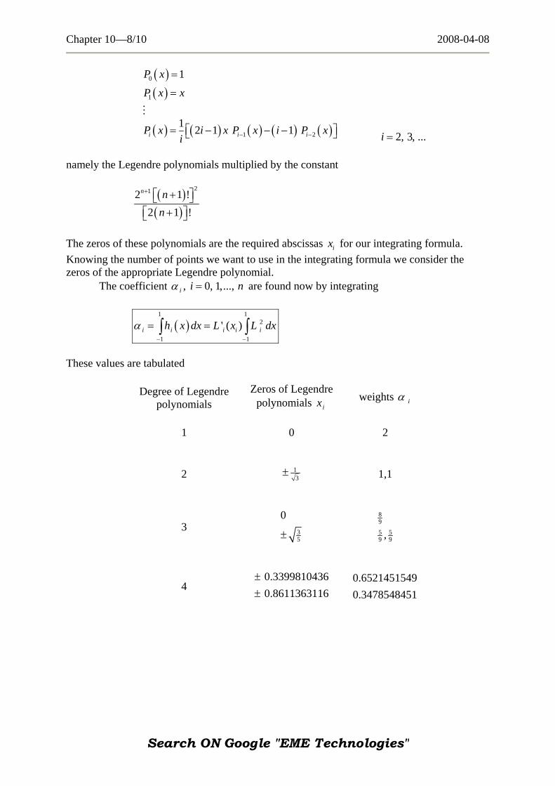
Chapter 10—8/10 2008-04-08

( )0 1P x =

( )1P x x= M

( ) ( ) ( ) ( ) ( )1 21 2 1 1i iP x i x P x i P xi − −= − − −⎡ ⎤⎣ ⎦i 2, 3, ...i =

namely the Legendre polynomials multiplied by the constant

( )( )

212 12 1 !

n nn

+ +⎡ ⎤⎣ ⎦+⎡ ⎤⎣ ⎦

!

The zeros of these polynomials are the required abscissas ix for our integrating formula. Knowing the number of points we want to use in the integrating formula we consider the zeros of the appropriate Legendre polynomial. The coefficient iα , are found now by integrating 0, 1,...,i = n

( )1 1

2

1 1

' ( )i i i i ih x dx L x L dxα− −

= =∫ ∫

These values are tabulated

Degree of Legendre polynomials

Zeros of Legendre polynomials ix weights iα

1

0

2

2

13

±

1,1

3

35

0

±

89

5 59 9,

4

0.33998104360.8611363116

±±

0.65214515490.3478548451


Chapter 10—9/10 2008-04-08

10.3.2. Composite Gaussian – Legendre integration

( )1 1

10 0 0

12 2 2

m m nj

i i ii i j

h yhI I f x xα− −

+= = =

i⎡ ⎤

= = + +⎢ ⎥⎣ ⎦

∑ ∑ ∑

where , iy 0, 1, ...,j n= are the zeros of the ( )1 thn + degree of Legendre polynomials.

10.3.3. Summary of the Gaussian integration

( )1

112 2 2 2 2

b n

iia

b a b a a b b a b a a bF z dz F x dx F xα=−

− − + − −⎛ ⎞ ⎛ ⎞= + =⎜ ⎟ ⎜ ⎟⎝ ⎠ ⎝ ⎠

∑∫ ∫ 2+

+

where iα and ix are taken from the table. This formula is exact for polynomials up to the

order. Usually the composite formula is being used. 2n −1

F(z)

za bzi zi+1

h

( )1 1

10 0 0

12 2 2

m m ni

i j ii i j

h zhI I F z zα− −

+= = =

i⎡ ⎤= = + +⎢ ⎥⎣ ⎦

∑ ∑∑

0 1 ... ma z z z b= < < < = 1i iz z+ h− = 0, 1, ..., 1i m= −

10.3.4. Special topics Numerical integration can not be directly applied in case of singularity or infinite intervals. The following measures may be applied then 1) The use of the weight functions and special quadratures

( ) ( ) ( ) ( )0

b b n

i iia a

if x dx w x x dx x Eγ α γ=

= = ∑∫ ∫ +

Such approach is useful in case of singularities, for selected types of singularity. As a result we come to Gauss – Chebyshev, Gauss – Laguerre, Gauss – Jacobi etc. formulas


Chapter 10—10/10 2008-04-08

2) General way of dealing with singularities

Example

1

0 1x dx

x−∫ - Approach: remove singularity by means of integration by parts

first and apply numerical integration then

1 11

00 0

2 1 2 1 2 11x dx x x x dx x dx

x= − ⋅ − + − = −

−∫ ∫1

0∫

2x

3) Integrals with infinite limits Approach: eliminate infinite limits by appropriate change of variable

Example

2 21

2 2 2

0 0 1

e e ex xx dx x dx x dx∞ ∞

− −= +∫ ∫ ∫ −

Let 2 1x y−= → 32

12

dx dyy

= −

1

2 2

52

1 12 2

1 20 0 0

1 ee e2

yx xx dx x dx dy I I

y

−∞− −= + =∫ ∫ ∫ +

Remarks

(i) integration by parts required

1 1

5 32 2

1 1

0 0

e 1 1 e2

y y

dy dy etcey y

− −

= + →∫ ∫

(ii) singularity due to 1ye

− remains

(iii) ( )1

1 1

3 3 122 2

11 1 1 1 122

20 0 0 0

e1 e 1 e 1 1 32 2 2 4 8

yy y

ydydy dy y e dy

eyy y y

−− −− −

−−= = = +∫ ∫ ∫ ∫

and

11

20

lim 0y

yy e

+

−

→=


numerical methods in civil engineering method.pdf · numerical differentiation and integration....

Documents