numerical methods in scientific computation - …jinbo/courses/numericalmethods_fall2011/jb... ·...

CSE 3802 / ECE 3431Numerical Methods in Scientific

Computation

Jinbo BiDepartment of Computer Science & Engineering

http://www.engr.uconn.edu/~jinbo

1

The Instructor• Ph.D in Mathematics• Previous professional experience:

– Siemens Medical Solutions Inc.– Department of Defense, Bioanalysis– Massachusetts General Hospital

• Research interests: biomedical informatics, machine learning, data mining, optimization, mathematical programming,

• Apply machine learning techniques in medical image analysis, patient health records analysis

• Resume is at http://www.engr.uconn.edu/~jinbo2

http://www.engr.uconn.edu/~jinbo/�

Numerical Methods, Fall 2011 Lecture 1 3

• Lectures are Tuesday and Thursday, 9:30 –10:45 am

• No specific lab time, but significantcomputer time expected.

• Computers are available in ITEB C25 and C27.

Class Meetings

Prof. Jinbo Bi CSE, UConn

4

• Homework will be assigned once every week or two and due usually the following week.

• You may collaborate on the homework, but your submissions should be your own work.

• Grading:• Homework 30%• Exam 1 and 2 40%• Final Exam 30%

Class Assignments

Numerical Methods, Fall 2011 Lecture 1


5

• MATH 2110Q Multivariate Calculus• Taylor series• MATH 2410Q Introduction to Differential

Equations • Integration• Linear Algebra

Mathematical Background



6

• Languages to be used:• Matlab, C, C++

• CSE 1100/1010 programming experience

• Any OS is acceptable

Computer Background



7

• Go over the course syllabus• Course websitehttp://www.engr.uconn.edu/~jinbo/Fall2011_

Numerical_Methods.htm

Syllabus



http://www.engr.uconn.edu/~jinbo/Fall2011_Numerical_Methods.htm�

http://www.engr.uconn.edu/~jinbo/Fall2011_Numerical_Methods.htm�

8

Today’s Class:• Introduction to numerical methods• Basic content of course and class

expectations• Mathematical modeling



9

Introduction• What are numerical methods?

• “… techniques by which mathematical problems are formulated so that they can be solved with arithmetic operations.” (Chopra and Canale)

• What type of mathematical problems?• Roots, Integration, Optimization, Curve

Fitting, Differential Equations, and Linear Systems



Introduction• How do you solve these difficult

mathematical problems?• Example: What are the roots of x2-

7x+12?• Three general non-computer methods

• Analytical• Graphical• Manual

10Numerical Methods, Fall 2011 Lecture 1


• This is what you learned in math class• Gives exact solutions• Example:

• Roots at 3 and 4• Not always possible for all problems and

usually restricted to simple problems with few variables or axes

• The real world is more complex than the simple problems in math class

Analytical Solutions

)4)(3(1272 −−=+− xxxx



Graphical Solution



• Using pen and paper, slide rules, etc. to solve an engineering problem

• Very time consuming• Error-prone

Manual Solution



Numerical Methods• What are numerical methods?

• “… techniques by which mathematical problems are formulated so that they can be solved with arithmetic operations.” (Chopra and Canale)

• Arithmetic operations map into computer arithmetic instructions

• Numerical methods allow us to formulate mathematical problems so they can be solved numerically (e.g., by computer)



• What is this course about?• Using numerical methods to solve

mathematical problems that arise in engineering

• Most of the focus will be on engineering problems

Course Overview



• Introduction• Programming• Mathematical Modeling• Error Analysis

• Mathematical Problems• Roots, Integration, Optimization, Curve

Fitting, Differential Equations, and Linear Systems

Basic Materials



A mathematical model is the formulation of a physical or engineering system in mathematical terms.

• Empirical• Theoretical

Mathematical Modeling



• Dependent variable = f ( independent variables, parameters, forcing functions )

• In an electrical circuit, I = V/R; The current, I, is dependent on resistance parameter, R, and forcing voltage function, V.

Mathematical Modeling



• What is the velocity of a falling object?• First step is to model the system• Newton’s second law

• Total force is gravity and air resistance

Example 1

mF

dtdv

mFamaF =⇒=⇒=

cvmgFFF AirGravity −=+=



• First order differential equation• Analytical solution

Example 1

vmcg

mcvmg

mF

dtdv

−=−

==

)1()( tmc

ec

gmtv −=



• m=68.1kg, c=12.5 kg/s

Example 1



• What if we can’t find an analytical solution?

• How do you get a computer to solve the differential equation?

• Use numerical methods

Example 1



• Use the finite divided difference approximation of the derivative

• The approximation becomes exact as Δt → 0

Euler’s Method

ii

ii

tttvtv

dtdv

−−

=+

+

1

1 )()(



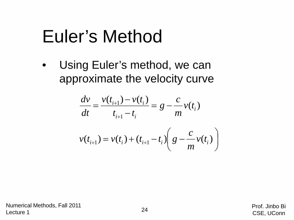
• Using Euler’s method, we can approximate the velocity curve

Euler’s Method

)()()(

1

1i

ii

ii tvmcg

tttvtv

dtdv

−=−−

=+

+

−−+= ++ )()()()( 11 iiiii tv

mcgtttvtv



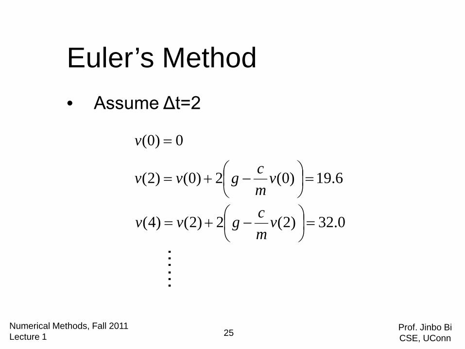
• Assume Δt=2

Euler’s Method

0)0( =v

6.19)0(2)0()2( =

−+= v

mcgvv

0.32)2(2)2()4( =

−+= v

mcgvv

……



Euler’s method



• Avoids solving differential equation• Not an exact approximation of the

function• Gets more exact as Δt→0• How do we choose Δt? Dependent on

the tolerance of error.• How do we estimate the error?

Euler’s Method



Example 2• Find i(t)

resistor

capacitorVolt supply

switch



Example 2

• Analytical solution

)()( tvtRiV c+=

dtdvCti c=)(

))((1 tvVRCdt

dvc

c −=

−= RC

t

c eVtv 1)(

RCt

c eRV

dtdvCti

−==)(



Example 2• Numerical solution

)()( tvtRiV c+=

dtdv

dtdiR c+=0

Cti

dtdiR )(0 +=

)(1 tiRCdt

di−=



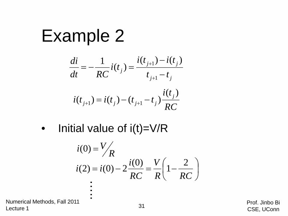
Example 2

• Initial value of i(t)=V/R

jj

jjj tt

tititi

RCdtdi

−−

=−=+

+

1

1 )()()(1

RCti

tttiti jjjjj

)()()()( 11 −−= ++

RVi =)0(

−=−=

RCRV

RCiii 21)0(2)0()2(

…..



Next class• Programming and Software• Read Chapters 1 & 2



numerical methods in scientific computation - …jinbo/courses/numericalmethods_fall2011/jb... ·...

Documents