numerical methods of nonlinear optimal control based on mathematical programming

Pergamon Nonlinear Analysis, Theory, Methods & Applications, Vol. 30, No. 6, pp. 3843-3854, 1997

Proc. 2nd World Congress ofNonlinear Anu!,sts 0 1997 Elsevier Science Ltd

Printed in Great Britain. All rights reserved

PII: SO362-546X(%)00327-6 0362-546X/97 S 17.00 + 0.00

NUMERICAL METHODS OF YONLINEAR OPTIMAL CONTROL BASED ON MATHEMATICAL PROGRAMMING

SATOSHI IT0

The Institute of Statistical Mathematics: Department of Prediction and Control

4-6-7 Minami-Azabu, Minato-ku, Tokyo 106, Japan

Key words and phrases: Optimal control, interior point method, convex quadratic programming, inexact Newton method, quasi-Newton method, sequential quadratic programming, nonlinear programming,

infinite programming.

1. INTRODUCTION

Some approaches to the numerical solution of discrete-time optimal control problems have been proposed by using interior point algorithms within the framework of sequential quadratic programming. (See, e.g., Wright [32] and Leibfritz and Sachs [13].) Those problems are discretized versions of continuous-time optimal control problems and hence potentially very large. Interior point algorithms are iterative methods, and at each iterate one has to solve simultaneous systems of linear equations. Most computational time is spent in solving the systems of linear equations. Therefore it is a crucial key to practical implementation to solve them in a most efficient manner. For large-scale problems it is also essential to exploit the sparsity of coefficient matrices.

In the first half of this paper, we study a primal-dual interior-point algorithm for convex quadratic programming problems in Hilbert space with the object of direct application to continuous-time LQ optimal control problems. See Megiddo [IS], Tanabe [26. 271, Kojima et al. [ll] and Monteiro and Adler [17] for original primal-dual interior-point algorithms in finite-dimensional spaces. Ito et al. [8] first proposed a primal-dual interior-point algorithm for linear programming in the infinite- dimensional setting. Since our problems are infinite-dimensional, it is impossible in general to solve exactly the linear equations for finding a search direction at each iterate. We consider an inexact implementation of the algorithm based on the analysis in [8].

On the other hand, quasi-Newton methods have been generalized to Hilbert space mainly with the object of applying to optimal control problems [5, 12: 19, 28, 29, 2) 30, 31, 15. 3, 21, lo]. A family of quasi-Newton methods is now recognized as one of the most efficient algorithms for unconstrained optimal control problems. However, there is no efficient and general-purpose algorithm for constrained optimal control problems. Some algorithms are effective for certain classes of problems. For problems with bounded control variables, modified CG methods were studied by Pagurek-Woodside [18] and Quintana-Davison [20], and a modified quasi-Newton method by Edge-Powers [2]. Jacobson et al. [9] proposed a transformation technique by means of slack variables for problems with state-variable inequality constraints. Shimizu et al. [22] d eveloped a feasible direction method and a quasi-Newton method for problems with a finite number of inequality constraints.

We study in the latter half of the paper a dual sequential quadratic programming framework for a general class of constrained optimization problems in Hilbert space. In this framework, quadratic programming subproblems, with the Hessian of the Lagrangean replaced by its approximation, are iteratively solved to generate a sequence of search directions. This paper includes two applications of the dual SQP method-one is an application to optimal control problems with terminal-state equality constraints [6], and the other is an application to the so-called state-constrained optimal

3843

3844 Second World Congress of Nonlinear Analysts

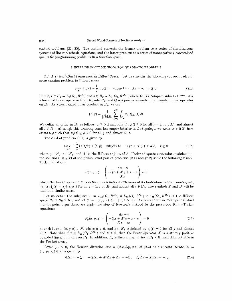
control problems [23, 251. The method converts the former problem to a series of simultaneous

systems of linear algebraic equations, and the latter problem to a series of nonnegatively constrained

quadratic programming problems in a function space.

2. INTERIOR POINT METHODS FOR QUADRdiTIC PROBLEMS

2.1. A Primal-Dual Frameworlc in Hilbert Space. Let us consider the following convex quadratic

programming problem in Hilbert space:

min (c, Z) + 5 (z. Qz) subject to Ax = b. x 2 0. % (2.1)

Here c. x E HI = Lz(Qr, R”1) and b E H2 = Lz(&, R”?), where 0% is a compact subset of RI’;. A is

a bounded linear operator from HI into Ha. and Q is a positive-semidefinite bounded linear operator

on HI. As a normalized inner product in Hi. we use

(x3 Y) = ,Qi;Mi j=l . R, xj(t)yj(t) & cl We define an order in H1 as follows: 5 > 0 if and only if zj(t) > 0 for all j = 1: . , Ml and almost

all t E fir. Although this ordering cone has empty interior in &-topology: we write z > 0 if there

exists a p such that xj(t) 2 p > 0 for all j and almost all t.

The dual of problem (2.1) is given by

max - f (x,&x) + (b, y) subject to -Qx+A”y+z=c. 210. (2.2) z.y,z

where y E Hz% z E HI: and A” is the Hilbert adjoint of A. Under adequate constraint qualification,

the solutions (x. y, Z) of the primal-dual pair of problems (2.1) and (2.2) solve the following Kuhn

Tucker equations:

Ax - b F(x, y, z) =

(

-Qx+A*y+z-c =O. XZ 1

where the linear operator X is defined, as a natural extension of its finite-dimensional counterpart,

by (Xz)] (t) = xj(t)zj(t) for all j = 1, , Ml and almost all t E 01. The symbols 2 and D will be

used in a similar sense.

Let us define the subspace L = L,( &?I, R”*l) x L,(Rz: R.“z) x L,(&. RM1) of the Hilbert

space H1 x Hz x HI. and let F = { (z,~,z) E L ] Z, z > 0 }. As is standard in most primal-dual

interior-point algorithms, we apply one step of Newton’s method to the perturbed KuhnTucker

equations:

Ax-b Fp (x. y. z) = -Qx+A’y+z-c

Xz-pe (2.3)

at each iterate (x, y> Z) E F, where p > 0, and e E H1 is defined by eJ(t) = 1 for all j and almost

all t. Note that if 5 E L,(~‘I, R”‘) and x > 0, then the linear operator X is a strictly positive

bounded linear operator on HI. In addition. Fp is then a map to Hz x H1 x HI and differentiable in

the Frechet sense.

Given pLc > 0. the Newton direction Aw = (Ax,Ay,Az) of (2.3) at a current iterate w, =

(2,. y,, z,) E F is given by

AAx = -&., -QAx + A*Ay + AZ = --cc, .&Ax + X,Az = -rc, (2.4)

Second World Congress of Nonlinear Analysts 3845

where

& = Ax, - b) Cc = -&xc + A*y, + .zc - c, T , = Xcz, - p,e (2.5)

denote the corresponding residuals of (2.3) at w,. Whenever x,.z E 1;,(01, R”l) and 2,~ > 0, we can define a strictly positive bounded linear operator D on HI by D2 = XZ-l. Under some practically mild assumptions, the operator A(Q + D-2)-‘A* is invertible on Loo(&, R”2) for any d E L,( 01, R”“), d > 0, and the Newton direction Aw = (Ax, Ay, AZ) is given as follows:

Ay = (A(Q + D,‘)-‘A*)-1 (--EC - A(Q + D,2)-1(& - X,'T,)),

Ax = (Q + DF2)-l(A*Ay + CC: - X,‘rC), (2.6) AZ = -DF2Az - XC-%-,.

Finally, we must specify how to choose pLc and a stepsize in the Aw direction. We use the following rules for the choice of pLc and the computation of the next. iterate w+ = (x+, y+, z+):

pL, = oc(x,, z,) fclr some oC E (0. l), (2.7)

--7c min(X,‘Ax, Ziml AZ) >

for some rC E (0, l), (2.8)

w+ = w, + ol,Aw. (2.9)

Each iterate of the algorithm consists of (2.7), (‘L!.5), (2.6), (2.8) and (2.9) for some initial iterate wg = (x0, YO, zo) f .F.

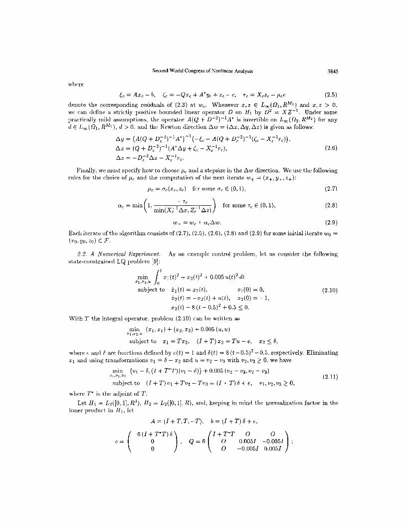
2.2. A Numerical Experiment. As an example control problem, let us consider the following stat,e-constrained LQ problem [9]:

.I

1

min xl@)2 + x2( t)2 + 0.005 u(t)2 dt ~l,Z?,U 0 subject to c&(t) = x2(t), q(O) = 0.

c&J(t) = -.x2(t) + u(t), 40) = -1,

x2(t) - 8 (t - 0.5)2 + 0.5 5 0.

With T the integral operator. problem (2.10) can be written as

(2.10)

min (21. Xl) + (x2: x2) .t 0.005 (u, u) ~1JZ.U subject to x1 = Tx2, (I + T) 22 = Tu - e, 22 5 6,

where e and 6 are functions defined by e(t) = 1 and 6(t) = 8 (t - 0.5)2 - 0.5, respectively. Eliminating x1 and using transformations 01 = S - x2 and u = 712 - V:S with 212,1)3 >_ O> we have

u;n& (VI - 4 (I+ T*T)( 211 - ii)) + 0.005 (?I:! - v3,v2 - v3)

subject to (I + T) ~1 + Tv2 -. Tv3 = (I + T) 6 + e, (2.11)

~1,712, v3 2 0,

where T” is the adjoint. of T.

Let HI = ~52([0,1], R3), H2 = ~52([0,11, R), and, keeping in mind the normalization factor in the inner product in HI, let

A= (I+T,T.-T), b= (I+T)h+e,

c= ( -6(I;T*T’o),


then problem (2.11) corresponds to the primal form (2.1).

The primal--dual interior-point algorithm was applied with setting gk = 10P2 and rk = 0.99. As an initial estimate, (20, yo, 20) = (( e, e, e), 0) e) was chosen, which is infeasible for both the primal and dual. We must solve two kinds of linear equations to find the dual search direction Ay. A pre- conditioned CG method was used for the imrer linear equation and was terminated when the relative residual was less than 10e5. For the outer linear equation. a CG method (without preconditioning) was terminat,ed when t,he relative residual was less than lo- 2. All functions were discretized at a finite number of points, and all integrals in the definitions of inner products and integral operators were approximated with the trapezoidal rule. Table 1 shows the result for 201 points. The CG column shows the number of CG iterations required for solving the outer linear equation. Taking account of the constant term (S, (I+T*T) 6) NN 3.938 x 10-l, which was omitted during the problem formulat,ion, we can see that the objective value of problem (2.10) is 1.700 x 10-l after 12 iterations.

Table 1

! i 7r = (Sk,%.) YkIYk-1 primal obj. Kkll IIC~II CG ak 0 1.000e+00 1 5.658~01 2 5.1546-01 3 4.2298-01 4 2.824~01 5 1.659~01 6 8.788~02 7 4.432~02 8 1.672~02 9 4.854e-03

10 1.207~03 11 3.035.c04 12 7.485~05 13 1.182~05 14 2.561e-06 15 3.341e-07

5.658~01 9.109e-01 8.205~01 6.678~01 5.875~01 5 296e-01 5.043e-01 3.773e-01 2.903e-01 2.487~01 2.514~01 2.466~01 1.579e-01 2.166~01 1.305e01

9.332.e01 2.594e-01 1.751e-01 3.805~02

-1.195.Y01 -1.946e-01 -2.160~01 -2.245~01 -2.256~01 -2.245~01 -2.240~01 -2.239e-01 -2.238s~01 -2.238e-01 -2.238~01 -2.238~01

7.221~~01 4.344.P01 3.960e-01 3.263~01 2.233~01 1.380e-01 7.758e02 3.951e-02 1.475~02 4.035e-03 9.028a-04 2.052~04 4.911e-05 9.855e-06 3.218~06 1.245~06

4.122e+OO 2.485e+OO 2.265e+OO 1.866e+oo 1.273e+OO 7.896e-01 4.438~01 2.279e-01 8.493e-02 2.318~02 5.291e-03 1.238~~03 2.866~04 4.129e-05 8.552~06 1.077~06

3 3.973e-01 5 8.849.Y02 3 1.762e-01 3 3.177e-01 5 3.797e-01 5 4.380~01

13 4.865~01 12 6.273~01 18 7.271~01 34 7.718~01 63 7.661~01 80 7.688~01 85 8.567e-01

204 7.951e-01 262 8.805e-01

2.3. Inexact Implementation. The search direction Aw = (As, Ay, AZ) at each iterate is given by (2.6). However, since this include linear equations in L2! it is impossible to solve it exactly using direct solvers. So, as we did in the preceding section, we try to solve it approximately by an iterative scheme which terminates when the relative residual is sufficiently small. It is worth studying the inexact implementation of the primalldual interior-point algorithm in this sense.

For simplicity, let us assume the situation where we can exactly (or almost exactly) solve the inner linear equation in (2.6), which is common because Q has a simple structure for most control problems. When we approximately solve the outer linear equation in (2.6), the resulting direction Aw = (Ax, Ay, Az) is given by

ay = (A@ +o;~)-~A*)-~(-~~ - A(Q+D;~)-~(C~ -x;~~~) +T& Ax = (Q + DF2)-‘(A*Ay + Cc - X;‘rJ, (2.12)

2 1 AZ = -DC- Ax - X, rc,

where 71~ denotes the residual for the outer linear equation. Then Aw satisfies

AAx = -& + vc, -&Ax + A*Ay + AZ = -SC, &Ax + X,A.z = -rc. (2.13)

Namely, the inexact solution of the outer linear equation only affects the primal feasibility condition. Hence if we choose a dual-feasible solution as an initial iterate, then all the iterates remain dual- feasible even under the inexact iteration. See Ito et al. [8] for the details of its local convergence property.


3. DUAL SEQUENTIAL QUADRATIC PROGRAMMING FOR GENERAL NONLINEAR PROBLEMS

Let us next consider the following constrained optimization problem:

min f(u) subject to G(u) E C, u (3.1)

where U and Y are real Hilbert spaces, C is a nonempty closed convex cone in Y, f : U --+ R and G : U + Y are twice continuously Frechet differentiable.

Define the Lagrangean functional L : U x Y -+ R as

L(u, A) g j(u) + (G(u), A).

The Kuhn-Tucker type optimality condition for problem (3.1) is given as follows.

THEOREM 3.1 (GENERALIZED KUHN-TUCKER, THEOREM) [14. 11. Suppose that u E U is a regular point of the constraint G(u) E C. If u is an optimal solution of problem (3.1), then there exists a X E Y such that

V,L(u, X) = of(u) + VG(u)X = 0, (3.2a)

G(U) E C, (G(u),X) = 0, X E C*, (3.2b)

where C’ denotes the polar cone, Vf(u) the gradient of f at u, and VG(u) the Hilbert adjoint of G’(U).

REMARK 3.1. The regularity assumption in this paper, means that some constraint qualification should be satisfied. For example, a point u is said to be regular in the sense of the Kuhn--Tucker constraint qualification if the subset { ((G(u). y), VG(u)y) E R x U : y E C* } is closed and if for any s E U satisfying G(u) + G’(u)s E C there exists a map E : [0, 1) -+ U such that (i) E(0) = u, that (ii) G(E(t)) E C for all t E [0, l), and that (iii) FL$ (E(t) - E(O))/t = s.

We shall apply Newton’s method to the optimality condition (3.2). Linear approximation to (3.2) at a point (&, X”) leads to the following update formula:

of@) + V2,,L(u”, X’“)(u”” - z?) + VG(u”)X’+’ = 0. (3.3a) G(u”) + G’(uk)iu k+l -uk) E c: (3.3b)

(G(u’) + G’(uk)(uk+l - u’“), A”) + (G(u”), A”+ - A”) = 0, (3.3c)

xk+’ E C”, (3.3d)

where Vz,L denotes the Hessian of L with respect to u. Assuming that the variation of X is sufficiently

small, set .sk g u’+l - uk and pk g Xkfl (z X”). Then we have

Vf(u”) + VE,L(uk, r,‘“)sk + VG(u”)p’ = 0, (3.4a)

G(uk) + G’(u”)s’ E C: (3.4b)

(G(u”) + G’(uk).sk, p”) = 0, (3.4c)

pk I, CT*. (3.4d)

Suppose that sk is a regular point of the affine constraint G(u”) + G’(u”)s E C: then Theorem 3.1 shows that (3.4) is a necessary condition for sk to solve the quadratic programming problem:

mjn (s. Vf(uk)) + i(s. V2,,L(uk: X”)s) subject t,o G(u’“) + G’(uk)s E C. (3.5)

Condition (3.4) is also sufficient if V&,L(u’, Xk) is positive semidefinite. Then we may seek the solution .sk of problem (3.5) and the corresponding Lagrange multiplier pk instead of (uk+l, A”+‘) satisfying (3.3). This met,hod, however, has some demerits: the Hessian Vz,L(u”, X”) is not generally


easy to evaluate and is not necessarily positive semidefinite. So, with the Hessian replaced by a strictly positive, self-adjoint linear operator Bk, we consider the modified direction-finding problem:

rnjn (s, V~(U”)) + i(s, B”s) subject to G(u”) + G’(uk)s E C. (3.6)

The operator Bk is: of course, required to be in some sense an approximation to the Hes- sian VE,L(U’“, X”) and to be easy to evaluate.

An effective procedure for solving the direction-finding problem (3.6) would be to solve its dual problem. This procedure is particularly attractive when Y is finite-dimensional (i.e., the functional- constrained case) or when C = (0) (i.e., the equality-constrained case). Defining the dual functional u : Y -+ R as

v(p) 2 rnp (s, Vf(u”)) + f(s, Bks) + (G(d) + G’(u”)s,p),

we obtain a dual problem in the form

max U(P) subject to p E C*. P

(3.7)

(3.8)

The minimization in (3.7) is unconstrained and is attained by s = -(B&)-l (Vf(u.“) + VG(uk)p). The dual functional 21 and its gradient are then given by

v(p) = (G(u”)+) - ;((B’)-‘(Vf(u”) + VG(U~)&V~(U~) + VG(u”)p), (3.9)

VW(P) = G(u”) - G’(u’)(B”)-‘(Vf(u”) + VG(u’)& (3.10)

Problems (3.6) and (3.8) are related through the following duality theorem.

THEOREM 3.2. i) Suppose that sk E U is a regular point of the constraint G(u”) + G’(u’)s E C. If sic solves problem (3.6), then there exists a solution ,!L” E Y to problem (3.8) and it holds that

(sk, V~(U’)) + ;(s’. Bksk) = v(/L”).

ii) I f pk E Y is a solution to problem (3.8), then

Sk = -(B”)-1 (Vf(& + VG(u”)&

solves problem (3.6). and relation (3.11) holds.

(3.11)

(3.12)

REMARK 3.2. Duality holds under any constraint qualification. In fact, the regularity of .sk is only used to ensure the existence of the Lagrange multiplier for the primal constraint. Note that the Lagrange type duality theorem usually assumes Slater’s qualification (see, e.g., [14]). Both problems (3.6) and (3.8) are quadratic programming problems in Hilbcrt space, but the latter is easier to solve than the former since t.he constraint, is much simpler. Note that. if C = {0}, problem (3.8) has no constraint,s: if Y is finit,e-dimensional, problem (3.8) is finite-dimensional.

The modified Newton method wit.h the dual subprocedure above can be considered a generalization of t,he dual sequential quadratic programming (SQP) algorith m suggested by Han [4] to Hilbert space if t,he quasi-Newt,on updates arc used to generat,e Bk. It, is desirable in the dual SQP algorithm to know t,he representation of the inverse (B”)-’ rather than B” itself. The BFGS formula, a typical quasi-Newt,on update rule, is given as follows:

IP”>P’“[ lp? (B”)-‘q”[ _ ](Bk)-‘q”,p’“[, -- (P”? (Ik) (P,“, qk) cPk > qk)

(3,13)

where p k g Uk+l _ Uk qk & v,L(uk+l ,I,,~) - V,L&‘“, p’) ( and ] , . [ denotes a dyadic operator

defined on U by ]u’, u’[ d k (u’, d)u’ for each d E U. This formula is usually used under slight


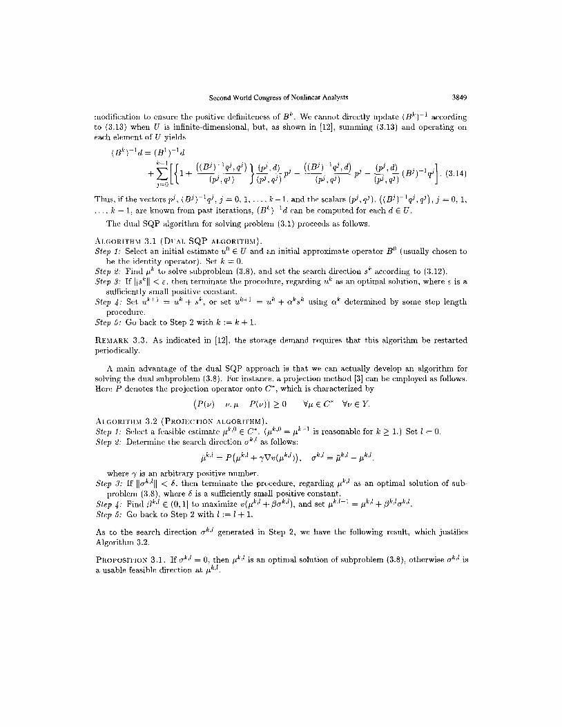
modification to ensure the positive definiteness of B’“. We cannot directly update (@)-I according to (3.13) when U is infinite-dimensional. but, as shown in [12], summing (3.13) and operating on each element of U yields

(B”)-‘d = (B’)-ld

Thus, if the vectors y’. (Bj)-lqj. j = 0. 1, . , .k- 1, and the scalars (p’, qj), ((Bj)-‘qj, qj), j = 0, 1, . k - 1, are known from past iterations. (Bk)-‘d can be computed for each d E U.

The dual SQP algorithm for solving problem (3.1) proceeds as follows.

-~LGORITHSI 3.1 (DVAL SQP ALGORITHM). Step 1: Select, an initial estimate u” E U and an initial approximate operator B” (usually chosen to

be the identity operator). Set k = 0. Step 2: Find CL’ to solve subproblem (3.8), and set the search direction .sk according to (3.12). Step 3: If l\skll < E, then terminate the procedure, regarding uk as an optimal solut,ion, where E is a

sufficiently small positive constant. Step 4: Set uk+l = uk + sk, or set uk+l = uL + aksk using crk determined by some step length

procedure. Step 5: Go back to Step 2 with k := k + 1.

REMARK 3.3. As indicated in [12]. the storage demand requires that this algorithm be restarted periodically.

A main advantage of the dual SQP approach is that we can actually develop an algorithm for solving the dual subproblem (3.8). F or instance. a projection method [3] can be employed as follows. Here P denotes the projection operator onto C”, which is characterized by

(P(v) - V./i - P(v)) 2 0 VP E c* vv E Y.

ALGORITHM 3.2 (PROJECTION ALGORITHM). Step 1: Select a feasible estimate pk,’ E C”. (,11’,’ = /.?-l 1s reasonable for k 2 1.) Set 1 = 0. Step 2: Determine the search direction gk.’ as follows:

P -IcJ = P(/&’ + yr7v($9), ,k,l = pk,l - #J,

where y is an arbitrary positive number. Step 3: I f Ilgk.‘ll < 6, th en terminate the procedure, regarding pk,’ as an optimal solution of sub-

problem (3.8), where 6 is a sufficiently small positive constant. Step 4: Find p’,’ E (0, l] to maximize ZI($.’ t- @a”$, and set $,‘+l = pk,’ + pk.‘ak,‘. Step 5: Go back to Step 2 with 1 := 1+ 1.

As to the search direction gk,’ generated in Step 2, we have the following result, which justifies Algorithm 3.2.

PROPOSITION 3.1. If ok.’ = 0, then ,uk,l is an optimal solution of subproblem (3.8), otherwise ok,’ is a usable feasible direction at pk”.


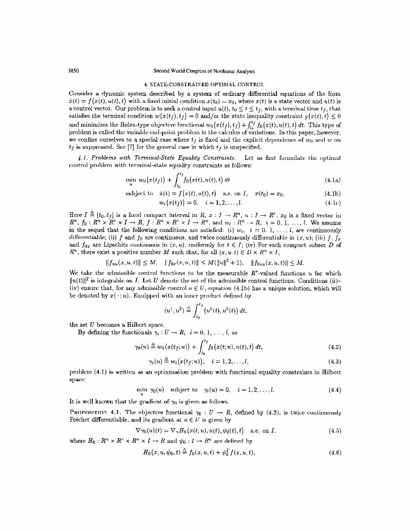
4. STATECONSTRAINED OPTIMAL CONTROL

Consider a dynamic system described by a system of ordinary differential equations of the form k(t) = f(~(t),~(t),t) with a fixed initial condition z(to) = ~0, where z(t) is a state vector and u(t) is a control vector. Our problem is to seek a control input u(t), to 2 t 5 tf, with a terminal time tf, that satisfies the terminal condition zu (z(tf), tf) = 0 and/or the state inequality constraint g(z(t)>t) 5 0

and minimizes the Bolza-type objective functional wo(z(tf),tf) +st”, fo(z(t),~(t), t) dt. This type of problem is called the variable end-point problem in the calculus of variations. In this paper, however, we confine ourselves to a special case where tf is fixed and the explicit dependence of 2~0 and zu on tf is suppressed. See [7] for the general case in which tf is unspecified.

4.1. Problems with Terminal-State Equality Constraints. Let us first formulate the optimal control problem with terminal-state equality constraints as follows:

m,‘” wo(x(tf)) + J

tf fo(4tbW) dt (4.la)

subject to i(t) =*)(z(t),~(l),l) a.e. on I, x(to) = 203 (4.lb)

wi(x(tf)) =O, i=1,2 ,..., 1. (4.lc)

Here 1 L [to, t,] is a fixed compact interval in R, x : I + R”, u : I + R’, x0 is a fixed vector in R”, f. : R” x R’ x I + R, f : R” x R’ x I -+ R”, and wi : R” -+ R! i = 0, 1, . , 1. We assume in the sequel that the following conditions are satisfied: (i) wi, i = 0, 1, . , 1, are continuously differentiable; (ii) f and fo are continuous, and twice continuously differentiable in (z, u); (iii) f? fz and fez are Lipschitz continuous in (x,~), uniformly for t E 1; (iv) For each compact subset D of Rn, there exist a positive number M such that, for all (x,u,t) E D x Rn x I,

Ilfuu(~,u~~)ll 5 M, IlfOz(~,U,~)II I wl1412 + I), IlfOuu(~,~,~)ll 5 hf. We take the admissible control functions to be the measurable R’-valued functions u for which llu(t)l12 is integrable on I. Let U denote the set of the admissible control functions. Conditions (ii)- (iv) ensure that, for any admissible control u E U, equation (4.lb) has a unique solution, which will be denoted by x(. ; u). Equipped with an inner product defined by

(u’:u2) g 1;’ (u’(t),u2(t)) dt,

the set U becomes a Hilbert space. By defining the functionals yi : U + R, i = 0, 1, . . . , 1, as

TO(U) k wo(x(tp)) + ~~~lio(5(t;~~,~(t).t) dt, (4.2)

-yi(u) g wi(s(tf; u)), i = 1,2,. . . ,I, (4.3)

problem (4.1) is written as an optimization problem with functional equality constraints in Hilbert space:

min 70(u) subject to n(u) = 0, i = 1,2,. . ,l. 21 (4.4)

It is well known that the gradient of yo is given as follows.

PROPOSITION 4.1. The objective functional yo : U + R, defined by (4.2), is twice continuously Fr6chet differentiable, and its gradient at u E U is given by

Vyo(u)(t) = V,Ho(x(t;u),u(t),~~(t),t) a.e. on I, (4.5)

where Ho : Rn x R’ x R” x I -+ R and $0 : I + Rn are defined by

Ho(a:,u,$o,t) k fo( x,u,t) +Gf(v,t), (4.6)

Second World Congress of Nonlinear Analysts 385 1

40(t) = -‘C7,Ho(z(t;u),u(t),~o(t),t), tio(tj) = Vwo(“(tf;“)), (4.7)

respectively.

The gradients of y;, i = 1, 2, . . . . I, are given i.n the same manner.

PROPOSITION 4.2. The constraint functionals yz : U -+ R, i = 1, 2, . , 1, defined by (4.3), are twice continuously Frkchet. differentiable, and t!heir gradients at u E U are given by

V-f,(u)(t) = V,Hi (z(t; u), u(t), $j(t), t) a.e. on I, (4.8)

where, for each i, H, : R” x R’ x R” x I + R and $i : I + R” are defined by

Hi(z>u,W) 2 @f(z,u,t), (4.9)

&(t) = -V,Hi (z(t: u)> u(t)> h(t). t) % $i,i(tr) = VW (z(tr; u)), (4.10)

respectively.

The following lemma gives a regularity condition.

LEMMA 4.1. Let an admissible control u E U s,atisfy the following two conditions: i) (Local control- lability) For any e E R” there exist,s an s E U such that

i(t) = f~(~c(t;u),21(t):t)l(t) + fu(z(t;~),~(t),t)s(t) a.e. OII I, [(to) = 0. and [(tf) = e;

ii) Vw;(z(tf; u)), i = 1, 2, . . . , I, are linearly independent in R”. Then the gradients Vyi(u): i = 1, 2, . , I. are linearly independent in U, that is. u is a regular point of the functional constraints n(u) = 0,

i = 1, 2, . . . , 1.

The quasi-Newton direction-finding problem for problem (4.4) is given as follows:

min (.s. Vyo(u”)) + i(.s- B”s) subject to s

Ye + (s,Vy,(u”)) = 0. i = 1,2.. ,l, (4.11)

whose dual is given by

(4.12)

@f g yj(u”) - (Vyi(u’), (B”)-lVyo(~k)), i = 1,2,. . : 1,

A$ g (Vyj(,u’“), (El’;)-‘Vyj(d)), i,j = 1,2,. . ,l.

Theorem 3.2 is restated for problems (4.11) and (4.12) as follows. Note that the regularity of sk is unnecessary since the constraint in (4.11) consists of a finite number of Seine functionals.

COROLLARY 4.1. i) I f sk E U solves problem (4.11), th en there exists a solution pk E R’ to problem (4.12). ii) For a solution p” E R’ of problem (4.12): set

Sk = -(B”)-‘Vyo(uk) - ~p~(Bk)--lvyj(uk); (4.13) i=l

then sk solves problem (4.11) and pk is the corresponding Lagrange multiplier.

It immediately follows from the strict positivity of B” that A” is positive semidefinite (but not necessarily positive definite). Since a necessary and sufficient condition for problem (4.12) is that

ilk/L = p”, (4.14)


we only need to solve this simultaneous system of linear equations and set sk according to (4.13). Note that the positive definiteness of A” corresponds to the linear independence of Vyi(u”), i = 1, 2,

. ~ 1.

4.2. Problems with State Inequality Constraints. Let us next consider the following optimal control problem with state-variable inequality constraints over the fixed compact interval I:

I

t f Ti,n wo(x(tf)) + fo(x(WW) dt (4.15a)

subject to k(t) =‘Pf(r(t),~(t),t) a.e. on I, xc(to) = x0, (4.15b)

g(x(t),t) IO on I, (4.15c)

where x : I -+ R”, u : I --f R’, x0 E Rn; wo : R” -+ R, f. : R” x R’ x I + R, f : R” x R’ x I --+ R”, and g : R” x I + R”. In addition to conditions (i)-(iv) in Section 4.1, we assume that (v) g is continuous, and continuously differentiable in x. We take the class of admissible controls to be L2(1, R’), the set of all square-integrable functions from I into R’. Conditions (ii)- ensure that, for any admissible control U, equation (4.15b) h as a unique continuous solution, which will be denoted by z(.;u).

Let U g &(I, R’) and Y e &(I, R”). The spaces U and Y are Hilbert when equipped with the inner products defined by

(u1,u2) 2 tot’ (u1(t),u2(t)) dt, J (y1,y2) A ~otf(y1(t)~y2(t)) dt.

respectively. Let Y- (resp., Y+) denote the negative (resp., positive) cone in Y consisting of functions nonpositive (resp., nonnegative) almost everywhere on I. Note that Y- and Y+ are nonempty closed convex cones in Y and that Y+ = (Y-)*. Further, let us define the functional 7s : ZJ + R and the operator G : U + Y as follows:

-ro(u) g wo(x(tf; u,) + J

if

fo(z(t:uMt)>t) dt, (4.16)

G(u)(t) k g(x(i;u), t) on I. (4.17)

Problem (4.15) is now reformulated as an optimization problem in Hilbert space:

rnjn ye(u) subject to G(U) E Y- (i.e., G(U) 2 0). (4.18)

The gradient of 70 is given by Proposition 4.1. It is necessary to know the representation of the derivative of G in order to apply the dual S&P algorithm to problem (4.18). The following theorem concerns the differentiability of G.

THEOREM 4.1. The constraint operator G : U -+ Y, defined by (4.17), is twice continuously Frechet differentiable. The derivative G’(U) E L(U, Y) of G at u E U is given by

(G’W) (t) = .h’fL (47; u), 471, P(t, T), .)44 d7 a.e. on I Vs E U, (4.19)

and its adjoint VG(u) E L(Y, U) is given by

(VG(u)p)(t) = ~“V,,Hjz(t;.).,,(t),*(7:t),t)~(~)dr a.e. on I Vp E Y, (4.20)

where H : R” x R’ x RnXm xI+R”and9:T+Rnxm (T is a trapezoidal region { (t, T) E R2 : to 5 T 5 t 5 tf }) are defined by

H(x,u, 9, t) 2 !FTj(x, u, t), (4.21)

Second World Congress of Nonlinear Analysts

gP(t\r) = -V,H(~(T;u),u(T),~(t?T),T), !i?(i: t) = V,g(z(t; u). t).

respectively.

3853

(4.22)

Problem (4.15) can be solved by applying the dual SQP algorithm to problem (4.18). At each it,eration, the dual functional v, originally given by (3.9), is evaluated as follows: Calculate Vys(r?) according to (4.5); given an element p of Y, calculat,e VG(uL)p according to (5.6) and (B’;)-‘(Vys(‘cl”) + VG(&)p) according to (3.14): and set

4~) = t:‘(g(T(f:Irb).t).lL(t)) dt /

1 -- 2

J”( (P”)-’ (%o(& + W&P))(~), V~ob”)(t) + (WU”)P) NJ) dt. (4.23) to

In order to evaluat,e the gradient of v at p, which was given by (3.10). we need to calculate G’(u”)(B’)-l (VY~(U~) + VG(u’)p) according to (4.19), and set

v4PCl)(t) = g(z(t; &,t) - (G’(zL’)(B~)-’ (Vy&“) + VG(&p)) (t) (4.24)

for each t E I. Here let us define the clipping-off operator C : Y -+ Y+ as follows [20]:

Ci(u)(t) b max{O,vi(t)} on I. i= l,...,m. (4.25)

It is easy to verify that C satisfies the inequality

(C(u) - u, p - C(u)) 2 0 vp E Y+ vu f Y,

which implies that C is the projection onto Y+. So we can implement the projection algorithm with this clipping-off operator to solve dual subproblems. See [25] for the detailed description of the algorithm and several numerical experiments.

5. CONCLUSIOK

We have studied in this paper a general dual SQP framework in Hilbert space as well as a primal--dual interior-point approach to convex quadratic programming in the infinite-dimensional setting. In this SQP framework, quadratic programming subproblems are iteratively solved by a projection method to obtain estimates of the Lagrange multiplier, and a sequence of search directions is generated with these estimates. Other interior point methods can be used as well to solve the direction: finding subproblems. We have then applied the dual SQP method to two types of optimal control problems-those with terminal-state equality constraints and those with state inequality constraints. In the former case. the original control problem. is reduced to a series of simultaneous systems of linear equations. In the latter case: the original problem is reduced to a series of nonnegatively constrained quadratic programming problems in a function space. See [7] for an application to semi-inhnite programming. This algorithm is also applicable to min-max optimal control problems in which the Chebyshev type objective functional maxtEI ,fo (z(t), t) is to be minimized since the problems can be transformed into the form considered here See [24] f or an application to another min-max type optimal control problem.

REFERENCES

1. CRAVEN B. D., Mathematical Programming and Control Theory. Chapman and Hall, London (1978). 2. EDGE E. R. & POWERS W. F., Function-space quasi-Newton algorithms for optimal control problems with

bounded controls and singular arcs, J. Optim. Theory Appl. 20: 455-479 (1976).

3. GRUVER W. A. & SACHS E., Algorithmic Methods in Optimal Control, Pitman Advanced Publishing Program, Boston (1980).


4.

5.

6.

7.

8.

9.

10.

11.

12.

13.

14.

15.

16

17

18

19

20

21

22.

23.

24.

25.

26.

27.

28.

29.

30.

31.

32.

HAN S. P., Dual variable metric algorithms for constrained optimization, SIAM J. Contr. Optim. 15, 546565 (1977). HORWITZ L. B. & SARACHIK P. E., Davidon’s method in Hilbert space. SIAM J. Appl. Math. 16, 676-695 (1968).

IT0 S. & SHIMIZU K.. A solution of optimal control problems with terminal state equality constraints by quasi- Newton method, Proc. 29th SICE Annual Conf. 2, 717-720 (1990).

IT0 S. & SHIMIZU K., Dual quasi-Newton algorithms for infinitely constrained optimization problems (in Japanese). Trans. Sot. In&. Contr. Engineerv 27, 452457 (1991).

IT0 S., KELLEY C. T. & SACHS E. W., I nexact prima.-dual interior point iteration for linear programs in function spaces. Camp. Optim. Appl. 4, 189-202 (1995).

JACOBSON D. H. & LELE M. M.. A t ransformation technique for optimal control problems with a state variable inequality constraint, IEEE Trans. Autom. Contr. AC-14. 457-464 (1969).

KELLEY C. T. & SACHS E. W., Q uasi-Newton methods and unconstrained optimal control problems, SIAM J. Co&r. Optim. 25, 150331516 (1987).

KOJIMA M., MIZUNO S. & YOSHISE A., A prim&dual interior point algorithm for linear programming, in Progress in Mathematical Programming: Interior Point and Related Methods (Edited by N. MEGIDDO), pp. 2947. Springer, New York (1989). LASDON L. S., Conjugate direction methods for optimal control, IEEE Trans. Autom. Contr. AC-15, 267-268 (1970).

LEIBFRITZ F. & SACHS E. W., Numerical solution of parabolic state constrained control problems using SQP- and interior-point-methods, in Large Scale Optimizatwn: State of the Art (Edited by W. 1%‘. HAGER, D. W. HEARN and P. M. PARDALOS), pp. 251-264, Kluwer, Dordrecht (1994). LUENBERGER D. G., Optimization by Vector Space Methods, Wiley, New York (1969).

MAYORGA R. 1’. k QUINTANA V. H., A family of variable metric methods in function spare. without exact line searches, J. Optim. Theory Appl. 31, 303-329 (1980).

MEGIDDO pi.. Pathways to the optimal set in linear programming, in Progress in Mathematical Programmzng: Interior Point and Related Methods (Edited by N. MEGIDDO). pp. 131-158, Springer, New York (1989).

MONTEIRO R. D. C. & ADLER I., Interior path following primal~ dual algorithms, Math. Prog. 44, 27-66 (1989). PAGUREK B. & WOODSIDE C. M., The conjugate gradient method for optimal control problems with bounded control variables, Automatica 4. 337-349 (1968).

PIERSON B. L. & RAJTORA S. G., Computational experience with the Davidon method applied to optimal control problems, IEEE Trans. Sys. Sci. Cybem. SSC-6, 240-242 (1970).

QUINTANA V. H. & DAVISON E. J.. Clipping-off gradient algorithms to compute optimal controls with constrained magnitude, Int. J. Contr. 20, 243%255 (1974).

SACHS E. W., Broyden’s method in Hilbert space, Math. Prog. 35. 71-82 (1986).

SHIMIZU Ii.. FUJIMAKI S. k ISHIZUKA Y., Constrained optimization methods in Hilbert spaces and their applications to optimal control problems with functional inequality constraints, IEEE Tram. Astom. Conk. AC- 31. 559-564 (1986).

SHIMIZU Ii. Sr IT0 S., Constrained optimization in Banach space and a generalized dual quasi-Newton algorithm for state-constrained optimal control problems, Pmt. 1991 Amer. Conk. Conf. 1. 364-369, Boston (1991).

SHIMIZU K. S: IT0 S.. Satisfactory optimal control&formulation and algorithm, Proc. 2nd Euro. Contl. Conf. 3, 1404~1409 (1993). SHIMIZU K. & IT0 S., Constrained optimization in Hilbert space and a generalized dual quasi-Newton algorithm for state-constrained optimal control problems, IEEE Trans. Autom. Conk. AC-39, 982-986 (1994).

T.4NABE Ii., Complernentarity-enforcing centered Newton method for mathematical programming: global method. in Cooperative Rerearch Report 5 (Edited by K. TONE), pp. 118-144, The Institute of Statistical Mathematics. Tokyo (1987).

T.4KABE Ii., Centered Newton method for linear programming and quadratic programming, Proc. 8th Math. Prog. Symp. Japan 131.152 (1987).

TOIiUMARU H.. ADACHI N. & GOT0 Ii., Davidon‘s method for minimization problems in Hilbert space with an application to control problems. SIAM J. Contr. 8, 163-178 (1970).

TRIPATHI S. S. Sr NARENDRA Ii. S., Optimization using conjugate gradient methods, IEEE Trans. Autom. Co&r. AC-15, 268-270 (1970). TURNER P. R. Sr HUNTLEY E., Variable metric methods in Hilbert space with applications to control problems, J. Optzm. Theory Appl. 19. 381400 (1976).

TURNER P. R. & HUNTLEY E., Direct-prediction quasi-Newton methods in Hilbert space with applications to control problems. J. Optim. Theory Appl. 21, 199-211 (1977).

WRIGHT S. J., Interior point methods for optimal control of discrete-time systems. J. Optim. Theory Appl. 77, 161-174 (1993).

numerical methods of nonlinear optimal control based on mathematical programming

Documents