numerical methods with worked examples: matlab …vplab/downloads/opt/( ) c. woodford...numerical...
TRANSCRIPT

Numerical Methods with Worked Examples:Matlab Edition
C. Woodford � C. Phillips
Numerical Methodswith WorkedExamples:Matlab Edition
Second Edition

C. WoodfordDepartment of Computing ServiceNewcastle UniversityNewcastle upon Tyne, NE1 [email protected]
Prof. C. PhillipsSchool of Computing ScienceNewcastle UniversityNewcastle upon Tyne, NE1 7RUUK
Additional material to this book can be downloaded from http://extras.springer.com.
ISBN 978-94-007-1365-9 e-ISBN 978-94-007-1366-6DOI 10.1007/978-94-007-1366-6Springer Dordrecht Heidelberg London New York
Library of Congress Control Number: 2011937948
1st edition: © Chapman & Hall (as part of Springer SBM) 1997© Springer Science+Business Media B.V. 2012No part of this work may be reproduced, stored in a retrieval system, or transmitted in any form or byany means, electronic, mechanical, photocopying, microfilming, recording or otherwise, without writtenpermission from the Publisher, with the exception of any material supplied specifically for the purposeof being entered and executed on a computer system, for exclusive use by the purchaser of the work.
Cover design: deblik
Printed on acid-free paper
Springer is part of Springer Science+Business Media (www.springer.com)
Preface
This book is a survey of the numerical methods that are common to undergraduatecourses in Science, Computing, Engineering and Technology. The aim is to presentsufficient methods to facilitate the numerical analysis of mathematical models likelyto be encountered in practice. Examples of such models include the linear equationsdescribing the stress on girders, bridges and other civil engineering structures, thedifferential equations of chemical and thermal reactions, and the inferences to bedrawn from observed data.
The book is written primarily for the student, experimental scientist and designengineer for whom it should provide a range of basic tools. The presentation isnovel in that mathematical justification follows rather than precedes the descriptionof any method. We encourage the reader first to gain a familiarity with a particularmethod through experiment. This is the approach we use when teaching this mate-rial in university courses. We feel it is a necessary precursor to understanding theunderlying mathematics. The aim at all times is to use the experience of numericalexperiment and a feel for the mathematics to apply numerical methods efficientlyand effectively.
Methods are presented in a problem–solution–discussion order. The solution maynot be the most elegant but it represents the one most likely to suggest itself on thebasis of preceding material. The ensuing discussion may well point the way to betterthings. Dwelling on practical issues we have avoided traditional problems havingneat, analytical solutions in favour of those drawn from more realistic modellingsituations which generally have no analytic solution.
It is accepted that the best way to learn is to teach. But even more so, the bestway to understand a mathematical procedure is to implement the method on a to-tally unforgiving computer. Matlab enables mathematics as it is written on paperto be transferred to a computer with unrivalled ease and so offers every encourage-ment. The book will show how programs for a wide range of problems from solvingequations to finding optimum solutions may be developed. However we are not rec-ommending re-inventing the wheel. Matlab provides an enormous range of ready touse programs. Our aim is to give insight into which programs to use, what may beexpected and how results are to be interpreted. To this end we will include details ofthe Matlab versions of the programs we develop and how they are to be employed.
v

vi Preface
We hope that readers will enjoy our book. It has been a refreshing experience toreverse the usual form of presentation. We have tried to simplify the mathematicsas far as possible, and to use inference and experience rather than formal proof as afirst step towards a deeper understanding. Numerical analysis is as much an art as ascience and like its best practitioners we should be prepared to pick and choose fromthe methods at our disposal to solve the problem at hand. Experience, a readiness toexperiment and not least a healthy scepticism when examining computer output arequalities to be encouraged.
Chris WoodfordChris Phillips
Newcastle University, Newcastle upon Tyne, UK
Contents
1 Basic Matlab . . . . . . . . . . . . . . . . . . . . . . . . . . . . . . . 11.1 Matlab—The History and the Product . . . . . . . . . . . . . . . . 11.2 Creating Variables and Using Basic Arithmetic . . . . . . . . . . . 21.3 Standard Functions . . . . . . . . . . . . . . . . . . . . . . . . . 21.4 Vectors and Matrices . . . . . . . . . . . . . . . . . . . . . . . . . 31.5 M-Files . . . . . . . . . . . . . . . . . . . . . . . . . . . . . . . . 51.6 The colon Notation and the for Loop . . . . . . . . . . . . . . . . 61.7 The if Construct . . . . . . . . . . . . . . . . . . . . . . . . . . . 71.8 The while Loop . . . . . . . . . . . . . . . . . . . . . . . . . . . 81.9 Simple Screen Output . . . . . . . . . . . . . . . . . . . . . . . . 91.10 Keyboard Input . . . . . . . . . . . . . . . . . . . . . . . . . . . 91.11 User Defined Functions . . . . . . . . . . . . . . . . . . . . . . . 101.12 Basic Statistics . . . . . . . . . . . . . . . . . . . . . . . . . . . . 111.13 Plotting . . . . . . . . . . . . . . . . . . . . . . . . . . . . . . . . 111.14 Formatted Screen Output . . . . . . . . . . . . . . . . . . . . . . 121.15 File Input and Output . . . . . . . . . . . . . . . . . . . . . . . . 14
1.15.1 Formatted Output to a File . . . . . . . . . . . . . . . . . . 141.15.2 Formatted Input from a File . . . . . . . . . . . . . . . . . 141.15.3 Unformatted Input and Output (Saving and Retrieving Data) 15
2 Linear Equations . . . . . . . . . . . . . . . . . . . . . . . . . . . . . 172.1 Introduction . . . . . . . . . . . . . . . . . . . . . . . . . . . . . 182.2 Linear Systems . . . . . . . . . . . . . . . . . . . . . . . . . . . . 192.3 Gaussian Elimination . . . . . . . . . . . . . . . . . . . . . . . . 22
2.3.1 Row Interchanges . . . . . . . . . . . . . . . . . . . . . . 242.3.2 Partial Pivoting . . . . . . . . . . . . . . . . . . . . . . . . 262.3.3 Multiple Right-Hand Sides . . . . . . . . . . . . . . . . . 30
2.4 Singular Systems . . . . . . . . . . . . . . . . . . . . . . . . . . . 322.5 Symmetric Positive Definite Systems . . . . . . . . . . . . . . . . 332.6 Iterative Refinement . . . . . . . . . . . . . . . . . . . . . . . . . 352.7 Ill-Conditioned Systems . . . . . . . . . . . . . . . . . . . . . . . 372.8 Gauss–Seidel Iteration . . . . . . . . . . . . . . . . . . . . . . . . 37
vii
viii Contents
3 Nonlinear Equations . . . . . . . . . . . . . . . . . . . . . . . . . . . 473.1 Introduction . . . . . . . . . . . . . . . . . . . . . . . . . . . . . 483.2 Bisection Method . . . . . . . . . . . . . . . . . . . . . . . . . . 49
3.2.1 Finding an Interval Containing a Root . . . . . . . . . . . 503.3 Rule of False Position . . . . . . . . . . . . . . . . . . . . . . . . 513.4 The Secant Method . . . . . . . . . . . . . . . . . . . . . . . . . 523.5 Newton–Raphson Method . . . . . . . . . . . . . . . . . . . . . . 553.6 Comparison of Methods for a Single Equation . . . . . . . . . . . 583.7 Newton’s Method for Systems of Nonlinear Equations . . . . . . . 59
3.7.1 Higher Order Systems . . . . . . . . . . . . . . . . . . . . 63
4 Curve Fitting . . . . . . . . . . . . . . . . . . . . . . . . . . . . . . . 714.1 Introduction . . . . . . . . . . . . . . . . . . . . . . . . . . . . . 714.2 Linear Interpolation . . . . . . . . . . . . . . . . . . . . . . . . . 72
4.2.1 Differences . . . . . . . . . . . . . . . . . . . . . . . . . . 754.3 Polynomial Interpolation . . . . . . . . . . . . . . . . . . . . . . 77
4.3.1 Newton Interpolation . . . . . . . . . . . . . . . . . . . . 774.3.2 Neville Interpolation . . . . . . . . . . . . . . . . . . . . . 804.3.3 A Comparison of Newton and Neville Interpolation . . . . 814.3.4 Spline Interpolation . . . . . . . . . . . . . . . . . . . . . 83
4.4 Least Squares Approximation . . . . . . . . . . . . . . . . . . . . 864.4.1 Least Squares Straight Line Approximation . . . . . . . . . 864.4.2 Least Squares Polynomial Approximation . . . . . . . . . 89
5 Numerical Integration . . . . . . . . . . . . . . . . . . . . . . . . . . 975.1 Introduction . . . . . . . . . . . . . . . . . . . . . . . . . . . . . 985.2 Integration of Tabulated Functions . . . . . . . . . . . . . . . . . 98
5.2.1 The Trapezium Rule . . . . . . . . . . . . . . . . . . . . . 995.2.2 Quadrature Rules . . . . . . . . . . . . . . . . . . . . . . 1015.2.3 Simpson’s Rule . . . . . . . . . . . . . . . . . . . . . . . 1015.2.4 Integration from Irregularly-Spaced Data . . . . . . . . . . 102
5.3 Integration of Functions . . . . . . . . . . . . . . . . . . . . . . . 1045.3.1 Analytic vs. Numerical Integration . . . . . . . . . . . . . 1045.3.2 The Trapezium Rule (Again) . . . . . . . . . . . . . . . . 1045.3.3 Simpson’s Rule (Again) . . . . . . . . . . . . . . . . . . . 106
5.4 Higher Order Rules . . . . . . . . . . . . . . . . . . . . . . . . . 1095.5 Gaussian Quadrature . . . . . . . . . . . . . . . . . . . . . . . . . 1105.6 Adaptive Quadrature . . . . . . . . . . . . . . . . . . . . . . . . . 112
6 Numerical Differentiation . . . . . . . . . . . . . . . . . . . . . . . . 1196.1 Introduction . . . . . . . . . . . . . . . . . . . . . . . . . . . . . 1206.2 Two-Point Formula . . . . . . . . . . . . . . . . . . . . . . . . . 1206.3 Three- and Five-Point Formulae . . . . . . . . . . . . . . . . . . . 1226.4 Higher Order Derivatives . . . . . . . . . . . . . . . . . . . . . . 125
6.4.1 Error Analysis . . . . . . . . . . . . . . . . . . . . . . . . 1266.5 Cauchy’s Theorem . . . . . . . . . . . . . . . . . . . . . . . . . . 128

Contents ix
7 Linear Programming . . . . . . . . . . . . . . . . . . . . . . . . . . . 1357.1 Introduction . . . . . . . . . . . . . . . . . . . . . . . . . . . . . 1367.2 Forming a Linear Programming Problem . . . . . . . . . . . . . . 1367.3 Standard Form . . . . . . . . . . . . . . . . . . . . . . . . . . . . 1407.4 Canonical Form . . . . . . . . . . . . . . . . . . . . . . . . . . . 1417.5 The Simplex Method . . . . . . . . . . . . . . . . . . . . . . . . . 142
7.5.1 Starting the Simplex Method . . . . . . . . . . . . . . . . 1467.6 Integer Programming . . . . . . . . . . . . . . . . . . . . . . . . 149
7.6.1 The Branch and Bound Method . . . . . . . . . . . . . . . 1517.7 Decision Problems . . . . . . . . . . . . . . . . . . . . . . . . . . 1537.8 The Travelling Salesman Problem . . . . . . . . . . . . . . . . . . 1557.9 The Machine Scheduling Problem . . . . . . . . . . . . . . . . . . 156
8 Optimisation . . . . . . . . . . . . . . . . . . . . . . . . . . . . . . . 1698.1 Introduction . . . . . . . . . . . . . . . . . . . . . . . . . . . . . 1708.2 Grid Searching Methods . . . . . . . . . . . . . . . . . . . . . . . 171
8.2.1 Simple Grid Search . . . . . . . . . . . . . . . . . . . . . 1718.2.2 Golden Section Search . . . . . . . . . . . . . . . . . . . . 173
8.3 Unconstrained Optimisation . . . . . . . . . . . . . . . . . . . . . 1758.3.1 The Method of Steepest Descent . . . . . . . . . . . . . . 1768.3.2 A Rank-One Method . . . . . . . . . . . . . . . . . . . . . 1788.3.3 Generalised Rank-One Method . . . . . . . . . . . . . . . 181
8.4 Constrained Optimisation . . . . . . . . . . . . . . . . . . . . . . 1848.4.1 Minimisation by Use of a Simple Penalty Function . . . . . 1858.4.2 Minimisation Using the Lagrangian . . . . . . . . . . . . . 1878.4.3 The Multiplier Function Method . . . . . . . . . . . . . . 188
9 Ordinary Differential Equations . . . . . . . . . . . . . . . . . . . . 1979.1 Introduction . . . . . . . . . . . . . . . . . . . . . . . . . . . . . 1989.2 First-Order Equations . . . . . . . . . . . . . . . . . . . . . . . . 200
9.2.1 Euler’s Method . . . . . . . . . . . . . . . . . . . . . . . . 2009.2.2 Runge–Kutta Methods . . . . . . . . . . . . . . . . . . . . 2029.2.3 Fourth-Order Runge–Kutta . . . . . . . . . . . . . . . . . 2049.2.4 Systems of First-Order Equations . . . . . . . . . . . . . . 2069.2.5 Higher Order Equations . . . . . . . . . . . . . . . . . . . 207
9.3 Boundary Value Problems . . . . . . . . . . . . . . . . . . . . . . 2089.3.1 Shooting Method . . . . . . . . . . . . . . . . . . . . . . 2089.3.2 Difference Equations . . . . . . . . . . . . . . . . . . . . 209
10 Eigenvalues and Eigenvectors . . . . . . . . . . . . . . . . . . . . . . 21510.1 Introduction . . . . . . . . . . . . . . . . . . . . . . . . . . . . . 21510.2 The Characteristic Polynomial . . . . . . . . . . . . . . . . . . . 21710.3 The Power Method . . . . . . . . . . . . . . . . . . . . . . . . . . 218
10.3.1 Power Method, Theory . . . . . . . . . . . . . . . . . . . 21910.4 Eigenvalues of Special Matrices . . . . . . . . . . . . . . . . . . . 222
10.4.1 Eigenvalues, Diagonal Matrix . . . . . . . . . . . . . . . . 22210.4.2 Eigenvalues, Upper Triangular Matrix . . . . . . . . . . . 223

x Contents
10.5 A Simple QR Method . . . . . . . . . . . . . . . . . . . . . . . . 223
11 Statistics . . . . . . . . . . . . . . . . . . . . . . . . . . . . . . . . . . 23111.1 Introduction . . . . . . . . . . . . . . . . . . . . . . . . . . . . . 23211.2 Statistical Terms . . . . . . . . . . . . . . . . . . . . . . . . . . . 232
11.2.1 Random Variable . . . . . . . . . . . . . . . . . . . . . . 23211.2.2 Frequency Distribution . . . . . . . . . . . . . . . . . . . 23211.2.3 Expected Value, Average and Mean . . . . . . . . . . . . . 23411.2.4 Variance and Standard Deviation . . . . . . . . . . . . . . 23411.2.5 Covariance and Correlation . . . . . . . . . . . . . . . . . 236
11.3 Least Squares Analysis . . . . . . . . . . . . . . . . . . . . . . . 23911.4 Random Numbers . . . . . . . . . . . . . . . . . . . . . . . . . . 241
11.4.1 Generating Random Numbers . . . . . . . . . . . . . . . . 24211.5 Random Number Generators . . . . . . . . . . . . . . . . . . . . 243
11.5.1 Customising Random Numbers . . . . . . . . . . . . . . . 24311.6 Monte Carlo Integration . . . . . . . . . . . . . . . . . . . . . . . 244
Matlab Index . . . . . . . . . . . . . . . . . . . . . . . . . . . . . . . . . . 249
Index . . . . . . . . . . . . . . . . . . . . . . . . . . . . . . . . . . . . . . 253

Chapter 1Basic Matlab
Aims This introductory chapter aims to encourage the immediate use of Mat-lab through examples and exercises of basic procedures. Sufficient techniques andskills will be illustrated and practised to prepare for the end of chapter exercises inthe main text and indeed for any numerical calculation. Presentation of results andreading and writing data from files will also be considered. Overall it is hoped thatthe beauty, simplicity and power of Matlab will begin to appear.
1.1 Matlab—The History and the Product
Matlab was devised by Cleve Moler in the late 1970’s to make numerical computingeasier for students at the University of New Mexico. Many of the obstacles to usinga computer for mathematics were removed. In a Matlab program variables, whetherreal or complex numbers, vectors or matrices may be named and used as and whenrequired without prior notification or declaration and may be manipulated accordingto the rules of mathematics. Matlab spread to other Universities and in 1984 Clevewent into partnership with a colleague to set up a company called Mathworks tomarket Matlab. Mathworks is now a multi-national corporation specialising in tech-nical computing software. Matlab and products built on Matlab are used all overthe world by innovative technology companies, government research labs, financialinstitutions, and more than 3,500 universities.
Matlab is a high-level user friendly technical computing language and interactiveenvironment for algorithm development, data visualisation, data analysis, and nu-meric computation. Matlab applications include signal and image processing, com-munications, control design, test and measurement, financial modelling and analy-sis, and computational biology. Matlab provides specialised collections of programsapplicable to particular problem areas in what are known as Toolboxes and whichrepresent the collaborative efforts of top researchers from all over the world. Mat-lab can interface with other languages and applications and is the foundation for allMathWorks products. Matlab has an active user community that contributes freely
C. Woodford, C. Phillips, Numerical Methods with Worked Examples: Matlab Edition,DOI 10.1007/978-94-007-1366-6_1, © Springer Science+Business Media B.V. 2012
1
2 1 Basic Matlab
available Matlab programs to a supported web site1 for distribution and appraisal.Help, advice and discussion of matters of common interest are always available ininternet user forums. Whatever the question, someone somewhere in the world willhave the answer.
1.2 Creating Variables and Using Basic Arithmetic
To create a single variable just use it on the left hand side of an equal sign. Enter thename of the variable to see its current value.
The ordinary rules of arithmetic apply using the symbols +, −, ∗ and \ for ad-dition, subtraction, multiplication and division and ∧ raising to a power. Use roundbrackets ( and ) to avoid any ambiguities.
In the interests of clarity when illustrating Matlab commands the ∧ symbol willbe used throughout the book to denote the caret (or circumflex) entered from mostkeyboards by the combination SHIFT-6.
Exercises
1. Enter the following commands2 on separate lines in the command window.
(i) r = 4 (ii) ab1 = 7.1 + 3.2 (iii) r(iv) A = r∧2 (v) sol = ab1∗(1 + 1/r) (vi) ab1 = sol∧ (1/2)(vii) CV2 = 10/3 (viiii) x = 1.5e-2
2. Enter one or more of the previous commands on the same line using a semi-colon ; to terminate each command. Notice how the semi-colon may be used tosuppress output.
3. If £1000 is owed on a credit card and the APR is 17.5% how much interest wouldbe due? Divide the APR by 12 to get the monthly rate.
1.3 Standard Functions
Matlab provides a large number of commonly used functions including abs, sqrt,exp, log and sin, cos and tan and inverses asin, acos, atan. Functions are calledusing brackets to hold the argument, for example
x = sqrt(2); A = sin(1.5); a = sqrt(a∧2 + b∧2); y = exp(1/x);
For a full list of Matlab provided functions with definitions and examples, follow thelinks Help → Product Help from the command window and choose either FunctionsBy Category or Functions Alphabetical List from the ensuing window.
1www.mathworks.com/matlabcentral/fileexchange/2We may also terms such as statement, expression and code within the context of Matlab com-mands.

1.4 Vectors and Matrices 3
Exercises
1. Find the longest side of a right angled triangle whose other sides have lengths 12and 5. Use Pythagoras: (a2 + b2 = c2).
2. Find the roots of the quadratic equation 3x2 − 13x + 4 using the formulax = (−b ± √
b2 − 4ac)/2a. Calculate each root separately. Note that arithmeticexpressions with an implied multiplication such as 2a are entered as 2∗a in Mat-lab.
3. Given a triangle with angle π/6 between two sides of lengths 5 and 7, use thecosine rule (c2 = a2 + b2 − 2ab cosC) to find the third side.
Note that π is available in Matlab as pi.
1.4 Vectors and Matrices
Vectors and matrices are defined using square brackets. The semi-colon ; is usedwithin the square brackets to separate row values.
For example the matrix
A =⎛⎝
2 3 −14 8 −3
−2 3 1
⎞⎠
may be created using
A = [ 2 3 −1; 4 8 −3; −2 3 1 ]
A row vector v = (2 3 −1 ) may be created using v = [ 2 3 −1 ].The transpose of a vector (or matrix) may be formed using the ' notation. It fol-
lows that the column vector
w =⎛⎝
532
⎞⎠
may be created using either w = [ 5; 3; 2 ] or w = [ 5 3 2 ]'.
Exercises
1. Create the row vector x = (4 10 −1 0 ).2. Create the column vector y = (−5.3 −2 0.9 1 ).3. Create the matrix
B =⎛⎝
1 7.3 −5.6 21.4 8 −3 0−2 6.3 1 −2
⎞⎠ .
4. The roots of a polynomial may be found by using the function roots. For ex-ample the command roots(p) will return the roots of a polynomial, where p
4 1 Basic Matlab
specifies the vector of coefficients of the polynomial beginning with the coef-ficient of the highest power and descending to the constant term. For exampleroots([ 1 2 −3 ]) would find the roots of x2 + 2x − 3. Use roots to check thesolution of question (2), Sect. 1.3.
Individual elements of a vector or matrix may be selected using row-columnindices, for example by commands such as A( 1, 2 ) or z = w(3).
Whole rows (or columns) may be selected. For example, A( : , 1 ) selects the1st column and A( 3 , : ) selects the 3rd row of a matrix A. More generally, havingassigned values to variables i and j, use expressions such as abc = A( : , j ) to assignthe j th column of A to a variable, abc and xyz = A ( i , : ) to assign the ith row ofA to a variable, xyz.
Exercises
1. Using B (as above) assign the values held at B(1, 2) to a variable, a and B(3, 4)to variable, b.
2. Form a vector, v1 from the 2nd column of B and the vector, v2 from the 1st rowof B.
Note that Matlab enforces the rules regarding the multiplication of matrices andvectors. A command of the form A∗B is only executed if A has the same number ofcolumns as B has rows.
Exercises
1. Using the previous A and w form the product A∗w. See what happens if the orderof multiplication is reversed.
2. The norm (or size) of a vector, v where v = (v1, . . . , vn) is defined to be√v2
1 + · · · + v2n. Find the norm of the vector (3 4 5 −1) either by adding indi-
vidual terms and taking the square root or by using the formula√
v.vT , where v
is a row vector. Check the result using the Matlab function norm and a commandof the form norm(v).
In general inserting spaces in Matlab commands does not affect the outcome.However care has to be taken when forming a list of numbers as is the case whenspecifying the elements of a vector or an array. The notation for numbers takespriority over the notation for expressions connecting numbers with operators. Inpractice this means that the command, V = [ 1 2 −1 ] produces the 3-elementvector, [1 2 −1]. On the other hand, V = [ 1 2 − 1 ] produces the 2-element vector,[1 1].
In addition to the usual operations for adding, subtracting and multiplication ofcompatible matrices and vectors Matlab provides a large number of other matrix–vector operations. Use the Matlab help system and follow the links Help → ProductHelp → Functions: By Category → Mathematics → Arrays and Matrices (and also→ Linear Algebra) for details. As example we consider the left-division \ operator.
1.5 M-Files 5
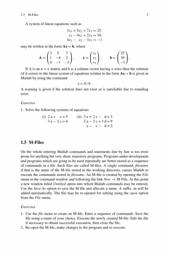
A system of linear equations such as
3x1 + 5x2 + 7x3 = 25,
x1 − 4x2 + 2x3 = 10,
4x1 − x2 − 3x3 = −1
may be written in the form Ax = b, where
A =⎛⎝
3 5 71 −4 24 −1 −3
⎞⎠ , x =
⎛⎝
x1x2x3
⎞⎠ , b =
⎛⎝
2510−1
⎞⎠ .
If A is an n × n matrix and b is a column vector having n rows then the solution(if it exists) to the linear system of equations written in the form Ax = b is given inMatlab by using the command
x = A\b
A warning is given if the solution does not exist or is unreliable due to roundingerror.
Exercises
1. Solve the following systems of equations.
(i) 2 a + c = 5 (ii) 3 a + 2 c − d = 33 a − 2 c = 4 2 a − 2 c + 3 d = 9
a − c − d = 2.
1.5 M-Files
On the whole entering Matlab commands and statements line by line is too errorprone for anything but very short, transitory programs. Programs under developmentand programs which are going to be used repeatedly are better stored as a sequenceof commands in a file. Such files are called M-files. A single command, filenameif that is the name of the M-file stored in the working directory, causes Matlab toexecute the commands stored in filename. An M-file is created by opening the Filemenu in the command window and following the link New → M-File. At this pointa new window titled Untitled opens into which Matlab commands may be entered.Use the Save As option to save the M-file and allocate a name. A suffix .m will beadded automatically. The file may be re-opened for editing using the open optionfrom the File menu.
Exercises
1. Use the file menu to create an M-file. Enter a sequence of commands. Save thefile using a name of your choice. Execute the newly created M-file. Edit the fileif necessary to obtain successful execution, then close the file.
2. Re-open the M-file, make changes to the program and re-execute.
6 1 Basic Matlab
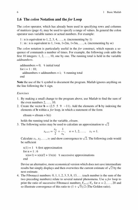
1.6 The colon Notation and the for Loop
The colon operator, which has already been used in specifying rows and columnsof matrices (page 4), may be used to specify a range of values. In general the colonoperator uses variable names or actual numbers. For example:
1 : n is equivalent to 1, 2, 3, 4, . . . , n. (incrementing by 1)1 : m : n is equivalent to 1, 1+m, 1+2m, 1+3m, . . . , n. (incrementing by m)
The colon notation is particularly useful in the for construct, which repeats a se-quence of commands a number of times. For example, the following code adds thefirst 10 integers: 1, 2, . . . , 10, one by one. The running total is held in the variableaddnumbers.
addnumbers = 0; % initial totalfor i = 1 : 10;
addnumbers = addnumbers + i; % running totalend
Note the use of the % symbol to document the program. Matlab ignores anything onthe line following the % sign.
Exercises
1. By making a small change to the program above, use Matlab to find the sum ofthe even numbers 2, . . . , 10.
2. Create the vector b = (2.5 5 9 −11). Add the elements of b by indexing theelements of b within a for loop, in which a statement of the form
eltsum = eltsum + b(i)
holds the running total in the variable, eltsum.3. The following series may be used to calculate an approximation to
√2
xn+1 = xn
2+ 1
xn
, n = 1,2, . . . , x1 = 1.
Calculate x1, x2, . . . , x7 and show convergence to√
2. The following code wouldbe sufficient
x(1) = 1 % first approximationfor n = 1 : 6
x(n+1) = x(n)/2 + 1/x(n) % successive approximationsend
Devise an alternative, more economical version which does not save intermediateresults but simply displays and then overwrites the current estimate of
√2 by the
next estimate.4. The Fibonacci numbers: 0,1,1,2,3,5,8,13, . . . (each number is the sum of the
two preceding numbers) relate to several natural phenomena. Use a for loop toprint the ratio of successive Fibonacci numbers Fn+1/Fn for n = 2, . . . ,20 andso illustrate convergence of this ratio to (1 + √
5)/2 (The Golden ratio).
1.7 The if Construct 7
Note By default Matlab continues printing until a program is completed. To viewoutput page by page enter the command more on. To restore the default enter more.
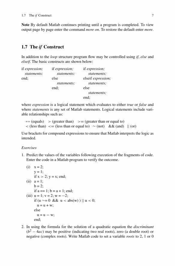
1.7 The if Construct
In addition to the loop structure program flow may be controlled using if, else andelseif. The basic constructs are shown below:
if expression; if expression; if expression;statements; statements; statements;
end; else elseif expression;statements; statements;
end; elsestatements;
end;
where expression is a logical statement which evaluates to either true or false andwhere statements is any set of Matlab statements. Logical statements include vari-able relationships such as:
== (equals) > (greater than) >= (greater than or equal to)< (less than) <= (less than or equal to) ∼ (not) && (and) || (or)
Use brackets for compound expressions to ensure that Matlab interprets the logic asintended.
Exercises
1. Predict the values of the variables following execution of the fragments of code.Enter the code in a Matlab program to verify the outcome.
(i) x = 2;y = 1;if x > 2; y = x; end;
(ii) a = 1;b = 2;if a == 1; b = a + 1; end;
(iii) u = 1; v = 2; w = −2;if (u ∼= 0 && u < abs(w) ) || u < 0;
u = u + w;else
u = u − w;end;
2. In using the formula for the solution of a quadratic equation the discriminant(b2 − 4ac) may be positive (indicating two real roots), zero (a double root) ornegative (complex roots). Write Matlab code to set a variable roots to 2, 1 or 0

8 1 Basic Matlab
depending on the value of the discriminant. Test the program using various val-ues of a, b and c.
3. Given a vector (or matrix) of dimension (m, n) use a for loop within a for loop tocount the number of non-zero elements. Test your code on simple examples.
Note the function size may be used to determine the dimensions of an array. Forexample [ n m ] = size(A) returns the number of rows, n and the number ofcolumns, m.
1.8 The while Loop
The while loop repeats a sequence of instructions until a specified condition is met.It is used as an alternative to the for loop in cases where the number of requiredrepeats is not known in advance. The basic construct is:
while expressionMatlab commands
end;
If expression evaluates to true the Matlab commands are executed and the programreturns to re-evaluating expression. If expression evaluates to false the commandfollowing end; (if any) is executed.
Exercises
1. Although a for loop would be more appropriate, enter the following code whichuses a while loop to find the sum of the numbers 1, . . . , 10.
addnumbers = 0; % set running total to 0n = 1; % first numberwhile n <= 10
addnumbers = addnumbers + n; % add current number to running totaln = n + 1; % next number
end;addnumbers % show the result
2. Create a vector of numbers which includes one or more zeros. Construct a whileloop to find the sum of the numbers up to the first zero.
3. Use a while loop and the previously quoted series to calculate an approximationto
√2 accurate to 4 decimal places by terminating the loop when the difference
between successive estimates is less than 0.00005.
Note Enter Ctrl C from the keyboard to terminate execution prematurely (useful ifa program runs out of control).
1.9 Simple Screen Output 9
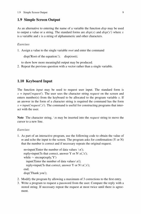
1.9 Simple Screen Output
As an alternative to entering the name of a variable the function disp may be usedto output a value or a string. The standard forms are disp(x) and disp('s ') where x
is a variable and s is a string of alphanumeric and other characters.
Exercises
1. Assign a value to the single variable root and enter the command
disp('Root of the equation:'); disp(root);
to show how more meaningful output may be produced.2. Repeat the previous question with a vector rather than a single variable.
1.10 Keyboard Input
The function input may be used to request user input. The standard form isx = input('request'). The user sees the character string request on the screen andenters number(s) from the keyboard to be allocated to the program variable x. Ifan answer in the form of a character string is required the command has the formx = input('request','s'). The command is useful for constructing programs that inter-act with the user.
Note The character string, \n may be inserted into the request string to move thecursor to a new line.
Exercises
1. As part of an interactive program, use the following code to obtain the value ofm and echo the input to the screen. The program asks for confirmation (Y or N)that the number is correct and if necessary repeats the original request.
m=input('Enter the number of data values \n');reply=input('Is that correct, answer Y or N\n','s');while ∼ strcmp(reply,'Y')
input('Enter the number of data values\n');reply=input('Is that correct, answer Y or N\n','s');
end;disp('Thank you');
2. Modify the program by allowing a maximum of 3 corrections to the first entry.3. Write a program to request a password from the user. Compare the reply with a
stored string. If necessary repeat the request at most twice until there is agree-ment.
10 1 Basic Matlab
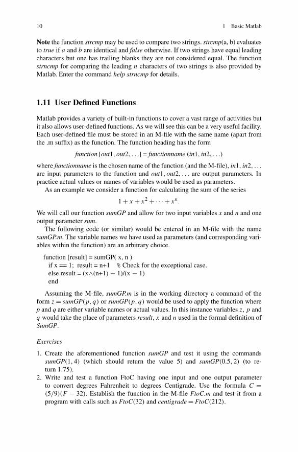
Note the function strcmp may be used to compare two strings. strcmp(a, b) evaluatesto true if a and b are identical and false otherwise. If two strings have equal leadingcharacters but one has trailing blanks they are not considered equal. The functionstrncmp for comparing the leading n characters of two strings is also provided byMatlab. Enter the command help strncmp for details.
1.11 User Defined Functions
Matlab provides a variety of built-in functions to cover a vast range of activities butit also allows user-defined functions. As we will see this can be a very useful facility.Each user-defined file must be stored in an M-file with the same name (apart fromthe .m suffix) as the function. The function heading has the form
function [out1,out2, . . .] = functionname (in1, in2, . . .)
where functionname is the chosen name of the function (and the M-file), in1, in2, . . .
are input parameters to the function and out1,out2, . . . are output parameters. Inpractice actual values or names of variables would be used as parameters.
As an example we consider a function for calculating the sum of the series
1 + x + x2 + · · · + xn.
We will call our function sumGP and allow for two input variables x and n and oneoutput parameter sum.
The following code (or similar) would be entered in an M-file with the namesumGP.m. The variable names we have used as parameters (and corresponding vari-ables within the function) are an arbitrary choice.
function [result] = sumGP( x, n )if x == 1; result = n+1 % Check for the exceptional case.else result = (x∧(n+1) − 1)/(x − 1)end
Assuming the M-file, sumGP.m is in the working directory a command of theform z = sumGP(p, q) or sumGP(p, q) would be used to apply the function wherep and q are either variable names or actual values. In this instance variables z, p andq would take the place of parameters result, x and n used in the formal definition ofSumGP.
Exercises
1. Create the aforementioned function sumGP and test it using the commandssumGP(1,4) (which should return the value 5) and sumGP(0.5,2) (to re-turn 1.75).
2. Write and test a function FtoC having one input and one output parameterto convert degrees Fahrenheit to degrees Centigrade. Use the formula C =(5/9)(F − 32). Establish the function in the M-file FtoC.m and test it from aprogram with calls such as FtoC(32) and centigrade = FtoC(212).
1.12 Basic Statistics 11
3. Write a function MaxElement to find the largest absolute value of all elements ofan array or vector. Test the function on simple examples. Note that for a given ma-trix or vector, A the Matlab function max applied to abs(A), as in max(abs(A))
would produce the same result.
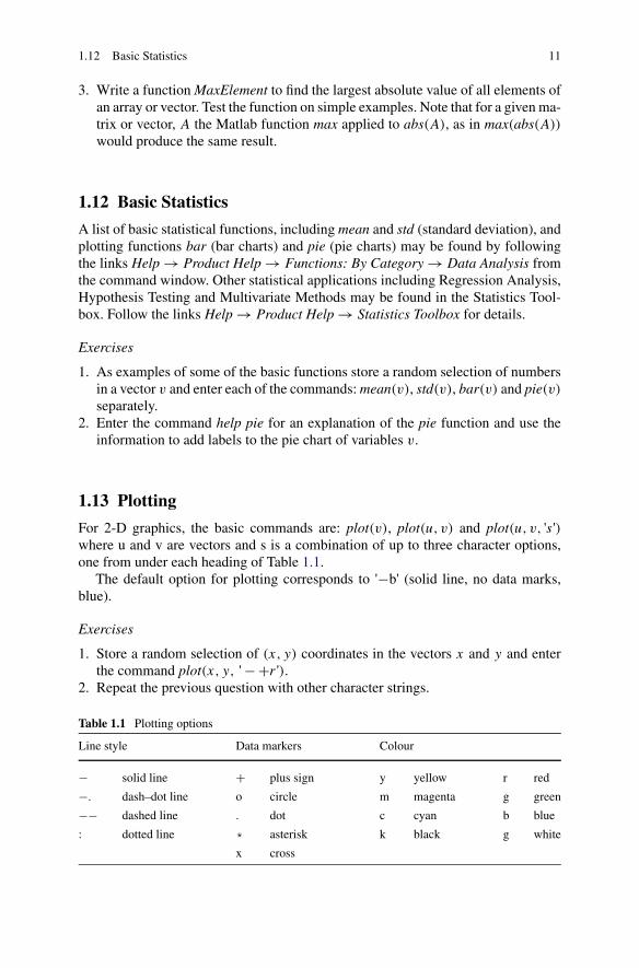
1.12 Basic Statistics
A list of basic statistical functions, including mean and std (standard deviation), andplotting functions bar (bar charts) and pie (pie charts) may be found by followingthe links Help → Product Help → Functions: By Category → Data Analysis fromthe command window. Other statistical applications including Regression Analysis,Hypothesis Testing and Multivariate Methods may be found in the Statistics Tool-box. Follow the links Help → Product Help → Statistics Toolbox for details.
Exercises
1. As examples of some of the basic functions store a random selection of numbersin a vector v and enter each of the commands: mean(v), std(v), bar(v) and pie(v)
separately.2. Enter the command help pie for an explanation of the pie function and use the
information to add labels to the pie chart of variables v.
1.13 Plotting
For 2-D graphics, the basic commands are: plot(v), plot(u, v) and plot(u, v, 's ')where u and v are vectors and s is a combination of up to three character options,one from under each heading of Table 1.1.
The default option for plotting corresponds to '−b' (solid line, no data marks,blue).
Exercises
1. Store a random selection of (x, y) coordinates in the vectors x and y and enterthe command plot(x, y, ' − +r ').
2. Repeat the previous question with other character strings.
Table 1.1 Plotting options
Line style Data markers Colour
− solid line + plus sign y yellow r red
−. dash–dot line o circle m magenta g green
−− dashed line . dot c cyan b blue
: dotted line * asterisk k black g white
x cross
12 1 Basic Matlab
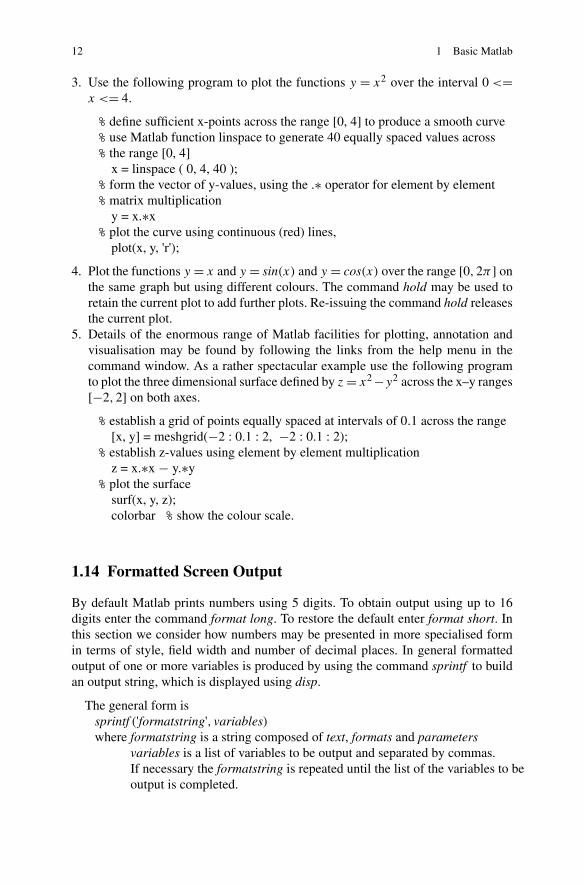
3. Use the following program to plot the functions y = x2 over the interval 0 <=x <= 4.
% define sufficient x-points across the range [0, 4] to produce a smooth curve% use Matlab function linspace to generate 40 equally spaced values across% the range [0, 4]
x = linspace ( 0, 4, 40 );% form the vector of y-values, using the .∗ operator for element by element% matrix multiplication
y = x.∗x% plot the curve using continuous (red) lines,
plot(x, y, 'r');
4. Plot the functions y = x and y = sin(x) and y = cos(x) over the range [0,2π] onthe same graph but using different colours. The command hold may be used toretain the current plot to add further plots. Re-issuing the command hold releasesthe current plot.
5. Details of the enormous range of Matlab facilities for plotting, annotation andvisualisation may be found by following the links from the help menu in thecommand window. As a rather spectacular example use the following programto plot the three dimensional surface defined by z = x2 −y2 across the x–y ranges[−2,2] on both axes.
% establish a grid of points equally spaced at intervals of 0.1 across the range[x, y] = meshgrid(−2 : 0.1 : 2, −2 : 0.1 : 2);
% establish z-values using element by element multiplicationz = x.∗x − y.∗y
% plot the surfacesurf(x, y, z);colorbar % show the colour scale.
1.14 Formatted Screen Output
By default Matlab prints numbers using 5 digits. To obtain output using up to 16digits enter the command format long. To restore the default enter format short. Inthis section we consider how numbers may be presented in more specialised formin terms of style, field width and number of decimal places. In general formattedoutput of one or more variables is produced by using the command sprintf to buildan output string, which is displayed using disp.
The general form issprintf ('formatstring', variables)where formatstring is a string composed of text, formats and parameters
variables is a list of variables to be output and separated by commas.If necessary the formatstring is repeated until the list of the variables to beoutput is completed.
1.14 Formatted Screen Output 13
Formats are preceded by % and are applied in the order of the variables. The moreused formats are illustrated below:
d for integer formatfor example %6d for a field width of 6 places.
f fixed point formatfor example %10.5f for a field width of 10 places and 5 decimal places.
e floating point (exponent) formatfor example %10.3e for a field width of 10 places and 3 decimal placeexponent.
We will use the parameter \n (newline) but there are others. For more details anddetails of other features of the format command, enter help format in the commandwindow.
Exercises
1. Enter the following code to compare π and its popular approximation 22/7.
ratio = 22/7;s1 = sprintf('pi to 6 decimal places is %8.6f ', pi);s2 = sprintf('22/7 to 6 decimal places is %8.6f ', ratio);disp(s1); disp(s2);
2. Repeat the previous question making use of the \n parameter to obtain the sameoutput using a single string. It may be necessary to use more that one line to enterthe format. Use the continuation mark as shown in the example below.
3. Allocate values to variables Node, ux and uy and use the following commandsto produce the output:
Node 27 ux 1.0934 uy 3.5e+005
s = sprintf( . . . % three dots indicate a continuation to the next line'Node %3d ux %6.4f uy %10.3e', Node, ux, uy);disp(s);
4. Display the matrix
A =⎛⎝
1 2 4.563 4 5.03 29 4.567
⎞⎠
noting that Matlab stores elements of a matrix in column order and so to obtainthe desired effect the transpose of A is used, for example:
s = sprintf('%6.3f %6.3f %6.3f \n ', A');disp(s);
5. Repeat the previous question but with a more detailed format so that the displayof matrix A bears a closer resemblance to the form shown above.

14 1 Basic Matlab
1.15 File Input and Output
In order to access a file it must be opened. A command of the form fid =fopen('filename', 'w+') opens a file for read, write and create access in M/S Win-dows systems (other operating systems may vary). Formats may be used for ap-pending output to an existing file. Enter the command help fopen for details. Thevariable, fid is known as a file identifier and is used by Matlab to identify the file insubsequent operations.
1.15.1 Formatted Output to a File
The command fprintf writes formatted data to a file. The structure of the commandis exactly the same as that of sprintf but with a file identifier as the first parameter.For example fprintf (fid, . . . ).
Exercises
1. Repeat any of the questions from (1.14) but print the results to a file. Display thefile after executing the formatting code using the command type filename.
Use the following code as an example which opens and writes to a Windowsfile myfile.txt. If the file already exists it is overwritten.
fid = fopen('myfile.txt','w+');fprintf(fid, 'pi to 6 decimal places is %8.6f ', pi);type myfile.txt
1.15.2 Formatted Input from a File
There are other commands for reading formatted input from a file but textscan is par-ticularly useful as it does not require the precise specification of incoming formats.For example to read a line of the form
Node 27 ux 1.0934 uy 3.5e+005textscan only requires the information
%s %d %s %f %s %fwhere %s denotes a character string, %d denotes an integer and %f denotes a fixed orfloating point number. Other formats are available.
Exercises
1. Create a file data.txt with first line:
Node 27 ux 1.0934 uy 3.5e+005
1.15 File Input and Output 15
Enter the code shown below to open the file, read the data and allocate thenumbers to program variables a, b and c. The function textscan produces out-put in a Matlab cell, which differs from an array in that elements of differentsizes and different types may be stored. In this example the name mydata hasbeen chosen for the cell, output corresponding to each item in the format stringis placed in successive positions of mydata. Whereas items from a matrix are re-trieved using enclosing ( and ) parentheses, items from a cell are retrieved usingthe pair { and }.
fid = fopen('data.txt');mydata = textscan(fid, ' %s %d %s %f %s %f ')% retrieve the numbers 27, 1.0934 and 3.5e+005% the strings Node, ux and uy will be held in mydata{1}, mydata{3} and% mydata{5}a = mydata{2}b = mydata{4}c = mydata{6}
The function textscan may be used to collect data from several consecutive linesof data provided the stated format applies. To limit the number of lines that textscanreads for a given format a third parameter is available. A command of the formtextscan(fid, format, n) would apply the format n times from the current position.A command frewind(fid) is available to re-set the internal pointer to start of the file.
A further feature of textscan allows unwanted data to be skipped by insertingan ∗ between the relevant % and the following s, d or f in the format string.
Exercises
1. Add a few more lines of similar data to the file mydata. Use a single textscancommand to read the whole file and notice how the data is retrieved as columnvectors.
2. Modify the format string of the previous question. Choose a selection of columnsof the data file to be retrieved.
1.15.3 Unformatted Input and Output (Saving and RetrievingData)
Workspace variables may be stored more economically as unformatted data (data inbinary form and as such impossible to read with the human eye) in a file having aname with a .mat suffix. Use the commands save to save and load to restore.
For example the command save('savedata.mat', 'x ', 'y ', 'z') would store variablesx, y, z in the file savedata.mat and load('savedata.mat', 'x ', 'y ', 'z') would re-loadthe variables. The commands save and load without parameters save and load allworkspace variables.

16 1 Basic Matlab
Exercises
1. Assign variables to matrices A and B. Save the matrices in unformatted form toa .mat file.
2. Clear A and B from the workspace using the command clear A B. Check thatthey no longer exist.
3. Retrieve the matrices A and B from the .mat file. Check that nothing has beenlost.
Chapter 2Linear Equations
Aims In this chapter we look at ways of solving systems of linear equations,sometimes known as simultaneous linear equations. We investigate
• Gaussian elimination and its variants, to obtain a solution to a system.• partial pivoting within Gaussian elimination, to improve the accuracy of the re-
sults.• iterative refinement after Gaussian elimination, to improve the accuracy of a first
solution.
In some circumstances the use of Gaussian elimination is not recommended andother techniques based on iteration are more appropriate including
• Gauss–Seidel iteration.
We look at the method in detail and compare this iterative technique with directsolvers based on elimination.
Overview We begin by examining what is meant by a linear relationship, beforeconsidering how to handle the (linear) equations which represent such relationships.We describe methods for finding a solution, which simultaneously satisfies severalsuch linear equations. In so doing we identify situations for which we can guaranteethe existence of one, and only one, solution; situations for which more than onesolution is possible; and situations for which there may be no solution at all.
As already indicated, the methods to be considered neatly fall into two categories;direct methods based on elimination; and iterative techniques. We look at each typeof method in detail. For direct methods we need to bear in mind the limitations ofcomputer arithmetic, and hence we consider how best to implement the methods sothat as the algorithm proceeds the accumulation of error may be kept to a minimum.For iterative methods the concern is more related to ensuring that convergence to aspecified accuracy is achieved in as few iterations as possible.
Acquired Skills After reading this chapter you will appreciate that solving lin-ear equations is not as straightforward a matter as might appear. No matter which
C. Woodford, C. Phillips, Numerical Methods with Worked Examples: Matlab Edition,DOI 10.1007/978-94-007-1366-6_2, © Springer Science+Business Media B.V. 2012
17
18 2 Linear Equations
method you use accumulated computer errors may make the true solution unattain-able. However you will be equipped with techniques to identify the presence ofsignificant errors and to take avoiding action. You will be aware of the differencesbetween a variety of direct and indirect methods and the circumstances in which theuse of a particular method is appropriate.
2.1 Introduction
One of the simplest ways in which a physical entity may be seen to behave is to varyin a linear manner with respect to some external influence. For example, the length(L) of the mercury column in a thermometer is accepted as being directly related toambient temperature (T ); an increase in temperature is shown by a correspondingincrease in the length of the column. This linear relationship may be expressed as
L = kT + c.
Here k and c are constants whose values depend on the units in which temperature(degrees Celsius, Fahrenheit, etc.) and length (millimetres, inches, etc.) are mea-sured, and on the bore of the tube. k represents the change in length relative to a risein temperature, whilst c corresponds to the length of the column at zero degrees.We refer to T as the independent variable and L as the dependent variable. If wewere to plot values of L against corresponding values of T we would have a straightline with slope k and intercept on the L axis equal to c.
A further example of a linear relationship is Hooke’s Law (2.1) which relates thetension in a spring to the length by which it has been extended. If T is the tension,x is the extension of the spring, a is the unextended length and λ is the modulus ofelasticity, then we have
T = λ
ax. (2.1)
Typical units are Newtons (for T and λ) and metres (for x and a). A plot of T
against x would reveal a straight line passing through the origin with slope λ/a.An example which involves more than two variables is supplied by Kirchoff’s
Law which states that the algebraic sum of currents meeting at a point must be zero.Hence, if i1, i2 and i3 represent three such currents, we must have
i1 + i2 + i3 = 0. (2.2)
An increase in the value of one of the variables (say i1) must result in a correspond-ing decrease (to the same combined value) in one or more of the other two variables(i2 and/or i3) and in this sense the relationship is linear. For a relationship to be lin-ear, the variables (or constant multiples of the variables) are combined by additionsand subtractions.
2.2 Linear Systems 19
2.2 Linear Systems
In more complicated modelling situations it may be that there are many linear re-lationships, each involving a large number of variables. For example, in the stressanalysis of a structure such as a bridge or an aeroplane, many hundreds (or indeedthousands) of linear relationships may be involved. Typically, we are interested indetermining values for the dependent variables using these relationships so that wecan answer the following questions:
• For a given extension of a spring, what is the tension?• If one current has a specific value, what values for the remaining currents ensure
that Kirchoff’s Law is preserved?• Is a bridge able to withstand a given level of traffic?
As an example of a linear system consider a sporting event where spectators werecharged for admission at the rate of £15.50 for adults and £5.00 for concessions. It isknown that the total takings for the event was £3312 and that a total of 234 spectatorswere admitted to the event. The problem is to determine how many adults watchedthe event.
If we let x represent the number of adults and y the number of concessions thenwe know that the sum of x and y must equal 234, the total number of spectators.Further, the sum of 15.5x and 5y must equal 3312, the total takings. Expressed inmathematical notation, we have
x + y = 234 (2.3)
15.5x + 5y = 3312. (2.4)
Sets of equations such as (2.3) and (2.4) are known as systems of linear equationsor linear systems. It is an important feature of this system, and other systems weconsider in this chapter, that the number of equations is equal to the number ofunknowns to be found.
When the number of equations (and consequently the number of variables inthose equations) becomes large it can be tedious to write the system out in full. Inany case, we need some notation which will allow us to specify an arbitrary linearsystem in compact form so that we may conveniently examine ways of solving sucha system. Hence we write linear systems using matrix and vector notation as
Ax = b (2.5)
where A is a matrix, known as the coefficient matrix (or matrix of coefficients),b is the vector of right-hand sides and x is the vector of unknowns to be determined.Assuming n (the length of x) unknowns to be determined, b must be an n-columnvector and A an m × n square matrix, although for the time being we only considersystems with the same number of equations as unknowns, (m = n).
Problem
Write (2.3), (2.4) in matrix–vector form.
20 2 Linear Equations
Solution
We have
Ax = b, where A =(
1 115.5 5
), x =
⎧⎪⎪⎩x
y
⎫⎪⎪⎭ , b =⎧⎪⎪⎩ 234
3312
⎫⎪⎪⎭ .
A great number of electronic, mechanical, economic, manufacturing and naturalprocesses may be modelled using linear systems in which, as in the above simpleexample, the number of unknowns matches the number of equations. If, as some-times happens, the modelling process results in nonlinear equations (equations in-volving perhaps squares, exponentials or products of the unknowns) it is often thecase that the iterative techniques involved to solve these systems reduce to findingthe solution of a linear system at each iteration. Hence linear equation solvers havea wider applicability than might at first appear to be the case.
Since the modelling process either directly or indirectly yields a system of linearequations, the ability to solve such systems is fundamental. Our interest is in meth-ods which can be implemented in a computer program and so we must bear in mindthe limitations of computer arithmetic.
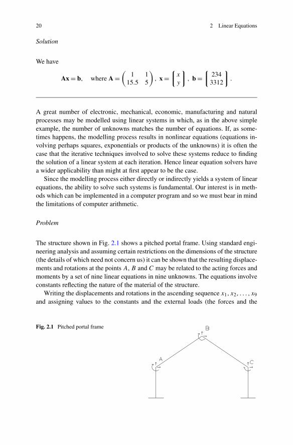
Problem
The structure shown in Fig. 2.1 shows a pitched portal frame. Using standard engi-neering analysis and assuming certain restrictions on the dimensions of the structure(the details of which need not concern us) it can be shown that the resulting displace-ments and rotations at the points A, B and C may be related to the acting forces andmoments by a set of nine linear equations in nine unknowns. The equations involveconstants reflecting the nature of the material of the structure.
Writing the displacements and rotations in the ascending sequence x1, x2, . . . , x9
and assigning values to the constants and the external loads (the forces and the
Fig. 2.1 Pitched portal frame
2.2 Linear Systems 21
moments) we might find that in a particular instance the equations take the followingform:
x1 = 0 (2.6)
x2 = 10 (2.7)
2x3 − 10x5 + 3x6 = 5 (2.8)
3x4 − 2x5 + 2x6 − 3x7 = 2 (2.9)
x5 + 5x6 + x7 = 14 (2.10)
3x6 − 4x7 = 17 (2.11)
2x7 = −4 (2.12)
2x8 = 10 (2.13)
x9 = 1. (2.14)
Solution
Although this is quite a large system we can take advantage of its special structureto obtain a solution fairly easily. From (2.14) that x9 = 1, from (2.13) that x8 = 5,and from (2.12) that x7 = −2.
To obtain the rest of the solution values we make use of the values that we alreadyknow. Substituting the value of x7 into (2.11) we have 3x6 + 8 = 17 and so x6 = 3.Now that we know x6 and x7 we can reduce (2.10) to an equation involving x5 only,to give x5 + 15 − 2 = 14, and so x5 = 1. Similarly we can determine x4 from (2.9)using 3x4 − 2 + 6 + 6 = 2, to give x4 = −2 2
3 . Finally, to complete the solution wesubstitute the known values for x5 and x6 into (2.8) to obtain 2x3 − 10 + 9 = 5 andconclude that x3 = 3. From (2.7) and (2.6) we have x2 = 10 and x1 = 0 to completethe solution.
To summarise, we have x1 = 0, x2 = 10, x3 = 3, x4 = −2 23 , x5 = 1, x6 = 3,
x7 = −2, x8 = 5 and x9 = 1.
Discussion
The system of equations we have just solved is an example of an upper triangularsystem. If we were to write the system in the matrix and vector form Ax = b, Awould be an upper triangular matrix, that is a matrix with zero entries below thediagonal. Mathematically the matrix A is upper triangular if for all elements aij
aij = 0, i > j.
For systems in which the coefficient matrix is upper triangular the last equation inthe system is easily solved and this value can then be used to solve the penultimateequation. The results from these last two equations may be used to solve the previousequation, and so on. In this manner the whole system may be solved. The process ofworking backwards to complete the solution is known as backward substitution.
22 2 Linear Equations
2.3 Gaussian Elimination
As part of the process we consider how general linear systems may be solved byreduction to upper triangular form.
Problem
Find the numbers of adults and concessions at the sporting event (2.3), (2.4) bysolving the system of two equations in two unknowns.
Solution
In subtracting 15.5 times (2.3) from (2.4) we have 1.5y = 91.5, and combining thiswith the original first equation we have
x + y = 234 (2.15)
−10.5y = −315 (2.16)
which is in upper triangular form. Solving (2.16) gives y = 30 (concessions) andsubstituting this value into (2.15) gives x = 234 − 30 = 204 (adults).
Discussion
The example illustrates an important mechanism for determining the solution toa system of equations in two unknowns, which may readily be extended to largersystems. It has two components:
1. Transform the system of equations into an equivalent one (that is, the solution tothe transformed system is mathematically identical to the solution to the originalsystem) in which the coefficient matrix is upper triangular.
2. Solve the transformed problem using backward substitution.
A linear system may be reduced to upper triangular form by means of successivelysubtracting multiples of the first equation from the second, third, fourth and so on,then repeating the process using multiples of the newly-formed second equation,and again with the newly-formed third equation, and so on until the penultimateequation has been used in this way. Having reduced the system to upper triangularform backward substitution is used to find the solution. This systematic approach,known as Gaussian elimination, is illustrated further in the following example.
Problem
Solve the following system of four equations in four unknowns
2.3 Gaussian Elimination 23
2x1 + 3x2 + 4x3 − 2x4 = 1 (2.17)
x1 − 2x2 + 4x3 − 3x4 = 2 (2.18)
4x1 + 3x2 − x3 + x4 = 2 (2.19)
3x1 − 4x2 + 2x3 − 2x4 = 5. (2.20)
Solution
As a first step towards an upper triangular system we eliminate x1 from (2.18), (2.19)and (2.20). To do this we subtract 1/2 times (2.17) from (2.18), 2 times (2.17) from(2.19), and 3/2 times (2.17) from (2.20). In each case the fraction involved in themultiplication (the multiplier) is the ratio of two coefficients of the variable beingeliminated from (2.18)–(2.20). The numerator is the coefficient of the variable tobe eliminated and the denominator is the coefficient of that variable in the equationwhich is to remain unchanged. As a result of these computations the original systemis transformed into
2x1 + 3x2 + 4x3 − 2x4 = 1 (2.21)
− 72x2 + 2x3 − 2x4 = 3
2 (2.22)
− 3x2 − 9x3 + 5x4 = 0 (2.23)
− 172 x2 − 4x3 + x4 = 7
2 . (2.24)
To proceed we ignore (2.21) and repeat the process on (2.22)–(2.24). We elimi-nate x2 from (2.23) and (2.24) by subtracting suitable multiples of (2.22). We take(−3)/(− 7
2 ) times (2.22) from (2.23) and (−17)/(−7) times (2.22) from (2.24) togive (after the removal of common denominators) the system
2x1 + 3x2 + 4x3 − 2x4 = 1 (2.25)
− 72x2 + 2x3 − 2x4 = 3
2 (2.26)
− 757 x3 + 47
7 x4 = − 97 (2.27)
− 627 x3 + 41
7 x4 = − 17 . (2.28)
Finally we subtract 62/75 times (2.27) from (2.28) to give the system
2x1 + 3x2 + 4x3 − 2x4 = 1 (2.29)
− 72x2 + 4x3 − 2x4 = 3
2 (2.30)
− 757 x3 + 47
7 x4 = − 97 (2.31)
161525x4 = − 483
525 . (2.32)
We now have an upper triangular system which may be solved by backward substi-tution. From (2.32) we have x4 = 3. Substituting this value in (2.31) gives x3 = 2.Substituting the known values for x4 and x3 in (2.30) gives x2 = −1. Finally us-ing (2.29) we find x1 = 1. The extension of Gaussian elimination to larger systems
24 2 Linear Equations
is straightforward. The aim, as before, is to transform the original system to uppertriangular form which is solved by backward substitution.
Discussion
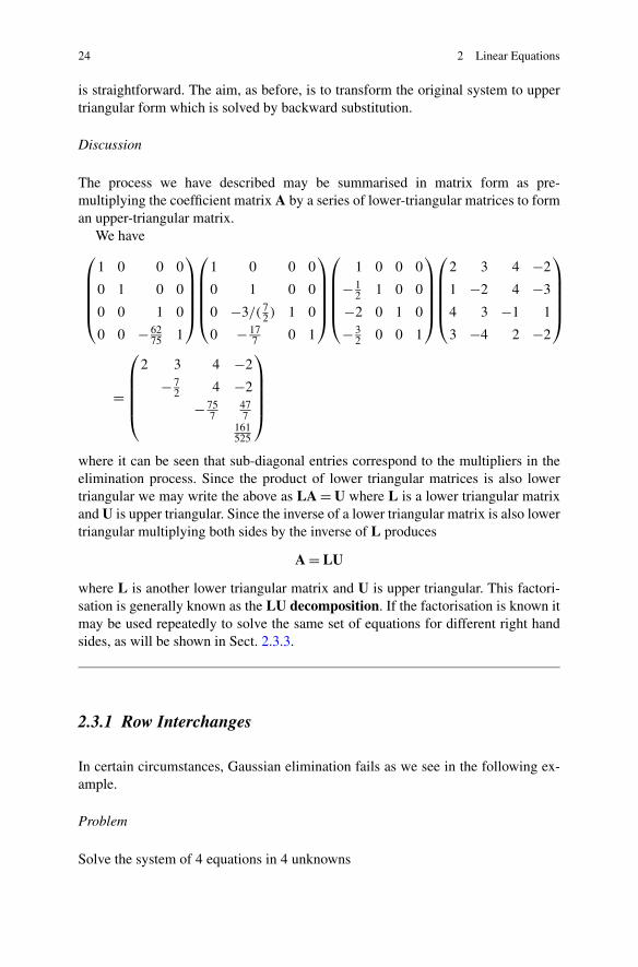
The process we have described may be summarised in matrix form as pre-multiplying the coefficient matrix A by a series of lower-triangular matrices to forman upper-triangular matrix.
We have⎛⎜⎜⎜⎜⎝
1 0 0 0
0 1 0 0
0 0 1 0
0 0 − 6275 1
⎞⎟⎟⎟⎟⎠
⎛⎜⎜⎜⎜⎝
1 0 0 0
0 1 0 0
0 −3/( 72 ) 1 0
0 − 177 0 1
⎞⎟⎟⎟⎟⎠
⎛⎜⎜⎜⎜⎝
1 0 0 0
− 12 1 0 0
−2 0 1 0
− 32 0 0 1
⎞⎟⎟⎟⎟⎠
⎛⎜⎜⎜⎜⎝
2 3 4 −2
1 −2 4 −3
4 3 −1 1
3 −4 2 −2
⎞⎟⎟⎟⎟⎠
=
⎛⎜⎜⎜⎜⎝
2 3 4 −2
− 72 4 −2
− 757
477
161525
⎞⎟⎟⎟⎟⎠
where it can be seen that sub-diagonal entries correspond to the multipliers in theelimination process. Since the product of lower triangular matrices is also lowertriangular we may write the above as LA = U where L is a lower triangular matrixand U is upper triangular. Since the inverse of a lower triangular matrix is also lowertriangular multiplying both sides by the inverse of L produces
A = LU
where L is another lower triangular matrix and U is upper triangular. This factori-sation is generally known as the LU decomposition. If the factorisation is known itmay be used repeatedly to solve the same set of equations for different right handsides, as will be shown in Sect. 2.3.3.
2.3.1 Row Interchanges
In certain circumstances, Gaussian elimination fails as we see in the following ex-ample.
Problem
Solve the system of 4 equations in 4 unknowns

2.3 Gaussian Elimination 25
2x1 − 6x2 + 4x3 − 2x4 = 8 (2.33)
x1 − 3x2 + 4x3 + 3x4 = 6 (2.34)
4x1 + 3x2 − 2x3 + 3x4 = 3 (2.35)
x1 − 4x2 + 3x3 + 3x4 = 9. (2.36)
Solution
To eliminate x1 from (2.34), (2.35) and (2.36) we take multiples 12 , 2 and 1
2 of(2.33) and subtract from (2.34), (2.35) and (2.36) respectively. We now have thelinear system
2x1 − 6x2 + 4x3 − 2x4 = 8
2x3 + 4x4 = 2 (2.37)
15x2 − 10x3 + 7x4 = −13 (2.38)
− x2 + x3 + 4x4 = 5. (2.39)
Since x2 does not appear in (2.37) we are unable to proceed as before. However asimple re-ordering of the equations enables x2 to appear in the second equation ofthe system and this permits further progress. Exchanging (2.37) and (2.38) we havethe system
2x1 − 6x2 + 4x3 − 2x4 = 8
15x2 − 10x3 + 7x4 = −13 (2.40)
2x3 + 4x4 = 2
− x2 + x3 + 4x4 = 5. (2.41)
Resuming the elimination procedure we eliminate x2 from (2.41) by taking a multi-ple (−1)/15 of (2.40) from (2.41) to give
2x1 − 6x2 + 4x3 − 2x4 = 8
15x2 − 10x3 + 7x4 = −13
2x3 + 4x4 = 2 (2.42)13x3 + 67
15x4 = 6215 . (2.43)
Finally, to eliminate x3 from (2.43) we take a multiple 1/6 of (2.42) from (2.43). Asa result we now have the linear system
2x1 − 6x2 + 4x3 − 2x4 = 8
15x2 − 10x3 + 7x4 = −13
2x3 + 4x4 = 25715x4 = 57
15 ,
which is an upper triangular system that can be solved by backward substitution togive the solution x4 = 1, x3 = −1, x2 = −2, and x1 = 1.
26 2 Linear Equations
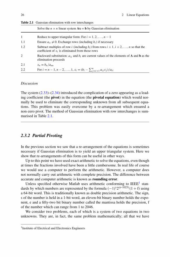
Table 2.1 Gaussian elimination with row interchanges
Solve the n × n linear system Ax = b by Gaussian elimination
1 Reduce to upper triangular form: For i = 1,2, . . . , n − 1
1.1 Ensure aii �= 0. Exchange rows (including bi ) if necessary
1.2 Subtract multiples of row i (including bi ) from rows i + 1, i + 2, . . . , n so that thecoefficient of xi is eliminated from those rows
2 Backward substitution: aij and bi are current values of the elements of A and b as theelimination proceeds
2.1 xn = bn/ann
2.2 For i = n − 1, n − 2, . . . ,1, xi = (bi − ∑nj=i+1 aij xj )/aii
Discussion
The system (2.33)–(2.34) introduced the complication of a zero appearing as a lead-ing coefficient (the pivot) in the equation (the pivotal equation) which would nor-mally be used to eliminate the corresponding unknown from all subsequent equa-tions. This problem was easily overcome by a re-arrangement which ensured anon-zero pivot. The method of Gaussian elimination with row interchanges is sum-marised in Table 2.1.
2.3.2 Partial Pivoting
In the previous section we saw that a re-arrangement of the equations is sometimesnecessary if Gaussian elimination is to yield an upper triangular system. Here weshow that re-arrangements of this form can be useful in other ways.
Up to this point we have used exact arithmetic to solve the equations, even thoughat times the fractions involved have been a little cumbersome. In real life of coursewe would use a computer to perform the arithmetic. However, a computer doesnot normally carry out arithmetic with complete precision. The difference betweenaccurate and computer arithmetic is known as rounding error.
Unless specified otherwise Matlab uses arithmetic conforming to IEEE1 stan-dards by which numbers are represented by the formula (−1)s2(e-1023)(1 + f) usinga 64-bit word. This is traditionally known as double precision arithmetic. The sign,s of the number is held in a 1-bit word, an eleven-bit binary number holds the expo-nent, e and a fifty-two bit binary number called the mantissa holds the precision, fof the number which can range from 1 to 2046.
We consider two problems, each of which is a system of two equations in twounknowns. They are, in fact, the same problem mathematically; all that we have
1Institute of Electrical and Electronics Engineers
2.3 Gaussian Elimination 27
done is to reverse the order of the two equations. The solution can be seen to bex1 = 1, x2 = 1. To illustrate the effect of rounding error we consider the followingproblem.
Problem
Solve the following systems rounding the results of all arithmetic operations to threesignificant figures.
System (1):
0.124x1 + 0.537x2 = 0.661 (2.44)
0.234x1 + 0.996x2 = 1.23 (2.45)
System (2):
1.234x1 + 0.996x2 = 1.23 (2.46)
0.124x1 + 0.537x2 = 0.661. (2.47)
Solution
• System (1): In the usual manner we eliminate x2 from (2.45) by subtracting theappropriate multiple of (2.44). In this case the multiple is 0.234/0.124 which,rounded to three significant figures, is 1.89. Multiplying 0.537 by 1.89 gives 1.01and subtracting this from 0.996 gives −0.0140. Similarly for the right-hand sideof the system, 0.661 multiplied by 1.89 is 1.25 and when subtracted from 1.23gives −0.0200. The system in its upper triangular form is
0.124x1 + 0.537x2 = 0.661 (2.48)
− 0.014x2 = −0.020. (2.49)
In backward substitution, x2 is obtained from 0.0200.014 to give 1.43 which is used in
(2.48) to give x1 = −0.863. In this case the solution obtained by using arithmeticwhich retains three significant figures is nothing like the true solution.
• System (2): We eliminate x2 from (2.47) by subtracting the appropriate mul-tiple of (2.46). In this case the multiple is 0.124/0.234, which is 0.530 tothree significant figures. Multiplying 0.537 by 0.530 and subtracting from 0.996gives 0.00900. Multiplying 0.661 by 0.530 and subtracting from 1.23 also gives0.00900 and so the system in upper triangular form is
0.234x1 + 0.996x2 = 1.23
0.009x2 = 0.009.
By backward substitution we have x2 = 1.00, followed by x1 = 1.00 which is theexact solution.
28 2 Linear Equations
Discussion
We can infer from these two simple examples that the order in which equations arepresented can have a significant bearing on the accuracy of the computed solution.The example is a little artificial, given that a modern computer carries out its arith-metic to many more significant figures than the three we have used here, often asmany as sixteen or more. Nevertheless, for larger systems it may be verified that theorder in which the equations are presented has a bearing on the accuracy of a com-puter solution obtained using Gaussian elimination. The next example describes astrategy for rearranging the equations within Gaussian elimination with a view toreducing the effect of rounding errors on a computed solution. We note in passingthat an LU decomposition which takes account of partial pivoting of a non-singularmatrix A is available in the form PA = LU where L and U are lower and uppertriangular matrices and P is a permutation matrix, a matrix of zeros and ones that inpre-multiplying A performs the necessary row exchanges. For example exchangingrows 2 and 3 of a 3 × 3 matrix A may be achieved by pre-multiplying A by the
permutation matrix
(1 0 00 0 10 1 0
).
Problem
Solve the system (2.33)–(2.36) using row exchanges to minimise pivotal values ateach step of the elimination.
Solution
We recall that in obtaining the previous solution example it was necessary to rear-range the equations during the reduction to upper triangular form to avoid a zeropivot. In this example we perform similar rearrangements, not just out of neces-sity, but also with accuracy in mind. Looking down the first column we see that thelargest (in magnitude) coefficient of x1 occurs in (2.35). We thus re-order the equa-tions to make this the pivot. This involves exchanging (2.35) and (2.33). We nowhave the linear system
4x1 + 3x2 − 2x3 + 3x4 = 3 (2.50)
x1 − 3x2 + 4x3 + 3x4 = 6 (2.51)
2x1 − 6x2 + 4x3 − 2x4 = 8 (2.52)
x1 − 4x2 + 3x3 + 3x4 = 9 (2.53)
and we eliminate x1 from (2.51), (2.52) and (2.53) by subtracting multiples 14 , 2
4 and14 of (2.50) from (2.51), (2.52) and (2.53) respectively. Looking back to the system(2.33)–(2.36) we see that the multipliers without re-arrangement were 1
2 , 2 and 12 .
Now they are uniformly smaller. This will prove to be significant. At the end of this,the first stage, of elimination, the original system is transformed to
2.3 Gaussian Elimination 29
4x1 − 3x2 − 2x3 + 3x4 = 3
− 3 34x2 + 4 1
2x3 + 2 14x4 = 5 1
4 (2.54)
− 7 12x2 + 5x3 − 3 1
2x4 = 6 12 (2.55)
− 4 34x2 + 3 1
2x3 + 2 14x4 = 8 1
4 . (2.56)
Considering (2.54)–(2.56) we see that the largest coefficient of x2 occurs in (2.55).We exchange (2.55) and (2.54) to obtain
4x1 − 3x2 − 2x3 + 3x4 = 3
− 7 12x2 + 5x3 − 3 1
2x4 = 6 12 (2.57)
− 3 34x2 + 4 1
2x3 + 2 14x4 = 5 1
4 (2.58)
− 4 34x2 + 3 1
2x3 + 2 14x4 = 8 1
4 . (2.59)
To eliminate x2 from (2.58) and (2.59) we take multiples 12 and 19
30 of (2.57) andsubtract them from (2.58) and (2.59) respectively. As a result we have the linearsystem
4x1 − 3x2 − 2x3 + 3x4 = 3
− 7 12x2 + 5x3 − 3 1
2x4 = 6 12
2x3 + 4x4 = 213x3 + 4 7
15x4 = 4 215 . (2.60)
No further row interchanges are necessary since the coefficient of x3 having thelargest absolute value is already in its correct place. We eliminate x3 from (2.60)using the multiplier 1
6 and as a result we have the linear system
4x1 − 3x2 − 2x3 + 3x4 = 3
− 7 12x2 + 5x3 − 3 1
2x4 = 6 12
2x3 + 4x4 = 2
3 45x4 = 3 4
5 .
Solving by backward substitution we obtain x4 = 1.0, x3 = −1.0, x2 = −2.0, andx1 = 1.0.
Discussion
The point of this example is to illustrate the technique known as partial pivoting.At each stage of Gaussian elimination the pivotal equation is chosen to maximisethe absolute value of the pivot. Thus the multipliers in the subsequent subtractionprocess are reduced (a division by the pivot is involved) so that they are all at mostone in magnitude. Any rounding errors present are less likely to be magnified asthey permeate the rest of the calculation.
The 4 × 4 example of this section was solved on a computer using an imple-mentation of Gaussian elimination and computer arithmetic based on a 32-bit word

30 2 Linear Equations
Table 2.2 Gaussian elimination with partial pivoting
Solve the n × n linear system Ax = b by Gaussian elimination with partial pivoting
1 Reduce to upper triangular form: For i = 1,2, . . . , n − 1
1.1 Find the j from j = i, i + 1, . . . , n for which |aji | is a maximum
1.2 If i �= j exchange rows i and j (including bi and bj )
1.3 Subtract multiples of row i (including bi ) from rows i + 1, i + 2, . . . , n so that thecoefficient of xi is eliminated from those rows
2 Backward substitution: aij and bi are current values of the elements of A and b as theelimination proceeds
2.1 xn = bn/ann
2.2 For i = n − 1, n − 2, . . . ,1, xi = (bi − ∑nj=i+1 aij xj )/aii
(equivalent to retaining at least six significant figures). Without partial pivotingthe solution obtained was x1 = 1.00000, x2 = −2.00000, x3 = −0.999999, andx4 = 1.00000, whereas elimination with pivoting gave the same solution except forx3 = −1.00000. This may seem to be an insignificant improvement but the exampleillustrates how the method works. Even with 64-bit arithmetic it is confirmed byexperience that partial pivoting particularly when used in solving larger systems ofperhaps 10 or more equations is likely to be beneficial. As we will see, the form ofthe coefficient matrix can be crucial. For these reasons commercial implementationsof Gaussian elimination always employ partial pivoting. The method is summarisedin Table 2.2.
2.3.3 Multiple Right-Hand Sides
In a modelling process the right-hand side values often correspond to boundaryvalues which may, for example, be the external loads on a structure or the resourcesnecessary to fund various activities. As part of the process it is usual to experimentwith different boundary conditions in order to achieve an optimal design. Gaussianelimination may be used to solve systems having several right-hand sides with littlemore effort than that involved in solving for just one set of right-hand side values.
Problem
Find three separate solutions of the system of (2.33)–(2.36) corresponding to threedifferent right-hand sides.
Writing the system in the form Ax = b we have three different vectors b, namely⎧⎪⎪⎪⎪⎪⎪⎪⎪⎪⎩8639
⎫⎪⎪⎪⎪⎪⎪⎪⎪⎪⎭ ,
⎧⎪⎪⎪⎪⎪⎪⎪⎪⎪⎩23
−14
⎫⎪⎪⎪⎪⎪⎪⎪⎪⎪⎭ and
⎧⎪⎪⎪⎪⎪⎪⎪⎪⎪⎩1
−6−3
9
⎫⎪⎪⎪⎪⎪⎪⎪⎪⎪⎭ .
2.3 Gaussian Elimination 31
The three problems may be expressed in the following compact form
2x1 − 6x2 + 4x3 − 2x4 = 8, 2, 1
x1 − 3x2 + 4x3 + 3x4 = 6, 3,−6
4x1 + 3x2 − 2x3 + 3x4 = 3,−1,−3
x1 − 4x2 + 3x3 + 3x4 = 9, 4, 9.
Solution
We can solve all three equations at once by maintaining not one, but three columnson the right-hand side. The interchanges required by partial pivoting and the oper-ations on the coefficient matrix do not depend on the right-hand side values and soneed not be repeated unnecessarily. After the first exchange we have
4x1 + 3x2 − 2x3 + 3x4 = 3,−1,−3
x1 − 3x2 + 4x3 + 3x4 = 6, 3,−6
2x1 − 6x2 + 4x3 − 2x4 = 8, 2, 1
x1 − 4x2 + 3x3 + 3x4 = 9, 4, 9
followed by
4x1 − 3x2 − 2x3 + 3x4 = 3, −1, −3
− 3 34x2 + 4 1
2x3 + 2 14x4 = 5 1
4 , 3 14 , −5 1
4
− 7 12x2 + 5x3 − 3 1
2x4 = 6 12 , 2 1
2 , 2 12
− 4 34x2 + 3 1
2x3 + 2 14x4 = 8 1
4 , 4 14 , 9 3
4 .
Continuing the elimination we obtain
4x1 − 3x2 − 2x3 + 3x4 = 3, −1, −3
− 7 12x2 + 5x3 − 3 1
2x4 = 6 12 , 2 1
2 , 2 12
2x3 + 4x4 = 2, 2, −6 12
3 45x4 = 3 4
5 , 2 13 , 9 1
4 .
Backward substitution is applied to each of the right-hand sides in turn to yieldthe required solutions, which are (1,−2,−1,1)T , (−0.2456,−0.7719,−0.2281,
0.6190)T and (−1.4737,−6.8816,−8.1184,2.4342)T (to 4 decimal places).
Discussion
In solving a system of equations with several right-hand sides the reduction to uppertriangular form has been performed once only. This is significant since the compu-tation involved in the elimination process for larger systems is significantly greaterthan the computation involved in backward substitution and hence dominates theoverall effort of obtaining a solution. If the system Ax = b is to be repeatedly solvedfor the same A but for different b it makes sense to save and re-use the LU decom-position of A.

32 2 Linear Equations
2.4 Singular Systems
Not all systems of linear equations have a unique solution. In the case of two equa-tions in two unknowns we may have the situation whereby the equations may berepresented as parallel lines in which case there is no solution. On the other handthe representative lines may be coincident in which case every point on the linesis a solution and so we have an infinity of solutions. These ideas extend to largersystems. If there is no unique solution then there is either no solution at all or elsethere is an infinity of solutions and we would expect Gaussian elimination to breakdown at some stage.
Problem
Solve the system
2x1 − 6x2 + 4x3 − 2x4 = 8 (2.61)
x1 − 3x2 + 4x3 + 3x4 = 6 (2.62)
x1 − x2 + 2x3 − 5x4 = 3 (2.63)
x1 − 4x2 + 3x3 + 3x4 = 9. (2.64)
Solution
Applying Gaussian elimination with partial pivoting to the system we first eliminatex1 to obtain
2x1 − 6x2 + 4x3 − 2x4 = 8
2x3 + 4x4 = 2
2x2 − 4x4 = −1
− x2 + x3 + 4x4 = 5.
Partial pivoting and elimination of x2 gives
2x1 − 6x2 + 4x3 − 2x4 = 8
2x2 − 4x4 = −1
2x3 + 4x4 = 2
x3 + 2x4 = 4 12 .
Finally, elimination of x3 gives
2x1 − 6x2 + 4x3 − 2x4 = 8
2x2 − 4x4 = −1
2x3 + 4x4 = 2
0x4 = 3 12 .
2.5 Symmetric Positive Definite Systems 33
Clearly we have reached a nonsensical situation which suggests that 0 is equal to3 1
2 . This contradiction suggests that there is an error or a wrong assumption in themodelling process which has provided the equations.
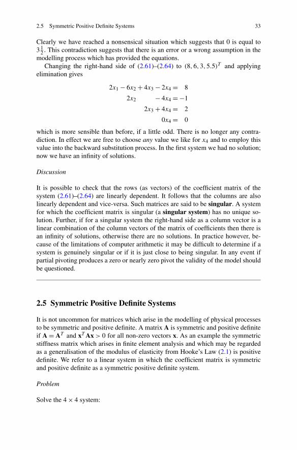
Changing the right-hand side of (2.61)–(2.64) to (8,6,3,5.5)T and applyingelimination gives
2x1 − 6x2 + 4x3 − 2x4 = 8
2x2 − 4x4 = −1
2x3 + 4x4 = 2
0x4 = 0
which is more sensible than before, if a little odd. There is no longer any contra-diction. In effect we are free to choose any value we like for x4 and to employ thisvalue into the backward substitution process. In the first system we had no solution;now we have an infinity of solutions.
Discussion
It is possible to check that the rows (as vectors) of the coefficient matrix of thesystem (2.61)–(2.64) are linearly dependent. It follows that the columns are alsolinearly dependent and vice-versa. Such matrices are said to be singular. A systemfor which the coefficient matrix is singular (a singular system) has no unique so-lution. Further, if for a singular system the right-hand side as a column vector is alinear combination of the column vectors of the matrix of coefficients then there isan infinity of solutions, otherwise there are no solutions. In practice however, be-cause of the limitations of computer arithmetic it may be difficult to determine if asystem is genuinely singular or if it is just close to being singular. In any event ifpartial pivoting produces a zero or nearly zero pivot the validity of the model shouldbe questioned.
2.5 Symmetric Positive Definite Systems
It is not uncommon for matrices which arise in the modelling of physical processesto be symmetric and positive definite. A matrix A is symmetric and positive definiteif A = AT and xT Ax > 0 for all non-zero vectors x. As an example the symmetricstiffness matrix which arises in finite element analysis and which may be regardedas a generalisation of the modulus of elasticity from Hooke’s Law (2.1) is positivedefinite. We refer to a linear system in which the coefficient matrix is symmetricand positive definite as a symmetric positive definite system.
Problem
Solve the 4 × 4 system:
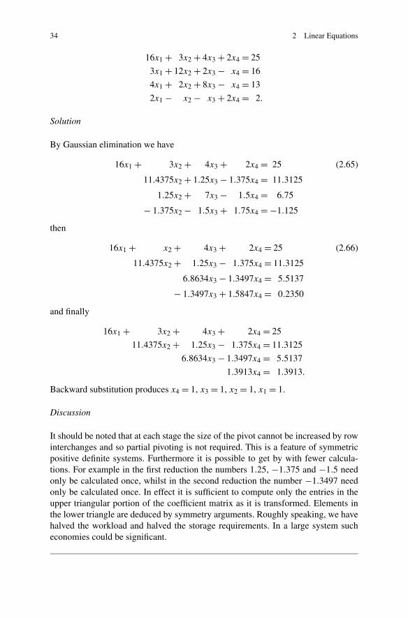
34 2 Linear Equations
16x1 + 3x2 + 4x3 + 2x4 = 25
3x1 + 12x2 + 2x3 − x4 = 16
4x1 + 2x2 + 8x3 − x4 = 13
2x1 − x2 − x3 + 2x4 = 2.
Solution
By Gaussian elimination we have
16x1 + 3x2 + 4x3 + 2x4 = 25 (2.65)
11.4375x2 + 1.25x3 − 1.375x4 = 11.3125
1.25x2 + 7x3 − 1.5x4 = 6.75
− 1.375x2 − 1.5x3 + 1.75x4 = −1.125
then
16x1 + x2 + 4x3 + 2x4 = 25 (2.66)
11.4375x2 + 1.25x3 − 1.375x4 = 11.3125
6.8634x3 − 1.3497x4 = 5.5137
− 1.3497x3 + 1.5847x4 = 0.2350
and finally
16x1 + 3x2 + 4x3 + 2x4 = 25
11.4375x2 + 1.25x3 − 1.375x4 = 11.3125
6.8634x3 − 1.3497x4 = 5.5137
1.3913x4 = 1.3913.
Backward substitution produces x4 = 1, x3 = 1, x2 = 1, x1 = 1.
Discussion
It should be noted that at each stage the size of the pivot cannot be increased by rowinterchanges and so partial pivoting is not required. This is a feature of symmetricpositive definite systems. Furthermore it is possible to get by with fewer calcula-tions. For example in the first reduction the numbers 1.25, −1.375 and −1.5 needonly be calculated once, whilst in the second reduction the number −1.3497 needonly be calculated once. In effect it is sufficient to compute only the entries in theupper triangular portion of the coefficient matrix as it is transformed. Elements inthe lower triangle are deduced by symmetry arguments. Roughly speaking, we havehalved the workload and halved the storage requirements. In a large system sucheconomies could be significant.
2.6 Iterative Refinement 35
Although it is easy to test the symmetry of a given matrix, it is not so easy to es-tablish if a symmetric matrix is positive definite. A symmetric matrix is positivedefinite if it diagonally dominant (that is if each diagonal element is larger in ab-solute value than the sum of the absolute values of the other elements on the samerow). However being diagonally dominant is not a necessary condition for a sym-metric matrix to be positive definite. Often the only real way to check is to applyGaussian elimination. If, at any stage, partial pivoting is necessary then the matrix isnot positive definite. In practice therefore when the modelling process requires therepeated solution of a symmetric linear system it is advisable to try the system ona program which assumes that the coefficient matrix is positive definite, but whichflags an error if a non-positive definite condition is detected.
2.6 Iterative Refinement
The effect of rounding error in Gaussian elimination is to yield a computed solutionwhich is a perturbation of the mathematically correct solution. Partial pivoting mayhelp to reduce the accumulative effect of these errors, but there is no guaranteethat it will eliminate them entirely. Iterative refinement is a process by which a firstcomputed solution can sometimes be improved to yield a more accurate solution. Inthe following example we illustrate the method by working to limited accuracy anddrawing conclusions that may be applied when using computer arithmetic.
Problem
Solve the 4 × 4 system
0.366x1 + 0.668x2 − 0.731x3 − 0.878x4 = −0.575 (2.67)
0.520x1 + 0.134x2 − 0.330x3 + 0.484x4 = 0.808 (2.68)
0.738x1 − 0.826x2 + 0.194x3 − 0.204x4 = −0.098 (2.69)
0.382x1 − 0.667x2 + 0.270x3 − 0.255x4 = −0.270 (2.70)
using Gaussian elimination.
Solution
The system has the exact solution x1 = 1, x2 = 1, x3 = 1 and x4 = 1. However,working to just three significant figures, Gaussian elimination with partial pivotingproduces a solution x1 = 1.14, x2 = 1.18, x3 = 1.23 and x4 = 0.993. Substitutingthese values back into the left-hand side of the equations and working to three-figureaccuracy produces −0.575, 0.808, −0.0908 and −0.270, which suggests that thiscomputed solution is accurate. However repeating the substitution and working tosix significant figures produces a slightly different set of values. Subtracting thethree-figure result from the corresponding six-figure result for each equation, gives
36 2 Linear Equations
differences of −0.00950 for (2.67), −0.0176 for (2.68), −0.000688 for (2.69) and0.00269 for (2.70). These differences are known as residuals. Since these residualvalues are small in relation to the coefficients in the equation we can suppose we arefairly close to the true solution.
More formally, if we were to assume that the true solution differs from our cal-culated 3-figure solution by amounts δ1, δ2, δ3 and δ4, that is the true solution is1.14 + δx1, 1.18 + δ2, 1.23 + δ3, 0.993 + δx4, we would have
0.366(1.14 + δ1) + 0.668(1.18 + δ2)
−0.731(1.23 + δ3) − 0.878(0.993 + δ4) = −0.575
0.520(1.14 + δ1) + 0.134(1.18 + δ2)
−0.330(1.23 + δ3) + 0.484(0.993 + δ4) = 0.808
0.738(1.14 + δ1) − 0.826(1.18 + δ2)
+0.194(1.23 + δ3) − 0.204(0.993 + δ4) = −0.098
0.382(1.14 + δ1) − 0.667(1.18 + δ2)
+0.270(1.23 + δ3) − 0.255(0.993 + δ4) = −0.270.
We are now in a position to find the corrections δ1, δ2, δ3 and δ4. Using the calcula-tions we have already performed to find the residuals we have
0.366δ1 + 0.668δ2 − 0.731δ3 − 0.878δ4 = −0.00950
0.520δ1 + 0.134δ2 − 0.330δ3 + 0.484δ4 = −0.0176
0.738δ1 − 0.826δ2 + 0.194δ3 − 0.204δ4 = −0.000688
0.382δ1 − 0.667δ2 + 0.270δ3 − 0.255δ4 = 0.00269.
Using 3 significant figure arithmetic again we find that Gaussian elimination withpartial pivoting produces a solution δ1 = −0.130, δ2 = −0.166, δ3 = −0.210 andδ4 = 0.00525, and adding these values to our initial solution gives x1 = 1.01, x2 =1.01, x3 = 1.02 and x4 = 0.998. Although this is still not completely accurate, it isslightly better than the previous solution.
Discussion
The example is an illustration of the technique known as iterative refinement. Com-puter calculations inevitably involve rounding errors which result from performingarithmetic to a limited accuracy. Iterative refinement is used to try to restore a littlemore accuracy to an existing solution. However it does depend upon being able tocalculate the residuals with some accuracy and this will involve using arithmeticwhich is more accurate than that of the rest of the calculations. Note that the orig-inal coefficient matrix is used in finding the improved solution and this can leadto economies when applied to large systems. The method of iterative refinement asused with Gaussian elimination is summarised in Table 2.3.
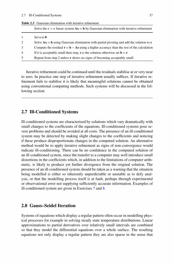
2.7 Ill-Conditioned Systems 37
Table 2.3 Gaussian elimination with iterative refinement
Solve the n × n linear system Ax = b by Gaussian elimination with iterative refinement
1 Set s to 0
2 Solve Ax = b using Gaussian elimination with partial pivoting and add the solution to s
3 Compute the residual r = b − As using a higher accuracy than the rest of the calculation
4 If r is acceptably small then stop, s is the solution otherwise set b = r
5 Repeat from step 2 unless r shows no signs of becoming acceptably small
Iterative refinement could be continued until the residuals stabilise at or very nearto zero. In practice one step of iterative refinement usually suffices. If iterative re-finement fails to stabilise it is likely that meaningful solutions cannot be obtainedusing conventional computing methods. Such systems will be discussed in the fol-lowing section.
2.7 Ill-Conditioned Systems
Ill-conditioned systems are characterised by solutions which vary dramatically withsmall changes to the coefficients of the equations. Ill-conditioned systems pose se-vere problems and should be avoided at all costs. The presence of an ill-conditionedsystem may be detected by making slight changes to the coefficients and noticingif these produce disproportionate changes in the computed solution. An alternativemethod would be to apply iterative refinement as signs of non-convergence wouldindicate ill-conditioning. There can be no confidence in the computed solution ofan ill-conditioned system, since the transfer to a computer may well introduce smalldistortions in the coefficients which, in addition to the limitations of computer arith-metic, is likely to produce yet further divergence from the original solution. Thepresence of an ill-conditioned system should be taken as a warning that the situationbeing modelled is either so inherently unpredictable or unstable as to defy anal-ysis, or that the modelling process itself is at fault, perhaps through experimentalor observational error not supplying sufficiently accurate information. Examples ofill-conditioned system are given in Exercises 7 and 8.
2.8 Gauss–Seidel Iteration
Systems of equations which display a regular pattern often occur in modelling phys-ical processes for example in solving steady state temperature distributions. Linearapproximations to partial derivatives over relatively small intervals are combinedso that they model the differential equations over a whole surface. The resultingequations not only display a regular pattern they are also sparse in the sense that
38 2 Linear Equations
although the number of equations may be large, possibly hundreds or thousands,the number of variables in each equation is very much smaller, reflecting the way inwhich they have been assembled over small areas. It is perfectly possible to solvesuch systems using the elimination techniques considered earlier in this chapter, butthat may cause storage and indexing problems. It would be possible to store a sparsecoefficient matrix in a condensed form by just recording and indexing non-zero el-ements but the sparse quality would probably be quickly destroyed by Gaussianelimination. We consider an alternative, iterative approach to solving large sparsesystems.
Problem
Solve the following system of equations using Gauss–Seidel iteration.
6x1 + x2 = 1
x1 + 6x2 + x3 = 1
x2 + 6x3 + x4 = 1. . .
x8 + 6x9 + x10 = 1
x9 + 6x10 = 1.
Solution
We adopt an iterative approach to obtaining a solution. We start with an initial guessat the solution and then form a series of further approximations which we hopeeventually leads to a solution. We start by writing the equations as
x1 = 1 − x2
6(2.71)
x2 = 1 − x1 − x3
6(2.72)
... (2.73)
x9 = 1 − x7 − x8
6(2.74)
x10 = 1 − x9
6. (2.75)
As an initial guess at the solution we set each of x1, x2, . . . , x10 to 16 , not an unrea-
sonable choice since this is the solution if we ignore the off-diagonal terms in theoriginal coefficient matrix.
We have from (2.71)
x1 = 1 − 16
6= 0.1389
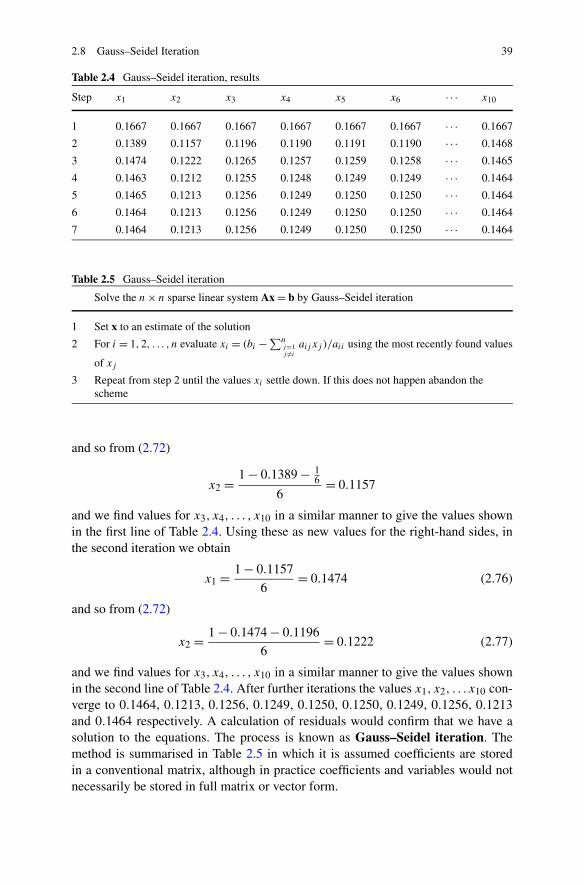
2.8 Gauss–Seidel Iteration 39
Table 2.4 Gauss–Seidel iteration, results
Step x1 x2 x3 x4 x5 x6 · · · x10
1 0.1667 0.1667 0.1667 0.1667 0.1667 0.1667 · · · 0.1667
2 0.1389 0.1157 0.1196 0.1190 0.1191 0.1190 · · · 0.1468
3 0.1474 0.1222 0.1265 0.1257 0.1259 0.1258 · · · 0.1465
4 0.1463 0.1212 0.1255 0.1248 0.1249 0.1249 · · · 0.1464
5 0.1465 0.1213 0.1256 0.1249 0.1250 0.1250 · · · 0.1464
6 0.1464 0.1213 0.1256 0.1249 0.1250 0.1250 · · · 0.1464
7 0.1464 0.1213 0.1256 0.1249 0.1250 0.1250 · · · 0.1464
Table 2.5 Gauss–Seidel iteration
Solve the n × n sparse linear system Ax = b by Gauss–Seidel iteration
1 Set x to an estimate of the solution
2 For i = 1,2, . . . , n evaluate xi = (bi − ∑nj=1j �=i
aij xj )/aii using the most recently found values
of xj
3 Repeat from step 2 until the values xi settle down. If this does not happen abandon thescheme
and so from (2.72)
x2 = 1 − 0.1389 − 16
6= 0.1157
and we find values for x3, x4, . . . , x10 in a similar manner to give the values shownin the first line of Table 2.4. Using these as new values for the right-hand sides, inthe second iteration we obtain
x1 = 1 − 0.1157
6= 0.1474 (2.76)
and so from (2.72)
x2 = 1 − 0.1474 − 0.1196
6= 0.1222 (2.77)
and we find values for x3, x4, . . . , x10 in a similar manner to give the values shownin the second line of Table 2.4. After further iterations the values x1, x2, . . . x10 con-verge to 0.1464, 0.1213, 0.1256, 0.1249, 0.1250, 0.1250, 0.1249, 0.1256, 0.1213and 0.1464 respectively. A calculation of residuals would confirm that we have asolution to the equations. The process is known as Gauss–Seidel iteration. Themethod is summarised in Table 2.5 in which it is assumed coefficients are storedin a conventional matrix, although in practice coefficients and variables would notnecessarily be stored in full matrix or vector form.
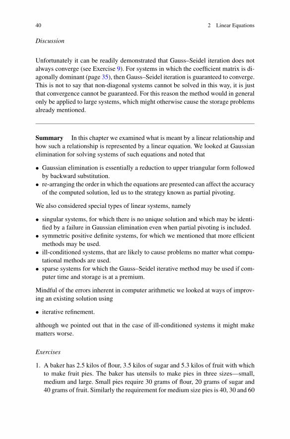
40 2 Linear Equations
Discussion
Unfortunately it can be readily demonstrated that Gauss–Seidel iteration does notalways converge (see Exercise 9). For systems in which the coefficient matrix is di-agonally dominant (page 35), then Gauss–Seidel iteration is guaranteed to converge.This is not to say that non-diagonal systems cannot be solved in this way, it is justthat convergence cannot be guaranteed. For this reason the method would in generalonly be applied to large systems, which might otherwise cause the storage problemsalready mentioned.
Summary In this chapter we examined what is meant by a linear relationship andhow such a relationship is represented by a linear equation. We looked at Gaussianelimination for solving systems of such equations and noted that
• Gaussian elimination is essentially a reduction to upper triangular form followedby backward substitution.
• re-arranging the order in which the equations are presented can affect the accuracyof the computed solution, led us to the strategy known as partial pivoting.
We also considered special types of linear systems, namely
• singular systems, for which there is no unique solution and which may be identi-fied by a failure in Gaussian elimination even when partial pivoting is included.
• symmetric positive definite systems, for which we mentioned that more efficientmethods may be used.
• ill-conditioned systems, that are likely to cause problems no matter what compu-tational methods are used.
• sparse systems for which the Gauss–Seidel iterative method may be used if com-puter time and storage is at a premium.
Mindful of the errors inherent in computer arithmetic we looked at ways of improv-ing an existing solution using
• iterative refinement.
although we pointed out that in the case of ill-conditioned systems it might makematters worse.
Exercises
1. A baker has 2.5 kilos of flour, 3.5 kilos of sugar and 5.3 kilos of fruit with whichto make fruit pies. The baker has utensils to make pies in three sizes—small,medium and large. Small pies require 30 grams of flour, 20 grams of sugar and40 grams of fruit. Similarly the requirement for medium size pies is 40, 30 and 60

2.8 Gauss–Seidel Iteration 41
grams respectively, and for large pies 60, 50 and 90 grams. The baker wishes touse up all the ingredients. Formulate a linear system to decide if this is possible.
Let the number of small, medium and large pies to be made be x, y and z.Taking into account that 1 kilo = 1000 grams we have
3x + 2y + 4z = 250 (flour to be used)
4x + 3y + 6z = 350 (sugar to be used)
6x + 5y + 9z = 530 (fruit to be used).
If the solution to these equations turns out to consist of whole numbers then thebaker can use up all the ingredients. If some or all of x, y and z were not wholenumbers then the baker is not able to use up all the ingredients, deciding howmany pies of each size to make in order to minimise the quantity of ingredientsleft over is the type of problem we look at in Chap. 7.
Assuming the equations are written in the form Ax = b use the followingcode to find a solution. The code uses the left-division operator, \ as describedin Sect. 1.4.
A = [ 3 2 4; 4 3 6; 6 5 9 ]b = [ 250 350 530 ] 'x = A\b
2. (i) Reduce the following linear system to upper triangular form.
2x1 − x2 − 4x3 = 5
x1 + x2 + 2x3 = 0
6x1 + 3x2 − x3 = −2.5.
Form the matrix of coefficients of the upper triangular system in the matrix Uand the corresponding right-side in the vector r. Use the following Matlab codeto make copies of A and b in U and r respectively. A multiple (the pivot) of row 1is subtracted from row 2 and row 3, then a multiple (another pivot) of row 2 issubtracted from row 3.
U = A;r = b;for row = 1 : 2;
for i = row + 1 : 3;pivot=U(i, row)/U(row, row)U(i, :) = U (i, :) − pivot * U(row, :)r(i) = r(i) − pivot∗ r(row)
endend
As something of a programming challenge try modifying the code to handlelarger matrices and to allow partial pivoting and deal with zero pivots.
(ii) Take the solution from part (i) and apply backward substitution to finda solution to the original linear system. Use the following Matlab code, which
42 2 Linear Equations
assumes that the coefficients of the upper triangular system are stored in thematrix U and that the modified right hands are stored in r.
x(3) = r(3)/U(3, 3);for i = 2 : −1 : 1
sum = 0;for j = i+1 : 3 ;
sum = sum + U(i, j)*x(j);end;x(i) = (r(i) − sum)/U (i, i);
end;x
Check the validity of the solution by evaluating U ∗ x, where x is the solution asa column vector. All being well this should produce the original b.
3. Matlab has a function lu which provides the LU factorisation of a matrix. Formthe matrix, A of coefficients of the following system in a Matlab program.
x1 + 2x2 + 3x3 + x4 = 8
2x1 + 4x2 − x3 + x4 = 1
x1 + 3x2 − x3 + 2x4 = 1
−3x1 − x2 − 3x3 + 2x4 = −7.
Use the lu command in the form [L U] =lu(A), which returns an upper triangularU and a (possibly) permuted lower triangular L so that Ax = LUb, where b isthe column vector of right-sides.
Having established matrices L and U we have LUx = b. Writing Ly = b, findy by using the left-division operator. We now have Ux = y. Find x by using theleft-division operator. Check the result by comparing Ax and b.
Alternatively use the lu command in the form [L U P] = lu(A) so that U isnot permuted and a permutation matrix P is returned. In this case b would bereplaced by Pb in the scheme shown above, and so x could be found by left-division.
4. As an example of how rounding error can affect the solutions to even relativelysmall systems solve the following equations using the Matlab left-division \ op-erator.
−0.6210x1 0.0956x2 −0.0445x3 0.8747x4 = 5.3814
0.4328x1 −0.0624x2 8.8101x3 −1.0393x4 = −1.0393
−0.0004x1 −0.0621x2 5.3852x3 −0.3897x4 = −0.3897
3.6066x1 0.6536x2 0.8460x3 −0.2000x4 = −0.0005
Use both 64-bit precision (the default option) and then use 32-bit precision byconverting the variables using the single operator, for example B = single(A).For both cases set format long to show the maximum number of decimal placesfor the chosen word length.
2.8 Gauss–Seidel Iteration 43
5. Form an LU factorisation of the following symmetric matrix to show that it isnot positive definite. ⎛
⎜⎜⎝4 1 −1 21 3 −2 −1
−1 −2 1 62 −1 6 1
⎞⎟⎟⎠
Using a little ingenuity we can find a non-zero vector such as xT = (0 1 1 0)
that does not satisfy the requirement xT Ax > 0.6. Show that the following system has no solution.
2x1 + 3x2 + 4x3 = 2
x1 − 2x2 + 3x3 = 5
3x1 + x2 + 7x3 = 8
Use the LU factorisation as provided by the function lu to show that the matrix ofcoefficients is singular. Show by algebraic manipulation that the system does nothave a unique solution. Decide if there is no solution or an infinity of solutions.
7. Solve the following systems of linear equations, one of which is a slight variationof the other to show that we have a example of an ill-conditioning
0.9740x1 0.7900x2 0.3110x3 = 1.0
−0.6310x1 0.4700x2 0.2510x3 = 0.5
0.4550x1 0.9750x2 0.4250x3 = 0.75
0.9736x1 0.7900x2 0.3110x3 = 1.0
−0.6310x1 0.4700x2 0.2506x3 = 0.5
0.4550x1 0.9746x2 0.4250x3 = 0.75.
8. As an example of severe ill-conditioning consider the Hilbert2 matrix Hn, whichhas the form
Hn =
⎛⎜⎜⎜⎜⎜⎜⎜⎝
1 1/2 1/3 1/4 . . . 1/n
1/2 1/3 1/4 1/5 . . . 1/(n + 1)
1/3 1/4 1/5 1/6 . . .
1/4 1/5 1/6 1/7 . . ....
...
1/n 1/(n + 1) . . . 1/(2n − 1)
⎞⎟⎟⎟⎟⎟⎟⎟⎠
.
Use the Matlab command x = ones(n,1) to generate a column vector x of n
1’s and the command H = hilb(n) to generate the Hilbert matrix Hn of order n.Form the vector bn = Hnx.
Solve the system Hnx = bn for various n using the left division operator. Intheory x should be (1, . . . ,1), but see what happens. Begin with n = 3 increasethe value with suitable increments up to around n = 18 to show the effects ofill-conditioning and rounding error. Iterative refinement will not be of any helpin this case.
2David Hilbert, 1862–1943. In 1900 he put forward a list of 23 important unsolved problems someof which remain unsolved.
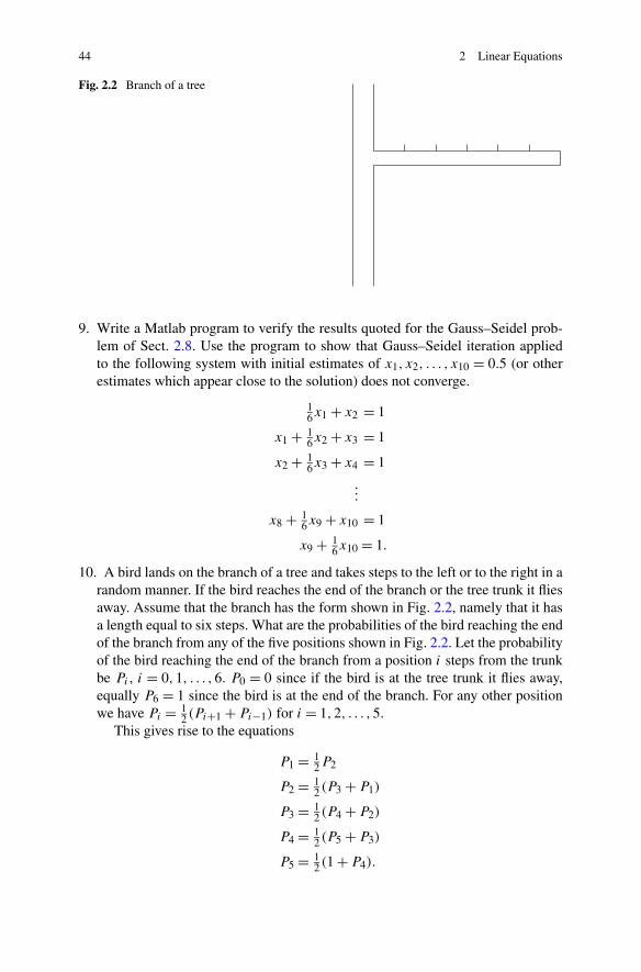
44 2 Linear Equations
Fig. 2.2 Branch of a tree
9. Write a Matlab program to verify the results quoted for the Gauss–Seidel prob-lem of Sect. 2.8. Use the program to show that Gauss–Seidel iteration appliedto the following system with initial estimates of x1, x2, . . . , x10 = 0.5 (or otherestimates which appear close to the solution) does not converge.
16x1 + x2 = 1
x1 + 16x2 + x3 = 1
x2 + 16x3 + x4 = 1
...
x8 + 16x9 + x10 = 1
x9 + 16x10 = 1.
10. A bird lands on the branch of a tree and takes steps to the left or to the right in arandom manner. If the bird reaches the end of the branch or the tree trunk it fliesaway. Assume that the branch has the form shown in Fig. 2.2, namely that it hasa length equal to six steps. What are the probabilities of the bird reaching the endof the branch from any of the five positions shown in Fig. 2.2. Let the probabilityof the bird reaching the end of the branch from a position i steps from the trunkbe Pi , i = 0,1, . . . ,6. P0 = 0 since if the bird is at the tree trunk it flies away,equally P6 = 1 since the bird is at the end of the branch. For any other positionwe have Pi = 1
2 (Pi+1 + Pi−1) for i = 1,2, . . . ,5.This gives rise to the equations
P1 = 12P2
P2 = 12 (P3 + P1)
P3 = 12 (P4 + P2)
P4 = 12 (P5 + P3)
P5 = 12 (1 + P4).

2.8 Gauss–Seidel Iteration 45
Set up a Gauss–Seidel iterative scheme in Matlab to solve the problem. Chooseinitial estimates such as Pi = 0, i = 1,2, . . . ,5. Confirm that the results are inline with expectations.
Chapter 3Nonlinear Equations
Aims In this chapter we look at a variety of methods that can be used to find a root(or zero, the terms are interchangeable) of a function f (x) or a single variable x,which is equivalent to solving the equation f (x) = 0. We will also look at a methodfor solving systems of nonlinear equations and so we extend the scope of Chap. 2which only considered systems of linear equations.
We look at the following root-finding methods for a single nonlinear equation
• the bisection method.• false position.• the secant method.• the Newton–Raphson1 method.• Newton’s method for a system of nonlinear equations.
It should be noted that in general a nonlinear equation will have a number of roots;for example, if f is polynomial of degree n in x then it has n roots, some of whichmay be multiple roots. Further, some, or all, of the roots of a polynomial equationmay be complex. The methods we investigate are designed to locate an individualreal root of a function f (x) within a given range of x values.
Overview The problems involved in finding a root of an equation which models anonlinear relationship are more complex than those for linear equations. Indeed it isnot possible to provide a method which can be guaranteed to work for every singlecase. For this reason it is as well to be acquainted with more than one method and tobe aware of the strengths and weaknesses of particular methods through theoreticalinsight and practical experience. The four methods for a single nonlinear equationare all of the same basic, iterative, form. Starting with one or more approximationsto a root of the equation f (x) = 0 they generate a sequence that may or may notconverge to a root. The differences lie in
1Joseph Raphson, 1648–1715, English mathematician credited with the independent discovery ofNewton’s method for solving equations numerically.
C. Woodford, C. Phillips, Numerical Methods with Worked Examples: Matlab Edition,DOI 10.1007/978-94-007-1366-6_3, © Springer Science+Business Media B.V. 2012
47
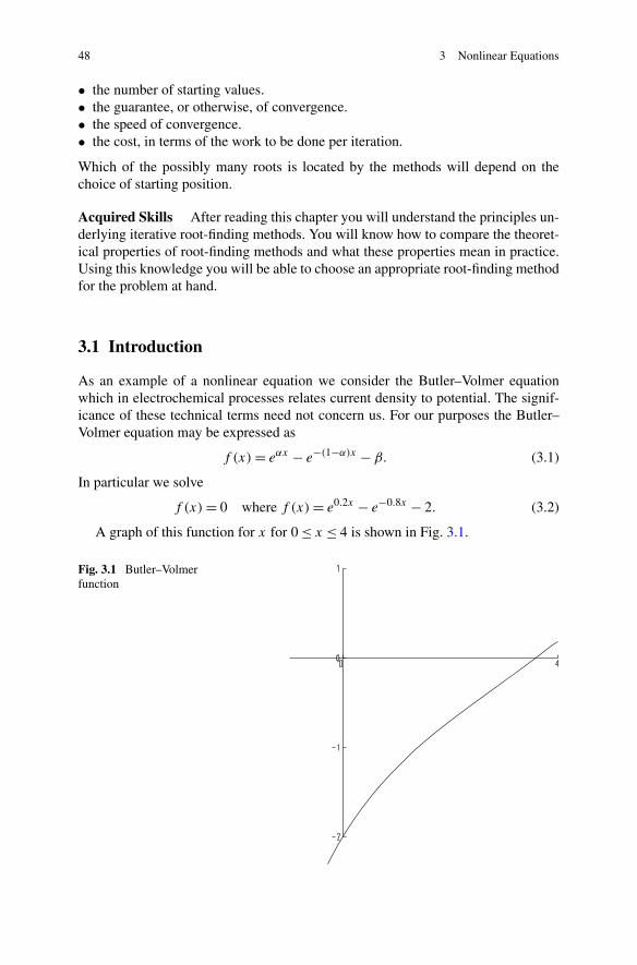
48 3 Nonlinear Equations
• the number of starting values.• the guarantee, or otherwise, of convergence.• the speed of convergence.• the cost, in terms of the work to be done per iteration.
Which of the possibly many roots is located by the methods will depend on thechoice of starting position.
Acquired Skills After reading this chapter you will understand the principles un-derlying iterative root-finding methods. You will know how to compare the theoret-ical properties of root-finding methods and what these properties mean in practice.Using this knowledge you will be able to choose an appropriate root-finding methodfor the problem at hand.
3.1 Introduction
As an example of a nonlinear equation we consider the Butler–Volmer equationwhich in electrochemical processes relates current density to potential. The signif-icance of these technical terms need not concern us. For our purposes the Butler–Volmer equation may be expressed as
f (x) = eαx − e−(1−α)x − β. (3.1)
In particular we solve
f (x) = 0 where f (x) = e0.2x − e−0.8x − 2. (3.2)
A graph of this function for x for 0 ≤ x ≤ 4 is shown in Fig. 3.1.
Fig. 3.1 Butler–Volmerfunction

3.2 Bisection Method 49
3.2 Bisection Method
The bisection method is the simplest of all the methods for finding a root of a non-linear equation. We start with an interval containing a root and divide it into a leftand a right half. We decide which of the two halves contains a root and proceed witha further division of that half. We do this repeatedly until the interval containing aroot is sufficiently narrowed down to meet the level of accuracy required. If we takethe mid-point of the latest interval to be an approximation to a root, we can say thatthis is accurate to within ± half the width of the interval.
Problem
Use the method of bisection to find a root of the equation
f (x) = 0 where f (x) = e0.2x − e−0.8x − 2.
Solution
From Fig. 3.1 we know that there is a single root of the equation in the interval[0,4]. f (0) is negative and f (4) is positive, and since the function is continuous,as x increases from 0 to 4 at some point f must cross over from being negative topositive and have the value 0.
At the mid-point of the interval, where x = 2, we find that f (2) = −0.71007. Itfollows that there must be a root of the function to the right of x = 2 since f (2) isnegative and f (4) is positive. That is, having started with the interval [0,4] we nowknow that there is a root of the function in the reduced interval [2,4].
We now look at [2,4] for which the mid-point is x = 3. Since f (3) is −0.26860,which is negative, we know there must be a root of the function in the further re-duced interval [3,4]. Continuing in a similar manner we produce the sequence ofintervals shown in Table 3.1, each of which is known to contain a root of the equa-tion.
Table 3.1 Sequence ofintervals obtained bybisection
a b a+b2 f (a) f ( a+b
2 ) f (b)
0 4 2 −2 −0.71007 0.18478
2 4 3 −0.71007 −0.26860 0.18478
3 4 3.5 −0.26860 −0.04706 0.18478
3.5 4 3.75 −0.04706 0.06721 0.18478
3.5 3.75 3.625 −0.04706 0.00971 0.06721
3.5 3.75 3.625 −0.04706 0.00971 0.06721
3.5 3.625 3.5625 −0.04706 −0.01876 0.00971
3.5625 3.5625 3.59375 −0.01876 −0.00455 0.00971
3.59375 3.625 3.60938 −0.00455 0.00257 0.00971
50 3 Nonlinear Equations
Table 3.2 The bisectionmethod Solve f (x) = 0 by bisection
1 Find an interval [a, b] in which f (x) = 0
2 Set x∗ to a+b2
3 Calculate f (x∗)4 Test for convergence
5 If f (x∗) and f (b) have opposite sign set a to x∗, otherwiseset b to x∗
6 Repeat from step 2
Discussion
We have to decide when to stop the procedure and this will depend upon the problemunder consideration. In terms of absolute values we can deduce from Table 3.1 thatwe have a range of x values [3.59375,3.60938] for which f is to within ±0.005of zero. It is important to distinguish between absolute error, which we have justdescribed and relative error which measures relative values. In this example therelative values might be measured as the ratios a−b
aand f (a)−f (b)
f (a). In practice the
level of acceptable error would be decided in advance.Furthermore in considering finding a root of a function f (x) we have to take
into account a possible imbalance between x and f (x) values. If for example thefunction has a very steep slope at the root, the range of x values producing a functionvalues close to zero could be of a much smaller order of magnitude. Conversely, ifthe function is very flat in the region of a root the range of possible x values wouldbe comparatively large. The bisection method allowing for a choice of absolute orrelative error checking and criteria based on either x and/or f (x) values as the testfor convergence is summarised in Table 3.2.
3.2.1 Finding an Interval Containing a Root
In the case of the function already considered we were fortunate to have available agraph which could be used to determine an initial interval containing a root. How-ever if such a graph is not readily available it would be advisable to generate a seriesof x and f values to gain a feel for the function and the presence of roots and en-closing intervals. In the event of a function having multiple roots care should betaken to choose an interval containing just one root, otherwise the bisection method(and the other methods to be considered) may yield a value which is inappropriateto the problem being modelled.
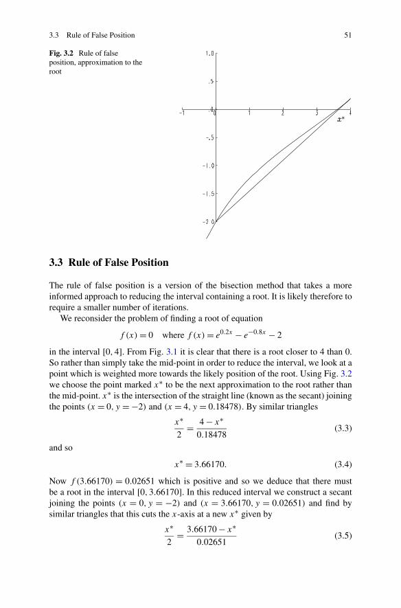
3.3 Rule of False Position 51
Fig. 3.2 Rule of falseposition, approximation to theroot
3.3 Rule of False Position
The rule of false position is a version of the bisection method that takes a moreinformed approach to reducing the interval containing a root. It is likely therefore torequire a smaller number of iterations.
We reconsider the problem of finding a root of equation
f (x) = 0 where f (x) = e0.2x − e−0.8x − 2
in the interval [0,4]. From Fig. 3.1 it is clear that there is a root closer to 4 than 0.So rather than simply take the mid-point in order to reduce the interval, we look at apoint which is weighted more towards the likely position of the root. Using Fig. 3.2we choose the point marked x∗ to be the next approximation to the root rather thanthe mid-point. x∗ is the intersection of the straight line (known as the secant) joiningthe points (x = 0, y = −2) and (x = 4, y = 0.18478). By similar triangles
x∗
2= 4 − x∗
0.18478(3.3)
and so
x∗ = 3.66170. (3.4)
Now f (3.66170) = 0.02651 which is positive and so we deduce that there mustbe a root in the interval [0,3.66170]. In this reduced interval we construct a secantjoining the points (x = 0, y = −2) and (x = 3.66170, y = 0.02651) and find bysimilar triangles that this cuts the x-axis at a new x∗ given by
x∗
2= 3.66170 − x∗
0.02651(3.5)
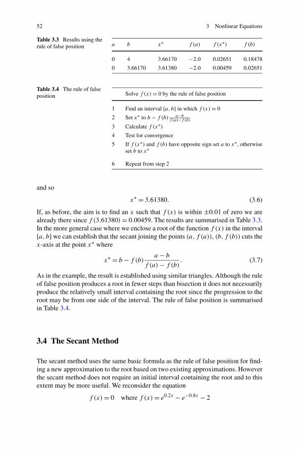
52 3 Nonlinear Equations
Table 3.3 Results using therule of false position a b x∗ f (a) f (x∗) f (b)
0 4 3.66170 −2.0 0.02651 0.18478
0 3.66170 3.61380 −2.0 0.00459 0.02651
Table 3.4 The rule of falseposition Solve f (x) = 0 by the rule of false position
1 Find an interval [a, b] in which f (x) = 0
2 Set x∗ to b − f (b) a−bf (a)−f (b)
3 Calculate f (x∗)4 Test for convergence
5 If f (x∗) and f (b) have opposite sign set a to x∗, otherwiseset b to x∗
6 Repeat from step 2
and so
x∗ = 3.61380. (3.6)
If, as before, the aim is to find an x such that f (x) is within ±0.01 of zero we arealready there since f (3.61380) = 0.00459. The results are summarised in Table 3.3.In the more general case where we enclose a root of the function f (x) in the interval[a, b] we can establish that the secant joining the points (a, f (a)), (b, f (b)) cuts thex-axis at the point x∗ where
x∗ = b − f (b)a − b
f (a) − f (b). (3.7)
As in the example, the result is established using similar triangles. Although the ruleof false position produces a root in fewer steps than bisection it does not necessarilyproduce the relatively small interval containing the root since the progression to theroot may be from one side of the interval. The rule of false position is summarisedin Table 3.4.
3.4 The Secant Method
The secant method uses the same basic formula as the rule of false position for find-ing a new approximation to the root based on two existing approximations. Howeverthe secant method does not require an initial interval containing the root and to thisextent may be more useful. We reconsider the equation
f (x) = 0 where f (x) = e0.2x − e−0.8x − 2

3.4 The Secant Method 53
Fig. 3.3 Secant method,approximation to the root
to illustrate the method by choosing two arbitrary values from which to proceed.For no particular reason we choose x = 5 as the first point and x = 4 as the secondpoint. We note that initial function values need not be of opposite sign. We havef (5) = 0.69997 and f (4) = 0.18478. On the basis of Fig. 3.3 the point marked x∗is likely to be a better approximation to the root.
By similar triangles we have
4 − x∗
0.18478= 5 − x∗
0.69997(3.8)
and so
x∗ = 3.64134. (3.9)
Now f (3.64134) = 0.01718 and so we are getting closer to the root. We repeat themethod by discarding the oldest estimate (in this case, x = 5) and retaining the twolatest estimates (x = 4 and x = 3.64134) and then find another, x∗ given by
3.64134 − x∗
0.01718= 4 − x∗
0.18478(3.10)
and so
x∗ = 3.60457. (3.11)
If, as before, the aim is to find an x such that f (x) is within ±0.01 of root we arealready there since f (3.60457) = 0.00038. To carry the method one stage further wediscard x = 4 and retain x = 3.64134 and x = 3.60457. The next estimate is x∗ =3.60373 for which f (3.60373) = 0.0 (to 6 decimal places). The sequence is shownin Table 3.5. On the evidence presented here, the secant method converges to a rootmore quickly than either bisection or the rule of false position. Moreover initialestimates that are wildly inaccurate may still provide a root. A typical progression
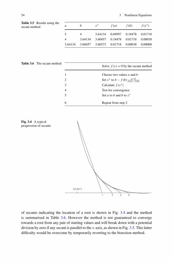
54 3 Nonlinear Equations
Table 3.5 Results using thesecant method a b x∗ f (a) f (b) f (x∗)
5 4 3.64134 0.69997 0.18478 0.01718
4 3.64134 3.60457 0.18478 0.01718 0.00038
3.64134 3.60457 3.60373 0.01718 0.00038 0.00000
Table 3.6 The secant methodSolve f (x) = 0 by the secant method
1 Choose two values a and b
2 Set x∗ to b − f (b) a−bf (a)−f (b)
3 Calculate f (x∗)4 Test for convergence
5 Set a to b and b to x∗
6 Repeat from step 2
Fig. 3.4 A typicalprogression of secants
of secants indicating the location of a root is shown in Fig. 3.4 and the methodis summarised in Table 3.6. However the method is not guaranteed to convergetowards a root from any pair of starting values and will break down with a potentialdivision by zero if any secant is parallel to the x-axis, as shown in Fig. 3.5. This latterdifficulty would be overcome by temporarily reverting to the bisection method.
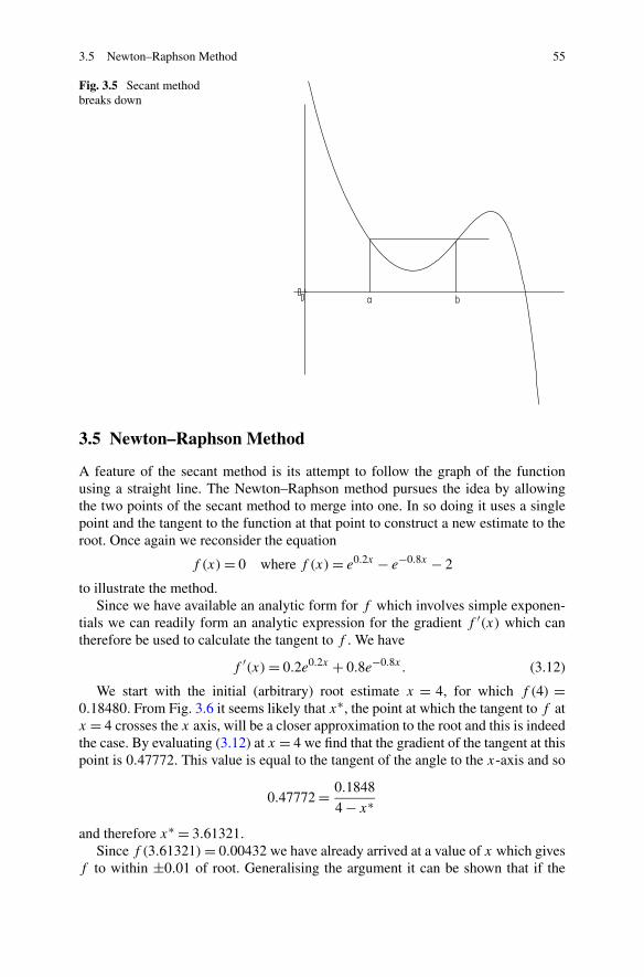
3.5 Newton–Raphson Method 55
Fig. 3.5 Secant methodbreaks down
3.5 Newton–Raphson Method
A feature of the secant method is its attempt to follow the graph of the functionusing a straight line. The Newton–Raphson method pursues the idea by allowingthe two points of the secant method to merge into one. In so doing it uses a singlepoint and the tangent to the function at that point to construct a new estimate to theroot. Once again we reconsider the equation
f (x) = 0 where f (x) = e0.2x − e−0.8x − 2
to illustrate the method.Since we have available an analytic form for f which involves simple exponen-
tials we can readily form an analytic expression for the gradient f ′(x) which cantherefore be used to calculate the tangent to f . We have
f ′(x) = 0.2e0.2x + 0.8e−0.8x. (3.12)
We start with the initial (arbitrary) root estimate x = 4, for which f (4) =0.18480. From Fig. 3.6 it seems likely that x∗, the point at which the tangent to f atx = 4 crosses the x axis, will be a closer approximation to the root and this is indeedthe case. By evaluating (3.12) at x = 4 we find that the gradient of the tangent at thispoint is 0.47772. This value is equal to the tangent of the angle to the x-axis and so
0.47772 = 0.1848
4 − x∗
and therefore x∗ = 3.61321.Since f (3.61321) = 0.00432 we have already arrived at a value of x which gives
f to within ±0.01 of root. Generalising the argument it can be shown that if the
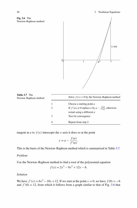
56 3 Nonlinear Equations
Fig. 3.6 TheNewton–Raphson method
Table 3.7 TheNewton–Raphson method Solve f (x) = 0 by the Newton–Raphson method
1 Choose a starting point a
2 If f ′(a) �= 0 replace a by a − f (a)f ′(a)
otherwise
restart using a different a
3 Test for convergence
4 Repeat from step 2
tangent at a to f (x) intercepts the x-axis it does so at the point
x = a − f (a)
f ′(a).
This is the basis of the Newton–Raphson method which is summarised in Table 3.7.
Problem
Use the Newton–Raphson method to find a root of the polynomial equation
f (x) = 2x3 − 9x2 + 12x − 6.
Solution
We have f ′(x) = 6x2 −18x +12. If we start at the point x = 0, we have f (0) = −6and f ′(0) = 12, from which it follows from a graph similar to that of Fig. 3.6 that
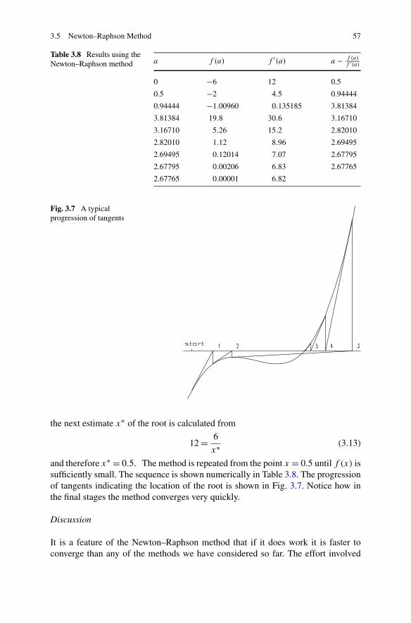
3.5 Newton–Raphson Method 57
Table 3.8 Results using theNewton–Raphson method a f (a) f ′(a) a − f (a)
f ′(a)
0 −6 12 0.5
0.5 −2 4.5 0.94444
0.94444 −1.00960 0.135185 3.81384
3.81384 19.8 30.6 3.16710
3.16710 5.26 15.2 2.82010
2.82010 1.12 8.96 2.69495
2.69495 0.12014 7.07 2.67795
2.67795 0.00206 6.83 2.67765
2.67765 0.00001 6.82
Fig. 3.7 A typicalprogression of tangents
the next estimate x∗ of the root is calculated from
12 = 6
x∗ (3.13)
and therefore x∗ = 0.5. The method is repeated from the point x = 0.5 until f (x) issufficiently small. The sequence is shown numerically in Table 3.8. The progressionof tangents indicating the location of the root is shown in Fig. 3.7. Notice how inthe final stages the method converges very quickly.
Discussion
It is a feature of the Newton–Raphson method that if it does work it is faster toconverge than any of the methods we have considered so far. The effort involved
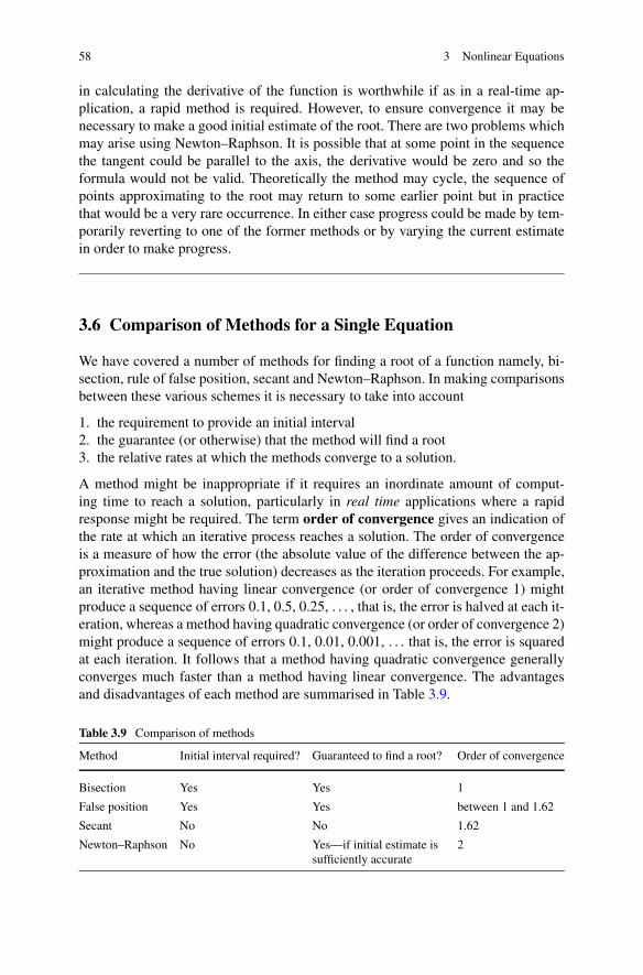
58 3 Nonlinear Equations
in calculating the derivative of the function is worthwhile if as in a real-time ap-plication, a rapid method is required. However, to ensure convergence it may benecessary to make a good initial estimate of the root. There are two problems whichmay arise using Newton–Raphson. It is possible that at some point in the sequencethe tangent could be parallel to the axis, the derivative would be zero and so theformula would not be valid. Theoretically the method may cycle, the sequence ofpoints approximating to the root may return to some earlier point but in practicethat would be a very rare occurrence. In either case progress could be made by tem-porarily reverting to one of the former methods or by varying the current estimatein order to make progress.
3.6 Comparison of Methods for a Single Equation
We have covered a number of methods for finding a root of a function namely, bi-section, rule of false position, secant and Newton–Raphson. In making comparisonsbetween these various schemes it is necessary to take into account
1. the requirement to provide an initial interval2. the guarantee (or otherwise) that the method will find a root3. the relative rates at which the methods converge to a solution.
A method might be inappropriate if it requires an inordinate amount of comput-ing time to reach a solution, particularly in real time applications where a rapidresponse might be required. The term order of convergence gives an indication ofthe rate at which an iterative process reaches a solution. The order of convergenceis a measure of how the error (the absolute value of the difference between the ap-proximation and the true solution) decreases as the iteration proceeds. For example,an iterative method having linear convergence (or order of convergence 1) mightproduce a sequence of errors 0.1, 0.5, 0.25, . . . , that is, the error is halved at each it-eration, whereas a method having quadratic convergence (or order of convergence 2)might produce a sequence of errors 0.1, 0.01, 0.001, . . . that is, the error is squaredat each iteration. It follows that a method having quadratic convergence generallyconverges much faster than a method having linear convergence. The advantagesand disadvantages of each method are summarised in Table 3.9.
Table 3.9 Comparison of methods
Method Initial interval required? Guaranteed to find a root? Order of convergence
Bisection Yes Yes 1
False position Yes Yes between 1 and 1.62
Secant No No 1.62
Newton–Raphson No Yes—if initial estimate issufficiently accurate
2
3.7 Newton’s Method for Systems of Nonlinear Equations 59
3.7 Newton’s Method for Systems of Nonlinear Equations
To take matters further we consider nonlinear relationships involving more than onevariable. We restrict our attention to systems of equations having the same numberof equations as unknowns. Systems having an unequal number of equations andunknowns can be dealt with as an optimisation problem (Chap. 8). We write thesystem as
f(x) = 0.
By way of an example we consider the following problem.
Problem
The stress distribution within a metal plate under a uniformly distributed load ismodelled by (3.14) and (3.15). The variables x1 and x2 define the position of a pointwithin the plate, but the precise details need not concern us.
f1(x1, x2) = cos(2x1) − cos(2x2) − 0.4 (3.14)
f2(x1, x2) = 2(x2 − x1) + sin(2x2) − sin(2x1) − 1.2. (3.15)
The problem is to find values for x1 and x2 such that f1(x1, x2) = f2(x1, x2) = 0.Although it is possible to extend the secant method to deal with such systems byusing planes in 3-dimensional space rather than secants in 2-dimensional space it iseasier to extend the principles of the Newton–Raphson method into what is knownas Newton’s method.
Solution
As usual we start from some initial approximation to the roots. In this case wechoose x1 = 0.1 and x2 = 0.5. These are values which, given a familiarity withthe problem being modelled, are not unreasonable. In any event f1(0.1,0.5) ≈ 0.04and f2 ≈ 0.2 and are therefore reasonably close to zero. In dealing with systemsof nonlinear equations it is as well to exercise some care in choosing the initialapproximations since in general the methods for nonlinear systems are not as robustas those for single equations and may not work for initial approximations too farfrom the solution. Given the initial points x1 = 0.1 and x2 = 0.5 we look for a betterapproximation x∗
1 and x∗2 to make f1(x
∗1 , x∗
2 ) and f2(x∗1 , x∗
2 ) closer to the root.If the function f1 is plotted on the axes shown in Fig. 3.8 we have a 3-dimensional
shape at which the point marked A has coordinates (0.1,0.5) in the (x1, x2) plane.We attempt to follow the shape of the function f1 in the x1 = 0.1 plane by drawingthe tangent AB to f1 at (0.1,0.5). Similarly, we follow the shape in the x2 = 0.5plane by drawing the tangent AC to f1 at (0.1,0.5). Since we are dealing with asolid shape, there are many tangents at any particular point. As yet the points B andC are undefined but we aim to construct a point D in the plane of f1 = 0 such thatCD is parallel to AB, and AC, FG and BD are parallel. The shape ABCD is ourapproximation to f1 even though at this stage the point D is not uniquely defined.
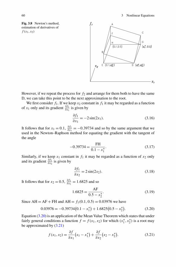
60 3 Nonlinear Equations
Fig. 3.8 Newton’s method,estimation of derivatives off (x1, x2)
However, if we repeat the process for f2 and arrange for them both to have the sameD, we can take this point to be the next approximation to the root.
We first consider f1. If we keep x2 constant in f1 it may be regarded as a functionof x1 only and its gradient ∂f1
∂x1is given by
∂f1
∂x1= −2 sin(2x1). (3.16)
It follows that for x1 = 0.1, ∂f1∂x1
= −0.39734 and so by the same argument that weused in the Newton–Raphson method for equating the gradient with the tangent ofthe angle
−0.39734 = FH
0.1 − x∗1. (3.17)
Similarly, if we keep x1 constant in f1 it may be regarded as a function of x2 onlyand its gradient ∂f1
∂x2is given by
∂f1
∂x2= 2 sin(2x2). (3.18)
It follows that for x2 = 0.5, ∂f1∂x1
= 1.6825 and so
1.6825 = AF
0.5 − x∗2. (3.19)
Since AH = AF + FH and AH = f1(0.1,0.5) = 0.03976 we have
0.03976 = −0.39734(0.1 − x∗
1
) + 1.6825(0.5 − x∗
2
). (3.20)
Equation (3.20) is an application of the Mean Value Theorem which states that underfairly general conditions a function f = f (x1, x2) for which (x∗
1 , x∗2 ) is a root may
be approximated by (3.21)
f (x1, x2) = ∂f
∂x1
(x1 − x∗
1
) + ∂f
∂x2
(x2 − x∗
2
). (3.21)
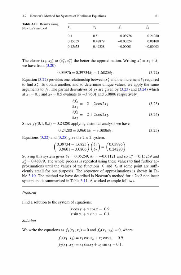
3.7 Newton’s Method for Systems of Nonlinear Equations 61
Table 3.10 Results usingNewton’s method x1 x2 f1 f2
0.1 0.5 0.03976 0.24280
0.15259 0.48879 −0.00524 0.00108
0.15653 0.49338 −0.00001 −0.00003
The closer (x1, x2) to (x∗1 , x∗
2 ) the better the approximation. Writing x∗1 = x1 + δ1
we have from (3.20)
0.03976 = 0.39734δ1 − 1.6825δ2. (3.22)
Equation (3.22) provides one relationship between x∗1 and the increment δ1 required
to find x∗2 . To obtain another, and so determine unique values, we apply the same
arguments to f2. The partial derivatives of f2 are given by (3.23) and (3.24) whichat x1 = 0.1 and x2 = 0.5 evaluate to −3.9601 and 3.0806 respectively.
∂f2
∂x1= −2 − 2 cos 2x1 (3.23)
∂f2
∂x2= 2 + 2 cos 2x2. (3.24)
Since f2(0.1,0.5) = 0.24280 applying a similar analysis we have
0.24280 = 3.9601δ1 − 3.0806δ2. (3.25)
Equations (3.22) and (3.25) give the 2 × 2 system:(
0.39734 − 1.68253.9601 − 3.0806
)(δ1δ2
)=
(0.039760.24280
).
Solving this system gives δ1 = 0.05259, δ2 = −0.01121 and so x∗1 = 0.15259 and
x∗2 = 0.48879. The whole process is repeated using these values to find further ap-
proximations until the values of the functions f1 and f2 at some point are suffi-ciently small for our purposes. The sequence of approximations is shown in Ta-ble 3.10. The method we have described is Newton’s method for a 2×2 nonlinearsystem and is summarised in Table 3.11. A worked example follows.
Problem
Find a solution to the system of equations:
x cosy + y cosx = 0.9x siny + y sinx = 0.1.
Solution
We write the equations as f1(x1, x2) = 0 and f2(x1, x2) = 0, where
f1(x1, x2) = x1 cosx2 + x2 cosx1 − 0.9
f2(x1, x2) = x1 sinx2 + x2 sinx1 − 0.1.
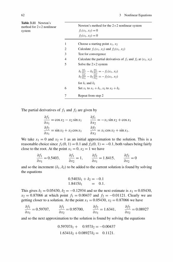
62 3 Nonlinear Equations
Table 3.11 Newton’smethod for 2×2 nonlinearsystem
Newton’s method for the 2×2 nonlinear system
f1(x1, x2) = 0
f2(x1, x2) = 0
1 Choose a starting point x1, x2
2 Calculate f1(x1, x2) and f2(x1, x2)
3 Test for convergence
4 Calculate the partial derivatives of f1 and f2 at (x1, x2)
5 Solve the 2×2 system
δ1∂f1∂x1
− δ2∂f1∂x2
= −f1(x1, x2)
δ2∂f2∂x1
− δ2∂f2∂x2
= −f2(x1, x2)
for δ1 and δ2
6 Set x1 to x1 + δ1, x2 to x2 + δ2
7 Repeat from step 2
The partial derivatives of f1 and f2 are given by
∂f1
∂x1= cosx2 − x2 sinx1
∂f1
∂x2= −x1 sinx2 + cosx1
∂f2
∂x1= sinx2 + x2 cosx1
∂f2
∂x2= x1 cosx2 + sinx1.
We take x1 = 0 and x2 = 1 as an initial approximation to the solution. This is areasonable choice since f1(0,1) = 0.1 and f2(0,1) = −0.1, both values being fairlyclose to the root. At the point x1 = 0, x2 = 1 we have
∂f1
∂x1= 0.5403,
∂f1
∂x2= 1,
∂f2
∂x1= 1.8415,
∂f2
∂x2= 0
and so the increment (δ1, δ2) to be added to the current solution is found by solvingthe equations
0.5403δ1 + δ2 = −0.11.8415δ1 = 0.1.
This gives δ1 = 0.05430, δ2 = −0.12934 and so the next estimate is x1 = 0.05430,x2 = 0.87066 at which point f1 = 0.00437 and f2 = −0.01121. Clearly we aregetting closer to a solution. At the point x1 = 0.05430, x2 = 0.87066 we have
∂f1
∂x1= 0.59707,
∂f1
∂x2= 0.95700,
∂f2
∂x1= 1.6341,
∂f2
∂x2= 0.08927
and so the next approximation to the solution is found by solving the equations
0.59707δ1 + 0.957δ2 = −0.00437
1.6341δ2 + 0.08927δ2 = 0.1121.
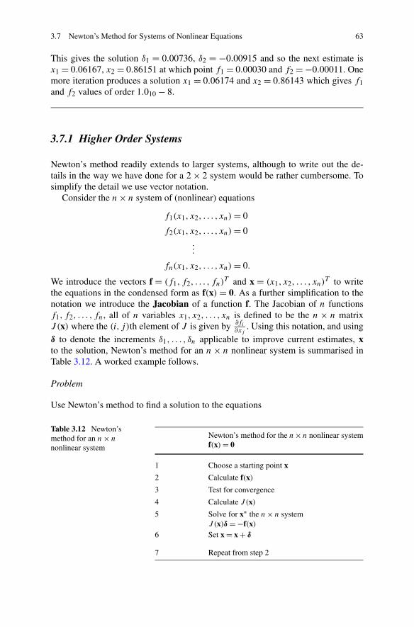
3.7 Newton’s Method for Systems of Nonlinear Equations 63
This gives the solution δ1 = 0.00736, δ2 = −0.00915 and so the next estimate isx1 = 0.06167, x2 = 0.86151 at which point f1 = 0.00030 and f2 = −0.00011. Onemore iteration produces a solution x1 = 0.06174 and x2 = 0.86143 which gives f1and f2 values of order 1.010 − 8.
3.7.1 Higher Order Systems
Newton’s method readily extends to larger systems, although to write out the de-tails in the way we have done for a 2 × 2 system would be rather cumbersome. Tosimplify the detail we use vector notation.
Consider the n × n system of (nonlinear) equations
f1(x1, x2, . . . , xn) = 0
f2(x1, x2, . . . , xn) = 0...
fn(x1, x2, . . . , xn) = 0.
We introduce the vectors f = (f1, f2, . . . , fn)T and x = (x1, x2, . . . , xn)
T to writethe equations in the condensed form as f(x) = 0. As a further simplification to thenotation we introduce the Jacobian of a function f. The Jacobian of n functionsf1, f2, . . . , fn, all of n variables x1, x2, . . . , xn is defined to be the n × n matrixJ (x) where the (i, j)th element of J is given by ∂fi
∂xj. Using this notation, and using
δ to denote the increments δ1, . . . , δn applicable to improve current estimates, xto the solution, Newton’s method for an n × n nonlinear system is summarised inTable 3.12. A worked example follows.
Problem
Use Newton’s method to find a solution to the equations
Table 3.12 Newton’smethod for an n × n
nonlinear system
Newton’s method for the n × n nonlinear systemf(x) = 0
1 Choose a starting point x
2 Calculate f(x)
3 Test for convergence
4 Calculate J (x)
5 Solve for x∗ the n × n systemJ (x)δ = −f(x)
6 Set x = x + δ
7 Repeat from step 2
64 3 Nonlinear Equations
3 + 2
r2− 1
8
(3 − 2v)
1 − vω2r2 = 4.5
6v − 1
2
v
1 − vω2r2 = 2.5
3 − 2
r2− 1
8
(1 + 2v)
1 − vω2r2 = 0.5.
These equations arise in the modelling of stress on a turbine rotor.
Solution
Modifying the notation so that v, ω and r become x1, x2 and x3 respectively, andintroducing f = (f1, f2, f3)
T we solve the system f(x) = 0, where
f1 = 3 + 2
x23
− 1
8
(3 − 2x1)
1 − x1x2
2x23 − 4.5
f2 = 6x1 − 1
2
x1
1 − x1x2
2x23 − 2.5
f3 = 3 − 2
x23
− 1
8
(1 + 2x1)
1 − x1x2
2x23 − 0.5.
The Jacobian of these functions is given by
J =
⎛
⎜⎜⎜⎜⎜⎝
− x22x2
3
8(1−x1)2 − (3−2x1)x2x
23
4(1−x1)− 4
x23
− (3−2x1)x22x3
4(1−x1)
6 + x22x2
3
2(1−x1)2 − x1x2x
23
1−x1− x1x
22x3
1−x1
− 3x22x2
3
8(1−x1)2 − (1+2x1)x2x
23
4(1−x1)4x2
3− (1+2x1)x
22x3
4(1−x1)
⎞
⎟⎟⎟⎟⎟⎠
.
Starting with estimates x1 = 0.75, x2 = 0.5, x3 = 0.5, we find that
J =⎛
⎝−0.1250 −0.0469 −16.1875
6.5000 −0.3750 −0.3750−0.3750 −0.3125 15.6875
⎞
⎠ .
To find the next estimate we use Gaussian elimination to solve the 3 × 3 linearsystem
J(x)δ = −f(x)
where x is the current, to find δ = (−0.1497,2.0952,0.3937) which we add to x togive the next estimate. The process is repeated until function values f1, f2 and f3
are sufficiently small. Results are shown in Table 3.13.
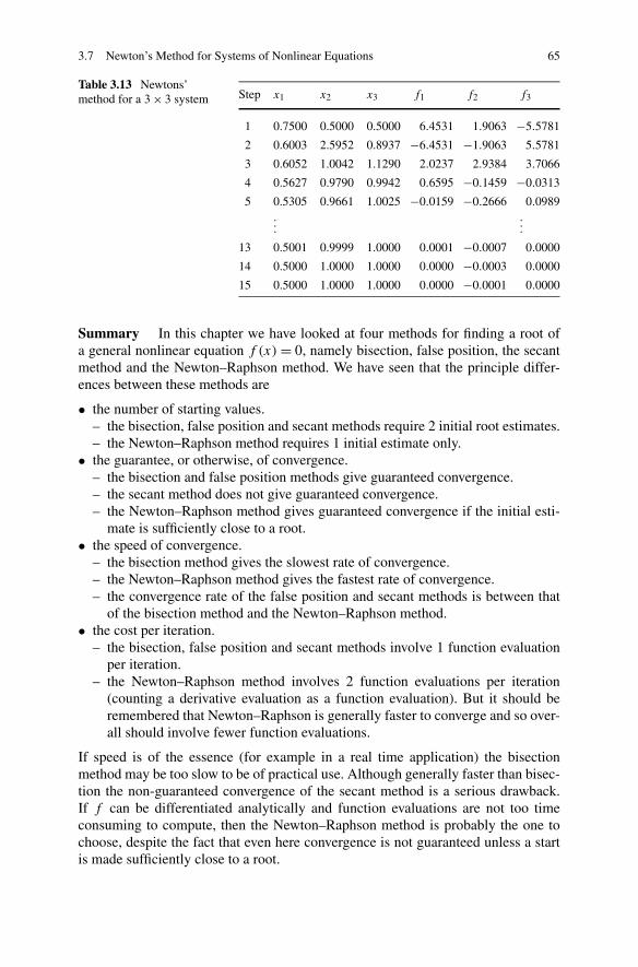
3.7 Newton’s Method for Systems of Nonlinear Equations 65
Table 3.13 Newtons’method for a 3 × 3 system Step x1 x2 x3 f1 f2 f3
1 0.7500 0.5000 0.5000 6.4531 1.9063 −5.5781
2 0.6003 2.5952 0.8937 −6.4531 −1.9063 5.5781
3 0.6052 1.0042 1.1290 2.0237 2.9384 3.7066
4 0.5627 0.9790 0.9942 0.6595 −0.1459 −0.0313
5 0.5305 0.9661 1.0025 −0.0159 −0.2666 0.0989...
.
.
.
13 0.5001 0.9999 1.0000 0.0001 −0.0007 0.0000
14 0.5000 1.0000 1.0000 0.0000 −0.0003 0.0000
15 0.5000 1.0000 1.0000 0.0000 −0.0001 0.0000
Summary In this chapter we have looked at four methods for finding a root ofa general nonlinear equation f (x) = 0, namely bisection, false position, the secantmethod and the Newton–Raphson method. We have seen that the principle differ-ences between these methods are
• the number of starting values.– the bisection, false position and secant methods require 2 initial root estimates.– the Newton–Raphson method requires 1 initial estimate only.
• the guarantee, or otherwise, of convergence.– the bisection and false position methods give guaranteed convergence.– the secant method does not give guaranteed convergence.– the Newton–Raphson method gives guaranteed convergence if the initial esti-
mate is sufficiently close to a root.• the speed of convergence.
– the bisection method gives the slowest rate of convergence.– the Newton–Raphson method gives the fastest rate of convergence.– the convergence rate of the false position and secant methods is between that
of the bisection method and the Newton–Raphson method.• the cost per iteration.
– the bisection, false position and secant methods involve 1 function evaluationper iteration.
– the Newton–Raphson method involves 2 function evaluations per iteration(counting a derivative evaluation as a function evaluation). But it should beremembered that Newton–Raphson is generally faster to converge and so over-all should involve fewer function evaluations.
If speed is of the essence (for example in a real time application) the bisectionmethod may be too slow to be of practical use. Although generally faster than bisec-tion the non-guaranteed convergence of the secant method is a serious drawback.If f can be differentiated analytically and function evaluations are not too timeconsuming to compute, then the Newton–Raphson method is probably the one tochoose, despite the fact that even here convergence is not guaranteed unless a startis made sufficiently close to a root.

66 3 Nonlinear Equations
Finally we looked at Newton’s method for systems of equations which weshowed to be an extension of the Newton–Raphson method.
Exercises
1. Write a Matlab program to find√
2 using the bisection method. Do this by find-ing a root of the function f (x) = x2 −2 in the interval [1,2]. Aim for an accuracyof 4 decimal places. Write Matlab code based on the following which shows theinterval containing the root shrinking to a point at which it has length less than0.00005. The code assumes that the function sq2(x) to evaluate x2 − 2 has beenestablished in an M-file sq2.m (see Sect. 1.5).
low = 1; % initial lower boundhigh = 2; % initial upper boundwhile high− low > 0.00005;
mid = (high + low)/2; % mid point of current boundsif sq2(low)∗sq2(mid) < 0 % solution lies to the left
high = mid;else % solution lies to the right
low = mid;end;s = sprintf('solution lies in [%8.4f,%8.4f]', low, high);disp(s);
end;
2. Use the following code to plot the function f (x) = x sinx − cosx to show thatit has just one root in the interval [0,π/2].% construct 50 x-points equally spaced between 0 and pi/2
x = linspace(0, pi/2, 50);% use element by element multiplication to form x sin(x)
y = x.∗sin(x) - cos(x);plot(x,y);
Modify the code from question 1 to find the root of f (x) = x sin(x) − cos(s) in[0,π/2] to an accuracy of four decimal places. Check the result using the Matlabfunction fzero. A suitable command would be
solution = fzero(@fsincos, 1.0)
where the function fsincos(x) = x sin(x) − cos(x) is defined in the M-filefsincos.m. Note how the name of the function, fsincos is passed to fzero usingthe @ symbol. The second parameter of fzero supplies a starting estimate of thesolution.
3. Modify the code for the bisection method (question 1) to implement the methodof false position. Replace the variable name mid by a more meaningful namesuch as xstar, where xstar is calculated using the (3.7). Modify the conditionfor the while loop to terminate. Test the code by finding
√2 to an accuracy of 4
decimal places.
3.7 Newton’s Method for Systems of Nonlinear Equations 67
4. Use the following code as the basis for writing a Matlab program to find a rootof the function f (x) = 0 using the secant method.
% Secant method for solving f(x)=0% Assume estimates a and b, the required accuracy eps and function f have% been defined
while abs(f(xstar)) > epsxstar = b - f(b)∗(a-b)/(f(a)-f(b));a = b;b = xstar;
end;disp(xstar);
Test the program by finding√
2 to 4 decimal places using starting estimates (i)a = 1, b = 2 to find the positive root and (ii) a = −1, b = −2 to find the negativeroot.
5. By plotting a suitable graph show that the polynomial 4x3 − 8x2 + 3x − 10has only one real root. Use the secant program developed in question 4 to findthis root. Display successive approximations to show progress to the solution.Because of the nature of the function as shown in the plot, progress may berather slow for certain initial estimates. For estimates a = −0.5, b = −1 themethod fails, but with a plot to hand this would be an unlikely choice.
Check the solution using the Matlab function roots which finds all the roots ofa polynomial. The input to the function is a vector of coefficients in left to rightorder. For the quoted example a Matlab command
roots([ 4 −8 3 −10])
would be appropriate.6. Write a Matlab program to find
√2 using the Newton–Raphson method. As be-
fore do this by finding a root of the function f (x) = x2 − 2. You will see that themethod is equivalent to continually replacing the current estimate x, of
√2, by a
new estimate ( x2 + 1
x).
Consider the more general problem of finding the pth root of a number a,(p, a positive real numbers) by using the Newton–Raphson method to find a rootof the function f (x) = xp − a. Test the program on examples such as 81/3 and22/5. Compare with the values expressed by Matlab commands.
7. Write a general purpose Matlab function Newton–Raphson to find a root of agiven function f , where f and its derivative f ′ are defined as Matlab functionsin the M-files f.m and fdash.m respectively. The Newton–Raphson function isto have input parameters estimate, an estimate of the solution, abs the requiredabsolute accuracy of the solution and limit a limit on the number of iterations.
The following is a suggestion for the form of the function:
function [root] = Newton–Raphson(estimate, eps, limit)x = estimate;count = 0;while diff > eps && count < limit
68 3 Nonlinear Equations
if fdash(x) ∼= 0root = x - f(x)/fdash(x);diff = abs(root-x);x = root;count = count + 1;
else% Print a diagnostic message to show why the procedure has failed
s = sprintf('Method fails, zero derivative at %8.4f ', x);disp(s);break;
end;
Notice how the break command has been used to return prematurely from thewhile loop and in this case return to the calling program.
Test the program using the function of question 5. Notice how Newton–Raphson generally requires fewer iterations than the Secant method.
8. Write a Matlab program to find a solution to the following system of equations.Use Newton’s method for a 2 × 2 system following the scheme to verify theresults shown in Sect. 3.7
x1 cosx2 + x2 cosx1 = 0.9
x1 sinx2 + x2 sinx1 = 0.1.
A suitable program might have the form
x = [0 ; 1] % initial estimate of the solutionfor i = 1 : 3 % perform three iterations% form the matrix of coefficientsA = [diff1(x,1) diff1(x,2) ; diff2(x,1) diff2(x,2)];% right hand sideb = −[ f1(x) ; f2(x)]d = A\b; % solve the equationsx = x + d % next estimate
end;
Matlab provides the function fsolve to find a solution of a system of non-linearequations. The function provides many options but for this example the followingprogram would be appropriate.
x0 = [ 0 ; 1 ]; % initial estimateoptions=optimset('Display','iter'); % options to display the iterative process[x] = fsolve(@sys,x0,options) % solution returned in vector x
where it is assumed that the system of equations is defined as the function sys inthe Matlab M-file sys.m as follows
function eqns = sys(x)eqns = [ x(1)∗cos(x(2)) + x(2)∗cos(x(1)) −0.9;
x(1)∗sin(x(2)) + x(2)∗sin(x(1)) −0.1 ];

3.7 Newton’s Method for Systems of Nonlinear Equations 69
9. Write a Matlab program to find a solution to the following system of equations.Use Newton’s method for an n × n system following the scheme shown in Ta-ble 3.12.
4x21 + 2x2 = 4
x1 + 2x22 + 2x3 = 4
x2 + 2x23 = 4.
Alternatively use the Matlab function fsolve as described in the previous questionwith the equations stored in column vector form as shown below.
% storing the equations in column vector eqns:eqns = [ 4∗x(1)∧2 + 2∗x(2) - 4;
x(1) + 2∗x(2)∧2 + 2∗x(3) - 4;x(2) + 2∗x(3)∧2 - 4 ].
Chapter 4Curve Fitting
Aims In this chapter we look at ways of fitting a smooth curve to supplied datapoints. That is, given a set of pairs of values (xi, yi), we construct a continuousfunction y = f (x) that in some sense represents an underlying function impliedby the data points. Having produced such an approximating function we could forexample, estimate a value for f (x) where x is not one of the xi .
Overview Initially we consider using a straight line as the approximating func-tion. We then consider using polynomials as approximating functions and how wemight find appropriate values for polynomial coefficients. Finally we consider usingmore general functions for approximating purposes and in so doing introduce themethod of least squares approximation. In developing the various methods we takeaccount of whether the approximating function, f (x) is required to fit the data ex-actly or not. It may be possible to produce a simpler, smoother approximation andone more amenable to further analysis and application by allowing a more approxi-mate fit to the data. In practice this is not an inappropriate approach as data collectedfrom observation or experiment may contain error or may have limited accuracy. Inproducing an underlying approximation having such desirable features we may beimproving the accuracy of the data and possibly identifying and eradicating error.
Acquired Skills After reading this chapter you will understand how data maybe represented by a function which may then be used to approximate in-betweenand beyond the given data. You will be able to assess the type of function required,whether linear, polynomial or other, in a given situation. You will be able to con-struct the function, choosing from one of a number of methods appropriate to theproblem under consideration.
4.1 Introduction
Curve fitting is the process whereby a continuous function is constructed in sucha way that it represents supplied data. The main problem is that of deciding what
C. Woodford, C. Phillips, Numerical Methods with Worked Examples: Matlab Edition,DOI 10.1007/978-94-007-1366-6_4, © Springer Science+Business Media B.V. 2012
71

72 4 Curve Fitting
form the continuous function should take. A linear function may be suitable for themeasurement of temperature, but not for measuring gas volume against pressure.For the latter we find that a polynomial is a more suitable function. It may be tempt-ing to assume that in general a higher order polynomial is likely to offer a betterapproximation than a polynomial of lower order, but this is not necessarily so. In-deed, the converse may apply. However, rather than discard polynomials entirely,we show how they can be combined in a piecewise manner to form good approxi-mating functions. Such functions are known as spline functions. We begin by usingstraight line (linear approximation) to fit exactly to given data.
4.2 Linear Interpolation
The temperature of a liquid can be determined by reading a non-digital mercurythermometer. The length of the mercury column may well coincide with one of thecalibration points, but more typically it will lie somewhere between two such points(a lower and an upper bound).
Problem
How might we measure temperatures using a non-digital mercury thermometerwhich is marked at 10° intervals in the range 0° to 100°?
Solution
We estimate the length of the mercury column above the lower point as a fractionof the distance between the lower point and the upper point. The temperature of theliquid is assumed to be the value at the lower of the two points plus the fractiontimes the interval between two calibrations (10°).
A graphical representation of this process (Fig. 4.1) is an x-y plot in which they-axis represents the length of the mercury column and the x-axis represents tem-perature. At the calibration points (temperatures in the range 0° to 100° in steps of10°) we plot the known values of the length of the mercury column on a graph.Assuming suitable consistency conditions are satisfied, such as the cross-section ofthe column is constant throughout the scale portion of the thermometer, the rela-tionship should be linear and we should therefore be able to draw a straight line that(to within the limits of experimental accuracy) links all of the points. Then for anyknown length of the mercury column we simply draw a horizontal line across fromthe appropriate point on the y-axis, and where this meets our straight line we draw avertical line; the point at which this line crosses the x-axis defines the temperature.In this case the fitted curve (albeit a straight line) is a representation of the data sup-plied as lengths of the mercury column (the function values) at temperatures (theindependent variable) in the range 0° to 100° in steps of 10°.
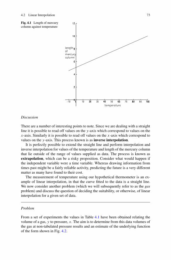
4.2 Linear Interpolation 73
Fig. 4.1 Length of mercurycolumn against temperature
Discussion
There are a number of interesting points to note. Since we are dealing with a straightline it is possible to read off values on the y-axis which correspond to values on thex-axis. Similarly it is possible to read off values on the x-axis which correspond tovalues on the y-axis. This process known is as inverse interpolation.
It is perfectly possible to extend the straight line and perform interpolation andinverse interpolation for values of the temperature and length of the mercury columnthat lie outside of the range of values supplied as data. The process is known asextrapolation, which can be a risky proposition. Consider what would happen ifthe independent variable were a time variable. Whereas drawing information fromtimes past might be a fairly reliable activity, predicting the future is a very differentmatter as many have found to their cost.
The measurement of temperature using our hypothetical thermometer is an ex-ample of linear interpolation, in that the curve fitted to the data is a straight line.We now consider another problem (which we will subsequently refer to as the gasproblem) and discuss the question of deciding the suitability, or otherwise, of linearinterpolation for a given set of data.
Problem
From a set of experiments the values in Table 4.1 have been obtained relating thevolume of a gas, y to pressure, x. The aim is to determine from this data volumes ofthe gas at non-tabulated pressure results and an estimate of the underlying functionof the form shown in Fig. 4.2.
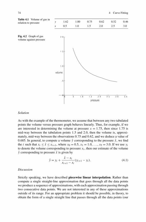
74 4 Curve Fitting
Table 4.1 Volume of gas inrelation to pressure y 1.62 1.00 0.75 0.62 0.52 0.46
x 0.5 1.0 1.5 2.0 2.5 3.0
Fig. 4.2 Graph of gasvolume against pressure
Solution
As with the example of the thermometer, we assume that between any two tabulatedpoints the volume versus pressure graph behaves linearly. Thus, for example, if weare interested in determining the volume at pressure x = 1.75, then since 1.75 ismid-way between the tabulation points 1.5 and 2.0, then the volume is, approxi-mately, mid-way between the observations 0.75 and 0.62, and we deduce a value of0.685. In general, to compute a volume y corresponding to the pressure x, we findthe i such that xi ≤ x ≤ xi+1, where x0 = 0.5, x1 = 1.0, . . . , x5 = 3.0. If we use yi
to denote the volume corresponding to pressure xi , then our estimate of the volumey corresponding to pressure x is given by
y = yi + x − xi
xi+1 − xi
(yi+1 − yi). (4.1)
Discussion
Strictly speaking, we have described piecewise linear interpolation. Rather thancompute a single straight-line approximation that goes through all the data pointswe produce a sequence of approximations, with each approximation passing throughtwo consecutive data points. We are not interested in any of these approximationsoutside of its range. For an appropriate problem it should be possible, in theory, toobtain the form of a single straight line that passes through all the data points (our
4.2 Linear Interpolation 75
thermometer problem can be classified as an appropriate problem). In practice thesituation is less clear; there may well be observational error in the data.
4.2.1 Differences
The accuracy of piecewise linear interpolation will depend on the accuracy of thesupplied data and that the relationship between dependent and independent variablesis linear. The validity or otherwise of the latter can be deduced by forming what areknown as divided differences (or just differences), and this in turn provides theroute to alternative methods of solution. We illustrate the method by constructing atable of differences for the following example.
In an experiment designed to demonstrate the relationship between time and theaverage number of goals scored by a football club per game, a set of results overa playing season was obtained and summarised in Table 4.2. We might deduce thatthe average number of goals scored after 45 minutes is 0.8 + 45−40
50−40 (1.0 − 0.8) =0.9, provided that the relationship between time and goals scored is linear but thatis yet to be established. Let the function values (average number of goals) be yi
corresponding to the points (time duration) xi . Then the divided difference involvingthe two consecutive values yi+1 and yi is simply the difference yi+1 −yi divided byxi+1 − xi . Divided differences corresponding to the data of Table 4.2 are shown inthe third column of Table 4.3; we observe that they all have the same value (0.02).The divided differences themselves can be regarded as y-values, and hence we canconstruct another set of differences (second differences), shown in the fourth columnof Table 4.3. Note that in order to produce these second differences we must fan backto the first column to determine the divisor. Hence, for example, the first entry in thefinal column is found as 0.2−0.2
20−0 . Since the first differences are identical, the seconddifferences are all zero (and so here the actual form of the divisor is not important).
To realise the importance of the difference table, we know from Taylor’s The-orem1 that the first derivative of a function can be approximated by the differ-ence between two function values divided by the difference between values of thepoints at which those function values were obtained. Obtaining a set of values inthis way, it follows that second derivative approximations can be obtained by form-ing divided differences of first divided differences. If these second differences are
Table 4.2 Average number of goals scored per game
Goals 0.0 0.20 0.4 0.6 0.8 1.0 1.2 1.4 1.6 1.8
Play in minutes 0 10 20 30 40 50 60 70 80 90
1Brook Taylor 1685–1731, published his theorem in 1715 although others were able to make sim-ilar claims. The theorem began to carry his name some fifty years later. He somewhat aggressivelypromoted Newton’s work over that of Leibniz and other European mathematicians.
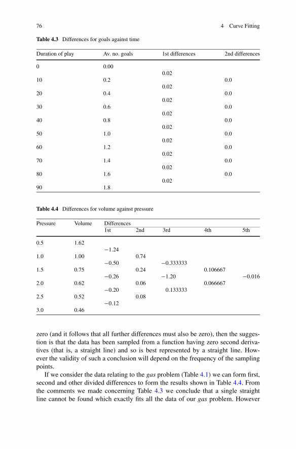
76 4 Curve Fitting
Table 4.3 Differences for goals against time
Duration of play Av. no. goals 1st differences 2nd differences
0 0.000.02
10 0.2 0.00.02
20 0.4 0.00.02
30 0.6 0.00.02
40 0.8 0.00.02
50 1.0 0.00.02
60 1.2 0.00.02
70 1.4 0.00.02
80 1.6 0.00.02
90 1.8
Table 4.4 Differences for volume against pressure
Pressure Volume Differences1st 2nd 3rd 4th 5th
0.5 1.62−1.24
1.0 1.00 0.74−0.50 −0.333333
1.5 0.75 0.24 0.106667−0.26 −1.20 −0.016
2.0 0.62 0.06 0.066667−0.20 0.133333
2.5 0.52 0.08−0.12
3.0 0.46
zero (and it follows that all further differences must also be zero), then the sugges-tion is that the data has been sampled from a function having zero second deriva-tives (that is, a straight line) and so is best represented by a straight line. How-ever the validity of such a conclusion will depend on the frequency of the samplingpoints.
If we consider the data relating to the gas problem (Table 4.1) we can form first,second and other divided differences to form the results shown in Table 4.4. Fromthe comments we made concerning Table 4.3 we conclude that a single straightline cannot be found which exactly fits all the data of our gas problem. However
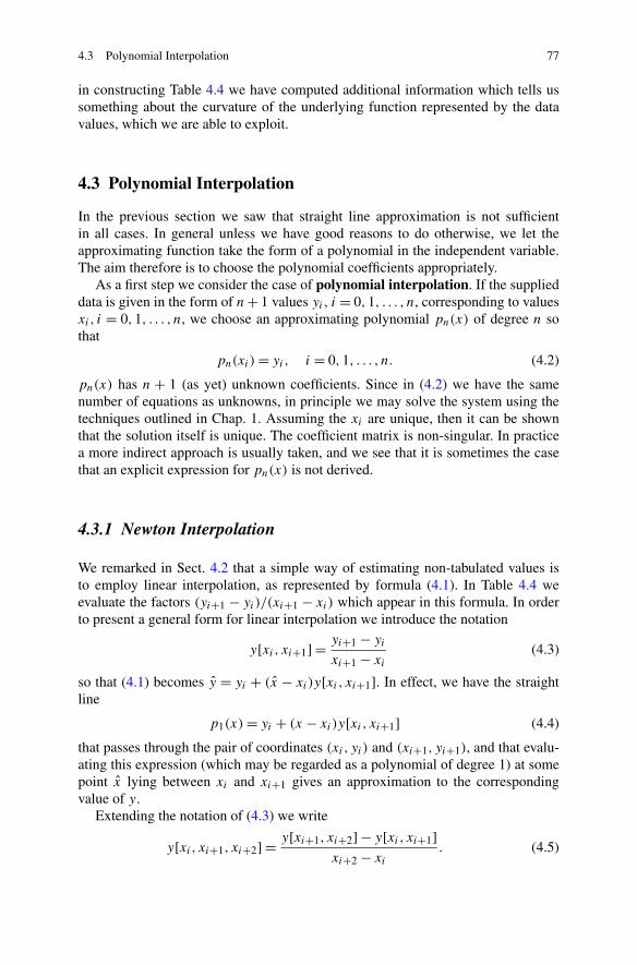
4.3 Polynomial Interpolation 77
in constructing Table 4.4 we have computed additional information which tells ussomething about the curvature of the underlying function represented by the datavalues, which we are able to exploit.
4.3 Polynomial Interpolation
In the previous section we saw that straight line approximation is not sufficientin all cases. In general unless we have good reasons to do otherwise, we let theapproximating function take the form of a polynomial in the independent variable.The aim therefore is to choose the polynomial coefficients appropriately.
As a first step we consider the case of polynomial interpolation. If the supplieddata is given in the form of n + 1 values yi , i = 0,1, . . . , n, corresponding to valuesxi, i = 0,1, . . . , n, we choose an approximating polynomial pn(x) of degree n sothat
pn(xi) = yi, i = 0,1, . . . , n. (4.2)
pn(x) has n + 1 (as yet) unknown coefficients. Since in (4.2) we have the samenumber of equations as unknowns, in principle we may solve the system using thetechniques outlined in Chap. 1. Assuming the xi are unique, then it can be shownthat the solution itself is unique. The coefficient matrix is non-singular. In practicea more indirect approach is usually taken, and we see that it is sometimes the casethat an explicit expression for pn(x) is not derived.
4.3.1 Newton Interpolation
We remarked in Sect. 4.2 that a simple way of estimating non-tabulated values isto employ linear interpolation, as represented by formula (4.1). In Table 4.4 weevaluate the factors (yi+1 − yi)/(xi+1 − xi) which appear in this formula. In orderto present a general form for linear interpolation we introduce the notation
y[xi, xi+1] = yi+1 − yi
xi+1 − xi
(4.3)
so that (4.1) becomes y = yi + (x − xi)y[xi, xi+1]. In effect, we have the straightline
p1(x) = yi + (x − xi)y[xi, xi+1] (4.4)
that passes through the pair of coordinates (xi, yi) and (xi+1, yi+1), and that evalu-ating this expression (which may be regarded as a polynomial of degree 1) at somepoint x lying between xi and xi+1 gives an approximation to the correspondingvalue of y.
Extending the notation of (4.3) we write
y[xi, xi+1, xi+2] = y[xi+1, xi+2] − y[xi, xi+1]xi+2 − xi
. (4.5)
78 4 Curve Fitting
For the gas problem (with i = 0,1,2,3) (4.5) produces the values in the column ofsecond divided differences in Table 4.4. It is not difficult to show that the quadraticpolynomial
p2(x) = yi + (x − xi)y[xi, xi+1] + (x − xi)(x − xi+1)y[xi, xi+1, xi+2] (4.6)
passes through each of the coordinates (xi, yi), (xi+1, yi+1) and (xi+2, yi+2). Thatit passes through the first two of these points follows immediately from our previousconsiderations (the first two terms are just the right-hand side of (4.4) and the finalterm on the right-hand side of (4.6) vanishes at xi and xi+1). The verification ofinterpolation at the third point requires some algebraic manipulation.
We can extend the argument further, and form the kth divided differences as
y[xi, xi+1, . . . , xi+k] = y[xi+1, xi+2, . . . , xi+k] − y[xi, xi+1, . . . , xi+k−1]xi+k − xi
(4.7)
and it can then be established that the polynomial (the Newton interpolating poly-nomial)
pk(x) = yi
+ (x − xi)y[xi, xi+1]+ (x − xi)(x − xi+1)y[xi, xi+1,xi+2]+ · · ·+ (x − xi)(x − xi+1) · · · (x − xi+k−1)y[xi, xi+1, . . . , xi+k] (4.8)
passes through each of the coordinates (xi, yi), (xi+1, yi+1), . . . , (xk, yk). Evaluat-ing this polynomial at some point x between xi and xi+k then gives an approxima-tion to y(x).
Problem
Find the polynomial (the Newton interpolating polynomial) which interpolates thedata given in Table 4.1 (the gas problem). Use this polynomial to estimate the vol-ume of gas at pressure 1.75.
Solution
We have 6 pairs of data (xi, yi), i = 0,1, . . . ,5. Using (4.8) and the appropriatevalues from Table 4.4 we may write the interpolating polynomial as
p5(x) = 1.62
+ (x − 0.5)(−1.24)
+ (x − 0.5)(x − 1.0)(0.74)
+ (x − 0.5)(x − 1.0)(x − 1.5)(−0.333333)
+ (x − 0.5)(x − 1.0)(x − 1.5)(x − 2.0)(0.106667)
+ (x − 0.5)(x − 1.0)(x − 1.5)(x − 2.0)(x − 2.5)(−0.016).
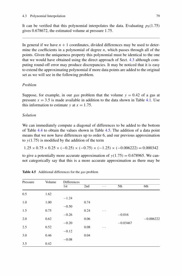
4.3 Polynomial Interpolation 79
It can be verified that this polynomial interpolates the data. Evaluating p5(1.75)
gives 0.678672, the estimated volume at pressure 1.75.
In general if we have n + 1 coordinates, divided differences may be used to deter-mine the coefficients in a polynomial of degree n, which passes through all of thepoints. Given the uniqueness property this polynomial must be identical to the onethat we would have obtained using the direct approach of Sect. 4.3 although com-puting round-off error may produce discrepancies. It may be noticed that it is easyto extend the approximating polynomial if more data points are added to the originalset as we will see in the following problem.
Problem
Suppose, for example, in our gas problem that the volume y = 0.42 of a gas atpressure x = 3.5 is made available in addition to the data shown in Table 4.1. Usethis information to estimate y at x = 1.75.
Solution
We can immediately compute a diagonal of differences to be added to the bottomof Table 4.4 to obtain the values shown in Table 4.5. The addition of a data pointmeans that we now have differences up to order 6, and our previous approximationto y(1.75) is modified by the addition of the term
1.25 × 0.75 × 0.25 × (−0.25) × (−0.75) × (−1.25) × (−0.006222) = 0.000342
to give a potentially more accurate approximation of y(1.75) = 0.678965. We can-not categorically say that this is a more accurate approximation as there may be
Table 4.5 Additional differences for the gas problem
Pressure Volume Differences1st 2nd · · · 5th 6th
0.5 1.62−1.24
1.0 1.00 0.74−0.50
1.5 0.75 0.24 · · ·−0.26 −0.016
2.0 0.62 0.06 −0.006222−0.20 −0.03467
2.5 0.52 0.08 · · ·−0.12
3.0 0.46 0.04−0.08
3.5 0.42
80 4 Curve Fitting
local behaviour around the pressure at point 1.75 which is not reflected in thedata.
4.3.2 Neville Interpolation
In the previous section we observed that it is possible to construct a polynomial,pn(x), of degree n which passes through a sequence of n + 1 coordinates. Havingobtained an explicit form for the polynomial, an interpolated value can then be ob-tained at any required point, and this process can clearly be applied over and overagain.
Neville2 interpolation is an alternative approach that does not yield an explicitform for the interpolating polynomial. Neville’s table yields a single interpolatedvalue, and the table has to be completely reconstructed if interpolation at some otherpoint is required. The method is illustrated in the following problem.
Problem
Use Neville interpolation on the gas problem to estimate a value for y(1.75) fromthe data supplied in Table 4.1.
Solution
For Neville interpolation a table of the form shown in Table 4.6 is constructed.Consider the following rearrangement of the equation for linear interpolation (4.1)
y = (x − xi)yi+1 − (x − xi+1)yi
xi+1 − xi
, i = 0,1, . . . ,5. (4.9)
This formula defines the way in which the values shown in the third column ofTable 4.6 (labelled Linear) have been calculated. Setting x = 1.75 we have for i = 0,((1.75 − 0.5) × 1.00 − (1.75 − 1.0) × 1.62)/(1.0 − 0.5) = 0.07. Similarly, settingi = 1 we find a value 0.625, and so on up to values corresponding to i = 5.
Each entry in the Linear column is an estimate of y(1.75). Only the third isan interpolated approximation since linear interpolation has been performed usingpoints which bracket x. All remaining estimates are based on extrapolated values.
To complete the table we repeat the process using values in one column to pro-ceed to the next. The fourth column of values (labelled Quadratic) is obtained fromthe third column (and the xi ), the fifth column (labelled Cubic) from the fourth col-umn, and so on. The xi+1 in (4.9) is taken to be the x value on the same row asthe element to be computed. The appropriate xi value is found by tracking back
2E.H. Neville, 1889–1961, among many other achievements instrumental in bringing wonder math-ematician Ramanujan to Cambridge to study with the eminent pure mathematician G.H. Hardy.
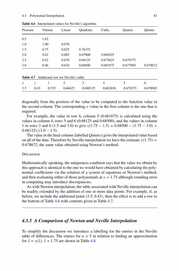
4.3 Polynomial Interpolation 81
Table 4.6 Interpolated values for Neville’s algorithm
Pressure Volume Linear Quadratic Cubic Quartic Quintic
0.5 1.62
1.0 1.00 0.070
1.5 0.75 0.625 0.76375
2.0 0.62 0.685 0.67000 0.685625
2.5 0.52 0.670 0.68125 0.675625 0.679375
3.0 0.46 0.610 0.68500 0.681875 0.677969 0.678672
Table 4.7 Additional row for Neville’s table
x y 1 2 3 4 5 6
3.5 0.43 0.535 0.66625 0.688125 0.682656 0.679375 0.678965
diagonally from the position of the value to be computed to the function value inthe second column. The corresponding x-value in the first column is the one that isrequired.
For example, the value in row 6, column 5 (0.681875) is calculated using thevalues in column 4, rows 5 and 6 (0.68125 and 0.68500), and the values in column1 in rows 3 and 6 (1.5 and 3.0) to give ((1.75 − 1.5) × 0.68500 − (1.75 − 3.0) ×0.68125)/(3.0 − 1.5).
The value in the final column (labelled Quintic) gives the interpolated value basedon all of the data. Therefore by Neville interpolation we have the estimate y(1.75) =0.678672, the same value obtained using Newton’s method.
Discussion
Mathematically speaking, the uniqueness condition says that the value we obtain bythis approach is identical to the one we would have obtained by calculating the poly-nomial coefficients via the solution of a system of equations or Newton’s method,and then evaluating either of those polynomials at x = 1.75 although rounding errorin computing may introduce discrepancies.
As with Newton interpolation, the table associated with Neville interpolation canbe readily extended by the addition of one or more data points. For example, if, asbefore, we include the additional point (3.5,0.43), then the effect is to add a row tothe bottom of Table 4.6 with contents given in Table 4.7.
4.3.3 A Comparison of Newton and Neville Interpolation
To simplify the discussion we introduce a labelling for the entries in the Nevilletable of differences. The entries for n = 5 in relation to finding an approximationfor y = y(x), x = 1.75 are shown in Table 4.8.

82 4 Curve Fitting
Table 4.8 Labelling of interpolated values for Neville’s algorithm
x y Linear Quadratic Cubic Quartic Quintic
x0 y0 = P00
x1 y1 = P10 P11
x2 y2 = P20 P21 P22
x3 y3 = P30 P31 P32 P33
x4 y4 = P40 P41 P42 P43 P44
x5 y5 = P50 P51 P52 P53 P54 P55
Neville’s algorithm, as we have presented it, could be adapted to yield an explicitform for an approximating polynomial, but the entries in the difference table needto be polynomials, rather than just numbers. For example, the entries in the firstcolumn would be linear polynomials, rather than the values of those polynomialsevaluated at an interpolation point, as given in Table 4.6. From (4.9) we deduce thatthe first entry in this column would be
P11(x) = (x − x0)y1 − (x − x1)y0
x1 − x0
whilst the second entry (P21(x)) would be
P21(x) = (x − x1)y2 − (x − x2)y1
x2 − x1.
Looking to the second column, it follows that the first entry would be computedas
P22(x) = (x − x0)P21(x) − (x − x2)P11(x)
x2 − x0(4.10)
and it is clear that this must be a quadratic polynomial. Further, substituting xi ,i = 1,2,3 for x in (4.10) it can be seen that P22(xi) = yi . When evaluated at thepoint x, this polynomial will give the value P22 = 0.76375 of Table 4.6.
It is easy to verify that all of the entries in the column headed ‘Quadratic’ inTable 4.6 are based on quadratic interpolation, in the same way that P22(x) = P22.Similarly, it can be easily shown that entries in subsequent columns are based on cu-bic, quartic and quintic interpolation. It is not surprising therefore, that the potentialmost accurate result produced by Neville interpolation is identical to that obtainedusing Newton interpolation.
Mathematically there is nothing to choose between Neville and Newton interpo-lation, but the two methods have different computational characteristics. If a singleinterpolated value only is required then Neville interpolation will involve consider-ably fewer arithmetic operations than forming and then evaluating the interpolationpolynomial using Newton’s divided difference method. If several interpolated val-ues are required then forming the interpolation polynomial and evaluating it is likelyto be more effective than repeatedly constructing in full the table of Neville’s algo-rithm. Further, the form of the polynomial provided by Newton’s method is cheaperto evaluate than that provided by Neville interpolation.
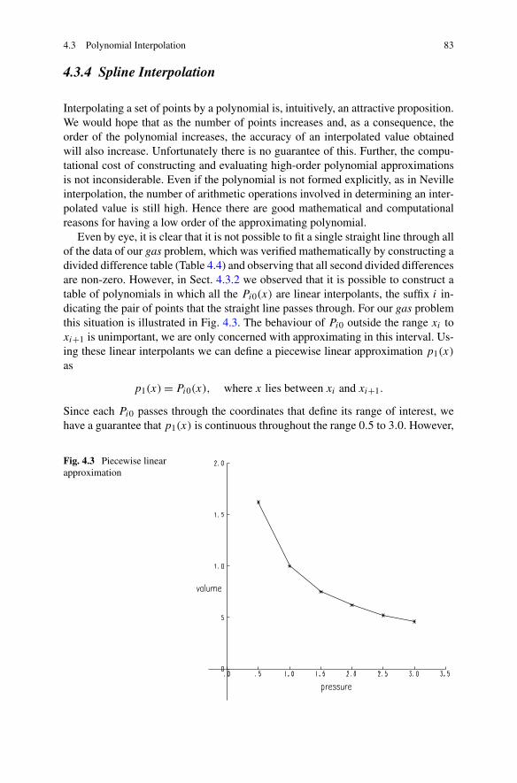
4.3 Polynomial Interpolation 83
4.3.4 Spline Interpolation
Interpolating a set of points by a polynomial is, intuitively, an attractive proposition.We would hope that as the number of points increases and, as a consequence, theorder of the polynomial increases, the accuracy of an interpolated value obtainedwill also increase. Unfortunately there is no guarantee of this. Further, the compu-tational cost of constructing and evaluating high-order polynomial approximationsis not inconsiderable. Even if the polynomial is not formed explicitly, as in Nevilleinterpolation, the number of arithmetic operations involved in determining an inter-polated value is still high. Hence there are good mathematical and computationalreasons for having a low order of the approximating polynomial.
Even by eye, it is clear that it is not possible to fit a single straight line through allof the data of our gas problem, which was verified mathematically by constructing adivided difference table (Table 4.4) and observing that all second divided differencesare non-zero. However, in Sect. 4.3.2 we observed that it is possible to construct atable of polynomials in which all the Pi0(x) are linear interpolants, the suffix i in-dicating the pair of points that the straight line passes through. For our gas problemthis situation is illustrated in Fig. 4.3. The behaviour of Pi0 outside the range xi toxi+1 is unimportant, we are only concerned with approximating in this interval. Us-ing these linear interpolants we can define a piecewise linear approximation p1(x)
as
p1(x) = Pi0(x), where x lies between xi and xi+1.
Since each Pi0 passes through the coordinates that define its range of interest, wehave a guarantee that p1(x) is continuous throughout the range 0.5 to 3.0. However,
Fig. 4.3 Piecewise linearapproximation
84 4 Curve Fitting
there is a change in the value of the slope of p1(x) at each of the internal interpola-tion points (the points 1.0, 1.5, 2.0 and 2.5), as indicated by the different values inthe column of second differences in Table 4.4.
Piecewise linear interpolation is of limited use as it yields only a crude approx-imation to the data. Consideration of the Neville table, with polynomials beingproduced rather than interpolated values, suggests a simple way of increasing theorder of polynomial approximation. P20(x) will be a polynomial interpolating thedata points (0.5,1.62), (1.0,1.00) and (1.5,0.75), P21(x) interpolates at the points(1.0,1.00), (1.5,0.75) and (2.0,0.62), and so on. We therefore have a sequence ofquadratics and can define a piecewise quadratic polynomial p2(x) as being definedby one of the P2i (x), depending on within which of the intervals x lies. We havea slight problem here, in that for all but the first and last intervals there is a choicebetween two quadratics (and the form of these quadratics will be different). Thisdilemma can be avoided by taking the first, third, fifth, etc., but for our gas problemthis simply replaces one problem with another. P22(x) and P42(x) can be used todefine p2(x) within 0.5 to 1.5 and 1.5 to 2.5 respectively, but what about 2.5 to 3.0?Further, whilst we have upped the degree of the approximating polynomial by one(from linear to quadratic), the discontinuity of the first (and, now, second) derivativeremains, so it is not as smooth as maybe we would like.
An alternative approach which increases the degree of polynomial approxima-tion and also improves the continuity characteristics is based on the use of splines.Piecewise linear interpolation is, in fact, a simple example of spline3 approxima-tion. Within each interval we have a local approximating polynomial and the overallapproximation is defined as the aggregate of these individual approximations. Foreach local polynomial of degree n, n + 1 polynomial coefficients will need to bedefined. Suppose that we choose n = 3 (cubic spline interpolation). We look for apiecewise cubic approximation p3(x) such that
p3(x) = p3,i (x), if x lies between xi and xi+1
where p3,i (x) is an approximating cubic between xi and xi+1.
Problem
Use spline interpolation on the gas problem. In particular estimate y(1.75).
Solution
In the first interval we wish to determine values for the coefficients a0, b0, c0 andd0 in a cubic polynomial p3,0(x) ≡ a0 + b0x + c0x
2 + d0x3 such that p3,0(x) is the
approximating polynomial between x = 0.5 and x = 1.0. For p3,0(x) to interpolatethe data, we require p3,0(0.5) = 1.62 and p3,1(1.0) = 1.00. This leaves two furtherequations to be derived so that p3,0(x) is uniquely determined. Similar argumentsapply to p3,1(x) ≡ a1 + b1x + c1x
2 + d1x3, the form of p3(x) between 1.0 and 1.5,
3Spline: literally, a flexible strip of wood, metal or rubber.
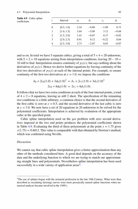
4.3 Polynomial Interpolation 85
Table 4.9 Cubic splinecoefficients i Interval ai bi ci di
0 [0.5,1.0] 2.24 −0.88 −1.09 0.73
1 [1.0,1.5] 3.64 −5.09 3.12 −0.68
2 [1.5,2.0] 1.43 −0.67 0.17 −0.02
3 [2.0,2.5] 0.91 0.12 −0.22 0.04
4 [2.5,3.0] 2.73 −2.07 0.65 −0.07
and so on. In total we have 5 separate cubics, giving a total of 5×4 = 20 unknowns,with 5 × 2 = 10 equations arising from interpolation conditions, leaving 20 − 10 =10 still to find. Interpolation ensures continuity of p3(x), but says nothing about thederivatives of p3(x). Hence we derive further equations by forcing continuity of thefirst two derivatives of p3(x) at each of the internal points. For example, to ensurecontinuity of the first two derivatives at x = 1.0, we impose the conditions
b0 + 2c0(1.0) + 3d0(1.0)2 = b1 + 2c1(1.0) + 3d1(1.0)2
2c0 + 6d0(1.0) = 2c1 + 6d1(1.0).
It follows that we have two extra conditions at each of the four internal points, a totalof 4 × 2 = 8 equations, leaving us still 2 short. The specification of the remainingtwo conditions is a little arbitrary; a common choice is that the second derivative ofthe first cubic is zero at x = 0.5, and the second derivative of the last cubic is zeroat x = 3.0. We now have a set of 20 equations in 20 unknowns to be solved for thepolynomial coefficients. Interpolation is achieved by evaluation of the appropriatecubic at the specified point.
Cubic spline interpolation used on the gas problem with zero second deriva-tives imposed at the two end points produces the polynomial coefficients shownin Table 4.9. Evaluating the third of these polynomials at the point x = 1.75 givesy(1.75) = 0.6812. This value is comparable with that obtained by Newton’s method,which was confirmed using Neville.
Discussion
We cannot say that cubic spline interpolation gives a better approximation than anyother of the methods considered here. A good deal depends on the accuracy of thedata and the underlying function to which we are trying to match our approximat-ing straight lines and polynomials. Nevertheless spline interpolation has been usedsuccessfully in a wide variety of application areas4.
4The use of splines began with the actuarial profession in the late 19th Century. What were thendescribed as osculating (kissing) curves were more prosaically named spline functions when nu-merical analysts became involved in the 1940’s.
86 4 Curve Fitting
4.4 Least Squares Approximation
The final form of approximation we consider has little in common with what hasgone before. The distinguishing feature here is that the straight line, or polynomial,or whatever other form we choose, may not pass through any of the data points,let alone all of them. The use of such an approximation is particularly appropriatewhen it is known that there may be significant errors in the data; to force a curveexactly through the data when it is known that the data is inexact clearly does notmake much sense. Further, we can keep the order of the polynomial low even whenthe number of data points is high, which as we observed in the previous section wasdesirable.
4.4.1 Least Squares Straight Line Approximation
Returning yet again to the gas problem, if we try to construct a straight line p1 =a + bx which exactly fits all the data we have the following system of equations
a + b(0.5) = 1.62
a + b(1.0) = 1.00
a + b(1.5) = 0.75
a + b(2.0) = 0.62
a + b(2.5) = 0.52
a + b(3.0) = 0.46.
This is an overdetermined system of equations in that we have more equations thanunknowns. Since we cannot satisfy all of the equations at once we compromise andlook for a solution in which all of the equations are satisfied approximately. One wayof ensuring this is to minimise the sum of the squares of the differences (or residu-als) between supplied values of the dependent variable (the y-values) and the valuespredicted by the approximation. Although other definitions of what constitutes agood fit are possible, the least squares approximation has some useful mathematicalproperties which makes it relatively easy to compute.
Problem
Fit a least squares straight line to the data of the gas problem. In particular estimatey(1.75).
Solution
We find values of a and b such that

4.4 Least Squares Approximation 87
S(a, b) = (a + b(0.5) − 1.62)2
+ (a + b(1.0) − 1.00)2
+ (a + b(1.5) − 0.75)2
+ (a + b(2.0) − 0.62)2
+ (a + b(2.5) − 0.52)2
+ (a + b(3.0) − 0.46)2
is made as small as possible.Partial derivatives of S with respect to a and b must be zero for a local minimum
and so we have
∂S(a, b)/∂a = 2(a + b(0.5) − 1.62)
+ 2(a + b(1.0) − 1.00)
+ 2(a + b(1.5) − 0.75)
+ 2(a + b(2.0) − 0.62)
+ 2(a + b(2.5) − 0.52)
+ 2(a + b(3.0) − 0.46) = 0
and ∂S(a, b)/∂b = 2(0.5)(a + b(0.5) − 1.62)
+ 2(1.0)(a + b(1.0) − 1.00)
+ 2(1.5)(a + b(1.5) − 0.75)
+ 2(2.0)(a + b(2.0) − 0.62)
+ 2(2.5)(a + b(2.5) − 0.52)
+ 2(3.0)(a + b(3.0) − 0.46) = 0.
From the two equations we have
6a + 10.5b = 4.97 (4.11)
10.5a + 22.75b = 6.855. (4.12)
This set of two equations in two unknowns has a solution a = 1.565333 and b =−0.421143, and so the approximating straight line is y = 1.565333 − 0.421143x
(see Fig. 4.4).
Discussion
Equations (4.11) and (4.12) may be written in the form
an + bSx = Sy (4.13)
aSx + bSxx = Sxy (4.14)
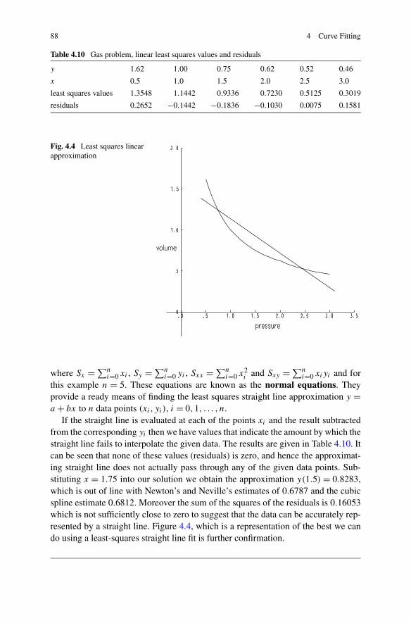
88 4 Curve Fitting
Table 4.10 Gas problem, linear least squares values and residuals
y 1.62 1.00 0.75 0.62 0.52 0.46
x 0.5 1.0 1.5 2.0 2.5 3.0
least squares values 1.3548 1.1442 0.9336 0.7230 0.5125 0.3019
residuals 0.2652 −0.1442 −0.1836 −0.1030 0.0075 0.1581
Fig. 4.4 Least squares linearapproximation
where Sx = ∑ni=0 xi , Sy = ∑n
i=0 yi , Sxx = ∑ni=0 x2
i and Sxy = ∑ni=0 xiyi and for
this example n = 5. These equations are known as the normal equations. Theyprovide a ready means of finding the least squares straight line approximation y =a + bx to n data points (xi, yi), i = 0,1, . . . , n.
If the straight line is evaluated at each of the points xi and the result subtractedfrom the corresponding yi then we have values that indicate the amount by which thestraight line fails to interpolate the given data. The results are given in Table 4.10. Itcan be seen that none of these values (residuals) is zero, and hence the approximat-ing straight line does not actually pass through any of the given data points. Sub-stituting x = 1.75 into our solution we obtain the approximation y(1.5) = 0.8283,which is out of line with Newton’s and Neville’s estimates of 0.6787 and the cubicspline estimate 0.6812. Moreover the sum of the squares of the residuals is 0.16053which is not sufficiently close to zero to suggest that the data can be accurately rep-resented by a straight line. Figure 4.4, which is a representation of the best we cando using a least-squares straight line fit is further confirmation.
4.4 Least Squares Approximation 89
4.4.2 Least Squares Polynomial Approximation
To generalise our discussion of least squares approximation we consider the poly-nomial approximation pm(x), of degree m, which we wish to fit to the n + 1 datapoints (xi, yi). We assume that n is larger than m.
We cannot hope to satisfy (4.15) exactly, so as with the straight line approxima-tion we aim to minimise the sum of squares of residuals.
pm(xi) = yi, i = 0,1, . . . , n (4.15)
where
pm(x) = α0 + α1x + α2x2 + · · · + αmxm. (4.16)
We choose the αi so that S(α ) = ∑ni=0 r2
i , where ri = pm(xi) − yi , is a minimum,which means we must have
∂S(α )
∂αi
= 0, i = 0,1, . . . ,m.
Problem
Fit a least squares quadratic to the data of the gas problem.In particular estimatey(1.75).
Solution
We look for a polynomial p2(x) = α0 +α1x +α2x2 where α0, α1 and α2 are chosen
so that∑5
i=0 (α0 + α1xi + α2x2i − yi)
2is a minimum. Differentiating with respect
to α0, α1 and α2 gives the three equations
5∑
i=0
(α0 + α1xi + α2x
2i
) = 0 (4.17)
5∑
i=0
xi
(α0 + α1xi + α2x
2i
) = 0 (4.18)
5∑
i=0
x2i
(α0 + α1xi + α2x
2i
) = 0. (4.19)
Inserting values for xi and gathering coefficients leads to a 3 × 3 symmetric systemof linear equations, namely
6.0α0 + 10.5α1 + 22.75α2 = 4.97 (4.20)
10.5α0 + 22.75α1 + 55.125α2 = 6.855 (4.21)
22.75α0 + 55.125α1 + 142.1875α2 = 12.9625. (4.22)
90 4 Curve Fitting
Gaussian elimination gives the solution α0 = 2.1320, α1 = −1.2711 and α2 =0.2429 and so the approximating quadratic is 2.1320 − 1.2711x + 0.2429x2.
Equations (4.20)–(4.22) are the normal equations for least squares quadratic ap-proximation. Extending the notation used for the linear case ((4.13) and (4.14)) wemay write
α0n +α1Sx +α2Sxx = Sy
α0Sx +α1Sxx +α2Sxxx = Sxy
α0Sxx +α1Sxxx +α2Sxxxx = Sxxy.
The pattern extends to higher order polynomials, but generally normal equations arewritten in the form
XT Xc = XT y
which for the example above would be
X =
⎛
⎜⎜⎜⎝
1 x0 x20
1 x1 x21
...
1 x5 x25
⎞
⎟⎟⎟⎠
, c =⎛
⎝α0α1α2
⎞
⎠ , y =
⎛
⎜⎜⎜⎝
y0y1...
y5
⎞
⎟⎟⎟⎠
with data values x0 = 0.5, x1 = 1, . . . , x5 = 3.0, y0 = 1.62, y1 = 1, . . . , y5 = 0.46.
Discussion
The residuals for this approximation are shown in Table 4.11. As might be expectedin nearly all cases there is an improvement over linear approximation (Table 4.10).Substituting x = 1.75 in the approximating quadratic we obtain the approximationy(1.75) = 0.6512. This value is an improvement on the linear least squares esti-mate of 0.8283 but still not quite in agreement with earlier estimates obtained usingNewton’s method, Neville interpolation and a cubic spline (0.678965, 0.678672,and 0.6812 respectively). The sum of the squares of residuals has been reducedfrom 0.16053 to 0.229. A least squares cubic polynomial may or may not obtainbetter accuracy but there is a limit as to how far the degree may be raised before themethod becomes unstable and possibly produces an approximating function whichoscillates wildly between the data points. Such a function could not be consideredas being representative of the underlying function. In the case of the gas problem itmay be that a least squares fit based on a function other than a polynomial is moreappropriate. Such a function may be found by investigating the theory underlyingthe relation between gas and pressure or by trial and error. Approximation using the
Table 4.11 Gas problem, quadratic least squares values and residuals
y 1.62 1.00 0.75 0.62 0.52 0.46
x 0.5 1.0 1.5 2.0 2.5 3.0
quadratic least squares values 1.5571 1.1037 0.7717 0.5611 0.4720 0.5043
residuals 0.0629 −0.1037 −0.0217 0.0589 0.0480 −0.0443
4.4 Least Squares Approximation 91
least squares method is not restricted to straight lines or polynomials. Exercise 7 isone such example. The least squares method can also be used in fitting spline curvesto what may be inaccurate data. In order to produce a smoothing effect we allow ap-proximate but controlled interpolation by minimising least squares differences inhigher derivatives where the spline curves meet.
Summary In this chapter we have looked at the approximation of a set of datapoints using a polynomial. There are two distinct possibilities here:
• determine (an explicit or implicit expression for) a polynomial that passes throughall the data points (interpolation).
• determine a polynomial that may not pass through any of the data points but insome sense is a best fit.
Polynomial interpolation can conveniently be further subdivided into
• determine a polynomial interpolant with all derivatives continuous.• determine a polynomial interpolant with only some derivatives continuous.
We have also indicated that polynomials are not the only choice. The least squaresmethod may be used in conjunction with other functions. Where possible the choiceshould be guided by an understanding of the underlying model.
Exercises
1. Table 4.12 gives observed values of Young’s modulus measured at various tem-peratures for a particular stainless steel. Use the code as part of a larger programto verify the values in Table 4.13, which show that the relation between Temper-ature and Young’s modulus is near enough linear for practical purposes.
T = [0:100:600]Y = [ 200 190 185 178 170 160 150]% loop to find first differencesfor i = 1 : 6
diff1(i) = (Y(i+1) − Y(i))/100; % store the first differences in diff1end;diff1% loop to find the second differences
Establish the normal equations for finding the coefficients a and b in the leastsquares straight line approximation
Y = a + bT
Table 4.12 Young’s Modulus in relation to temperature
T : Temperature (Centigrade) 0 100 200 300 400 500 600
Y : Young’s modulus ×10−3 200 190 185 178 170 160 150
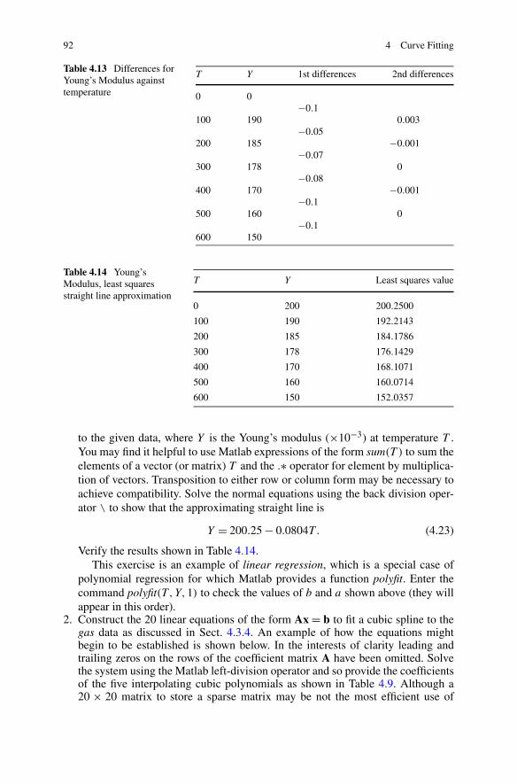
92 4 Curve Fitting
Table 4.13 Differences forYoung’s Modulus againsttemperature
T Y 1st differences 2nd differences
0 0−0.1
100 190 0.003−0.05
200 185 −0.001−0.07
300 178 0−0.08
400 170 −0.001−0.1
500 160 0−0.1
600 150
Table 4.14 Young’sModulus, least squaresstraight line approximation
T Y Least squares value
0 200 200.2500
100 190 192.2143
200 185 184.1786
300 178 176.1429
400 170 168.1071
500 160 160.0714
600 150 152.0357
to the given data, where Y is the Young’s modulus (×10−3) at temperature T .You may find it helpful to use Matlab expressions of the form sum(T ) to sum theelements of a vector (or matrix) T and the .∗ operator for element by multiplica-tion of vectors. Transposition to either row or column form may be necessary toachieve compatibility. Solve the normal equations using the back division oper-ator \ to show that the approximating straight line is
Y = 200.25 − 0.0804T . (4.23)
Verify the results shown in Table 4.14.This exercise is an example of linear regression, which is a special case of
polynomial regression for which Matlab provides a function polyfit. Enter thecommand polyfit(T ,Y,1) to check the values of b and a shown above (they willappear in this order).
2. Construct the 20 linear equations of the form Ax = b to fit a cubic spline to thegas data as discussed in Sect. 4.3.4. An example of how the equations mightbegin to be established is shown below. In the interests of clarity leading andtrailing zeros on the rows of the coefficient matrix A have been omitted. Solvethe system using the Matlab left-division operator and so provide the coefficientsof the five interpolating cubic polynomials as shown in Table 4.9. Although a20 × 20 matrix to store a sparse matrix may be not the most efficient use of
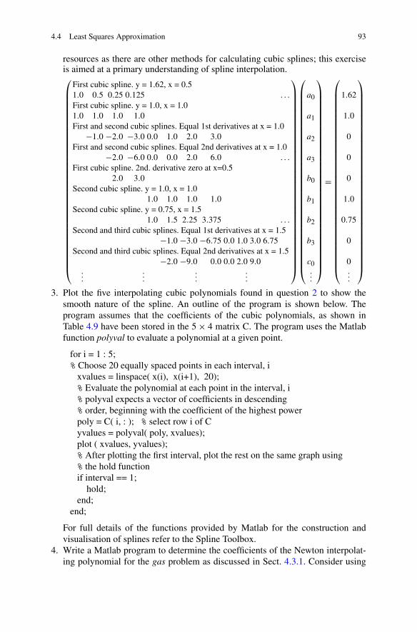
4.4 Least Squares Approximation 93
resources as there are other methods for calculating cubic splines; this exerciseis aimed at a primary understanding of spline interpolation.⎛
⎜⎜⎜⎜⎜⎜⎜⎜⎜⎜⎜⎜⎜⎜⎜⎜⎜⎜⎜⎜⎜⎜⎜⎜⎜⎜⎜⎜⎜⎜⎜⎜⎜⎜⎝
First cubic spline. y = 1.62, x = 0.51.0 0.5 0.25 0.125 . . .
First cubic spline. y = 1.0, x = 1.01.0 1.0 1.0 1.0First and second cubic splines. Equal 1st derivatives at x = 1.0
−1.0 −2.0 −3.0 0.0 1.0 2.0 3.0First and second cubic splines. Equal 2nd derivatives at x = 1.0
−2.0 −6.0 0.0 0.0 2.0 6.0 . . .
First cubic spline. 2nd. derivative zero at x=0.52.0 3.0
Second cubic spline. y = 1.0, x = 1.01.0 1.0 1.0 1.0
Second cubic spline. y = 0.75, x = 1.51.0 1.5 2.25 3.375 . . .
Second and third cubic splines. Equal 1st derivatives at x = 1.5−1.0 −3.0 −6.75 0.0 1.0 3.0 6.75
Second and third cubic splines. Equal 2nd derivatives at x = 1.5−2.0 −9.0 0.0 0.0 2.0 9.0
......
......
⎞
⎟⎟⎟⎟⎟⎟⎟⎟⎟⎟⎟⎟⎟⎟⎟⎟⎟⎟⎟⎟⎟⎟⎟⎟⎟⎟⎟⎟⎟⎟⎟⎟⎟⎟⎠
⎛
⎜⎜⎜⎜⎜⎜⎜⎜⎜⎜⎜⎜⎜⎜⎜⎜⎜⎜⎜⎜⎜⎜⎜⎜⎜⎜⎜⎜⎜⎜⎜⎜⎜⎜⎝
a0
a1
a2
a3
b0
b1
b2
b3
c0...
⎞
⎟⎟⎟⎟⎟⎟⎟⎟⎟⎟⎟⎟⎟⎟⎟⎟⎟⎟⎟⎟⎟⎟⎟⎟⎟⎟⎟⎟⎟⎟⎟⎟⎟⎟⎠
=
⎛
⎜⎜⎜⎜⎜⎜⎜⎜⎜⎜⎜⎜⎜⎜⎜⎜⎜⎜⎜⎜⎜⎜⎜⎜⎜⎜⎜⎜⎜⎜⎜⎜⎜⎜⎝
1.62
1.0
0
0
0
1.0
0.75
0
0...
⎞
⎟⎟⎟⎟⎟⎟⎟⎟⎟⎟⎟⎟⎟⎟⎟⎟⎟⎟⎟⎟⎟⎟⎟⎟⎟⎟⎟⎟⎟⎟⎟⎟⎟⎟⎠
3. Plot the five interpolating cubic polynomials found in question 2 to show thesmooth nature of the spline. An outline of the program is shown below. Theprogram assumes that the coefficients of the cubic polynomials, as shown inTable 4.9 have been stored in the 5 × 4 matrix C. The program uses the Matlabfunction polyval to evaluate a polynomial at a given point.
for i = 1 : 5;% Choose 20 equally spaced points in each interval, i
xvalues = linspace( x(i), x(i+1), 20);% Evaluate the polynomial at each point in the interval, i% polyval expects a vector of coefficients in descending% order, beginning with the coefficient of the highest powerpoly = C( i, : ); % select row i of Cyvalues = polyval( poly, xvalues);plot ( xvalues, yvalues);% After plotting the first interval, plot the rest on the same graph using% the hold functionif interval == 1;
hold;end;
end;
For full details of the functions provided by Matlab for the construction andvisualisation of splines refer to the Spline Toolbox.
4. Write a Matlab program to determine the coefficients of the Newton interpolat-ing polynomial for the gas problem as discussed in Sect. 4.3.1. Consider using
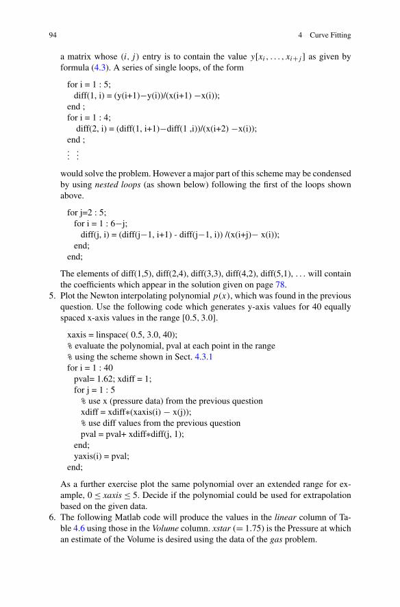
94 4 Curve Fitting
a matrix whose (i, j) entry is to contain the value y[xi, . . . , xi+j ] as given byformula (4.3). A series of single loops, of the form
for i = 1 : 5;diff(1, i) = (y(i+1)−y(i))/(x(i+1) −x(i));
end ;for i = 1 : 4;
diff(2, i) = (diff(1, i+1)−diff(1 ,i))/(x(i+2) −x(i));end ;...
...
would solve the problem. However a major part of this scheme may be condensedby using nested loops (as shown below) following the first of the loops shownabove.
for j=2 : 5;for i = 1 : 6−j;
diff(j, i) = (diff(j−1, i+1) - diff(j−1, i)) /(x(i+j)− x(i));end;
end;
The elements of diff(1,5), diff(2,4), diff(3,3), diff(4,2), diff(5,1), . . . will containthe coefficients which appear in the solution given on page 78.
5. Plot the Newton interpolating polynomial p(x), which was found in the previousquestion. Use the following code which generates y-axis values for 40 equallyspaced x-axis values in the range [0.5,3.0].
xaxis = linspace( 0.5, 3.0, 40);% evaluate the polynomial, pval at each point in the range% using the scheme shown in Sect. 4.3.1for i = 1 : 40
pval= 1.62; xdiff = 1;for j = 1 : 5% use x (pressure data) from the previous questionxdiff = xdiff∗(xaxis(i) − x(j));% use diff values from the previous questionpval = pval+ xdiff∗diff(j, 1);
end;yaxis(i) = pval;
end;
As a further exercise plot the same polynomial over an extended range for ex-ample, 0 ≤ xaxis ≤ 5. Decide if the polynomial could be used for extrapolationbased on the given data.
6. The following Matlab code will produce the values in the linear column of Ta-ble 4.6 using those in the Volume column. xstar (= 1.75) is the Pressure at whichan estimate of the Volume is desired using the data of the gas problem.
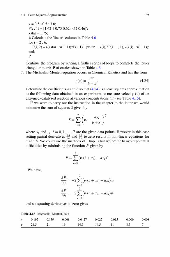
4.4 Least Squares Approximation 95
x = 0.5 : 0.5 : 3.0;P(: , 1) = [1.62 1 0.75 0.62 0.52 0.46]';xstar = 1.75;% Calculate the 'linear' column in Table 4.6for i = 2 : 6;
P(i, 2) = ((xstar−x(i−1))*P(i, 1)−(xstar − x(i))*P(i−1, 1)) /(x(i)−x(i−1));end;P
Continue the program by writing a further series of loops to complete the lowertriangular matrix P of entries shown in Table 4.6.
7. The Michaelis–Menten equation occurs in Chemical Kinetics and has the form
v(x) = ax
b + x. (4.24)
Determine the coefficients a and b so that (4.24) is a least squares approximationto the following data obtained in an experiment to measure velocity (v) of anenzymed–catalysed reaction at various concentrations (x) (see Table 4.15).
If we were to carry out the instruction in the chapter to the letter we wouldminimise the sum of squares S given by
S =7∑
i=0
(
vi − axi
b + xi
)2
where xi and vi , i = 0,1, . . . ,7 are the given data points. However in this casesetting partial derivatives ∂S
∂aand ∂S
∂bto zero results in non-linear equations for
a and b. We could use the methods of Chap. 3 but we prefer to avoid potentialdifficulties by minimising the function P given by
P =7∑
i=0
(vi(b + xi) − axi
)2.
We have
∂P
∂a= −2
7∑
i=0
(vi(b + xi) − axi
)xi
∂P
∂b= 2
7∑
i=0
(vi(b + xi) − axi
)vi
and so equating derivatives to zero gives
Table 4.15 Michaelis–Menten, data
x 0.197 0.139 0.068 0.0427 0.027 0.015 0.009 0.008
v 21.5 21 19 16.5 14.5 11 8.5 7
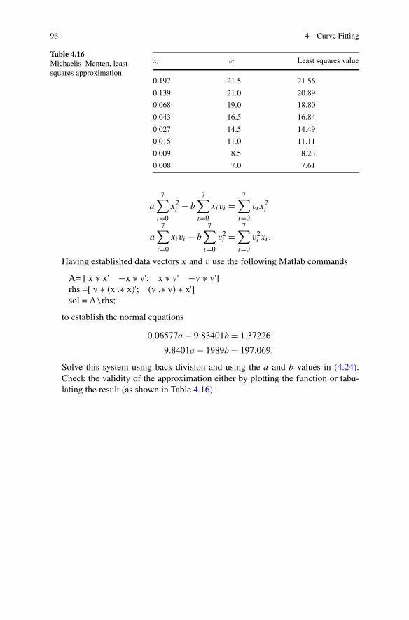
96 4 Curve Fitting
Table 4.16Michaelis–Menten, leastsquares approximation
xi vi Least squares value
0.197 21.5 21.56
0.139 21.0 20.89
0.068 19.0 18.80
0.043 16.5 16.84
0.027 14.5 14.49
0.015 11.0 11.11
0.009 8.5 8.23
0.008 7.0 7.61
a
7∑
i=0
x2i − b
7∑
i=0
xivi =7∑
i=0
vix2i
a
7∑
i=0
xivi − b
7∑
i=0
v2i =
7∑
i=0
v2i xi .
Having established data vectors x and v use the following Matlab commands
A= [ x ∗ x' −x ∗ v'; x ∗ v' −v ∗ v']rhs =[ v ∗ (x .∗ x)'; (v .∗ v) ∗ x']sol = A\rhs;
to establish the normal equations
0.06577a − 9.83401b = 1.37226
9.8401a − 1989b = 197.069.
Solve this system using back-division and using the a and b values in (4.24).Check the validity of the approximation either by plotting the function or tabu-lating the result (as shown in Table 4.16).
Chapter 5Numerical Integration
Aims In this chapter we look at ways of calculating an approximation to a def-inite integral of a real-valued function of a single variable, f (x) (the integrand).Sometimes integration can be achieved using standard formulae, possibly after somemanipulation to express the integral in a particular form. However, often standardformulae cannot be used (for example, the function may be known at a discrete setof points only) and so it is necessary to resort to numerical techniques. The pointsat which the integrand is to be evaluated are known as grid points or mesh points,although the terms data points or just points may also be used. The terms grid ormesh are equivalent and generally refer to a collection or division of an interval intogrid points or mesh points.
Overview All the methods that we look at involve approximating an integral witha weighted sum of evaluations of the integrand. The methods differ in some or allof the following aspects:
• the spacing of the points at which the integrand is evaluated.• the weights associated with the function evaluations.• the accuracy that a method achieves for a given number of function evaluations.• the convergence characteristics of the method (how the approximation improves
with the addition of new function values).
In particular we look at
• the trapezium rule.• Simpson’s rule.• Newton–Cotes rules.• Gaussian quadrature.• adaptive quadrature.
Acquired Skills After reading this chapter you will be able to estimate values ofdefinite integrals of a wide range of functions. Although the methods which you willhave at your disposal will give an approximate result, you will nevertheless be ableto judge the level of accuracy. Furthermore, you will be able to make an informedchoice of method to use in any given application.
C. Woodford, C. Phillips, Numerical Methods with Worked Examples: Matlab Edition,DOI 10.1007/978-94-007-1366-6_5, © Springer Science+Business Media B.V. 2012
97
98 5 Numerical Integration
5.1 Introduction
A number of standard formulae are available for evaluating, analytically, definiteintegrals. A particular example is provided by
∫ b
a
xk dx =[
xk+1
k + 1
]b
a
= 1
k + 1
[bk+1 − ak+1]
so that, for example,∫ 1
0 x dx = 12 . In addition, there are a number of standard tech-
niques for manipulating an integral so that it matches one of these formulae. Aparticular case in point is the technique of integration by parts:
∫ b
a
u(x)dv(x)
dxdx = [
u(x)v(x)]ba−
∫ b
a
v(x)du(x)
dxdx
which can be used, for example, to derive the result∫ 1
0xex dx = xex
∣∣10−
∫ 1
0ex dx = e − e + 1 = 1.
However, practical problems often involve an integrand (the function to be in-tegrated) for which there is no known analytic form. The integral
∫e−t2
dt is anexample. On the other hand integrals may arise which involve an integrand requir-ing considerable effort to reduce to standard form and so a numerical approximationmay be more practical. Other practical problems involve integrands for which val-ues are only available at a number of discrete points. In this chapter we look at waysof dealing with all such problems. The first group of methods we investigate areknown as the Newton–Cotes rules and include the trapezium rule, Simpson’s ruleand higher order rules, based on evaluating the integrand at equally-spaced points.If there is no restriction on the points at which the integrand may be evaluated, thenother methods such as Gaussian quadrature may be more suitable.
5.2 Integration of Tabulated Functions
To illustrate the methods for dealing with functions for which values are only avail-able at a number of points we consider the following problem.
Problem
A company has a contract to build a ship, the cost of which will be a function of,amongst other things, the surface area of the deck. The deck is symmetric abouta line drawn from the tip of the bow to the tip of the stern (Fig. 5.1) and so itis sufficient to determine the area of one half of the deck and then to double theresult. The ship is 235 metres long. Table 5.1 gives half-breadths (distances fromthe middle of the deck to the edge) at various grid points along the centre line, asmeasured from a draughtsman’s drawing of the proposed vessel. Grid points are
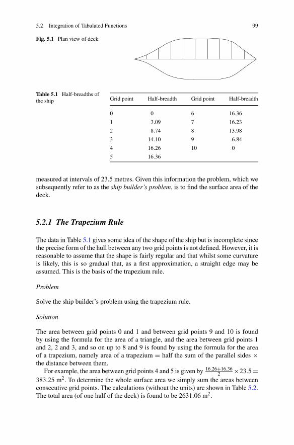
5.2 Integration of Tabulated Functions 99
Fig. 5.1 Plan view of deck
Table 5.1 Half-breadths ofthe ship Grid point Half-breadth Grid point Half-breadth
0 0 6 16.36
1 3.09 7 16.23
2 8.74 8 13.98
3 14.10 9 6.84
4 16.26 10 0
5 16.36
measured at intervals of 23.5 metres. Given this information the problem, which wesubsequently refer to as the ship builder’s problem, is to find the surface area of thedeck.
5.2.1 The Trapezium Rule
The data in Table 5.1 gives some idea of the shape of the ship but is incomplete sincethe precise form of the hull between any two grid points is not defined. However, it isreasonable to assume that the shape is fairly regular and that whilst some curvatureis likely, this is so gradual that, as a first approximation, a straight edge may beassumed. This is the basis of the trapezium rule.
Problem
Solve the ship builder’s problem using the trapezium rule.
Solution
The area between grid points 0 and 1 and between grid points 9 and 10 is foundby using the formula for the area of a triangle, and the area between grid points 1and 2, 2 and 3, and so on up to 8 and 9 is found by using the formula for the areaof a trapezium, namely area of a trapezium = half the sum of the parallel sides ×the distance between them.
For example, the area between grid points 4 and 5 is given by 16.26+16.362 ×23.5 =
383.25 m2. To determine the whole surface area we simply sum the areas betweenconsecutive grid points. The calculations (without the units) are shown in Table 5.2.The total area (of one half of the deck) is found to be 2631.06 m2.
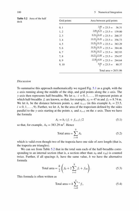
100 5 Numerical Integration
Table 5.2 Area of the halfdeck Grid points Area between grid points
0, 1 3.092 × 23.5 = 36.31
1, 2 3.09+8.742 × 23.5 = 139.00
2, 3 8.74+14.102 × 23.5 = 268.37
3, 4 14.10+16.262 × 23.5 = 356.73
4, 5 16.26+16.362 × 23.5 = 383.29
5, 6 16.36+16.362 × 23.5 = 384.46
6, 7 16.36+16.232 × 23.5 = 382.93
7, 8 16.23+13.982 × 23.5 = 354.97
8, 9 13.98+6.842 × 23.5 = 244.64
9, 10 6.842 × 23.5 = 80.37
Total area = 2631.06
Discussion
To summarise this approach mathematically we regard Fig. 5.1 as a graph, with thex-axis running along the middle of the ship, and grid points along the x-axis. They-axis then represents half-breadths. We let xi : i = 0,1, . . . ,10 represent points atwhich half-breadths fi are known, so that, for example, x2 = 47 m and f2 = 8.74 m.We let hi be the distance between points xi and xi+1 (in this example hi = 23.5,i = 0,1, . . . ,9). Further, we let Ai be the area of the trapezium defined by the sidesparallel to the y-axis starting at the points xi and xi+1 on the x-axis. Then we havethe formula
Ai = hi (fi + fi+1) /2 (5.1)
so that, for example, A4 = 383.29 m2. Hence
Total area =9∑
i=0
Ai (5.2)
which is valid even though two of the trapezia have one side of zero length (that is,the trapezia are triangles).
We can see from Table 5.2 that in the total sum each of the half-breadths corre-sponding to an internal section (that is, a section other than x0 and x10) is countedtwice. Further, if all spacings hi have the same value, h we have the alternativeformula
Total area = h
2
(f0 + 2
9∑i=1
fi + f10
). (5.3)
This formula is often written as
Total area = h
n∑i=0
′′fi, (5.4)
5.2 Integration of Tabulated Functions 101
where the double prime on the summation sign means that the first and last termsare to be halved.
5.2.2 Quadrature Rules
In the example above the triangles and trapezia are known as panels. Formulas suchas (5.1) which are based on the areas of panels are known as quadrature rules.When a quadrature rule is derived by combining several simple rules, as in (5.2),(5.3) or (5.4), we refer to a composite (quadrature) rule. In general, a compositerule based on n + 1 points takes the form
Total area =n∑
i=0
wifi. (5.5)
We refer to such rules, which are a linear combination of a set of observations fi
in which the wi are the weights, as n-point (counting from zero), or n-panel, rules.The two-point rule (5.1) which determines the area of a trapezium is understandablycalled the trapezium rule. For the composite trapezium rule the weights in (5.5) aregiven by w0 = wn = h/2 and wi = h for i �= 0 or n. Note that the term compositetrapezium rule is often abbreviated to trapezium rule.
The first solution to the ship builder’s problem made the assumption that it wassafe to approximate the shape of the hull by straight lines. This seems reasonable,particularly in the middle section, but it is less defensible at the bow and stern.
To improve the situation (without any justification, at the moment) we employ aformula similar to (5.3), but change the weighting. This forms the basis of Simpson’sRule1 which we illustrate in the following problem.
5.2.3 Simpson’s Rule
Problem
Solve the ship builder’s problem using Simpson’s rule.
Solution
This time the end grid points are given a weight of h3 , the odd-numbered internal
grid points are given a weight of 4h3 , whilst the even-numbered internal grid points
1The rule is attributed to Thomas Simpson 1710–1761, mathematician and fellow of the RoyalSociety, but it was in use a hundred years earlier. Known as the Oracle of Nuneaton he was forcedto flee to Derby after dressing up as the Devil.
102 5 Numerical Integration
are given a weight of 2h3 , to give the formula
Total area = h
3
(f0 + 4
5∑i=1
f2i−1 + 24∑
i=1
f2i + f10
). (5.6)
We then have an estimate of the total area of 2641.09 m2, which we suggest is likelyto be more accurate than that given by the trapezium rule.
Discussion
Now for a partial justification of Simpson’s rule (a more comprehensive justificationis given in the next section). In the previous subsection the ten-panel compositerule (5.3) was derived from the one-panel rule (5.1). Similarly, the composite rule(5.6) can be obtained by accumulating a sequence of 5 partial results. We groupthe grid points into sets of 3, to obtain (0,1,2), (2,3,4), and so on. Then for eachgroup we compute an area estimate using the weighting h
3 , 4h3 and h
3 . It is the ratio1 : 4 : 1 which is important; the factor 1
3 is there to ensure that the final calculationis scaled correctly. The ratio 1 : 4 : 1 ensures that the formula is accurate not onlyfor linear functions (which was the case for the trapezium rule) but (as we willsee) also for quadratic and cubic polynomials and so in general is likely to providegreater accuracy. When partial results are combined to form a composite rule theratio becomes 1 : 4 : 2 : · · · : 4 : 2 : 4 : 1, as in (5.6).
5.2.4 Integration from Irregularly-Spaced Data
The rules that we have used so far have been based on the assumption that thedata supplied represents the outline of the hull to a reasonable degree of accuracy.Near the centre of the ship we can expect the shape between grid points to be fairlyflat, and so the trapezium rule estimates based on the information supplied will beadequate. Near the bow and stern we would expect more curvature which, as we willsee later, is something Simpson’s rule attempts to reflect. An alternative approach isto increase the amount of information available in those regions where the curvatureis most pronounced.
Problem
In order that the cost of production can be more accurately determined, the shipbuilding company have supplied additional information in which an extra twoequally spaced points have been introduced between grid points 0 and 1, 1 and 2, 8and 9, and 9 and 10, and mid-points between grid points 2 and 3, 3 and 4, 6 and 7,and 7 and 8. Unfortunately the figures supplied by the ship building company, givenin Table 5.3, failed to include the data for the point 0.25.
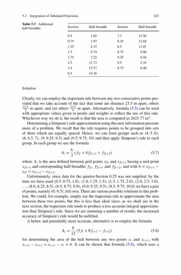
5.2 Integration of Tabulated Functions 103
Table 5.3 Additionalhalf-breadths Section Half-breadth Section Half-breadth
0.5 1.05 7.5 15.56
0.75 1.97 8.25 12.68
1.25 4.33 8.5 11.01
1.5 5.74 8.75 9.06
1.75 7.22 9.25 4.56
2.5 11.73 9.5 2.34
3.5 15.57 9.75 0.40
6.5 16.36
Solution
Clearly, we can employ the trapezium rule between any two consecutive points pro-vided that we take account of the fact that some are distance 23.5 m apart, others23.5
2 m apart, and yet others 23.54 m apart. Alternatively, formula (5.5) can be used
with appropriate values given to points and weights to reflect the use of this rule.Whichever way we do it, the result is that the area is computed as 2625.77 m2.
Determining a Simpson’s rule approximation using this new information presentsmore of a problem. We recall that the rule requires points to be grouped into setsof three which are equally spaced. Hence, we can form groups such as (4,5,6),(6,6.5,7), (9,9.25,9.5) and (9.5,9.75,10) and then apply Simpson’s rule to eachgroup. In each group we use the formula
Ai = h
3(f2i + 4f2i+1 + f2i+2) (5.7)
where Ai is the area defined between grid points x2i and x2i+2 having a mid-pointx2i+1 and corresponding half-breadths f2i , f2i+1 and f2i+2, and with h = x2i+1 −x2i = x2i+2 − x2i+1.
Unfortunately, since data for the quarter-Section 0.25 was not supplied, by thetime we have used (0.5,0.75,1.0), (1.0,1.25,1.5), (1.5,1.75,2.0), (2.0,2.5,3.0),. . ., (8.0,8.25,8.5), (8.5,8.75,9.0), (9.0,9.25,9.5), (9.5,9.75,10.0) we have a pairof points, namely (0,0.5), left over. There are various possible solutions to this prob-lem. We could, for example, simply use the trapezium rule to approximate the areabetween these two points, but this is less than ideal since, as we shall see in thenext section, the trapezium rule tends to produce a less accurate integral approxima-tion than Simpson’s rule. Since we are summing a number of results, the increasedaccuracy of Simpson’s rule would be nullified.
A better, and potentially more accurate, alternative is to employ the formula
Ai = h
12(5fi + 8fi+1 − fi+2) (5.8)
for determining the area of the hull between any two points xi and xi+1, withxi+2 − xi+1 = xi+1 − xi = h. It can be shown that formula (5.8), which uses a
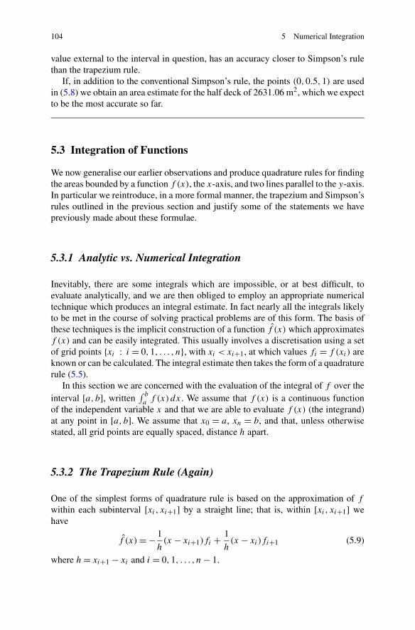
104 5 Numerical Integration
value external to the interval in question, has an accuracy closer to Simpson’s rulethan the trapezium rule.
If, in addition to the conventional Simpson’s rule, the points (0,0.5,1) are usedin (5.8) we obtain an area estimate for the half deck of 2631.06 m2, which we expectto be the most accurate so far.
5.3 Integration of Functions
We now generalise our earlier observations and produce quadrature rules for findingthe areas bounded by a function f (x), the x-axis, and two lines parallel to the y-axis.In particular we reintroduce, in a more formal manner, the trapezium and Simpson’srules outlined in the previous section and justify some of the statements we havepreviously made about these formulae.
5.3.1 Analytic vs. Numerical Integration
Inevitably, there are some integrals which are impossible, or at best difficult, toevaluate analytically, and we are then obliged to employ an appropriate numericaltechnique which produces an integral estimate. In fact nearly all the integrals likelyto be met in the course of solving practical problems are of this form. The basis ofthese techniques is the implicit construction of a function f (x) which approximatesf (x) and can be easily integrated. This usually involves a discretisation using a setof grid points {xi : i = 0,1, . . . , n}, with xi < xi+1, at which values fi = f (xi) areknown or can be calculated. The integral estimate then takes the form of a quadraturerule (5.5).
In this section we are concerned with the evaluation of the integral of f over theinterval [a, b], written
∫ b
af (x) dx. We assume that f (x) is a continuous function
of the independent variable x and that we are able to evaluate f (x) (the integrand)at any point in [a, b]. We assume that x0 = a, xn = b, and that, unless otherwisestated, all grid points are equally spaced, distance h apart.
5.3.2 The Trapezium Rule (Again)
One of the simplest forms of quadrature rule is based on the approximation of f
within each subinterval [xi, xi+1] by a straight line; that is, within [xi, xi+1] wehave
f (x) = − 1
h(x − xi+1)fi + 1
h(x − xi)fi+1 (5.9)
where h = xi+1 − xi and i = 0,1, . . . , n − 1.
5.3 Integration of Functions 105
The fact that f (xi) = fi and f (xi+1) = fi+1 can be readily verified by substitut-ing xi and xi+1 in turn into (5.9). We say that f (x) interpolates f (x) at the pointsxi and xi+1. Because of its straight-line form, f (x) is referred to as the linear inter-polant and the form given here is equivalent to that given by (4.1) of Chap. 4 withf replacing y and x replacing x.
Since x0 = a and xn = b, we have
∫ b
a
f (x) dx =n−1∑i=0
∫ xi+1
xi
f (x) dx.
But ∫ xi+1
xi
f (x) dx
∫ xi+1
xi
f (x) dx
= − 1
h
∫ xi+1
xi
(x − xi+1)fi dx + 1
h
∫ xi+1
xi
(x − xi)fi+1 dx.
Now ∫ xi+1
xi
(x − xi+1)fi dx = fi
∫ 0
−h
x dx = −h2
2fi
and similarly∫ xi+1
xi
(x − xi)fi+1 dx = fi+1
∫ h
0x dx = h2
2fi+1.
Hence we have replaced an integral that, in principle, we were unable to performanalytically by the sum of two integrals which are readily determined analytically.Hence we obtain the approximation∫ xi+1
xi
f (x) dx ≈ h
2(fi + fi+1)
which compares with (5.1).Summing over all the grid points we have
∫ b
a
f (x) dx ≈ h
n∑i=0
′′fi.
It can be shown that if Ii represents the true integral and Ri the approximationover a single panel [xi, xi+1], then the error, Ei = Ii − Ri is given by
Ei = −h3
12f ′′(ηi) (5.10)
where ηi is some (unknown) point between xi and xi+1.The proof depends on writing the difference between f (x) and the linear inter-
polant f (x) as
f (x) − f (x) = (x − xi)(x − xi+1)
2f ′′(ϒ)
106 5 Numerical Integration
where ϒ is some point in [xi, xi+1]. The error of the interpolation, Ei is given by
Ei =∫ xi+1
xi
(x − xi)(x − xi+1)
2f ′′(ϒ)dx.
This integral cannot be evaluated directly since ϒ is a function but we can use thesecond mean value theorem for integrals to show
Ei = f ′′(ηi)
2
∫ xi+1
xi
(x − xi)(x − xi+1) dx
where ηi is in the range [xi, xi+1] and so by carrying out the integration we have(5.10).
For the composite rule R, the error, E = I − R, where I is the true integral over[a, b], consists of the sum of individual one-panel errors of the form (5.10). Thiscan be simplified to
E = −h2
12(b − a)f ′′(η) (5.11)
where η is some point in [a, b]. The result is interesting. The second derivative of astraight line function is zero, but for a quadratic it is non-zero; hence the trapeziumrule integrates a straight line exactly (as we would expect) but not a quadratic. Theother point to note is that since E is proportional to h2 then a reduction in the meshspacing by a factor of 2 (i.e. doubling the number of panels) should, theoretically,reduce the error by a factor of 4 (although this argument only holds for sufficientlysmooth functions).
5.3.3 Simpson’s Rule (Again)
Simpson’s rule follows in a similar way, using approximation by quadratics insteadof approximation by straight lines (cf. Sect. 5.2.3). We expect such an approximationto be more accurate since it allows for a certain amount of curvature. We take an oddnumber of grid points {xi : i = 0,1, . . . ,2n} (and hence even number of panels)with x0 = a and x2n = b.
We require an approximating quadratic f (x) such that f (xj ) = f (xj ) for j =2i,2i +1,2i +2, i = 0,1, . . . , n−1 and for this it is convenient to use the Lagrangeinterpolation formula namely,
f (x) = 1
2h2
((x − x2i+1)(x − x2i+2)f2i − 2(x − x2i )(x − x2i+2)f2i+1
+ (x − x2i )(x − x2i+1)f2i+2)
(5.12)
which is Newton’s interpolating quadratic, (4.5) Chap. 4, in a different form. Wethen make the approximation
5.3 Integration of Functions 107
∫ x2i+2
x2i
f (x) dx ≈∫ x2i+2
x2i
f (x) dx.
To integrate (5.12) we follow the pattern set by our analysis of the trapezium rule.We have ∫ x2i+2
x2i
(x − x2i+1)(x − x2i+2) dx =∫ h
−h
x(x − h)dx
=[x3
3− h
x2
2
]h
−h
= 2h3
3.
Similarly ∫ x2i+2
x2i
(x − x2i )(x − x2i+2) dx = −4h3
3(5.13)
and ∫ x2i+2
x2i
(x − x2i )(x − x2i−1) dx = 2h3
3. (5.14)
Aggregating these results we obtain the approximating rule∫ x2i+2
x2i
f (x) ≈ h
3(f2i + 4f2i+1 + f2i+2) . (5.15)
Summing all approximations of this form we have
∫ b
a
f (x) dx =n−1∑i=0
∫ x2i+2
x2i
f (x) dx
= h
3
(f (a) + 4
n−1∑i=1
f (x2i−1) + 2n−1∑i=1
f (x2i ) + f (b)
).
As with the trapezium rule it is possible to obtain an expression for the error in theSimpson’s integration rule.
We have that for a single application
E = −h5f (iv)(η)
2880(5.16)
and for the composite rule
E = −h4f (iv)(η)
180(b − a) (5.17)
where η is some unknown point between a and b.Since the fourth derivative of a cubic polynomial is identically zero, we have
a rule that despite being constructed to integrate a quadratic, Simpson’s rule willintegrate a cubic exactly.
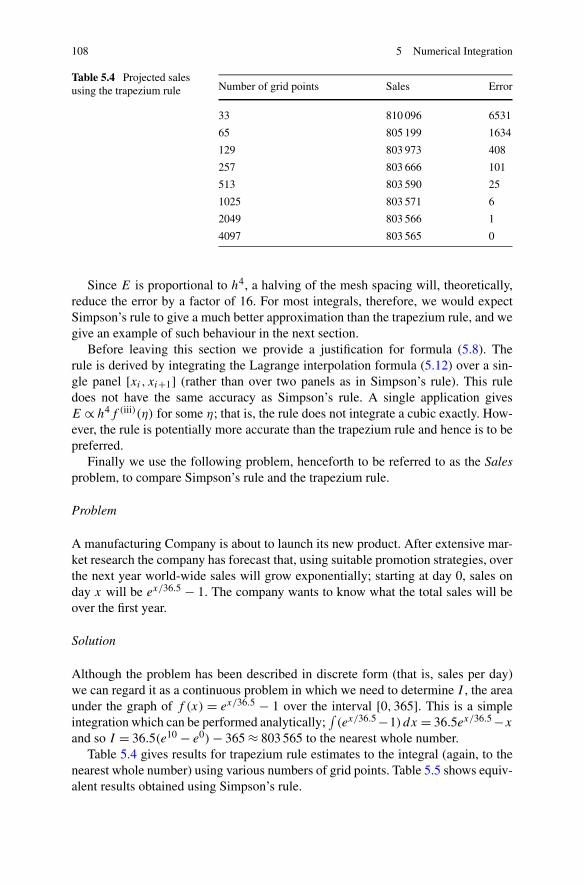
108 5 Numerical Integration
Table 5.4 Projected salesusing the trapezium rule Number of grid points Sales Error
33 810 096 6531
65 805 199 1634
129 803 973 408
257 803 666 101
513 803 590 25
1025 803 571 6
2049 803 566 1
4097 803 565 0
Since E is proportional to h4, a halving of the mesh spacing will, theoretically,reduce the error by a factor of 16. For most integrals, therefore, we would expectSimpson’s rule to give a much better approximation than the trapezium rule, and wegive an example of such behaviour in the next section.
Before leaving this section we provide a justification for formula (5.8). Therule is derived by integrating the Lagrange interpolation formula (5.12) over a sin-gle panel [xi, xi+1] (rather than over two panels as in Simpson’s rule). This ruledoes not have the same accuracy as Simpson’s rule. A single application givesE ∝ h4f (iii)(η) for some η; that is, the rule does not integrate a cubic exactly. How-ever, the rule is potentially more accurate than the trapezium rule and hence is to bepreferred.
Finally we use the following problem, henceforth to be referred to as the Salesproblem, to compare Simpson’s rule and the trapezium rule.
Problem
A manufacturing Company is about to launch its new product. After extensive mar-ket research the company has forecast that, using suitable promotion strategies, overthe next year world-wide sales will grow exponentially; starting at day 0, sales onday x will be ex/36.5 − 1. The company wants to know what the total sales will beover the first year.
Solution
Although the problem has been described in discrete form (that is, sales per day)we can regard it as a continuous problem in which we need to determine I , the areaunder the graph of f (x) = ex/36.5 − 1 over the interval [0,365]. This is a simpleintegration which can be performed analytically;
∫(ex/36.5 −1) dx = 36.5ex/36.5 −x
and so I = 36.5(e10 − e0) − 365 ≈ 803 565 to the nearest whole number.Table 5.4 gives results for trapezium rule estimates to the integral (again, to the
nearest whole number) using various numbers of grid points. Table 5.5 shows equiv-alent results obtained using Simpson’s rule.
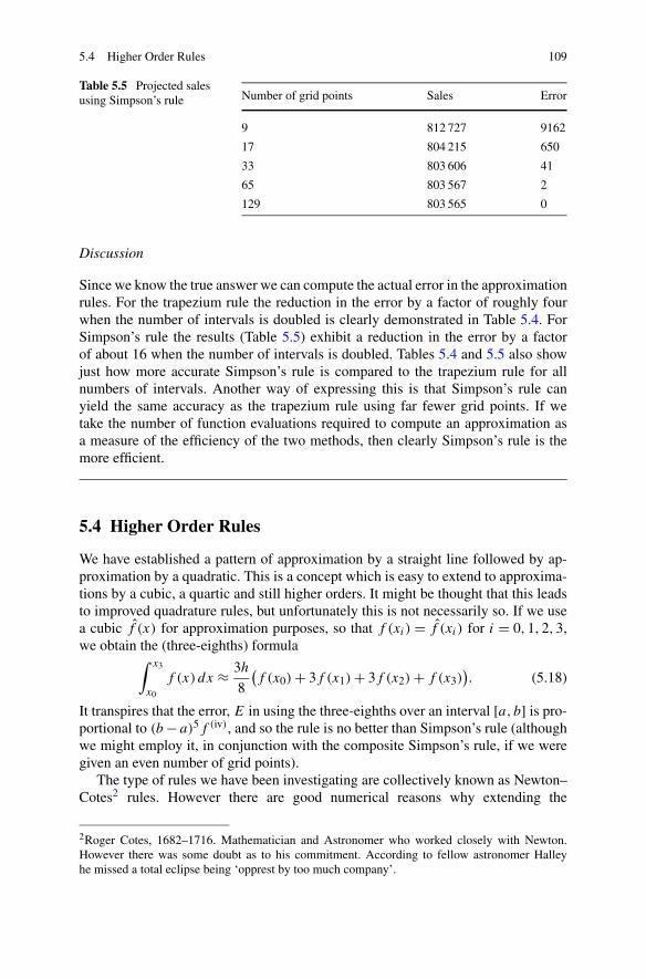
5.4 Higher Order Rules 109
Table 5.5 Projected salesusing Simpson’s rule Number of grid points Sales Error
9 812 727 9162
17 804 215 650
33 803 606 41
65 803 567 2
129 803 565 0
Discussion
Since we know the true answer we can compute the actual error in the approximationrules. For the trapezium rule the reduction in the error by a factor of roughly fourwhen the number of intervals is doubled is clearly demonstrated in Table 5.4. ForSimpson’s rule the results (Table 5.5) exhibit a reduction in the error by a factorof about 16 when the number of intervals is doubled. Tables 5.4 and 5.5 also showjust how more accurate Simpson’s rule is compared to the trapezium rule for allnumbers of intervals. Another way of expressing this is that Simpson’s rule canyield the same accuracy as the trapezium rule using far fewer grid points. If wetake the number of function evaluations required to compute an approximation asa measure of the efficiency of the two methods, then clearly Simpson’s rule is themore efficient.
5.4 Higher Order Rules
We have established a pattern of approximation by a straight line followed by ap-proximation by a quadratic. This is a concept which is easy to extend to approxima-tions by a cubic, a quartic and still higher orders. It might be thought that this leadsto improved quadrature rules, but unfortunately this is not necessarily so. If we usea cubic f (x) for approximation purposes, so that f (xi) = f (xi) for i = 0,1,2,3,we obtain the (three-eighths) formula∫ x3
x0
f (x)dx ≈ 3h
8
(f (x0) + 3f (x1) + 3f (x2) + f (x3)
). (5.18)
It transpires that the error, E in using the three-eighths over an interval [a, b] is pro-portional to (b − a)5f (iv), and so the rule is no better than Simpson’s rule (althoughwe might employ it, in conjunction with the composite Simpson’s rule, if we weregiven an even number of grid points).
The type of rules we have been investigating are collectively known as Newton–Cotes2 rules. However there are good numerical reasons why extending the
2Roger Cotes, 1682–1716. Mathematician and Astronomer who worked closely with Newton.However there was some doubt as to his commitment. According to fellow astronomer Halleyhe missed a total eclipse being ‘opprest by too much company’.
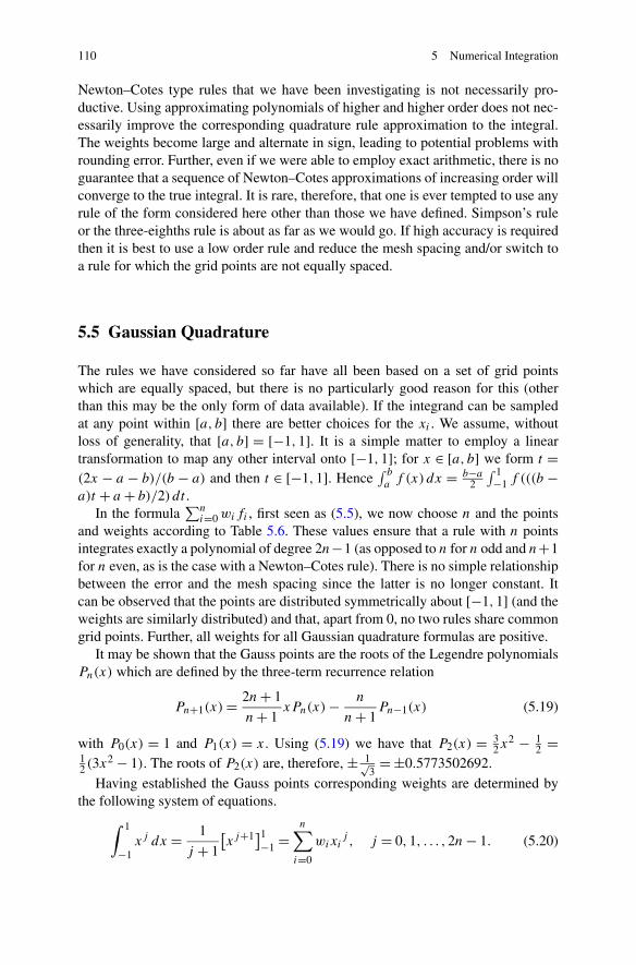
110 5 Numerical Integration
Newton–Cotes type rules that we have been investigating is not necessarily pro-ductive. Using approximating polynomials of higher and higher order does not nec-essarily improve the corresponding quadrature rule approximation to the integral.The weights become large and alternate in sign, leading to potential problems withrounding error. Further, even if we were able to employ exact arithmetic, there is noguarantee that a sequence of Newton–Cotes approximations of increasing order willconverge to the true integral. It is rare, therefore, that one is ever tempted to use anyrule of the form considered here other than those we have defined. Simpson’s ruleor the three-eighths rule is about as far as we would go. If high accuracy is requiredthen it is best to use a low order rule and reduce the mesh spacing and/or switch toa rule for which the grid points are not equally spaced.
5.5 Gaussian Quadrature
The rules we have considered so far have all been based on a set of grid pointswhich are equally spaced, but there is no particularly good reason for this (otherthan this may be the only form of data available). If the integrand can be sampledat any point within [a, b] there are better choices for the xi . We assume, withoutloss of generality, that [a, b] = [−1,1]. It is a simple matter to employ a lineartransformation to map any other interval onto [−1,1]; for x ∈ [a, b] we form t =(2x − a − b)/(b − a) and then t ∈ [−1,1]. Hence
∫ b
af (x) dx = b−a
2
∫ 1−1 f (((b −
a)t + a + b)/2) dt .In the formula
∑ni=0 wifi , first seen as (5.5), we now choose n and the points
and weights according to Table 5.6. These values ensure that a rule with n pointsintegrates exactly a polynomial of degree 2n−1 (as opposed to n for n odd and n+1for n even, as is the case with a Newton–Cotes rule). There is no simple relationshipbetween the error and the mesh spacing since the latter is no longer constant. Itcan be observed that the points are distributed symmetrically about [−1,1] (and theweights are similarly distributed) and that, apart from 0, no two rules share commongrid points. Further, all weights for all Gaussian quadrature formulas are positive.
It may be shown that the Gauss points are the roots of the Legendre polynomialsPn(x) which are defined by the three-term recurrence relation
Pn+1(x) = 2n + 1
n + 1xPn(x) − n
n + 1Pn−1(x) (5.19)
with P0(x) = 1 and P1(x) = x. Using (5.19) we have that P2(x) = 32x2 − 1
2 =12 (3x2 − 1). The roots of P2(x) are, therefore, ± 1√
3= ±0.5773502692.
Having established the Gauss points corresponding weights are determined bythe following system of equations.
∫ 1
−1xj dx = 1
j + 1
[xj+1]1
−1 =n∑
i=0
wixij , j = 0,1, . . . ,2n − 1. (5.20)
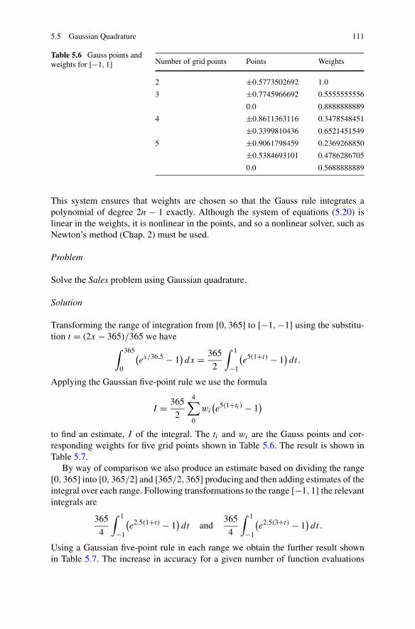
5.5 Gaussian Quadrature 111
Table 5.6 Gauss points andweights for [−1,1] Number of grid points Points Weights
2 ±0.5773502692 1.0
3 ±0.7745966692 0.5555555556
0.0 0.8888888889
4 ±0.8611363116 0.3478548451
±0.3399810436 0.6521451549
5 ±0.9061798459 0.2369268850
±0.5384693101 0.4786286705
0.0 0.5688888889
This system ensures that weights are chosen so that the Gauss rule integrates apolynomial of degree 2n − 1 exactly. Although the system of equations (5.20) islinear in the weights, it is nonlinear in the points, and so a nonlinear solver, such asNewton’s method (Chap. 2) must be used.
Problem
Solve the Sales problem using Gaussian quadrature.
Solution
Transforming the range of integration from [0,365] to [−1,−1] using the substitu-tion t = (2x − 365)/365 we have
∫ 365
0
(ex/36.5 − 1
)dx = 365
2
∫ 1
−1
(e5(1+t) − 1
)dt.
Applying the Gaussian five-point rule we use the formula
I = 365
2
4∑0
wi
(e5(1+ti ) − 1
)
to find an estimate, I of the integral. The ti and wi are the Gauss points and cor-responding weights for five grid points shown in Table 5.6. The result is shown inTable 5.7.
By way of comparison we also produce an estimate based on dividing the range[0,365] into [0,365/2] and [365/2,365] producing and then adding estimates of theintegral over each range. Following transformations to the range [−1,1] the relevantintegrals are
365
4
∫ 1
−1
(e2.5(1+t) − 1
)dt and
365
4
∫ 1
−1
(e2.5(3+t) − 1
)dt.
Using a Gaussian five-point rule in each range we obtain the further result shownin Table 5.7. The increase in accuracy for a given number of function evaluations
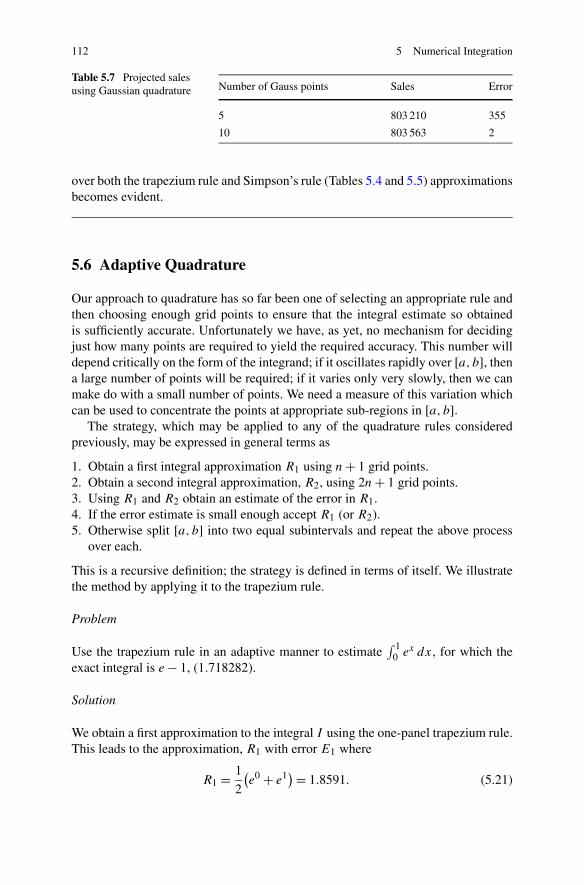
112 5 Numerical Integration
Table 5.7 Projected salesusing Gaussian quadrature Number of Gauss points Sales Error
5 803 210 355
10 803 563 2
over both the trapezium rule and Simpson’s rule (Tables 5.4 and 5.5) approximationsbecomes evident.
5.6 Adaptive Quadrature
Our approach to quadrature has so far been one of selecting an appropriate rule andthen choosing enough grid points to ensure that the integral estimate so obtainedis sufficiently accurate. Unfortunately we have, as yet, no mechanism for decidingjust how many points are required to yield the required accuracy. This number willdepend critically on the form of the integrand; if it oscillates rapidly over [a, b], thena large number of points will be required; if it varies only very slowly, then we canmake do with a small number of points. We need a measure of this variation whichcan be used to concentrate the points at appropriate sub-regions in [a, b].
The strategy, which may be applied to any of the quadrature rules consideredpreviously, may be expressed in general terms as
1. Obtain a first integral approximation R1 using n + 1 grid points.2. Obtain a second integral approximation, R2, using 2n + 1 grid points.3. Using R1 and R2 obtain an estimate of the error in R1.4. If the error estimate is small enough accept R1 (or R2).5. Otherwise split [a, b] into two equal subintervals and repeat the above process
over each.
This is a recursive definition; the strategy is defined in terms of itself. We illustratethe method by applying it to the trapezium rule.
Problem
Use the trapezium rule in an adaptive manner to estimate∫ 1
0 ex dx, for which theexact integral is e − 1, (1.718282).
Solution
We obtain a first approximation to the integral I using the one-panel trapezium rule.This leads to the approximation, R1 with error E1 where
R1 = 1
2
(e0 + e1) = 1.8591. (5.21)
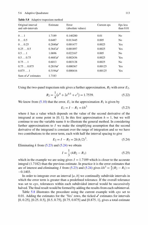
5.6 Adaptive Quadrature 113
Table 5.8 Adaptive trapezium method
Original intervaland sub-intervals
Estimate Error(absolute values)
Current eps Eps lessthan 0.01
0 . . . 1 1.7189 0.140280 0.01 No
0 . . . 0.5 0.6487 0.013445 0.005 No
0 . . . 0.25 0.2840✓ 0.001477 0.0025 Yes
0.25 . . . 0.5 0.3647✓ 0.001897 0.0025 Yes
0.5 . . . 1 1.0696 0.022167 0.005 No
0.5 . . . 0.75 0.4683✓ 0.002436 0.0025 Yes
0.75 . . . 1 0.6013 0.003128 0.0025 No
0.75 . . . 0.875 0.2819✓ 0.000367 0.00125 Yes
0.875 . . . 1 0.3194✓ 0.000416 0.00125 Yes
Sum of ✓ estimates 1.7183
Using the two-panel trapezium rule gives a further approximation, R2 with error E2.
R2 = 1
4
(e0 + 2e0.5 + e1) = 1.7539. (5.22)
We know from (5.10) that the error, E1 in the approximation R1 is given by
E1 = I − R1 = kh3 (5.23)
where k has a value which depends on the value of the second derivative of theintegrand at some point in [0,1]. In this first approximation h = 1, but we willcontinue to use the variable name h to illustrate the general method. In consideringfurther approximations to I we make the simplifying assumption that the secondderivative of the integrand is constant over the range of integration and so we havetwo contributions to the error term, each with half the interval spacing to give
E2 = I − R2 = 2k(h/2)3. (5.24)
Eliminating k from (5.23) and (5.24) we obtain
I = 1
3(4R2 − R1) (5.25)
which in the example we are using gives I = 1.7189 which is closer to the accurateintegral (1.7182) than the previous estimate. In practice it is the error estimates thatare of interest and eliminating I from (5.23) and (5.24) gives kh3 = 4
3 (R2 − R1) =−0.1403.
In order to integrate over an interval [a, b] we continually subdivide intervals inwhich the error term is greater than a predefined tolerance. If the overall tolerancewas set to eps, tolerances within each subdivided interval would be successivelyhalved. The final result would be formed by adding the results from each subinterval.
Table 5.8 illustrates the procedure using the current example with eps set to0.01. Adding the estimates for the ‘Yes’ rows, the ticked ✓ estimates for intervals[0,0.25], [0.25,0.5], [0.5,0.75], [0.75,0.875] and [0.875,1], gives a total estimate
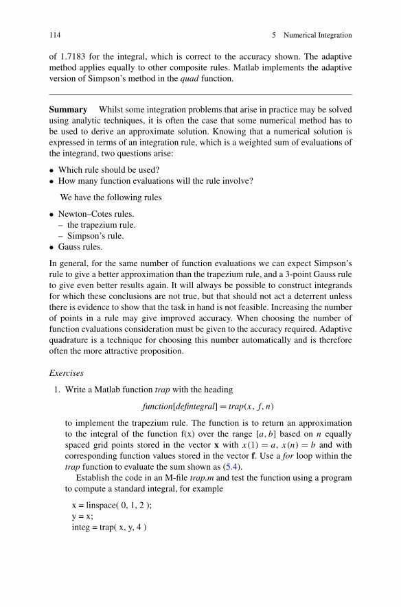
114 5 Numerical Integration
of 1.7183 for the integral, which is correct to the accuracy shown. The adaptivemethod applies equally to other composite rules. Matlab implements the adaptiveversion of Simpson’s method in the quad function.
Summary Whilst some integration problems that arise in practice may be solvedusing analytic techniques, it is often the case that some numerical method has tobe used to derive an approximate solution. Knowing that a numerical solution isexpressed in terms of an integration rule, which is a weighted sum of evaluations ofthe integrand, two questions arise:
• Which rule should be used?• How many function evaluations will the rule involve?
We have the following rules
• Newton–Cotes rules.– the trapezium rule.– Simpson’s rule.
• Gauss rules.
In general, for the same number of function evaluations we can expect Simpson’srule to give a better approximation than the trapezium rule, and a 3-point Gauss ruleto give even better results again. It will always be possible to construct integrandsfor which these conclusions are not true, but that should not act a deterrent unlessthere is evidence to show that the task in hand is not feasible. Increasing the numberof points in a rule may give improved accuracy. When choosing the number offunction evaluations consideration must be given to the accuracy required. Adaptivequadrature is a technique for choosing this number automatically and is thereforeoften the more attractive proposition.
Exercises
1. Write a Matlab function trap with the heading
function[defintegral] = trap(x, f,n)
to implement the trapezium rule. The function is to return an approximationto the integral of the function f(x) over the range [a, b] based on n equallyspaced grid points stored in the vector x with x(1) = a, x(n) = b and withcorresponding function values stored in the vector f. Use a for loop within thetrap function to evaluate the sum shown as (5.4).
Establish the code in an M-file trap.m and test the function using a programto compute a standard integral, for example
x = linspace( 0, 1, 2 );y = x;integ = trap( x, y, 4 )
5.6 Adaptive Quadrature 115
which returns in variable integ the Trapezium approximation (in this case anaccurate evaluation) to
∫ 10 x dx based on 2 grid points.
2. Evaluate∫ 1
0 x2 dx using function trap from the previous question with differentnumbers of grid points. In each case calculate the difference between the correctvalue (1/3) and the estimated value. Confirm that the difference is as predictedby (5.11). Use the formula to predict (and confirm by running the program) thata mesh of 14 points would be required for absolute error of less than 0.001.
3. Modify the Matlab code for trap to produce a function Simpson with a similarheading. Use a formula based on a more general form of (5.6) to implement themethod. Assume an odd number of grid points. Ensure that the input parametern is an odd number by using the Matlab function floor, which rounds down tothe nearest integer. Use separate loops for the odd and even sums.
function [integral] = Simpson( x, f, n )% Assume function values for the range of integration are stored in% equally spaced values x(i), y(i) i=1..n where is an odd number% if n is even print an error message and return to the calling program
if 2∗ floor( n/2 ) == n;disp('Error:number of grid points must be odd');return;
else%% Insert the Simpson code%
end;
Use the function Simpson to show that∫ 1
0 x2 dx and also∫ 1
0 x3 dx are evaluated
correctly and that the error in evaluating∫ 1
0 x4 dx are all as predicted by (5.17).4. Compare the rates at which the Simpson’s rule and the trapezium rule converge
to an estimate of ∫ 1
0
1
1 + x2dx
with increasing number of grid points. The accurate value is π/4.Note that as with element by element multiplication using the .* dot–
asterisk operator, Matlab provides a corresponding element by element divisionoperator ./ dot–slash operator and so an x, y mesh of n evenly spaced pointsspanning the interval [0,1] may be generated using the following commands:
x = linspace( 0, 1, n );y = 1 ./ sqrt(1 + x.∗x);
Use the Matlab commands trapz to apply the trapezium rule and quad based onSimpson’s rule to check the results from your own routines. For the exampleabove, assuming x and y and a function f (x) to evaluate 1/(1 + x2) werealready defined, suitable commands would be
116 5 Numerical Integration
trapz(x, y)quad(@f,0,1) % use the @ prefix to pass a function name as a parameter
In general trapz(x, y) integrates y values over corresponding x values andquad(@f,a, b) integrates the function f between the limits a and b. By defaultquad approximates to within an accuracy of 1.0e−6 and requires the functionf = f (x) = 1/(1 + x2), where x is the vector of data points, to be defined inan M-file with corresponding name f.m
5. Write a Matlab function with the heading function[points] = Gmesh(n) to gen-erate the n roots of the Legendre Polynomial Pn−1(x). Using recurrence rela-tion (5.19) we have P0 = 1, P1 = x and P2 = 1
2 (3 ∗ x2 − 1) and so since weare writing the coefficients of the first three Legendre Polynomials as Matlabvectors for use in the function roots to find the roots, we have
p = [1];q = [1 0];r = (3/2)∗ [q 0] - (1/2)∗[0 0 p];
It would be possible to continue in this way using a new variable name at eachstep. Using a matrix is a possibility but there are complications in that eachrow regarded as a vector would have one more element that the one before.A convenient option is provided by the cell structure (question 1 of Sect. 1.15.2)as shown below:
p(1) = {[1]}p(2) ={[1 0]};
Using (5.19) and noting that we are storing the coefficients of the ith polynomialin p(n) we have the Matlab expression
p(i + 2) = {((2 ∗ i + 1)/(i + 1)) ∗ [p{i + 1} 0] − (i/(i + 1)) ∗ [0 0 p{i}]};which may be incorporated in a for loop (from 1 to n − 2) within the functionGmesh. The final action of Gmesh would be to call roots with input parameter{p} to find the roots of p(n). Test the function against the values shown inTable 5.6.
6. Write a program to calculate the weights corresponding to the relative Gausspoints. Equation (5.20) shows that for the first two Legendre Polynomials, P1and P2 the linear systems to be solved are:
w1 + w2 = 2w1 + w1x2 = 0(x1 = 0.5774, x2 = −0.5774)
w1 + w2 + w3 = 2w1x1 + w2x2 + w3x3 = 0w1x1 + w2x
22 + w3x
23 = 2
3(x1 = 0, x2 = 0.7746, x3 = −0.7746).
In deriving the second system from formula (5.20), note that 00 = 1. It followsthat in the second example the leading coefficient of the first equation in thisexample will be one (and not zero). The general pattern for forming a generaln × n system may be deduced. In forming the coefficient matrix, the Matlaboperator .∧ for raising the elements of a vector (or matrix) to a given power (for

5.6 Adaptive Quadrature 117
example v = v. ∧ 2 or e = g. ∧ j ) may be useful. Test the program against thevalues shown in Table 5.6.
7. Use the Gauss 5-point rule to estimate the integral I = ∫ π2
0 sinx dx. In orderto use the rule transform the range of integration from [0,π/2] to [−1,+1] bymaking the substitution
t = −1 + 4
πx
so that when x = 0, t = −1 and when x = π2 , t = +1. We now have
I = π
4
∫ +1
−1sin
π
4(t + 1) dt.
Use the Gauss 5-point rule
I = π
4
4∑i=0
wi sinπ
4(pi + 1)
where pi and wi , i = 1, . . . ,5 are the Gauss points. The accurate value, whichmay be found analytically is 1.0.
8. Modify the function trap developed earlier to produce a new function Etrapwhich for a given function f returns an estimate of the integral
∫ b
af (x) dx using
the trapezium rule and in the notation of Sect. 5.6 the error quantity kh3. Theestimates are to be based on using just 2 and 3 grid points as described in thesolution to the problem shown in Sect. 5.8.
Use the following heading for the function
function[integral, error] = Etrap(a, b, f )
and store the program in a file Etrap.m. The program will need to call the orig-inal trap function first with parameter n set to 2 and again with n = 3.
Test the program using the example quoted in Sect. 5.6 and a command suchas Etrap(0,1,@exp) or [int, err] = Etrap(0,1,@exp); to return the values forthe estimated integral and the estimated error in variables int and err respec-tively.
9. As an introduction to the next question. Write a function fact with heading
function[Factorial] = fact(n)
to evaluate the factorial of an integer n, usually denoted by n! Use the principleof recursion by which a function is evaluated by repeatedly evaluating simplerversions of itself until a stage is reached (a stopping condition) at which a valueof the function is known. For this example a stopping condition would be 1! = 1.Following the header, a single statement of the following form will suffice
if n== 1;Factorial = 1; % stopping condition
elseFactorial = n ∗ fact(n-1);

118 5 Numerical Integration
10. Write a Matlab function Atrap which for a given function f uses AdaptiveQuadrature based on the Trapezium Rule to return an estimate of the integral∫ b
af (x) dx to within a prescribed accuracy eps. Use the following heading for
the function
function[integral] = Atrap(a, b, f, eps)
and base the program on the following recursive scheme:
% estimate the integral over the range [a, b] using Etrap (question 8)[i e] = Etrap (a, b, f); % (for example)
% is the absolute value of the estimated error returned by Etrap less than eps?% if it is
integral = i; % the stopping condition% if not, halve the interval, halve the required accuracy and try again,% by treating the two% intervals separately. Keep on doing this as long as is necessary.
eps = eps/2;integral = Atrap(a, (a+b)/2, f, eps)+ Atrap((a+b)/2, b, f, eps);
Test the program against standard integrals with known values, for example usethe command
Atrap(0,1,@exp,1.0e-006)
to validate the results shown in Table 5.8. You may like to check the progress ofthe recursion by inserting statements to display the intervals and to show howthey are subdivided to achieve the required accuracy.
Chapter 6Numerical Differentiation
Aims In this chapter we look at numerical methods for estimating derivativesof a function f = f (x). We establish formulae for evaluating f ′(x) and higherderivatives for any value of x.
Overview The methods of this chapter are not intended to be used on a func-tion for which values are only available at specific points. Although the underlyingfunction in question may be analytic, the methods assume that we can provide func-tion values wherever we are asked to do so. If the precise form of the function is notknown it is better to construct an approximation using the method of least squares orto construct a spline approximation in the manner discussed in Chap. 4 and use theresulting function to estimate derivatives. In this way a global view of the functionis taken and so is likely to produce more accurate estimates than a method whichrelies on piecemeal interpolation to supply individual values.
We point out that the methods of this chapter are also not intended to be usedwhere expressions for derivatives may be obtained without too much difficulty us-ing the rules of differential calculus. However the functions we use in illustratingthe methods will be mainly of this type as they are useful for verification purposes.Of course, any analytic function may be differentiated, but in some cases, for exam-ple in the case of complicated rationals, the actual differentiation is not for the fainthearted. In any event Matlab has facilities for displaying derivatives in symbolic(algebraic) form, which will be explained in an end-of-chapter exercise. Estimatesfor derivatives are often required in solving differential equations for which an an-alytic solution is not available. If a numerical solution is therefore the only option,progress to a solution may be made by replacing derivatives by estimates based onfunction values
The methods to be described fall into two classes. On the one hand we deriveformulae based on function values in the vicinity of the point at which we wish toestimate the derivative. In this context we derive two, three and five-point formulaebased on two, three and five local points respectively. Our second approach is totransform the problem of estimating the derivative into that of estimating the valueof an integral, a problem that has already been considered in Chap. 5.
C. Woodford, C. Phillips, Numerical Methods with Worked Examples: Matlab Edition,DOI 10.1007/978-94-007-1366-6_6, © Springer Science+Business Media B.V. 2012
119
120 6 Numerical Differentiation
Acquired Skills After reading this chapter you will be able to
• recognise the circumstances in which numerical differentiation rather than ana-lytic differentiation may be usefully applied.
• understand how two, three and five-point formulae are derived.• apply two, three and five-point formulae to finding estimates of first and higher
order derivatives.• understand how Cauchy’s theorem can be used to transform the problem of esti-
mating derivatives into that of estimating an integral from which we may obtainestimates for first and higher order derivatives.
6.1 Introduction
As is often the case in numerical analysis we take Taylor’s theorem as our startingpoint. For a function f which is continuous and has continuous derivatives in aninterval [a, b] for any points x and x + h in that interval, we have formulae such as
f (x + h) = f (x) + hf ′(x) + R1 (6.1)
f (x + h) = f (x) + hf ′(x) + h2
2! f ′′(x) + R2 (6.2)
......
f (x + h) = f (x) + hf ′(x) + h2
2! f ′′(x) + · · · + hm
m! f(m)(x) + Rm. (6.3)
In each case the remainder term Ri depends on the next higher derivative. In partic-ular
Rm = hm+1
(m + 1)!f(m+1)(ψm) (6.4)
where ψm is some point in the interval (x, x + h).
6.2 Two-Point Formula
We can use expressions (6.1)–(6.3) to provide formulae for numerical differentia-tion. For example the expression (6.1) may be written in the form
f ′(x) = f (x + h) − f (x)
h− 1
hR1 (6.5)
which leads to the approximation
f ′(x) ≈ f (x + h) − f (x)
h. (6.6)
The approximation (6.6) is known as a two-point formula, since it uses functionvalues at two points to estimate the derivative.

6.2 Two-Point Formula 121
Table 6.1 Estimates of f ′(0)
for f (x) = sin(x)n f ′(0) Error
1 0.9589 0.0411
2 0.9896 0.0104
3 0.9974 0.0026
4 0.9993 0.0007
5 0.9998 0.0002
6 1.0000 0.0000
7 1.0000 0.0000
Problem
For f (x) = sin(x) estimate f ′(x) at x = 0.
Solution
In using (6.6) we have no indication as to an appropriate value for h other than itshould be small to reduce the remainder term R1. Accordingly we start with h =0.5 and successively half the value until a consistent value for f ′ is found. Puttingx = 0 in (6.6) we obtain the results (see Table 6.1) for successive values of h, whereh = 1
2n , n = 1,2, . . ..
Discussion
The results show that (to four decimal places) the value of the derivative, f ′(0)
is 1.0000 and so the numerical approximation agrees with the analytical result(f ′(0) = cos(0) = 1). For f (x) = sinx, f ′′(x) = − sinx and so |f ′′(x)| ≤ 1. Thisimplies that the remainder term R1, which can be found from (6.4) with m = 1, is atmost h
2 whatever the value of ψ1, which in turn guarantees the accuracy of the esti-
mate for sufficiently small h. Furthermore the error, namely R1h
(the absolute valueis shown) is halved as h is halved. This is a result to be expected from (6.4). Eventhough in this case the final value h may appear to be small, even smaller valuesmay be necessary as the following example shows.
Problem
For f (x) = x5 estimate f ′(x) at x = 2.
Solution
Using (6.6) we obtain the results in Table 6.2.
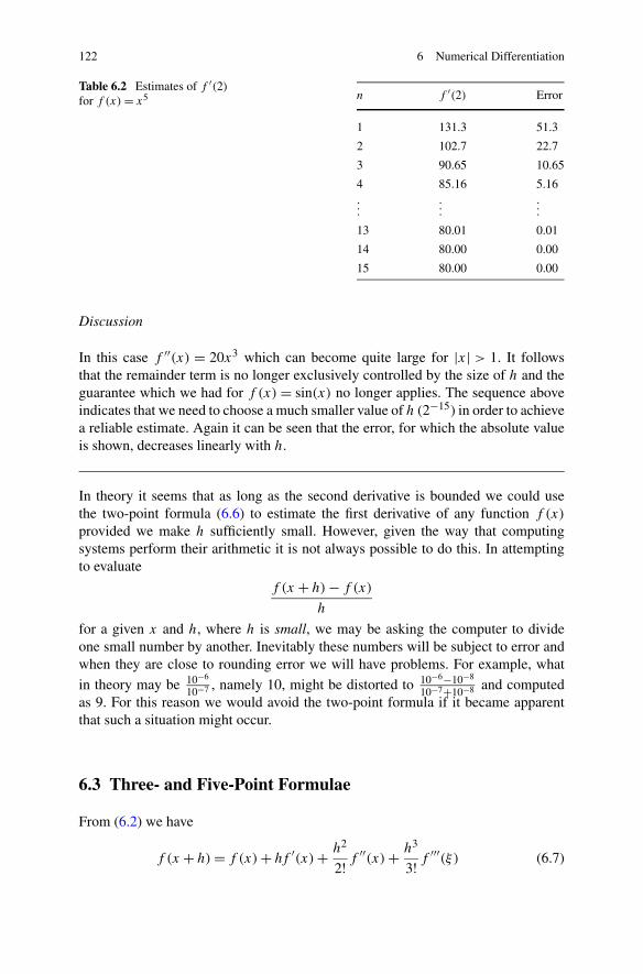
122 6 Numerical Differentiation
Table 6.2 Estimates of f ′(2)
for f (x) = x5 n f ′(2) Error
1 131.3 51.3
2 102.7 22.7
3 90.65 10.65
4 85.16 5.16...
.
.
....
13 80.01 0.01
14 80.00 0.00
15 80.00 0.00
Discussion
In this case f ′′(x) = 20x3 which can become quite large for |x| > 1. It followsthat the remainder term is no longer exclusively controlled by the size of h and theguarantee which we had for f (x) = sin(x) no longer applies. The sequence aboveindicates that we need to choose a much smaller value of h (2−15) in order to achievea reliable estimate. Again it can be seen that the error, for which the absolute valueis shown, decreases linearly with h.
In theory it seems that as long as the second derivative is bounded we could usethe two-point formula (6.6) to estimate the first derivative of any function f (x)
provided we make h sufficiently small. However, given the way that computingsystems perform their arithmetic it is not always possible to do this. In attemptingto evaluate
f (x + h) − f (x)
h
for a given x and h, where h is small, we may be asking the computer to divideone small number by another. Inevitably these numbers will be subject to error andwhen they are close to rounding error we will have problems. For example, what
in theory may be 10−6
10−7 , namely 10, might be distorted to 10−6−10−8
10−7+10−8 and computedas 9. For this reason we would avoid the two-point formula if it became apparentthat such a situation might occur.
6.3 Three- and Five-Point Formulae
From (6.2) we have
f (x + h) = f (x) + hf ′(x) + h2
2! f ′′(x) + h3
3! f ′′′(ξ) (6.7)
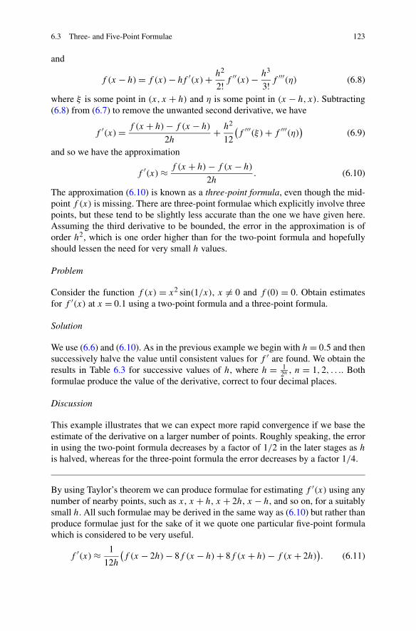
6.3 Three- and Five-Point Formulae 123
and
f (x − h) = f (x) − hf ′(x) + h2
2! f ′′(x) − h3
3! f ′′′(η) (6.8)
where ξ is some point in (x, x + h) and η is some point in (x − h,x). Subtracting(6.8) from (6.7) to remove the unwanted second derivative, we have
f ′(x) = f (x + h) − f (x − h)
2h+ h2
12
(f ′′′(ξ) + f ′′′(η)
)(6.9)
and so we have the approximation
f ′(x) ≈ f (x + h) − f (x − h)
2h. (6.10)
The approximation (6.10) is known as a three-point formula, even though the mid-point f (x) is missing. There are three-point formulae which explicitly involve threepoints, but these tend to be slightly less accurate than the one we have given here.Assuming the third derivative to be bounded, the error in the approximation is oforder h2, which is one order higher than for the two-point formula and hopefullyshould lessen the need for very small h values.
Problem
Consider the function f (x) = x2 sin(1/x), x �= 0 and f (0) = 0. Obtain estimatesfor f ′(x) at x = 0.1 using a two-point formula and a three-point formula.
Solution
We use (6.6) and (6.10). As in the previous example we begin with h = 0.5 and thensuccessively halve the value until consistent values for f ′ are found. We obtain theresults in Table 6.3 for successive values of h, where h = 1
2n , n = 1,2, . . .. Bothformulae produce the value of the derivative, correct to four decimal places.
Discussion
This example illustrates that we can expect more rapid convergence if we base theestimate of the derivative on a larger number of points. Roughly speaking, the errorin using the two-point formula decreases by a factor of 1/2 in the later stages as h
is halved, whereas for the three-point formula the error decreases by a factor 1/4.
By using Taylor’s theorem we can produce formulae for estimating f ′(x) using anynumber of nearby points, such as x, x + h, x + 2h, x − h, and so on, for a suitablysmall h. All such formulae may be derived in the same way as (6.10) but rather thanproduce formulae just for the sake of it we quote one particular five-point formulawhich is considered to be very useful.
f ′(x) ≈ 1
12h
(f (x − 2h) − 8f (x − h) + 8f (x + h) − f (x + 2h)
). (6.11)
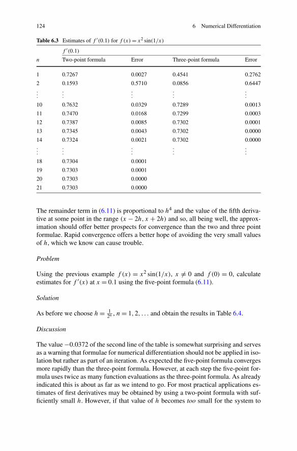
124 6 Numerical Differentiation
Table 6.3 Estimates of f ′(0.1) for f (x) = x2 sin(1/x)
f ′(0.1)
n Two-point formula Error Three-point formula Error
1 0.7267 0.0027 0.4541 0.2762
2 0.1593 0.5710 0.0856 0.6447...
.
.
....
.
.
....
10 0.7632 0.0329 0.7289 0.0013
11 0.7470 0.0168 0.7299 0.0003
12 0.7387 0.0085 0.7302 0.0001
13 0.7345 0.0043 0.7302 0.0000
14 0.7324 0.0021 0.7302 0.0000...
.
.
....
.
.
....
18 0.7304 0.0001
19 0.7303 0.0001
20 0.7303 0.0000
21 0.7303 0.0000
The remainder term in (6.11) is proportional to h4 and the value of the fifth deriva-tive at some point in the range (x − 2h,x + 2h) and so, all being well, the approx-imation should offer better prospects for convergence than the two and three pointformulae. Rapid convergence offers a better hope of avoiding the very small valuesof h, which we know can cause trouble.
Problem
Using the previous example f (x) = x2 sin(1/x), x �= 0 and f (0) = 0, calculateestimates for f ′(x) at x = 0.1 using the five-point formula (6.11).
Solution
As before we choose h = 12n , n = 1,2, . . . and obtain the results in Table 6.4.
Discussion
The value −0.0372 of the second line of the table is somewhat surprising and servesas a warning that formulae for numerical differentiation should not be applied in iso-lation but rather as part of an iteration. As expected the five-point formula convergesmore rapidly than the three-point formula. However, at each step the five-point for-mula uses twice as many function evaluations as the three-point formula. As alreadyindicated this is about as far as we intend to go. For most practical applications es-timates of first derivatives may be obtained by using a two-point formula with suf-ficiently small h. However, if that value of h becomes too small for the system to
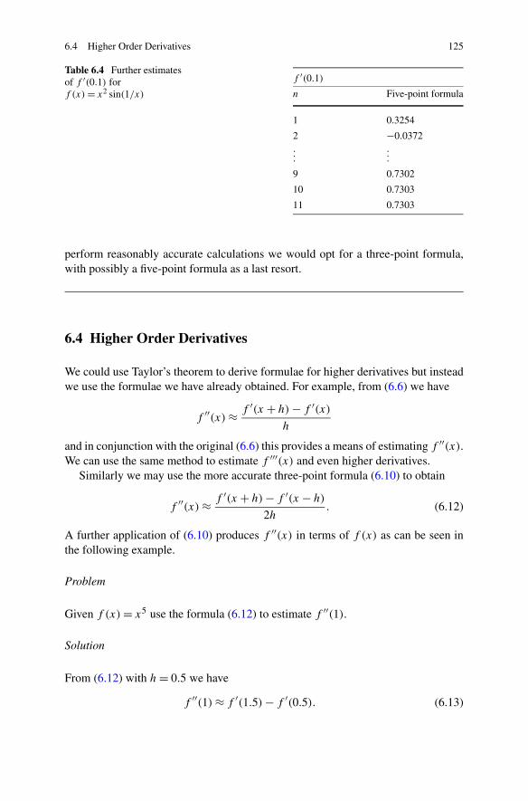
6.4 Higher Order Derivatives 125
Table 6.4 Further estimatesof f ′(0.1) forf (x) = x2 sin(1/x)
f ′(0.1)
n Five-point formula
1 0.3254
2 −0.0372...
.
.
.
9 0.7302
10 0.7303
11 0.7303
perform reasonably accurate calculations we would opt for a three-point formula,with possibly a five-point formula as a last resort.
6.4 Higher Order Derivatives
We could use Taylor’s theorem to derive formulae for higher derivatives but insteadwe use the formulae we have already obtained. For example, from (6.6) we have
f ′′(x) ≈ f ′(x + h) − f ′(x)
h
and in conjunction with the original (6.6) this provides a means of estimating f ′′(x).We can use the same method to estimate f ′′′(x) and even higher derivatives.
Similarly we may use the more accurate three-point formula (6.10) to obtain
f ′′(x) ≈ f ′(x + h) − f ′(x − h)
2h. (6.12)
A further application of (6.10) produces f ′′(x) in terms of f (x) as can be seen inthe following example.
Problem
Given f (x) = x5 use the formula (6.12) to estimate f ′′(1).
Solution
From (6.12) with h = 0.5 we have
f ′′(1) ≈ f ′(1.5) − f ′(0.5). (6.13)
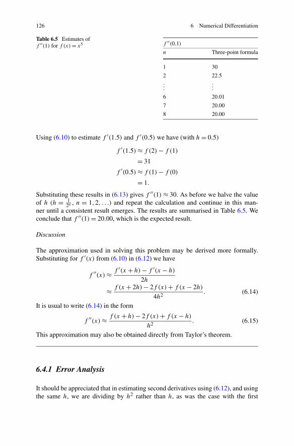
126 6 Numerical Differentiation
Table 6.5 Estimates off ′′(1) for f (x) = x5 f ′′(0.1)
n Three-point formula
1 30
2 22.5...
.
.
.
6 20.01
7 20.00
8 20.00
Using (6.10) to estimate f ′(1.5) and f ′(0.5) we have (with h = 0.5)
f ′(1.5) ≈ f (2) − f (1)
= 31
f ′(0.5) ≈ f (1) − f (0)
= 1.
Substituting these results in (6.13) gives f ′′(1) ≈ 30. As before we halve the valueof h (h = 1
2n , n = 1,2, . . .) and repeat the calculation and continue in this man-ner until a consistent result emerges. The results are summarised in Table 6.5. Weconclude that f ′′(1) = 20.00, which is the expected result.
Discussion
The approximation used in solving this problem may be derived more formally.Substituting for f ′(x) from (6.10) in (6.12) we have
f ′′(x) ≈ f ′(x + h) − f ′(x − h)
2h
≈ f (x + 2h) − 2f (x) + f (x − 2h)
4h2. (6.14)
It is usual to write (6.14) in the form
f ′′(x) ≈ f (x + h) − 2f (x) + f (x − h)
h2. (6.15)
This approximation may also be obtained directly from Taylor’s theorem.
6.4.1 Error Analysis
It should be appreciated that in estimating second derivatives using (6.12), and usingthe same h, we are dividing by h2 rather than h, as was the case with the first

6.4 Higher Order Derivatives 127
derivative. In the case of third, fourth and higher derivatives we are dividing by h3,h4 and so on. Moreover as we use a formula such as (6.12) to progress from oneorder of derivative to the next we lose an order of accuracy since the original errorterm is also divided by h. Given the previous warnings regarding h there is evenmore danger in allowing h to become too small when estimating higher derivatives.It has to be emphasised that although in theory a smaller h should lead to greateraccuracy, in practice this is not necessarily so.
Problem
Use the five-point formula (6.11) to estimate the first five derivatives of the followingfunction f (x) at x = 0
f (x) = ex
sin3 x + cos3 x.
This function is often used for test purposes since it is awkward to differentiate byhand and therefore represents the class of functions which we might well chooseto differentiate numerically. Also it can be shown that f (v)(0) = −164, which is auseful benchmark.
Solution
From (6.11) with h = 0.5 we have
f ′(0) = 1
6
(f (−1) − 8f (−0.5) + 8f (0.5) − f (1)
)
= 0.6258.
To estimate f ′′(0), using the same value of h we again use (6.11) but in the form
f ′′(0) = 1
6
(f ′(−1) − 8f ′(−0.5) + 8f ′(0.5) − f ′(1)
). (6.16)
The values of f ′ necessary to evaluate (6.16) are found by applying (6.11) in itsoriginal form. As can be seen this is quite a lengthy process, particularly by thetime we reach f (v). However, the use of recursion reduces the programming effortconsiderably.
As usual we halve the value of h (h = 12n , n = 1,2, . . .) and repeat the calcula-
tion and continue in this manner until a consistent result emerges. The results aresummarised in Table 6.6.
Discussion
We conclude that f ′(0) = 1, f ′′(0) = 4, f ′′′(0) = 4 and f (iv)(0) = 28. As forf (v)(0) we cannot be so sure. The results do not settle down in the manner of thelower derivatives and it is with less certainty that we deduce the result to be ap-proximately −164. Letting the calculation proceed with smaller and smaller valuesof h would not help. We would find that the estimates become larger and larger
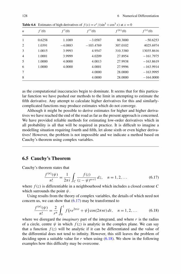
128 6 Numerical Differentiation
Table 6.6 Estimates of high derivatives of f (x) = ex/(sin3 + cos3 x) at x = 0
n f ′(0) f ′′(0) f ′′′(0) f (iv)(0) f (v)(0)
1 0.6258 1.1089 −3.0587 80.3000 −50.6253
2 1.0391 −4.0883 −103.4769 307.0102 4025.6974
3 1.0015 3.9993 4.9547 310.3380 13035.8616
4 1.0001 3.9999 4.0209 27.8954 −161.7975
5 1.0000 4.0000 4.0013 27.9938 −163.8619
6 1.0000 4.0000 4.0001 27.9996 −163.9914
7 4.0000 28.0000 −163.9995
8 4.0000 28.0000 −164.0000
as the computational inaccuracies begin to dominate. It seems that for this particu-lar function we have pushed our methods to the limit in attempting to estimate thefifth derivative. Any attempt to calculate higher derivatives for this and similarly-complicated functions may produce estimates which do not converge.
Although it might be possible to derive estimates for higher and higher deriva-tives we have reached the end of the road as far as the present approach is concerned.We have provided reliable methods for estimating low-order derivatives which inall probability is all that will be required in practice. It is difficult to imagine amodelling situation requiring fourth and fifth, let alone sixth or even higher deriva-tives! However, the problem is not impossible and we indicate a method based onCauchy’s theorem using complex variables.
6.5 Cauchy’s Theorem
Cauchy’s theorem states that
f (n)(ψ)
n! = 1
2πi
∫
C
f (z)
(z − ψ)n+1dz, n = 1,2, . . . (6.17)
where f (z) is differentiable in a neighbourhood which includes a closed contour C
which surrounds the point ψ .Using results from the theory of complex variables, the details of which need not
concern us, we can show that (6.17) may be transformed to
f (n)(ψ)
n! = 2
rn
∫ 1
0f
(re2πit + ψ
)cos(2πnt) dt, n = 1,2, . . . (6.18)
where we disregard the imaginary part of the integrand, and where r is the radiusof a circle, centre ψ in which f (z) is analytic in the complex plane. We can saythat a function f (z) will be analytic if it can be differentiated and the value ofthe differential does not tend to infinity. However, this still leaves the problem ofdeciding upon a suitable value for r when using (6.18). We show in the followingexamples how this difficulty may be overcome.
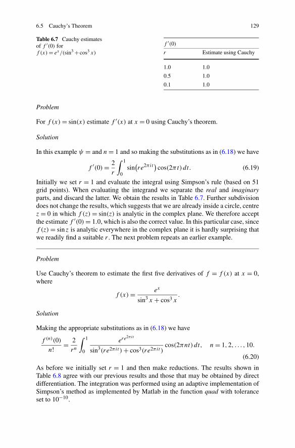
6.5 Cauchy’s Theorem 129
Table 6.7 Cauchy estimatesof f ′(0) forf (x) = ex/(sin3 + cos3 x)
f ′(0)
r Estimate using Cauchy
1.0 1.0
0.5 1.0
0.1 1.0
Problem
For f (x) = sin(x) estimate f ′(x) at x = 0 using Cauchy’s theorem.
Solution
In this example ψ = and n = 1 and so making the substitutions as in (6.18) we have
f ′(0) = 2
r
∫ 1
0sin
(re2πit
)cos(2πt) dt. (6.19)
Initially we set r = 1 and evaluate the integral using Simpson’s rule (based on 51grid points). When evaluating the integrand we separate the real and imaginaryparts, and discard the latter. We obtain the results in Table 6.7. Further subdivisiondoes not change the results, which suggests that we are already inside a circle, centrez = 0 in which f (z) = sin(z) is analytic in the complex plane. We therefore acceptthe estimate f ′(0) = 1.0, which is also the correct value. In this particular case, sincef (z) = sin z is analytic everywhere in the complex plane it is hardly surprising thatwe readily find a suitable r . The next problem repeats an earlier example.
Problem
Use Cauchy’s theorem to estimate the first five derivatives of f = f (x) at x = 0,where
f (x) = ex
sin3 x + cos3 x.
Solution
Making the appropriate substitutions as in (6.18) we have
f (n)(0)
n! = 2
rn
∫ 1
0
ere2πit
sin3(re2πit ) + cos3(re2πit )cos(2πnt) dt, n = 1,2, . . . ,10.
(6.20)
As before we initially set r = 1 and then make reductions. The results shown inTable 6.8 agree with our previous results and those that may be obtained by directdifferentiation. The integration was performed using an adaptive implementation ofSimpson’s method as implemented by Matlab in the function quad with toleranceset to 10−10.
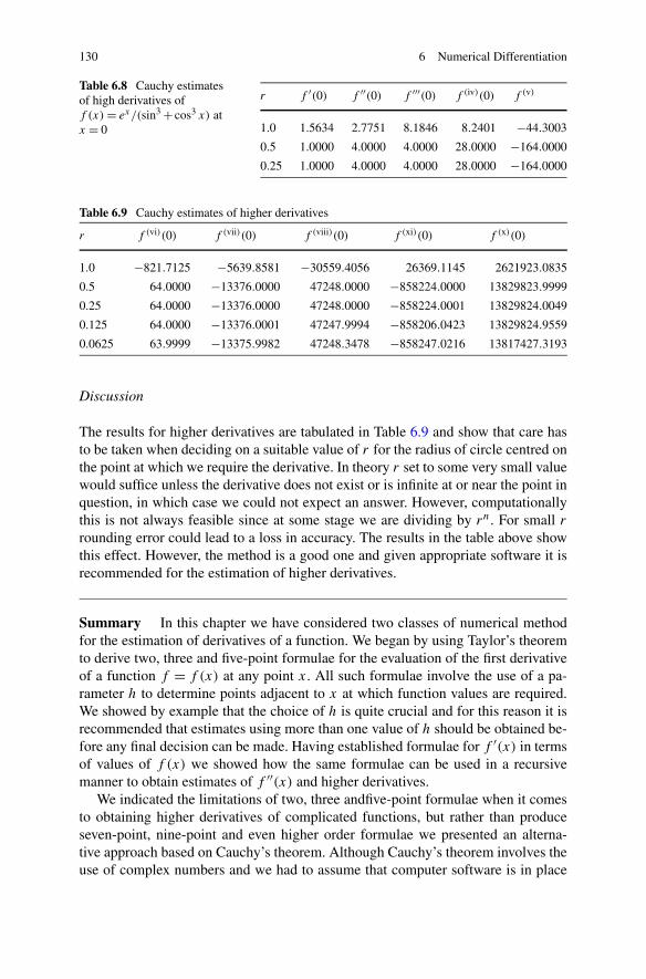
130 6 Numerical Differentiation
Table 6.8 Cauchy estimatesof high derivatives off (x) = ex/(sin3 + cos3 x) atx = 0
r f ′(0) f ′′(0) f ′′′(0) f (iv)(0) f (v)
1.0 1.5634 2.7751 8.1846 8.2401 −44.3003
0.5 1.0000 4.0000 4.0000 28.0000 −164.0000
0.25 1.0000 4.0000 4.0000 28.0000 −164.0000
Table 6.9 Cauchy estimates of higher derivatives
r f (vi)(0) f (vii)(0) f (viii)(0) f (xi)(0) f (x)(0)
1.0 −821.7125 −5639.8581 −30559.4056 26369.1145 2621923.0835
0.5 64.0000 −13376.0000 47248.0000 −858224.0000 13829823.9999
0.25 64.0000 −13376.0000 47248.0000 −858224.0001 13829824.0049
0.125 64.0000 −13376.0001 47247.9994 −858206.0423 13829824.9559
0.0625 63.9999 −13375.9982 47248.3478 −858247.0216 13817427.3193
Discussion
The results for higher derivatives are tabulated in Table 6.9 and show that care hasto be taken when deciding on a suitable value of r for the radius of circle centred onthe point at which we require the derivative. In theory r set to some very small valuewould suffice unless the derivative does not exist or is infinite at or near the point inquestion, in which case we could not expect an answer. However, computationallythis is not always feasible since at some stage we are dividing by rn. For small r
rounding error could lead to a loss in accuracy. The results in the table above showthis effect. However, the method is a good one and given appropriate software it isrecommended for the estimation of higher derivatives.
Summary In this chapter we have considered two classes of numerical methodfor the estimation of derivatives of a function. We began by using Taylor’s theoremto derive two, three and five-point formulae for the evaluation of the first derivativeof a function f = f (x) at any point x. All such formulae involve the use of a pa-rameter h to determine points adjacent to x at which function values are required.We showed by example that the choice of h is quite crucial and for this reason it isrecommended that estimates using more than one value of h should be obtained be-fore any final decision can be made. Having established formulae for f ′(x) in termsof values of f (x) we showed how the same formulae can be used in a recursivemanner to obtain estimates of f ′′(x) and higher derivatives.
We indicated the limitations of two, three andfive-point formulae when it comesto obtaining higher derivatives of complicated functions, but rather than produceseven-point, nine-point and even higher order formulae we presented an alterna-tive approach based on Cauchy’s theorem. Although Cauchy’s theorem involves theuse of complex numbers and we had to assume that computer software is in place
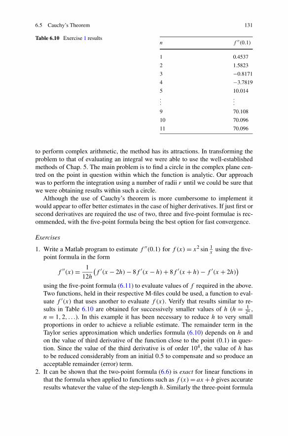
6.5 Cauchy’s Theorem 131
Table 6.10 Exercise 1 resultsn f ′′(0.1)
1 0.4537
2 1.5823
3 −0.8171
4 −3.7819
5 10.014...
.
.
.
9 70.108
10 70.096
11 70.096
to perform complex arithmetic, the method has its attractions. In transforming theproblem to that of evaluating an integral we were able to use the well-establishedmethods of Chap. 5. The main problem is to find a circle in the complex plane cen-tred on the point in question within which the function is analytic. Our approachwas to perform the integration using a number of radii r until we could be sure thatwe were obtaining results within such a circle.
Although the use of Cauchy’s theorem is more cumbersome to implement itwould appear to offer better estimates in the case of higher derivatives. If just first orsecond derivatives are required the use of two, three and five-point formulae is rec-ommended, with the five-point formula being the best option for fast convergence.
Exercises
1. Write a Matlab program to estimate f ′′(0.1) for f (x) = x2 sin 1x
using the five-point formula in the form
f ′′(x) = 1
12h
(f ′(x − 2h) − 8f ′(x − h) + 8f ′(x + h) − f ′(x + 2h)
)
using the five-point formula (6.11) to evaluate values of f required in the above.Two functions, held in their respective M-files could be used, a function to eval-uate f ′(x) that uses another to evaluate f (x). Verify that results similar to re-sults in Table 6.10 are obtained for successively smaller values of h (h = 1
2n ,n = 1,2, . . .). In this example it has been necessary to reduce h to very smallproportions in order to achieve a reliable estimate. The remainder term in theTaylor series approximation which underlies formula (6.10) depends on h andon the value of third derivative of the function close to the point (0.1) in ques-tion. Since the value of the third derivative is of order 104, the value of h hasto be reduced considerably from an initial 0.5 to compensate and so produce anacceptable remainder (error) term.
2. It can be shown that the two-point formula (6.6) is exact for linear functions inthat the formula when applied to functions such as f (x) = ax + b gives accurateresults whatever the value of the step-length h. Similarly the three-point formula

132 6 Numerical Differentiation
(6.10) is exact for quadratic polynomials and the five-point formula (6.11) is ex-act for quartic polynomials. Write a program to check these statements by eval-uating f ′(x) for (i) a linear function using the two-step formula, (ii) a quadraticpolynomial using the three-step formula and (iii) a quartic polynomial using thefive-point formulae. In each case use arbitrary values for x, step-length h and forfunction coefficients.
3. It is possible to produce formulae for estimating derivatives based on values toone side of the point in question. Using techniques similar to those we havealready discussed it can be shown that
f ′(x) ≈ −3f (x) + 4f (x + h) − f (x + 2h)
2h
and
f ′(x) ≈ −25f (x) + 48f (x + h) − 36f (x + 2h) + 16f (x + 3h) − 3f (x + 4h)
12h
are alternative three- and five-point formulae. Show by experiment that in generalthese formulae are not quite as effective as their more balanced counterparts(6.10) and (6.11) and so should only be used when values of the function f arenot available at one side or the other of the point in question.
4. This exercise aims to estimate the derivatives of
f (x) = ex
sin3 x + cos3 x
at x = 0 and so confirm the results quoted in the chapter.(i) Write a Matlab function chy with heading
function [chyval] = chy(t)
to evaluate the integrand of (6.20) for any given value of t and constant values r
and n. Note that Matlab has facilities for handling complex (imaginary) numbersincluding arithmetic involving combinations of real and complex numbers. Ingeneral the complex number a + ib (a, b real) may be written as complex (a, b)or a + bi (it is important to place i next to b and to separate the sign). The usualarithmetic operations apply.
The variables r and n, are to be declared as global since they are to be givenvalues from the program which will use chy and so the function might have theform
function[chyval] = chy(t)global n r;c= r ∗ exp(2∗pi∗complex(0, 1) ∗ t);% using the .∗ and .∧ element by element multiplication and% exponentiation operatorschyval = exp(c).∗cos(2∗pi∗n∗t) ./ (sin(c).∧ 3 + cos(c).∧3);
Having stored the function in an M-file chy, test the function using the program
6.5 Cauchy’s Theorem 133
global n rr = 1; n =1;chy(0.5);
to confirm that(
eeπi
sin3(eπi) + cos3(eπi)
)cos(π) = 0.8397.
(ii) Evaluate the integral
f (n)(0)
n! = 2
rn
∫ 1
0
(ere2πit
sin3(eπi) + cos3(eπi)
)cos(2πnt) dt, n = 1,2, . . . ,10
using the Matlab function quad with tolerance 1.0e-11. Express the real part ofthe integrand using the function real as in the following code
c= r∗ exp(2∗pi∗complex(0, 1)∗t);% Recover the real part of a complex numberrp = real (exp(c).∗cos(2∗pi∗n∗t) ./ (sin(c) .∧ 3 + cos(c) .∧3))
5. The Matlab Symbolic Math Toolbox provides tools for solving and manipulatingsymbolic (i.e. algebraic) expressions, including the function diff for differentiat-ing. Use the following program to evaluate symbolically the first, second, third,fourth and fifth derivatives of the function f at the point x = 0.
syms f d x; % declare f d and x to be symbolic variablesf = exp(x)/(sin(x)∧3 + cos(x)∧3);x = 0;d = diff(f); % differentiate f symbolicallyeval(d) % evaluate the first differential at x = 0for i = 1 : 4
d = diff(d) % evaluate next differential from the one beforeeval(d) % evaluate at x = 0
end;
The symbolic expressions for the derivatives may be seen by removing the trail-ing semi-colons but not surprisingly they are quite lengthy. The function ezplotis available for plotting symbolic expressions. Enter the command help ezplot forfurther details.
Chapter 7Linear Programming
Aims In this chapter we
• explain what is meant by a linear programming problem.• show how linear programming problems arise in the real-world.• show how a simple linear programming problem may be solved by graphical
methods
and then, taking the lead from this graphical approach, devise
• the simplex method for solving linear programming problems.
Finally we consider
• the ‘travelling salesman problem’ as it is traditionally known: deciding the short-est route through a number of cities
and
• the ‘machine scheduling problem’: completing in the shortest possible time aseries of processes competing for shared resources.
Overview Linear programming is concerned with finding the maximum value ofa real-valued linear function f of a number of variables. We may also be asked tofind the minimum value of f , but this is equivalent to finding the maximum value of−f and so there is no additional problem. Such a linear function might, for example,be given by f = f (x1, x2), where f = x1 + 2x2, although in practice many morevariables are usually involved. The function in question is known as the objectivefunction. Additionally, the dependent variables (x1, x2 in the case quoted above),are required to satisfy a number of linear relations, known as constraints. Thus alinear programming problem might be to find values of x1, x2 that
maximise z = x1 + 2x2subject to 3x1 + 2x2 ≤ 5
x1 + 3x2 ≤ 6x1, x2 ≥ 0.
C. Woodford, C. Phillips, Numerical Methods with Worked Examples: Matlab Edition,DOI 10.1007/978-94-007-1366-6_7, © Springer Science+Business Media B.V. 2012
135
136 7 Linear Programming
The solution to a linear programming problem is known as the optimal solution.We may further impose the condition that some or all of the variables may only takeinteger values at the optimal solution. This leads to a branch of linear programmingknown as integer programming, or mixed integer programming (if not all vari-ables are so constrained). A byproduct of integer programming enables us to modelthe decision making process when faced with alternative strategies in the search foran optimum solution.
It is worth remarking that the term linear programming has no connection withcomputer programming as such. Linear programming began life in earnest duringWorld War II when it was used by the military in making decisions regarding theoptimum deployment of equipment and supplies.
Acquired Skills After reading this chapter and completing the exercises you willbe able to
• recognise if a problem is suitable for linear programming.• model the problem in a standard form.• solve a two variable problem using graphical methods.• use the simplex method to solve a more general problem.• use the branch and bound method to solve an integer programming problem (and
a mixed integer programming problem).• set up linear programming models incorporating decision making.
7.1 Introduction
Problems from the real world rarely present themselves in a form which is immedi-ately amenable to linear programming. It is often the case that simplifications haveto be made in order that the objective function and the constraints may be repre-sented as linear functions. Even if a problem is recognised as being suitable forlinear programming, data must be collected and tabulated. The skill in successfullinear programming lies in the modelling of the problem and in the interpretationof the consequent solution. The calculations involved in finding the solution to alinear programming problem follow a well-defined path, which may be best left toa computer.
7.2 Forming a Linear Programming Problem
By way of an example we consider a problem that we refer to as the garment factoryproblem. Although only two variables are involved, it is indicative of the way inwhich larger problems are modelled.
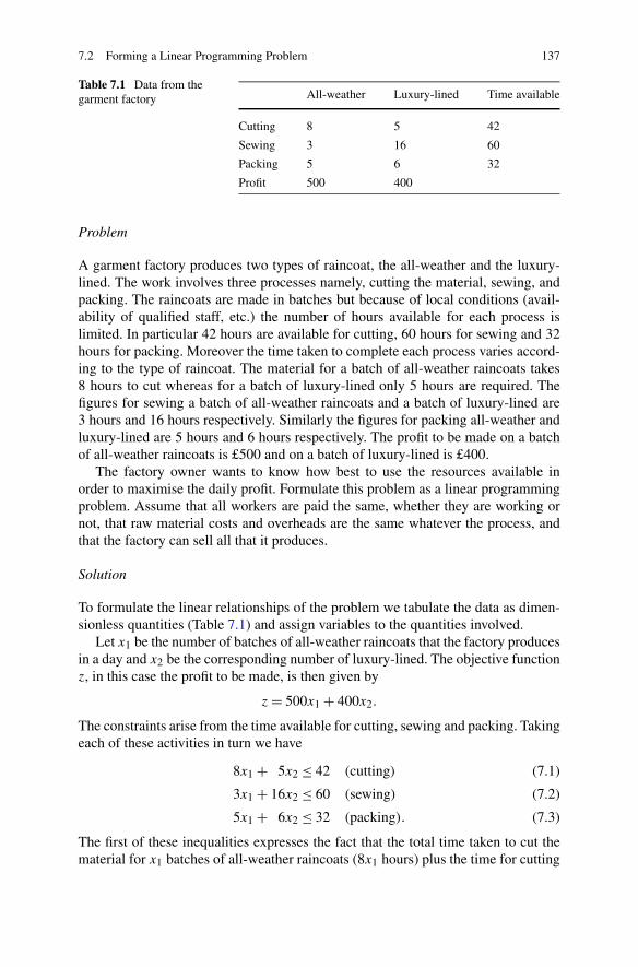
7.2 Forming a Linear Programming Problem 137
Table 7.1 Data from thegarment factory All-weather Luxury-lined Time available
Cutting 8 5 42
Sewing 3 16 60
Packing 5 6 32
Profit 500 400
Problem
A garment factory produces two types of raincoat, the all-weather and the luxury-lined. The work involves three processes namely, cutting the material, sewing, andpacking. The raincoats are made in batches but because of local conditions (avail-ability of qualified staff, etc.) the number of hours available for each process islimited. In particular 42 hours are available for cutting, 60 hours for sewing and 32hours for packing. Moreover the time taken to complete each process varies accord-ing to the type of raincoat. The material for a batch of all-weather raincoats takes8 hours to cut whereas for a batch of luxury-lined only 5 hours are required. Thefigures for sewing a batch of all-weather raincoats and a batch of luxury-lined are3 hours and 16 hours respectively. Similarly the figures for packing all-weather andluxury-lined are 5 hours and 6 hours respectively. The profit to be made on a batchof all-weather raincoats is £500 and on a batch of luxury-lined is £400.
The factory owner wants to know how best to use the resources available inorder to maximise the daily profit. Formulate this problem as a linear programmingproblem. Assume that all workers are paid the same, whether they are working ornot, that raw material costs and overheads are the same whatever the process, andthat the factory can sell all that it produces.
Solution
To formulate the linear relationships of the problem we tabulate the data as dimen-sionless quantities (Table 7.1) and assign variables to the quantities involved.
Let x1 be the number of batches of all-weather raincoats that the factory producesin a day and x2 be the corresponding number of luxury-lined. The objective functionz, in this case the profit to be made, is then given by
z = 500x1 + 400x2.
The constraints arise from the time available for cutting, sewing and packing. Takingeach of these activities in turn we have
8x1 + 5x2 ≤ 42 (cutting) (7.1)
3x1 + 16x2 ≤ 60 (sewing) (7.2)
5x1 + 6x2 ≤ 32 (packing). (7.3)
The first of these inequalities expresses the fact that the total time taken to cut thematerial for x1 batches of all-weather raincoats (8x1 hours) plus the time for cutting
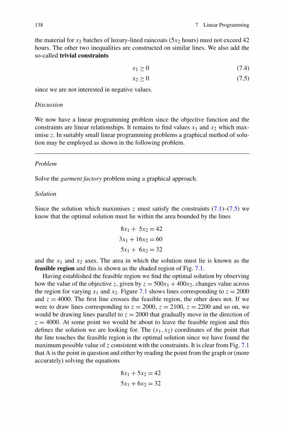
138 7 Linear Programming
the material for x2 batches of luxury-lined raincoats (5x2 hours) must not exceed 42hours. The other two inequalities are constructed on similar lines. We also add theso-called trivial constraints
x1 ≥ 0 (7.4)
x2 ≥ 0 (7.5)
since we are not interested in negative values.
Discussion
We now have a linear programming problem since the objective function and theconstraints are linear relationships. It remains to find values x1 and x2 which max-imise z. In suitably small linear programming problems a graphical method of solu-tion may be employed as shown in the following problem.
Problem
Solve the garment factory problem using a graphical approach.
Solution
Since the solution which maximises z must satisfy the constraints (7.1)–(7.5) weknow that the optimal solution must lie within the area bounded by the lines
8x1 + 5x2 = 42
3x1 + 16x2 = 60
5x1 + 6x2 = 32
and the x1 and x2 axes. The area in which the solution must lie is known as thefeasible region and this is shown as the shaded region of Fig. 7.1.
Having established the feasible region we find the optimal solution by observinghow the value of the objective z, given by z = 500x1 + 400x2, changes value acrossthe region for varying x1 and x2. Figure 7.1 shows lines corresponding to z = 2000and z = 4000. The first line crosses the feasible region, the other does not. If wewere to draw lines corresponding to z = 2000, z = 2100, z = 2200 and so on, wewould be drawing lines parallel to z = 2000 that gradually move in the direction ofz = 4000. At some point we would be about to leave the feasible region and thisdefines the solution we are looking for. The (x1, x2) coordinates of the point thatthe line touches the feasible region is the optimal solution since we have found themaximum possible value of z consistent with the constraints. It is clear from Fig. 7.1that A is the point in question and either by reading the point from the graph or (moreaccurately) solving the equations
8x1 + 5x2 = 42
5x1 + 6x2 = 32
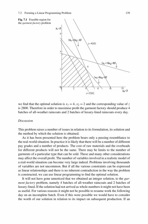
7.2 Forming a Linear Programming Problem 139
Fig. 7.1 Feasible region forthe garment factory problem
we find that the optimal solution is x1 = 4, x2 = 2 and the corresponding value of z
is 2800. Therefore in order to maximise profit the garment factory should produce 4batches of all-weather raincoats and 2 batches of luxury-lined raincoats every day.
Discussion
This problem raises a number of issues in relation to its formulation, its solution andthe method by which the solution is obtained.
As it has been presented here the problem bears only a passing resemblance tothe real-world situation. In practice it is likely that there will be a number of differentpay grades and a number of products. The cost of raw materials and the overheadsfor different products will not be the same. There may be limits to the number ofgarments of a particular type that can be sold. These and many other considerationsmay affect the overall profit. The number of variables involved in a realistic model ofa real-world situation can become very large indeed. Problems involving thousandsof variables are not uncommon. But if all the various constraints can be expressedas linear relationships and there is no inherent contradiction in the way the problemis constructed, we can use linear programming to find the optimal solution.
It will not have gone unnoticed that we obtained an integer solution, to the gar-ment factory problem, namely 4 batches of all-weather raincoats and 2 batches ofluxury-lined. If the solution had not arrived as whole numbers it might not have beenas useful. For various reasons it might not be possible to resume work the followingday on an incomplete batch. Even if this were possible we would have to considerthe worth of our solution in relation to its impact on subsequent production. If an
140 7 Linear Programming
integer solution is the only one that is acceptable we can force the issue by usinginteger programming, which is to be discussed later in the chapter.
Given the way in which we found the solution to our problem, by moving a straightline across the feasible region, it is to be expected that the solution is found at acorner (or vertex) of the feasible region. This principle extends to more complexproblems. If we have a problem involving three variables we would have a feasibleregion in the form of a three-dimensional shape made up of flat (two-dimensional)surfaces. If this is the case we can imagine the objective function as a plane movingthrough the polyhedral figure and reaching its maximum value at a vertex. We havetheorems which state that if the feasible region of a linear programming problemis bounded then the feasible region has a polyhedral shape and that if a linear pro-gramming problem has an optimal solution then the optimal solution is found at avertex of the feasible region.
It might appear to be a simple matter to evaluate the objective at every feasiblevertex and note where the highest value of the objective occurs. However, whilstsuch an approach would work for small problems, it becomes totally impracticalfor larger problems. Even to identify the feasible region of a linear programmingproblem having just 16 problem variables and subject to 20 non-trivial constraintswould involve examining the 7,000 million or so points at which both trivial andnon-trivial constraints intersect. In any event such a problem is very small by linearprogramming standards. Clearly a more subtle approach is required.
However, the graphical approach has served to indicate the way ahead using amethod based on the vertices of the feasible region. In the following we adopt analgebraic approach, but in order to do this we require linear programming problemsto be expressed in a common form.
7.3 Standard Form
For a linear programming problem involving n variables x1, x2, . . . , xn we maywrite the objective z as
z = c1x1 + c2x2 + · · · + cnxn.
In the language of linear programming the variables x1, x2, . . . , xn are known asproblem variables and the coefficients c1, c2, . . . , cn are known as costs. Since theproblem of maximising z is the same as that of minimising −z we assume as a firststep towards standard form that the problem is always one of finding a set of valuesof the problem variables which maximises the objective. If necessary we replaceeach ci by −ci and ignore any fixed price (constant overhead) costs.
As a further step towards standardisation we express all constraints (other thanthe trivial constraints) using the ≤ sign. Again, this may be achieved by changingsigns of the appropriate coefficients.
7.4 Canonical Form 141
It follows that any linear programming problem may be expressed in the form
maximise z = c1x1 + c2x2 + · · · + cnxn
subject to c11x1 + c12x2 + · · · + c1nxn ≤ b1c21x1 + c22x2 + · · · + c2nxn ≤ b2...
...
cm1x1 + cm2x2 + · · · + cmnxn ≤ bm
x1, x2, . . . , xn ≥ 0
which is known as the standard form.
Problem
Write the following linear programming problem in standard form
minimise −x1 + 3x2 − 4x3subject to 2x1 + 4x3 ≤ 4
x1 + x2 − 5x3 ≥ 42x2 − x3 ≥ 2
x1, x2, x3 ≥ 0.
Solution
By a judicious change of signs we can rearrange the problem to
maximise x1 − 3x2 + 4x3subject to 2x1 + 4x3 ≤ 4
−x1 − x2 + 5x3 ≤ 4−2x2 + x3 ≤ 2
x1, x2, x3 ≥ 0.
7.4 Canonical Form
From standard form we move to what proves to be the more useful canonical form.We write the non-trivial constraints as equalities. This is achieved by the introduc-tion of extra variables, known as slack variables, which are constrained to be ≥ 0.For example, a constraint such as
2x1 + 4x3 ≤ 4
may be re-written as
2x1 + 4x3 + x4 = 4
x4 ≥ 0
by the introduction of the slack variable x4. The subscript 4 is chosen as being thenext available following the sequence of subscripts already allocated.
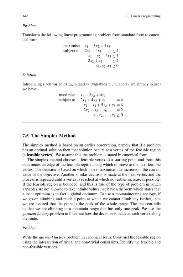
142 7 Linear Programming
Problem
Transform the following linear programming problem from standard form to canon-ical form
maximise x1 − 3x2 + 4x3subject to 2x1 + 4x3 ≤ 4
−x1 − x2 + 5x3 ≤ 4−2x2 + x3 ≤ 2
x1, x2, x3 ≥ 0.
Solution
Introducing slack variables x4, x5 and x6 (variables x1, x2 and x3 are already in use)we have
maximise x1 − 3x2 + 4x3subject to 2x1 + 4x3 + x4 = 4
−x1 − x2 + 5x3 + x5 = 4−2x2 + x3 + x6 = 2
x1, x2, . . . , x6 ≥ 0.
7.5 The Simplex Method
The simplex method is based on an earlier observation, namely that if a problemhas an optimal solution then that solution occurs at a vertex of the feasible region(a feasible vertex). We assume that the problem is stated in canonical form.
The simplex method chooses a feasible vertex as a starting point and from thisdetermines an edge of the feasible region along which to move to the next feasiblevertex. The decision is based on which move maximises the increase in the currentvalue of the objective. Another similar decision is made at the next vertex and theprocess is repeated until a vertex is reached at which no further increase is possible.If the feasible region is bounded, and this is true of the type of problem in whichvariables are not allowed to take infinite values, we have a theorem which states thata local optimum is in fact a global optimum. To use a mountaineering analogy, ifwe go on climbing and reach a point at which we cannot climb any further, thenwe are assured that the point is the peak of the whole range. The theorem tellsus that we are climbing in a mountain range that has only one peak. We use thegarment factory problem to illustrate how the decision is made at each vertex alongthe route.
Problem
Write the garment factory problem in canonical form. Construct the feasible regionusing the intersection of trivial and non-trivial constraints. Identify the feasible andnon-feasible vertices.
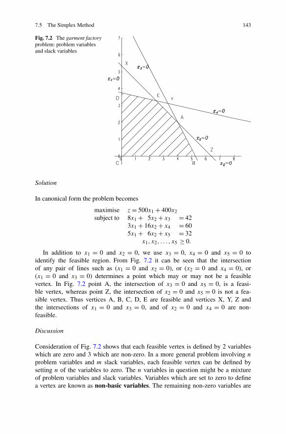
7.5 The Simplex Method 143
Fig. 7.2 The garment factoryproblem: problem variablesand slack variables
Solution
In canonical form the problem becomes
maximise z = 500x1 + 400x2subject to 8x1 + 5x2 + x3 = 42
3x1 + 16x2 + x4 = 605x1 + 6x2 + x5 = 32
x1, x2, . . . , x5 ≥ 0.
In addition to x1 = 0 and x2 = 0, we use x3 = 0, x4 = 0 and x5 = 0 toidentify the feasible region. From Fig. 7.2 it can be seen that the intersectionof any pair of lines such as (x1 = 0 and x2 = 0), or (x2 = 0 and x4 = 0), or(x1 = 0 and x3 = 0) determines a point which may or may not be a feasiblevertex. In Fig. 7.2 point A, the intersection of x3 = 0 and x5 = 0, is a feasi-ble vertex, whereas point Z, the intersection of x2 = 0 and x5 = 0 is not a fea-sible vertex. Thus vertices A, B, C, D, E are feasible and vertices X, Y, Z andthe intersections of x1 = 0 and x3 = 0, and of x2 = 0 and x4 = 0 are non-feasible.
Discussion
Consideration of Fig. 7.2 shows that each feasible vertex is defined by 2 variableswhich are zero and 3 which are non-zero. In a more general problem involving n
problem variables and m slack variables, each feasible vertex can be defined bysetting n of the variables to zero. The n variables in question might be a mixtureof problem variables and slack variables. Variables which are set to zero to definea vertex are known as non-basic variables. The remaining non-zero variables are

144 7 Linear Programming
Table 7.2 Feasible verticesof the garment factoryproblem
Vertex Basic variables Non-basic variables
A x1, x2, x4 x3, x5
B x1, x4, x5 x2, x3
C x3, x4, x5 x1, x2
D x2, x3, x5 x1, x4
E x1, x2, x3 x4, x5
known as basic variables. Furthermore, the set of values of the variables (bothproblem variables and slack variables) at a feasible vertex is known as a basic fea-sible solution. Table 7.2 shows which variables are basic and which are non-basic,at the feasible vertices A, B, . . . , E. It can be seen that moving along an edge ofthe feasible region from one vertex to the next is equivalent to making a non-basicvariable become basic and making a basic variable become non-basic. A feature ofthe simplex method is the shuffling of variables between the basic and non-basicsets.
It is usual to start with the all slack solution, that is the point defined by setting allproblem variables to zero. If this point is a feasible vertex then we may proceed. Ifnot we have to look elsewhere for a feasible vertex with which to start the method.
We are now in a position to state the simplex method using terms we have intro-duced.
• Find a basic feasible solution.• Consider the possible routes along the edges of the feasible region to nearby ver-
tices. Choose the route which produces the greatest increase in the objective func-tion. If no such route exists we have an optimal solution and the method termi-nates.
• Move along the chosen route to the next vertex and repeat the previous step.
The following problem indicates how these steps are carried out.
Problem
Use the simplex method to find a solution to the garment factory problem.
Solution
For convenience we repeat the canonical form of the problem namely, maximisez = 500x1 + 400x2 subject to
8x1 + 5x2 + x3 = 42 (7.6)
3x1 + 16x2 + x4 = 60 (7.7)
5x1 + 6x2 + x5 = 32 (7.8)
x1, x2, . . . , x5 ≥ 0. (7.9)
7.5 The Simplex Method 145
We start with the all-slack solution, that is x1 = 0 and x2 = 0, a point which fromFig. 7.2 can be seen to be a feasible solution. In the absence of such a diagram weset x1 and x2 to zero in (7.6)–(7.8) and find that x3, x4 and x5 take the values 42,60 and 32 respectively. These values are positive and so none of the constraints ofis violated. We therefore have a basic feasible solution.
It is clear that increasing x1 (from zero) is going to make for a greater increasein the objective z than a corresponding increase in x2. In short, we look for the non-basic variable with the largest positive coefficient in the objective function. Accord-ingly we let x1 become non-zero, that is we make x1 a basic variable and determinewhich current basic variable should become non-basic.
Equations (7.6)–(7.8) may be re-written as
x3 = 42 − 8x1 − 5x2
x4 = 60 − 3x1 − 16x2
x5 = 32 − 5x1 − 6x2.
By comparing the ratios 42/8, 60/3 and 32/5 (the constant term divided by thecoefficient of x1) and noting that 42/8 is the smallest of these, it can be seen that asx1 increases from zero (and x2 remains zero), the first of x3, x4 and x5 (the non-basicvariables) to become zero is x3. Therefore having let x1 become basic, x3 becomesnon-basic. We have therefore moved along the edge from C to B in Fig. 7.2.
We repeat the procedure at B. We have to decide which of the non-basic variablesbecoming non-zero will have the greater effect on the objective z. We have
z = 500x1 + 400x2
which in terms of the non-basic variables (now x2 and x3) becomes
z = 500(42 − 5x2 − x3)/8 + 400x2
= 2625 + 87.5x2 − 62.5x3. (7.10)
It follows that x2 should become a basic variable, as x2 becoming non-zero hasgreater effect on increasing z than x3 becoming non-zero. In fact, because the co-efficient of x3 is negative we can exclude it from consideration. To decide whichof the basic variables at B should become non-basic we re-write (7.6)–(7.8), withthe basic variables gathered on the left-hand side. Since x3 is to remain non-basic(zero), we have
x1 = (42 − 5x2)/8 (7.11)
3x1 + x4 = 60 − 16x2 (7.12)
5x1 + x5 = 32 − 6x2. (7.13)
Using (7.11) in (7.12) and (7.13) we have
x4 = (354 − 113x2)/8x5 = (46 − 23x2)/8.
(7.14)
146 7 Linear Programming
Of the ratios 42/5, 354/113 and 46/23, the smallest is 46/23 and so x5 is the firstvariable to become zero as x2 increases from zero. We choose the smallest value sothat all the variables remain non-negative. We therefore make x5 non-basic, whichin addition to having made x2 basic moves us from point B to point A.
We repeat the procedure at A. Once again we look at the objective in terms of thenon-basic variables (now x3 and x5). Using (7.10) and (7.14) we have
z = 2625 − 87.5(8x5 − 46)/23 − 62.5x3
= 2800 − 62.5x3 − (700/23)x5.
We are now in the interesting position of being unable to increase the value of theobjective since either x3 or x5 increasing from zero has a negative effect. We con-clude that we are at the optimal solution, namely z = 2800. Putting x3 = 0 andx5 = 0 in the constraint equations gives
8x1 + 5x2 = 42
5x1 + 6x2 = 32.
Solving, we find that x1 = 4 and x2 = 2. This is the same solution that we obtainedby graphical means.
Discussion
In this particular example we worked our way through the simplex method in arather ad hoc, manner dealing with problems as they arose. Further problems mayarise if one or more of the variables in a basic solution is zero. We may cycle rounda sequence of vertices without increasing the value of the objective function.
Since linear programming problems often involve thousands of variables consider-able effort has been invested into making computer programs for linear program-ming as efficient as possible. The most popular version is known as the revisedsimplex method which, with very little extra effort, simultaneously solves a lin-ear programming problem (known as the dual) similar to the original in additionto the original (known as the primal) and in so doing provides some indication ateach stage as to how far we are from the optimal solution and how susceptible theoptimal solution is to changes in the data.
7.5.1 Starting the Simplex Method
As already indicated, if the all-slack solution is feasible then this is an obviouschoice with which to start the simplex method. If the all-slack solution is not feasiblewe must look elsewhere. Though possible for smaller problems, randomly selectingvariables to be non-basic (zero) could be too time consuming if applied to larger
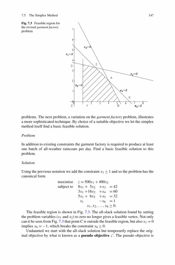
7.5 The Simplex Method 147
Fig. 7.3 Feasible region forthe revised garment factoryproblem
problems. The next problem, a variation on the garment factory problem, illustratesa more sophisticated technique. By choice of a suitable objective we let the simplexmethod itself find a basic feasible solution.
Problem
In addition to existing constraints the garment factory is required to produce at leastone batch of all-weather raincoats per day. Find a basic feasible solution to thisproblem.
Solution
Using the previous notation we add the constraint x1 ≥ 1 and so the problem has thecanonical form
maximise z = 500x1 + 400x2subject to 8x1 + 5x2 +x3 = 42
3x1 +16x2 +x4 = 605x1 + 6x2 +x5 = 32x1 −x6 = 1
x1, x2, . . . , x6 ≥ 0.
The feasible region is shown in Fig. 7.3. The all-slack solution found by settingthe problem variables (x1 and x2) to zero no longer gives a feasible vertex. Not onlycan it be seen from Fig. 7.3 that point C is outside the feasible region, but also x1 = 0implies x6 = −1, which breaks the constraint x6 ≥ 0.
Undaunted we start with the all-slack solution but temporarily replace the orig-inal objective by what is known as a pseudo objective z′. The pseudo objective is
148 7 Linear Programming
chosen with the aim of increasing the value of x6 and hopefully making it positive.We use the simplex method with the objective z′ given by z′ = x6 and the originalconstraints.
We have z′ = x6 = x1 − 1 and so choosing x1 rather than x2 to become non-zero from the list of non-basic variables (x1, x2) has the greater effect on z′. So x1becomes a basic variable. The basic variables are currently x3, x4, x5 and x6, sokeeping x2 zero we have
x3 = 42 − 8x1
x4 = 60 − 3x1
x5 = 32 − 5x1
x6 = −1 + x1.
As x1 increases from zero it is clear that x6 will be the first variable to becomezero, and so x6 becomes non-basic. We now have x2 = 0 and x6 = 0, from which itfollows that x1 = 1, x3 = 34, x4 = 57 and x5 = 27. This is a basic feasible solutionto the original problem and so it can be used to start the simplex method proper.
Discussion
In effect one step of the simplex method using the pseudo objective has taken usfrom point C to point Y in Fig. 7.3. If this had not been a feasible vertex we wouldhave tried another step but with a different pseudo objective; in such a case thepseudo objective would be the sum of all the negative variables. If the original linearprogramming problem involves equality constraints the following problem showshow to overcome this particular difficulty.
Problem
In addition to the original constraints the garment factory is required to produceexactly 6 batches of coats per day. The requirement that at least one batch of all-weather raincoats be produced no longer applies. Find a basic feasible solution.
Solution
The problem has the canonical form
maximise z = 500x1 + 400x2subject to 8x1 + 5x2 +x3 = 42
3x1 +16x2 +x4 = 605x1 + 6x2 +x5 = 32x1 + x2 +x6 = 6
x1, x2, . . . , x5 ≥ 0, x6 = 0.
In addition to the usual slack variables we introduce a so-called artificial variablex6. The variable is artificial in the sense that, unlike the problem variables and the
7.6 Integer Programming 149
slack variables, it is required to be zero. As with the previous problem an all-slacksolution is not possible since setting the problem variables (x1 and x2) to zero im-plies x6 = 6 which breaks the constraint x6 = 0.
Since we wish to reduce the value of x6 (to zero) we use one step of the simplexmethod with the objective z′ given by z′ = −x6 and the original constraints. Thuswe are seeking to maximise −x6, which is to minimise x6.
We have
z′ = −x6
= x1 + x2 − 6
and so we choose x1 to become a basic variable. In this case we could have equallywell chosen x2. The basic variables are currently x3, x4, x5 and x6, so keeping x2
zero we have
x3 = 42 − 8x1
x4 = 60 − 3x1
x5 = 32 − 5x1
x6 = 6 − x1.
As x1 increases from zero it is clear that x3 will be the first variable to becomezero, and so x3 becomes non-basic. We now have x2 = 0 and x3 = 0, from which itfollows that x1 = 6, x4 = 42, x5 = 2 and x6 = 0. None of the constraints are violatedand so we have a basic feasible solution with which to start the simplex method.
Discussion
In general, if the all-slack solution cannot be used to start the simplex method be-cause it is not a basic feasible solution, we look for a basic feasible solution usingthe pseudo objective
∑
xi<0
xi −∑
xi>0xi artificial
xi.
7.6 Integer Programming
We reconsider the original garment factory problem but simplified to the extent thatjust two processes are involved, namely cutting and sewing. However we add theconstraint that only complete batches of raincoats can be manufactured in any oneday. Once again we look for the most profitable manufacturing strategy.
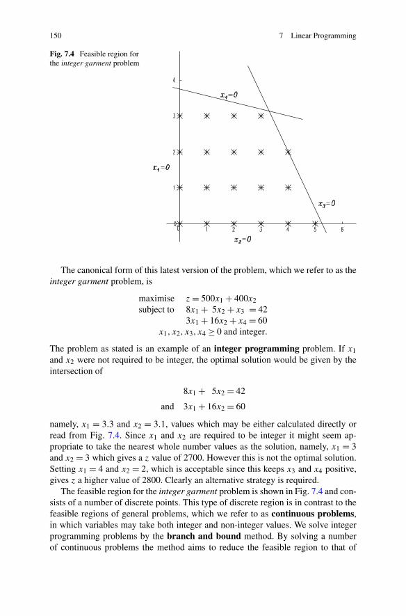
150 7 Linear Programming
Fig. 7.4 Feasible region forthe integer garment problem
The canonical form of this latest version of the problem, which we refer to as theinteger garment problem, is
maximise z = 500x1 + 400x2subject to 8x1 + 5x2 + x3 = 42
3x1 + 16x2 + x4 = 60x1, x2, x3, x4 ≥ 0 and integer.
The problem as stated is an example of an integer programming problem. If x1
and x2 were not required to be integer, the optimal solution would be given by theintersection of
8x1 + 5x2 = 42
and 3x1 + 16x2 = 60
namely, x1 = 3.3 and x2 = 3.1, values which may be either calculated directly orread from Fig. 7.4. Since x1 and x2 are required to be integer it might seem ap-propriate to take the nearest whole number values as the solution, namely, x1 = 3and x2 = 3 which gives a z value of 2700. However this is not the optimal solution.Setting x1 = 4 and x2 = 2, which is acceptable since this keeps x3 and x4 positive,gives z a higher value of 2800. Clearly an alternative strategy is required.
The feasible region for the integer garment problem is shown in Fig. 7.4 and con-sists of a number of discrete points. This type of discrete region is in contrast to thefeasible regions of general problems, which we refer to as continuous problems,in which variables may take both integer and non-integer values. We solve integerprogramming problems by the branch and bound method. By solving a numberof continuous problems the method aims to reduce the feasible region to that of
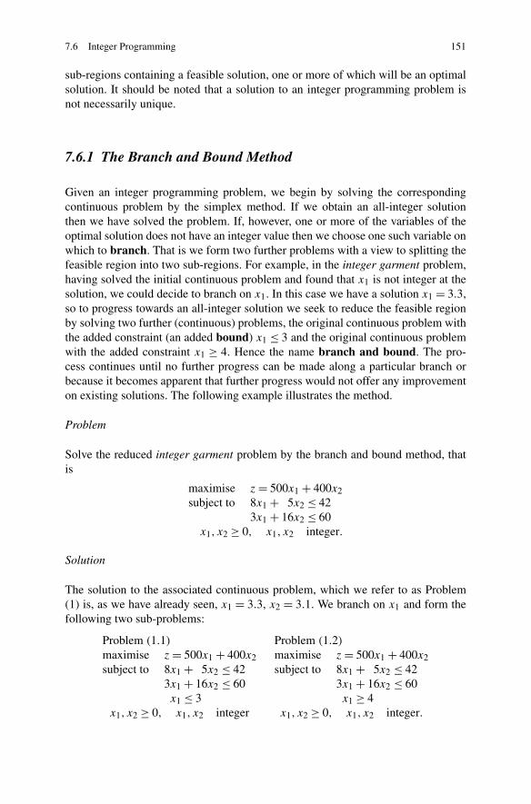
7.6 Integer Programming 151
sub-regions containing a feasible solution, one or more of which will be an optimalsolution. It should be noted that a solution to an integer programming problem isnot necessarily unique.
7.6.1 The Branch and Bound Method
Given an integer programming problem, we begin by solving the correspondingcontinuous problem by the simplex method. If we obtain an all-integer solutionthen we have solved the problem. If, however, one or more of the variables of theoptimal solution does not have an integer value then we choose one such variable onwhich to branch. That is we form two further problems with a view to splitting thefeasible region into two sub-regions. For example, in the integer garment problem,having solved the initial continuous problem and found that x1 is not integer at thesolution, we could decide to branch on x1. In this case we have a solution x1 = 3.3,so to progress towards an all-integer solution we seek to reduce the feasible regionby solving two further (continuous) problems, the original continuous problem withthe added constraint (an added bound) x1 ≤ 3 and the original continuous problemwith the added constraint x1 ≥ 4. Hence the name branch and bound. The pro-cess continues until no further progress can be made along a particular branch orbecause it becomes apparent that further progress would not offer any improvementon existing solutions. The following example illustrates the method.
Problem
Solve the reduced integer garment problem by the branch and bound method, thatis
maximise z = 500x1 + 400x2subject to 8x1 + 5x2 ≤ 42
3x1 + 16x2 ≤ 60x1, x2 ≥ 0, x1, x2 integer.
Solution
The solution to the associated continuous problem, which we refer to as Problem(1) is, as we have already seen, x1 = 3.3, x2 = 3.1. We branch on x1 and form thefollowing two sub-problems:
Problem (1.1)
maximise z = 500x1 + 400x2subject to 8x1 + 5x2 ≤ 42
3x1 + 16x2 ≤ 60x1 ≤ 3
x1, x2 ≥ 0, x1, x2 integer
Problem (1.2)
maximise z = 500x1 + 400x2subject to 8x1 + 5x2 ≤ 42
3x1 + 16x2 ≤ 60x1 ≥ 4
x1, x2 ≥ 0, x1, x2 integer.
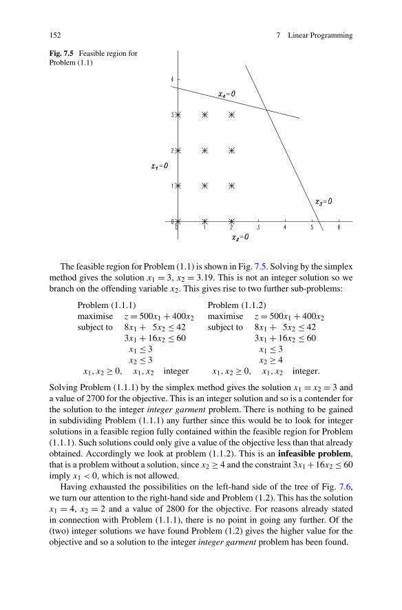
152 7 Linear Programming
Fig. 7.5 Feasible region forProblem (1.1)
The feasible region for Problem (1.1) is shown in Fig. 7.5. Solving by the simplexmethod gives the solution x1 = 3, x2 = 3.19. This is not an integer solution so webranch on the offending variable x2. This gives rise to two further sub-problems:
Problem (1.1.1)
maximise z = 500x1 + 400x2subject to 8x1 + 5x2 ≤ 42
3x1 + 16x2 ≤ 60x1 ≤ 3x2 ≤ 3
x1, x2 ≥ 0, x1, x2 integer
Problem (1.1.2)
maximise z = 500x1 + 400x2subject to 8x1 + 5x2 ≤ 42
3x1 + 16x2 ≤ 60x1 ≤ 3x2 ≥ 4
x1, x2 ≥ 0, x1, x2 integer.
Solving Problem (1.1.1) by the simplex method gives the solution x1 = x2 = 3 anda value of 2700 for the objective. This is an integer solution and so is a contender forthe solution to the integer integer garment problem. There is nothing to be gainedin subdividing Problem (1.1.1) any further since this would be to look for integersolutions in a feasible region fully contained within the feasible region for Problem(1.1.1). Such solutions could only give a value of the objective less than that alreadyobtained. Accordingly we look at problem (1.1.2). This is an infeasible problem,that is a problem without a solution, since x2 ≥ 4 and the constraint 3x1 +16x2 ≤ 60imply x1 < 0, which is not allowed.
Having exhausted the possibilities on the left-hand side of the tree of Fig. 7.6,we turn our attention to the right-hand side and Problem (1.2). This has the solutionx1 = 4, x2 = 2 and a value of 2800 for the objective. For reasons already statedin connection with Problem (1.1.1), there is no point in going any further. Of the(two) integer solutions we have found Problem (1.2) gives the higher value for theobjective and so a solution to the integer integer garment problem has been found.
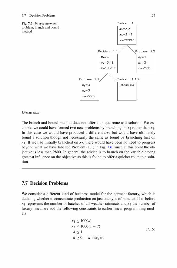
7.7 Decision Problems 153
Fig. 7.6 Integer garmentproblem, branch and boundmethod
Discussion
The branch and bound method does not offer a unique route to a solution. For ex-ample, we could have formed two new problems by branching on x2 rather than x1.In this case we would have produced a different tree but would have ultimatelyfound a solution though not necessarily the same as found by branching first onx1. If we had initially branched on x2, there would have been no need to progressbeyond what we have labelled Problem (1.1) in Fig. 7.6, since at this point the ob-jective is less than 2800. In general the advice is to branch on the variable havinggreatest influence on the objective as this is found to offer a quicker route to a solu-tion.
7.7 Decision Problems
We consider a different kind of business model for the garment factory, which isdeciding whether to concentrate production on just one type of raincoat. If as beforex1 represents the number of batches of all-weather raincoats and x2 the number ofluxury-lined, we add the following constraints to earlier linear programming mod-els
x1 ≤ 1000d
x2 ≤ 1000(1 − d)
d ≤ 1
d ≥ 0, d integer.
(7.15)

154 7 Linear Programming
Table 7.3 Car hire company, model data
Auto. gears Sun roof Child seat Hatch-back CD Route finder Immobiliser
Model 1 Yes No Yes No Yes No No
Model 2 Yes No No Yes No Yes No
Model 3 No Yes Yes No No Yes No
Model 4 No No No Yes No Yes Yes
Model 5 Yes Yes No No No No Yes
Model 6 Yes No No No Yes Yes No
Here d is a decision variable. A decision variable is a problem variable con-strained to take either the value 0 or 1. The number 1000 is somewhat arbi-trary; any number as large or larger than the greater of the possible x1 andx2 values will do. If d takes the value 1 in the optimal solution this indicatesthat all-weather raincoats are to be made, if d takes the value 0 this indicatesluxury-lined are to be made. Examples of the use of decision variables fol-low.
Problem
A car hire company offers a number of models to its customers. As can be seen fromTable 7.3, not all models have the same features. The car hire company wishes toreduce the number of models available to the minimum while retaining sufficientmodels to offer at least one car having at least one of the current seven featureson offer. Formulate the problem the company faces as a linear programming prob-lem.
Solution
We use decision variables d1, d2, . . . , d6. di = 1 indicates that model i is to be re-tained; di = 0 indicates that model i is not to be retained. The objective z which weseek to minimise is the number of models, therefore
z = d1 + d2 + d3 + d4 + d5 + d6.
The requirement that at least one model is available with automatic gears may beexpressed as
d1 + d2 + d5 + d6 ≥ 1
since only models 1,2,5 and 6 have this feature. Similar expressions apply to theother features, so we have
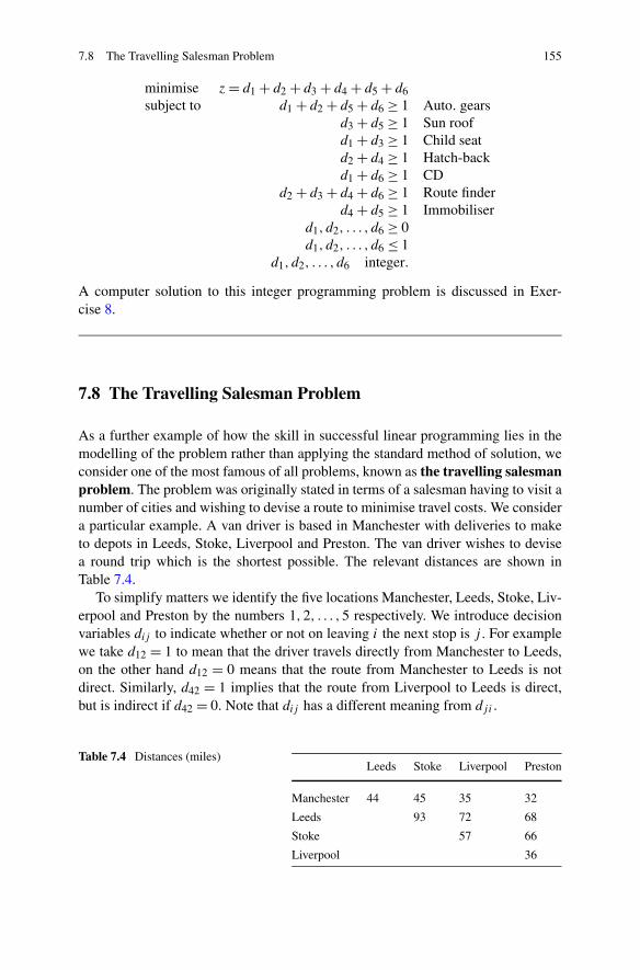
7.8 The Travelling Salesman Problem 155
minimise z = d1 + d2 + d3 + d4 + d5 + d6subject to d1 + d2 + d5 + d6 ≥ 1 Auto. gears
d3 + d5 ≥ 1 Sun roofd1 + d3 ≥ 1 Child seatd2 + d4 ≥ 1 Hatch-backd1 + d6 ≥ 1 CD
d2 + d3 + d4 + d6 ≥ 1 Route finderd4 + d5 ≥ 1 Immobiliser
d1, d2, . . . , d6 ≥ 0d1, d2, . . . , d6 ≤ 1
d1, d2, . . . , d6 integer.
A computer solution to this integer programming problem is discussed in Exer-cise 8.
7.8 The Travelling Salesman Problem
As a further example of how the skill in successful linear programming lies in themodelling of the problem rather than applying the standard method of solution, weconsider one of the most famous of all problems, known as the travelling salesmanproblem. The problem was originally stated in terms of a salesman having to visit anumber of cities and wishing to devise a route to minimise travel costs. We considera particular example. A van driver is based in Manchester with deliveries to maketo depots in Leeds, Stoke, Liverpool and Preston. The van driver wishes to devisea round trip which is the shortest possible. The relevant distances are shown inTable 7.4.
To simplify matters we identify the five locations Manchester, Leeds, Stoke, Liv-erpool and Preston by the numbers 1,2, . . . ,5 respectively. We introduce decisionvariables dij to indicate whether or not on leaving i the next stop is j . For examplewe take d12 = 1 to mean that the driver travels directly from Manchester to Leeds,on the other hand d12 = 0 means that the route from Manchester to Leeds is notdirect. Similarly, d42 = 1 implies that the route from Liverpool to Leeds is direct,but is indirect if d42 = 0. Note that dij has a different meaning from dji .
Table 7.4 Distances (miles)Leeds Stoke Liverpool Preston
Manchester 44 45 35 32
Leeds 93 72 68
Stoke 57 66
Liverpool 36
156 7 Linear Programming
The objective z which we are seeking to minimise is given by
z =5∑
i,j=1i �=j
mij dij
where mij is the distance between depots i and j , as shown in the table above.Now for the constraints. The solution is to take just one route out of Manchester
and this may be expressed as
d12 + d13 + d14 + d15 = 1.
Similarly, having made the first call, wherever that happens to be, we require justone route out. This applies to each of the other locations and so we also have
d21 + d23 + d24 + d25 = 1
d31 + d32 + d34 + d35 = 1
d41 + d42 + d43 + d45 = 1
d51 + d52 + d53 + d54 = 1.
So far so good, but this is not a complete model. We do not allow solutions whichinclude visiting the same depot twice on the grounds that a circular route is bound tobe more direct. In order to exclude combinations such as Manchester to Liverpool(d14 = 1) and Preston to Liverpool (d54 = 1) we need to specify that in addition tojust one route leading out, each location has just one route leading in. We have
d21 + d31 + d41 + d51 = 1
d12 + d32 + d42 + d52 = 1
d13 + d23 + d43 + d53 = 1
d14 + d24 + d34 + d54 = 1
d15 + d25 + d35 + d45 = 1.
In addition we have
dij ≥ 0, dij ≤ 1, dij integer.
A computer solution is discussed in Exercise 9.
7.9 The Machine Scheduling Problem
As a final example of forming a linear programming model we consider a machinescheduling problem. In general this is concerned with allocating machines, or pro-cesses, as part of a larger process in such a way that the total work in hand maybe completed as quickly as possible. To illustrate the technique we consider thefollowing problem.
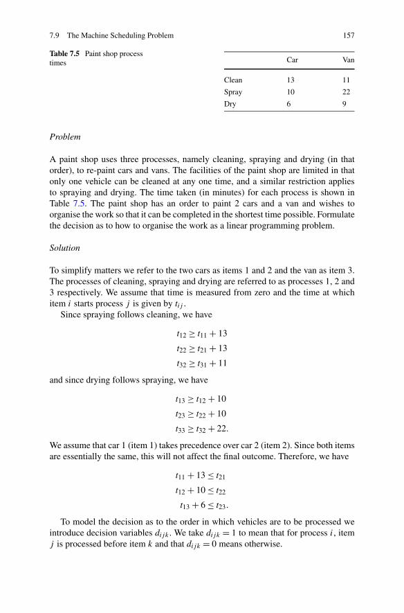
7.9 The Machine Scheduling Problem 157
Table 7.5 Paint shop processtimes Car Van
Clean 13 11
Spray 10 22
Dry 6 9
Problem
A paint shop uses three processes, namely cleaning, spraying and drying (in thatorder), to re-paint cars and vans. The facilities of the paint shop are limited in thatonly one vehicle can be cleaned at any one time, and a similar restriction appliesto spraying and drying. The time taken (in minutes) for each process is shown inTable 7.5. The paint shop has an order to paint 2 cars and a van and wishes toorganise the work so that it can be completed in the shortest time possible. Formulatethe decision as to how to organise the work as a linear programming problem.
Solution
To simplify matters we refer to the two cars as items 1 and 2 and the van as item 3.The processes of cleaning, spraying and drying are referred to as processes 1, 2 and3 respectively. We assume that time is measured from zero and the time at whichitem i starts process j is given by tij .
Since spraying follows cleaning, we have
t12 ≥ t11 + 13
t22 ≥ t21 + 13
t32 ≥ t31 + 11
and since drying follows spraying, we have
t13 ≥ t12 + 10
t23 ≥ t22 + 10
t33 ≥ t32 + 22.
We assume that car 1 (item 1) takes precedence over car 2 (item 2). Since both itemsare essentially the same, this will not affect the final outcome. Therefore, we have
t11 + 13 ≤ t21
t12 + 10 ≤ t22
t13 + 6 ≤ t23.
To model the decision as to the order in which vehicles are to be processed weintroduce decision variables dijk . We take dijk = 1 to mean that for process i, itemj is processed before item k and that dijk = 0 means otherwise.
158 7 Linear Programming
If, for example, item 1 is to go through process 1 before item 3, that is if the firstcar is to be cleaned before the van, we have
t11 + 13 ≤ t31 and d113 = 1, d131 = 0.
If this were not the case, we would have
t31 + 11 ≤ t11 and d131 = 1, d113 = 0.
These two constraints may be written as
t11 + 13 ≤ t31 + 1000(1 − d113)
t31 + 11 ≤ t11 + 1000d113.
This device neatly expresses the either–or condition in a manner similar to thatshown in (7.15). If, for example, d113 = 1, the second of the constraints is automati-cally satisfied no matter what the values of t31 and t11 (within reason) and so has noimpact. The constraint has been placed well outside the feasible region. Similarly,if d113 = 0 the first constraint becomes redundant and the second takes effect. Notethat there is now no need for a separate variable d131.
We can write similar expressions by regarding items 2 and 3 for process 1:
t21 + 13 ≤ t31 + 1000(1 − d123)
t31 + 11 ≤ t21 + 1000d123.
Similar expressions apply to the other processes. For process 2
t12 + 10 ≤ t32 + 1000(1 − d213)
t32 + 22 ≤ t12 + 1000d213
t22 + 10 ≤ t32 + 1000(1 − d223)
t32 + 22 ≤ t22 + 1000d223
and for process 3
t13 + 6 ≤ t33 + 1000(1 − d313)
t33 + 9 ≤ t13 + 1000d313
t23 + 6 ≤ t33 + 1000(1 − d323)
t33 + 9 ≤ t23 + 1000d323.
To complete the specification of the constraints we have for relevant i and j
tij ≥ 0
di13, di23 ≥ 0, di13, di23 ≤ 1
di13, di23 integer.
We now consider the objective z. We are looking to complete all three processesfor all three items in as short a time as possible, so we are looking to minimisewhatever happens to be the greater value of t23 + 6 and t33 + 9, the times at which
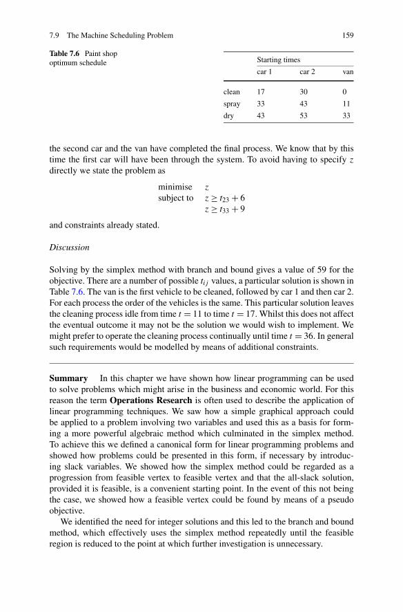
7.9 The Machine Scheduling Problem 159
Table 7.6 Paint shopoptimum schedule Starting times
car 1 car 2 van
clean 17 30 0
spray 33 43 11
dry 43 53 33
the second car and the van have completed the final process. We know that by thistime the first car will have been through the system. To avoid having to specify z
directly we state the problem as
minimise z
subject to z ≥ t23 + 6z ≥ t33 + 9
and constraints already stated.
Discussion
Solving by the simplex method with branch and bound gives a value of 59 for theobjective. There are a number of possible tij values, a particular solution is shown inTable 7.6. The van is the first vehicle to be cleaned, followed by car 1 and then car 2.For each process the order of the vehicles is the same. This particular solution leavesthe cleaning process idle from time t = 11 to time t = 17. Whilst this does not affectthe eventual outcome it may not be the solution we would wish to implement. Wemight prefer to operate the cleaning process continually until time t = 36. In generalsuch requirements would be modelled by means of additional constraints.
Summary In this chapter we have shown how linear programming can be usedto solve problems which might arise in the business and economic world. For thisreason the term Operations Research is often used to describe the application oflinear programming techniques. We saw how a simple graphical approach couldbe applied to a problem involving two variables and used this as a basis for form-ing a more powerful algebraic method which culminated in the simplex method.To achieve this we defined a canonical form for linear programming problems andshowed how problems could be presented in this form, if necessary by introduc-ing slack variables. We showed how the simplex method could be regarded as aprogression from feasible vertex to feasible vertex and that the all-slack solution,provided it is feasible, is a convenient starting point. In the event of this not beingthe case, we showed how a feasible vertex could be found by means of a pseudoobjective.
We identified the need for integer solutions and this led to the branch and boundmethod, which effectively uses the simplex method repeatedly until the feasibleregion is reduced to the point at which further investigation is unnecessary.

160 7 Linear Programming
Fig. 7.7 Feasible region for Exercise 1
Finally we showed how linear programming can model the decision-making pro-cess through the use of decision variables. This is an area which offers scope forconsiderable ingenuity in the modelling process and as such may present moreproblems than simply applying the solution process. In this context we examinedthe travelling salesman problem and the machine scheduling problem.
Exercises
1. Sketch or use Matlab to produce a diagram to confirm Fig. 7.7 is the feasibleregion for the following linear programming problem.
maximise z = 5x + 2y
subject to x + y ≤ 154x + 9y ≤ 80
4x − y ≥ 0and x, y ≥ 0.
A Matlab program based on the following scheme would be appropriate
% draw the line y = 4x using 100 equally spaced x values in the rangex = linspace( 0, 20, 100 );pc set the axis limitsaxis ([ 0 20 0 10 ]);y = 4∗x;
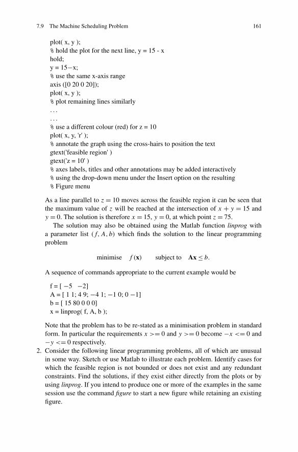
7.9 The Machine Scheduling Problem 161
plot( x, y );% hold the plot for the next line, y = 15 - xhold;y = 15−x;% use the same x-axis rangeaxis ([0 20 0 20]);plot( x, y );% plot remaining lines similarly. . .
. . .
% use a different colour (red) for z = 10plot( x, y, 'r' );% annotate the graph using the cross-hairs to position the textgtext('feasible region' )gtext('z = 10' )% axes labels, titles and other annotations may be added interactively% using the drop-down menu under the Insert option on the resulting% Figure menu
As a line parallel to z = 10 moves across the feasible region it can be seen thatthe maximum value of z will be reached at the intersection of x + y = 15 andy = 0. The solution is therefore x = 15, y = 0, at which point z = 75.
The solution may also be obtained using the Matlab function linprog witha parameter list (f,A,b) which finds the solution to the linear programmingproblem
minimise f (x) subject to Ax ≤ b.
A sequence of commands appropriate to the current example would be
f = [ −5 −2]A = [ 1 1; 4 9; −4 1; −1 0; 0 −1]b = [ 15 80 0 0 0]x = linprog( f, A, b );
Note that the problem has to be re-stated as a minimisation problem in standardform. In particular the requirements x >= 0 and y >= 0 become −x <= 0 and−y <= 0 respectively.
2. Consider the following linear programming problems, all of which are unusualin some way. Sketch or use Matlab to illustrate each problem. Identify cases forwhich the feasible region is not bounded or does not exist and any redundantconstraints. Find the solutions, if they exist either directly from the plots or byusing linprog. If you intend to produce one or more of the examples in the samesession use the command figure to start a new figure while retaining an existingfigure.
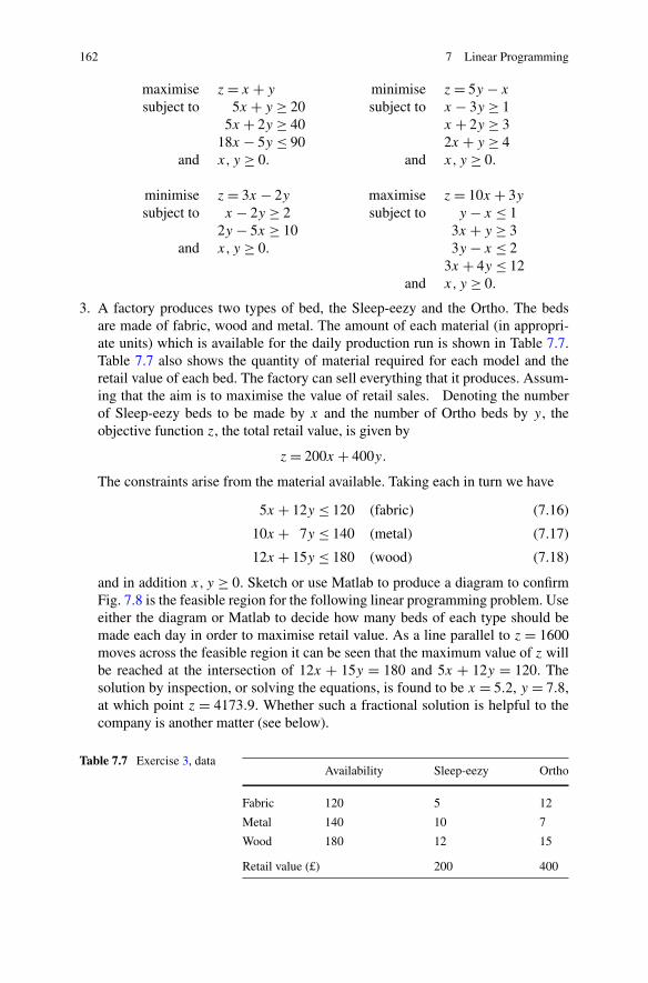
162 7 Linear Programming
maximise z = x + y minimise z = 5y − x
subject to 5x + y ≥ 20 subject to x − 3y ≥ 15x + 2y ≥ 40 x + 2y ≥ 3
18x − 5y ≤ 90 2x + y ≥ 4and x, y ≥ 0. and x, y ≥ 0.
minimise z = 3x − 2y maximise z = 10x + 3y
subject to x − 2y ≥ 2 subject to y − x ≤ 12y − 5x ≥ 10 3x + y ≥ 3
and x, y ≥ 0. 3y − x ≤ 23x + 4y ≤ 12
and x, y ≥ 0.
3. A factory produces two types of bed, the Sleep-eezy and the Ortho. The bedsare made of fabric, wood and metal. The amount of each material (in appropri-ate units) which is available for the daily production run is shown in Table 7.7.Table 7.7 also shows the quantity of material required for each model and theretail value of each bed. The factory can sell everything that it produces. Assum-ing that the aim is to maximise the value of retail sales. Denoting the numberof Sleep-eezy beds to be made by x and the number of Ortho beds by y, theobjective function z, the total retail value, is given by
z = 200x + 400y.
The constraints arise from the material available. Taking each in turn we have
5x + 12y ≤ 120 (fabric) (7.16)
10x + 7y ≤ 140 (metal) (7.17)
12x + 15y ≤ 180 (wood) (7.18)
and in addition x, y ≥ 0. Sketch or use Matlab to produce a diagram to confirmFig. 7.8 is the feasible region for the following linear programming problem. Useeither the diagram or Matlab to decide how many beds of each type should bemade each day in order to maximise retail value. As a line parallel to z = 1600moves across the feasible region it can be seen that the maximum value of z willbe reached at the intersection of 12x + 15y = 180 and 5x + 12y = 120. Thesolution by inspection, or solving the equations, is found to be x = 5.2, y = 7.8,at which point z = 4173.9. Whether such a fractional solution is helpful to thecompany is another matter (see below).
Table 7.7 Exercise 3, dataAvailability Sleep-eezy Ortho
Fabric 120 5 12
Metal 140 10 7
Wood 180 12 15
Retail value (£) 200 400
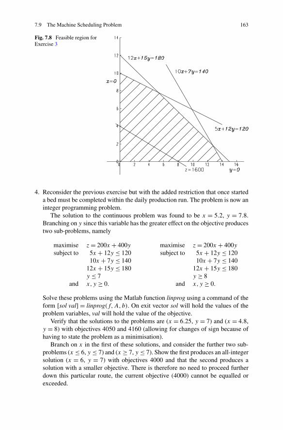
7.9 The Machine Scheduling Problem 163
Fig. 7.8 Feasible region forExercise 3
4. Reconsider the previous exercise but with the added restriction that once starteda bed must be completed within the daily production run. The problem is now aninteger programming problem.
The solution to the continuous problem was found to be x = 5.2, y = 7.8.Branching on y since this variable has the greater effect on the objective producestwo sub-problems, namely
maximise z = 200x + 400y maximise z = 200x + 400y
subject to 5x + 12y ≤ 120 subject to 5x + 12y ≤ 12010x + 7y ≤ 140 10x + 7y ≤ 140
12x + 15y ≤ 180 12x + 15y ≤ 180y ≤ 7 y ≥ 8
and x, y ≥ 0. and x, y ≥ 0.
Solve these problems using the Matlab function linprog using a command of theform [sol val] = linprog(f,A,b). On exit vector sol will hold the values of theproblem variables, val will hold the value of the objective.
Verify that the solutions to the problems are (x = 6.25, y = 7) and (x = 4.8,y = 8) with objectives 4050 and 4160 (allowing for changes of sign because ofhaving to state the problem as a minimisation).
Branch on x in the first of these solutions, and consider the further two sub-problems (x ≤ 6, y ≤ 7) and (x ≥ 7, y ≤ 7). Show the first produces an all-integersolution (x = 6, y = 7) with objectives 4000 and that the second produces asolution with a smaller objective. There is therefore no need to proceed furtherdown this particular route, the current objective (4000) cannot be equalled orexceeded.
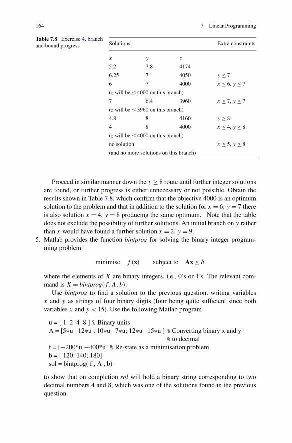
164 7 Linear Programming
Table 7.8 Exercise 4, branchand bound progress Solutions Extra constraints
x y z
5.2 7.8 4174
6.25 7 4050 y ≤ 7
6 7 4000 x ≤ 6, y ≤ 7
(z will be ≤ 4000 on this branch)
7 6.4 3960 x ≥ 7, y ≤ 7
(z will be ≤ 3960 on this branch)
4.8 8 4160 y ≥ 8
4 8 4000 x ≤ 4, y ≥ 8
(z will be ≤ 4000 on this branch)
no solution x ≥ 5, y ≥ 8
(and no more solutions on this branch)
Proceed in similar manner down the y ≥ 8 route until further integer solutionsare found, or further progress is either unnecessary or not possible. Obtain theresults shown in Table 7.8, which confirm that the objective 4000 is an optimumsolution to the problem and that in addition to the solution for x = 6, y = 7 thereis also solution x = 4, y = 8 producing the same optimum. Note that the tabledoes not exclude the possibility of further solutions. An initial branch on y ratherthan x would have found a further solution x = 2, y = 9.
5. Matlab provides the function bintprog for solving the binary integer program-ming problem
minimise f (x) subject to Ax ≤ b
where the elements of X are binary integers, i.e., 0’s or 1’s. The relevant com-mand is X = bintprog(f,A,b).
Use bintprog to find a solution to the previous question, writing variablesx and y as strings of four binary digits (four being quite sufficient since bothvariables x and y < 15). Use the following Matlab program
u = [ 1 2 4 8 ] % Binary unitsA = [5∗u 12∗u ; 10∗u 7∗u; 12∗u 15∗u ] % Converting binary x and y
% to decimalf = [−200*u −400*u] % Re-state as a minimisation problemb = [ 120: 140; 180]sol = bintprog( f , A , b)
to show that on completion sol will hold a binary string corresponding to twodecimal numbers 4 and 8, which was one of the solutions found in the previousquestion.
7.9 The Machine Scheduling Problem 165
6. The all-slack solution to the following linear programming problem is not feasi-ble, since setting the problem variables contravenes the constraints.
minimise z = 3x2 − x1 − 4x3subject to 2x1 + 4x3 ≤ 4
x1 + x2 + x3 = 32x2 − x3 ≥ 2
and x1, x2, x3 ≥ 0.
However by writing the problem in canonical form and introducing slack vari-ables x4, x6 and an artificial variable x5 a basic feasible solution may be foundwith which to start the simplex method. We have
2x1 + 4x3 + x4 = 4
x1 + x2 + x3 + x5 = 3
−2x2 + x3 + x6 = −2
x5 = 0
x1, x2, x3, x4, x6 ≥ 0.
Setting the problem variables (x1, x2, x3) to zero produces x4 = 4, x5 = 3 andx6 = −2 which contravenes the constraints. In order to reduce x5 (to zero) andincrease x6 (to a non-negative value) minimise the pseudo objective z = x5 − x6.The Matlab function linprog has an extended form X = linprog(f, A, b, Aeq, beq)which as before uses A and b for the ≤ constraints and a second pair Aeq , beq forthe equality constraints. Use the following sequence to find a feasible solution.
% equality constraintsAequals = [ 2 0 4 1 0 0; 1 1 1 0 1 0; 0 −2 1 0 0 1; 0 0 0 0 1 0 ]equals = [ 4 3 −2 0 ]% inequality constraints, all ≥ 0 except x(5)A = eye(6); % eye returns a unit diagonal matrix, in this case 6 × 6A = −A; A( 5, 5 ) = 0b = zeros(6,1) % zeros returns a zero matrix, in this case 6 rows, 1 columns% objective, minimise x(5) − x(6)f = [ 0 0 0 0 1 −1 ]X = linprog(f, A, b, Aequals, equals)
7. Consider once again the bed-making factory of Exercise 4. Following marketsurveys the factory is considering switching production from its Ortho model toa new Rest-Rite model. Whereas the material figures for Ortho were 12, 7 and 15,the corresponding figures for the Rest-Rite are 12 (unchanged), 16 and 10, andthe retail value is £550. Assuming that it is not feasible to make incomplete bedsthe decision whether or not to switch production can be modelled as follows:
Let d be the decision variable defined by
d = 1 : switch from Ortho to Rest-Rite
d = 0 : stay with Ortho.
166 7 Linear Programming
Let x1 denote the number of Sleep-eezy beds to be made, x2 the number ofOrtho beds, x3 the number of Rest-Rite beds and let z denote total retail value.The linear programming problem becomes
maximise z = 200x1 + 400x2 + 450x3subject to 5x1 + 12x2 + 12x3 ≤ 120
10x1 + 7x2 + 16x3 ≤ 14012x1 + 15x2 + 10x3 ≤ 180
x2 ≤ 16(1 − d)
x3 ≤ 16d
d ≤ 1x1, x2, x3, d ≥ 0, x1, x2, x3, d integer.
The number 16 is chosen as being larger than any possible value of the problemvariables. Solve the problem using bintprog as explained in question 5 and illus-trated below. Use a Matlab program of similar form, to that shown below. Notingthat the decision variable d is already in single digit binary form, represent eachof the problem variables, x1, x2 and x3 as strings of four binary digits.
u = [ 1 2 4 8 ];% Use the continuation mark . . . for multi-line inputA = [ 5*u 12*u 12*u 0; 10*u 7*u 16*u 0; 12*u 15*u 10*u 0; . . .
0*u 1*u 0*u 16; 0*u 0*u 1*u −16 ];b = [ 120; 140; 180; 16; 0 ];f = [ −200*u −400*u −550*u 0 ];x = bintprog( f, A, b )
Deduce that the factory should make the switch and that retail value may beincreased by £600.
8. Use bintprog to solve the car hire company problem discussed in the problem ofSect. 7.7. In this example all the variables are binary and so there is no need forcoversions to and from decimal. You may find the d1 = 1, d2 = 1, d3 = 0, d4 = 0,d5 = 1, d6 = 0, indicating that models 3, 4 and 6 are no longer required. In thisexample there are three other solutions, which could be found on the branch andbound tree.
9. Use bintprog to solve the travelling salesman problem of Sect. 7.7. The problemhas 25 variables dij which may be represented by a single vector in which thevariables are held in the order
d1,1, d1,2, . . . , d1,5, d2,1, d2,2, . . . , d2,5, d3,1, . . .
The problem as stated has no inequality constraints, the absence of which maybe indicated by entries [ ] in the appropriate positions in the extended parameterlist of bintprog. Typically a command would be of the form
[X value] = bintprog( z, [ ], [ ], A, b );
which returns the solution variables in X and the value of the objective z at thesolution in value. In this example the matrix of constraints has 10 rows and 25
7.9 The Machine Scheduling Problem 167
columns. The task of entering all 250 entries in A may be simplified by not-ing that vector entries may be used to enter a particular sequence of values, butwhichever way is chosen the task of entering the data correctly is not to be underestimated.
You may find that the program produces the solution
d12 = 1, d21 = 1, d35 = 1, d43 = 1, d54 = 1
which represents Manchester–Leeds–Manchester, and in a separate loop, Stoke–Preston–Liverpool–Stoke. Clearly this is not acceptable and so we re-solve theproblem with the added (inequality) constraint
d13 + d14 + d15 + d23 + d24 + d25 ≥ 1
which has the effect of forcing at least one direct link between Manchester orLeeds and Stoke, Liverpool or Preston.
This added constraint produces a solution
d12 = 1, d25 = 1, d31 = 1, d43 = 1, d54 = 1
which either way round is an optimal route, namely Manchester–Leeds–Preston–Liverpool–Stoke–Manchester, a total distance of 250 miles.
Chapter 8Optimisation
Aims In this chapter we look at methods for finding the maximum (or minimum)of a function of one or more variables, possibly subject to constraints. In so doingwe generalise the linear problems of Chap. 7.
In particular we
• explain how we can regard the problem as one of minimisation.• distinguish between local and global minima.• describe the simple grid search and the golden section search methods for func-
tions of a single variable.• describe the method of steepest descent and a rank-one method for unconstrained
problems involving functions of several variables.• describe penalty function methods for constrained problems.
Overview Optimisation is concerned with finding a local maximum or minimumof a function of several variables f (x) ≡ f (x1, x2, . . . , xn). We examine methodsfor both unconstrained problems, in which the independent variables are free totake any values, and constrained problems in which the independent variables areconstrained in some manner. We may have simple bounds such as 0 ≤ x1 ≤ 1 andx2 ≥ 4, linear constraints as in linear programming problems, or more complicatednonlinear constraints such as x2
1 +x2 ≤ 1.5, where x1 and x2 are independent vari-ables. Unlike the linear problems of Chap. 7 it is not possible to give all embracingmethods with guarantees to solve a wide class of problems. The general problemwe investigate in this chapter is altogether more complex and for this reason weapproach the topic by describing methods for
• unconstrained problems• constrained problems.• methods for functions of a single variable• methods for functions of several variables.
Acquired Skills After reading this chapter and completing the exercises you willbe able to
C. Woodford, C. Phillips, Numerical Methods with Worked Examples: Matlab Edition,DOI 10.1007/978-94-007-1366-6_8, © Springer Science+Business Media B.V. 2012
169

170 8 Optimisation
• formulate an optimisation problem as a minimisation problem.• decide when to use and how to apply the grid search and golden section search
methods.• decide when to use and how to apply the method of steepest descent and a rank-
one method, and have some idea as to how a rank-two method might be formu-lated.
• understand what is meant by a penalty function.• find the Lagrangian of a constrained problem.• use the multiplier penalty function method on a Lagrangian to find a solution to a
constrained problem.
8.1 Introduction
Although we look at methods for finding optimal values we simplify the discussionby assuming that we are trying to find minimum, as opposed to maximum, values.This is the opposite situation to linear programming, where unless otherwise statedit is assumed that we are aiming to find a maximum. However, by the reasoninggiven in the overview of Chap. 7 neither case is restrictive since if we are requiredto find the maximum value of a function f , we can do so by finding the minimumvalue of −f and vice versa.
Consideration of what we mean by a local minimum and a global minimumleads to the distinction between a local minimum as a minimum with respect toa local region, whereas a global minimum is the minimum of all local minima.The methods we describe will only provide a local minimum. To decide if such aminimum is a global minimum is a separate issue. In practice we look for clues in thegeneral shape of the function. Figure 8.1 shows a function, f (x) of a single variable
Fig. 8.1 Local and globalminima
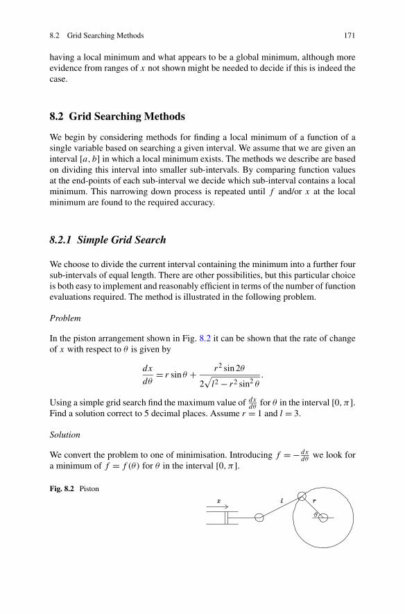
8.2 Grid Searching Methods 171
having a local minimum and what appears to be a global minimum, although moreevidence from ranges of x not shown might be needed to decide if this is indeed thecase.
8.2 Grid Searching Methods
We begin by considering methods for finding a local minimum of a function of asingle variable based on searching a given interval. We assume that we are given aninterval [a, b] in which a local minimum exists. The methods we describe are basedon dividing this interval into smaller sub-intervals. By comparing function valuesat the end-points of each sub-interval we decide which sub-interval contains a localminimum. This narrowing down process is repeated until f and/or x at the localminimum are found to the required accuracy.
8.2.1 Simple Grid Search
We choose to divide the current interval containing the minimum into a further foursub-intervals of equal length. There are other possibilities, but this particular choiceis both easy to implement and reasonably efficient in terms of the number of functionevaluations required. The method is illustrated in the following problem.
Problem
In the piston arrangement shown in Fig. 8.2 it can be shown that the rate of changeof x with respect to θ is given by
dx
dθ= r sin θ + r2 sin 2θ
2√
l2 − r2 sin2 θ.
Using a simple grid search find the maximum value of dxdθ
for θ in the interval [0,π].Find a solution correct to 5 decimal places. Assume r = 1 and l = 3.
Solution
We convert the problem to one of minimisation. Introducing f = − dxdθ
we look fora minimum of f = f (θ) for θ in the interval [0,π].
Fig. 8.2 Piston
172 8 Optimisation
Evaluating f at five equally-spaced points in the interval [0,π] including the endpoints, we have
θ 0 0.78540 1.57080 2.35619 3.14159f (θ) 0 −0.87861 −1 −0.53561 0
The interval containing a minimum can be reduced to [0.78540,2.35619]. Perform-ing a further sub-division we have
θ 0.78540 1.17810 1.57080 1.96350 2.35619f (θ) −0.87861 −1.04775 −1 −0.80001 −0.53561
Note that this second step just involves two new function evaluations, since we al-ready have f (θ) at the two end points and at the middle point θ = 1.57080. Theinterval can now be reduced to [0.78540,1.57080], from which another set of eval-uations produces
θ 0.78540 0.98175 1.17810 1.37445 1.57080f (θ) −0.87861 −0.99173 −1.04775 −1.04827 −1
Proceeding in this way, after a further 6 iterations we obtain
θ 1.27014 1.27320 1.27627 1.27934 1.28241f (θ) −1.05461 −1.05463 −1.05464 −1.05464 −1.05462
indicating that f has a local minimum of −1.05464 (to 5 decimal places) at somepoint in the interval [1.27320,1.27934].
It so happens that in this example the values of the function are the first to con-verge to the required accuracy. To pinpoint the position of the minimum to a similaraccuracy we continue to narrow the interval. Following a further 9 iterations we find
θ 1.27715 1.27715 1.27715 1.27715 1.27715f (θ) −1.05464 −1.05464 −1.05464 −1.05464 −1.05464
indicating that the local minimum is at θ = 1.27715 (to 5 decimal places). In con-clusion, we have dx
dθreaching a maximum value of 1.05464 for θ = 1.27715, (ap-
proximately 73°).
Discussion
The details of the simple grid search are specified in Table 8.1. The method is notdissimilar to the bisection method of Chap. 3 in which we also successively halve theinterval at each step. In the grid search the interval containing the local minimum ishalved after 2 function evaluations. However we can do better than this. In real timeapplications in which the function is time consuming to evaluate such considerationscan be important.
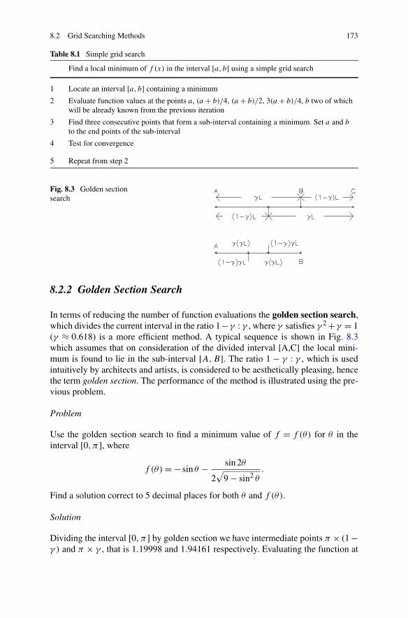
8.2 Grid Searching Methods 173
Table 8.1 Simple grid search
Find a local minimum of f (x) in the interval [a, b] using a simple grid search
1 Locate an interval [a, b] containing a minimum
2 Evaluate function values at the points a, (a + b)/4, (a + b)/2, 3(a + b)/4, b two of whichwill be already known from the previous iteration
3 Find three consecutive points that form a sub-interval containing a minimum. Set a and b
to the end points of the sub-interval
4 Test for convergence
5 Repeat from step 2
Fig. 8.3 Golden sectionsearch
8.2.2 Golden Section Search
In terms of reducing the number of function evaluations the golden section search,which divides the current interval in the ratio 1−γ : γ , where γ satisfies γ 2 +γ = 1(γ ≈ 0.618) is a more efficient method. A typical sequence is shown in Fig. 8.3which assumes that on consideration of the divided interval [A,C] the local mini-mum is found to lie in the sub-interval [A,B]. The ratio 1 − γ : γ , which is usedintuitively by architects and artists, is considered to be aesthetically pleasing, hencethe term golden section. The performance of the method is illustrated using the pre-vious problem.
Problem
Use the golden section search to find a minimum value of f = f (θ) for θ in theinterval [0,π], where
f (θ) = − sin θ − sin 2θ
2√
9 − sin2 θ.
Find a solution correct to 5 decimal places for both θ and f (θ).
Solution
Dividing the interval [0,π] by golden section we have intermediate points π × (1 −γ ) and π × γ , that is 1.19998 and 1.94161 respectively. Evaluating the function at
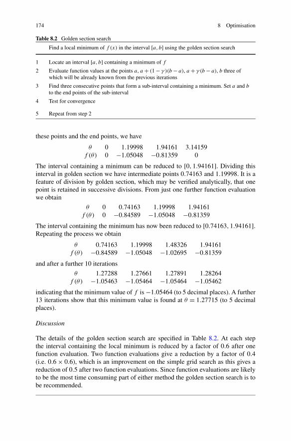
174 8 Optimisation
Table 8.2 Golden section search
Find a local minimum of f (x) in the interval [a, b] using the golden section search
1 Locate an interval [a, b] containing a minimum of f
2 Evaluate function values at the points a, a + (1 − γ )(b − a), a + γ (b − a), b three ofwhich will be already known from the previous iterations
3 Find three consecutive points that form a sub-interval containing a minimum. Set a and b
to the end points of the sub-interval
4 Test for convergence
5 Repeat from step 2
these points and the end points, we have
θ 0 1.19998 1.94161 3.14159f (θ) 0 −1.05048 −0.81359 0
The interval containing a minimum can be reduced to [0,1.94161]. Dividing thisinterval in golden section we have intermediate points 0.74163 and 1.19998. It is afeature of division by golden section, which may be verified analytically, that onepoint is retained in successive divisions. From just one further function evaluationwe obtain
θ 0 0.74163 1.19998 1.94161f (θ) 0 −0.84589 −1.05048 −0.81359
The interval containing the minimum has now been reduced to [0.74163,1.94161].Repeating the process we obtain
θ 0.74163 1.19998 1.48326 1.94161f (θ) −0.84589 −1.05048 −1.02695 −0.81359
and after a further 10 iterations
θ 1.27288 1.27661 1.27891 1.28264f (θ) −1.05463 −1.05464 −1.05464 −1.05462
indicating that the minimum value of f is −1.05464 (to 5 decimal places). A further13 iterations show that this minimum value is found at θ = 1.27715 (to 5 decimalplaces).
Discussion
The details of the golden section search are specified in Table 8.2. At each stepthe interval containing the local minimum is reduced by a factor of 0.6 after onefunction evaluation. Two function evaluations give a reduction by a factor of 0.4(i.e. 0.6 × 0.6), which is an improvement on the simple grid search as this gives areduction of 0.5 after two function evaluations. Since function evaluations are likelyto be the most time consuming part of either method the golden section search is tobe recommended.
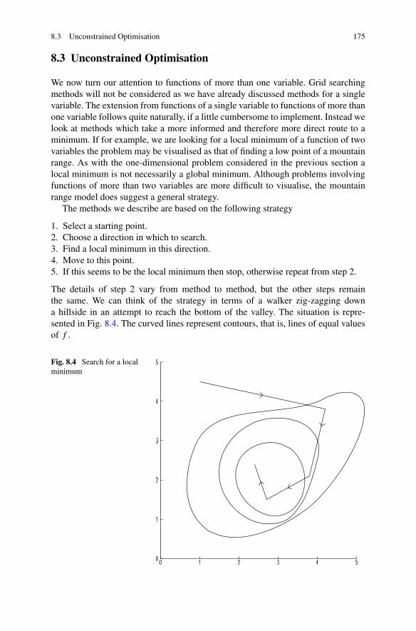
8.3 Unconstrained Optimisation 175
8.3 Unconstrained Optimisation
We now turn our attention to functions of more than one variable. Grid searchingmethods will not be considered as we have already discussed methods for a singlevariable. The extension from functions of a single variable to functions of more thanone variable follows quite naturally, if a little cumbersome to implement. Instead welook at methods which take a more informed and therefore more direct route to aminimum. If for example, we are looking for a local minimum of a function of twovariables the problem may be visualised as that of finding a low point of a mountainrange. As with the one-dimensional problem considered in the previous section alocal minimum is not necessarily a global minimum. Although problems involvingfunctions of more than two variables are more difficult to visualise, the mountainrange model does suggest a general strategy.
The methods we describe are based on the following strategy
1. Select a starting point.2. Choose a direction in which to search.3. Find a local minimum in this direction.4. Move to this point.5. If this seems to be the local minimum then stop, otherwise repeat from step 2.
The details of step 2 vary from method to method, but the other steps remainthe same. We can think of the strategy in terms of a walker zig-zagging downa hillside in an attempt to reach the bottom of the valley. The situation is repre-sented in Fig. 8.4. The curved lines represent contours, that is, lines of equal valuesof f .
Fig. 8.4 Search for a localminimum
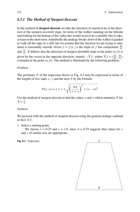
176 8 Optimisation
8.3.1 The Method of Steepest Descent
In the method of steepest descent we take the direction of search to be in the direc-tion of the steepest downhill slope. In terms of the walker standing on the hillsideand looking for the bottom of the valley this would seem to be a sensible line to take,at least in the short term. Admittedly the analogy breaks down if the walker is guidedto walk off the edge of a cliff, but we assume that the function we are trying to min-imise is reasonably smooth. Given f = f (x, y) the slope of f has components ∂f
∂x
and ∂f∂y
. It follows that the direction of steepest downhill slope at the point (a, b) is
given by the vector in the opposite direction, namely −∇f , where ∇f = (∂f∂x
,∂f∂y
)
evaluated at the point (a, b). The method is illustrated by the following problem.
Problem
The perimeter P of the trapezium shown in Fig. 8.5 may be expressed in terms ofthe lengths of two sides x, y and the area A by the formula
P(x, y) = x + y +√(
4A
x + y
)2
+ (y − x)2.
Use the method of steepest descent to find the values x and y which minimise P forA = 1
4 .
Solution
We proceed with the method of steepest descent using the general strategy outlinedin Sect. 8.3.
1. Select a starting point.We choose x = 0.25 and y = 1.0, since A = 0.25 suggests that values for x
and y of similar size are appropriate.
Fig. 8.5 Trapezium
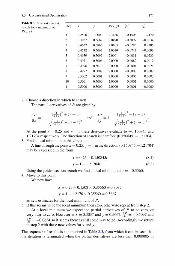
8.3 Unconstrained Optimisation 177
Table 8.3 Steepest descentsearch for a minimum ofP (x, y)
Step x y P (x, y) ∂P∂x
∂P∂y
1 0.2500 1.0000 2.3466 −0.1508 1.2170
2 0.3037 0.5667 2.0490 −0.5097 −0.0634
3 0.4632 0.5866 2.0103 −0.0285 0.2285
4 0.4732 0.5062 2.0010 −0.0743 −0.0096
5 0.4959 0.5092 2.0001 −0.0031 0.0235
6 0.4971 0.5006 2.0000 −0.0082 −0.0012
7 0.4996 0.5010 2.0000 −0.0004 0.0024
8 0.4997 0.5002 2.0000 −0.0008 0.0002
9 0.5002 0.5001 2.0000 0.0006 0.0003
10 0.5001 0.5000 2.0000 0.0002 0.0000
11 0.5000 0.5000 2.0000 0.0001 −0.0000
2. Choose a direction in which to search.The partial derivatives of P are given by
∂P
∂x= 1 − ( 1
x+y)3 + (y − x)
√( 1x+y
)2 + (y − x)2and
∂P
∂y= 1 − ( 1
x+y)3 − (y − x)
√( 1x+y
)2 + (y − x)2.
At the point x = 0.25 and y = 1 these derivatives evaluate to −0.150845 and1.21704 respectively. The direction of search is therefore (0.150845,−1.21704).
3. Find a local minimum in this direction.A line through the point x = 0.25, y = 1 in the direction (0.150845,−1.21704)
may be expressed in the form
x = 0.25 + 0.150845t (8.1)
y = 1 − 1.21704t. (8.2)
Using the golden section search we find a local minimum at t = −0.3560.4. Move to this point
We now have
x = 0.25 + 0.1508 × 0.35560 = 0.3037
y = 1 − 1.2170 × 0.35560 = 0.5667
as new estimates for the local minimum of P .5. If this seems to be the local minimum then stop, otherwise repeat from step 2.
At a local minimum we expect the partial derivatives of P to be zero, orvery near to zero. However at x = 0.3037 and y = 0.5667, ∂P
∂x= −0.5097 and
∂P∂y
= −0.0634 so it seems there is still some way to go. Accordingly we returnto step 2 with these new values for x and y.
The sequence of results is summarised in Table 8.3, from which it can be seen thatthe iteration is terminated when the partial derivatives are less than 0.000005 in
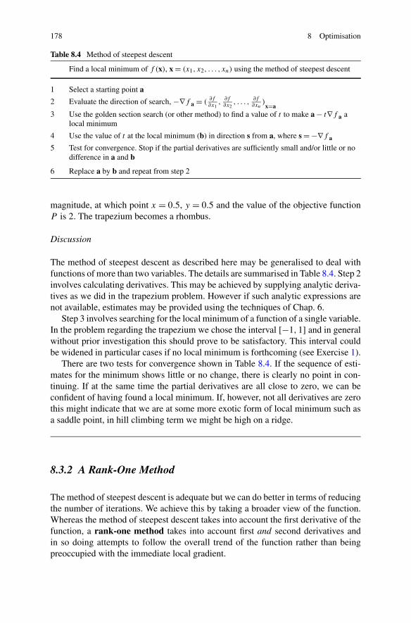
178 8 Optimisation
Table 8.4 Method of steepest descent
Find a local minimum of f (x), x = (x1, x2, . . . , xn) using the method of steepest descent
1 Select a starting point a
2 Evaluate the direction of search, −∇f a = (∂f∂x1
,∂f∂x2
, . . . ,∂f∂xn
)x=a
3 Use the golden section search (or other method) to find a value of t to make a − t∇f a alocal minimum
4 Use the value of t at the local minimum (b) in direction s from a, where s = −∇f a
5 Test for convergence. Stop if the partial derivatives are sufficiently small and/or little or nodifference in a and b
6 Replace a by b and repeat from step 2
magnitude, at which point x = 0.5, y = 0.5 and the value of the objective functionP is 2. The trapezium becomes a rhombus.
Discussion
The method of steepest descent as described here may be generalised to deal withfunctions of more than two variables. The details are summarised in Table 8.4. Step 2involves calculating derivatives. This may be achieved by supplying analytic deriva-tives as we did in the trapezium problem. However if such analytic expressions arenot available, estimates may be provided using the techniques of Chap. 6.
Step 3 involves searching for the local minimum of a function of a single variable.In the problem regarding the trapezium we chose the interval [−1,1] and in generalwithout prior investigation this should prove to be satisfactory. This interval couldbe widened in particular cases if no local minimum is forthcoming (see Exercise 1).
There are two tests for convergence shown in Table 8.4. If the sequence of esti-mates for the minimum shows little or no change, there is clearly no point in con-tinuing. If at the same time the partial derivatives are all close to zero, we can beconfident of having found a local minimum. If, however, not all derivatives are zerothis might indicate that we are at some more exotic form of local minimum such asa saddle point, in hill climbing term we might be high on a ridge.
8.3.2 A Rank-One Method
The method of steepest descent is adequate but we can do better in terms of reducingthe number of iterations. We achieve this by taking a broader view of the function.Whereas the method of steepest descent takes into account the first derivative of thefunction, a rank-one method takes into account first and second derivatives andin so doing attempts to follow the overall trend of the function rather than beingpreoccupied with the immediate local gradient.
8.3 Unconstrained Optimisation 179
We assume that we are at the point x = a, y = b in our search for a localminimum of the function f = f (x, y) and that in accordance with the strategy ofSect. 8.3 we search for a local minimum in the as yet unspecified direction (s1, s2).Using (8.1) and (8.2) as the model we write
x = a + ts1
y = b + ts2
in a Taylor series expansion of f (x, y). For sufficiently small t we have
f (a + ts1, b + ts2) = f (a, b) + t
(s1
∂f
∂x+ s2
∂f
∂y
)
+ t2
2
(s2
1∂2f
∂x2+ 2s1s2
∂2f
∂x∂y+ s2
2∂2f
∂y2
)+ higher order terms
where all derivatives are evaluated at x = a, y = b. Our aim is to find values x, y
such that f (x, y) is less than f (a, b). If we choose s1 and s2 so that
s1∂2f
∂x2+ s2
∂2f
∂x∂y= −∂f
∂x(8.3)
s1∂2f
∂x∂y+ s2
∂2f
∂y2= −∂f
∂y(8.4)
it follows that
f (x, y) = f (a, b)
+1
2
[(1 − t)2 − 1
](s2
1∂2f
∂x2+ 2s1s2
∂2f
∂x∂y+ s2
2∂2f
∂y2
).
Therefore if |t | < 1 and (s21
∂2f
∂x2 + 2s1s2∂2f∂x∂y
+ s22
∂2f
∂y2 ) > 0 then f (x, y) < f (a, b).It is easy enough to ensure the first of these conditions by not wandering too farfrom the current estimate. The second condition is automatically satisfied at a localminimum, so there is reason to suppose that it will be satisfied if we are not toofar away. Together the conditions suggest that f (x, y) < f (a, b) for (x, y) local to(a, b) and so we have a local minimum.
Problem
Use a rank-one method to find values x and y which minimise P = P(x, y), where
P = x + y +√(
1
x + y
)2
+ (y − x)2.
Solution
This is the problem solved earlier using the method of steepest descent. As withsteepest descent we follow the general strategy of Sect. 8.3.
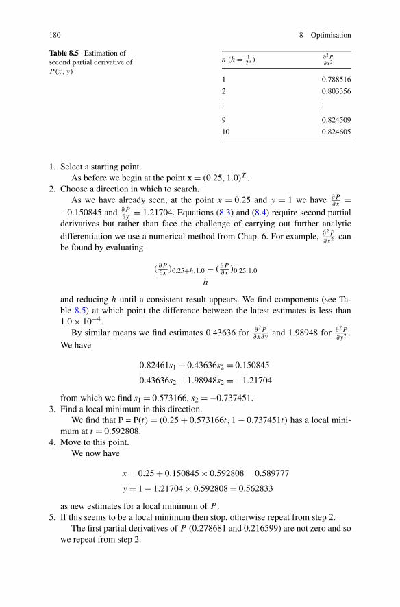
180 8 Optimisation
Table 8.5 Estimation ofsecond partial derivative ofP (x, y)
n (h = 12n ) ∂2P
∂x2
1 0.788516
2 0.803356...
.
.
.
9 0.824509
10 0.824605
1. Select a starting point.As before we begin at the point x = (0.25,1.0)T .
2. Choose a direction in which to search.As we have already seen, at the point x = 0.25 and y = 1 we have ∂P
∂x=
−0.150845 and ∂P∂y
= 1.21704. Equations (8.3) and (8.4) require second partialderivatives but rather than face the challenge of carrying out further analytic
differentiation we use a numerical method from Chap. 6. For example, ∂2P
∂x2 canbe found by evaluating
( ∂P∂x
)0.25+h,1.0 − ( ∂P∂x
)0.25,1.0
h
and reducing h until a consistent result appears. We find components (see Ta-ble 8.5) at which point the difference between the latest estimates is less than1.0 × 10−4.
By similar means we find estimates 0.43636 for ∂2P∂x∂y
and 1.98948 for ∂2P
∂y2 .We have
0.82461s1 + 0.43636s2 = 0.150845
0.43636s2 + 1.98948s2 = −1.21704
from which we find s1 = 0.573166, s2 = −0.737451.3. Find a local minimum in this direction.
We find that P = P(t) = (0.25 + 0.573166t,1 − 0.737451t) has a local mini-mum at t = 0.592808.
4. Move to this point.We now have
x = 0.25 + 0.150845 × 0.592808 = 0.589777
y = 1 − 1.21704 × 0.592808 = 0.562833
as new estimates for a local minimum of P .5. If this seems to be a local minimum then stop, otherwise repeat from step 2.
The first partial derivatives of P (0.278681 and 0.216599) are not zero and sowe repeat from step 2.

8.3 Unconstrained Optimisation 181
Table 8.6 Rank-one searchfor a minimum of P (x, y)
using a linear equation solver
x y P (x, y) ∂P∂x
∂P∂y
1 0.25000 1.00000 2.34659 −0.15084 1.21704
2 0.58978 0.56283 2.02062 0.27868 0.21660
3 0.50408 0.49539 2.00004 0.00765 −0.00972
4 0.50001 0.50001 2.00000 0.00004 0.00003
5 0.50000 0.50000 2.00000 0.00000 0.00000
The sequence of results is summarised in Table 8.6 from which it can be seen thatthe iteration is terminated when the partial derivatives are zero (to 5 decimal places),at which point x = 0.5, y = 0.5 and the value of the objective function P is 2. Thiscompares with the result obtained by the method of steepest descent.
It is clear that the rank-one method has found the same local minimum of P =P(x, y) in fewer iterations than the method of steepest descent. For most functionsthis is generally the case and so the extra computation involved in the rank-onemethod is deemed to be worthwhile.
8.3.3 Generalised Rank-One Method
Having considered the rank one method for finding a local minimum of a functionof two variables we move on to the general case. We formulate the method and inso doing provide a more economical method. Extending (8.3) and (8.4) to deal withn functions f1, . . . , fn of n variables x1, . . . , xn we have
⎛
⎜⎜⎜⎜⎜⎜⎝
∂2f
∂x21
∂2f∂x1∂x2
∂2f∂x1∂x3
· · ·∂2f
∂x1∂x2
∂2f
∂x22
∂2f∂x2∂x3
· · ·∂2f
∂x1∂x3
∂2f∂x2∂x3
∂2f
∂x23
· · ·...
......
. . .
⎞
⎟⎟⎟⎟⎟⎟⎠
⎛
⎜⎜⎜⎜⎜⎝
s1
s2
s3
...
⎞
⎟⎟⎟⎟⎟⎠
=
⎛
⎜⎜⎜⎜⎜⎝
− ∂f∂x1
− ∂f∂x2
− ∂f∂x3
...
⎞
⎟⎟⎟⎟⎟⎠
.
Writing the above in matrix terms we have
Gs = −∇f .
As an alternative to solving this linear system of equations in order to find the direc-tion of search s we use the approximation
s = −H∇f (8.5)
where H is as yet unspecified, but is chosen in such a way that it may be expectedto converge towards the inverse of G as the search for the local minimum of f
proceeds. This may be an unnecessary complication for a 2×2 system and similarlysmall systems, but if we are dealing with larger systems we replace finding a solution
182 8 Optimisation
Table 8.7 Rank-one method, without a linear equation solver
Find a local minimum of f (x), x = (x1, x2, . . . , xn) using a rank-one method
1 Select a starting point a and let H be the identity matrix
2 Evaluate ∇f a = (∂f∂x1
,∂f∂x2
, . . . ,∂f∂xn
)a
3 Test for convergence, depending on the problem. Stop if the partial derivatives aresufficiently small and/or little or no difference in a and b
4 Search for a local minimum, (b) in direction s from a, where s = −H∇f a
5 Replace H by H + E where E = αuuT ,u = (b − a) − H(∇b − ∇a) andα = 1/(uT (∇b − ∇a)). Replace a by b
6 Repeat from step 2
to a system of tens or perhaps hundreds of linear equations by the simpler matrix–vector multiplication, (8.5).
There are many choices for H, but typically the rank-one method initially sets Hto I, the identity matrix, and with each iteration adds an increment E, where E is amatrix of the form
E = αuuT . (8.6)
The matrix E is said to be of rank-one since it has one linearly independent column(every column is a multiple of any one of the others), hence the name rank-onemethod.
Now for the choice of how H is to be incremented. We recall from Chap. 6that given a function f = f (x) we may make the approximation f ′′(x) = (f ′(b) −f ′(a))/(b − a) for x in the interval [a, b]. This result generalises to functions ofseveral variables to give the approximation
G(b − a) = ∇b − ∇a.
It follows that if we have an estimate a for the minimum and the search directionleads to an estimate b and in so doing H takes a new value H + E we have
(H + E)(b − a) = ∇b − ∇a.
Equating H + E to G−1 we have
b − a = (H + E)(∇b − ∇a)
= (H + αuuT )(∇b − ∇a)
which we can satisfy by choosing α and u so that
u = (b − a) − H(∇b − ∇a) (8.7)
αuT (∇b − ∇a) = 1. (8.8)
We now have our algorithm for updating H at each step of the iteration. The rank-one method is summarised in Table 8.7.
In conclusion we note that although the method works well, particularly if theiteration is started with a good estimate of the solution, it cannot be guaranteed to

8.3 Unconstrained Optimisation 183
converge. A method based on incrementing H by a rank two matrix, E constructedso as to ensure the search for a minimum proceeds in a downhill manner is morelikely to converge.
Problem
Use the generalised rank-one method to find values x and y which minimise P =P(x, y), where
P = x + y +√(
1
x + y
)2
+ (y − x)2.
Solution
This is the problem solved earlier by the method of steepest descent and our firstrank-one method. We use the generalised rank-one method to illustrate how theiteration proceeds without having to solve a set of linear equations at each step.
1. Select a starting point.As before we begin at the point x = (0.25,1.0)T . We take H to be the matrix(
1 00 1
). Since at this stage we have no idea of the value of H at the minimum
point, the choice of the identity matrix would seem to be as good a starting pointas any other.
2. Choose a direction in which to search.As we have already seen, at the point x = 0.25 and y = 1 we have ∂P
∂x=
−0.150845 and ∂P∂y
= 1.21704, and so from (8.5) the search direction s =(s1, s2)
T is given by(
s1s2
)= −
(1 00 1
)(−0.1508451.21704
).
The direction of search is therefore (0.150845,−1.21704)T , which, given theparticular starting choice for H, is the same as for steepest descent.
3. Find a local minimum in this direction.As before we find that P (0.25 + 0.150845t,1 − 1.21704t) has a local mini-
mum at t = 0.355955.4. Move to this point.
We now have
x = 0.25 + 0.150845 × 0.355955 = 0.303694
y = 1 − 1.21704 × 0.355955 = 0.566789
as new estimates for a local minimum of P .5. If this seems to be a local minimum then stop, otherwise repeat from step 2.
The partial derivatives of P (−0.50965 and −0.06317) are not zero and sowe repeat from step 2 after completing the following step
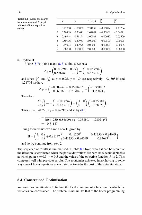
184 8 Optimisation
Table 8.8 Rank-one searchfor a minimum of P (x, y)
without a linear equationsolver
x y P (x, y) ∂P∂x
∂P∂y
1 0.25000 1.00000 2.34659 −0.15084 1.21704
2 0.30369 0.56681 2.04901 −0.50961 −0.0608
3 0.49944 0.51194 2.00021 0.00982 0.03509
4 0.50176 0.49973 2.00000 0.00500 0.00095
5 0.49994 0.49998 2.00000 −0.00001 0.00005
6 0.50000 0.50000 2.00000 0.00000 0.00000
6. Update HUsing (8.7) to find u and (8.8) to find α we have
�x =(
0.303694 − 0.250.566789 − 1.0
)=
(0.053694
−0.433211
)
and since ∂P∂x
and ∂P∂y
at x = 0.25, y = 1.0 are respectively −0.150845 and1.21704 we have
�f ′ =(−0.509648 + 0.150845
−0.063168 − 1.21704
)=
(−0.35880−1.28021
).
Therefore(
u1u2
)= −
(0.053694
−0.433211
)−
(1 00 1
)(−0.35880−1.28021
).
Thus u1 = 0.41250, u2 = 0.84699, and so by (8.8)
α = 1
[(0.41250,0.84699) ∗ (−0.35880,−1.28021)T ]= −0.81147.
Using these values we have a new H given by
H =(
1 00 1
)+ 0.81147
(0.412502 0.41250 × 0.84699
0.41250 × 0.84699 0.846992
)
and so we continue from step 2.
The sequence of results is summarised in Table 8.8 from which it can be seen thatthe iteration is terminated when the partial derivatives are zero (to 5 decimal places)at which point x = 0.5, y = 0.5 and the value of the objective function P is 2. Thiscompares well with previous results. The economies achieved in not having to solvea system of linear equations at each step outweighs the cost of the extra iteration.
8.4 Constrained Optimisation
We now turn our attention to finding the local minimum of a function for which thevariables are constrained. The problem is not unlike that of the linear programming
8.4 Constrained Optimisation 185
of Chap. 7 although we now expect to deal with a nonlinear objective and allow fornonlinear constraints.
8.4.1 Minimisation by Use of a Simple Penalty Function
We consider a simplification in which the constraints on the objective are all equal-ities. We begin with a problem having just one equality constraint and introduce thepenalty function method. It might be possible in such simple cases to eliminateone of the variables and solve the problem analytically. However, practical prob-lems rarely present themselves in this manner and so we look for a more generalmethod.
Problem
Find a local minimum of f = f (x, y) where
f (x, y) = x2 + xy − 1
subject to
x + y2 − 2 = 0
using a simple penalty function method.
Solution
We solve the problem by finding a local minimum of a new function f = f (x, y)
where
f (x, y) = x2 + xy − 1 + σ(x + y2 − 2
)2.
In this case (x + y2 − 2)2
is referred to as the penalty function since it is a measureof by how much the constraint on the problem is not satisfied. The hope is that inminimising f we will also be minimising the penalty function (to zero). Using therank-one method of Sect. 8.3.2 with starting values x = 1, y = 1 and σ = 1 we findthat f has a local minimum at x = −1.03739, y = 1.78403 and that the value of thepenalty function is 0.02113.
Since the penalty function is not quite zero, we repeat but with a new f (x, y)
defined by
f (x, y) = x2 + xy − 1 + σ(x + y2 − 2
)2, σ = 10,
in the hope that the value of the penalty function at the minimum will be smallerto minimise the effect of the factor 10. This time we find a local minimum at x =−1.01645, y = 1.74099 and that the penalty function has a value of order 10−4. Weare therefore getting close to a zero penalty.
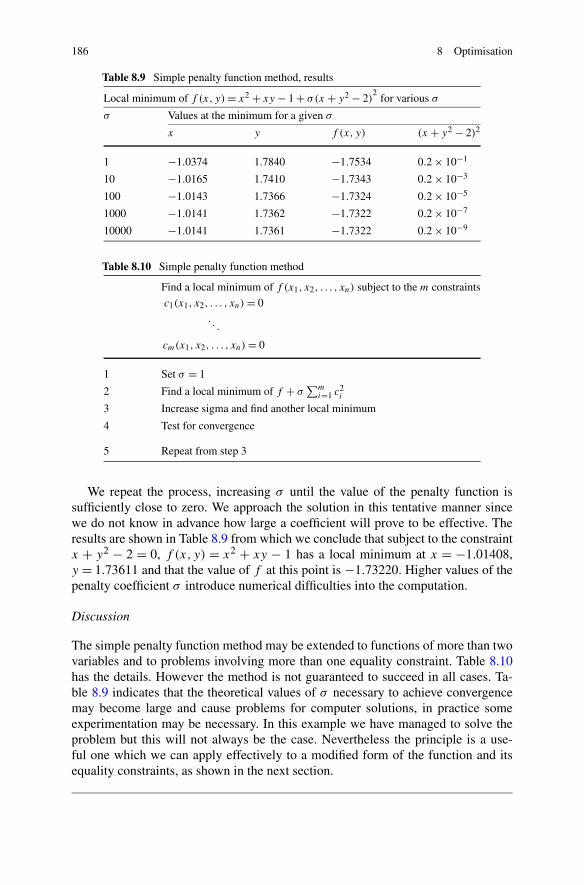
186 8 Optimisation
Table 8.9 Simple penalty function method, results
Local minimum of f (x, y) = x2 + xy − 1 + σ(x + y2 − 2)2
for various σ
σ Values at the minimum for a given σ
x y f (x, y) (x + y2 − 2)2
1 −1.0374 1.7840 −1.7534 0.2 × 10⁻¹
10 −1.0165 1.7410 −1.7343 0.2 × 10⁻³
100 −1.0143 1.7366 −1.7324 0.2 × 10⁻⁵
1000 −1.0141 1.7362 −1.7322 0.2 × 10⁻⁷
10000 −1.0141 1.7361 −1.7322 0.2 × 10⁻⁹
Table 8.10 Simple penalty function method
Find a local minimum of f (x1, x2, . . . , xn) subject to the m constraints
c1(x1, x2, . . . , xn) = 0. . .
cm(x1, x2, . . . , xn) = 0
1 Set σ = 1
2 Find a local minimum of f + σ∑m
i=1 c2i
3 Increase sigma and find another local minimum
4 Test for convergence
5 Repeat from step 3
We repeat the process, increasing σ until the value of the penalty function issufficiently close to zero. We approach the solution in this tentative manner sincewe do not know in advance how large a coefficient will prove to be effective. Theresults are shown in Table 8.9 from which we conclude that subject to the constraintx + y2 − 2 = 0, f (x, y) = x2 + xy − 1 has a local minimum at x = −1.01408,y = 1.73611 and that the value of f at this point is −1.73220. Higher values of thepenalty coefficient σ introduce numerical difficulties into the computation.
Discussion
The simple penalty function method may be extended to functions of more than twovariables and to problems involving more than one equality constraint. Table 8.10has the details. However the method is not guaranteed to succeed in all cases. Ta-ble 8.9 indicates that the theoretical values of σ necessary to achieve convergencemay become large and cause problems for computer solutions, in practice someexperimentation may be necessary. In this example we have managed to solve theproblem but this will not always be the case. Nevertheless the principle is a use-ful one which we can apply effectively to a modified form of the function and itsequality constraints, as shown in the next section.
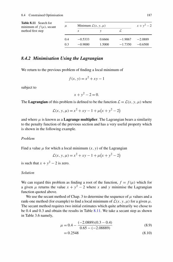
8.4 Constrained Optimisation 187
Table 8.11 Search forminimum of f (μ), secantmethod first step
μ Minimum L(x, y,μ) x + y2 − 2
x y L
0.4 −0.5333 0.6666 −1.9067 −2.0889
0.3 −0.9000 1.5000 −1.7350 −0.6500
8.4.2 Minimisation Using the Lagrangian
We return to the previous problem of finding a local minimum of
f (x, y) = x2 + xy − 1
subject to
x + y2 − 2 = 0.
The Lagrangian of this problem is defined to be the function L = L(x, y,μ) where
L(x, y,μ) = x2 + xy − 1 + μ(x + y2 − 2
)
and where μ is known as a Lagrange multiplier. The Lagrangian bears a similarityto the penalty function of the previous section and has a very useful property whichis shown in the following example.
Problem
Find a value μ for which a local minimum (x, y) of the Lagrangian
L(x, y,μ) = x2 + xy − 1 + μ(x + y2 − 2
)
is such that x + y2 − 2 is zero.
Solution
We can regard this problem as finding a root of the function, f = f (μ) which fora given μ returns the value x + y2 − 2 where x and y minimise the Lagrangianfunction quoted above.
We use the secant method of Chap. 3 to determine the sequence of μ values and arank-one method (for example) to find a local minimum of L(x, y,μ) for a given μ.The secant method requires two initial estimates which quite arbitrarily we chose tobe 0.4 and 0.3 and obtain the results in Table 8.11. We take a secant step as shownin Table 3.6 namely,
μ = 0.4 − (−2.0889)(0.3 − 0.4)
0.65 − (−2.08889)(8.9)
= 0.2548 (8.10)
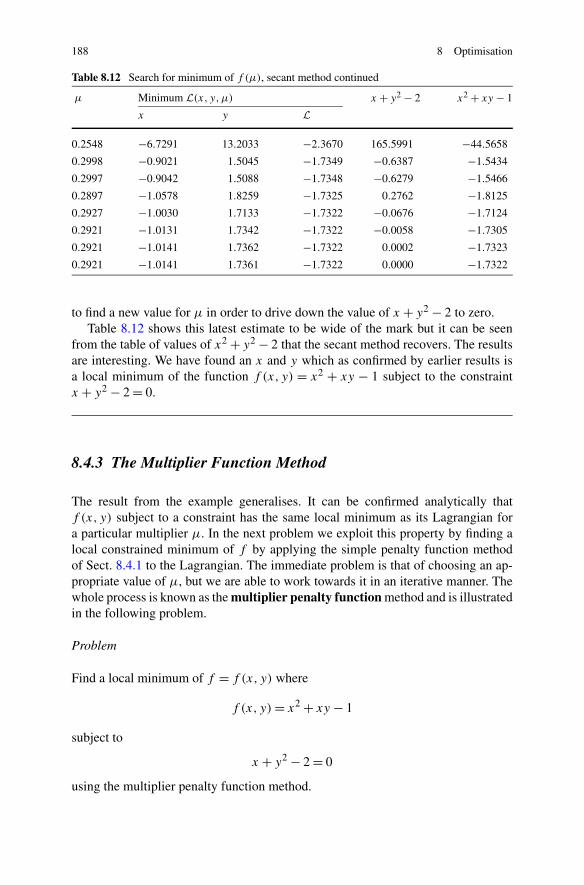
188 8 Optimisation
Table 8.12 Search for minimum of f (μ), secant method continued
μ Minimum L(x, y,μ) x + y2 − 2 x2 + xy − 1
x y L
0.2548 −6.7291 13.2033 −2.3670 165.5991 −44.5658
0.2998 −0.9021 1.5045 −1.7349 −0.6387 −1.5434
0.2997 −0.9042 1.5088 −1.7348 −0.6279 −1.5466
0.2897 −1.0578 1.8259 −1.7325 0.2762 −1.8125
0.2927 −1.0030 1.7133 −1.7322 −0.0676 −1.7124
0.2921 −1.0131 1.7342 −1.7322 −0.0058 −1.7305
0.2921 −1.0141 1.7362 −1.7322 0.0002 −1.7323
0.2921 −1.0141 1.7361 −1.7322 0.0000 −1.7322
to find a new value for μ in order to drive down the value of x + y2 − 2 to zero.Table 8.12 shows this latest estimate to be wide of the mark but it can be seen
from the table of values of x2 + y2 − 2 that the secant method recovers. The resultsare interesting. We have found an x and y which as confirmed by earlier results isa local minimum of the function f (x, y) = x2 + xy − 1 subject to the constraintx + y2 − 2 = 0.
8.4.3 The Multiplier Function Method
The result from the example generalises. It can be confirmed analytically thatf (x, y) subject to a constraint has the same local minimum as its Lagrangian fora particular multiplier μ. In the next problem we exploit this property by finding alocal constrained minimum of f by applying the simple penalty function methodof Sect. 8.4.1 to the Lagrangian. The immediate problem is that of choosing an ap-propriate value of μ, but we are able to work towards it in an iterative manner. Thewhole process is known as the multiplier penalty function method and is illustratedin the following problem.
Problem
Find a local minimum of f = f (x, y) where
f (x, y) = x2 + xy − 1
subject to
x + y2 − 2 = 0
using the multiplier penalty function method.
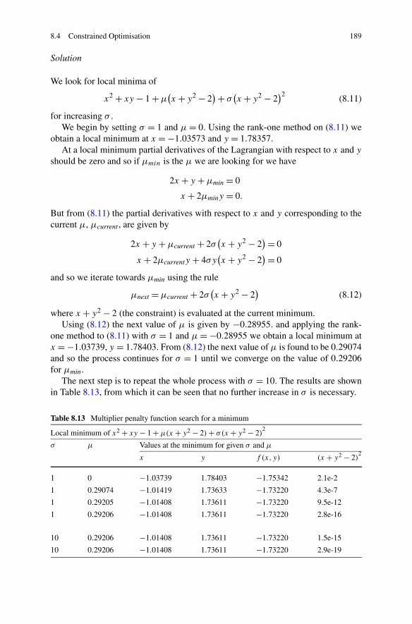
8.4 Constrained Optimisation 189
Solution
We look for local minima of
x2 + xy − 1 + μ(x + y2 − 2
) + σ(x + y2 − 2
)2(8.11)
for increasing σ .We begin by setting σ = 1 and μ = 0. Using the rank-one method on (8.11) we
obtain a local minimum at x = −1.03573 and y = 1.78357.At a local minimum partial derivatives of the Lagrangian with respect to x and y
should be zero and so if μmin is the μ we are looking for we have
2x + y + μmin = 0
x + 2μminy = 0.
But from (8.11) the partial derivatives with respect to x and y corresponding to thecurrent μ, μcurrent, are given by
2x + y + μcurrent + 2σ(x + y2 − 2
) = 0
x + 2μcurrenty + 4σy(x + y2 − 2
) = 0
and so we iterate towards μmin using the rule
μnext = μcurrent + 2σ(x + y2 − 2
)(8.12)
where x + y2 − 2 (the constraint) is evaluated at the current minimum.Using (8.12) the next value of μ is given by −0.28955. and applying the rank-
one method to (8.11) with σ = 1 and μ = −0.28955 we obtain a local minimum atx = −1.03739, y = 1.78403. From (8.12) the next value of μ is found to be 0.29074and so the process continues for σ = 1 until we converge on the value of 0.29206for μmin.
The next step is to repeat the whole process with σ = 10. The results are shownin Table 8.13, from which it can be seen that no further increase in σ is necessary.
Table 8.13 Multiplier penalty function search for a minimum
Local minimum of x2 + xy − 1 + μ(x + y2 − 2) + σ(x + y2 − 2)2
σ μ Values at the minimum for given σ and μ
x y f (x, y) (x + y2 − 2)2
1 0 −1.03739 1.78403 −1.75342 2.1e-2
1 0.29074 −1.01419 1.73633 −1.73220 4.3e-7
1 0.29205 −1.01408 1.73611 −1.73220 9.5e-12
1 0.29206 −1.01408 1.73611 −1.73220 2.8e-16
10 0.29206 −1.01408 1.73611 −1.73220 1.5e-15
10 0.29206 −1.01408 1.73611 −1.73220 2.9e-19

190 8 Optimisation
Table 8.14 Multiplier penalty function method
Find a local minimum of f (x1, x2, . . . , xn) subject to the m constraints
c1(x1, x2, . . . , xn) = 0. . .
cm(x1, x2, . . . , xn) = 0
1 Set σ = 1, μi = 0 (i = 1, . . . ,m)
2 Find a local minimum of f + ∑mi=1 μici + σ
∑mi=1 c2
i
3 Replace μi by μi + 2σci , where the ci are evaluated at the minimum Find another localminimum
4 If the differences between successive minima are not sufficiently small then repeat fromstep 3
5 Increase σ and repeat from step 2
6 If the differences between successive minima are sufficiently small then stop
7 Repeat from step 3
Discussion
The multiplier penalty function method may be extended to functions of more thantwo variables and subject to more than one equality constraint. Table 8.14 has thedetails. The advantage of the method is that it generally avoids the problems of largeσ values which are often found when using the simple penalty function method onthe function to be minimised rather than its Lagrangian. A comparison of Tables 8.9and 8.13 show how the multiplier penalty function method may avoid the problemof having to use very large σ values.
Summary In this chapter we have looked at ways of finding a local minimumof a function of one or more variables possibly subject to constraints. We began byconsidering what is meant by a local minimum and in particular established thatfinding a minimum is essentially the same problem as finding a maximum.
We first considered the simplest problem of all, namely that of finding a localminimum of a function of a single variable for which we used methods based ondividing a given interval. On grounds of efficiency and reliability the golden sectionsearch is the recommended method.
We then moved on to the problem of finding a local minimum of a function ofseveral variables. We established a search strategy within which different choices forthe direction of search give rise to different methods. We considered the method ofsteepest descent and a rank-one method, and whilst advocating the rank-one methodit was realised that a rank-two method might be better. All the methods involverepeated searches in a given direction for which the golden section method is used.
Finally we considered the problem of finding a local minimum of a function ofseveral variables subject to one or more constraints. We showed that it is possible to

8.4 Constrained Optimisation 191
achieve this by means of a simple penalty function although using a penalty functionapplied to the Lagrangian, the so called multiplier penalty function method, is likelyto be more reliable. Whatever the method the problem was solved by reducing theconstrained problem to a series of unconstrained problems for which we had alreadyestablished a rank-one solution method.
Exercises
1. Write a Matlab function with a heading such as
function[pos min] = golden(@f,a, b, eps)
to find the minimum of a function f (specified in an M-file f.m) of a single vari-able in the range [a, b] using the Golden Section Search. The search is to becontinued until the absolute difference of successive approximations to the min-imum position is less than eps. The outputs shown as pos and min are to containthe position of the minimum and its value. An optional third output parametermight be included to signal success or failure to find a minimum. Further op-tions might include parameters to allow function values and relative values tocontrol the iteration. Test the function using examples quoted in the chapter andon examples of your own choosing.
As an added feature arrange for the golden function to extend the range [a, b]by 50% at either the upper or lower end if the function values at a, b and the twointermediate points are in ascending or descending order. In such cases it wouldappear that the function does have a local minimum (or maximum) within thegiven range. This feature will be useful when the golden function is to be used aspart of programs which implement optimisation routines involving line searchesin which the search interval is not predetermined. Assuming an initial searchinterval of [−1,1], allowing for expansion is usually found to be successful.
2. Matlab provides a function fminsearch to find an unconstrained local minimumof a function, starting from a supplied point and continuing within prescribedconvergence criteria until either a satisfactory solution is found or the search isabandoned. Taking default options the following command would find a localminimum of a function f defined in the M-file f.m. using the value stored in thevariable init as the starting point.
[pos min] = fminsearch(@fn, init)
Default options may be overwritten using the optimset function as shown below.
% Termination tolerances for x and f(x) valuesoptions = optimset('TolX',1e-5, 'TolF', 1e-6);[pos min] = fminsearch(@fn, init, options)
Use fminsearch to verify results from the previous question and any of the exam-ples quoted in the chapter.
3. Write a function Pline with parameter t to evaluate the function P given by
P(x, y) = x + y +√(
1
x + y
)2
+ (y − x)2
192 8 Optimisation
for (x, y) values given by x = a + λ1t , y = b + λ2. Make a, b and the λ’s avail-able to Pline by separate global variables (see page 132 or the example below).
Use the function golden (from question 1) with Pline as a parameter to verifythat a line through the point (0.25,1) in the direction (0.15084,−1.21704) findsa local minimum P of 2.0490 for t = −0.3560 and so confirm the result quotedin Table 8.3.
4. Write a program to implement the method of Steepest Descent applied to thefunction, P specified in the previous question with a view to verifying resultsfrom the problem quoted in Table 8.3. Follow the scheme outlined in Table 8.4.The function P should be defined in a separate M-file to return the values of thefunction P(x, y) and its partial derivatives ∂P
∂xand ∂P
∂yfor any (x, y). Use the
function golden with function Pline (from the previous) as a parameter to do theline searches for a minimum position.
% Global variables to be similarly defined in function Plineglobal est grad;
% initial estimate of minimum positionest = [0.25 1];
% loop until the norm (size) of the increment% to the current estimate is sufficiently small
while norm(increment) > 0.1e-5% obtain current function value and partial derivatives
[f grad] = P(est);% monitor progress
s = sprintf('%8.4f ', est, f, grad);disp(s)
% find the minimum along a line through a in direction -grad(a)grad = −grad[tvalue min] = golden (@Pline, −1, 1, 0.1e-7);increment = −tvalue∗grad;est = est + tvalue∗grad;
end
As an optional extra save successive estimates and so plot the progress of thesearch. Use the command axis ([0 1 0 1]) after the plot command to ensure equalscaling and observe that the minimum is approached in an orthogonal staircasemanner, which is a feature of the method of steepest descent.
5. Modify the program from the previous question to implement the rank-onemethod, which does not require the solution of a set of linear equations. Usethe method on the same function P(x,y). Follow the scheme outlined in Table 8.7providing a replacement for function Pline, which has access to the matrix H.This will require an additional global variable to be declared in the new Plinefunction and in the main rank-one program H should be initialised to the 2 × 2identity matrix. Verify the results shown in Table 8.8.
6. Use the program from question 5 to write the rank1 method as a general purposefunction with the heading
function[position value] = rank1(fun, estimate)
8.4 Constrained Optimisation 193
where input parameter fun is the name of the function to be minimised and itspartial derivatives. The function would be stored in a Matlab M-file with thename fun.m and supplied in the form @name when calling the function. Thesecond parameter, estimate supplies an estimate of the minimum position. Theactual position of the minimum and the value at the minimum are to be returnedvia output parameters position and value.
Test the program by using the function to verify the results shown inSect. 8.4.1, which uses a simple penalty function to minimise a function subjectto a constraint. Assuming the function f (x, y) = x2 + xy − 1 + σ(x + y2 − 2)2
has been established as fxy in the Matlab-M file fxy.m with variable σ as globalvariable, the program might take the form
estimate = [1 1];global sigma % sigma is also declared global in the M-file fxy.mfor i = 1:5;
sigma = 10∧(i-1);[ minpoint minvalue] = rank1(@fxy, estimate);% monitor progresss = sprintf('%12d %10.5f %10.5f %10.5f', sigma, minpoint, minvalue);disp(s)
end
Ensure that the rank1 function may be written to deal with functions of anynumber n of variables using the heading quoted above. The value of n neednot be passed as a parameter, it may be deduced internally from the size of theestimate vector using the command [n m] = size(estimate); which returns thenumber of rows, n and the number of columns, m. However to allow for eitherrow or column orderings the command n = max(size(estimate)); would be usedto find n. A unit matrix H of order n may be established using the eye command,H = eye(n);
7. Consider the problem of finding a local minimum of the function
f (x1, x2, x3) = x41 + x2 + x3
subject to the constraints
x1 + 3x22 + 2x3 − 1 = 0
3x1 − x2 + 4x3 − 2 = 0.
Using the multiplier function method the function to be minimised is
x41 + x2 + x3
+μ1(x1 + 3x2
2 + 2x3 − 1) + μ2(3x1 − x2 + 4x3 − 2)
+σ((x1 + x2 + 2x3 − 4)2 + (x1 + x2
2 + x3 − 3)2)
.
Write a program using either the rank1 function or the Matlab supplied functionfminsearch to implement the multiplier function method as shown in Table 8.14.Table 8.15 indicates the results to be expected by setting the initial estimate ofthe minimum point as = (1,1,1) and terminating the searches (stage 4) of the

194 8 Optimisation
Table 8.15 Exercise 7, results
Estimate of minimum position and value for various σ
σ μ1 μ2 x1 x2 x3 f (x1, x2, x3)
2 0.3530 −0.4264 0.6838 −0.6740 −0.1814 −0.6367
4 0.3530 −0.4262 0.6838 −0.6740 −0.1814 −0.6367
8 0.3526 −0.4265 0.6838 −0.6740 −0.1813 −0.6367
16 0.3526 −0.4253 0.6838 −0.6740 −0.1814 −0.6367
32 0.3526 −0.4270 0.6838 −0.6740 −0.1814 −0.6367
64 0.3531 −0.4274 0.6839 −0.6740 −0.1814 −0.6367
Table 8.16 Exercise 8, datax 0 1 2 3 4 5 6 7
f (x) 2.5 1.7 1.3 1 0.8 0.6 0.4 0.2
Table 8.17 Exercise 8,results α β f (α,β)
∂f∂α
∂f∂β
2.5 1 3.40330 −0.95939 3.80071
2.66753 0.33632 0.10160 0.57649 0.14353
2.60275 0.30911 0.08016 0.62894 −1.49994
2.44234 0.30395 0.03339 −0.00097 0.03059
2.44110 0.30344 0.03338 −0.00022 0.00054
2.44115 0.30344 0.03338 0 0
method as shown in Table 8.14 when the norm of the vector of difference of twoconsecutive estimates is less than 1.0e-7. It was found that more stringent testswould not produce convergence. It can be seen that we can be fairly confident ofthe results to three (and very nearly four decimal places). Further progress mightbe possible with some fine tuning of the program.
8. Find α and β so that the function f (x) = αe−βx fits (in the least squares senseof Chap. 4) the data (Table 8.16) using the rank1 function. The problem is oneof finding α and β which minimise the function
f (α,β) =7∑
i=0
[αe−βxi − f (xi)
]2
where the xi and f (xi) are the data. Show that by taking 2.5 for α and 1 forβ as estimates, the function rank1 takes the route (Table 8.17) (or similar) to asolution. Plot the data points and on the same graph as αe−βx (with α and β
as found by rank1) to give an indication of the accuracy of this approximatingfunction.

8.4 Constrained Optimisation 195
9. Find a solution to the following system of nonlinear equations using an opti-misation technique. The same problem was solved in Chap. 3 using Newton’smethod.
x cosy + y cosx = 0.9
x siny + y sinx = 0.1.
Chapter 9Ordinary Differential Equations
Aims In this chapter we look at a variety of numerical methods for solving ordi-nary differential equations. The aim is to produce solutions in the form of a tableshowing the values taken by the dependent variable for values of the one or moreindependent variables over given intervals.
Overview We distinguish two types of problem, namely
• the initial-value problem, in which the solution is required to meet prescribedconditions at one end of the interval.
• the boundary-value problem, in which the solution is required to meet conditionsat both ends.
We start with the initial-value problem in the context of an equation of a verysimple form known as a first-order equation and consider Euler’s method as anintroduction to the more powerful Runge–Kutta1 methods. Both Euler and Runge–Kutta methods adopt a step-by-step approach in that the solution for the currentvalue of the independent variable is advanced by an incremented value of the de-pendent variable. Typically we progress from a solution at x to a solution at x + h
until the whole range is covered. We show how more complicated equations may bereduced to a system of first-order equations to be solved by the same methods and sobe in a position to solve the initial-value problem for any ordinary differential equa-tion. We move on to consider the boundary-value problem for which we use eitherRunge–Kutta, varying the initial conditions until a solution which meets boundaryconditions is found, or a method based on approximating the differential equationacross the whole interval using approximations to the derivatives of the type dis-cussed in Chap. 6. Throughout the chapter we compare the relative merits of themethods and conclude with a discussion of factors influencing the accuracy of thewhole process of finding a numerical solutions to ordinary differential equations.
1Martin Kutta, engineer and mathematician, 1867–1944 introduced the method in his PhD thesis(1900), which was developed further by Carl Runge, physicist and mathematician, 1856–1927.
C. Woodford, C. Phillips, Numerical Methods with Worked Examples: Matlab Edition,DOI 10.1007/978-94-007-1366-6_9, © Springer Science+Business Media B.V. 2012
197
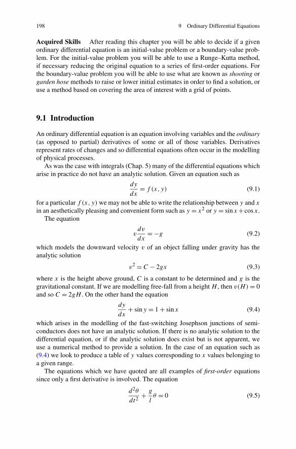
198 9 Ordinary Differential Equations
Acquired Skills After reading this chapter you will be able to decide if a givenordinary differential equation is an initial-value problem or a boundary-value prob-lem. For the initial-value problem you will be able to use a Runge–Kutta method,if necessary reducing the original equation to a series of first-order equations. Forthe boundary-value problem you will be able to use what are known as shooting orgarden hose methods to raise or lower initial estimates in order to find a solution, oruse a method based on covering the area of interest with a grid of points.
9.1 Introduction
An ordinary differential equation is an equation involving variables and the ordinary(as opposed to partial) derivatives of some or all of those variables. Derivativesrepresent rates of changes and so differential equations often occur in the modellingof physical processes.
As was the case with integrals (Chap. 5) many of the differential equations whicharise in practice do not have an analytic solution. Given an equation such as
dy
dx= f (x, y) (9.1)
for a particular f (x, y) we may not be able to write the relationship between y and x
in an aesthetically pleasing and convenient form such as y = x2 or y = sinx +cosx.The equation
vdv
dx= −g (9.2)
which models the downward velocity v of an object falling under gravity has theanalytic solution
v2 = C − 2gx (9.3)
where x is the height above ground, C is a constant to be determined and g is thegravitational constant. If we are modelling free-fall from a height H , then v(H) = 0and so C = 2gH . On the other hand the equation
dy
dx+ siny = 1 + sinx (9.4)
which arises in the modelling of the fast-switching Josephson junctions of semi-conductors does not have an analytic solution. If there is no analytic solution to thedifferential equation, or if the analytic solution does exist but is not apparent, weuse a numerical method to provide a solution. In the case of an equation such as(9.4) we look to produce a table of y values corresponding to x values belonging toa given range.
The equations which we have quoted are all examples of first-order equationssince only a first derivative is involved. The equation
d2θ
dt2+ g
lθ = 0 (9.5)
9.1 Introduction 199
which models the motion of a pendulum, is an example of a second-order equation.The order of a differential equation is defined by the order of the highest derivative.
In general, the solution to an nth-order differential equation contains n arbitraryconstants which may be determined by requiring the solution to satisfy n indepen-dent conditions particular to the application. We have already seen an example ofthis in the first-order equation (9.2) and its solution (9.3). If the solution is analyticthe arbitrary constants will be apparent, but even if an analytic solution does notexist, we are still required to provide sufficient independent conditions to determinethe solution uniquely.
As a further example consider the second-order equation (9.5) which has theanalytic solution
θ = A cosωt + B sinωt
where ω =√
gl
and A and B are constants to be determined. θ represents the angle
through which the pendulum swings, l is the length of the pendulum and t is themeasure of time. A and B may be uniquely determined by requiring the solutionto satisfy the two conditions θ(0) = θ0 and dθ
dt(0) = θ1, where θ0 and θ1 are known
values. These conditions model the release of the pendulum from angle θ0 withangular velocity θ1.
The problem of the falling body and the pendulum which we have just describedare examples of an initial-value problem. An initial-value problem is a differentialequation for which conditions relating to initial values of the independent variableare attached. As an initial-value problem (9.5) might be stated as
d2θ
dt2+ g
lθ = 0, θ(0) = θ0,
dθ
dt(0) = θ1.
The same equation (9.5) may be used to model the buckling of a rod. Using a dif-ferent notation we have
d2y
dx2+ Ky = 0 (9.6)
where x is measured along the rod, y is the lateral displacement and K is a con-stant related to the material properties of the rod. In this case the solution mightbe uniquely determined by requiring y(0) = 0 and y(L) = 0. These conditions areappropriate to a model of a beam of length L which is clamped at both ends. Wenow have what is known as a boundary-value problem. A boundary-value problemis a differential equation for which conditions relating to values of the independentvariable at more than one point are attached. As a boundary-value problem (9.6)might be stated as
d2y
dx2+ Ky = 0, y(0) = 0, y(L) = 0. (9.7)

200 9 Ordinary Differential Equations
9.2 First-Order Equations
We begin by studying methods for finding solutions of first-order equations. Suchequations are necessarily initial-value problems since only one condition, usuallyreferred to as an initial condition, is required for a unique solution. Our problem ingeneral terms may be stated as the initial-value problem
dy
dx= f (x, y), y(x0) = y0. (9.8)
9.2.1 Euler’s Method
Euler’s method is based on the approximation of dy/dx at x by (f (x + h) −f (x))/h, where h (the step-length) is some suitably small value. This formula,which we employed in Sect. 6.2, is used in (9.8) to compute y at x + h given y
at x and so from an initial starting point the solution may be advanced through agiven interval. The method is illustrated in the following problem.
Problem
Solve the following differential equation using Euler’s method.
dy
dx= 3x − y + 8, y(0) = 3.
Compute the solution from 0 to 0.5 using a step-length of 0.1. Compare this solutionwith the analytic solution, y = 3x − 2e−x + 5.
This initial-value problem is an example of a type which can occur in the mod-elling of changes in the population, y of a group of people, atomic particles, bacteriaor whatever over time, x. In this example we assume that the population increaseswith respect to time but that this increase is countered with a decrease proportionalto the size of the population. The rates of increase and decrease are 3x + 8 and −y
respectively.We assume that the model has been formed so that the solution measures the
population in appropriate multiples, and that overall the population is sufficientlylarge to allow the use of real numbers with a fractional part, rather than whole integernumbers.
Solution
Euler’s method advances the solution from x to x + h using the approximation
y(x + h) ≈ y(x) + hdy
dx
∣∣∣∣x
(9.9)
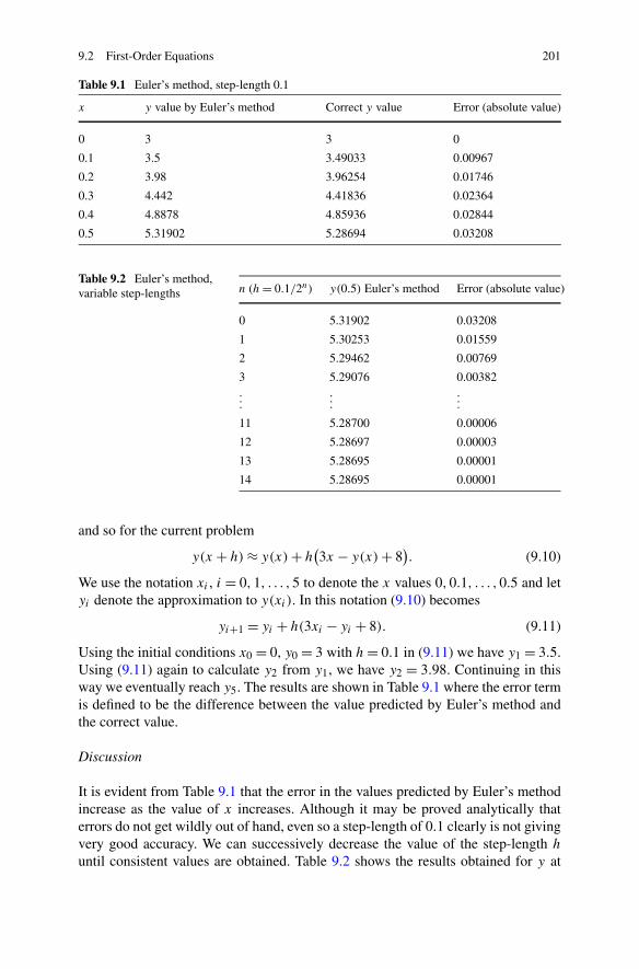
9.2 First-Order Equations 201
Table 9.1 Euler’s method, step-length 0.1
x y value by Euler’s method Correct y value Error (absolute value)
0 3 3 0
0.1 3.5 3.49033 0.00967
0.2 3.98 3.96254 0.01746
0.3 4.442 4.41836 0.02364
0.4 4.8878 4.85936 0.02844
0.5 5.31902 5.28694 0.03208
Table 9.2 Euler’s method,variable step-lengths n (h = 0.1/2n) y(0.5) Euler’s method Error (absolute value)
0 5.31902 0.03208
1 5.30253 0.01559
2 5.29462 0.00769
3 5.29076 0.00382...
.
.
....
11 5.28700 0.00006
12 5.28697 0.00003
13 5.28695 0.00001
14 5.28695 0.00001
and so for the current problem
y(x + h) ≈ y(x) + h(3x − y(x) + 8
). (9.10)
We use the notation xi , i = 0,1, . . . ,5 to denote the x values 0,0.1, . . . ,0.5 and letyi denote the approximation to y(xi). In this notation (9.10) becomes
yi+1 = yi + h(3xi − yi + 8). (9.11)
Using the initial conditions x0 = 0, y0 = 3 with h = 0.1 in (9.11) we have y1 = 3.5.Using (9.11) again to calculate y2 from y1, we have y2 = 3.98. Continuing in thisway we eventually reach y5. The results are shown in Table 9.1 where the error termis defined to be the difference between the value predicted by Euler’s method andthe correct value.
Discussion
It is evident from Table 9.1 that the error in the values predicted by Euler’s methodincrease as the value of x increases. Although it may be proved analytically thaterrors do not get wildly out of hand, even so a step-length of 0.1 clearly is not givingvery good accuracy. We can successively decrease the value of the step-length h
until consistent values are obtained. Table 9.2 shows the results obtained for y at
202 9 Ordinary Differential Equations
x = 0.5 by successively halving h. Having obtained agreement for two successivevalues of h we would normally stop the calculation at this point and assume wehave a valid result. It can be seen from the table that as h decreases linearly so doesthe error. This may be proved by analysis and so we may expect to obtain more andmore accuracy using a smaller and smaller step-length. However, decreasing thestep-length increases the number of arithmetic calculations and may mean that weare dealing with very small numbers, all of which is liable to increase the error inthe computation. Indeed our calculations, shown in the table above, could lead us toaccept a value of 5.28695 when the true value is 5.28694. In this case the differencemay not matter very much, but in practice could be significant.
Although Euler’s method may not be sufficiently accurate for some problems, theunderlying idea is a good one and can be used to good effect in forming the morepowerful Runge–Kutta methods.
9.2.2 Runge–Kutta Methods
Euler’s method for solving the initial-value problem (9.8) advances the solutionfrom x to x +h using the approximating formula (9.9). As an alternative we use thesame formula but with the derivative y′ evaluated at the mid-point of x and x +h. Itis envisaged that the derivative at the mid-point is more representative of the varyingderivative across the range. The approximating formula becomes
y(x + h) ≈ y(x) + hy′(
x + h
2
).
This approximation is the basis of the Runge–Kutta method, which is illustrated inthe following problem.
Problem
Solve the initial-value problem
dy
dx= 3x − y + 8, y(0) = 3
using the simple Runge–Kutta method. Compute the solution from 0 to 0.5 usinga step-length of 0.1. This is the same problem we used to illustrate Euler’s methodand is one to which we will return.
Solution
The method advances the solution from x to x + h using an increment given by
hy′(
x + h
2
)= hf
(x + h
2, y
(x + h
2
))where f (x, y) = 3x − y + 8.
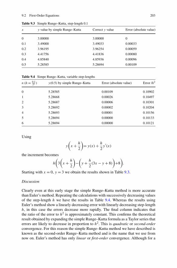
9.2 First-Order Equations 203
Table 9.3 Simple Runge–Kutta, step-length 0.1
x y value by simple Runge–Kutta Correct y value Error (absolute value)
0 3.00000 3.00000 0
0.1 3.49000 3.49033 0.00033
0.2 3.96195 3.96254 0.00059
0.3 4.41756 4.41836 0.00080
0.4 4.85840 4.85936 0.00096
0.5 5.28585 5.28694 0.00109
Table 9.4 Simpe Runge–Kutta, variable step-lengths
n (h = 0.12n ) y(0.5) by simple Runge–Kutta Error (absolute value) Error /h2
0 5.28585 0.00109 0.10902
1 5.28668 0.00026 0.10497
2 5.28687 0.00006 0.10301
3 5.28692 0.00002 0.10204
4 5.28693 0.00001 0.10156
5 5.28694 0.00000 0.10133
6 5.28694 0.00000 0.10121
Using
y
(x + h
2
)= y(x) + h
2y′(x)
the increment becomes
h
(3
(x + h
2
)−
(y + h
2(3x − y + 8)
)+8
).
Starting with x = 0, y = 3 we obtain the results shown in Table 9.3.
Discussion
Clearly even at this early stage the simple Runge–Kutta method is more accuratethan Euler’s method. Repeating the calculations with successively decreasing valuesof the step-length h we have the results in Table 9.4. Whereas the results usingEuler’s method show a linearly decreasing error with linearly decreasing step-lengthh, in this case the errors decrease more rapidly. The final column indicates thatthe ratio of the error to h2 is approximately constant. This confirms the theoreticalresult obtained by expanding the simple Runge–Kutta formula as a Taylor series thaterrors are likely to decrease in proportion to h2. This is quadratic or second-orderconvergence. For this reason the simple Runge–Kutta method we have described isknown as the second-order Runge–Kutta method and is the name that we use fromnow on. Euler’s method has only linear or first-order convergence. Although for a
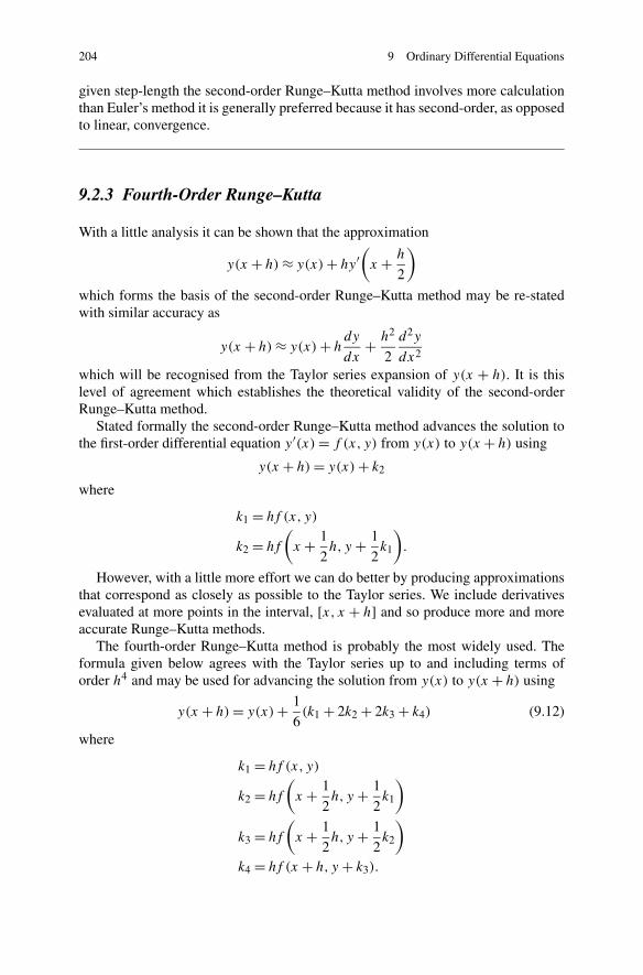
204 9 Ordinary Differential Equations
given step-length the second-order Runge–Kutta method involves more calculationthan Euler’s method it is generally preferred because it has second-order, as opposedto linear, convergence.
9.2.3 Fourth-Order Runge–Kutta
With a little analysis it can be shown that the approximation
y(x + h) ≈ y(x) + hy′(
x + h
2
)
which forms the basis of the second-order Runge–Kutta method may be re-statedwith similar accuracy as
y(x + h) ≈ y(x) + hdy
dx+ h2
2
d2y
dx2
which will be recognised from the Taylor series expansion of y(x + h). It is thislevel of agreement which establishes the theoretical validity of the second-orderRunge–Kutta method.
Stated formally the second-order Runge–Kutta method advances the solution tothe first-order differential equation y′(x) = f (x, y) from y(x) to y(x + h) using
y(x + h) = y(x) + k2
where
k1 = hf (x, y)
k2 = hf
(x + 1
2h,y + 1
2k1
).
However, with a little more effort we can do better by producing approximationsthat correspond as closely as possible to the Taylor series. We include derivativesevaluated at more points in the interval, [x, x + h] and so produce more and moreaccurate Runge–Kutta methods.
The fourth-order Runge–Kutta method is probably the most widely used. Theformula given below agrees with the Taylor series up to and including terms oforder h4 and may be used for advancing the solution from y(x) to y(x + h) using
y(x + h) = y(x) + 1
6(k1 + 2k2 + 2k3 + k4) (9.12)
where
k1 = hf (x, y)
k2 = hf
(x + 1
2h,y + 1
2k1
)
k3 = hf
(x + 1
2h,y + 1
2k2
)
k4 = hf (x + h,y + k3).
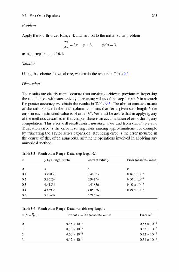
9.2 First-Order Equations 205
Problem
Apply the fourth-order Runge–Kutta method to the initial-value problem
dy
dx= 3x − y + 8, y(0) = 3
using a step-length of 0.1.
Solution
Using the scheme shown above, we obtain the results in Table 9.5.
Discussion
The results are clearly more accurate than anything achieved previously. Repeatingthe calculations with successively decreasing values of the step-length h in a searchfor greater accuracy we obtain the results in Table 9.6. The almost constant natureof the ratio shown in the final column confirms that for a given step-length h theerror in each estimated value is of order h4. We must be aware that in applying anyof the methods described in this chapter there is an accumulation of error during anycomputation. This error will result from truncation error and from rounding error.Truncation error is the error resulting from making approximations, for exampleby truncating the Taylor series expansion. Rounding error is the error incurred inthe course of the, often numerous, arithmetic operations involved in applying anynumerical method.
Table 9.5 Fourth-order Runge–Kutta, step-length 0.1
x y by Runge–Kutta Correct value y Error (absolute value)
0 3 3 0
0.1 3.49033 3.49033 0.16 × 10⁻⁶
0.2 3.96254 3.96254 0.30 × 10⁻⁶
0.3 4.41836 4.41836 0.40 × 10⁻⁶
0.4 4.85936 4.85936 0.49 × 10⁻⁶
0.5 5.28694 5.28694
Table 9.6 Fourth-order Runge–Kutta, variable step-lengths
n (h = 0.12n ) Error at x = 0.5 (absolute value) Error /h4
0 0.55 × 10⁻⁶ 0.55 × 10⁻²
1 0.33 × 10⁻⁷ 0.53 × 10⁻²
2 0.20 × 10⁻⁸ 0.52 × 10⁻²
3 0.12 × 10⁻⁹ 0.51 × 10⁻²
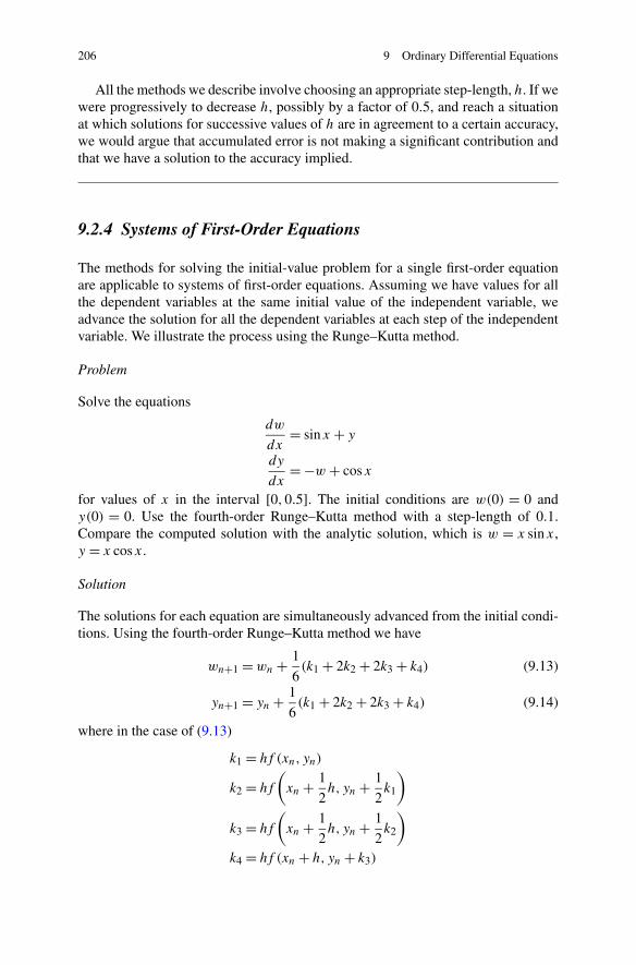
206 9 Ordinary Differential Equations
All the methods we describe involve choosing an appropriate step-length, h. If wewere progressively to decrease h, possibly by a factor of 0.5, and reach a situationat which solutions for successive values of h are in agreement to a certain accuracy,we would argue that accumulated error is not making a significant contribution andthat we have a solution to the accuracy implied.
9.2.4 Systems of First-Order Equations
The methods for solving the initial-value problem for a single first-order equationare applicable to systems of first-order equations. Assuming we have values for allthe dependent variables at the same initial value of the independent variable, weadvance the solution for all the dependent variables at each step of the independentvariable. We illustrate the process using the Runge–Kutta method.
Problem
Solve the equations
dw
dx= sinx + y
dy
dx= −w + cosx
for values of x in the interval [0,0.5]. The initial conditions are w(0) = 0 andy(0) = 0. Use the fourth-order Runge–Kutta method with a step-length of 0.1.Compare the computed solution with the analytic solution, which is w = x sinx,y = x cosx.
Solution
The solutions for each equation are simultaneously advanced from the initial condi-tions. Using the fourth-order Runge–Kutta method we have
wn+1 = wn + 1
6(k1 + 2k2 + 2k3 + k4) (9.13)
yn+1 = yn + 1
6(k1 + 2k2 + 2k3 + k4) (9.14)
where in the case of (9.13)
k1 = hf (xn, yn)
k2 = hf
(xn + 1
2h,yn + 1
2k1
)
k3 = hf
(xn + 1
2h,yn + 1
2k2
)
k4 = hf (xn + h,yn + k3)
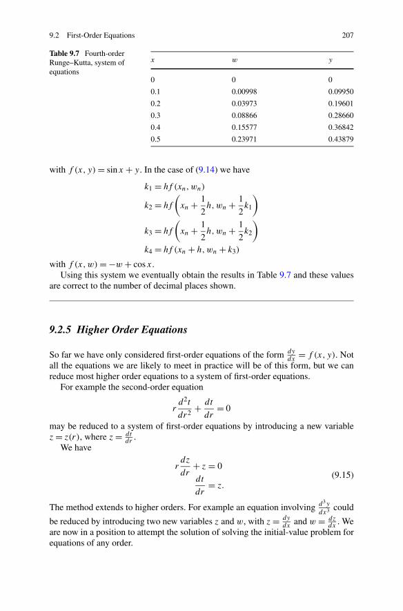
9.2 First-Order Equations 207
Table 9.7 Fourth-orderRunge–Kutta, system ofequations
x w y
0 0 0
0.1 0.00998 0.09950
0.2 0.03973 0.19601
0.3 0.08866 0.28660
0.4 0.15577 0.36842
0.5 0.23971 0.43879
with f (x, y) = sinx + y. In the case of (9.14) we have
k1 = hf (xn,wn)
k2 = hf
(xn + 1
2h,wn + 1
2k1
)
k3 = hf
(xn + 1
2h,wn + 1
2k2
)
k4 = hf (xn + h,wn + k3)
with f (x,w) = −w + cosx.Using this system we eventually obtain the results in Table 9.7 and these values
are correct to the number of decimal places shown.
9.2.5 Higher Order Equations
So far we have only considered first-order equations of the form dydx
= f (x, y). Notall the equations we are likely to meet in practice will be of this form, but we canreduce most higher order equations to a system of first-order equations.
For example the second-order equation
rd2t
dr2+ dt
dr= 0
may be reduced to a system of first-order equations by introducing a new variablez = z(r), where z = dt
dr.
We have
rdz
dr+ z = 0dt
dr= z.
(9.15)
The method extends to higher orders. For example an equation involving d3y
dx3 could
be reduced by introducing two new variables z and w, with z = dydx
and w = dzdx
. Weare now in a position to attempt the solution of solving the initial-value problem forequations of any order.
208 9 Ordinary Differential Equations
9.3 Boundary Value Problems
We consider problems for which the solution is required to meet specified condi-tions at both ends of a range. Two methods are presented, a method that for obviousreasons is known as the shooting or garden-hose method and a method which ap-proximates derivatives over the range using difference equations.
9.3.1 Shooting Method
Anyone who has used a garden hose, or has tried to hit any kind of target will knowthat there is a trial and error element involved. First attempts will either overshootthe target or fall short. However, this effort is not wasted since it usually gives anindication as to whether to raise or lower the aim. A similar scheme may be appliedto boundary-value problems. We form an initial-value problem, which we solve byone of the methods described earlier, by assuming a set of initial conditions and seewhere the solution leads. We then vary the initial conditions until we hit the targetat the other end. The following problem illustrates the method.
Problem
The following equation is an example of a type which arises in the modelling of thetemperature, y of a cooling fin at distance x from a base position.
d2y
dx2= 2y.
Find a solution using the shooting method which satisfies y = 1 at x = 0 anddy/dx = 0 at x = 1. Tabulate the solution at the points 0.1,0.2, . . . ,1. Comparethe result with analytic solution namely,
c1e√
2x + c2e−√
2x
where for this example, c1 = 0.05581 and c2 = 0.94419.
Solution
Writing z = dy/dx this second-order equation may be written as a system of first-order equations, namely
dz
dx= 2y
dy
dx= z
where y = y(x) and z = z(x) are such that y(0) = 1 and z(1) = 0.
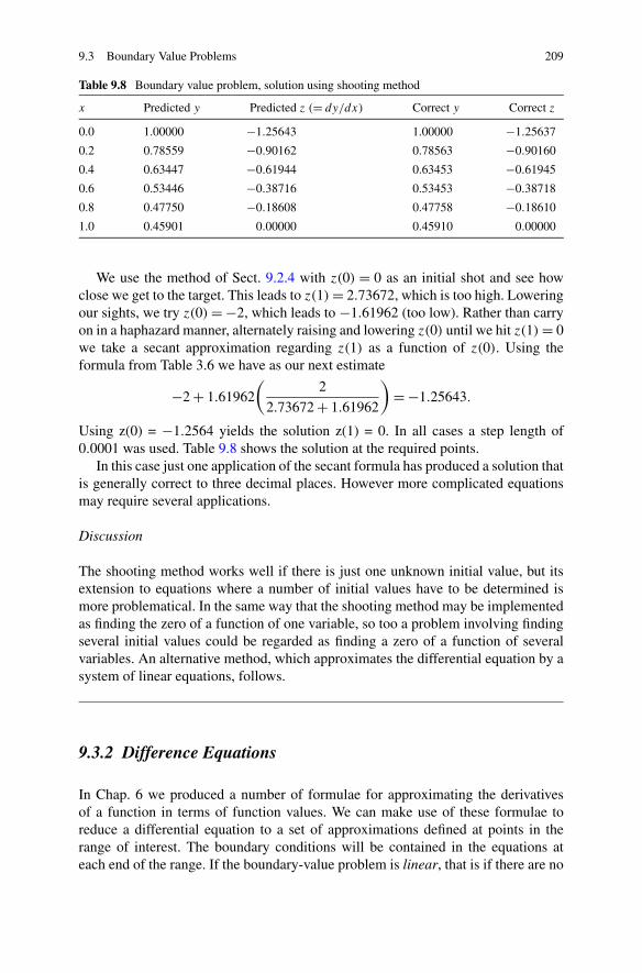
9.3 Boundary Value Problems 209
Table 9.8 Boundary value problem, solution using shooting method
x Predicted y Predicted z (= dy/dx) Correct y Correct z
0.0 1.00000 −1.25643 1.00000 −1.25637
0.2 0.78559 −0.90162 0.78563 −0.90160
0.4 0.63447 −0.61944 0.63453 −0.61945
0.6 0.53446 −0.38716 0.53453 −0.38718
0.8 0.47750 −0.18608 0.47758 −0.18610
1.0 0.45901 0.00000 0.45910 0.00000
We use the method of Sect. 9.2.4 with z(0) = 0 as an initial shot and see howclose we get to the target. This leads to z(1) = 2.73672, which is too high. Loweringour sights, we try z(0) = −2, which leads to −1.61962 (too low). Rather than carryon in a haphazard manner, alternately raising and lowering z(0) until we hit z(1) = 0we take a secant approximation regarding z(1) as a function of z(0). Using theformula from Table 3.6 we have as our next estimate
−2 + 1.61962
(2
2.73672 + 1.61962
)= −1.25643.
Using z(0) = −1.2564 yields the solution z(1) = 0. In all cases a step length of0.0001 was used. Table 9.8 shows the solution at the required points.
In this case just one application of the secant formula has produced a solution thatis generally correct to three decimal places. However more complicated equationsmay require several applications.
Discussion
The shooting method works well if there is just one unknown initial value, but itsextension to equations where a number of initial values have to be determined ismore problematical. In the same way that the shooting method may be implementedas finding the zero of a function of one variable, so too a problem involving findingseveral initial values could be regarded as finding a zero of a function of severalvariables. An alternative method, which approximates the differential equation by asystem of linear equations, follows.
9.3.2 Difference Equations
In Chap. 6 we produced a number of formulae for approximating the derivativesof a function in terms of function values. We can make use of these formulae toreduce a differential equation to a set of approximations defined at points in therange of interest. The boundary conditions will be contained in the equations ateach end of the range. If the boundary-value problem is linear, that is if there are no
210 9 Ordinary Differential Equations
terms involving products of derivatives, we have a system of linear equations. Wemay solve the linear system by Gaussian elimination and so solve the differentialequation in one fell swoop. By way of an example we use the previous cooling finproblem which is an example of a linear boundary-value problem.
Problem
Solve
d2y
dx2= 2y (9.16)
over the interval [0,1], where y(0) = 1 and dydx
(1) = 0, using difference equations.
Solution
Initially we take a step-length of 0.1 to divide the x interval [0,1] into 10 equalsub-intervals. Labelling the points xi, i = 0, . . . ,10 and using the approximation tothe second derivative, ((6.15), Chap. 6) we have
y′′(x) = y(x + h) − 2y(x) + y(x − h)
h2.
In this example y′′ = 2y, y0 = 1 and so
2yi = yi+1 − 2yi + yi−1
h2, i = 1, . . . ,9, y0 = 1.
The remaining equation of the ten we need to be able to find the 10 unknowns yi ,is supplied by substituting h = −0.1 and the boundary condition y′(1) = 0 in thetruncated Taylor series (6.2) to give
y9 = y10 + h2y10.
Putting h = 0.1 we have:
−2.02y1 + y2 = −1
y1 − 2.02y2 + y3 = 0
y2 − 2.02y3 + y4 = 0
. . .. . .
y8 − 2.02y9 + y10 = 0
y9 − 1.01y10 = 0.
A similar system, though one involving more equations may be constructed forshorter step-lengths. The results from solving such systems are shown in Table 9.9.
The results show that we are converging to a solution and this may be confirmedby comparing with the analytic solution given in the previous problem.
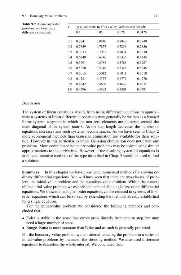
9.3 Boundary Value Problems 211
Table 9.9 Boundary valueproblem, solution usingdifference equations
x y(x) solutions to y′′(x) = 2y, various step-lengths
0.1 0.05 0.025 0.0125
0.1 0.8841 0.8840 0.8840 0.8840
0.2 0.7859 0.7857 0.7856 0.7856
0.3 0.7033 0.7031 0.7031 0.7030
0.4 0.6349 0.6346 0.6346 0.6345
0.5 0.5791 0.5788 0.5788 0.5787
0.6 0.5350 0.5346 0.5346 0.5345
0.7 0.5015 0.5012 0.5011 0.5010
0.8 0.4781 0.4777 0.4776 0.4776
0.9 0.4642 0.4638 0.4637 0.4637
1.0 0.4596 0.4592 0.4591 0.4591
Discussion
The system of linear equations arising from using difference equations to approxi-mate a systems of linear differential equations may generally be written as a bandedlinear system, a system in which the non-zero elements are clustered around themain diagonal of the system matrix. As the step-length decreases the number ofequations increases and such systems become sparse. As we have seen in Chap. 2more economical methods than Gaussian elimination are available for their solu-tion. However in this particular example Gaussian elimination does not cause anyproblems. More complicated boundary-value problems may be solved using similarapproximations to the derivatives. However, if the resulting system of equations isnonlinear, iterative methods of the type described in Chap. 3 would be used to finda solution.
Summary In this chapter we have considered numerical methods for solving or-dinary differential equations. You will have seen that there are two classes of prob-lem, the initial-value problem and the boundary-value problem. Within the contextof the initial-value problem we established methods for single first-order differentialequations. We showed that higher order equations can be reduced to systems of first-order equations which can be solved by extending the methods already establishedfor a single equation.
For the initial-value problem we considered the following methods and con-cluded that:
• Euler is stable in the sense that errors grow linearly from step to step, but mayneed a large number of steps.
• Runge–Kutta is more accurate than Euler and as such is generally preferred.
For the boundary-value problem we considered reducing the problem to a series ofinitial-value problems by means of the shooting method. We also used differenceequations to discretise the whole interval. We concluded that:
212 9 Ordinary Differential Equations
• Shooting methods work well if just one initial condition is unknown.• Difference equations are preferred if more than one initial condition is unknown.
Exercises
1. Write a Matlab program to implement Euler’s method to verify the results quotedin Sect. 9.2.1.
2. Write a Matlab function RK2 with heading
ynext = function RK2(f n, x, y,h)
to advance the solution to the first-order differential equation dy/dx = f n(x, y)
from a solution at (x, y) to a solution at (x = x + h) using the simple (second-order) Runge–Kutta method.
Assuming that the function f n(x, y) has been defined in a Matlab-M filef n.m the function would be called from a main program using a command suchas y2 = RK2(@fn, x1, y1,h).
Use the function to verify the results quoted in the chapter for
dy
dx= 3x − y + 8, y(0) = 3.
3. (i) Create a function RK4 with similar heading to RK2 to implement the fourth-order Runge–Kutta method. Test RK4 using the results quoted for the equationshown above.
(ii) Under certain conditions, taking into account gravity and air resistance,the speed v at time t of a projectile fired vertically into the air may be modelledby a first-order differential equation of the form
dv
dt= −9.81 − 0.2v2
by taking into account the force due to gravity and air resistance. If the pro-jectile is fired upwards with speed v = 10 show that the fourth-order Runge–Kutta method with a step length of 0.5 produces the results shown in Table 9.10.Though possible, extending the range much beyond t = 0.6 would not be mean-ingful since the projectile is about to reach zero velocity, at which point it fallsto earth and a different model applies. Repeat the calculation with step-length0.01 to suggest we have accuracy to 2 decimal places.
4. Use the function RK4 to solve the following simultaneous equations
dw
dx= sinx + y
dy
dx= −w + cosx
using the method described in Sect. 9.2.4. Advance the solutions for w and y
simultaneously using commands of the form
w = RK4(@fxy, x, y, h);y = RK4(@fwx, x , w, h);
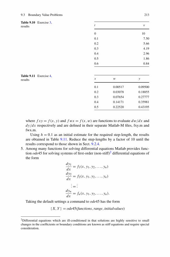
9.3 Boundary Value Problems 213
Table 9.10 Exercise 3,results t v
0 10
0.1 7.50
0.2 5.66
0.3 4.19
0.4 2.96
0.5 1.86
0.6 0.84
Table 9.11 Exercise 4,results x w y
0.1 0.00517 0.09500
0.2 0.03078 0.18855
0.3 0.07654 0.27777
0.4 0.14171 0.35981
0.5 0.22520 0.43195
where f xy = f (x, y) and f wx = f (x,w) are functions to evaluate dw/dx anddy/dx respectively and are defined in their separate Matlab-M files, fxy.m andfwx.m.
Using h = 0.1 as an initial estimate for the required step-length, the resultsare obtained in Table 9.11. Reduce the step-lengths by a factor of 10 until theresults correspond to those shown in Sect. 9.2.4.
5. Among many functions for solving differential equations Matlab provides func-tion ode45 for solving systems of first-order (non-stiff)2 differential equations ofthe form
dy1
dx= f1(x, y1, y2, . . . , yn)
dy2
dx= f2(x, y1, y2, . . . , yn)
... = ...dyn
dx= fn(x, y1, y2, . . . , yn).
Taking the default settings a command to ode45 has the form
[X,Y]= ode45(functions, range, initialvalues)
2Differential equations which are ill-conditioned in that solutions are highly sensitive to smallchanges in the coefficients or boundary conditions are known as stiff equations and require specialconsideration.

214 9 Ordinary Differential Equations
where range is a vector holding the range of points of the range of x values forwhich a solution is required (typically [ a b ]) or a set of specific points ([ a :increment : b]) and initialvalues is an n-element vector containing initial valuesy1, . . . , yn of the dependent variables. The parameter functions is the name ofthe function, which has two parameters x and y. For any value of x and a listof corresponding values y1, . . . , yn stored as elements of the n-element vector y
functions returns an n-element vector of derivatives dyi/dx.Use ode45 to solve the equations of question 4 and so verify the results quoted
in Sect. 9.2.4. Identifying x as the independent vector and w and y as dependentvectors a suitable command could be
[x,wyvec]= ode45(@sincos, [0 : 0.1 : 0.5], [0 0]);where sincos is the name of the M-file containing
function dy = sincos(x, y)dy = [ sin(x) + y(2); −y(1) + cos(x)];
The function returns w and y values (in that order) for corresponding x values inthe 2-column vector wyvec.
6. Verify the results shown for the problem discussed in Sect. 9.3.1 using either theMatlab provided function ode45 or your own RK4 with step-length 0.00001.
7. Write a Matlab program to verify the results quoted for the example of the useof difference equations quoted in Sect. 9.3.2. This will be mainly an exercise inmatrix manipulation. The program should be written to handle an arbitrary step-length h, which will determine the size of a coefficient matrix, A and a columnvector, b of right-sides. Use Matlab functions ones, diag, zeros and the back-slashoperator as shown in the program segment below, which would be appropriatefor building the coefficient matrix given n equations and step-length h.
% column vector of n 1’sv = ones(n, 1);
% row vector of n−1 1’sw = ones(1, n−1);
% place −2 + h∧2 on the main diagonal% place 1’s on the diagonals above and below the main diagonal
A = diag(w, −1) + diag( −2∗(1+h∧2)∗v, 0) + diag(w, 1);% build the right hand side column vector
b = zeros(n, 1);% modify A and b to allow for the boundary conditions
A(n, n) = −(1+h∧2);b(1) = −1;
% solve the equationsx = A\b;
Chapter 10Eigenvalues and Eigenvectors
Aims In this chapter we investigate methods for determining some, or all, of theeigenvalues and eigenvectors1 of a square matrix A.
Overview It is convenient to divide methods for determining eigenvalues andeigenvectors into those which either
• locate a single eigenvalue/eigenvector pair
or
• determine all eigenvalues and eigenvectors.
We show how eigenvalues may be found using the characteristic polynomial andhow the power method locates a single eigenvalue/eigenvector pair. We also showhow eigenvalues can be found by transforming a general matrix into upper triangularform. Having shown how an eigenvector corresponding to a given eigenvalue maybe found we are in a position to find all the eigenvalues and eigenvectors of a matrix.
Acquired Skills After reading this chapter you will
• understand the significance of eigenvalues and eigenvectors.• know how to use methods for locating a single eigenvalue/eigenvector pair.• know how to use a method for locating all eigenvalue/eigenvector pairs.• have an appreciation of what is known in the literature as The Eigenvalue problem.
10.1 Introduction
Eigenvalues and eigenvectors occur in the study of differential equations which areused in modelling vibrational problems in science and engineering. Examples of
1The word eigen translates from the German as own, intrinsic or inherent.
C. Woodford, C. Phillips, Numerical Methods with Worked Examples: Matlab Edition,DOI 10.1007/978-94-007-1366-6_10, © Springer Science+Business Media B.V. 2012
215
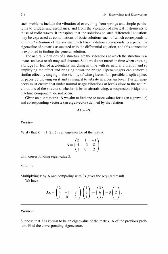
216 10 Eigenvalues and Eigenvectors
such problems include the vibration of everything from springs and simple pendu-lums to bridges and aeroplanes, and from the vibration of musical instruments tothose of radio waves. It transpires that the solutions to such differential equationsmay be expressed as combinations of basic solutions each of which corresponds toa natural vibration of the system. Each basic solution corresponds to a particulareigenvalue of a matrix associated with the differential equation, and this connectionis exploited in finding the general solution.
The natural vibrations of a structure are the vibrations at which the structure res-onates and as a result may self destruct. Soldiers do not march in time when crossinga bridge for fear of accidentally marching in time with its natural vibration and soamplifying the effect and bringing down the bridge. Opera singers can achieve asimilar effect by singing in the vicinity of wine glasses. It is possible to split a pieceof paper by blowing on it and causing it to vibrate at a certain level. Design engi-neers must ensure that under normal usage vibrations at levels close to the naturalvibrations of the structure, whether it be an aircraft wing, a suspension bridge or amachine component, do not occur.
Given an n×n matrix, A we aim to find one or more values for λ (an eigenvalue)and corresponding vector x (an eigenvector) defined by the relation
Ax = λx.
Problem
Verify that x = (1,2,1) is an eigenvector of the matrix
A =⎛⎝
2 1 −14 −3 81 0 2
⎞⎠
with corresponding eigenvalue 3.
Solution
Multiplying x by A and comparing with 3x gives the required result.We have
Ax =⎛⎝
2 1 −14 −3 81 0 2
⎞⎠
⎛⎝
121
⎞⎠ =
⎛⎝
363
⎞⎠ = 3
⎛⎝
121
⎞⎠ .
Problem
Suppose that 3 is known to be an eigenvalue of the matrix, A of the previous prob-lem. Find the corresponding eigenvector.
10.2 The Characteristic Polynomial 217
Solution
We solve the system of equations Ax = 3x. Letting x = (x1, x2, x3) we have
2x1 + x2 − x3 = 3x1
4x1 − 3x2 + 8x3 = 3x2
x1 + 2x3 = 3x3
and so
−x1 + x2 − x3 = 0
4x1 − 6x2 + 8x3 = 0
x1 − x3 = 0.
Gaussian elimination produces the upper triangular system
−x1 + x2 − x3 = 0
−2x2 + 4x3 = 0
0x3 = 0.
Thus there is no unique solution and so we are free to set one of the variablesto whatever we choose. Letting x3 = 1, we have x2 = 2 and x1 = 1 from back-substitution.
Discussion
We have shown in this example that eigenvectors are not unique. By setting x3to any constant we can show that any multiple of (1,2,1) is an eigenvector of Acorresponding to the eigenvalue 3.
For any vector v the normalised form is defined to be v/norm(v) and so thenorm of a normalised vector is 1. Being able to assume that vectors (and in particulareigenvectors) are presented in normalised form can sometimes simplify subsequentdiscussion.
10.2 The Characteristic Polynomial
We may write Ax = λx in the form
(A − λI)x = 0
where, as before, x is the eigenvector corresponding to an eigenvalue λ of the matrixA of order n and I is the identity matrix of order n. The determinant of the matrixA − λI is a polynomial in λ and is known as the characteristic polynomial. Thecharacteristic polynomial provides a means of identifying eigenvalues.
218 10 Eigenvalues and Eigenvectors
Problem
Use the characteristic polynomial to find the eigenvalues of the matrix
A =(
4 1−5 −2
).
Solution
The characteristic polynomial, p(λ) is given by the determinant of the matrix(
4 − λ 1−5 −2 − λ
).
Therefore
p(λ) = (4 − λ)(−2 − λ) + 5
= λ2 − 2λ − 3
= (λ − 3)(λ + 1).
Since the system of equations, Ax = λx does not have a unique solution, the coeffi-cient matrix, A is singular, and so columns (and rows) are linearly dependent whichis equivalent to the determinant being zero. Setting p(λ) = 0 we have eigenvalues,λ = 3 and λ = −1.
Discussion
In principle we have shown a method for locating eigenvalues, although the costof forming p and then using an appropriate root-finding technique from Chap. 3might be prohibitively time consuming for large matrices. The characteristic poly-nomial can be used to determine all the eigenvalues but information as to eigenvec-tors would have to be found by solving the appropriate linear system. Note that thecharacteristic polynomial indicates that an n × n matrix has n eigenvalues and so itis possible that some eigenvalues may be identical and some may occur as complexconjugate pairs.
10.3 The Power Method
We present a method that can be used to find the largest eigenvalue of a matrix andthe corresponding eigenvector. Essentially the same method may be applied to findthe smallest eigenvalue and corresponding eigenvector. The method is explainedusing the example below. We use the terms largest and smallest to mean largest andsmallest in absolute value.
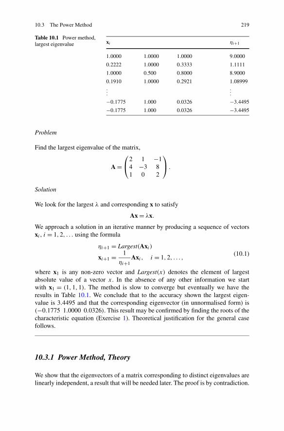
10.3 The Power Method 219
Table 10.1 Power method,largest eigenvalue xi ηi+1
1.0000 1.0000 1.0000 9.0000
0.2222 1.0000 0.3333 1.1111
1.0000 0.500 0.8000 8.9000
0.1910 1.0000 0.2921 1.08999...
.
.
.
−0.1775 1.000 0.0326 −3.4495
−0.1775 1.000 0.0326 −3.4495
Problem
Find the largest eigenvalue of the matrix,
A =⎛⎝
2 1 −14 −3 81 0 2
⎞⎠ .
Solution
We look for the largest λ and corresponding x to satisfy
Ax = λx.
We approach a solution in an iterative manner by producing a sequence of vectorsxi , i = 1,2, . . . using the formula
ηi+1 = Largest(Axi )
xi+1 = 1
ηi+1Axi , i = 1,2, . . . ,
(10.1)
where x1 is any non-zero vector and Largest(x) denotes the element of largestabsolute value of a vector x. In the absence of any other information we startwith x1 = (1,1,1). The method is slow to converge but eventually we have theresults in Table 10.1. We conclude that to the accuracy shown the largest eigen-value is 3.4495 and that the corresponding eigenvector (in unnormalised form) is(−0.1775 1.0000 0.0326). This result may be confirmed by finding the roots of thecharacteristic equation (Exercise 1). Theoretical justification for the general casefollows.
10.3.1 Power Method, Theory
We show that the eigenvectors of a matrix corresponding to distinct eigenvalues arelinearly independent, a result that will be needed later. The proof is by contradiction.
220 10 Eigenvalues and Eigenvectors
We assume the eigenvectors of the matrix are linearly dependent and show that thisleads to a contradiction.
Suppose that the n × n matrix A has distinct eigenvalues λ1, λ2, . . . , λm withcorresponding eigenvectors x1,x2, . . . ,xm. We know from the degree of the charac-teristic polynomial that m must be ≤ n. If xk is the first of the eigenvectors to be alinear combination of the eigenvectors x1,x2, . . . ,xk−1 we have
xk =k−1∑i=1
αixi (10.2)
where not all the αi are zero. By pre-multiplying both sides of (10.2) by A we findthat this implies
Axk =k−1∑i=1
αi(λk − λi)xi = 0. (10.3)
Since the terms λk − λi in the above are not all zero (10.3) shows that xk isnot the first of the eigenvectors to be a linear combination of the eigenvectorsx1,x2, . . . ,xk−1. This contradiction provides the required result, which we use toestablish the validity of (10.1).
We assume that we have an n × n matrix A with distinct n eigenvalues, which aswe have seen will have corresponding eigenvectors ξi , i = 1, . . . , n that are linearlyindependent. We also assume that the eigenvectors and eigenvalues λi are orderedso that
|λ1| > |λ2| ≥ |λ3| ≥ · · · ≥ |λn|.Since the eigenvectors of A are linearly independent for any vector x of the samedimension we have
x =n∑
i=1
αiξi
where the αi are constants and the ξi are the eigenvectors of A with correspondingeigenvalues λi . We make the further assumptions that α1 �= 0 and that the eigen-values are real (not complex). It may appear that we are making a number of as-sumptions but the procedure may be modified to deal with more general situations.It follows that
Ax =n∑
i=1
Aαiξi =n∑
i=1
αiλiξi
and so
Akx =n∑
i=1
αiλki ξi = λk
1
n∑i=1
αi
(λi
λ1
)k
ξi .
Going to the limit and noting that ξ1 is the eigenvalue of largest absolute value
limk→∞ Akx = lim
k→∞α1λk1ξ1
10.3 The Power Method 221
and so taking largest values
limk→∞
Largest(Ak+1x)
Largest(Akx)= lim
k→∞λk+1
1
λk1
= λ1.
We can connect this results with the sequence (10.1), which generates a sequence ηi
η3 = Largest(A2x1)
Largest(Ax1), η4 = Largest(A3x1)
Largest(A2x1), . . . , ηk+1 = Largest(Akx1)
Largest(Ak−1x1)
and confirms that η → λ1, whatever the value of x1.We may use the same technique to find the smallest eigenvalue of a matrix. For
any eigenvalue λ and corresponding eigenvector x of a matrix A we have
Ax = λx and so1
λx = A−1x.
In particular, if λ is the smallest eigenvalue of A, then it is the largest eigenvalueof the inverse, A−1. The corresponding eigenvector is the same in each case. If weapply the power method to finding the largest eigenvalue of A−1 we would approacha solution in an iterative manner by producing a sequence of vectors xi , i = 1,2, . . .
using the formula
A−1xi = λixi+1, i = 1,2, . . . . (10.4)
However, rather than calculate A−1 directly, we use the following form.
λiAxi+1 = xi , i = 1,2, . . . . (10.5)
Starting with an arbitrary x1 at each step we would solve the linear system
Axi+1 = 1
λi
xi , i = 1,2, . . .
where λi is the element of largest absolute value of the vector xi . The method isillustrated in the following problem.
Problem
Find the smallest eigenvalue of the matrix A given by
A =⎛⎝
2 1 −14 −3 81 0 2
⎞⎠ .
Solution
Starting with x1 = (1,1,1) and setting λi to the value of the maximum elementof xi , we solve the linear system (10.5) at each step to find xi+1 to give the re-sults shown in Table 10.2. However if the linear system is solved at the first step
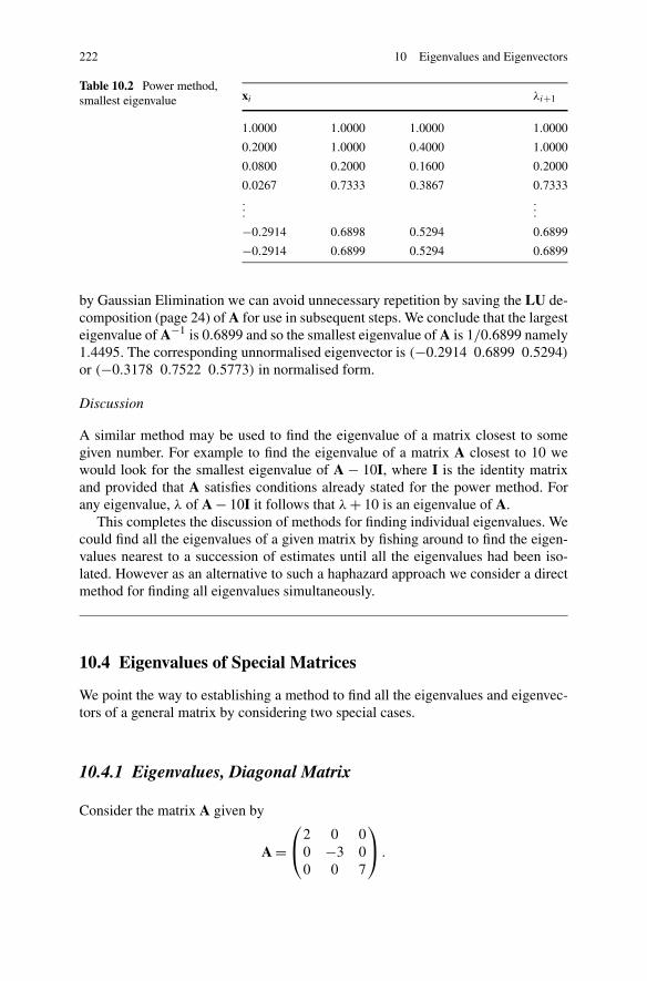
222 10 Eigenvalues and Eigenvectors
Table 10.2 Power method,smallest eigenvalue xi λi+1
1.0000 1.0000 1.0000 1.0000
0.2000 1.0000 0.4000 1.0000
0.0800 0.2000 0.1600 0.2000
0.0267 0.7333 0.3867 0.7333...
.
.
.
−0.2914 0.6898 0.5294 0.6899
−0.2914 0.6899 0.5294 0.6899
by Gaussian Elimination we can avoid unnecessary repetition by saving the LU de-composition (page 24) of A for use in subsequent steps. We conclude that the largesteigenvalue of A−1 is 0.6899 and so the smallest eigenvalue of A is 1/0.6899 namely1.4495. The corresponding unnormalised eigenvector is (−0.2914 0.6899 0.5294)
or (−0.3178 0.7522 0.5773) in normalised form.
Discussion
A similar method may be used to find the eigenvalue of a matrix closest to somegiven number. For example to find the eigenvalue of a matrix A closest to 10 wewould look for the smallest eigenvalue of A − 10I, where I is the identity matrixand provided that A satisfies conditions already stated for the power method. Forany eigenvalue, λ of A − 10I it follows that λ + 10 is an eigenvalue of A.
This completes the discussion of methods for finding individual eigenvalues. Wecould find all the eigenvalues of a given matrix by fishing around to find the eigen-values nearest to a succession of estimates until all the eigenvalues had been iso-lated. However as an alternative to such a haphazard approach we consider a directmethod for finding all eigenvalues simultaneously.
10.4 Eigenvalues of Special Matrices
We point the way to establishing a method to find all the eigenvalues and eigenvec-tors of a general matrix by considering two special cases.
10.4.1 Eigenvalues, Diagonal Matrix
Consider the matrix A given by
A =⎛⎝
2 0 00 −3 00 0 7
⎞⎠ .
10.5 A Simple QR Method 223
The characteristic polynomial, p(λ) for A is given by
p(λ) = (λ − 2)(λ + 3)(λ − 7).
The roots of p(λ) are clearly 2, −3 and 7 and so we have the eigenvalues. Thecorresponding eigenvectors are (1,0,0), (0,1,0) and (0,0,1).
The result generalises. The eigenvalues of an n × n diagonal matrix are the di-agonal elements. The corresponding eigenvectors are the columns of the identitymatrix of order n namely, (1,0, . . . ,0), (0,1,0, . . . ,0), . . . , (0,0, . . . ,0,1).
10.4.2 Eigenvalues, Upper Triangular Matrix
Consider the matrix A given by
A =⎛⎝
2 2 10 −3 40 0 7
⎞⎠ .
The characteristic polynomial, p(λ) for A is given by the determinant
p(λ) =∣∣∣∣∣∣2 − λ 2 1
0 −3 − λ 40 0 7 − λ
∣∣∣∣∣∣
and so the eigenvalues are the diagonal elements, 2, −3 and 7, as for a diagonalmatrix. The result generalises to upper triangular matrices of any order.
10.5 A Simple QR Method
Since we have a method for finding the eigenvalues (and hence the eigenvectors)of upper triangular matrices, we aim to transform more general matrices into thisform in such a way that we do not lose track of the original eigenvalues. If λ is aneigenvalue of A with corresponding eigenvector x we have for any matrix R
RAx = λRx. (10.6)
Furthermore(RAR−1)Rx = λRx
and so RAR−1 has the same eigenvalues as A but with corresponding eigenvectorsRx, where x is an eigenvector of A. Such a transformation of A to RAR−1 is knownas a similarity transformation. If we can make a similarity transformation of A toupper triangular form, the eigenvalues of the upper triangular matrix, namely thevalues of the diagonal elements, will be the eigenvalues of A. The eigenvectors ofA can be recovered from those of RAR−1.
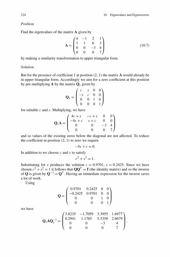
224 10 Eigenvalues and Eigenvectors
Problem
Find the eigenvalues of the matrix A given by
A =
⎛⎜⎜⎝
4 −1 2 11 1 6 30 0 −3 40 0 0 7
⎞⎟⎟⎠ (10.7)
by making a similarity transformation to upper triangular form.
Solution
But for the presence of coefficient 1 at position (2,1) the matrix A would already bein upper triangular form. Accordingly we aim for a zero coefficient at this positionby pre-multiplying A by the matrix Q1 given by
Q1 =
⎛⎜⎜⎝
c s 0 0−s c 0 00 0 1 00 0 0 1
⎞⎟⎟⎠
for suitable c and s. Multiplying, we have
Q1A =
⎛⎜⎜⎝
4c + s −c + s 0 0−4s + c s + c 0 0
0 0 −3 40 0 0 7
⎞⎟⎟⎠
and so values of the existing zeros below the diagonal are not affected. To reducethe coefficient in position (2,1) to zero we require
−4s + c = 0.
In addition to we choose c and s to satisfy
c2 + s2 = 1.
Substituting for s produces the solution c = 0.9701, s = 0.2425. Since we havechosen c2 + s2 = 1 it follows that QQT = I (the identity matrix) and so the inverseof Q is given by Q−1 = QT . Having an immediate expression for the inverse savesa lot of work.
Using
Q =
⎛⎜⎜⎝
0.9701 0.2425 0 0−0.2425 0.9701 0 0
0 0 1 00 0 0 1
⎞⎟⎟⎠
we have
Q1AQ−11 =
⎛⎜⎜⎝
3.8235 −1.7059 3.3955 1.69770.2941 1.1765 5.3358 2.6679
0 0 −3 40 0 0 7
⎞⎟⎟⎠ .
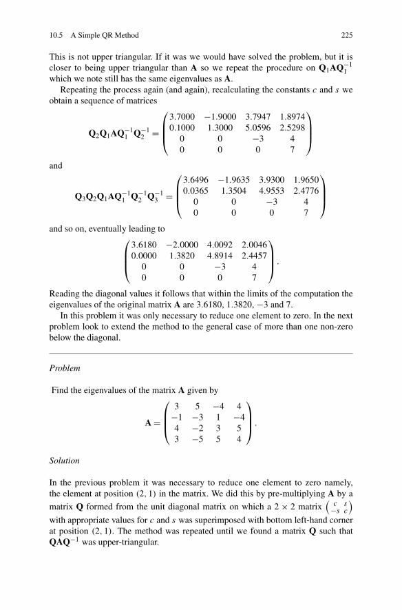
10.5 A Simple QR Method 225
This is not upper triangular. If it was we would have solved the problem, but it iscloser to being upper triangular than A so we repeat the procedure on Q1AQ−1
1which we note still has the same eigenvalues as A.
Repeating the process again (and again), recalculating the constants c and s weobtain a sequence of matrices
Q2Q1AQ−11 Q−1
2 =
⎛⎜⎜⎝
3.7000 −1.9000 3.7947 1.89740.1000 1.3000 5.0596 2.5298
0 0 −3 40 0 0 7
⎞⎟⎟⎠
and
Q3Q2Q1AQ−11 Q−1
2 Q−13 =
⎛⎜⎜⎝
3.6496 −1.9635 3.9300 1.96500.0365 1.3504 4.9553 2.4776
0 0 −3 40 0 0 7
⎞⎟⎟⎠
and so on, eventually leading to⎛⎜⎜⎝
3.6180 −2.0000 4.0092 2.00460.0000 1.3820 4.8914 2.4457
0 0 −3 40 0 0 7
⎞⎟⎟⎠ .
Reading the diagonal values it follows that within the limits of the computation theeigenvalues of the original matrix A are 3.6180, 1.3820, −3 and 7.
In this problem it was only necessary to reduce one element to zero. In the nextproblem look to extend the method to the general case of more than one non-zerobelow the diagonal.
Problem
Find the eigenvalues of the matrix A given by
A =
⎛⎜⎜⎝
3 5 −4 4−1 −3 1 −44 −2 3 53 −5 5 4
⎞⎟⎟⎠ .
Solution
In the previous problem it was necessary to reduce one element to zero namely,the element at position (2,1) in the matrix. We did this by pre-multiplying A by a
matrix Q formed from the unit diagonal matrix on which a 2 × 2 matrix(
c s−s c
)
with appropriate values for c and s was superimposed with bottom left-hand cornerat position (2,1). The method was repeated until we found a matrix Q such thatQAQ−1 was upper-triangular.
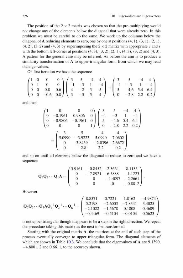
226 10 Eigenvalues and Eigenvectors
The position of the 2 × 2 matrix was chosen so that the pre-multiplying wouldnot change any of the elements below the diagonal that were already zero. In thisproblem we must be careful to do the same. We work up the columns below thediagonal of A reducing elements to zero, one by one at positions (4,1), (3,1), (2,1),(4,2), (3,2) and (4,3) by superimposing the 2 × 2 matrix with appropriate c and s
with the bottom left-corner at positions (4,3), (3,2), (2,1), (4,3), (3,2) and (4,3).A pattern for the general case may be inferred. As before the aim is to produce asimilarity transformation of A to upper-triangular form, from which we may readthe eigenvalues.
On first iteration we have the sequence⎛⎜⎜⎝
1 0 0 00 1 0 00 0 0.8 0.60 0 −0.6 0.8
⎞⎟⎟⎠
⎛⎜⎜⎝
3 5 −4 4−1 −3 1 −44 −2 3 53 −5 5 4
⎞⎟⎟⎠ =
⎛⎜⎜⎝
3 5 −4 4−1 −3 1 −45 −4.6 5.4 6.40 −2.8 2.2 0.2
⎞⎟⎟⎠
and then⎛⎜⎜⎝
1 0 0 00 −0.1961 0.9806 00 −0.9806 −0.1961 00 0 0 1
⎞⎟⎟⎠
⎛⎜⎜⎝
3 5 −4 4−1 −3 1 −45 −4.6 5.4 6.40 −2.8 2.2 0.2
⎞⎟⎟⎠
=
⎛⎜⎜⎝
3 5 −4 45.0990 −3.9223 5.0990 7.0602
0 3.8439 −2.0396 2.66720 −2.8 2.2 0.2
⎞⎟⎟⎠
and so on until all elements below the diagonal to reduce to zero and we have asequence
Q6Q5 · · ·Q1A =
⎛⎜⎜⎝
5.9161 −0.8452 2.3664 8.11350 −7.8921 6.5888 −1.12230 0 −1.4097 −2.26610 0 0 −0.8812
⎞⎟⎟⎠ .
However
Q6Q5 · · ·Q1AQ−11 Q−1
2 · · ·Q−16 =
⎛⎜⎜⎝
8.8571 0.7221 1.8162 −4.98745.2198 −2.6003 −7.8341 3.4025
−2.1022 −1.5678 0.1808 0.4609−0.4469 −0.5104 −0.0103 0.5623
⎞⎟⎟⎠
is not upper triangular though it appears to be a step in the right direction. We repeatthe procedure taking this matrix as the next to be transformed.
Starting with the original matrix A, the matrices at the end of each step of theprocess eventually converge to upper triangular form. The diagonal elements ofwhich are shown in Table 10.3. We conclude that the eigenvalues of A are 9.1390,−4.8001, 2 and 0.6611, to the accuracy shown.

10.5 A Simple QR Method 227
Table 10.3 Eigenvalues,simple QR method Diagonal elements
8.8571 −2.6003 0.1808 0.5623
9.2761 −5.0723 2.3788 0.4174
9.3774 −4.7131 1.7347 0.6011
9.0837 −4.8242 2.1016 0.6388
9.1839 −4.7996 1.9616 0.6541
9.1188 −4.7962 2.0187 0.6587
9.1504 −4.8041 1.9934 0.6603...
.
.
.
9.1391 −4.8002 2.0000 0.6611
9.1390 −4.8001 2.0000 0.6611
9.1390 −4.8001 2.0000 0.6611
Table 10.4 Simple QR method
Step 1 Find a matrix Q such that QA is upper triangular
Step 2 If QAQ−1 is upper triangular then stop. The elements of the diagonal are the eigenvalues
Step 3 Repeat from step 1
Discussion
The method we have described for finding the eigenvalues of a general matrix maybe formalised as shown in Table 10.4. The QR method was invented by Francis2 in1961 who used the terms Q and R, hence the name. The version we have describedis a simplified version, which though theoretically sound can be slow to convergeand may be defeated by rounding error. Problems involving matrices having equalor complex eigenvalues have not been considered. Over time a great deal of workhas been done to improve QR, which is one of the most widely used and importantmethods of numerical computation.
Summary In this chapter we have considered the practical importance of TheEigenvalue problem in science and engineering. We have shown the need for calcu-lating eigenvalues, which may be achieved in a number of ways. For finding singleeigenvalues we described the characteristic polynomial and the power method. Hav-ing found an eigenvalue we showed how the corresponding eigenvector could befound by solving a linear system. We showed how eigenvectors may be expressedin normalised form.
2John G.F. Francis, English computer scientist (1934–). Working independently Russian mathe-matician Vera Kublanovskaya also proposed the method in the same year.
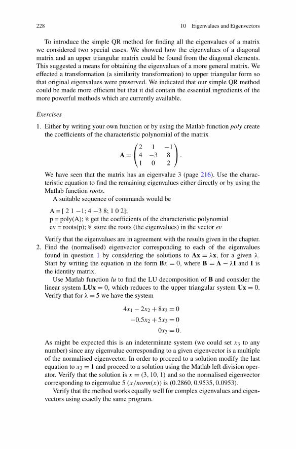
228 10 Eigenvalues and Eigenvectors
To introduce the simple QR method for finding all the eigenvalues of a matrixwe considered two special cases. We showed how the eigenvalues of a diagonalmatrix and an upper triangular matrix could be found from the diagonal elements.This suggested a means for obtaining the eigenvalues of a more general matrix. Weeffected a transformation (a similarity transformation) to upper triangular form sothat original eigenvalues were preserved. We indicated that our simple QR methodcould be made more efficient but that it did contain the essential ingredients of themore powerful methods which are currently available.
Exercises
1. Either by writing your own function or by using the Matlab function poly createthe coefficients of the characteristic polynomial of the matrix
A =⎛⎝
2 1 −14 −3 81 0 2
⎞⎠ .
We have seen that the matrix has an eigenvalue 3 (page 216). Use the charac-teristic equation to find the remaining eigenvalues either directly or by using theMatlab function roots.
A suitable sequence of commands would be
A = [ 2 1 −1; 4 −3 8; 1 0 2];p = poly(A); % get the coefficients of the characteristic polynomialev = roots(p); % store the roots (the eigenvalues) in the vector ev
Verify that the eigenvalues are in agreement with the results given in the chapter.2. Find the (normalised) eigenvector corresponding to each of the eigenvalues
found in question 1 by considering the solutions to Ax = λx, for a given λ.Start by writing the equation in the form Bx = 0, where B = A − λI and I isthe identity matrix.
Use Matlab function lu to find the LU decomposition of B and consider thelinear system LUx = 0, which reduces to the upper triangular system Ux = 0.Verify that for λ = 5 we have the system
4x1 − 2x2 + 8x3 = 0
−0.5x2 + 5x3 = 0
0x3 = 0.
As might be expected this is an indeterminate system (we could set x3 to anynumber) since any eigenvalue corresponding to a given eigenvector is a multipleof the normalised eigenvector. In order to proceed to a solution modify the lastequation to x3 = 1 and proceed to a solution using the Matlab left division oper-ator. Verify that the solution is x = (3,10,1) and so the normalised eigenvectorcorresponding to eigenvalue 5 (x/norm(x)) is (0.2860,0.9535,0.0953).
Verify that the method works equally well for complex eigenvalues and eigen-vectors using exactly the same program.
10.5 A Simple QR Method 229
Answers may also be verified using the Matlab supplied function eig for find-ing eigenvalues and eigenvectors. For a given matrix A, the command [v, e] =eig(A) would produce a matrix, v whose columns are eigenvectors of A and adiagonal matrix, e of corresponding eigenvalues.
3. Write a program to implement the power method. Make two versions, one forthe largest eigenvalue and another for the smallest (in absolute values). Use theprograms to verify the results shown in Sect. 10.3. In addition use one of theprograms to find the eigenvalue of
A =⎛⎝
2 1 −14 −3 81 0 2
⎞⎠
closest to −0.5.4. (i) Write a program to apply the simple QR method to the first problem of
Sect. 10.5. Build the sequence Q1AQ−11 ,Q2Q1AQ−1
1 Q−12 , . . . with each iter-
ation until the absolute value of element (2,1) of the matrix QAQ−1 whereQ = Qn · · ·Q2Q1, for some n is less than 1.0e-6.
Having completed the code for Step 1 of the QR method, Step 2 follows bywrapping Step 1 in a while loop. Assuming A has been established the programmight take the following form
while abs(A(2, 1)) > 1.0e-6;% solve -A(1, 1)∗s + A(2, 1)∗c = 0; s∧ 2 + c∧2 = 1;s = 1/sqrt(1 + (A(1, 1)/A(2, 1))∧2);c = s ∗( A(1, 1)/A(2, 1));Q = [ c s 0 0; −s c 0 0; 0 0 1 0; 0 0 0 1];A = Q∗A∗Q'; % inverse Q = Q'
end;
(ii) Find the normalised eigenvectors corresponding to the eigenvalues found inpart(i) using the method of question 1.
Note that Matlab supplies a function qr to provide the QR factorisation of amatrix. For example a command of the form [Q R] = qr(A); would for a givenmatrix A return a unitary Q (a matrix such that Q−1 = QT ) and upper triangularmatrix R such that QR = A. However when applied to the examples quoted in thechapter the function takes a slightly different route in that the signs of variablesc and s (using the notation of the chapter) are reversed, in solving for c and s thenegative square root is chosen.
5. Extend the program of question 4(i) to apply the QR method to the second prob-lem of Sect. 10.5. You might find it easier to repeat similar code from the previousquestion, cutting and pasting with a little editing to make separate code for eachof the six elements to be reduced to zero. Having spotted the pattern you mightthen try to shorten the program by using suitable loops to calculate c and s (usingthe notation of the main text) and position the c and s sub-matrix automatically.Use the norm of the vector of diagonal elements of QAQ−1 at the end of step 1as the test for convergence.
Chapter 11Statistics
Aims This chapter aims to
• introduce the statistical concepts which are frequently used whenever data, andthe results of processing that data, are discussed.
• discuss how computers can generate data to be used for test and simulation pur-poses.
Overview We give formal definitions of a number of statistical terms, such asstandard deviation and correlation, which are in every-day use and illustrate theirrelevance by way of examples. We quote a number of formulae connecting the var-ious terms.
We reconsider the fitting of a least squares straight line to data, first discussed inChap. 4. We show how the results from this method may be presented in such a waythat we have a statistical estimate as to the accuracy of fit.
Finally, we discuss the production of random numbers. We establish the need forsuch values and how they might be generated. In so doing we question what wemean by a random number and suggest ways for testing how a sequence of numbersmay be regarded as being a random selection. As a by-product of random numbergeneration we propose a method for integration to add to those of Chap. 5.
Acquired Skills After reading this chapter you will
• understand what is meant by a number of statistical terms including randomvariable, stochastic variable, histogram, frequency, frequency distribution, nor-mal distribution, uniform distribution, expected value, average, mean, variance,standard deviation, unbiased statistic, covariance, correlation, correlation coef-ficient, confidence interval, random number and pseudo-random number.
You will also be able to
• calculate the mean and standard deviation of a set of numbers and by calculatingcorrelation coefficients be able to decide if different sets of numbers are related.
• understand the relevance of Chebyshev’s theorem to the mean and standard devi-ation of a set of numbers.
C. Woodford, C. Phillips, Numerical Methods with Worked Examples: Matlab Edition,DOI 10.1007/978-94-007-1366-6_11, © Springer Science+Business Media B.V. 2012
231
232 11 Statistics
• supply confidence intervals to the values of coefficients resulting from the leastsquares straight line approximation to given data.
• generate random numbers to meet the needs of any particular application.• use the Monte Carlo method for numerical integration.
11.1 Introduction
There is no doubt that scientists, engineers, economists, sociologists and indeedanyone called upon to interpret data in either a professional or personal capacity(a definition which encompasses practically the whole population) should have aworking knowledge of statistics. Whilst not necessarily agreeing wholeheartedlywith the popular sentiment that there are lies, damned lies and statistics, at the veryleast we should be equipped to appraise critically the comments of politicians andothers who would seek to influence us by the use (and misuse) of statistics.
Statistics is too large a subject to be taught as part of a conventional numericalmethods course and for that reason is often omitted completely. What follows onlyskims the surface and in order to cover a reasonable amount of ground a good dealof mathematical detail has been omitted.
11.2 Statistical Terms
11.2.1 Random Variable
Any quantity which varies from one repetition of a process to the next is said to be arandom or stochastic variable. An example of a random variable is the first numberto be called in a lottery draw. Another example would be the mid-temperature incentral London.
11.2.2 Frequency Distribution
A diagram such as Fig. 11.1, which shows the number of students having Computingmarks within a given range, is known as a histogram. A histogram is a series ofrectangles which show the number of times (or frequency) that a particular event(examination mark, height, weight, temperature, or whatever) occurs. The width ofeach rectangle is proportional to a range of values and the height is proportional tothe frequency within that range.
Alternatively we could use a graph to record a series of points to show the fre-quency of a particular event. The curve which is formed by linking the sequenceof points is known as a frequency distribution. A frequency distribution having the
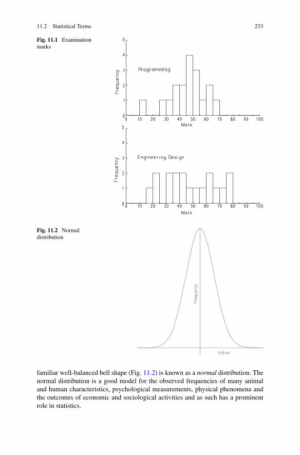
11.2 Statistical Terms 233
Fig. 11.1 Examinationmarks
Fig. 11.2 Normaldistribution
familiar well-balanced bell shape (Fig. 11.2) is known as a normal distribution. Thenormal distribution is a good model for the observed frequencies of many animaland human characteristics, psychological measurements, physical phenomena andthe outcomes of economic and sociological activities and as such has a prominentrole in statistics.
234 11 Statistics
11.2.3 Expected Value, Average and Mean
The expected value of a random variable is defined to be its average value. However,in statistics the term mean is preferred to average, and so we use this term hence-forth. We use E(x) to denote the expected value of a random variable x. Thus if x
is observed to take values x1, x2, . . . , xn we have
E(x) = 1
n
n∑
i=1
xi.
We can extend the definition to define the expected value of a continuous functionf (x) over an interval [a, b]. We divide the interval into n equal sections [xi, xi+1](x1 = a, xn+1 = b) and approximate the area under the curve by the sum of the areasof the rectangles of height f (xi) and width b−a
n. This is a simpler approximation
than that inherent in the trapezium rule of Chap. 5 but it serves our purpose. Wehave
b − a
n
n∑
i=1
f (xi) ≈∫ b
a
f (x) dx
and so in the limit as n tends to infinity
E(f (x)
) = 1
b − a
∫ b
a
f (x) dx. (11.1)
11.2.4 Variance and Standard Deviation
The expected value of a random variable does not necessarily indicate how thevalues are dispersed. For example, a set of examination marks which are bunchedaround the 50% level may have the same average as marks which are more widelydispersed. Quite different conclusions might be drawn from the two sets of results.We introduce variance and standard deviation as measures of the dispersion of a setof values taken by a random variable.
If x is a single random variable having an expected value E(x), the variance,Var(x), of x is defined by
Var(x) = E([
x − E(x)]2)
.
The definition of variance extends to a set of variables x1, x2, . . . xn, with mean valueE(x) and is usually symbolised by σ 2, where
σ 2 = 1
n
n∑
i=1
(xi − E(x)
)2.
11.2 Statistical Terms 235
The standard deviation is defined to be the square root of the variance and so vari-ance is often denoted by σ 2 and standard deviation by σ .
However standard deviation is invariably computed according to the formula
σ =√√√√ 1
n − 1
n∑
i=1
([xi − E(x)
]2). (11.2)
There is a somewhat tortuous statistical justification for using n − 1 rather thann based on the following, which may be tested by experiment to provide a morereliable estimate. The formula is based on the values x1, x2, . . . , xn which are oftenjust a sample of all possible values. For example the xi values may result from asurvey of journey times to work which would have probably been based on a samplegroup of employees. In this case E(x) in the formula is based on just a selection ofall possible xi values and so is not an independent variable. This restriction reducesthe degrees of freedom inherent in the equation from n to n − 1.
The standard deviation indicates where the values of a frequency distribution arelocated in relation to the mean. According to Chebyshev’s theorem at least 75%of values will fall within ±2 times the standard deviation of the mean and at least89% will fall within ±3 times the standard deviation of the mean. For a normaldistribution the proportions of variables falling within 1, 2 and 3 standard deviationsare respectively 68%, 95% and 99%.
Problem
Find the mean and standard deviation of the sets of examination (see Table 11.1)marks from the same group of students. The marks are given in order of studentname. Histograms were shown in Fig. 11.1. Verify that Chebyshev’s theorem holds.
Solution
The mean, Ep , for Programming is given by
Ep = (41 + 42 + 48 + 47 + 49 + 49 + 50 + 52 + 52
+ 14 + 34 + 35 + 37 + 55 + 60 + 67 + 29 + 63)/18
= 45.8.
Table 11.1 Examination marks
Programming
41 42 48 47 49 49 50 52 52 14 34 35 37 55 60 67 29 63
Engineering Design
15 21 22 30 33 37 39 43 43 47 50 56 60 63 67 70 76 79
236 11 Statistics
Table 11.2 Examination marks, Chebyshev analysis
Range No. of marks in the range No. of marks as a percentage
Ep ± 2σp (20.8,70.8) 17 94.4% (> 75%)
Ee ± 2σe (9.8,84.7) 18 100% (> 75%)
In this example we have an accurate evaluation of Ep since we are using resultsfrom the whole group. No estimates are used and so we use n rather than n − 1 inthe denominator of the formula for variance, (11.2).
The standard deviation, σp , for Programming is given by
σp = √([(41 − 45.8)2 + (42 − 45.8)2 + · · · + (63 − 45.8)2]/18
)
= 12.5.
The corresponding figures for Engineering design are Ee = 47.3 and σe = 9.8. Ifwe look at the number of marks within ±2 times the standard deviation of the mean(see Table 11.2) we find that Chebyshev’s theorem holds.
Discussion
It is clear from the histograms shown in Fig. 11.1 that for Programming more stu-dents are bunched around the mean than for Engineering Design. This is reflected inthe very different values of the standard deviations. The greater standard deviationfor Engineering Design indicates the greater spread of marks. Although the two setsof marks have similar mean values this does not fully describe the situation.
11.2.5 Covariance and Correlation
If two sets of random variables x and y are being recorded we define their jointvariance, or covariance, to be Cov(x, y), where
Cov(x, y) = E[(
x − E(x))(
y − E(y))]
.
The formula may be justified by considering the values taken by two random vari-ables x and y. If for example, x1 and y1 vary in the same direction from the respec-tive means E(x) and E(y), they will be contributing a positive product to the sumof terms
n∑
i=1
(xi − E(x)
)(yi − E(x)
)
the larger the magnitude of the product, the stronger the relationship in that partic-ular instance. On the other hand if xi and yi vary in opposite directions from theirrespective means a negative quantity is contributed. If each instance of x, xi behaved
11.2 Statistical Terms 237
in exactly the same way as the corresponding instance yi we would have completeagreement and so the expected value of (x −E(x))(y −E(y)) would be the positivevalue of
√Var(x)Var(y) on the other hand the complete opposite would produce the
negative value. Accordingly we construct a correlation coefficient ρ, where
ρ = Cov(x, y)√Var(x)Var(y)
as a measure of the joint variability of random variables x and y. The coefficientρ may take values between ±1. We speak of variables being highly correlated, oron the other hand of being uncorrelated, depending on the value of their correlationcoefficient ρ.
A value approaching +1 corresponds to the case where the joint variability ishigh. It can be imagined that there is a high correlation between certain life stylesand respiratory and other diseases. On the other hand there would seem to be littlecorrelation between the rainfall in Lancashire and the number of delays on the Lon-don Underground and so a correlation coefficient closer to zero might be expected.A correlation coefficient approaching −1 suggests an inverse relationship. A possi-ble example might be the number of umbrellas purchased in a holiday resort in anyone week against the volume of sun tan lotion. As one goes up, the other is expectedto go down. However, it should be emphasised that a coefficient correlation nearing±1 does not necessarily imply cause and effect. The whole theory is based on in-stances of comparable data. Consideration must be given to the quantity and qualityof data, the order in which data is compared and to the possibility of coincidence.
Problem
In addition to the previous examination marks consider the marks attained in FluidMechanics by the same class. As before the marks are given in order of studentname (Table 11.3). Calculate the correlation coefficients for all possible pairings ofmarks for Programming, Engineering Design and Fluid Mechanics.
Solution
The mean and standard deviation for Fluid Mechanics are found to be 55.6 and 18.6respectively.
The covariance, Cov(f,p), of the marks for Fluid Mechanics and Programmingis found from
Table 11.3 Further examination marks
Fluid Mechanics
11 22 38 39 42 51 54 57 60 66 67 68 73 78 76 80 55 63
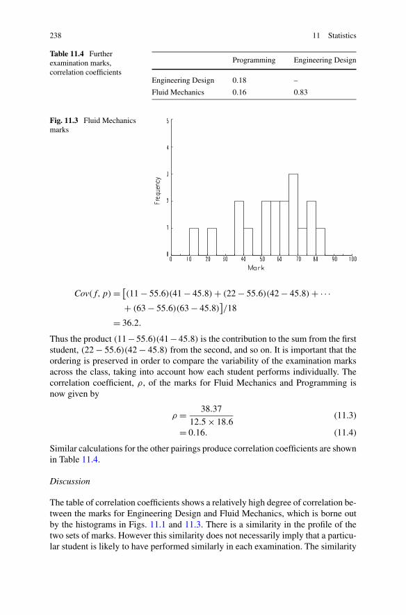
238 11 Statistics
Table 11.4 Furtherexamination marks,correlation coefficients
Programming Engineering Design
Engineering Design 0.18 –
Fluid Mechanics 0.16 0.83
Fig. 11.3 Fluid Mechanicsmarks
Cov(f,p) = [(11 − 55.6)(41 − 45.8) + (22 − 55.6)(42 − 45.8) + · · ·+ (63 − 55.6)(63 − 45.8)
]/18
= 36.2.
Thus the product (11−55.6)(41−45.8) is the contribution to the sum from the firststudent, (22 − 55.6)(42 − 45.8) from the second, and so on. It is important that theordering is preserved in order to compare the variability of the examination marksacross the class, taking into account how each student performs individually. Thecorrelation coefficient, ρ, of the marks for Fluid Mechanics and Programming isnow given by
ρ = 38.37
12.5 × 18.6(11.3)
= 0.16. (11.4)
Similar calculations for the other pairings produce correlation coefficients are shownin Table 11.4.
Discussion
The table of correlation coefficients shows a relatively high degree of correlation be-tween the marks for Engineering Design and Fluid Mechanics, which is borne outby the histograms in Figs. 11.1 and 11.3. There is a similarity in the profile of thetwo sets of marks. However this similarity does not necessarily imply that a particu-lar student is likely to have performed similarly in each examination. The similarity
11.3 Least Squares Analysis 239
may not extend beyond the nature of the examination itself. On the other hand thecorrelation coefficients between the marks for Programming and the other exami-nations are low, indicating that as a whole they have little in common. Again this isborne out by consideration of the histograms. Other things being equal perhaps theProgramming examination was quite different in character from the other two. Thedoor to speculation is open.
11.3 Least Squares Analysis
We return to the problem of fitting a straight line to a given set of data using themethod of least squares first discussed in Chap. 4.
Given data (xi, yi), i = 1, . . . , n the aim is to find coefficients a and b such thatthe straight line y = a + bx, often referred to as the regression line, approximatesthe data in a least squares sense. In general the data which we present to a leastsquares program will be subject to error.
In order to measure the reliability of the approximating straight line we use ameasure known as the standard error estimate, SEE defined by
SEE =√∑n
i=1(yi − yi )2
n − 2
where yi are the approximations to the data values yi calculated using the regressionline yi = a + bxi , i = 1, . . . , n.
Standard deviation was used to measure dispersion about a mean value. The stan-dard error estimate is a measure of dispersion (or scatter) around the regression line.As with standard deviation we take account of the number of degrees of freedomwhen using standard error estimates. In this case the expression is constrained bythe equations for a and b, which are estimates for the actual (and unknown) linearrelationship between the variables x and y. The number of degrees of freedom isreduced by two and so n − 2 appears in the denominator.
Problem
Fit a regression line (i.e. a least squares linear approximation) to the data givenin Table 11.5 using the results from (Chap. 4, question 1) find the standard errorestimate. Identify the data points which lie within 1, 2 and 3 standard errors of theregression line.
Table 11.5 Young’sModulus, data t 0 100 200 300 400 500 600
y 200 190 185 178 170 160 150
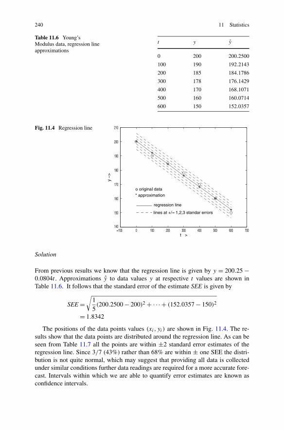
240 11 Statistics
Table 11.6 Young’sModulus data, regression lineapproximations
t y y
0 200 200.2500
100 190 192.2143
200 185 184.1786
300 178 176.1429
400 170 168.1071
500 160 160.0714
600 150 152.0357
Fig. 11.4 Regression line
Solution
From previous results we know that the regression line is given by y = 200.25 −0.0804t . Approximations y to data values y at respective t values are shown inTable 11.6. It follows that the standard error of the estimate SEE is given by
SEE =√
1
5(200.2500 − 200)2 + · · · + (152.0357 − 150)2
= 1.8342
The positions of the data points values (xi, yi) are shown in Fig. 11.4. The re-sults show that the data points are distributed around the regression line. As can beseen from Table 11.7 all the points are within ±2 standard error estimates of theregression line. Since 3/7 (43%) rather than 68% are within ± one SEE the distri-bution is not quite normal, which may suggest that providing all data is collectedunder similar conditions further data readings are required for a more accurate fore-cast. Intervals within which we are able to quantify error estimates are known asconfidence intervals.
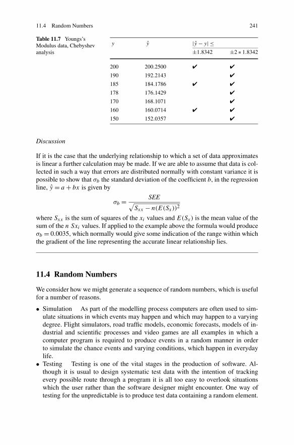
11.4 Random Numbers 241
Table 11.7 Youngs’sModulus data, Chebyshevanalysis
y y |y − y| ≤±1.8342 ±2 ∗ 1.8342
200 200.2500 ✔ ✔
190 192.2143 ✔
185 184.1786 ✔ ✔
178 176.1429 ✔
170 168.1071 ✔
160 160.0714 ✔ ✔
150 152.0357 ✔
Discussion
If it is the case that the underlying relationship to which a set of data approximatesis linear a further calculation may be made. If we are able to assume that data is col-lected in such a way that errors are distributed normally with constant variance it ispossible to show that σb the standard deviation of the coefficient b, in the regressionline, y = a + bx is given by
σb = SEE√Sxx − n(E(Sx))2
where Sxx is the sum of squares of the xi values and E(Sx) is the mean value of thesum of the n Sxi values. If applied to the example above the formula would produceσb = 0.0035, which normally would give some indication of the range within whichthe gradient of the line representing the accurate linear relationship lies.
11.4 Random Numbers
We consider how we might generate a sequence of random numbers, which is usefulfor a number of reasons.
• Simulation As part of the modelling process computers are often used to sim-ulate situations in which events may happen and which may happen to a varyingdegree. Flight simulators, road traffic models, economic forecasts, models of in-dustrial and scientific processes and video games are all examples in which acomputer program is required to produce events in a random manner in orderto simulate the chance events and varying conditions, which happen in everydaylife.
• Testing Testing is one of the vital stages in the production of software. Al-though it is usual to design systematic test data with the intention of trackingevery possible route through a program it is all too easy to overlook situationswhich the user rather than the software designer might encounter. One way oftesting for the unpredictable is to produce test data containing a random element.
242 11 Statistics
• Numerical methods There are problems which may be solved by Monte Carlomethods which build a solution based on a number of random evaluations. Welook at one such method for numerical integration.
11.4.1 Generating Random Numbers
Short of attaching a coin tossing device to the computer the only feasible way ofgenerating random numbers is by means of software based on mathematical for-mulae. Since numbers which are related by a formula can no longer be regardedas being truly random, the term pseudo-random number is introduced, although thepseudo part is often omitted. The skill in constructing such formulae lies in produc-ing sequences which give every appearance of being random. Many have been triedbut eventually found to be wanting in that the sequence degenerates into the samerelatively short repetitive pattern. Ultimately any formula will return to its startingpoint and so the aim is to make that interval (the cycle) sufficiently large so that forall practical purposes it may be considered to be infinite. Such schemes exclude rep-etitions within the cycle, which would be a feature of a genuinely random sequence,but this shortcoming is deemed to be acceptable.
The most popular form of random number generator is the multiplicative con-gruential generator which produces integers using the formula
ni+1 = λni mod m, i = 1,2, . . . (11.5)
λ is known as the multiplier, m is known as the modulus and the starting value n1 isknown as the seed. Successive values are found by calculating the remainder whenλ times the current value of ni is divided by m as shown in the following:
Problem
Generate a sequence of random numbers using the multiplicative congruential gen-erator with multiplier 3, modulus 11 and seed 1.
Solution
Using (11.5) we have
n1 = 1
n2 = remainder[(3 × 1) ÷ 11
] = 3
n3 = remainder[(3 × 3) ÷ 11
] = 9
n4 = remainder[(3 × 9) ÷ 11
] = 5
n5 = remainder[(3 × 5) ÷ 11
] = 4
n6 = remainder[(3 × 4) ÷ 11
] = 1
at which point the cycle 3, 9, 5, 4, 1 repeats.

11.5 Random Number Generators 243
Discussion
Clearly the sequence we are generating could not be considered to be a satisfactoryrandom selection of integers from the range 1 to 10 since 2, 6, 7, 8 and 10 are miss-ing. On the other hand the sequence ni+1 = 3ni mod 19 generates all the integers inthe range 1 to 18.
If a large selection of numbers is required, repetition of relatively short cyclesdestroys all pretence that the sequence is chosen at random. The multiplicative for-mula (11.5) has the potential to generate numbers between 1 and m − 1 and so thehunt is on to find a and m to give sequences which generate most, if not all numbersin the range. Ideally m should be as large as possible so that we have an algorithmto cover all eventualities.
11.5 Random Number Generators
We give two popular generators:
ni+1 = 75ni mod(231 − 1
), i = 1,2, . . . (11.6)
and
ni+1 = 1313ni mod 259, i = 1,2, . . . . (11.7)
Generator (11.6) has the advantage that it may be programmed on most computersusing a high-level language provided care is taken to avoid integer overflow. It hasa cycle length of 231 − 1 (2147483647) and was used in early implementations ofMatlab. It has since been replaced by a different algorithm1 based on multiple seedswith an even longer cycle length of 21430. Generator (11.7) is not so amenable tohigh-level programming since the multiplier and modulus are out of normal integerrange. However it does have a cycle length of 257.
11.5.1 Customising Random Numbers
Floating point random numbers may be produced from an integer random numbergenerator having modulus m, by dividing by m. Using the problem above as anexample, the output as floating point numbers would be 0.2727, 0.8182, 0.4545,0.3636, 0.0909 at which point the cycle repeats. Dividing by the modulus, m en-sures that numbers produced lie within the range (0,1), but results may be scaledto lie within any desired range. See the exercises for further details including theproduction of random integers.
1For details see http://www.mathworks.com/moler/random.pdf.
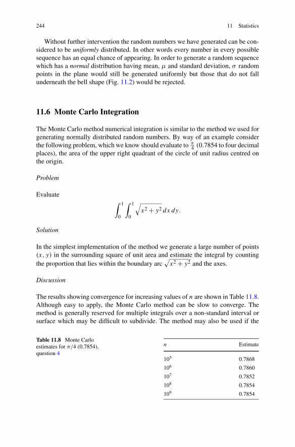
244 11 Statistics
Without further intervention the random numbers we have generated can be con-sidered to be uniformly distributed. In other words every number in every possiblesequence has an equal chance of appearing. In order to generate a random sequencewhich has a normal distribution having mean, μ and standard deviation, σ randompoints in the plane would still be generated uniformly but those that do not fallunderneath the bell shape (Fig. 11.2) would be rejected.
11.6 Monte Carlo Integration
The Monte Carlo method numerical integration is similar to the method we used forgenerating normally distributed random numbers. By way of an example considerthe following problem, which we know should evaluate to π
4 (0.7854 to four decimalplaces), the area of the upper right quadrant of the circle of unit radius centred onthe origin.
Problem
Evaluate∫ 1
0
∫ 1
0
√x2 + y2 dx dy.
Solution
In the simplest implementation of the method we generate a large number of points(x, y) in the surrounding square of unit area and estimate the integral by countingthe proportion that lies within the boundary arc
√x2 + y2 and the axes.
Discussion
The results showing convergence for increasing values of n are shown in Table 11.8.Although easy to apply, the Monte Carlo method can be slow to converge. Themethod is generally reserved for multiple integrals over a non-standard interval orsurface which may be difficult to subdivide. The method may also be used if the
Table 11.8 Monte Carloestimates for π/4 (0.7854),question 4
n Estimate
105 0.7868
106 0.7860
107 0.7852
108 0.7854
109 0.7854

11.6 Monte Carlo Integration 245
integrand or its derivatives have discontinuities that invalidate some of the assump-tions inherent in the more formal methods of Chap. 5.
Summary This chapter has been a somewhat cursory introduction to statistics.You will have become familiar with a number of technical terms and will be able toappreciate their significance when they are used in other contexts.
We have dealt with the problem of using a computer to generate random num-bers. We explained the need for such a facility and showed by example that a mul-tiplicative congruential generator could be used to good effect. We used the aptlynamed Monte Carlo method to add to the methods for numerical integration givenin Chap. 5.
Exercises
1. Use the following segments of code in a program to explore further plottingfacilities of Matlab and to verify the results of Sects. 11.2.4 and 11.2.5 usinga selection of the Matlab statistical routines hist (histogram), bar (bar chart),mean (mean), std (standard deviation) and cov (covariance). By default graphswill appear in the Matlab Fig. 1 window, which should be kept in view. Becauseof the usually more applicable formula (11.2) that Matlab uses for calculatingstandard deviations, results may differ slightly form those quoted in the chapter.
%% Create vectors p, e and f to contain the marks% for Programming, Engineering Design and Fluid Mechanics%% basic histogram for the Fluid Mechanics
hist(e)% set the number of columns to 5, store the number of marks in each column% in the vector n
% column locations are recorded in cen.%
[n cen] = hist(e, 5);%% Plot the histogram as a bar chart%
bar(cen, n, 'r') % set the bar colour to r red, (Sect. 1.13)axis([10 100 0 6]) % set axes limitsset(gca,'YTick', 0 : 1 : 6) % set the tick marks on the Y axis
% gca is a Matlab abbreviation for get current axisgtext('Fluid Mechanics'); % add the title interactively by moving
% the cross-hairs and clickingxlabel('Mark'); % label the x-axisylabel('Frequency'); % label the y-axis
%
246 11 Statistics
% Calculate mean values and standard deviations, for example:%
mean(p)std(p)
%% Find the covariance of for example Programming v. Engineering Design.% cov returns a symmetric 2 × 2 matrix with diagonal elements equal to% the standard deviations of p and e respectively. The covariance% is given by the off diagonal element.
X = cov(p, e)% The correlation coefficient is given by
X(1,2)/(sqrt(X(1,1)∗X(2,2)))
2. (i) Write a program to verify the results quoted in Sect. 11.3 relating to fitting theregression line.
(ii) Repeat the program using data for the gas problem as quoted in Table4.1, Chap. 4. Verify that the standard error estimate, SEE is 0.2003 and that thestandard deviation of the regression coefficient, σb is 0.0958.
Although the SEE value found in case (i) (1.8342) is larger than for case (ii)it should be remembered that in (i) we were dealing with data values of an order102 higher. Scaling the result from (i) by 10−2 shows the SEE to be smaller by afactor of 10, which is to be expected since the relationship between gas pressureand volume was seen to be essentially non-linear (Fig. 4.1, Chap. 4).
3. (i) Write a program to generate 20 random numbers in the range (0,1) usingformula 11.6. Choose your own seed in the range (2,231 − 1) but use a largenumber (for example 123456). You will see by experimenting that a small seedwill produce what might be considered to be an unsatisfactory random selection.
(ii) Modify the program so that the 20 random numbers in the range (−1,1)
are produced. Use the formula 2x − 1 on numbers x randomly produced in therange (0,1).
(iii) Modify the program so that the 10 random integers in the range (5,100)
are produced. Use the formula 95x + 5 on numbers x in the range (0,1) to pro-duce values in the range (5,100) and then take the highest integer number belowthe random value using the Matlab floor function.
Matlab provides a variety of routines for generating random numbers. In par-ticular the functions random and randint, which may be used to answer parts(i)–(iii) of the question can take many forms as shown by the following state-ments:
% generate a single number in the range (a, b) from a uniform distributionr = random('unif ', a, b) ;
% as above but numbers generated in an m by n matrix from the range (a, b)A = random('unif ', a, b, m, n);
% generate an m by n matrix of integers in the range (a, b)A = randint(m, n, [a b]);

11.6 Monte Carlo Integration 247
By default seeds are set automatically in all Matlab functions generating randomnumbers and will vary from one execution of a program to another. Howeverthere are facilities for programmers to set specific seeds.
4. Write a program to verify the results quoted in the chapter for Monte Carlo in-tegration. Estimate the area by generating a given number, n of random points(x, y) drawn from a uniform distribution of x and y values in the range (0,1.0).All (x, y) points will lie within a rectangle of area equal to 1. As points are gen-erated count the numbers of pairs which are less than or equal to
√x2 + y2, n1
and those which are greater, n2. The area of the quadrant will be approximatelyn1/(n1 + n2).
5. The equation of the bell-shape enclosing points (x, y) over the range (−∞ <
x < ∞) having normal distribution having zero mean and standard deviation, σ
has the form
y = A exp
(−x2
2σ 2
)
where A is a constant. In practice a smaller range may be considered as y val-ues fall rapidly and to all intents and purposes become zero as x values movesufficiently far away from the origin.
Consider the special case, A = 1 and σ = 0.5. Find the area under the curvefor values of x in the three ranges |xi | ≤ i σ , i = 1,2,3. Use the same techniqueas in the previous question to estimate the areas by generating a given number,N of random points (x, y) drawn from a uniform distribution of x values in therange (−3,3) and y values in the range (0,1). All (x, y) points will lie within arectangle of area equal to 6. There is little point in sampling outside this rangeof x values since y(±3) is of order 1.5e-8 and decreasing rapidly As points aregenerated count the number in each of the three groups
y ≤ exp(−2x2) and (i) |x| ≤ 0.5, (ii) |x| ≤ 1.0, (iii) |x| ≤ 1.5.
If the final totals are n1, n2 and n3, the corresponding areas will be approximately3ni/N , i = 1,2,3. Table 11.9 shows the (very slow) progress of the iteration forincreasing n. Write a program to verify the results shown in Table 11.9.
Express areas (i), (ii) and (iii) as fractions of the whole area enclosed by thebell-shape and the axis to show values consistent with a normal distribution.
Table 11.9 Monte Carloestimates for the bell-shape,question 5
N Area (i) Area (ii) Area (iii)
104 1.24 1.19 0.84
105 1.23 1.18 0.85
106 1.25 1.20 0.85
107 1.25 1.20 0.86
108 1.25 1.20 0.86
248 11 Statistics
Given the decreasing nature of y the integral, the relevant area under the curvenamely,
∫ +3
−3exp
(−2x2)dx.
may be approximated using the standard result∫ +∞
−∞exp
(−2x2)dx =√
π
2.
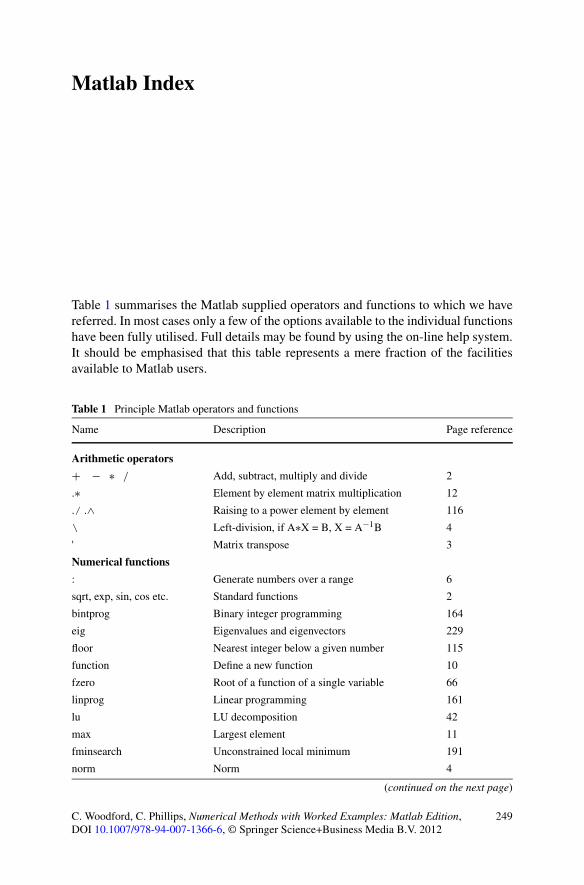
Matlab Index
Table 1 summarises the Matlab supplied operators and functions to which we havereferred. In most cases only a few of the options available to the individual functionshave been fully utilised. Full details may be found by using the on-line help system.It should be emphasised that this table represents a mere fraction of the facilitiesavailable to Matlab users.
Table 1 Principle Matlab operators and functions
Name Description Page reference
Arithmetic operators
+ − ∗ / Add, subtract, multiply and divide 2
.∗ Element by element matrix multiplication 12
./ .∧ Raising to a power element by element 116
\ Left-division, if A∗X = B, X = A−1B 4
' Matrix transpose 3
Numerical functions
: Generate numbers over a range 6
sqrt, exp, sin, cos etc. Standard functions 2
bintprog Binary integer programming 164
eig Eigenvalues and eigenvectors 229
floor Nearest integer below a given number 115
function Define a new function 10
fzero Root of a function of a single variable 66
linprog Linear programming 161
lu LU decomposition 42
max Largest element 11
fminsearch Unconstrained local minimum 191
norm Norm 4
(continued on the next page)
C. Woodford, C. Phillips, Numerical Methods with Worked Examples: Matlab Edition,DOI 10.1007/978-94-007-1366-6, © Springer Science+Business Media B.V. 2012
249
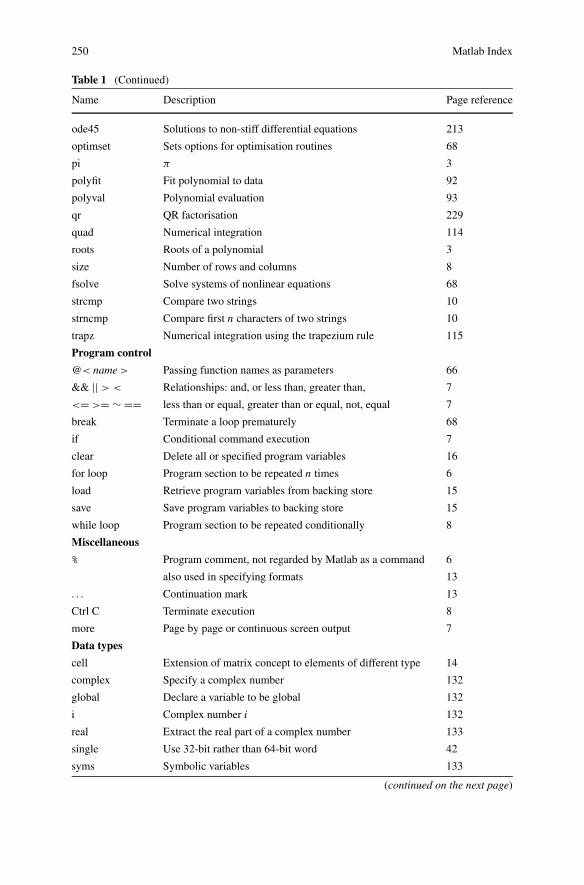
250 Matlab Index
Table 1 (Continued)
Name Description Page reference
ode45 Solutions to non-stiff differential equations 213
optimset Sets options for optimisation routines 68
pi π 3
polyfit Fit polynomial to data 92
polyval Polynomial evaluation 93
qr QR factorisation 229
quad Numerical integration 114
roots Roots of a polynomial 3
size Number of rows and columns 8
fsolve Solve systems of nonlinear equations 68
strcmp Compare two strings 10
strncmp Compare first n characters of two strings 10
trapz Numerical integration using the trapezium rule 115
Program control
@< name > Passing function names as parameters 66
&& || > < Relationships: and, or less than, greater than, 7
<= >= ∼ == less than or equal, greater than or equal, not, equal 7
break Terminate a loop prematurely 68
if Conditional command execution 7
clear Delete all or specified program variables 16
for loop Program section to be repeated n times 6
load Retrieve program variables from backing store 15
save Save program variables to backing store 15
while loop Program section to be repeated conditionally 8
Miscellaneous
% Program comment, not regarded by Matlab as a command 6
also used in specifying formats 13
. . . Continuation mark 13
Ctrl C Terminate execution 8
more Page by page or continuous screen output 7
Data types
cell Extension of matrix concept to elements of different type 14
complex Specify a complex number 132
global Declare a variable to be global 132
i Complex number i 132
real Extract the real part of a complex number 133
single Use 32-bit rather than 64-bit word 42
syms Symbolic variables 133
(continued on the next page)
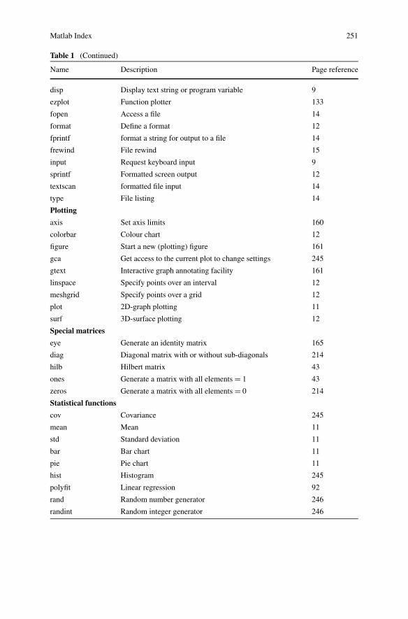
Matlab Index 251
Table 1 (Continued)
Name Description Page reference
disp Display text string or program variable 9
ezplot Function plotter 133
fopen Access a file 14
format Define a format 12
fprintf format a string for output to a file 14
frewind File rewind 15
input Request keyboard input 9
sprintf Formatted screen output 12
textscan formatted file input 14
type File listing 14
Plotting
axis Set axis limits 160
colorbar Colour chart 12
figure Start a new (plotting) figure 161
gca Get access to the current plot to change settings 245
gtext Interactive graph annotating facility 161
linspace Specify points over an interval 12
meshgrid Specify points over a grid 12
plot 2D-graph plotting 11
surf 3D-surface plotting 12
Special matrices
eye Generate an identity matrix 165
diag Diagonal matrix with or without sub-diagonals 214
hilb Hilbert matrix 43
ones Generate a matrix with all elements = 1 43
zeros Generate a matrix with all elements = 0 214
Statistical functions
cov Covariance 245
mean Mean 11
std Standard deviation 11
bar Bar chart 11
pie Pie chart 11
hist Histogram 245
polyfit Linear regression 92
rand Random number generator 246
randint Random integer generator 246
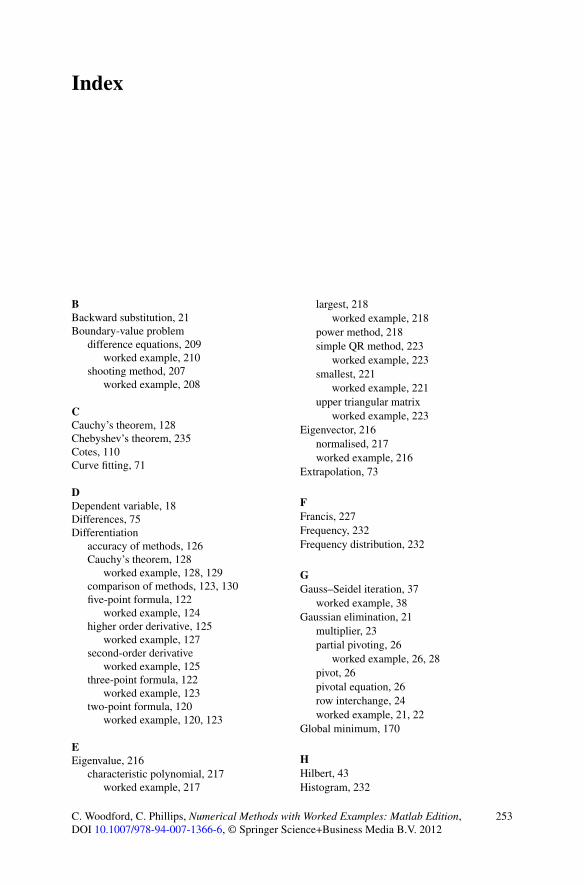
Index
BBackward substitution, 21Boundary-value problem
difference equations, 209worked example, 210
shooting method, 207worked example, 208
CCauchy’s theorem, 128Chebyshev’s theorem, 235Cotes, 110Curve fitting, 71
DDependent variable, 18Differences, 75Differentiation
accuracy of methods, 126Cauchy’s theorem, 128
worked example, 128, 129comparison of methods, 123, 130five-point formula, 122
worked example, 124higher order derivative, 125
worked example, 127second-order derivative
worked example, 125three-point formula, 122
worked example, 123two-point formula, 120
worked example, 120, 123
EEigenvalue, 216
characteristic polynomial, 217worked example, 217
largest, 218worked example, 218
power method, 218simple QR method, 223
worked example, 223smallest, 221
worked example, 221upper triangular matrix
worked example, 223Eigenvector, 216
normalised, 217worked example, 216
Extrapolation, 73
FFrancis, 227Frequency, 232Frequency distribution, 232
GGauss–Seidel iteration, 37
worked example, 38Gaussian elimination, 21
multiplier, 23partial pivoting, 26
worked example, 26, 28pivot, 26pivotal equation, 26row interchange, 24worked example, 21, 22
Global minimum, 170
HHilbert, 43Histogram, 232
C. Woodford, C. Phillips, Numerical Methods with Worked Examples: Matlab Edition,DOI 10.1007/978-94-007-1366-6, © Springer Science+Business Media B.V. 2012
253

254 Index
IIEEE standards, 26Independent variable, 18Initial-value problem
Euler’s method, 200worked example, 200
Runge–Kutta, 202, 204, 206worked example, 202, 205, 206
Integer programming, 136, 149branch and bound, 150
worked example, 151continuous problem, 150decision problem, 153
decision variable, 154worked example, 154
the machine scheduling problem, 156worked example, 156
the travelling salesman problem, 155worked example, 155
Integrand, 97Integration
adaptive quadrature, 112worked example, 112
comparison of methods, 109, 114Gaussian quadrature, 110
worked example, 111higher order rules, 109Monte Carlo, 244
worked example, 244Newton Cotes, 109
three-eighths rule, 109of analytic function, 104
worked example, 108of irregularly tabulated function, 102
worked example, 102of tabulated function, 98
worked example, 98Simpson’s rule, 101, 106
worked example, 101trapezium rule, 99, 101, 104
worked example, 99Integration by parts, 98Interpolating polynomial
comparison of methods, 81Neville, 80
worked example, 80Newton, 77
worked example, 78, 79spline, 82
worked example, 84Interpolation
inverse, 73Lagrange, 108linear, 72
piecewise, 84worked example, 72
piecewise linear, 74polynomial, 77
piecewise (spline), 84Iterative refinement, 35
residual, 36worked example, 35
JJosephson junction, 198
LLagrangian, 187Least squares approximation, 85
confidence interval, 240linear, 86
worked example, 86normal equations, 88polynomial, 88, 91
worked example, 89residual, 86
Legendre polynomial, 110Linear approximation, 72Linear dependence, 33Linear equation
comparison of methods, 38Linear programming, 135
basic variables, 144canonical form, 140, 141
worked example, 141constraints, 135costs, 140dual problem, 146feasible region, 138feasible vertex, 142graphical method, 138
worked example, 138objective, 135optimal solution, 136problem variables, 140simplex method, see separate entry, 142slack variables, 141standard form, 141
worked example, 141trivial constraints, 138vertex, 140
Linear relation, 18example
Hooke’s law, 18Kirchoff’s law, 18mercury thermometer, 18
Linear system, 18as a model of physical processes, 20banded, 211
Index 255
Linear system (cont.)example
portal frame, 20ill-conditioned, 37in matrix–vector form, 19
worked example, 19infinity of solutions, 32
worked example, 32multiple right hand sides, 30
worked example, 30no solution, 32
worked example, 32no unique solution, 32
worked example, 32overdetermined, 86singular, 33sparse, 211symmetric positive definite, 33
worked example, 33upper triangular system, 20
worked example, 20Local minimum, 170
comparison of methods, 174, 181constrained variables, 184golden section search, 172
worked example, 173grid search, 171
worked example, 171method of steepest descent, 176
worked example, 176multiplier penalty function method, 186
worked example, 188penalty function method, 185
worked example, 185rank-one method, 178
worked example, 179rank-two method, 184single variable, 171
LU decomposition, 24
MMatrix
coefficient matrix, 19determinant, 217diagonally dominant, 35Jacobian, 63permutation matrix, 28singular, 33sparse, 38symmetric positive definite, 33unitary, 229upper triangular, 21
Mean value theorem, 60Mixed integer programming, 136
NNatural vibration, 216Nonlinear equation
bisection method, 48worked example, 49
comparison of methods, 58example
Butler–Volmer, 48Newton–Raphson method
problems, 58worked example, 56
rule of false position, 51worked example, 51
secant method, 52breakdown, 54worked example, 52
Nonlinear system, 58example
metal plate, 59turbine rotor, 63
Newton’s method, 58worked example, 59, 63
Normal distribution, 233
OOperations research, 159Order of convergence, 58Ordinary differential equation, 198
boundary-value problem, see separateentry, 199
comparison of methods, 203first-order, 198higher order equations, 207initial-value problem, see separate entry,
199local truncation error, 205nth-order, 199second-order, 199
PPseudo-random number, 242
generator, 242multiplicative congruential, 242
RRandom number, see also pseudo-random
number, 241Random variable, 232
average, 233correlation, 236
worked example, 237covariance, 236dispersion, 234expected value, 233

256 Index
Random variable (cont.)mean, 233mean and standard deviation
worked example, 235standard deviation, 234variance, 234
Raphson, 47Regression, 239
standard error estimate, 239worked example, 239
Root, 47Rounding error, 26
SSimilarity transformation, 223
Simplex methodall slack solution, 144artificial variable, 148basic feasible solution, 144non-basic variables, 143pseudo objective, 147revised simplex method, 146worked example, 142, 144, 147, 148
Stochastic variable, 232
TTaylor series, 120, 179, 204
ZZero (of a function), 47