numerical modeling of rogue waves in coastal waters - … · numerical modeling of rogue waves in...

Nat. Hazards Earth Syst. Sci., 14, 861–870, 2014www.nat-hazards-earth-syst-sci.net/14/861/2014/doi:10.5194/nhess-14-861-2014© Author(s) 2014. CC Attribution 3.0 License.

Natural Hazards and Earth System

SciencesO

pen Access

Numerical modeling of rogue waves in coastal waters

A. Sergeeva1,2, A. Slunyaev1,2, E. Pelinovsky3,4, T. Talipova1,2, and D.-J. Doong5

1Institute of Applied Physics, Nizhny Novgorod, Russia2Nizhny Novgorod State Technical University, Nizhny Novgorod, Russia3National Research University, Higher School of Economics, Nizhny Novgorod, Russia4Johannes Kepler University, Linz, Austria5National Taiwan Ocean University, Keelung, Taiwan

Correspondence to:A. Sergeeva ([email protected])

Received: 6 September 2013 – Published in Nat. Hazards Earth Syst. Sci. Discuss.: 22 October 2013Revised: 5 February 2014 – Accepted: 25 February 2014 – Published: 14 April 2014

Abstract. Spatio-temporal evolution of rogue waves mea-sured in Taiwanese coastal waters is reconstructed by meansof numerical simulations. Their lifetimes are up to 100 s.The time series used for reconstructions were measured atdimensionless depths within the range ofkh = 1.3− 4.0,wherek is the wave number andh is the depth. All iden-tified rogue waves are surprisingly weakly nonlinear. Thevariable-coefficient approximate evolution equations, whichtake into account the shoaling effect, allow us to analyzethe abnormal wave evolution over non-uniform real coastalbathymetry. The shallowest simulated point is characterizedby kh ≈ 0.7. The reconstruction reveals an interesting pe-culiarity of the coastal rogue events: though the mean waveamplitudes increase as waves travel onshore, rogue waves arelikely to occur at deeper locations, but not closer to the coast.

1 Introduction

This paper is dedicated to the analysis of rogue waves reg-istered by buoys near the coast of Taiwan and to reproduc-tion of these events with the help of hydrodynamic equations.The long-term measurements of the surface displacement byseveral buoys moored at different locations around Taiwanresulted in a collection of time series characterizing waveconditions in Taiwanese coastal waters (Lee et al., 2011).This data set was analyzed in Doong et al. (2012); in partic-ular, rogue waves (the heights of which at least twice exceedthe background significant wave height) have been identifiedand analyzed. The rogue (or freak) waves are a threat thathas been recognized rather recently, and nowadays attracts

much attention (see Kharif and Pelinovsky, 2003; Dysthe etal., 2008; Kharif et al., 2009; Slunyaev et al., 2011, for re-views).

Measurements of the surface elevation at a certain pointprovide only limited information about waves. The resultingtime series, even if they contain rogue waves, do not reflectthe dynamics of these dangerous waves. Much more infor-mation can be derived by merging the measured data withquite reasonable assumptions of wave dynamics. A com-mon assumption is that waves propagate almost unidirection-ally in a wind sea and particularly in swells. This impliesthat the angular spectrum is narrow. It is sufficient to ful-fill this requirement within some reasonably short period oftime, for example, for the duration of surface elevation record(10–20 min), or even shorter. Also, it is often true that thewave system contains no components (for example, reflectedwaves) propagating against the highest waves. Under theseassumptions the surface wave dynamics can be consideredas one-dimensional, for which the boundary value problembecomes in principle treatable. Numerical reconstruction ofthe evolution of such wave systems on the basis of instru-mental records was performed in Trulsen (2001), Divinsky etal. (2004), Slunyaev et al. (2005, 2014), and Slunyaev (2006)by means of approximate evolution equations for modulatedwaves. As a result, not only can much more detailed waveinformation in the vicinity of the measurement point be ob-tained, but also the rogue wave evolution can be recovered.Importantly, application of the weakly nonlinear theory forwave modulations is able to produce reliable results evenfor very steep modulated waves (Slunyaev et al., 2014). A

Published by Copernicus Publications on behalf of the European Geosciences Union.

862 A. Sergeeva et al.: Numerical modeling of rogue waves in coastal waters

Table 1.Main parameters of the in situ records.

h [m] −x0 kph Tp Tfr λfr Hfr H crfr Hs Ur BFI

[km] [s] [s] [m] [m] [m] [m]

1. Hsinchu 26.5 2.5 1.34 9.5 8.8 122 6.2 2.7 3.0 1.26−0.0222. Hualien 30 1 1.9 8.1 7.3 99 3.2 1.7 1.4 0.24 0.0323. Eluanbi 40 2 2.3 8.5 7.3 111 3.4 1.5 1.4 0.14 0.0504. Longdong 42 1 4.0 6.5 6.3 66 2.8 1.6 1.3 0.04 0.136

credible reconstruction of the wave dynamics was possiblefor about 10 min.

An important feature of the measured time series, whichare in the focus of the present paper, is variable bathymetry:the sea is considered as a finite-depth basin, and the depthvariation is essential. The complicated picture of changesin nonlinear waves when they travel from deep to shallowwater was revealed by Sergeeva et al. (2011), Zeng andTrulsen (2012), and Trulsen et al. (2012). Though nonlin-ear wave interactions in constant-depth water are believed totrigger more rogue waves than predicted by the linear quasi-Gaussian statistics, these publications proved that variable-depth conditions were able to further increase the probabilityof rogue waves.

In this paper we consider four time series that are mea-sured in the coastal waters of Taiwan and that contain roguewaves. In order to understand the nonlinear dynamics of ex-treme waves approaching from the open sea to the coast andto assess the rogue wave danger at the coast, we reconstructthe wave evolution of the in situ measured rogue waves em-ploying the nonlinear theory for modulated waves. In Sect. 2the conditions of measurements and the field data are brieflydescribed. The employed evolution equations and the proce-dure of using the in situ time series to initialize the simulationare introduced in Sect. 3. Section 4 provides the results of thesimulations. The outcome is summarized in Discussion.

2 Field data

Long-term instrumental measurements of waves near thecoasts of Taiwan have been conducted since 1997 by Tai-wanese Central Weather Bureau (CWB) and Water Re-sources Agency (WRA) (Doong et al., 2007). Currently thereare 15 buoys in operation in Taiwanese waters. The recordsused in this study are retrieved from four buoys moored atseveral locations, which differ in the distance from the coast,local depth, currents, typical wave spectra, etc. The samplingrate of the buoys is 2 Hz. The 512 s-long sections of time se-ries of surface elevations are produced from the raw data ofbuoy accelerations with use of wavelet transform (see detailsin Lee et al., 2011). An extensive analysis of the availabledata set (Chang, 2012) exhibits a rich variety of rogue waveappearances. There are more than 100 rogue waves measuredat each of those buoys. The occurrence probability of rogue

15

434

Table 1. Main parameters of the in-situ records 435

436

h [m] –x0

[km]

kph Tp [s] Tfr [s] fr [m] Hfr [m] Hfrcr

[m]

Hs [m] Ur BFI

1. Hsinchu 26.5 2.5 1.34 9.5 8.8 122 6.2 2.7 3.0 1.26 -0.022

2. Hualien 30 1 1.9 8.1 7.3 99 3.2 1.7 1.4 0.24 0.032

3. Eluanbi 40 2 2.3 8.5 7.3 111 3.4 1.5 1.4 0.14 0.050

4. Longdong 42 1 4.0 6.5 6.3 66 2.8 1.6 1.3 0.04 0.136

437

438

439

440

441

442

Figure 1. Locations of the buoys used in this study. 443

Fig. 1.Locations of the buoys used in this study.

waves is in the range of 1.7–2.1× 10−4; that is, one roguewave occurs in every 5000 waves. During the presence of atyphoon (tropical cyclone) close to the station, the frequencyof occurrence of rogue waves increased by 2–7 times com-pared to its average level. It was also found that the percent-age of rogue waves with symmetric shapes is large.

Four samples of the time series from the data set werepicked out for the present study (see Figs. 1 and 2). We usedthe conventional criterion for individual rogue waves,

AI ≡H

Hs> 2, (1)

whereH is the height of a single wave andHs is the sig-nificant wave height. Note that we consider short segmentsof surface elevations (about 8.5 min instead of conventional20 min), which may result in some overestimation ofHs, andhence may lead to ignoring some rogue events. The quantity

Nat. Hazards Earth Syst. Sci., 14, 861–870, 2014 www.nat-hazards-earth-syst-sci.net/14/861/2014/

A. Sergeeva et al.: Numerical modeling of rogue waves in coastal waters 863

16

a) 50 100 150 200 250 300 350 400 450 500

−4

−2

0

2

4

Surf

ace

Ele

vati

on [

m]

Time [s] 444

b) 50 100 150 200 250 300 350 400 450 500

−2

−1

0

1

2

Surf

ace

Ele

vati

on [

m]

Time [s] 445

c) 50 100 150 200 250 300 350 400 450 500

−2

−1

0

1

2

Surf

ace

Ele

vati

on [

m]

Time [s] 446

d) 50 100 150 200 250 300 350 400 450 500

−2

−1

0

1

2

Surf

ace

Ele

vati

on [

m]

Time [s] 447

448

Figure 2. Instrumental time series containing rogue waves at a) Hsinchu, b) Hualien, 449

c) Elaunbi, d) Longdong. 450

Fig. 2. Instrumental time series containing rogue waves at(a) Hsinchu,(b) Hualien,(c) Elaunbi, and(d) Longdong.

AI will be referred to as abnormality index, which charac-terizes the deviation of the wave height from the signifi-cant value. The rogue waves represent three kinds of wavegeometry: so-called “holes in the sea” with characteristicdeep troughs (Fig. 2a, c, Hsinchu and Eluanbi stations), sign-variable waves (Fig. 2b, Hualien station) and high-crestedwaves (Fig. 2d, Longdong station). The distances to shore,−x0, for the measuring stations are given in Table 1 togetherwith the local depthh and other related parameters. Periodsof the rogue waves areTfr = 6–10 s, where the subscript frwill denote the rogue (or freak) wave characteristics. Thepeak periods,Tp, are obtained from the frequency spectra,whereas every record contains from 53 to 78 periodsTp.Three buoys out of four are located at intermediate depthswith dimensionless depths,kph, within the range 1.3–2.3.The fourth buoy (Longdong) is moored at a deeper locationwith kph = 4. Herekp is determined from the peak angularfrequency,ωp, through the dispersion relation for finite-depthgravity waves,

ω2= gktanh(kh) . (2)

The significant wave heights, rogue wave heights and crestheights,Hcr, are given in Table 1. The characteristic wavesteepness, estimated from the standard deviationηrms of thesurface elevation, asε = kpηrms, varies from 0.02 to 0.04,which corresponds to rather weak nonlinearity. The steep-ness of the rogue wave may be estimated with the help ofthe local wave lengthλfr (which is related to the local zero-crossing wave period according to the dispersion relationEq. 2) and the crest height. The steepness of identified roguewaveskfrHcr is from 0.08 to 0.15. Therefore, the identifiedrogue waves were essentially weakly nonlinear.

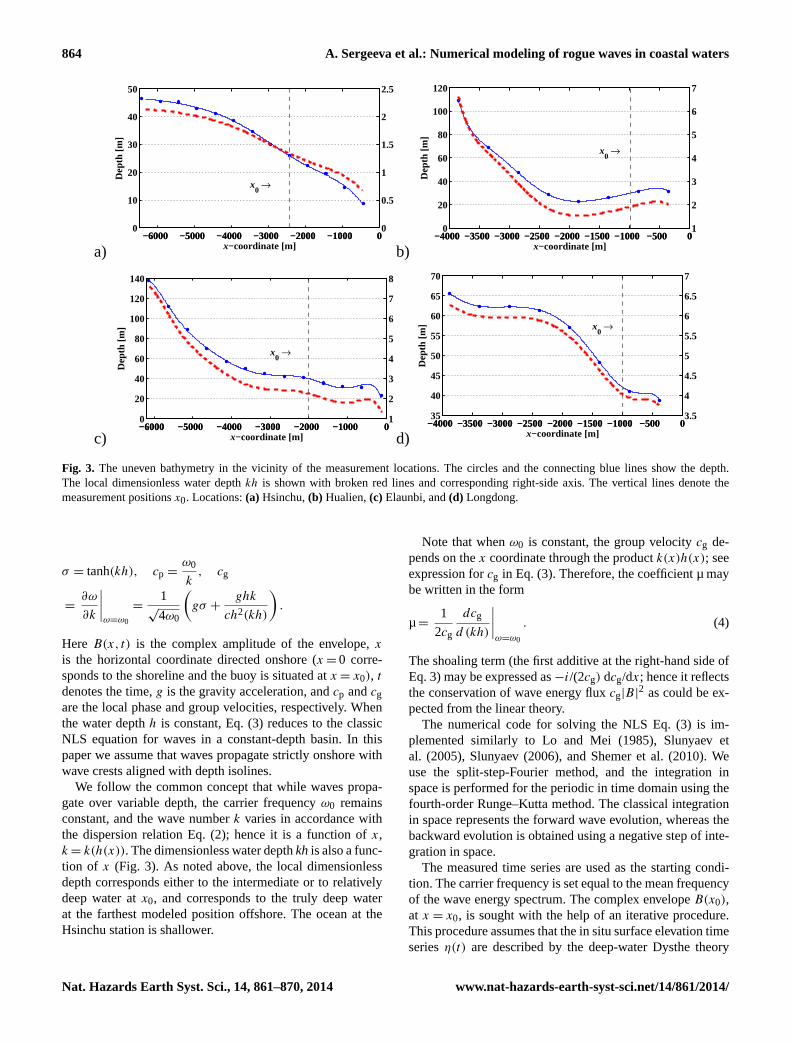
We used realistic bathymetry for numerical simulations ofthe wave propagation both onshore and offshore of the buoylocations. For each buoy the bathymetry was provided at afew locations (see blue circles in Fig. 3 and axis from the leftside of the panels for the depth values) and was interpolatedfor our purposes using polynomial functions.

3 Simulation of weakly nonlinear waves overvariable bottom

The time series of surface elevation, measured by individ-ual gauges, contain very limited information. They basicallypresent the local, instantaneous reaction of the water sur-face to the passing waves, but the wave dynamics remainsconcealed. To reconstruct the wave evolution in the vicin-ity of the measurement point, we employ weakly nonlin-ear equations that are able to describe the transformation ofwaves propagating in one direction (shoreward) over variablebathymetry. A suitable model is the nonlinear Schrödingerequation (NLS) for the case of wave evolution in space overuneven depth. The impact of bathymetry is taken into ac-count through depth-dependent coefficients and a shoalingterm (Djordjevic and Redekopp, 1978; Zeng and Trulsen,2012):

idB

dx= −iµ

d(kh)

dxB −

i

cg

dB

dt+ λ

d2B

dt2+ ν |B|

2B, (3)

µ=

(1− σ 2

)(1− khσ)

σ + kh(1− σ 2),

λ =1

2cgω0

[1−

gh

c2g

(1− khσ)(1− σ 2

)],

ν =ω0k

2

16σ 2cg

[9− 10σ 2

+ 9σ 4−

2σ 2c2g

(gh − c2g)(

4c2

p

c2g

+ 4c2

p

c2g(1− σ 2) +

gh

c2g

(1− σ 2)2

)],

www.nat-hazards-earth-syst-sci.net/14/861/2014/ Nat. Hazards Earth Syst. Sci., 14, 861–870, 2014


17

451

a) −6000 −5000 −4000 −3000 −2000 −1000 0

0

10

20

30

40

50

Dep

th [

m]

x−coordinate [m]

x0 →

−6000 −5000 −4000 −3000 −2000 −1000 00

0.5

1

1.5

2

2.5

b) −4000 −3500 −3000 −2500 −2000 −1500 −1000 −500 0

0

20

40

60

80

100

120

Dep

th [

m]

x−coordinate [m]

x0 →

−4000 −3500 −3000 −2500 −2000 −1500 −1000 −500 01

2

3

4

5

6

7

452

c) −6000 −5000 −4000 −3000 −2000 −1000 00

20

40

60

80

100

120

140

Dep

th [

m]

x−coordinate [m]

x0 →

−6000 −5000 −4000 −3000 −2000 −1000 01

2

3

4

5

6

7

8

d) −4000 −3500 −3000 −2500 −2000 −1500 −1000 −500 035

40

45

50

55

60

65

70

Dep

th [

m]

x−coordinate [m]

x0 →

−4000 −3500 −3000 −2500 −2000 −1500 −1000 −500 03.5

4

4.5

5

5.5

6

6.5

7

453

454

Figure 3. The uneven bathymetry in the vicinity of the measurement locations. The circles and 455

the connecting blue lines show the depth. The local dimensionless water depth kh is shown 456

with broken red lines and corresponding right-side axis. The vertical lines denote the 457

measurement positions x0. Locations: a) Hsinchu, b) Hualien, c) Elaunbi, d) Longdong. 458

459

0 50 100 150 200 250 300 350 400 450 500

−2469

−2427 −2401

−2359

−2317

−2279

−2241 −2207

−2159 −2127

−2089

−2051

−2007 −1975

−1937 −1913

Time [s] 460

Figure 4. The simulated rogue wave evolution in the vicinity of the Hsinchu buoy. Numbers 461

at the left side give values of x in meters. The thick red curves show rogue wave according to 462

Eq. (1) for local x. 463

Fig. 3. The uneven bathymetry in the vicinity of the measurement locations. The circles and the connecting blue lines show the depth.The local dimensionless water depthkh is shown with broken red lines and corresponding right-side axis. The vertical lines denote themeasurement positionsx0. Locations:(a) Hsinchu,(b) Hualien,(c) Elaunbi, and(d) Longdong.

σ = tanh(kh), cp =ω0

k, cg

=∂ω

∂k

∣∣∣∣ω=ω0

=1

√4ω0

(gσ +

ghk

ch2(kh)

).

Here B(x, t) is the complex amplitude of the envelope,x

is the horizontal coordinate directed onshore (x = 0 corre-sponds to the shoreline and the buoy is situated atx = x0), t

denotes the time,g is the gravity acceleration, andcp andcgare the local phase and group velocities, respectively. Whenthe water depthh is constant, Eq. (3) reduces to the classicNLS equation for waves in a constant-depth basin. In thispaper we assume that waves propagate strictly onshore withwave crests aligned with depth isolines.

We follow the common concept that while waves propa-gate over variable depth, the carrier frequencyω0 remainsconstant, and the wave numberk varies in accordance withthe dispersion relation Eq. (2); hence it is a function ofx,k = k(h(x)). The dimensionless water depthkh is also a func-tion of x (Fig. 3). As noted above, the local dimensionlessdepth corresponds either to the intermediate or to relativelydeep water atx0, and corresponds to the truly deep waterat the farthest modeled position offshore. The ocean at theHsinchu station is shallower.

Note that whenω0 is constant, the group velocitycg de-pends on thex coordinate through the productk(x)h(x); seeexpression forcg in Eq. (3). Therefore, the coefficient µ maybe written in the form

µ=1

2cg

dcg

d (kh)

∣∣∣∣ω=ω0

. (4)

The shoaling term (the first additive at the right-hand side ofEq. 3) may be expressed as−i/(2cg) dcg/dx; hence it reflectsthe conservation of wave energy fluxcg|B|

2 as could be ex-pected from the linear theory.

The numerical code for solving the NLS Eq. (3) is im-plemented similarly to Lo and Mei (1985), Slunyaev etal. (2005), Slunyaev (2006), and Shemer et al. (2010). Weuse the split-step-Fourier method, and the integration inspace is performed for the periodic in time domain using thefourth-order Runge–Kutta method. The classical integrationin space represents the forward wave evolution, whereas thebackward evolution is obtained using a negative step of inte-gration in space.

The measured time series are used as the starting condi-tion. The carrier frequency is set equal to the mean frequencyof the wave energy spectrum. The complex envelopeB(x0),at x = x0, is sought with the help of an iterative procedure.This procedure assumes that the in situ surface elevation timeseriesη(t) are described by the deep-water Dysthe theory



17

451

a) −6000 −5000 −4000 −3000 −2000 −1000 0

0

10

20

30

40

50

Dep

th [

m]

x−coordinate [m]

x0 →

−6000 −5000 −4000 −3000 −2000 −1000 00

0.5

1

1.5

2

2.5

b) −4000 −3500 −3000 −2500 −2000 −1500 −1000 −500 0

0

20

40

60

80

100

120

Dep

th [

m]

x−coordinate [m]

x0 →

−4000 −3500 −3000 −2500 −2000 −1500 −1000 −500 01

2

3

4

5

6

7

452

c) −6000 −5000 −4000 −3000 −2000 −1000 00

20

40

60

80

100

120

140

Dep

th [

m]

x−coordinate [m]

x0 →

−6000 −5000 −4000 −3000 −2000 −1000 01

2

3

4

5

6

7

8

d) −4000 −3500 −3000 −2500 −2000 −1500 −1000 −500 035

40

45

50

55

60

65

70

Dep

th [

m]

x−coordinate [m]

x0 →

−4000 −3500 −3000 −2500 −2000 −1500 −1000 −500 03.5

4

4.5

5

5.5

6

6.5

7

453

454

Figure 3. The uneven bathymetry in the vicinity of the measurement locations. The circles and 455

the connecting blue lines show the depth. The local dimensionless water depth kh is shown 456

with broken red lines and corresponding right-side axis. The vertical lines denote the 457

measurement positions x0. Locations: a) Hsinchu, b) Hualien, c) Elaunbi, d) Longdong. 458

459

0 50 100 150 200 250 300 350 400 450 500

−2469

−2427 −2401

−2359

−2317

−2279

−2241 −2207

−2159 −2127

−2089

−2051

−2007 −1975

−1937 −1913

Time [s] 460

Figure 4. The simulated rogue wave evolution in the vicinity of the Hsinchu buoy. Numbers 461

at the left side give values of x in meters. The thick red curves show rogue wave according to 462

Eq. (1) for local x. 463

Fig. 4.The simulated rogue wave evolution in the vicinity of the Hsinchu buoy. Numbers at the left side give values ofx in meters. The thickred curves show rogue wave according to Eq. (1) for localx.

for weakly nonlinear weakly modulated wave trains. This as-sumption means that the second- and third-order wave cor-rections and also the large-scale wave-induced flow are takeninto account (see details of the approach in Trulsen (2001,2006), Slunyaev (2005), and Slunyaev et al. (2014)). Simi-larly, the bound wave harmonics are computed for a givenB(t) to produce the surface elevation functionη(t). Strictlyspeaking, for relatively shallow water (kh . 2), coefficientsin the reconstruction formulas differ from those in the deep-water limit. For intermediate depth the coefficients are ex-tremely cumbersome (Slunyaev, 2005); that is why a simpli-fied approach was employed in this study.

4 Reconstruction of rogue waves by means of thevariable-coefficient NLS equation

The essence of our simulations is that the wave evolution inthe onshore direction (increasingx) and offshore from thebuoy location is reconstructed from the measured time se-ries within the framework of the variable-coefficient NLS asdescribed above. When waves approach the shoreline, theiramplitude grows, and at some location the wave steepnessbecomes unrealistically large. The wave breaking is not re-solved by the weakly nonlinear model, and waves can growinfinitively as h → 0 in this model. For this reason simula-tions are only performed until the location of the shallow-est available bathymetry data point (the leftmost circles inFig. 3) – for example, until about 130 m from the coast forthe Eluanbi buoy. The simulation recovers the wave evolu-

tion backward for a few kilometers offshore of the buoys(Fig. 3).

The simulated data were stored each 2 m of the wave run;the output data corresponding to wave fields of the size 512 scover a spatial domain from 3.5 to 6 km. The rogue waveevolution is restored by virtue of the approach. These datamay be used for a study of the rogue wave evolution and ap-pearance, and of mutual properties of the elevation and kine-matic fields (Sergeeva and Slunyaev, 2013). Since the localwave energy varies due to the shoaling effect, the signifi-cant wave heightHs = Hs(x) is calculated from the recon-structed time series at particular locations. The significantwave height is estimated in the quasi-Gaussian approxima-tion from the standard deviationηrms of the surface elevationasHs = 4ηrms (Massel, 1996; Kharif et al., 2009). The re-constructed rogue wave disappears at some distance fromx0in the sense that its height falls below the level of 2Hs(x).However, it may again exceed this threshold shortly after, andthus it is natural to consider the reappearing extremely largewaves as one continuous rogue wave event. The lifetimes ofsuch events, when the condition Eq. (1) may be violated forsome short periods of time (less than a couple of wave peri-ods), may reach up to 10 min in deep-sea simulations of uni-directional Euler equations (Sergeeva and Slunyaev 2013).

Such “intermittent” rogue events are observed in thepresent simulations. An example is provided in Fig. 4 for therecord from the Hsinchu buoy. The rogue wave emerges alittle bit before the buoy location (x0 = −2440 m) and prop-agates for about 550 m for about 60 sec, from time to timeexceeding the threshold 2Hs. Quite naturally, the rogue wave



Fig. 5. The spatio-temporal fields of surface elevations with rogue waves (blue circles), and long-living and intermittent rogue events (redboxes). Simulations of records from the Hsinchu(a), Hualien(b), Longdong(c) and Eluanbi(d) buoys. Horizontal lines indicate coordinatesof the in situ measurements.

shape in the simulated wave profiles changes in the courseof evolution. Similar pictures are obtained for other recordedtime series. Although time series in Fig. 4 demonstrate thatthe rogue waves often belong to intense wave groups, nocases were observed when subsequent waves in the time se-ries exceeded the value of 2Hs (i.e., no rogue groups).

The spatio-temporal (x, t) fields of the surface elevation(Fig. 5) reveal short-living, long-living and intermittent roguewaves (in the two latter cases waves are collated by redboxes). Note the periodic boundary condition for the timeaxis; thus when a wave reaches the right boundary of theshown domain, it continues from the left side. It is readilyseen that most of the long-living rogue events occur on thebackground of intense trains that do not exhibit a clear dis-persion of energy; this confirms observations in Sergeeva andSlunyaev (2013) for the deep-sea conditions.

Eight rogue events satisfying Eq. (1) were found in thesimulations (Fig. 5). Four of them correspond to the roguewaves registered atx0, and the others occur at other loca-tions. Importantly, all the “new” rogue events occur seawardof the buoys (i.e., at deeper water), whereas no “new” roguewaves were detected in the shallower areas. The rogue eventlifetimes and corresponding distances passed by the roguestructures are given in Fig. 6 as functions of the abnormalityindex, AI= H /Hs. There are long-living extreme events that

last up to 100 s and travel 600 m, and also transient events.Generally, rogue waves with large AI live longer.

Each simulated rogue event contains up to 300 time seriesenclosing rogue waves. This representation makes it possibleto estimate the most probable appearance of the rogue wavein statistical sense. Typical shapes of observed in situ roguewaves were discussed, for example, in Kharif et al. (2009)and Didenkulova (2011). Four kinds of rogue waves are dis-tinguished: rear positive waves (RPWs), rear negative waves(RNWs), front positive waves (FPWs), front negative waves(FNWs). This classification was introduced in Sergeeva andSlunyaev (2013) and reflects the wave asymmetry. For exam-ple, the FPW has an extreme front slope and its crest heightexceeds the depth of its trough. The RNW has the extremeslope at the rear side, and the trough is deeper than the heightof the crest.

Figure 7 represents the frequency of occurrence of thesefour kinds of waves for each of the eight rogue events. Al-though the numbers are not always sufficiently large to pro-vide a statistically sensible result, Fig. 7 suggests that the ma-jor part of rogue waves have high crests and shallow troughs.Waves with deeper troughs are observed as well (similar toshown in Fig. 1a), though they are less numerous. The pro-portion of waves with the extreme slope at the front or at therear side of waves is about the same.



18

a) b) 464

c) d) 465

466

Figure 5. The spatio-temporal fields of surface elevations with rogue waves (blue circles), and 467

long-living and intermittent rogue events (red boxes). Simulations of records from the 468

Hsinchu (a), Hualien (b), Longdong (c) and Eluanbi (d) buoys. Horizontal lines indicate 469

coordinates of the in-situ measurements. 470

471

472

a) 2 2.1 2.2 2.3 2.4 2.5 2.6 2.7 2.8

0

20

40

60

80

100

AI

Lif

e−ti

me,

[s]

HsinchuHualienLongdongEluanbi

b) 2 2.1 2.2 2.3 2.4 2.5 2.6 2.7 2.8

0

100

200

300

400

500

600

AI

Dur

atio

n, [

m]

HsinchuHualienLongdongEluanbi

473

474

Figure 6. Life-times (a) and passed distances (b) of rogue events in the simulated data versus 475

the abnormality index, AI. 476

477

478

Fig. 6.Lifetimes(a) and passed distances(b) of rogue events in the simulated data versus the abnormality index, AI.

1 2 3 4 5 6 7 80

20

40

60

80

100

Number of Rogue Event

Per

cent

s of

Wav

es

2 45 195 56 58 4 12 316

FPW FNW RPW RNW

Fig. 7. Distribution of different kinds of wave appearance observedin eight rogue events. Numbers above the columns indicate the vol-ume of the statistical ensemble. RPW – rear positive wave, RNW –rear negative wave, FPW – front positive wave, FNW – front nega-tive wave.

5 Discussion

The rogue wave evolution is reconstructed on the basis ofin situ instrumental records of the surface elevation in themanner similar to Trulsen (2001), Slunyaev et al. (2005,2014), and Slunyaev (2006). The asymptotic equations forsurface water waves, which describe wave evolution in space,are solved numerically. Waves are assumed to be unidirec-tional, weakly modulated and weakly nonlinear. This ap-proach is able to adequately replicate even fairly steep mod-ulated waves (Slunyaev et al., 2014). The new aspect in ourstudy is wave propagation over essentially variable bottomprofile; hence we use a modification of the evolution equa-tion that accounts for shoaling effects.

The recent numerical and partly laboratory studies demon-strated that the wave nonlinearity was able to increase signif-icantly the probability of rogue waves both in shallow (Peli-novsky and Sergeeva, 2006) and deep water (Onorato et al.,2001, 2002; Janssen, 2003; Shemer and Sergeeva, 2009, and

19

1 2 3 4 5 6 7 80

20

40

60

80

100

Number of Freak Event

Per

cent

s of

Wav

es

2 45 195 56 58 4 12 316

DPW DNW UPW UNW

479

480

Figure 7. Distribution of different kinds of wave appearance observed in 8 rogue events. 481

Numbers above the columns indicate the volume of the statistical ensemble. RPW = ‘rear 482

positive wave’, RNW = ‘rear negative wave’, FPW = ‘front positive wave’, FNW = ‘front 483

negative wave’. 484

485

486

0.6 0.8 1 1.2 1.4 1.6 1.8 2

4

5

6

7

Dimensionless Depth, kh

Hmax

8ηrms

487

488

Figure 8. Maximum wave heights versus dimensionless sea depth in the numerical 489

simulations of the NLS; the thick lines give values of 8rms. Simulations of record from the 490

Hsinchu buoy. 491

Fig. 8. Maximum wave heights in meters versus dimensionless seadepth in the numerical simulations of the NLS; the thick lines givevalues of 8ηrms. Simulations of record from the Hsinchu buoy areshown.

many subsequent publications). Hence, the nonlinear waveinteractions in homogeneous conditions may lead to a higherrisk of rogue wave occurrence.

When waves travel from deeper to shallower areas, thewave amplitude and energy is amplified due to the changeof propagation velocity. This classical quasi-linear effect iscaptured by the NLS Eq. (3). Figure 8 shows the changes tothe wave amplitude and energy when waves are approachingthe coast, through the quantity 8ηrms (thick black line) nearthe Hsinchu station. As the energy grows further when thedepth decreases, at some location the numerical integrationbecomes inaccurate.

At first glance, it is reasonable to expect that this intensi-fication of wave amplitude may result in a greater number ofrogue waves when waves propagate shoreward. Numericaland laboratory simulations by Sergeeva et al. (2011), Zengand Trulsen (2012), and Trulsen et al. (2012) of irregularnonlinear waves crossing a smooth step draw a more com-plicated picture, still to be comprehended. The variation inthe water depth can lead to significant changes in statisti-cal properties of the wave field, and relatively fast changesin the properties of the waveguide may lead to radical al-teration of the wave dynamics. In particular, an increase in



the statistical moments in the shallower region may enhancethe likelihood of extreme wave heights. In some situationsa significant increase in the rogue wave occurrence was ob-served indeed, though in other cases no significant changeswere found. Zeng and Trulsen (2012) considered a “deeper”regime (kh > 1.2) of wave evolution compared to numeri-cal simulations by Sergeeva et al. (2011) (kh < 0.4) and ex-posed the reduced kurtosis and skewness for the shallowerregion of transformation. Laboratory experiments of Trulsenet al. (2012) embrace the “transitional” zone when the wavestravel from an intermediate depth to the shallow water withkh down to 0.54. An increase of large wave likelihood andkurtosis was observed for the smallest dimensionless depthkh = 0.54 in the experiment. The shallow water conditionsof kh equal to 0.7 and 0.99 demonstrated the decrease ofthese statistical parameters. Let us reiterate an interesting pe-culiarity of gravity waves: their group velocity possesses amaximum atkh ≈ 1.2 and is somewhat smaller over deeperseas and much smaller in coastal waters. Thus, the linear the-ory predicts that waves propagating onshore from the deepwater should somewhat diminish atkh ≈ 1.2.

When waves travel from deeper to shallower water, theproblem is controlled by the dimensionless initial and finallocal depths, the Ursell parameter and the Benjamin–Feirindex (BFI). The Benjamin–Feir index may be written in aform that explicitly reflects the finiteness of the water depth:

BFI =√

2kηrms

1ω/ω0

ν

λω20k

2. (5)

Here ν andλ are coefficients specified in Eq. (3), and therightmost factor in Eq. (5) tends to one in the limit of infinitedepth. The BFI characterizes the importance of nonlinear ef-fects due to four-wave resonances with respect to the wavedispersion. Uniform waves become modulationally unstablewhen BFI> 1. This index becomes less than zero whenkh

becomes smaller than 1.363 due to the change of sign of thecoefficientν (Johnson, 1997; Slunyaev et al., 2002).

We emphasize that when the sea is deep (kh � 1), enve-lope solitons are exact solutions of the NLS equation withconstant coefficients. These solutions are wave groups that inthe theory may propagate eternally, and for a rather long timein realistic conditions (see Slunyaev et al., 2013, and refer-ences therein). Long-living intense wave groups in irregularunidirectional waves over deep water are believed to be re-lated to the NLS solitons (Slunyaev and Sergeeva, 2011). Thelong-living wave groups clearly observed in Fig. 6 resemblesoliton-like structures that are transforming when propagat-ing over variable depth. At the same time, the BFIs calcu-lated for the typical wave conditions at the measurement lo-cations are quite small (Table 1). When computing BFI, thespectral width is determined through the second spectral mo-ment within the range 0.4–1.2 rad s−1 (it corresponds approx-imately to the free wave spectral domain). The in situ wavespectra have different shapes, and generally are not narrow;

hence generalized equations for wave modulations should bemore accurate.

When the water depth decreases, the nonlinear coefficientin the NLS equation also decreases so that BFI decays aswell. This process reduces the self-focusing effect. As a re-sult, solitary groups of a given amplitude consist of a greaternumber of waves (see Slunyaev et al., 2002; Didenkulova etal., 2013). In even more shallower sea withkh < 1.363, soli-tary wave groups are no more solutions for the NLS equa-tion. Wave conditions and water depth at the Hsinchu stationcorrespond tokh < 1.363, and thus the Benjamin–Feir in-dex has a negative value. As envelope solitons disperse whenthe depth becomesh < 1.363/k (Grimshaw and Annenkov,2011), the role of solitary groups is expected to diminish askh . 2, when the coefficients of the NLS equation differsignificantly from their values in deep water. The values ofBFI observed in all the reported simulations remain less than0.17.

As water becomes shallower, three-wave resonances startto play the major role. The importance of the shallow-waternonlinearity is controlled by the Ursell parameter:

Ur =4π2gH

ω2h2. (6)

The Stokes wave theory requires Ur< 10 (see Holthui-jsen, 2007). When Ur is too large, the NLS theory formodulated waves becomes inapplicable (when Ur> 26, ac-cording to Holthuijsen, 2007). This parameter is calculatedfor the measured time series taking in Eq. (6)H = 4ηrmsand ω = ωp. The values of Ur at the measurement lo-cations are sufficiently small to employ the NLS theory(Table 1). In the shallow water limitkh � 1 the con-servation of energy flux results in Green’s law in theform H(x) /H(x0) = (h(x0)/h(x))1/4, and the Ursell num-ber grows as the sea becomes shallower. In the numericalsimulations, the Ursell numbers remain very small (Ur< 2)in cases of Hualien, Eluanbi and Longdong buoys; in con-trast, the waves from Hsinchu buoy correspond to a verylarge value Ur≈ 38 at the shallowest available bathymetrylocationkh ≈ 0.66.

All four numerical simulations reported by us exhibit thesituation when coastal rogue waves occur more frequently atdeeper locations (Fig. 5). Figure 8 presents the dependenceof maximum wave height in the simulations of the variable-coefficient NLS equation (the thin black curve) versus di-mensionless depth,kh. The bold line shows the dependenceof 8ηrms, which characterizes the evolution of the mean waveamplitude. The sea is rather shallow in the location of theHsinchu buoy (kph = 1.34). Despite the confident growth ofthe average wave height close to the coast, the wave heightsdo not exceed the limit 8ηrms.

Due to the large number of controlling parameters, theconclusion that is drawn from the present simulations cannotbe considered general: other combinations of wave intensityand bathymetry peculiarities might result in opposite effects;



in particular, it is not excluded that in accordance with ob-servations collected by Nikolkina and Didenkulova (2012)the rogue wave probability may increase as waves propagateshoreward. It is crucial that other physical effects may startto act as waves approach shallower regions – for example,interactions of shallow water solitary waves (Peterson et al.,2003). This effect is totally neglected by the theory that isemployed in this paper.

Acknowledgements.The authors are grateful to T. Soomere for hishelp in improving the text.

This study is supported by a Russian–Taiwanese grant (RFBR11-05-9202 and NSC 100-2923-M-019-001). For Russian authorssupport by RFBR grants (14-05-00092, 14-02-00983 and 13-05-97037) is acknowledged. A. Sergeeva and E. Pelinovsky wouldlike to acknowledge support from the Volkswagen Foundation.A. Sergeeva thanks the support from grant MK-5222.2013.5.E. Pelinovsky thanks also Austrian Science Foundation (FWF)under project P24671.

Edited by: A. ToffoliReviewed by: two anonymous referees

References

Chang, F. S.: Analysis of oceanic rogue waves from in-situ mea-surements, Master dissertation, National Taiwan Ocean Univer-sity, Keelung, Taiwan, 2012.

Didenkulova, I.: Shapes of freak waves in the coastal zone of theBaltic Sea (Tallinn Bay), Bor. Environ. Res., 16 (Suppl. A), 138–148, 2011.

Didenkulova, I. I., Nikolkina, I. F., and Pelinovsky, E. N.: Roguewaves in the basin of intermediate depth and the possibility oftheir formation due to the modulational instability, JETP Lett.,97, 194–198, 2013.

Divinsky, B. V., Levin, B. V., Lopatukhin, L. I., Pelinovsky, E. N.,and Slyunyaev, A. V.: A freak wave in the Black sea: observationsand simulation, Dokl. Earth. Sci., 395A, 438–443, 2004.

Djordjevic, V. D. and Redekopp, L. G.: On the development ofpackets of surface gravity waves moving over an uneven bottom,J. Appl. Math. Phys., 29, 950–962, 1978.

Doong, D. J., Chen, S. H., Kao, C. C., and Lee, B. C.: Data qualitycheck procedures of an Operational Coastal Ocean MonitoringNetwork, Ocean Engin., 34, 234–246, 2007.

Doong, D. J., Tseng, L. H., and Kao, C. C.: A study on the oceanicfreak waves observed in the field, Proceedings of the 8th Interna-tional Conference on Coastal and Port Engineering in Develop-ing Countries (PIANC-COPEDEC VIII), 301–308, 2012.

Dysthe, K., Krogstad, H. E., and Muller, P.: Oceanic rogue waves,Annu. Rev. Fluid. Mech., 40, 287–310, 2008.

Grimshaw, R.H.J., Annenkov, S.Y.: Water wave packets over vari-able depth, Studies in Applied Mathematics, 126, 409–427,2011.

Holthuijsen, L. H.: Waves in oceanic and coastal waters, CambridgeUniversity Press, Cambridge, 2007.

Janssen, P. A. E. M.: Nonlinear four wave interactions and freakwaves, J. Phys. Oceanogr., 33, 863–884, 2003.

Johnson, R. S.: A modern introduction to the mathematical theoryof water waves, Cambridge University Press, Cambridge, 1997.

Kharif, C. and Pelinovsky, E.: Physical mechanisms of the roguewave phenomenon, Eur. J. Mech./B – Fluids, 22, 603–634, 2003.

Kharif, C., Pelinovsky, E., and Slunyaev, A.: Rogue Waves in theOcean, Springer-Verlag, Berlin, 2009.

Lee, B. C., Kao, C. C., and Doong, D. J.: An analysis of the charac-teristics of freak waves using the wavelet transform, Terrestrial,Atmos. Ocean. Sci., 22, 359–370, 2011.

Lo, E. and Mei, C. C.: A numerical study of water-wave modulationbased on a higher-order nonlinear Schrödinger equation, J. FluidMech., 150, 395–416, 1985.

Massel, S. R.: Ocean surface waves: Their physics and prediction,World Scientific, Singapore, 1996.

Nikolkina, I. and Didenkulova, I.: Catalogue of rogue waves re-ported in media in 2006–2010, Natural Haz., 61, 989–1006,2012.

Onorato, M., Osborne, A. R., Serio, M., and Bertone, S.: Freakwaves in random oceanic sea states, Phys. Rev. Lett., 86, 5831–5834, 2001.

Onorato, M., Osborne, A. R., and Serio, M.: Extreme wave eventsin directional, random oceanic sea states, Phys. Fluids, 14, L25–L28, 2002

Pelinovsky, E. and Sergeeva, A.: Numerical modeling of the KdVrandom wave field, Eur. J. Mech. B/Fluid, 25, 425–434, 2006.

Peterson, P., Soomere, T., Engelbrecht, J., and van Groesen, E.: In-teraction solitons as a possible model for extreme waves in shal-low water, Nonlin. Proc. Geophys, 10, 503–510, 2003.

Sergeeva, A. and Slunyaev, A.: Rogue waves, rogue events and ex-treme wave kinematics in spatio-temporal fields of simulated seastates, Nat. Hazards Earth Syst. Sci., 13, 1759–1771, 2013,http://www.nat-hazards-earth-syst-sci.net/13/1759/2013/.

Sergeeva, A., Pelinovsky, E., and Talipova, T.: Nonlinear randomwave field in shallow water: variable Korteweg-de Vries frame-work, Nat. Hazards Earth Syst. Sci., 11, 323–330, 2011,http://www.nat-hazards-earth-syst-sci.net/11/323/2011/.

Shemer, L. and Sergeeva, A.: An experimental study of spa-tial evolution of statistical parameters of unidirectional narrow-banded random wave field, J. Geophys. Res., 114, C01015,doi:10.1029/2008JC005077, 2009.

Shemer, L., Sergeeva, A., and Slunyaev, A.: Applicability of enve-lope model equations for simulation of narrow-spectrum unidi-rectional random field evolution: experimental validation, Phys.Fluids, 22, 1–9, 2010.

Slunyaev, A.: Nonlinear analysis and simulations of measured freakwave time series, European J. Mechanics B/Fluids, 25, 621–635,2006.

Slunyaev, A., Didenkulova, I., and Pelinovsky, E.: Rogue Waters,Contemporary Physics, 52, 571–590, 2011.

Slunyaev, A., Kharif, C., Pelinovsky, E., and Talipova, T.: Nonlinearwave focusing on water of finite depth, Physica D, 173, 77–96,2002.

Slunyaev, A., Pelinovsky, E., and Guedes Soares, C.: Modelingfreak waves from the North Sea, Appl. Oc. Res., 27, 12–22, 2005.

Slunyaev, A., Clauss, G. F., Klein, M., and Onorato, G. F.: Sim-ulations and experiments of short intense envelope solitons ofsurface water waves, Phys. Fluids, 25, 1–17, 2013.

Slunyaev, A., Pelinovsky, E., and Guedes Soares, C.: Reconstruc-tion of extreme events through numerical simulations, J. Off-


http://www.nat-hazards-earth-syst-sci.net/13/1759/2013/


http://dx.doi.org/10.1029/2008JC005077


shore Mech. Arctic Eng. 136, 011302, doi:10.1115/1.4025545,2014.

Slunyaev, A. V.: A high-order nonlinear envelope equation for grav-ity waves in finite-depth water, JETP, 101, 926–941, 2005.

Slunyaev, A. V. and Sergeeva, A. V.: Stochastic simulation of uni-directional intense waves in deep water applied to rogue waves,JETP Letters, 94, 779–786, 2011.

Trulsen, K.: Simulating the spatial evolution of a measured timeseries of a freak wave, in: Proceedings of the workshop “RogueWaves 2000”, edited by: Olagnon., M. and Athanassoulis, G. A.,Brest, France, 265–274, 2001.

Trulsen, K.: Weakly nonlinear and stochastic properties of oceanwave fields: application to an extreme wave event”, in: (eds)Waves in geophysical fluids: Tsunamis, Rogue waves, Internalwaves and Internal tides, edietd by: Grue, J. and Trulsen, K.,CISM Courses and Lectures No. 489. New York, Springer Wein,2006.

Trulsen, K., Zeng, H., and Gramstad, O.: Laboratory evidence offreak waves provoked by non-uniform bathymetry, Phys. Fluids24, 097101, doi:10.1063/1.4748346, 2012.

Zeng, H. and Trulsen, K.: Evolution of skewness and kurtosis ofweakly nonlinear unidirectional waves over a sloping bottom,Nat. Hazards Earth Syst. Sci., 12, 631–638, 2012,http://www.nat-hazards-earth-syst-sci.net/12/631/2012/.


http://dx.doi.org/10.1115/1.4025545

http://dx.doi.org/10.1063/1.4748346


numerical modeling of rogue waves in coastal waters - … · numerical modeling of rogue waves in...

Documents