numerical modeling of the e ects of a free surface on … · 2016-02-27 · chapter 2: literature...
TRANSCRIPT
Numerical Modeling of the Effects of a Free Surface on the
Operating Characteristics of Marine Hydrokinetic Turbines
Samantha Jane Adamski
A thesis submitted in partial fulfillmentof the requirements for the degree of
Master of Science in Mechanical Engineering
University of Washington
2013
Committee:
Alberto Aliseda
Brian Polagye
James J. Riley
Program Authorized to Offer Degree:
Mechanical Engineering

University of Washington
Abstract
Numerical Modeling of the Effects of a Free Surface on the OperatingCharacteristics of Marine Hydrokinetic Turbines
Samantha Jane Adamski
:
Marine Hydrokinetic (MHK) turbines are a growing area of research in the renewable
energy field because tidal currents are a highly predictable clean energy source. The
presence of a free surface may influence the flow around the turbine and in the wake,
critically affecting turbine performance and environmental effects through modifica-
tion of the wake physical variables. The characteristic Froude number that control
these processes is still a matter of controversy, with the channel depth, the turbine’s
hub depth, the blade tip depth and the turbine diameter as potential candidates for
a length scale. We use a Reynolds Averaged Navier Stokes (RANS) simulation with
a Blade Element Theory (BET) model of the turbine and with a Volume of Fluid
model, which is used to track the free surface dynamics, to understand the physics
of the wake-free surface interactions. Pressure and flow rate boundary conditions for
a channel’s inlet, outlet and air side have been tested in an effort to determine the
optimum set of simulation conditions for MHK turbines in rivers or shallow estuaries.
Stability and accuracy in terms of power extraction and kinetic and potential energy
budgets are considered. The goal of this research is to determine, quantitatively in
non-dimensional parameter space, the limit between negligible and significant free
surface effects on MHK turbine analysis.
TABLE OF CONTENTS
Page
List of Figures . . . . . . . . . . . . . . . . . . . . . . . . . . . . . . . . . . . iii
List of Tables . . . . . . . . . . . . . . . . . . . . . . . . . . . . . . . . . . . . viii
Chapter 1: Introduction . . . . . . . . . . . . . . . . . . . . . . . . . . . . 1
1.1 Energy Requirements . . . . . . . . . . . . . . . . . . . . . . . . . . . 1
1.2 Tidal Energy . . . . . . . . . . . . . . . . . . . . . . . . . . . . . . . 2
1.3 Wind Energy Versus Tidal Energy . . . . . . . . . . . . . . . . . . . . 10
1.4 Thesis Outline . . . . . . . . . . . . . . . . . . . . . . . . . . . . . . . 12
Chapter 2: Literature Review . . . . . . . . . . . . . . . . . . . . . . . . . 13
2.1 Energy Potential . . . . . . . . . . . . . . . . . . . . . . . . . . . . . 13
2.2 Turbine Modeling . . . . . . . . . . . . . . . . . . . . . . . . . . . . . 16
2.3 Free Surface Effects on MHK Turbines . . . . . . . . . . . . . . . . . 21
2.4 Motivation for the Work Performed in this Thesis . . . . . . . . . . . 30
Chapter 3: Methodology . . . . . . . . . . . . . . . . . . . . . . . . . . . . 33
3.1 Numerical Modeling Theory . . . . . . . . . . . . . . . . . . . . . . . 33
3.2 Blade Element Theory (BET) . . . . . . . . . . . . . . . . . . . . . . 38
3.3 Actuator Disc Model . . . . . . . . . . . . . . . . . . . . . . . . . . . 40
3.4 Open Channel Flow Theory . . . . . . . . . . . . . . . . . . . . . . . 46
3.5 Numerical Modeling of Open Channel Flows . . . . . . . . . . . . . . 49
Chapter 4: Numerical Modeling . . . . . . . . . . . . . . . . . . . . . . . . 59
4.1 Meshing . . . . . . . . . . . . . . . . . . . . . . . . . . . . . . . . . . 59
4.2 Numerical Settings . . . . . . . . . . . . . . . . . . . . . . . . . . . . 62
4.3 Solution . . . . . . . . . . . . . . . . . . . . . . . . . . . . . . . . . . 75
i
Chapter 5: Results and Analysis . . . . . . . . . . . . . . . . . . . . . . . . 80
5.1 Interactions Between the Free Surface and a Horizontal Axis Turbineat Low Blockage Ratios . . . . . . . . . . . . . . . . . . . . . . . . . . 80
5.2 Non-Dimensional Numbers used to Characterize the Effects of a MHKTurbine on the Free Surface . . . . . . . . . . . . . . . . . . . . . . . 86
5.3 The Effects of the Free Surface on the Coefficient of Power at LowBlockage Ratios . . . . . . . . . . . . . . . . . . . . . . . . . . . . . . 101
5.4 Blockage Ratio Effects on MHK Turbine Performance . . . . . . . . . 103
5.5 Numerical Simulations of Experiments Performed with Scaled Turbines 110
Chapter 6: Summary, Conclusions, and Future Work . . . . . . . . . . . . . 130
6.1 Summary of Numerical Methodology . . . . . . . . . . . . . . . . . . 131
6.2 Summary of the Interactions Between the Free Surface and a HorizontalAxis Turbine at Low Blockage Ratios . . . . . . . . . . . . . . . . . . 132
6.3 Summary of the Non-Dimensional Numbers used to Characterize theEffects of a MHK Turbine on the Free Surface . . . . . . . . . . . . . 133
6.4 Summary of the Effects of the Free Surface on the Coefficient of Powerat Low Blockage Ratios . . . . . . . . . . . . . . . . . . . . . . . . . . 134
6.5 Summary of the Blockage Ratio Effects on MHK Turbine Performance 134
6.6 Summary of the Numerical Simulations of Experiments Performed withScaled Turbines . . . . . . . . . . . . . . . . . . . . . . . . . . . . . . 135
6.7 General Conclusions . . . . . . . . . . . . . . . . . . . . . . . . . . . 137
6.8 Future Work . . . . . . . . . . . . . . . . . . . . . . . . . . . . . . . . 138
ii

LIST OF FIGURES
Figure Number Page
1.1 Moon Phases Causing Spring and Neap Tides . . . . . . . . . . . . . 3
1.2 Tidal Barrage . . . . . . . . . . . . . . . . . . . . . . . . . . . . . . . 4
1.3 Horizontal Axis versus Vertical Axis Turbines . . . . . . . . . . . . . 5
1.4 Helical blade shaped turbine . . . . . . . . . . . . . . . . . . . . . . . 6
1.5 Seagen developed by Marine Current Turbine Ltd . . . . . . . . . . . 7
1.6 Open Centre Turbine developed by Open-Hydro Ltd . . . . . . . . . 8
1.7 An artist’s rendition of the HS300 and HS1000 developed by AndritzHydro Hammerfest . . . . . . . . . . . . . . . . . . . . . . . . . . . . 9
1.8 Tidal Generating Unit developed by Ocean Renewable Power Company 9
2.1 Coefficient of Power versus Axial Induction Factor . . . . . . . . . . . 16
2.2 Measures of turbine performance at various blockage ratios and Froudenumbers for a turbine at the theoretical maximum efficiency. ♦ Fr ≈0.05, 5 Fr ≈ 0.15, � Fr ≈ 0.2, 4 Fr ≈ 0.25, Solid line: results fromGarrett [1] . . . . . . . . . . . . . . . . . . . . . . . . . . . . . . . . . 17
2.3 Energy Extracting Stream-Tube of a Wind Turbine . . . . . . . . . . 19
2.4 Blade Element Momentum Theorem . . . . . . . . . . . . . . . . . . 20
2.5 Some factors that affect turbine performance and wake structure . . . 22
2.6 Center plane velocity deficits for varying disc submersion depths. Disccentered at 0.75d (top), 0.66d (center), and 0.33d (bottom) . . . . . . 24
2.7 Modeled and measured normalized velocity profiles at the centerlineof the channel. D is the turbine diameter, y is the vertical location,Uo is the velocity of the flow in the free stream, and U is the localtime-averaged flow velocity. The solid line is the boundary layer modelfor the velocity profile which was used as the inlet boundary condi-tion. The dashed line was the modeled velocity profile at 15 turbinediameters downstream. The crosses represent the experimental data . 26
2.8 Free surface profile at channel centerline . . . . . . . . . . . . . . . . 27
iii

2.9 Normalized centerline mean velocity deficit, Case 1 Depth=1d, Case 2Depth =1.5d, Case 3 Depth=2d, where d is the characteristic lengthof the turbine and the depth was the distance from the center of theturbine to the free surface . . . . . . . . . . . . . . . . . . . . . . . . 28
2.10 Dependency of turbine power coefficient, Cp, on blockage and free-surface model (RL, rigid lid; VOF, volume of fluid) . . . . . . . . . . 30
2.11 Power coefficient, Cp, for various Fr, for a flow with a blockage ratio of50% . . . . . . . . . . . . . . . . . . . . . . . . . . . . . . . . . . . . 31
3.1 A Blade Element Sweeps out a Ring . . . . . . . . . . . . . . . . . . 39
3.2 Actuator Disc Model of a turbine using a stream tube analysis . . . . 42
3.3 Schematic for open channel flow . . . . . . . . . . . . . . . . . . . . . 47
3.4 The Region Adaption dialog box is used to specify the initial waterregion . . . . . . . . . . . . . . . . . . . . . . . . . . . . . . . . . . . 52
3.5 Patch Dialog box is used to assign the volume fraction of water as 1 ina specified region . . . . . . . . . . . . . . . . . . . . . . . . . . . . . 53
3.6 Dialog Box for Open Channel Flow option Pressure Inlet . . . . . . . 54
4.1 Domain used for modeling free surface effects on an MHK turbine whereD is the diameter of the turbine . . . . . . . . . . . . . . . . . . . . . 60
4.2 The mesh of the domain on a plane normal to the flow direction . . . 61
4.3 Spurious free surface fluctuations near the domain inlet and outlet, fordiffering mesh sizes. The channel was 10m long, 1m deep, and 1mwide, and flow was from right to left. The flow velocity was 1.25m/s. 63
4.4 Volume of Fluid Dialog Box . . . . . . . . . . . . . . . . . . . . . . . 65
4.5 Virtual Blade Model Dialog Box . . . . . . . . . . . . . . . . . . . . . 67
4.6 Rotor Disc Alignment Definition [2] . . . . . . . . . . . . . . . . . . . 68
4.7 Porous Zone Dialog Box . . . . . . . . . . . . . . . . . . . . . . . . . 70
4.8 The velocity profiles at 1/4D downstream of the turbine for differentturbulent length scales . . . . . . . . . . . . . . . . . . . . . . . . . . 73
4.9 Convergence of power for a MHK turbine without a free surface . . . 78
4.10 Convergence of power for a MHK turbine with a free surface . . . . . 78
4.11 Convergence of the free surface for a MHK turbine . . . . . . . . . . 79
4.12 Zoomed in view of the convergence of the free surface for a MHK turbine 79
iv
5.1 Contours of the dynamic pressure for different turbine depths. Velocityprofiles at different locations downstream are also shown by the blacksolid lines. The scale shows the velocity magnitude for water thatcorresponds to the dynamic pressure contours. Flow is from right to left. 81
5.2 The vertical offset of the minimum wake velocity from the centerlineof the turbine. For axi-symmetric flows the minimum wake velocityoccurs at the centerline of the turbine as shown with the Hub Depth= 2.5D. . . . . . . . . . . . . . . . . . . . . . . . . . . . . . . . . . . 83
5.3 The decay of the velocity deficit downstream of the turbine . . . . . . 84
5.4 Vertical fluctuations in the free surface along the channel centerline.The turbine’s horizontal position is represented by the dotted line. . . 86
5.5 Contour representation of the vertical fluctuations in the free surface 87
5.6 Possible characteristic length scales for a MHK turbine in a channel . 88
5.7 Free surface fluctuations for different Froude numbers based on channeldepth, where the velocity is 1.25 m/s, the hub depth is 0.75m, and theturbine diameter is 0.5m . . . . . . . . . . . . . . . . . . . . . . . . . 89
5.8 Free surface fluctuations for the same Froude number based on tipdepth, where the velocity is 1.25 m/s and the tip depth is 1m . . . . 90
5.9 Free surface fluctuations for the same Froude number based on hubdepth, where the velocity is 1.25 m/s and the hub depth is 1m . . . . 91
5.10 Free surface fluctuations resulting from a large rock . . . . . . . . . . 92
5.11 Free surface fluctuations for the six cases with the same Froude num-ber, based on the turbine diameter (Fr = 0.565) and the same non-dimensionalized depth (dr = 1) . . . . . . . . . . . . . . . . . . . . . 94
5.12 The depth and position of the stationary wave directly downstream ofthe turbine. . . . . . . . . . . . . . . . . . . . . . . . . . . . . . . . . 96
5.13 Explanation of the variables used in Tables 5.3 and 5.6. Zmin is thedepth of the first wave, λ is the wave length between the first wave’strough and the second wave’s trough, and Ymin is horizontal distancebetween the turbine and the first wave’s trough. Zmax is the heightof the deformation of the free surface directly upstream of the turbineand Ymax is the horizontal distance from the turbine to the peak of thedeformation upstream of the turbine. . . . . . . . . . . . . . . . . . . 97
5.14 Free surface fluctuations for simulations with the same dr but differentFroude numbers . . . . . . . . . . . . . . . . . . . . . . . . . . . . . . 98
5.15 Free surface fluctuations with and without the slope correction . . . . 100
v

5.16 The coefficient of power for simulations performed with a 0.5m diam-eter turbine. The simulations were performed with different channeldepths and hub depths. . . . . . . . . . . . . . . . . . . . . . . . . . . 101
5.17 The coefficient of power for simulations performed with a 1m diameterturbine. The simulations were performed with different channel depthsand hub depths. � represents the coefficients of power for a 0.5mdiameter turbine with the same number of mesh cells in the wake asthe 1m diameter turbine. . . . . . . . . . . . . . . . . . . . . . . . . . 102
5.18 Free surface fluctuations for the same Froude number, Fr = 0.565, andsame depth-to-diameter ratio, dr = 1.5, where the number of mesh cellsin the wake is constant and the size of the mesh cells at the free surfaceis constant. . . . . . . . . . . . . . . . . . . . . . . . . . . . . . . . . 103
5.19 Free surface fluctuations for simulations with different blockage ratios. 104
5.20 Power extracted by the turbine versus blockage ratio. . . . . . . . . . 105
5.21 Coefficient of power versus blockage ratio . . . . . . . . . . . . . . . . 107
5.22 As the velocity through the turbine increases, the local tip speed ratio(λ) decreases moving down the λ versus Cp curve to a lower Cp . . . 108
5.23 TSR versus Cp curves for different blockage ratios. . . . . . . . . . . . 109
5.24 Cp values for a specific TSR compared with the maximum Cp for dif-ferent blockage ratios . . . . . . . . . . . . . . . . . . . . . . . . . . . 110
5.25 TSR versus Cp curves for different blockage ratios found numerically,compared to experimental data from Whelan[3]. . . . . . . . . . . . . 111
5.26 x-velocity contours for flow around an airfoil at a Reynolds number of7× 104 and an angle of attack of 8.7◦. . . . . . . . . . . . . . . . . . 113
5.27 Free Surface Fluctuations for simulations with the same blockage ratioand depth to diameter ratio. . . . . . . . . . . . . . . . . . . . . . . . 116
5.28 Free surface fluctuations for three simulations with the same Froudenumber, based on turbine diameter (FrD = 0.35), and the same non-dimensional turbine depth (dr = 0.75) . . . . . . . . . . . . . . . . . . 117
5.29 The position of the standing waves for simulations with a dr of 0.75.The symbols represent the location of the maximum wave depth. - and◦ represent a FrD = 0.28, - - and • represent a FrD of 0.35, · − · and� represent a FrD = 0.57, and · · · and 5 represent a FrD = 0.69. Thecolor black represents a blockage ratio of 9%, the color red representsa blockage ratio of 20%, and the color blue represents a blockage ratioof 44%. . . . . . . . . . . . . . . . . . . . . . . . . . . . . . . . . . . . 120
vi

5.30 Coefficient of power for different blockage ratios and Froude numberscompared to TSR versus Cp curves. The color blue represents a drof 0.75, the color magenta represents a dr of 0.56, and the color redrepresents a dr of 2.25. . . . . . . . . . . . . . . . . . . . . . . . . . . 122
5.31 Coefficient of power for different blockage ratios and Froude numbers.The color blue represents a dr of 0.75, the color magenta represents adr of 0.56, and the color red represents a dr of 2.25. . . . . . . . . . . 123
5.32 Coefficient of power for different blockage ratios. Symbols shaded greenrepresent simulations with a free surface, symbols shaded white rep-resent simulations without a free surface, the color black represents anon-dimensional hub depth (dr) of 0.75D, and the color red representsa non-dimensional hub depth (dr) of 0.67D. . . . . . . . . . . . . . . 126
5.33 Coefficient of power for different blockage ratios and channel Froudenumbers. The color black represents the Cp from the numerical simu-lations. The color red represents the Cp predicted by Whelan’s Theory[3]. The dashed line represents the Cp calculated using Garrett’s The-ory [1]. ◦ represents the Betz limit. . . . . . . . . . . . . . . . . . . . 127
5.34 Coefficient of power versus axial induction factor for different blockageratios with a FrD = 0.35 and dr = 0.75. . . . . . . . . . . . . . . . . 128
vii
LIST OF TABLES
Table Number Page
3.1 Convergence for different boundary conditions applied to the top of thedomain . . . . . . . . . . . . . . . . . . . . . . . . . . . . . . . . . . . 58
4.1 Volume of Fluid Settings . . . . . . . . . . . . . . . . . . . . . . . . . 64
4.2 VBM Settings . . . . . . . . . . . . . . . . . . . . . . . . . . . . . . . 66
4.3 Required Geometry Inputs for VBM where D is the Turbine Diameter 69
4.4 Boundary Conditions . . . . . . . . . . . . . . . . . . . . . . . . . . . 71
4.5 Coefficient of Power for Different Turbulent Length Scales . . . . . . 72
4.6 The power extracted by the turbine computed by VBM compared tothe change in power calculated by applying conservation of energy toa control volume around the turbine . . . . . . . . . . . . . . . . . . 74
4.7 Solution Methods and Solution Controls . . . . . . . . . . . . . . . . 76
4.8 Region Adaption Input . . . . . . . . . . . . . . . . . . . . . . . . . . 77
5.1 Minimum Wake Velocities 20 Diameters Downstream of the Turbineand the Respective Decrease in Power Available in the Flow. ThePower Available in the Flow was Based on the Minimum Velocity 20Diameters Downstream, and the reference power used was based onthe power available for a turbine at a hub depth of 2.5D . . . . . . . 82
5.2 Simulation Parameters for Determining the Characteristic Length Scaleof the Froude Number . . . . . . . . . . . . . . . . . . . . . . . . . . 88
5.3 Free Surface Fluctuations, see Figure 5.13 . . . . . . . . . . . . . . . 95
5.4 Friction Factors for the different simulations . . . . . . . . . . . . . . 99
5.5 Experimental Parameters . . . . . . . . . . . . . . . . . . . . . . . . . 114
5.6 Free Surface Fluctuations for a dr of 0.75, see Figure 5.13 . . . . . . . 119
viii

ACKNOWLEDGMENTS
I am very grateful to my advisor, Professor Alberto Aliseda. He provided excellent
guidance and unyielding encouragement throughout all of my endeavors at the Univer-
sity of Washington. I am also very thankful to Professor Brian Polagye and Professor
James Riley for teaching me about tidal energy and turbulent flows. They provided
me with invaluable knowledge in pursuit of my research goals. This work would
not have been possible without support from the Department of Energy through the
Northwest National Marine Renewable Energy Center as well as the faculty and staff
members of the University of Washington Mechanical Engineering Department. I am
also sincerely grateful for the love and support my husband has provided throughout
my time at the University of Washington. Last but not least, I would like to thank
my family and friends for their unwaivering support and for always encouraging me
to challenge myself.
ix

1
Chapter 1
INTRODUCTION
1.1 Energy Requirements
The availability and cost of energy is a concern for many people in the world today.
The United States’ average energy expenditure per capita in 2009 was $3,460, this
figure includes all energy expenditures by residential, commercial, industrial, and
transportation sectors [4]. Furthermore, the United States consumed 99.27 quadrillion
Btu of energy in 2008 [5]. Both of these numbers are growing.
In 2011, 82% of the energy consumed by the U.S. was from fossil fuels [6]. However, the
reserves of fossil fuels are being depleted and there is no accurate way to determine how
much remains. Fossil fuels are also known to have harmful effects on the environment.
For example, they release greenhouse gases, such as Carbon Dioxide, into the air
when they are consumed to produce energy. Hence, there is a large demand for clean
renewable energy sources. And since people are already paying a significant amount
of money for energy, any alternative energy source must also be able to compete
financially with current sources of energy.
There are many alternatives to fossil fuels currently in use today, such as wind power,
solar power, hydro-electric power, and nuclear power. Unfortunately, some of these
alternatives can also have a negative impact on the environment and others do not
provided a predictable amount of energy. The dams required for hydro-electric power
often result in significant changes to the river where the dam is located. These
changes affect the habitat for many of the species indigenous to the river. Nuclear
power creates spent fuel rods which require special disposal due to their high levels of
2
radioactivity. Even though wind and solar energy may not have a significant impact
on the environment, they do not provide a predictable energy source because they
rely on the weather, which is constantly changing, to produce power. Tides on the
other hand are much more predictable.
1.2 Tidal Energy
1.2.1 Tidal Physics
Oceans cover over 70% of the earth’s surface and contain a large amount of ther-
mal, kinetic, chemical, and biological energy [7]. Tidal currents, for example, contain
kinetic energy. The energy in tidal flows comes directly from the gravitational inter-
action of the moon and the sun with earth’s oceans [8]. The gravitational force is
equal to
F = Gm1m2
r2(1.1)
where F is the gravitational force between the two different masses, m1 and m2,
r is the distance between the center of the two masses, and G is the gravitational
constant, which is equal to 6.67 × 10⁻¹¹Nm2
kg2. Even though the sun’s mass is much
larger than that of the moon, the close proximity of the moon to the earth makes
the moon’s gravitational force stronger, accounting for 70% of tidal behavior [9]. The
gravitational pull of the sun helps dictate the magnitude of the high and low tides
created by the moon. If the sun, moon, and Earth are aligned, the gravitation forces
act in the same direction, this is called spring tide and it has a tidal range that
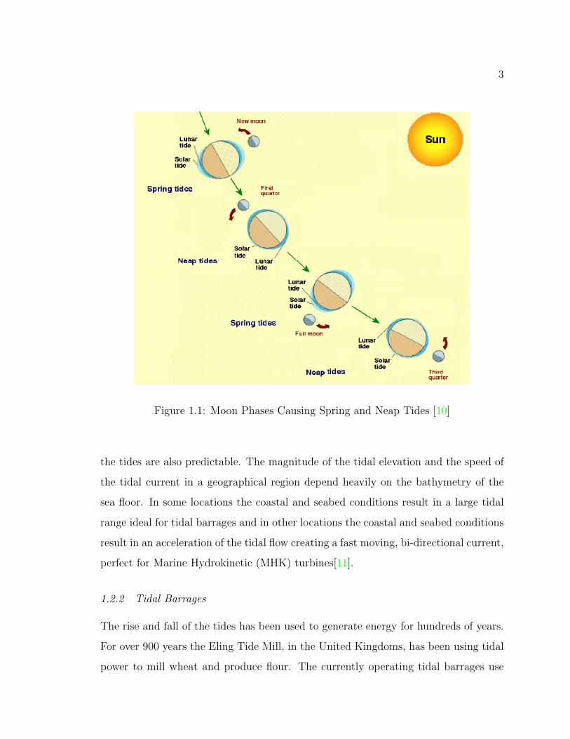
is greater than the average tidal range, see Figure 1.1 [9]. If the sun, moon, and
Earth create a right angle, the gravitational forces from the sun and the moon act
perpendicularly to each other, decreasing the magnitude of the tidal range such that
it is less than the average, this is called neap tide, see Figure 1.1.
Due to the predictability of celestial mechanics, the gravitational forces as well as
3
Figure 1.1: Moon Phases Causing Spring and Neap Tides [10]
the tides are also predictable. The magnitude of the tidal elevation and the speed of
the tidal current in a geographical region depend heavily on the bathymetry of the
sea floor. In some locations the coastal and seabed conditions result in a large tidal
range ideal for tidal barrages and in other locations the coastal and seabed conditions
result in an acceleration of the tidal flow creating a fast moving, bi-directional current,
perfect for Marine Hydrokinetic (MHK) turbines[11].
1.2.2 Tidal Barrages
The rise and fall of the tides has been used to generate energy for hundreds of years.
For over 900 years the Eling Tide Mill, in the United Kingdoms, has been using tidal
power to mill wheat and produce flour. The currently operating tidal barrages use

4
the same basic principle as the Eling Tide Mill. By storing water behind a dam at
high tide the tidal barrage creates a head difference as the water recedes to the low
tide level. The water stored behind the dam is then released through hydroelectric
turbines (a water wheel in the case of the flour mill) extracting energy from the
flowing water, see Figure 1.2 [10]. The largest energy-producing tidal barrage is a
240 MW tidal barrage in France, on the La Rance River estuary [10]. Currently
there are only three sites using tidal barrages due to the high capital cost and the
environmental impacts associated with this technology [8]. It has been suggested that
extracting energy from the kinetic energy of the flow instead of the tidal head loss
could potentially have significantly less environmental impact [12].
Figure 1.2: Tidal Barrage [7]
1.2.3 Marine Hydrokinetic Turbines
The principle behind MHK Turbines is to convert the kinetic energy in tidal currents
into mechanical energy by driving a generator to produce power [7]. There are two
primary types of MHK turbines, axial flow (also known as horizontal axis) turbines
and cross flow (also known as vertical axis) turbines, see Figure 1.3. The axis of
rotation for a horizontal axis turbine is parallel to the direction of the free stream
flow whereas the axis of rotation for a vertical axis turbine is perpendicular to the
direction of the free stream flow.

5
Figure 1.3: Horizontal Axis versus Vertical Axis Turbines [12]
The wind energy industry has determined through years of research that horizontal
axis turbines are the most effective mechanism for extracting energy from the wind at
large scale because the turbines can self-start and have a better efficiency than cross
flow turbines [12]. Many of the same theories and models developed for horizontal
axis wind turbines can be applied to modeling horizontal axis MHK turbines.
In the marine renewable energy industry there is no consensus on the leading tech-
nology for utility scale energy extraction. While the higher efficiency of horizontal
axis turbine still gives them an advantage, there are however, several problems faced
by horizontal axis turbines that present an opportunity for cross flow turbines to
compete in the MHK field:
• The high tip speed ratios required for high efficiency can cause cavitation to
occur
• Multiple turbines cannot share the same electrical converter [12]

6
• In order to extract the maximum amount of power from a bi-direction tidal flow
the turbine either needs to have symmetric blades, leading to lower efficiency,
or the turbine must be able to rotate about a vertical axis so that the turbine
is always aligned with the flow
Even though vertical axis turbines have been shown to be suboptimal for utility scale
wind turbines, the differences between wind and tidal currents make vertical axis
turbines a plausible option for the tidal energy field. In tidal currents, the flow will
always be perpendicular to the axis of rotation for vertical axis turbines allowing
them to operate with flow from any direction. Another benefit of using a vertical axis
turbine is they are well suited for use in turbine farms because they can be placed
relatively close to one another and if stacked vertically in a tower they only required
one generator [12]. There are several different blade designs for vertical axis turbines.
The two major designs are the classic Darrieus Turbine seen in Figure 1.3b and the
helical blade shaped turbine seen in Figure 1.4. The Darrieus Turbine suffers from
variable loading, whereas the helical shaped blades lead to an almost constant loading,
which can significantly extend the life of the turbine [12].
Figure 1.4: Helical blade shaped turbine [9]
7
1.2.4 Current Deployments
Some MHK turbines currently in use today are the Seagen, the Open-Centre Turbine,
the HS300, and the Turbine Generator Unit.
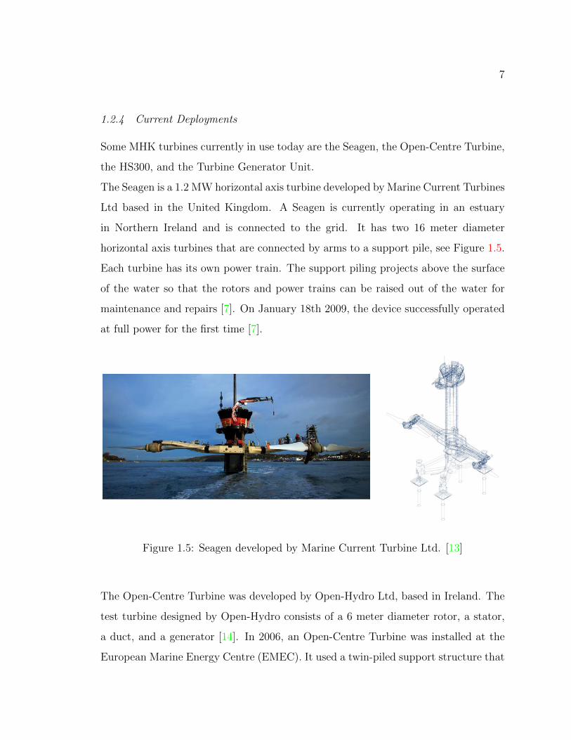
The Seagen is a 1.2 MW horizontal axis turbine developed by Marine Current Turbines
Ltd based in the United Kingdom. A Seagen is currently operating in an estuary
in Northern Ireland and is connected to the grid. It has two 16 meter diameter
horizontal axis turbines that are connected by arms to a support pile, see Figure 1.5.
Each turbine has its own power train. The support piling projects above the surface
of the water so that the rotors and power trains can be raised out of the water for
maintenance and repairs [7]. On January 18th 2009, the device successfully operated
at full power for the first time [7].
Figure 1.5: Seagen developed by Marine Current Turbine Ltd. [13]
The Open-Centre Turbine was developed by Open-Hydro Ltd, based in Ireland. The
test turbine designed by Open-Hydro consists of a 6 meter diameter rotor, a stator,
a duct, and a generator [14]. In 2006, an Open-Centre Turbine was installed at the
European Marine Energy Centre (EMEC). It used a twin-piled support structure that

8
allowed the turbine to be raised and lowered for testing purposes, see Figure 1.6a.
The commercial deployments of the turbine will be mounted to the seafloor and will
not have any surface penetration, see Figure 1.6b.
Figure 1.6: Open Centre Turbine developed by Open-Hydro Ltd. [15]
The HS300 was developed by Andritz Hydro Hammerfest, based in Norway. It is
a three bladed horizontal axis turbine. The HS300 is a 300kW prototype that has
been tested at a depth of 50 meters in Finnmark, Norway. The turbine successfully
completed a full cycle which included deployment, operation, retrieval, maintenance
and redeployment. The pre-commercial demonstrator, the HS1000, is a scaled up
version of the HS300 and is rated for 1 MW. It is currently deployed at the EMEC
tidal test site, where it has successfully provided power to the grid [16]. Andritz
Hydro Hammerfest is planning to install an array of turbines in the Sound of Islay,
see Figure 1.7
Ocean Renewable Power Company (ORPC) has developed the “Turbine Generator
Unit” (TGU). The TGU is a modular cross flow turbine, see Figure 1.8. These
cross flow turbines use the same principle as vertical axis turbines, where flow is
perpendicular to the axis of rotation. The axis of rotation for TGU’s, however, is
parallel to the seabed instead of vertical. The turbines are secured to the bottom

9
Figure 1.7: An artist’s rendition of the HS300 and HS1000 developed by Andritz
Hydro Hammerfest [16]
of the seafloor using a bottom support frame. In 2008, ORPC tested the TGU in
Cobscook Bay, Maine and it was a technical success. In 2010, they tested a pre-
commercial model of the TGU [17] and in 2012 installed the first commercial TideGen
system at the same location.
Figure 1.8: Tidal Generating Unit developed by Ocean Renewable Power Company
[17]

10
1.3 Wind Energy Versus Tidal Energy
In many ways, MHK turbines and wind turbines behave very similarly. Thus, many
of the same methods used to model wind turbines can be applied to MHK turbines.
Some of these methods, e.g. the Actuator Disc Model, the Blade Element Model, and
the Single Reference Frame model, are discussed in detail in Section 2.2. There are
several key differences between wind energy and tidal energy that must be taken into
consideration when modeling MHK turbines. One such difference, which is the focus
of this thesis, is the presence of a free surface because the fluid domain from which
MHK turbines extract energy is bounded by the interface between water and air.
1.3.1 Importance of the Free Surface
The free surface produces a significant difference between wind energy and tidal en-
ergy because the flow can no longer be assumed to be unconfined. The confinement
associated with the presence of the free surface and the sea floor introduces a new
parameter, the blockage ratio, that can increase the maximum power extracted from
the flow, relative to an unconfined turbine. The blockage ratio is defined as the swept
area of the turbine divided by the cross sectional area of the flow.
Besides the free surface’s direct effect on turbine performance through the blockage
ratio, the presence of the turbine also affects the free surface level, which can lead
to indirect effects on turbine performance and wake characteristics. The vertical
placement of a MHK turbine, which will affect free surface fluctuations, depends
greatly on the method used for installation. For example, a turbine supported by a
floating barge will most likely be close to the free surface whereas a turbine installed on
a gravity foundation will be close to the bottom of a channel [18]. Another factor used
in determining the vertical placement of a MHK turbine is the velocity gradient in
tidal channels. Turbines are believed to operate most efficiently near the free surface
because the maximum velocity typically occurs near the surface in tidal channels [19].

11
Adding a free surface into the numerical simulations of MHK turbines will complicate
the modeling and add computational cost. In some situations, the free surface fluctu-
ations may significantly affect the flow, in others it may be acceptable to ignore the
presence of the free surface because the effects are negligible. Thus, it is important
to determine when it is necessary to include the free surface in numerical modeling
of MHK turbines.
It is essential to understand the parameters that control flow around MHK turbines
in the presence of a free surface and to develop the non-dimensional parameters that
control the coupled turbine-free surface dynamics, in order to determine when it is
necessary to model the free surface since MHK turbines can have different diameters,
operate at different flow speeds, and at different depths. The non-dimensional number
typically applied to open channel flows is the Froude Number.
1.3.2 Froude Number
The Froude number is named after William Froude, a naval Architect who developed
the similarity concept for free surface flows [20]. The Froude number is typically
defined as
Fr =U√gl
(1.2)
where U is the flow speed, g is gravitational acceleration, and l is a characteristic
length scale. The depth of the water is most commonly used as the characteristic
length scale for open channel flows. The Froude number is a ratio of the speed of
the flow, U, to the speed of gravity waves,√gl. If the Froude number is small,
gravity waves propagate on the free surface both upstream and downstream. If, on
the other hand the Froude number is greater than one, then surface gravity waves
cannot propagate upstream against U (supercritical flow) and surface fluctuations
can only travel downstream (in a clear parallel with supersonic flow where pressure
12
waves cannot travel faster than the flow and therefore only propagate downstream).
For the flows studied in this thesis the Froude number is always much less than 1, as
discussed in Section 5.2.
The Froude number can be used to compare different flows in the same manner as
the Reynolds number. The Froude number allows free surface flows, with different
speeds and characteristic lengths, to be compared using a non-dimensional number in
order to characterize similarities in free surface behavior between different flows. The
challenge with applying the Froude number to flows with MHK turbines is defining
the right characteristic length scale. The most commonly used length scale is the
channel’s height (as is done in hydraulic engineering) which has been done by Myers
[21], Whelan [3], and Bahaj [22]. This length scale does not completely describe
the effects of a MHK turbine on the free surface profile. For example, a turbine
placed near the free surface in a very deep channel will interact differently with the
free surface than a turbine placed in the middle or bottom of that same channel.
Therefore, in this thesis, other possible length scales such as the distance from the
center of the turbine to the free surface, the distance from the tip of the turbine to
the free surface, and the turbine diameter will be examined.
1.4 Thesis Outline
Chapter 2, Literature Review, provides an overview of the current research available
for MHK turbines, specifically focusing on the operation of MHK turbines in confined
flows. Chapter 3, Methodology, describes the methodology and theory used in the
thesis. Chapter 4, Numerical Modeling, describes the generic numerical simulations
and model settings used in this thesis. Chapter 5, Results and Analysis, discusses
the results obtained through the numerical simulations. Chapter 6, Summary, Con-
clusions and Future Work, provides a summary of this thesis and highlights some of
the important conclusions.
13
Chapter 2
LITERATURE REVIEW
2.1 Energy Potential
It is essential to determine desirable site characteristics before considering the in-
stallation of MHK turbines in a given location. Most importantly, it needs to be
determined whether there is an amount of available kinetic energy in tidal flows at
those sites to make MHK turbines a viable energy source.
Every body of water is subject to the gravitational forces that result in the tides.
However, the amplitude of the tidal fluctuations and the magnitude of the tidal current
depend on the local bathymetry. In areas where the flow is spatially constrained like
between islands, around headlands, and estuarine-type inlets, there can be large tidal
variation and fast moving tidal currents resulting in high energy concentrations [23].
Many locations all around the world have been identified as containing suitable tidal
currents for power generation by MHK turbines. The important characteristics for
MHK turbine sites are fast moving tidal currents and a bi-directional flow. Frequently,
locations that meet both of these requirements have high levels of turbulent kinetic
energy. MHK turbines can suffer from rapid fatigue failure caused by the unsteady
loading resulting from high turbulence levels. Therefore, a detailed understanding
of the turbulent induced unsteady loading and a careful design process that takes
this engineering challenge into account is critical for the success of MHK turbines
in the harsh environment associated with the best resource sites. The restriction of
maintenance in an underwater environment may make the robustness of the design
even more critical for MHK turbines than it is already in wind turbines.
It is also important to determine the maximum power that can be extracted from
14
the flow. For wind energy, which deals with an unconstrained incompressible flow,
the maximum coefficient of power is equal to 0.593 [24] [25]. This is known as Betz
limit and was derived using a stream-tube analysis of the flow around a turbine. The
coefficient of power is defined as
Cp =Power12ρU3∞Ad
(2.1)
where Power is the power generated by the turbine, ρ is the density of the fluid,
U∞ is the free stream velocity, and Ad is the area of the turbine. This approach is
commonly referred to as the Linear Momentum Theory - Actuator Disc Model [25].
The derivation of the Actuator Disc Model is described in detail in Section 3.3.
For tidal energy, even though the current flow speed is typically slower than in wind,
the relatively high density of water results in an energy density of tidal currents
that makes it recoverable within engineering and economic parameters under certain
conditions [23]. Therefore, in locations where currents are bi-directional and velocities
exceed 2 m/s, a sufficient amount of energy can be extracted to make tidal energy a
viable method of power generation.
In unconstrained flows, or flows with a very small blockage ratio, a MHK turbine will
behave similarly to a wind turbine and the Betz Limit can still be applied. However,
in many cases, the bathymetry of the potential tidal energy sites and the presence of
the free surface constrain the flow and the Betz Limit no longer applies [1], making
power coefficients above 59% or even above 100% possible. Several different methods
have been derived to determine the available power and maximum coefficient of power
in such cases. According to Garrett [1]:
Pmax =16
27(1− ε)−21
2ρAdU
3∞ (2.2)
where ε is the blockage ratio, which is defined as the area of the turbine (Ad) divided
by the cross sectional area of the flow, ρ is the fluid density, and U∞ is the free stream

15
velocity. There is an extra efficiency multiplier of (1 − ε)−2 resulting from the flow
being constrained. This extra efficiency term goes to one as the blockage ratio goes
to zero, reproducing Betz limit.
Garrett′s analysis above, [1], only accounted for the increased blockage ratio because
it represents a one-dimensional analysis between two rigid surfaces. The analysis did
not address the issue of a change in free surface height resulting from the energy
extracted by the MHK turbine potentially affecting the overall energy budget.
Whelan [3] used a similar analysis but accounted for both the blockage ratio and the
change in free surface height due to the pressure drop across the turbine related to
the energy extracted by the turbine. The extraction of energy (potential and kinetic)
is related to the change in pressure as follows:
Pext = Ut ·∆P · Ad (2.3)
where ∆P is the change in pressure across the turbine and Ut is the velocity at the
turbine. This analysis, [3], uses conservation of mass, conservation of momentum in
the stream wise direction, and conservation of energy to develop the theory. The
derivation provides an equation for the coefficient of power that is a function of the
Froude Number, the blockage ratio, and the axial induction factor. The expression
for the axial induction factor is given in Equation 3.31. Given those same values, the
change in height of the free surface non-dimensionalized by the initial channel height
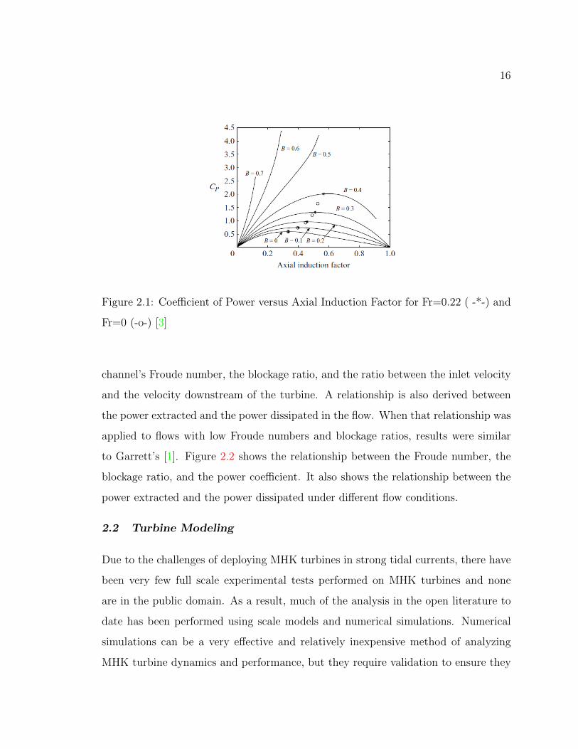
can also be calculated. Figure 2.1 shows the coefficient of power (Cp) for a given value
of the channel’s Froude Number (Fr = 0.22) at different axial induction factors and
blockage ratios. It should be noted that a high blockage ratio can lead to a decrease
in the free stream velocity subsequently lowering the maximum power available but
not the coefficient of power.
In Whelan et al.’s results, the control volume used did not include the region where
wake mixing occurs. Polagye [26] performed a similar analysis but included the mixing
region. In this analysis, like in Whelan et al.’s, the power extracted depends on the
16
Figure 2.1: Coefficient of Power versus Axial Induction Factor for Fr=0.22 ( -*-) and
Fr=0 (-o-) [3]
channel’s Froude number, the blockage ratio, and the ratio between the inlet velocity
and the velocity downstream of the turbine. A relationship is also derived between
the power extracted and the power dissipated in the flow. When that relationship was
applied to flows with low Froude numbers and blockage ratios, results were similar
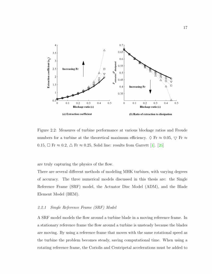
to Garrett’s [1]. Figure 2.2 shows the relationship between the Froude number, the
blockage ratio, and the power coefficient. It also shows the relationship between the
power extracted and the power dissipated under different flow conditions.
2.2 Turbine Modeling
Due to the challenges of deploying MHK turbines in strong tidal currents, there have
been very few full scale experimental tests performed on MHK turbines and none
are in the public domain. As a result, much of the analysis in the open literature to
date has been performed using scale models and numerical simulations. Numerical
simulations can be a very effective and relatively inexpensive method of analyzing
MHK turbine dynamics and performance, but they require validation to ensure they
17
Figure 2.2: Measures of turbine performance at various blockage ratios and Froude
numbers for a turbine at the theoretical maximum efficiency. ♦ Fr ≈ 0.05, 5 Fr ≈
0.15, � Fr ≈ 0.2, 4 Fr ≈ 0.25, Solid line: results from Garrett [1]. [26]
are truly capturing the physics of the flow.
There are several different methods of modeling MHK turbines, with varying degrees
of accuracy. The three numerical models discussed in this thesis are: the Single
Reference Frame (SRF) model, the Actuator Disc Model (ADM), and the Blade
Element Model (BEM).
2.2.1 Single Reference Frame (SRF) Model
A SRF model models the flow around a turbine blade in a moving reference frame. In
a stationary reference frame the flow around a turbine is unsteady because the blades
are moving. By using a reference frame that moves with the same rotational speed as
the turbine the problem becomes steady, saving computational time. When using a
rotating reference frame, the Coriolis and Centripetal accelerations must be added to

18
the momentum equation [27]. The SRF model is capable of capturing the boundary
layer that develops along the surface of the blade, as well as flow separation, requiring
a very fine mesh near the blade. This results in a relatively large computational grid
and long computational runtimes. For example, when modeling the NREL phase VI
turbine, the ADM and BEM only required 1.65 million mesh elements, whereas, the
SRF model required 5.1 million mesh elements and it took about 24 times longer to
converge [27]. For that reason, it can be beneficial to use a simpler model that does
not include the blade geometry.
2.2.2 Actuator Disc Model (ADM)
ADM is based on one dimensional stream tube analysis of the flow. In this analysis
the turbine is represented by a body force that is applied to the flow, see Figure 2.3
[25]. The force is applied uniformly over the swept area of the turbine. The derivation
of the ADM is provided in Section 3.3. In numerical simulations and lab experiments,
the turbine is represented by a porous media in the shape of a disc, referred to as an
actuator disc, which applies a force to the flow similar to the thrust force of a turbine
[28].
An actuator disc causes a constant resistance to a flow field that imposes the thrust
force on the flow [29]. The magnitude of force is a function of the resistant coefficient
of the porous media and the incoming flow speed. The porosity of the disc can be
changed in order to change the resistant coefficient and subsequently the thrust force
[29]. It should be noted that different materials (or materials with different pore sizes)
even with the same porosity can produce different thrusts and different wake deficits
due to the flow characteristics through the pores [23].
The ADM is a simplistic model that has relatively short computational times when
compared to the BEM and the SRF model [27]. The shorter computational time is
partially due to the fact that the flow can be considered steady-state because the
turbine is modeled as a disc instead of rotating blades [29]. The short time is also a

19
Figure 2.3: Energy Extracting Stream-Tube of a Wind Turbine [25]
result of the mesh resolution. The boundary layer and flow separation on the blades
are not being modeled. Furthermore, because of the disc’s simplicity, some of the
flow physics are not captured. For example, porous discs used experimentally do not
extract energy, but instead the disc turns kinetic energy into small scale turbulence
that dissipates quickly. Vortex shedding is also different for a porous disc than for a
turbine, and the disc does not induce any swirl [28].
In numerical simulations, the actuator disc is implemented by creating a zone in the
fluid domain with the same cross sectional area as the turbine rotor and defining it
as a porous zone. The porous zone is represented by a source term in the momentum
equation [30].
2.2.3 Blade Element Model (BEM)
The ADM has been shown to not accurately model the near wake behavior of a MHK
turbine and has been shown to under predict the velocity deficit in the far wake [27].
Thus, it may be beneficial to use a model that captures more of the physics of the
turbine. Two such models that have been applied to MHK turbines as well as wind
turbines are: the Blade Element Model (BEM) and the Blade Element Momentum
Theory (BEMT) Model. BEM applies Blade Element Theory (BET) and the BEMT
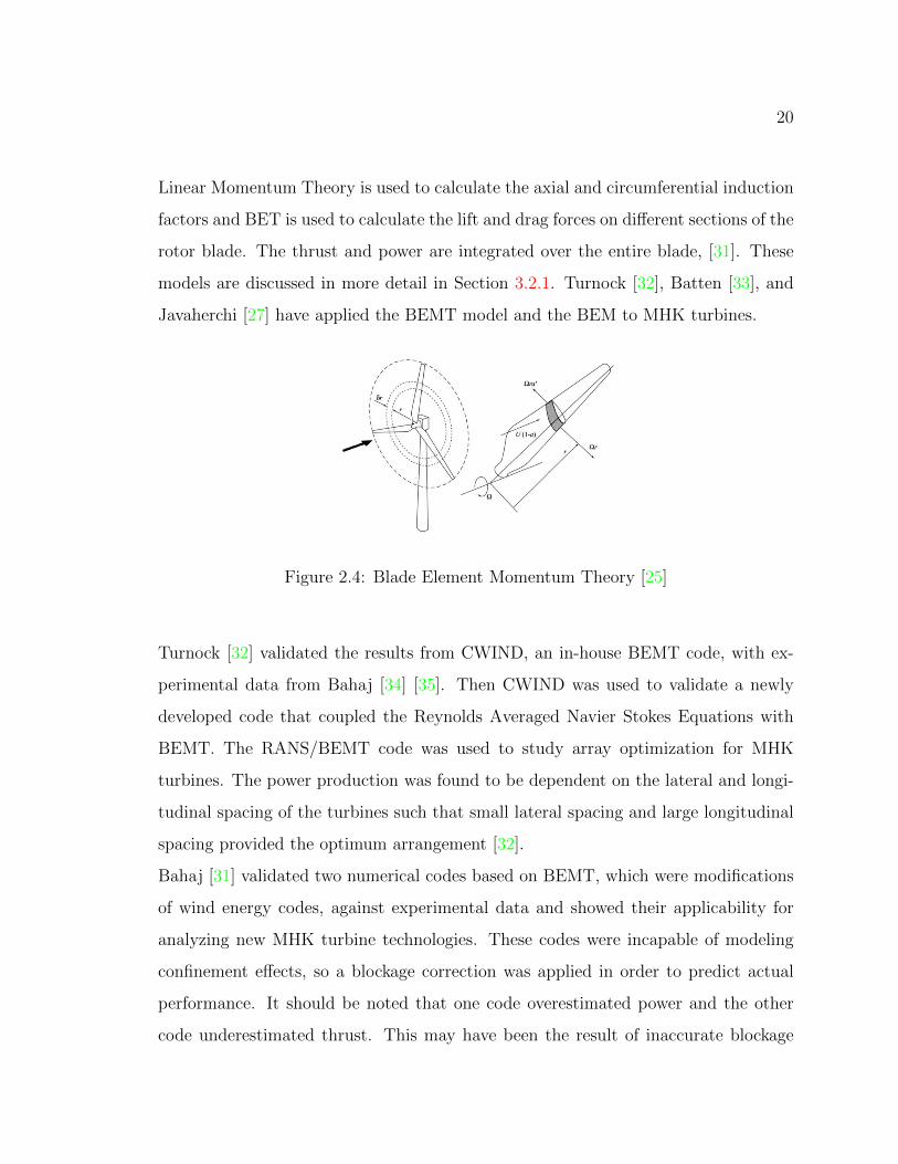
model combines BET with Linear Momentum Theory (LMT), see Figure 4.5 [31].
20
Linear Momentum Theory is used to calculate the axial and circumferential induction
factors and BET is used to calculate the lift and drag forces on different sections of the
rotor blade. The thrust and power are integrated over the entire blade, [31]. These
models are discussed in more detail in Section 3.2.1. Turnock [32], Batten [33], and
Javaherchi [27] have applied the BEMT model and the BEM to MHK turbines.
Figure 2.4: Blade Element Momentum Theory [25]
Turnock [32] validated the results from CWIND, an in-house BEMT code, with ex-
perimental data from Bahaj [34] [35]. Then CWIND was used to validate a newly
developed code that coupled the Reynolds Averaged Navier Stokes Equations with
BEMT. The RANS/BEMT code was used to study array optimization for MHK
turbines. The power production was found to be dependent on the lateral and longi-
tudinal spacing of the turbines such that small lateral spacing and large longitudinal
spacing provided the optimum arrangement [32].
Bahaj [31] validated two numerical codes based on BEMT, which were modifications
of wind energy codes, against experimental data and showed their applicability for
analyzing new MHK turbine technologies. These codes were incapable of modeling
confinement effects, so a blockage correction was applied in order to predict actual
performance. It should be noted that one code overestimated power and the other
code underestimated thrust. This may have been the result of inaccurate blockage

21
corrections. The lift and drag coefficients required for the blade element models were
determined using Xfoil, a 2-D potential flow airfoil performance code.
Javaherchi [27] performed numerical simulations using the SRF model, the Actuator
Disc Model, and an implementation of the BEM, the Virtual Blade Model (VBM).
The NREL Phase VI wind turbine was first simulated using the three different models.
The results from these simulations were validated against public results. Once the
simulation models were partially validated on HAWT experimental results, the same
methodology was applied to MHK turbines. He showed that VBM, when applied to
MHK turbines, was generally in good agreement with the more accurate SRF model.
Some of the differences between the two models were: the VBM did not resolve all of
the details directly downstream of the turbine, and the tip vortices were not properly
captured. The SRF model showed that the wake became axi-symmetric a short
distance downstream of the turbine (1-2 D). This would enable a simpler model to
be applied for studies only requiring information on the far wake. Javaherchi showed
that ADM failed to capture the flow physics directly behind the turbine as well as
any tip vortex shedding. In addition, it was shown that the velocity deficit for the
ADM in the near wake was significantly different than the wake deficit of the SRF
model and the VBM [27]. Javaherchi concluded the VBM was the best choice to use
in future studies of the behavior of the far wake.
2.3 Free Surface Effects on MHK Turbines
In many ways, tidal energy is similar to wind energy and the same modeling techniques
can be applied to both. However, there are several key differences. Wind turbines
convert kinetic energy off the bottom of the atmospheric boundary layer and, since
wind turbines only take a very small portion of the total energy and the pressure
wake recovers, the flow can be treated as unconstrained [19]. Tidal energy, on the
other hand, converts potential energy into usable power. Decreasing the potential
energy in the channel lowers the channel depth at the outlet, which causes the flow to

22
accelerate in order to conserve mass, hence for tidal energy, the kinetic energy in the
flow is increased. In some regions where MHK turbines can potentially be installed,
the depth of the turbine is on the same scale as the turbine diameter which can affect
the power produced. The wake structure may be influenced by the proximity of the
turbine to the free surface or sea floor because the presence of a boundary can lead
to flow acceleration above and below the turbine [23].
According to Myers [23], the upper 15 meters of a waterway experience the effects of
wave generated turbulence, and the bottom one-third of the waterway has high levels
of turbulent fluctuations, resulting from the influence of the bottom boundary layer.
This makes the middle third of the water column the most suitable for MHK turbine
installations, see Figure 2.5. Many waterways such as rivers or estuaries where MHK
turbines maybe placed, however, are not deep enough to avoid the upper 15 meters
of the water column. Therefore, the turbine may experience the effects of the free
surface presence.
Figure 2.5: Some factors that affect turbine performance and wake structure [22]
2.3.1 Experiments Conducted with a Free Surface
Producing a small scale model of a horizontal axis turbine is very difficult because it
is impossible to maintain all of the important non-dimensional numbers, such as the

23
Reynolds number, Tip Speed Ratio, Coefficient of Thrust, Coefficient of Power, and
some form of the Froude number, without significantly changing the downstream flow
[23]. Therefore, it is sometimes necessary to use an alternative method for modeling
a turbine. Myers [23], used a porous disc as a reasonable substitute for an actual
turbine because the structure of the near wake has a small effect on the far wake
properties. The porous disc creates a thrust which can be adjusted by changing the
porosity of the disc, and the area of the disc can be the same as the swept area of the
turbine. These factors help to maintain some flow properties.
Scaling of open channel flow itself involves maintaining two important non-dimensional
numbers, the Reynolds number and the Froude number. Scaling of both of these
numbers experimentally is not possible. For bounded flows, the Froude number is
important because of the close proximity of the free surface where the gravitational
effects cannot be ignored [23], and the Reynolds number is important because of the
proximity of the seabed where viscous forces cannot be ignored [21]. Most experi-
ments maintain Froude number similarity while ensuring the experiments’ Reynolds
number is in the same turbulent regime as the full-scale turbine [21].
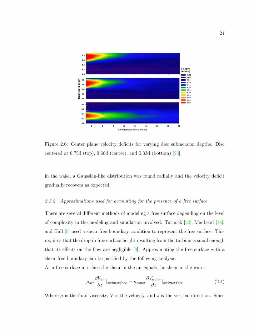
Myers [21] performed several experiments where the vertical position of a porous disc
was varied to determine how the vertical position affects the turbine wake. In the
experiments, the disc was centered at 0.33d, 0.5d, 0.66d, and 0.75d where d is the
depth of the channel. The turbine’s diameter was 0.25d. When the disc was centered
at 0.66d and 0.75d it produced very similar velocity deficits to the disc at 0.5d [21],
see Figure 2.6. By examining the wake, it can be seen that with a constrained flow
the axi-symmetric wake assumption, which is sometime applied for wind turbines, is
no longer valid [23]. Myers did not comment on the free surface fluctuations.
Sun [19] also performed experiments involving a free surface. A mesh disc was used
to represent the turbine, considering the thrust force as the main factor in wake
development [19]. The experiment was performed in the field instead of a flume to
simulate realistic operating conditions. According to the velocity profiles measured
24
Figure 2.6: Center plane velocity deficits for varying disc submersion depths. Disc
centered at 0.75d (top), 0.66d (center), and 0.33d (bottom) [23].
in the wake, a Gaussian-like distribution was found radially and the velocity deficit
gradually recovers as expected.
2.3.2 Approximations used for accounting for the presence of a free surface
There are several different methods of modeling a free surface depending on the level
of complexity in the modeling and simulation involved. Turnock [32], MacLeod [36],
and Hall [9] used a shear free boundary condition to represent the free surface. This
requires that the drop in free surface height resulting from the turbine is small enough
that its effects on the flow are negligible [9]. Approximating the free surface with a
shear free boundary can be justified by the following analysis.
At a free surface interface the shear in the air equals the shear in the water.
µair∂Vair∂z|z=interface = µwater
∂Vwater∂z
|z=interface (2.4)
Where µ is the fluid viscosity, V is the velocity, and z is the vertical direction. Since

25
the µair � µwater
µairµwater
∂Vair∂z|z=interface =
∂Vwater∂z
|z=interface ≈ 0 (2.5)
Implying, the shear is approximately zero and the boundary can be assumed to be
shear free but this does not account for any surface fluctuations that may occur.
Myers’ numerical model [21] took a different approach. The vertical and horizontal
wake expansions were decoupled so the vertical wake expansion could have boundaries
applied. Then, the two separate wakes were solved and their solutions combined
to obtain the full wake. The shear-layer Navier Stokes equation for axi-symmetric
flows and an eddy-viscosity turbulence model, requiring a length scale and a velocity
scale, were used to calculate the Reynolds Stresses. The wake width was used as
the length scale and the centerline velocity deficit was used as the velocity scale
[21]. The wake width and centerline velocity deficit were derived from semi-empirical
equations in order to provide a Gaussian velocity profile [21]. When the solution
was decoupled, the horizontal wake portion could be treated as axi-symmetric and
unconstrained. The vertical portion of the wake had to be treated differently because
of the effects of the bounding surfaces. To account for the limited expansion caused
by the bounding surfaces, the vertical wake width was restricted [21]. This approach
allowed the axi-symmetric assumption to be used on the vertical wake minimizing
computational expenses. The upper and lower regions of the vertical wake could
also behave differently depending on the proximity to the bounding surfaces, thus,
the model could be further decoupled to separate the upper and lower vertical shear
layers. The individual shear layers were first solved separately, before combining
their solutions to obtain the solution for the full wake [21]. The results provided
good agreement with experimental data, but there were some discrepancies near the
bounding surfaces.
26
2.3.3 Modeling the Free Surface
Harrison [29], Sun [19][18], and Consul [37] studied the effect of simulating free surface
fluctuations in the computational modeling of MHK turbines. According to Harrison,
modeling the free surface is the most suitable option to capture the possible flow
deceleration near the surface of an open channel resulting from secondary currents
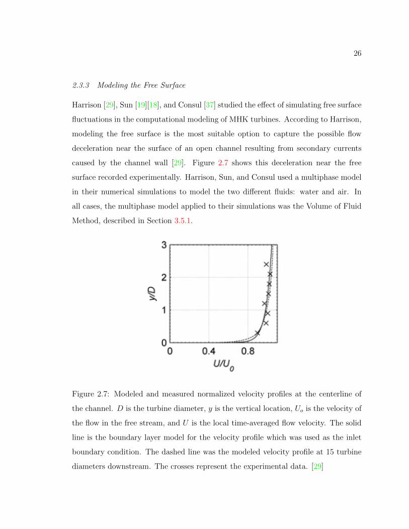
caused by the channel wall [29]. Figure 2.7 shows this deceleration near the free
surface recorded experimentally. Harrison, Sun, and Consul used a multiphase model
in their numerical simulations to model the two different fluids: water and air. In
all cases, the multiphase model applied to their simulations was the Volume of Fluid
Method, described in Section 3.5.1.
Figure 2.7: Modeled and measured normalized velocity profiles at the centerline of
the channel. D is the turbine diameter, y is the vertical location, Uo is the velocity of
the flow in the free stream, and U is the local time-averaged flow velocity. The solid
line is the boundary layer model for the velocity profile which was used as the inlet
boundary condition. The dashed line was the modeled velocity profile at 15 turbine
diameters downstream. The crosses represent the experimental data. [29]
27
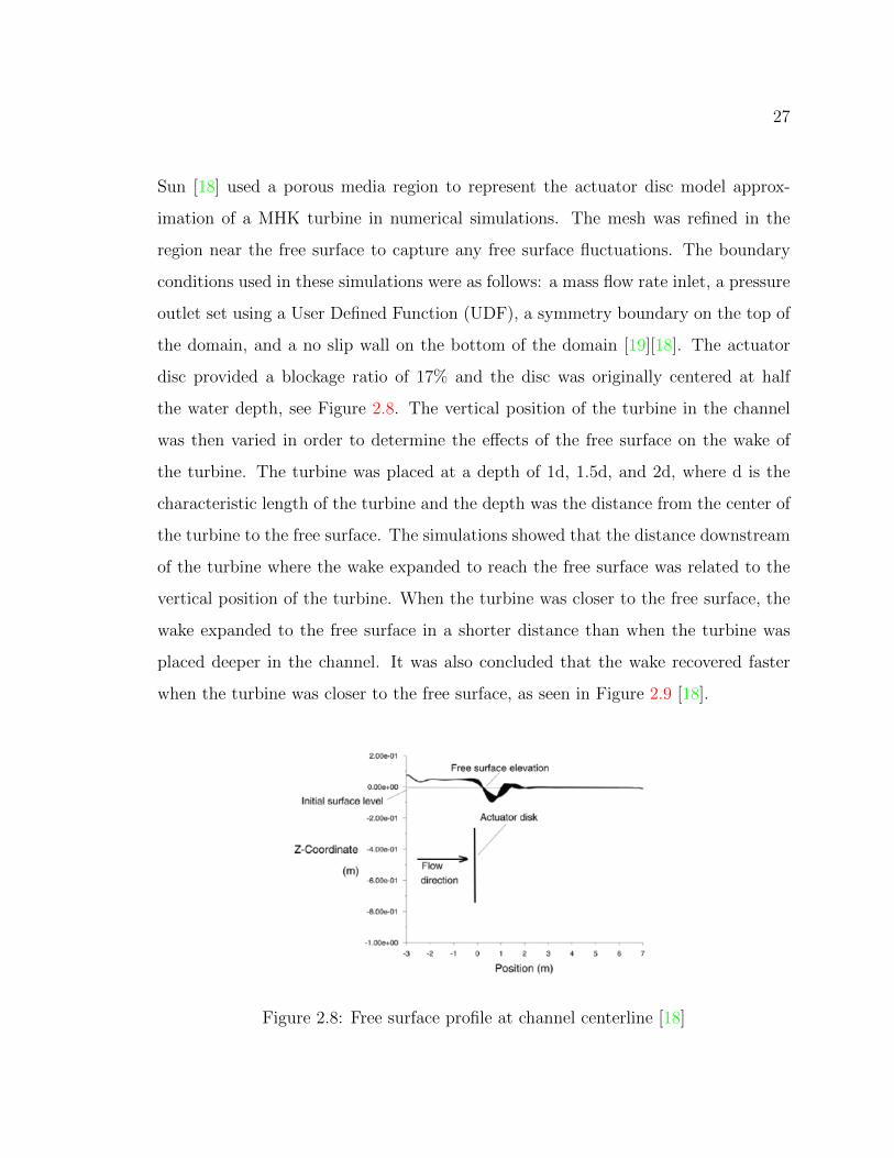
Sun [18] used a porous media region to represent the actuator disc model approx-
imation of a MHK turbine in numerical simulations. The mesh was refined in the
region near the free surface to capture any free surface fluctuations. The boundary
conditions used in these simulations were as follows: a mass flow rate inlet, a pressure
outlet set using a User Defined Function (UDF), a symmetry boundary on the top of
the domain, and a no slip wall on the bottom of the domain [19][18]. The actuator
disc provided a blockage ratio of 17% and the disc was originally centered at half
the water depth, see Figure 2.8. The vertical position of the turbine in the channel
was then varied in order to determine the effects of the free surface on the wake of
the turbine. The turbine was placed at a depth of 1d, 1.5d, and 2d, where d is the
characteristic length of the turbine and the depth was the distance from the center of
the turbine to the free surface. The simulations showed that the distance downstream
of the turbine where the wake expanded to reach the free surface was related to the
vertical position of the turbine. When the turbine was closer to the free surface, the
wake expanded to the free surface in a shorter distance than when the turbine was
placed deeper in the channel. It was also concluded that the wake recovered faster
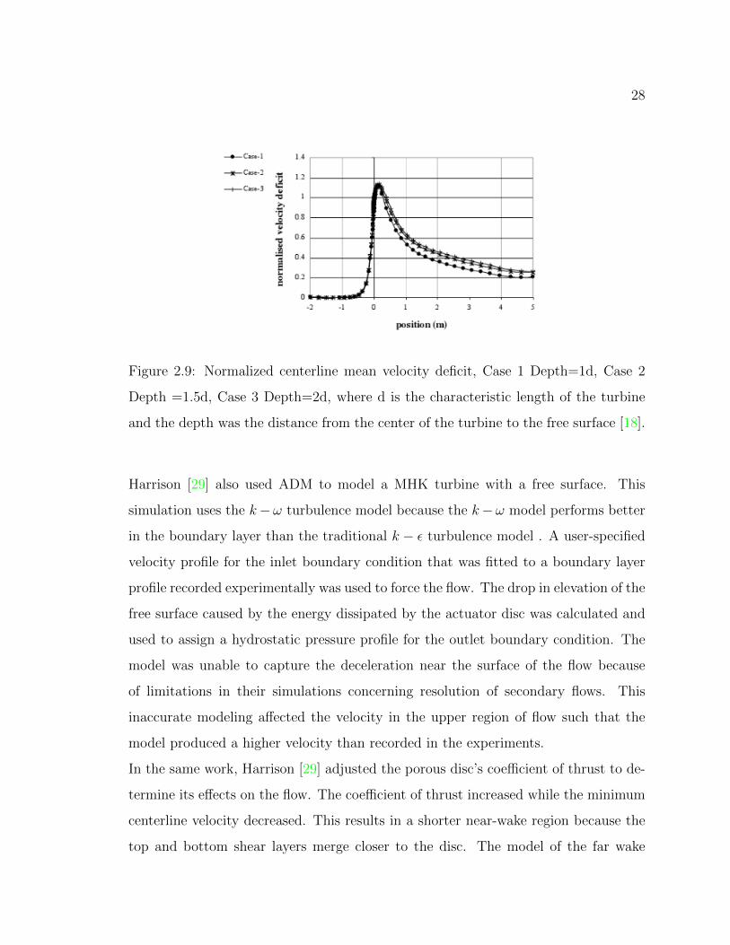
when the turbine was closer to the free surface, as seen in Figure 2.9 [18].
Figure 2.8: Free surface profile at channel centerline [18]
28
Figure 2.9: Normalized centerline mean velocity deficit, Case 1 Depth=1d, Case 2
Depth =1.5d, Case 3 Depth=2d, where d is the characteristic length of the turbine
and the depth was the distance from the center of the turbine to the free surface [18].
Harrison [29] also used ADM to model a MHK turbine with a free surface. This
simulation uses the k−ω turbulence model because the k−ω model performs better
in the boundary layer than the traditional k − ε turbulence model . A user-specified
velocity profile for the inlet boundary condition that was fitted to a boundary layer
profile recorded experimentally was used to force the flow. The drop in elevation of the
free surface caused by the energy dissipated by the actuator disc was calculated and
used to assign a hydrostatic pressure profile for the outlet boundary condition. The
model was unable to capture the deceleration near the surface of the flow because
of limitations in their simulations concerning resolution of secondary flows. This
inaccurate modeling affected the velocity in the upper region of flow such that the
model produced a higher velocity than recorded in the experiments.
In the same work, Harrison [29] adjusted the porous disc’s coefficient of thrust to de-
termine its effects on the flow. The coefficient of thrust increased while the minimum
centerline velocity decreased. This results in a shorter near-wake region because the
top and bottom shear layers merge closer to the disc. The model of the far wake

29
accurately predicted the trends of the experimental data. The level of agreement,
however, varied with the vertical location of the actuator disc. The model deviated
increasingly from the experimental data when it was closer to the free surface.
Consul [37] modeled a cross flow turbine in an open channel. He performed two dif-
ferent sets of simulations. One set used a shear free boundary to represent the free
surface, referred to as rigid lid simulation. The other set of simulations allowed for de-
formation of the free surface by applying the Volume of Fluid multiphase model. The
turbine used for the simulations was a three bladed Darrieus turbine. The simulations
were performed in a two-dimensional plane perpendicular to the axis of rotation. The
geometry of the blade’s airfoil was modeled to resolve the flow past the blades, and
the blades were rotated using a sliding mesh. Three different blockage ratios were
examined, 50%, 25%, and 12.5%. Consul observed that the coefficient of power (Cp)
increased with an increase in blockage ratio, and the Tip Speed Ratio (λ) that corre-
sponds to the maximum Cp increased with the increase in blockage ratio, see Figure
2.10.
Consul also examined the effects of the shear free boundary approximation on the
flow. He concluded that at low blockage ratios the Cp was approximately the same
for both the rigid lid simulations and the VOF simulations. At high blockage ratios,
e.g. 50%, however, the Cp for the VOF simulation was 6.7% greater than the rigid
lid simulation [37]. The influence of the Froude number on the performance of the
turbine was also discussed. The length scale used for the Froude number was the
channel depth. For simulations with a blockage ratio of 50% the Cp depended on
the upstream Froude number, matching the prediction of Whelan [3], see Figure 2.11.
The change in height of the free surface also varied with the upstream Froude number.
This issue of choice of non-dimensional parameters will be discussed in Section 5.2 of
this thesis.

30
Figure 2.10: Dependency of turbine power coefficient, Cp, on blockage and free-surface
model (RL, rigid lid; VOF, volume of fluid) [37].
2.4 Motivation for the Work Performed in this Thesis
There has been a limited amount of research studying the effects of a free surface
on the operating characteristics of MHK turbines. The studies discussed previously,
with the exception of Consul’s paper [37] which focused on a two-dimensional analysis
of a cross flow turbine, focused on the effect of the confining surfaces on the wake
characteristics. These studies do not address the power extracted by the turbine or
the free surface fluctuations that result from the turbine. Those are the primary issues
addressed in this thesis.
In most potential MHK turbine locations, the blockage ratio will be low enough,
and the free surface distance to the turbine will be large enough, that the presence
of a free surface will not affect the turbine performance or the fluctuations in free

31
Figure 2.11: Power coefficient, Cp, for various Fr, for a flow with a blockage ratio of
50% [37].
surface height. However, there are a number of key issues that make the study of
effects of the blockage ratio and the turbine depth on the operating characteristics
of MHK turbines relevant. As discussed previously, performing full scale testing of
MHK turbines is very challenging, so significant research work has been performed
using scale models in flumes. In flume experiments, the blockage ratio is typically
much higher, and the free surface much closer to the turbine rotor, than what will
be seen in the field. Thus, it is important to determine if the coefficient of power
found experimentally has been affected by the unnaturally high blockage ratio or free
surface effects. Furthermore, there are some bodies of water, such as rivers, channels,
and estuaries, where the blockage ratio can potentially be high enough, or the free
surface distance to the turbine low enough, to affect the flow. In this situations, it is
important to determine the limiting values for the parameters that control free surface

32
effects so that the MHK turbine installation can avoid or plan for those influences in
a quantitative manner.

33
Chapter 3
METHODOLOGY
3.1 Numerical Modeling Theory
The non-linearity and turbulent nature of fluid flows of interest in Marine Hydroki-
netic Energy prevent all but the simplest of these fluid mechanics problems from
having closed form solutions. A powerful alternative, along with experimentation, is
to solved them numerically. Computational Fluid Dynamics (CFD) has become, over
the last four decades, a significant source of physical understanding and engineer-
ing modeling to complement mathematical exact solutions and laboratory and field
experiments.
The CFD software used for this thesis is ANSYS Fluent, version 14.0. Fluent is
a Finite Volume Solver. The numerical algorithm used in a Finite Volume Solver
“consists of the following steps:
• Integration of the governing equations of fluid flow over all the (finite) control
volumes of the domain.
• Discretization - conversion of the resulting integral equations into a system of
algebraic equations.
• Solution of the algebraic equations by an iterative method.” [38]
3.1.1 Governing Equations
The problem domain is broken up into smaller volumes called elements. Fluent ap-
plies user specified boundary conditions and initial conditions to the domain in order

34
to solve the governing equations for the mean flow variables in each fluid element.
The governing flow equations used are the Reynolds Averaged Navier Stokes (RANS)
equations. The RANS equations are derived by substituting the Reynolds Decom-
position for turbulent fluid variables, velocity and pressure for incompressible flows,
into the conservation of mass and momentum equations, then time-averaging the
equations. The Reynolds Decomposition of the velocity and pressure expresses the
instantaneous values of those variables and their derivatives as the sum of a mean,
“expected”, value and the fluctuating value:
ui = ui + u′i (3.1)
p = p+ p′ (3.2)
where u is the mean flow velocity, p is the mean pressure, u′ is the fluctuating velocity,
and p′ is the fluctuating pressure. The resulting RANS equations, written in tensor
notation, are laid out in Equations 3.3 and 3.4:
∂ρ
∂t+
∂
∂xi(ρui) = 0 (3.3)
∂
∂t(ρui) +
∂
∂xi(ρuiuj) = − ∂p
∂xi+
∂
∂xj
[µ
(∂ui∂xj
+∂uj∂xi
)]+
∂
∂xj(−ρu′iu′j) + Si (3.4)
The RANS equations contain many of the same terms found in the instantaneous con-
servation of mass and momentum equations, such as a temporal acceleration term,
the convective acceleration term, a pressure gradient term, the viscous stress gradi-
ent term, and a source term, Si [38]. The RANS equations are formulated with the
mean velocity and mean pressure as the key unknowns, instead of the instantaneous
velocity and instantaneous pressure in the Navier Stokes equation. The RANS equa-
tions, however, have an additional term containing the fluctuating velocities. This
additional term, −ρu′iu′j, is traditionally referred to as the Reynolds Stress term, and
it represents the effects of turbulence transport on the mean flow. This term, which

35
potentially represent nine independent unknowns separate from the mean velocity
components and pressure must be expressed in terms of those key variables, in order
to make the RANS equations a mathematically sound problem (four equations and
four unknowns). This important aspect of the RANS equations and their methods of
solution for turbulent flows is classically referred to as the closure problem.
3.1.2 Turbulence Modeling
The closure problem described in the previous paragraph presents a requirement to
model the Reynolds stresses as a function of other resolved variables in the problem.
This has given rise to a wide variety of turbulence modeling approaches, compatible
with the basic premise of the RANS equation, to close the problem in a manage-
able systems of equations that can be solved computationally. One commonly used
approach is the Boussinesq Hypothesis, which states that the Reynolds stresses are
proportional to the mean shear in the flow (and have zero trace to be compatible with
the incompressibility condition):
−ρu′iu′j = µt
(∂ui∂xj
+∂uj∂xi
)− 2
3ρkδij (3.5)
where k is the turbulent kinetic energy, µt is the turbulent viscosity, and δij is the
Dirac Delta, from [38]. Through dimensional analysis, it can be shown that the
turbulence viscosity term could be written as:
µt = Cρvl (3.6)
where C is a coefficient, ρ is the density, v is a velocity scale, and l is a length scale
[38]. Many different models have been developed to solve for the turbulent viscosity
by defining different length and velocity scales. The models all have varying degrees
of accuracy. For the most part, the more accurate the model, the longer the CFD
simulation takes to reach a solution. The method used in this thesis is called the
36
k − ε turbulence model. The k − ε model was chosen because it is a commonly used,
robust turbulence model. Since the model used to represent the turbine’s effects on
the flow does not have a solid boundary and the effects of the channel bottom are
not of primary importance to the research performed here, the mesh in that region
was not refined in a way to resolve the boundary layer, so a turbulence model like the
k − ω turbulence model or Spalart-Allmaras turbulence model, that more accurately
models flow near a solid surface, were not required. The length scale and velocity
scale for the k − ε model are
v = k1/2 (3.7)
l =k3/2
ε(3.8)
where k is the turbulent kinetic energy and ε is the turbulent dissipation rate. Such
that
µt = ρCµk2
ε(3.9)
where Cµ is a dimensionless constant normally taken to be Cµ = 0.09. Thus, k and ε
must be calculated to obtain the turbulent viscosity. The turbulent kinetic energy is
equal to
k =1
2u′i
2 (3.10)
and the turbulent dissipation rate is equal to
ε = 2ν(s′ij · s′ij) (3.11)
s′ij =1
2
(∂u′i∂xj
+∂u′j∂xi
)(3.12)

37
k and ε depend on the fluctuating part of the velocity and their respective trans-
port equations depend on fluctuating velocity and pressure terms. Therefore, neither
equation can be solved for directly with only the mean flow terms. In order to solve
for k and ε, the fluctuating terms in their transport equations must be modeled using
mean flow quantities and coefficients. This is done for the turbulent kinetic energy
transport equation by dividing the terms into a temporal rate of change term, a con-
vection term, a diffusion term, a production term based on the mean shear and a
destruction term based on the turbulent dissipation rate, [38]
∂(ρk)
∂t+
∂
∂xi(ρkui) =
∂
∂xi
(µtσk
∂k
∂xi
)+ 2µtSij · Sij − ρε (3.13)
where σk is the turbulent Prandtl number for kinetic energy, typically taken to be
σk = 1, and Sij is the mean strain rate
Sij =1
2
(∂ui∂xj
+∂uj∂xi
). (3.14)
The equation for the turbulent dissipation rate used as part of the k − ε model is
purely empirical. ε is commonly viewed as the rate of energy transfer from large
scales to small scales through the turbulent cascade. As such it can be determined
entirely by the large and inertial scale motions, and not the dissipative range. The
exact equation for ε would contains multiple dissipative range processes but that
would un-necessarily complicate the calculation, therefore the equation for ε used in
the k − ε model is based on larger scale motion and as a result is empirical. It has
a similar structure to the turbulent kinetic energy transport equation: a temporal
rate of change term, a convection term, a diffusion term, a production term and a
destruction term [38].
∂ρε
∂t+
∂
∂xi(ρεui) =
∂
∂xi
(µtσε
∂ε
∂xi
)+ Cε1
ε
k2µtSij · Sij − Cε2ρ
ε2
k(3.15)
where Cε1 is an empirical model constant, normally taken to be Cε1 = 1.44, Cε2

38
is another empirical model constant, normally taken to be Cε2 = 1.92, and σε is
the turbulent Prandtl number for the dissipation rate, normally approximated as a
constant with value σε = 1.3 [39]. For the purpose of this thesis, none of the modeling
constants were changed.
3.2 Blade Element Theory (BET)
The model used to represent the presence of a MHK turbine in the flow is based on
the Blade Element Theory (BET). In BET, an aerodynamic body, in this case the
turbine blades, is discretized into spanwise elements of width δr at position r, see
Figure 3.1. The lift (δL) and drag (δD) forces on each blade element are calculated
using its relative velocity to the ambient flow (w) and the coefficients of lift (CL) and
drag (CD) for its airfoil (or hydrofoil) shape. CL and CD are generally functions of
the Reynolds Number (Re), and the Angle of Attack (α) [25, 27].
δL =1
2ρw2cCL(α,Re)δr (3.16)
δD =1
2ρw2cCd(α,Re)δr (3.17)
The relative velocity, w, is the resultant of the axial velocity of the ambient fluid (at
the turbine) and the rotational velocity of the blade:
w =√V 2stream + (ωr)2. (3.18)
The Angle of Attack is the angle between the blade element chord and the incoming,
relative, current velocity. From the elemental forces, the axial induction factor (a)
and tangential flow induction factor (a′) for each blade element can be calculated.
The torque and power can then be determined using the induction factors [25].

39
Figure 3.1: A Blade Element sweeps a ring of the rotor disc, producing a mean force
on the fluid that passes through it. The BET calculates that force applied on the
fluid and introduces it into the Navier Stokes equations as a body force (source) [25].
3.2.1 Virtual Blade Model
The Virtual Blade Model (VBM) is ANSYS Fluent’s implementation of BET. The
VBM model uses BET to develop source terms for the momentum equation that are
applied to the Rotor Region. The Rotor Region is a cylindrical disc in the fluid
domain that represents the area swept by the turbine rotor. The required user inputs
for the virtual blade model are: the blade geometry, angular velocity, and a look-up
table containing values of CL and CD for different values of angle of attack, α, and
Reynolds number. The blade geometry includes the number of blades, the radius
of the blades, the total pitch, the chord length of each blade section, and the twist
of each blade section. The look-up table for CL and CD depend on the airfoil used
at each radial position on the blade and can be developed experimentally, using 2-
D simulations like X-foil, or a 3-D model such as the SRF model. VBM uses the
computed incoming velocity and the provided angular velocity to calculate α and Re.
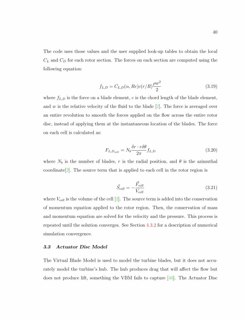
40
The code uses those values and the user supplied look-up tables to obtain the local
CL and CD for each rotor section. The forces on each section are computed using the
following equation:
fL,D = CL,D(α,Re)c(r/R)ρw2
2(3.19)
where fL,D is the force on a blade element, c is the chord length of the blade element,
and w is the relative velocity of the fluid to the blade [2]. The force is averaged over
an entire revolution to smooth the forces applied on the flow across the entire rotor
disc, instead of applying them at the instantaneous location of the blades. The force
on each cell is calculated as:
FL,Dcell= Nb
δr · rδθ2π
fL,D (3.20)
where Nb is the number of blades, r is the radial position, and θ is the azimuthal
coordinate[2]. The source term that is applied to each cell in the rotor region is
~Scell = −~FcellVcell
(3.21)
where Vcell is the volume of the cell [2]. The source term is added into the conservation
of momentum equation applied to the rotor region. Then, the conservation of mass
and momentum equation are solved for the velocity and the pressure. This process is
repeated until the solution converges. See Section 4.3.2 for a description of numerical
simulation convergence.
3.3 Actuator Disc Model
The Virtual Blade Model is used to model the turbine blades, but it does not accu-
rately model the turbine’s hub. The hub produces drag that will affect the flow but
does not produce lift, something the VBM fails to capture [40]. The Actuator Disc
41
Model (ADM) was used previously by Gosset [40] to model the hub. This method
produced accurate results and was applied for the same purpose in this thesis.
ADM uses Actuator Disc Theory, also known as Linear Momentum Theory, to model
the flow field around an aerodynamic object that produces a discontinuity in the
pressure, but not the velocity. The theory uses one-dimensional streamtube analysis
of the flow field. The object (the turbine hub in the case of this thesis) is modeled as
a permeable surface (or porous media) of the same area, known as an Actuator Disc.
The permeable surface allows fluid to pass through the disc but creates a pressure
difference across the disc. The force on the fluid caused by the pressure difference is
representative of the drag force produced by the hub. The pressure difference across
the disc, and subsequently the drag, can be modified by changing the permeability of
the disc.
The permeability constant of the Actuator Disc that is used to represent the hub of
the turbine is required as an input to the model. This value can be determined by
performing control volume analysis on the flow around the turbine hub, as follows.
The necessary assumptions for this analysis are; one-dimensional steady state, incom-
pressible flow. The pressure far downstream in the wake is approximately equal to the
free stream pressure upstream of the actuator disc. The control volume is assumed to
be a stream tube that encompasses the hub. It starts far upstream of the device where
the flow has not been affected by the turbine and ends far downstream of the device
where the velocity of the fluid is uniform in the streamwise direction, see Figure 3.2.
The equation for conservation of mass in a control volume is
∂
∂t
∫C.V.
ρdV +
∫C.S.
ρ~u · ~ndA = 0 (3.22)
where C.V. is the control volume, C.S. is the control surfaces (boundaries), ρ is the
density, ~u is the velocity vector, V is the volume, A is the area, and ~n is the normal
vector. When the ADM assumptions are applied to the equation it simplifies to

42
Figure 3.2: Actuator Disc Model of a turbine using a stream tube analysis [27].
u1A1 = u2A2 = u3A3 (3.23)
where u represents the velocity, A represents the cross sectional area of the stream
tube at a specific location, the subscript 1 refers to a region far upstream of the
Actuator Disc, the subscript 2 refers to the disc, and the subscript 3 refers to the far
wake.
The conservation of momentum equation for a control volume is
∂
∂t
∫C.V.
ρ~udV +
∫C.S.
ρ~u(~u · ~n)dA =
∫C.S.
−P~ndA+
∫C.S.
¯τ · ~ndA+
∫C.V.
ρ~gdV (3.24)
where P is the pressure, ¯τ is the shear stress tensor, and ~g is the gravitational ac-
celeration vector. When the ADM assumptions are applied, the equation simplifies
to
ρu32A3 − ρu12A1 = A2(p
+2 − p−2 ) = FA (3.25)

43
where FA is the force the actuator disc applies to the flow, p−2 is the pressure on
the front of the disc (upstream side), and p+2 is the pressure on the back of the disc
(downstream side).
Since the flow is steady and incompressible, there are no frictional losses, and the flow
is along a streamline, Bernoulli’s Equation can be applied upstream and downstream
of the actuator disc[20].
piρ
+1
2ui
2 + gzi = constant (3.26)
where g is gravitational acceleration, z is the vertical position, and the index i rep-
resents any position along the streamline. The following equations were derived by
assuming there is no elevation change along the stream tube and applying Bernoulli’s
Equation to the upstream side of the actuator disc and the downstream side of the
actuator disc.
p1 +1
2ρu1
2 = p−2 +1
2ρu22 (3.27)
p3 +1
2ρu3
2 = p+2 +1
2ρu22 (3.28)
By subtracting Equation 3.28 from 3.27, applying the assumption that p1 ≈ p3, and
multiplying both sides by A2, the equations become
1
2ρA2(u1
2 − u32) = A2(p−2 − p+2 ) = −FA (3.29)
Next, Equations 3.25 and 3.29 are added, and Equation 3.23 is applied, resulting in
u2 =1
2(u1 + u3). (3.30)
At this point in the derivation it is helpful to define a new variable that represents
the reduction of flow velocity caused by the actuator disc. This variable is called the
Axial Induction Factor, defined as
44
a =u1 − u2u1
(3.31)
such that
u2u1
= 1− a (3.32)
u3u1
= 1− 2a. (3.33)
The power loss to the flowing fluid caused by the pressure drop across the actuator
disc represents the power extracted at the disc (dissipated as a result of the hub) and
it can be calculated as:
P = |FA|u2 =1
2ρA2(u1
2 − u32)u2 =1
2ρu31A2[4a(1− a)2]. (3.34)
The efficiency (η) of the actuator disc can be calculated by comparing P to the total
available power in the flow, Ptotal
Ptotal =1
2ρu1
3A2 (3.35)
η = 4a(1− a)2. (3.36)
The Porous Media Model in Fluent can be used to implement the ADM. The Porous
Media Model adds a momentum source term into the governing momentum equation.
The source term consists of a porous viscous loss term and a porous inertial loss term:
S = −(µ
αu2 + C2
1
2ρu2
2
)(3.37)
where S is the source term, ρ is the density, α is the media permeability, and C2 is
the inertial resistance factor. The coefficients of 1α
and C2 are required inputs to the
Porous Media Model. The relationship between the pressure drop across the porous
media and the source term is

45
∆p = −S∆m (3.38)
where ∆m is equal to the thickness of the disc. The pressure drop calculated by
Actuator Disc theory is
∆p =1
2ρ(u1
2 − u32) (3.39)
and by applying the definition of the axial induction factor it can be rewritten as
∆p =1
2ρu2
2 4a
(1− a). (3.40)
By equating the two expressions for ∆p, Equations 3.38 and 3.40, it can be seen that
∆p =1
2ρu2
2 4a
(1− a)=
(µ
αu2 + C2
1
2ρu2
2
)∆m. (3.41)
The coefficients in front of the u2 terms and the u22 terms are compared, leading to
the following set of equations
1
α= 0 (3.42)
C2 =1
∆m
4a
(1− a). (3.43)
The coefficients required for the Porous Media Model can be determined for any given
value of the induction factor, a. Thus, the model requires a value of the induction
factor, a, as an input.
The hub of a turbine obstructs the flow and results in power dissipation that can
be associated to the drag on the hub. If the power dissipated by the hub is treated
similarly to the power extracted by a turbine (P ), a value of a can be calculated based
on the amount of power that is expected to be dissipated in the wake of the hub. A
relatively small amount of power is dissipated by the turbine’s hub so the efficiency is
assumed to be small, around 20%. A value of 20% efficiency provides a value of the
46
axial induction factor of a = 0.055. For ∆m = 0.035m the inertial resistance factor is
C2 = 6.65159. Using C2 = 6.65159 and 1/α = 0, the Porous Media Model is applied
to model the hub in the MHK turbine simulations in this thesis.
3.4 Open Channel Flow Theory
Open channel flow is perhaps the oldest subdiscipline within fluid mechanics, going
back to irrigation canals in egyptian and roman times. It focuses on the motion of
a liquid flowing under atmospheric pressure due to differences in elevation (potential
energy). The flow is characterized by the height of the liquid (typically water) surface
that is exposed to atmospheric pressure, see Figure 3.3. In open channel flow prob-
lems, the basic force balance is between friction on the (bottom and side) walls and
differences in gravitational potential (or the hydrostatic pressure gradient induced by
it) [20]. The frictional force is a result of a no slip boundary condition at the interface
between the water and the channel walls. This no slip condition leads to a velocity
gradient and subsequently a shear stress at the boundaries. The total frictional force
on the fluid is equal to the shear stress multiplied by the total area of the solid bound-
aries. The hydrostatic pressure difference is created by the gravity and the difference
in free surface height from the inlet to the outlet. Assuming that the channel has a
constant cross section, the difference in height will have an associated difference in
velocity between the inlet and the outlet: as the free surface height decreases, the
cross section of the flow decreases and the velocity has to increase proportionally.
This is necessary to conserve mass.
The important assumptions for a control volume analysis of open channel flow prob-
lems are:
• the free surface is a streamline
• the bottom has a no slip boundary condition
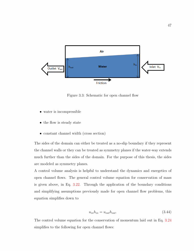
47
Figure 3.3: Schematic for open channel flow
• water is incompressible
• the flow is steady state
• constant channel width (cross section)
The sides of the domain can either be treated as a no-slip boundary if they represent
the channel walls or they can be treated as symmetry planes if the water-way extends
much further than the sides of the domain. For the purpose of this thesis, the sides
are modeled as symmetry planes.
A control volume analysis is helpful to understand the dynamics and energetics of
open channel flows. The general control volume equation for conservation of mass
is given above, in Eq. 3.22. Through the application of the boundary conditions
and simplifying assumptions previously made for open channel flow problems, this
equation simplifies down to
uinhin = uouthout. (3.44)
The control volume equation for the conservation of momentum laid out in Eq. 3.24
simplifies to the following for open channel flows:
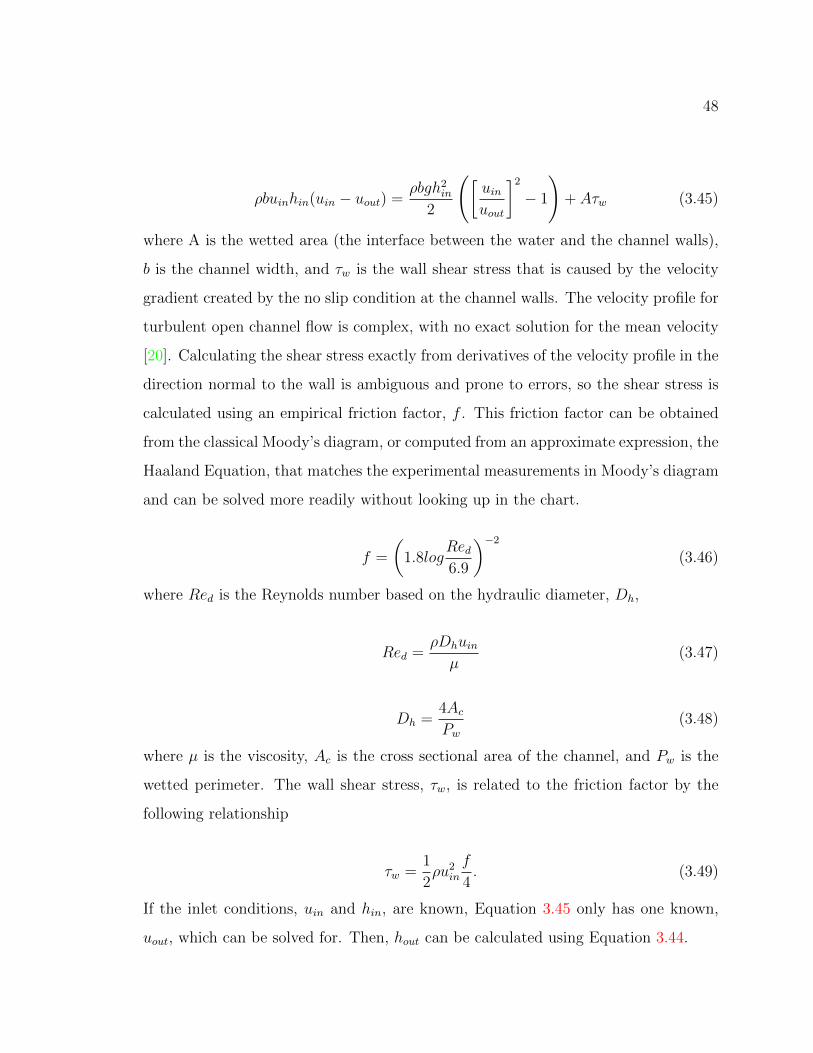
48
ρbuinhin(uin − uout) =ρbgh2in
2
([uinuout
]2− 1
)+ Aτw (3.45)
where A is the wetted area (the interface between the water and the channel walls),
b is the channel width, and τw is the wall shear stress that is caused by the velocity
gradient created by the no slip condition at the channel walls. The velocity profile for
turbulent open channel flow is complex, with no exact solution for the mean velocity
[20]. Calculating the shear stress exactly from derivatives of the velocity profile in the
direction normal to the wall is ambiguous and prone to errors, so the shear stress is
calculated using an empirical friction factor, f . This friction factor can be obtained
from the classical Moody’s diagram, or computed from an approximate expression, the
Haaland Equation, that matches the experimental measurements in Moody’s diagram
and can be solved more readily without looking up in the chart.
f =
(1.8log
Red6.9
)−2(3.46)
where Red is the Reynolds number based on the hydraulic diameter, Dh,
Red =ρDhuinµ
(3.47)
Dh =4AcPw
(3.48)
where µ is the viscosity, Ac is the cross sectional area of the channel, and Pw is the
wetted perimeter. The wall shear stress, τw, is related to the friction factor by the
following relationship
τw =1
2ρu2in
f
4. (3.49)
If the inlet conditions, uin and hin, are known, Equation 3.45 only has one known,
uout, which can be solved for. Then, hout can be calculated using Equation 3.44.

49
Equation 3.45 can be modified to account for the presence of a turbine. This is done
by adding a thrust force into the calculation. The thrust force represents the pressure
difference across the turbine and the frictional forces on the turbine.
ρbuinhin(uin − uout) =ρbgh2in
2
([uinuout
]2− 1
)+ Aτw + Thrust (3.50)
Using the known inlet conditions, this theory can be used to compute the free surface
elevation drop and compare it with the value predicted by numerical simulations for
a given thrust value.
3.5 Numerical Modeling of Open Channel Flows
Modeling the effects of a free surface on the performance of an MHK turbine requires
the combination of two separate models, a model for the turbine and a multiphase
model for the free surface. The theory behind modeling a turbine was already dis-
cussed in Sections 3.2.1 and 3.3.
Prior to combining the two models, it is important to describe in detail the methodol-
ogy used to model the free surface deformation without a turbine. The stability and
accuracy of the free surface model was studied in a simple open channel flow, without
the complexity added by the presence of a turbine. The issues that arose in the spatial
discretization, convergence and accuracy of the free surface deformation could thus
be resolved by comparison with simple channel flow solutions, in the absence of the
MHK turbine.
There are several options for multiphase models that track the free surface loca-
tion: Euler-Euler Approach, Volume of Fluid (VOF) model, Mixture Model, and the
Eulerian-Lagragian Model. In the Euler-Euler Approach and the Mixture Model, the
different phases are assumed to be interpenetrating continua and are primarily used
for phases that are mixed together, like gas bubbles in a liquid or liquid droplets in a
gas flow [41]. The Eulerian-Lagragian Model solves a set of momentum and continuity

50
equations for each phase, or for each discrete mass of a phase immersed in the other,
continuous phase, making it the most complex and time consuming multiphase model
[41]. The Volume of Fluid model tracks the average location of the interface between
two phase, without tracking discrete fluid elements (as in the Eulerian-Lagragian).
It is commonly used primarily for slug flows, stratified flows, and free-surface flows,
where the complexity of the phase distribution is too high for the E-L model and
the free surface location can be describe effectively by an average position without
the specifics of the local deformation within a grid cell. Since the Volume of Fluid
model was less computationally expensive than the Eulerian-Lagrangian Model, and
tracks the fluid interfaces with adequate accuracy for the purpose of this study (sur-
face tension is not important and only the average free surface location plays a role in
the energetics of the open-channel flow), it was used for modeling MHK- free surface
interactions in this thesis.
3.5.1 Volume of Fluid Theory
The Volume of Fluid (VOF) model was developed by C. W. Hirt and B. D. Nichols
[42]. They postulated that problems involving free boundaries that underwent large
deformations would be solved more easily using an Eulerian method than a Lagrangian
method. They used the local volume fraction, Φ, to represent the fractional volume
of a cell occupied by a specific fluid. The evolution of the variable is tracked in the
numerical grid.
This method to implemented in ANSYS Fluent, introducing a variable for each phases’
volume fraction, αq , where q represents the index of each phase present in the flow.
The volume fraction is calculated using a volume fraction continuity equation:
1
ρq
[∂
∂t(αqρq) +5 · (αqρq ~vq) = Sαq +
n∑p=1
mpq − mqp
](3.51)
where ρq is the density of the qth fluid, ~vq is the velocity of the qth fluid, Sαq is a
51
mass source term, mqp is the mass transfer from fluid q to fluid p and mpq is the
mass transfer from fluid p to fluid q [41]. For open channel flows this equation can be
simplified greatly because there is no mass source, no mass transfer between fluids,
and the flow is incompressible. In this case, the continuity equation for the phase q
simplifies down to [42]:
∂
∂t(αqρq) +5 · (αqρq ~vq) = 0. (3.52)
A single momentum equation is solved for the problem and the resulting velocity is
applied to all phases within a grid cell.
∂
∂t(ρ~v) +5 · (ρ~v~v) = −5 p+5 · [µ(5~v +5~vT )] + ρ~g + ~F (3.53)
where p is the pressure, µ is the viscosity, g is gravitational acceleration, and F are ex-
ternal forces. The material properties of the fluid inside each cell are calculated using
the local value of the volume fraction and the material properties of each individual
fluid,
ρ =∑
αqρq (3.54)
µ =∑
αqµq. (3.55)
3.5.2 Initial Conditions
Open channel flow problems require a very specific set of initial conditions and bound-
ary conditions that if chosen incorrectly, will produce unphysical results. The VOF
model is very sensitive to the initial conditions used to initialize the problem [43]. For
example, the volume fraction of water must be set as 1 in the portion of the domain
that will likely be occupied by water. This is accomplished by marking the region of
water in the Region Adaption dialog box and setting the volume fraction of water in
that region as 1, see Figures 3.4 and 3.5. If this is not done, the water will simply

52
enter the domain from the inlet and cascade to the bottom of the channel, because
there is no hydrostatic pressure present throughout the domain to maintain the water
height at the inlet, creating instabilities.
Figure 3.4: The Region Adaption dialog box is used to specify the initial water region
3.5.3 Boundary Conditions
There are several different boundary conditions that can be used for the top, inlet,
and outlet of an open channel flow domain.
The Volume of Fluid implementation in Fluent has an open channel flow option that
allows the user to select boundary conditions specifically designed for open channel
flow simulations. In order to use those boundary conditions, the water inlet and the
air inlet must be combined into one multiphase inlet, and the water outlet and air
outlet must be combined into one multiphase outlet. Once this is done, the inlet
conditions available for the open channel flow option are a mass flow rate inlet and a
pressure inlet. The mass flow rate inlet requires the user to specify the mass flow rate
of air, the mass flow rate of water, the channel’s bottom height, and the free surface
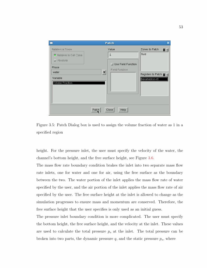
53
Figure 3.5: Patch Dialog box is used to assign the volume fraction of water as 1 in a
specified region
height. For the pressure inlet, the user must specify the velocity of the water, the
channel’s bottom height, and the free surface height, see Figure 3.6.
The mass flow rate boundary condition brakes the inlet into two separate mass flow
rate inlets, one for water and one for air, using the free surface as the boundary
between the two. The water portion of the inlet applies the mass flow rate of water
specified by the user, and the air portion of the inlet applies the mass flow rate of air
specified by the user. The free surface height at the inlet is allowed to change as the
simulation progresses to ensure mass and momentum are conserved. Therefore, the
free surface height that the user specifies is only used as an initial guess.
The pressure inlet boundary condition is more complicated. The user must specify
the bottom height, the free surface height, and the velocity at the inlet. These values
are used to calculate the total pressure po at the inlet. The total pressure can be
broken into two parts, the dynamic pressure q, and the static pressure ps, where

54
Figure 3.6: Dialog Box for Open Channel Flow option Pressure Inlet
po = q + ps (3.56)
q =ρ− ρ0
2V 2 (3.57)
ps = (ρ− ρ0)|~g|((g ·~b) + ylocal) (3.58)
ρ is the density of the mixture in a cell, ρ0 is the reference density (which is the
density of the lightest fluid), V is the velocity magnitude, ~g is the gravity vector, g
is the unit vector of gravity, ~b is the position vector of the centroid of a cell with
respect to a reference location, and ylocal is the vertical distance from the free surface
to the reference location. This creates a hydrostatic pressure profile at the inlet for
the water. The speed of the water is set in the dialog box seen in Figure 3.6. Similar
to the mass flow rate boundary condition, the free surface level is allowed to change
in order to conserve mass and momentum.
Another inlet condition was manually created. The intent was to prescribe a velocity
55
to the water but not to the air. This was done by splitting the inlet into two separate
inlets, one specifically for water, and one specifically for air. A mass flow inlet for
the water inlet and a pressure inlet for the air inlet were then assigned. One issue
that arises with this boundary condition is the free surface height at the inlet is not
allowed to fluctuate.
The options considered for the outlet boundary condition were different variations of
a pressure outlet. For pressure outlets, the open channel flow option for the VOF
model provides two different methods for specifying pressure. One is by prescribing
the bottom height and the free surface height at the outlet in a similar fashion to what
was done in the pressure inlet boundary condition. The other is using the pressure
from a neighboring cell as the pressure at the boundary. A third method for pressure
specification was also applied, writing a User Defined Function (UDF) to prescribe
a hydrostatic pressure profile at the outlet. This method was successfully used in a
similar previous study [18].
For the top boundary, a pressure inlet, pressure outlet, or symmetry boundary can
be applied.
Given the significant uncertainty in exact meaning of certain values and variables used
in the boundary conditions implemented for VOF and open channel flow, different
simulations were conducted using combinations of these inlet and outlet conditions.
This provided control over what were the exact constraints imposed by the boundary
conditions used in the “production” runs in this thesis. The general findings of those
simulations were;
• The mass flow rate inlet and pressure inlet open channel flow boundary con-
ditions allowed for fluctuations in the free surface height. This provided an
accurate free surface elevation change when paired with certain outlet condi-
tions, but the velocity profiles in air were unphysical.
• In simulations with two separate inlets, one for air and one for water, the free
56
surface height at the inlet was fixed, so the free surface did not have a constant
downward slope as would be expected by theory. However, since the air inlet
was a pressure inlet (not assigned a velocity or mass flow rate) the velocity in
the air most accurately represented what would be expected physically.
• When using a UDF for the outlet pressure specification method, the outlet free
surface height was fixed and regardless of the inlet boundary condition, the inlet
free surface height was also fixed, therefore no equilibrium could be reached to
balance the momentum lost to friction on the bottom of the channel. This
produced inaccurate modeling of the free surface.
• Simulations that used the neighboring cell for the pressure specification method
exhibited convergence problems. The neighboring cell boundary condition al-
lowed fluctuations in the free surface height at the outlet. When combined with
an open channel flow inlet condition, the entire free surface height would change,
such that it no longer represented the flow being modeled.
• Simulations using the free surface height and the bottom height in the pressure
specification method for the pressure outlet fixed the free surface height at
the outlet. When combined with the open channel flow inlet conditions, this
boundary condition produced a free surface with a constant slope that was fixed
at the outlet, similar to what is expected of open channel flows.
• When the symmetry boundary condition was applied to the top boundary, the
air moved at a constant velocity throughout the entire domain, which is not
physical. However, it has negligible effects on the free surface behavior and the
turbine’s performance.
• When the pressure inlet and pressure outlet boundary conditions were applied
to the top boundary and paired with certain velocity inlet and outlet boundary
57
conditions, they provided a velocity gradient in the air similar to what would
be expected for an open channel flow. The air had the same velocity as the
water at the free surface, and the velocity decayed further away from the free
surface. However, the inlet and outlet velocity boundary conditions required
to produce that velocity gradient in the air did not accurately model the free
surface behavior.
Since the purpose of this study is to determine how a free surface affects MHK turbine
behavior, it was decided that proper modeling of the free surface was more important
than proper modeling of the air’s velocity profile, because the air’s velocity far above
the free surface has negligible effects on the turbine performance.
It was concluded that the most appropriate boundary conditions for simulating open
channel flows were symmetry for the top, Pressure Inlet with the Open Channel Flow
Option for the inlet, and Pressure Outlet with the Open Channel Flow Option for the
outlet. The pressure specification method for the outlet was the free surface height
and the bottom height. The symmetry boundary condition was selected for the top
boundary because when combined with certain velocity inlet and outlet conditions,
it accurately modeled the change in the free surface height. Also, the symmetry
boundary condition produced better convergence in a simulation of a 10 meter long
test channel, see Table 3.1. Even though the air mass flow rate boundary condition
performed well, it was not desirable to guess the mass flow rate of the air, so the
pressure inlet was selected.
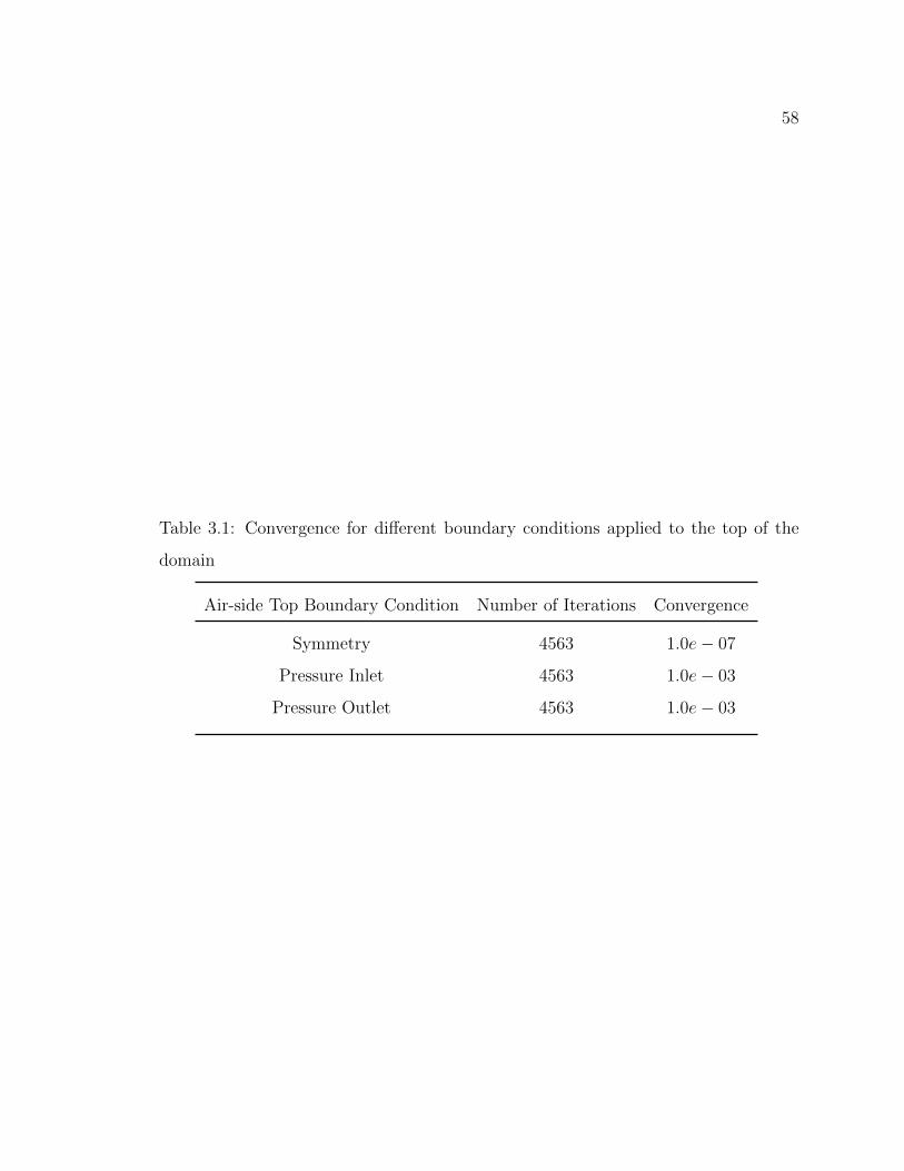
58
Table 3.1: Convergence for different boundary conditions applied to the top of the
domain
Air-side Top Boundary Condition Number of Iterations Convergence
Symmetry 4563 1.0e− 07
Pressure Inlet 4563 1.0e− 03
Pressure Outlet 4563 1.0e− 03
59
Chapter 4
NUMERICAL MODELING
4.1 Meshing
The process to setup the numerical simulations that provides us the insight into the
flow dynamics studied in this thesis, starts with defining the flow domain and creating
a spatial discretization in which the equations of motion can be numerically solved.
The domain is divided into smaller volumes called cells or elements, such that the
flow variables take discrete values inside the cells, or at the surfaces between the cells
(in case of fluxes). The flow domain used for in this thesis can be seen in Figure
4.1, including the location of the free surface and of the MHK turbine. The CFD
simulations take the governing differential equations, convert them to equations in
differences (with discrete instead of continuous variables) and solve them in the small
control volumes that are the grid cells.
The accuracy of the solution is related to the number of mesh cells. Normally, it
is a direct relationship, more cells lead to a more accurate solution. However, an
increase in the number of cells also increases the computational time. The key to
an efficient and accurate numerical discretization of the flow domain is to balance
the need for higher spatial resolution in regions with large variations in the fluid
variables (high gradients) with lower resolution in regions where the fluid variables
are evolving smoothly (low values of the gradients). In the numerical simulations used
in this thesis, there were always two regions of the flow that required a fine mesh:
the turbine wake, and the free surface, see Figure 4.2. The most delicate step in the
preprocessing of the numerical simulations is to generate a high quality mesh, with
sufficient resolution (high grid count) in the regions were the flow solution requires
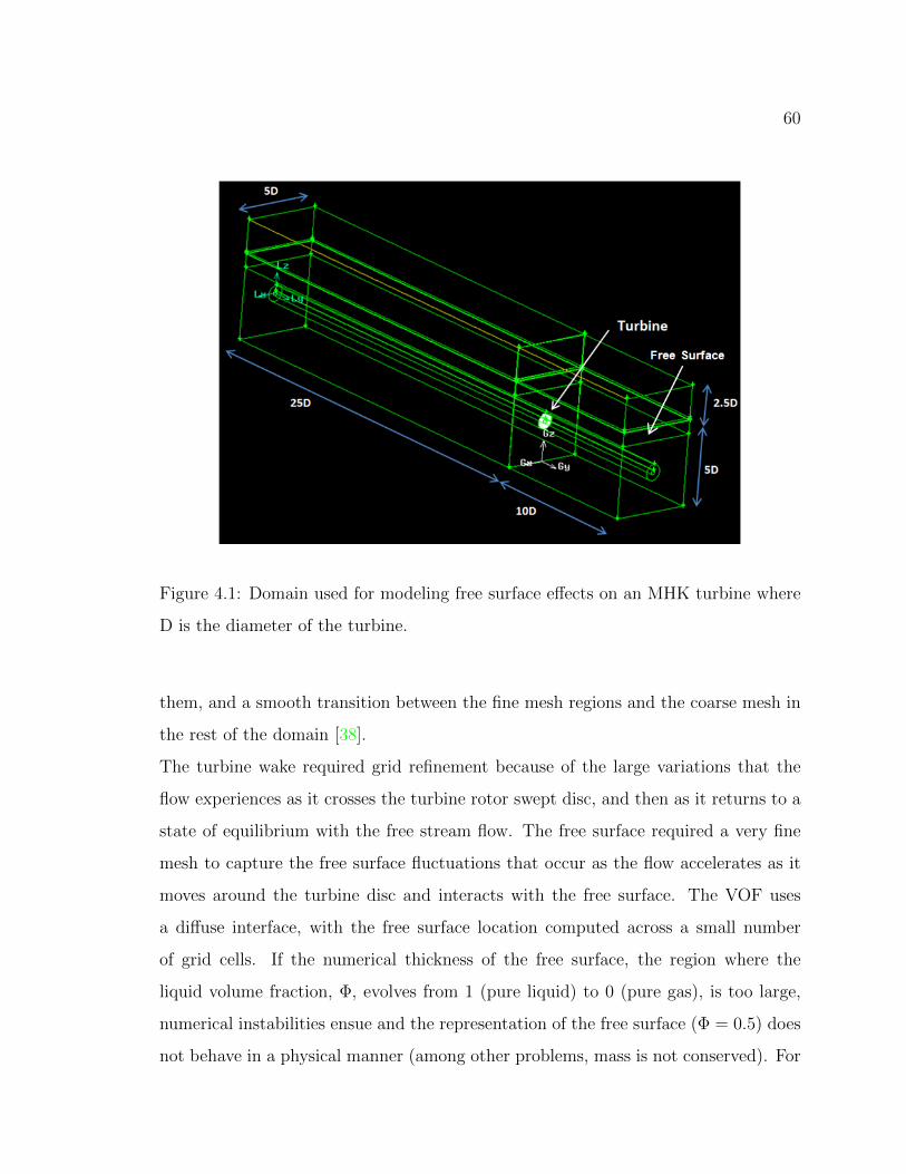
60
Figure 4.1: Domain used for modeling free surface effects on an MHK turbine where
D is the diameter of the turbine.
them, and a smooth transition between the fine mesh regions and the coarse mesh in
the rest of the domain [38].
The turbine wake required grid refinement because of the large variations that the
flow experiences as it crosses the turbine rotor swept disc, and then as it returns to a
state of equilibrium with the free stream flow. The free surface required a very fine
mesh to capture the free surface fluctuations that occur as the flow accelerates as it
moves around the turbine disc and interacts with the free surface. The VOF uses
a diffuse interface, with the free surface location computed across a small number
of grid cells. If the numerical thickness of the free surface, the region where the
liquid volume fraction, Φ, evolves from 1 (pure liquid) to 0 (pure gas), is too large,
numerical instabilities ensue and the representation of the free surface (Φ = 0.5) does
not behave in a physical manner (among other problems, mass is not conserved). For

61
all the simulations in this thesis (Reynolds number= 5 × 10⁵ - 2 × 10⁶), the results
of which are presented in Section 5.1, the cell size near the free surface in the plane
normal to the flow had to be less than 0.1m to accurately predict the decay in free
surface height due to the friction on the channel floor. If the mesh size was larger,
the free surface would not behave as theory predicted and mass was not conserved,
see Figure 4.3.
Figure 4.2: The mesh of the domain on a plane normal to the flow direction
A fine structured rectangular mesh was the preferred meshing scheme near the free
surface. This allowed for the resolution of small variations in the free surface height.
62
The region of the domain comprising of air was not subject to large flow variations,
so a coarse mesh was used to help minimize the number of cells in the simulation. An
unstructured triangular pave mesh was used to transition from the coarse mesh on the
air side to the fine mesh at the free surface. The unstructured mesh in the transitional
region had a skewness below 0.24. Skewness is a measure of mesh quality that ranges
between 0 and 1. Generally it is good practice to keep the maximum skewness for any
element in a mesh below 0.8. The meshes used in numerical simulations described in
this thesis all had skewness values below 0.55.
The boundary layer that developed at the bottom of the channel could not realis-
tically captured in this simulation, and the results did not depend on the velocity
gradient in that part of the domain being realistic, therefore a coarse mesh was used
to reduce the size of the computations, in memory and CPU requirements, reserving
the computing power available to where it had the most impact on the physics stud-
ied. An unstructured mesh was used in the transition region between the turbine,
where the mesh was quite fine, and the bottom, where it was coarse. A sizing function
was applied to control the cell growth in the mesh, between the turbine disc and the
bottom wall.
4.2 Numerical Settings
There were numerous simulations performed in the course of this thesis. The following
is a description of the methodology used for the numerical modeling. Several of the
values such as inlet velocity, turbine rotational speed, turbine vertical position, and
turbulence length scales, were varied based on the size of the turbine, the depth
and width of the channel, etc., to investigate the effect of different non-dimensional
parameters, such as the Tip Speed Ratio, the Reynolds number, the turbine depth to
diameter ratio, the blockage ratio, etc. We used a Pressure-Based, Steady State Solver
with an Absolute Velocity Formulation as settings in all simulations. The solution
was run to convergence at approximately 5× 10⁻⁶, see Section 4.3.2.
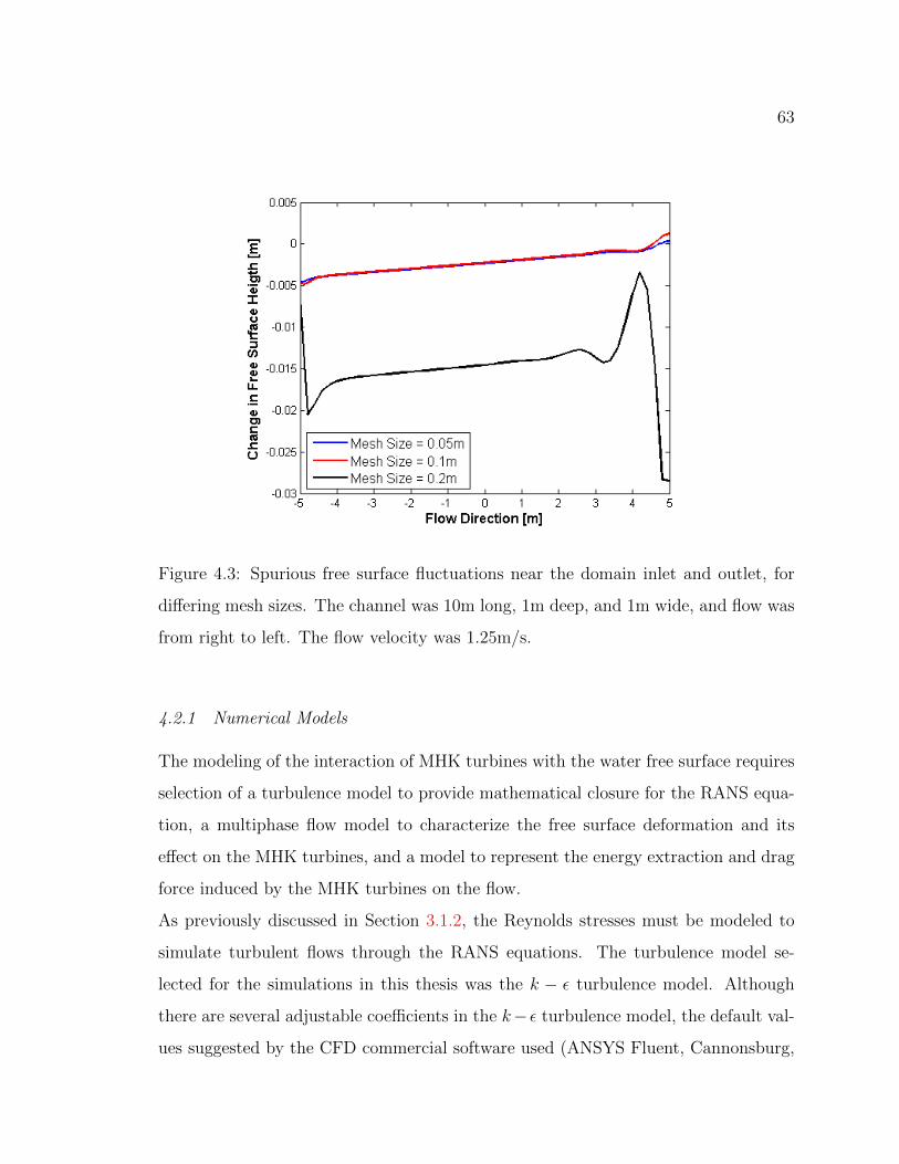
63
Figure 4.3: Spurious free surface fluctuations near the domain inlet and outlet, for
differing mesh sizes. The channel was 10m long, 1m deep, and 1m wide, and flow was
from right to left. The flow velocity was 1.25m/s.
4.2.1 Numerical Models
The modeling of the interaction of MHK turbines with the water free surface requires
selection of a turbulence model to provide mathematical closure for the RANS equa-
tion, a multiphase flow model to characterize the free surface deformation and its
effect on the MHK turbines, and a model to represent the energy extraction and drag
force induced by the MHK turbines on the flow.
As previously discussed in Section 3.1.2, the Reynolds stresses must be modeled to
simulate turbulent flows through the RANS equations. The turbulence model se-
lected for the simulations in this thesis was the k − ε turbulence model. Although
there are several adjustable coefficients in the k− ε turbulence model, the default val-
ues suggested by the CFD commercial software used (ANSYS Fluent, Cannonsburg,

64
PA) were used. It is possible that those coefficients can be fine-tuned for the specific
conditions in MHK turbine flows, but that would require detailed laboratory experi-
ments, at a scale representative of the turbulence in this application (Re ≈ 106−107),
which is currently unavailable in the open literature. While more refined coefficients
may modify some of the results in this thesis quantitatively, typically by a few per-
centage points, the qualitative results that characterize the physics of these flows will
remain relevant.
The dialog box shown in Figure 4.4 presents the input for the numerical implemen-
tation of the multiphase model selected for use in this thesis, the Volume of Fluid
(VOF) model. Section 3.5 includes the results from preliminary simulations run for
the purpose of understanding the features of the VOF model and how to best use them
for the investigation of MHK turbine-free surface interactions. The setting selected
for the model can be seen in Table 4.1.
Table 4.1: Volume of Fluid Settings
Number of Phases 2
Scheme Implicit
Body Force Formulation Implicit Body Force
Options Open Channel Flow
The turbine model selected was the Virtual Blade Model (VBM). For a full explana-
tion of VBM refer to Section 3.2.1 and reference [2]. The dialog box for VBM can
be seen in Figure 4.5. The setting for the dialog box can be seen in Table 4.2. The
turbine modeled was the DOE Reference Model 1 [44]. It is two-bladed rotor and
operates at an optimal tip speed ratio (TSR) of 7.
TSR =ωR
U(4.1)
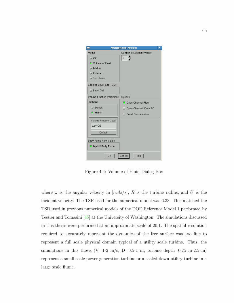
65
Figure 4.4: Volume of Fluid Dialog Box
where ω is the angular velocity in [rads/s], R is the turbine radius, and U is the
incident velocity. The TSR used for the numerical model was 6.33. This matched the
TSR used in previous numerical models of the DOE Reference Model 1 performed by
Tessier and Tomasini [45] at the University of Washington. The simulations discussed
in this thesis were performed at an approximate scale of 20:1. The spatial resolution
required to accurately represent the dynamics of the free surface was too fine to
represent a full scale physical domain typical of a utility scale turbine. Thus, the
simulations in this thesis (V=1-2 m/s, D=0.5-1 m, turbine depth=0.75 m-2.5 m)
represent a small scale power generation turbine or a scaled-down utility turbine in a
large scale flume.
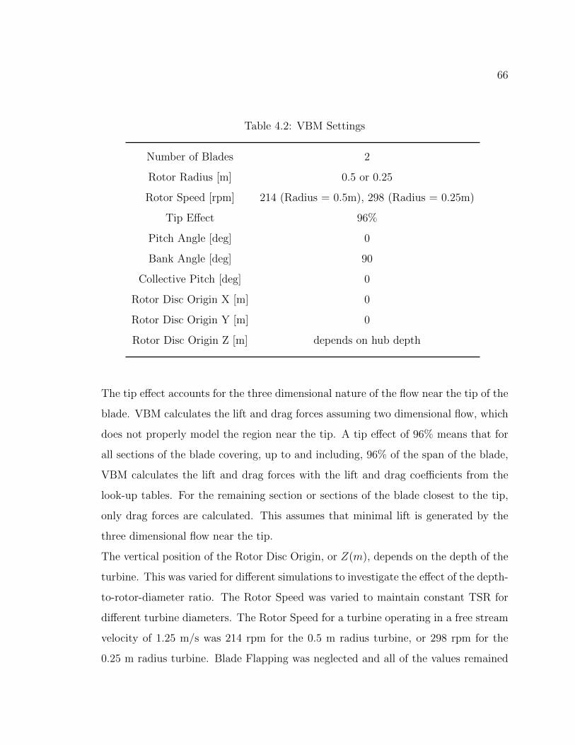
66
Table 4.2: VBM Settings
Number of Blades 2
Rotor Radius [m] 0.5 or 0.25
Rotor Speed [rpm] 214 (Radius = 0.5m), 298 (Radius = 0.25m)
Tip Effect 96%
Pitch Angle [deg] 0
Bank Angle [deg] 90
Collective Pitch [deg] 0
Rotor Disc Origin X [m] 0
Rotor Disc Origin Y [m] 0
Rotor Disc Origin Z [m] depends on hub depth
The tip effect accounts for the three dimensional nature of the flow near the tip of the
blade. VBM calculates the lift and drag forces assuming two dimensional flow, which
does not properly model the region near the tip. A tip effect of 96% means that for
all sections of the blade covering, up to and including, 96% of the span of the blade,
VBM calculates the lift and drag forces with the lift and drag coefficients from the
look-up tables. For the remaining section or sections of the blade closest to the tip,
only drag forces are calculated. This assumes that minimal lift is generated by the
three dimensional flow near the tip.
The vertical position of the Rotor Disc Origin, or Z(m), depends on the depth of the
turbine. This was varied for different simulations to investigate the effect of the depth-
to-rotor-diameter ratio. The Rotor Speed was varied to maintain constant TSR for
different turbine diameters. The Rotor Speed for a turbine operating in a free stream
velocity of 1.25 m/s was 214 rpm for the 0.5 m radius turbine, or 298 rpm for the
0.25 m radius turbine. Blade Flapping was neglected and all of the values remained

67
Figure 4.5: Virtual Blade Model Dialog Box
zero since the rotor blades were considered rigid. The Rotor Disc Bank Angle and
the Pitch Angle describes the rotors alignment relative to the coordinate system, see
Figure 4.6. Since the flow was in the -Y direction the Rotor Disc Pitch Angle was 0◦
and the Rotor Disc Bank Angle was 90◦.
VBM requires some of the blade’s geometry as an input to the model, Table 4.3
shows the necessary data. The blade was divided into 20 blade sections (or blade
elements) which correspond to the Section Numbers. A look-up table for CL and CD
as a function of the angle of attack and Reynolds number, was also provided for each
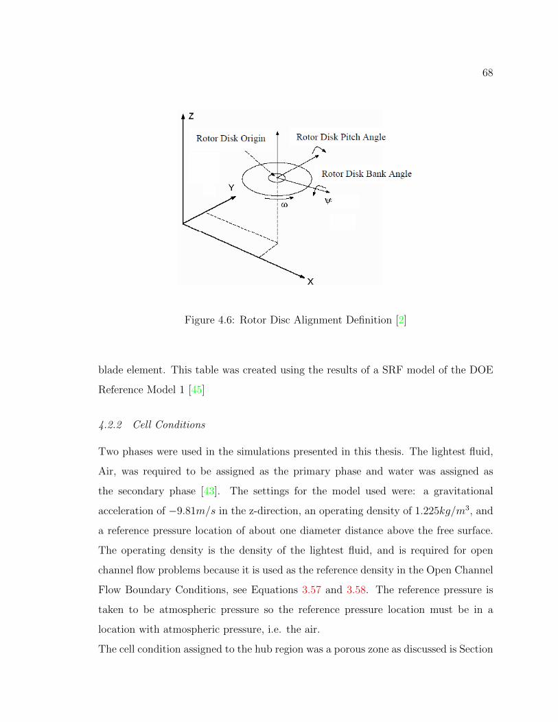
68
Figure 4.6: Rotor Disc Alignment Definition [2]
blade element. This table was created using the results of a SRF model of the DOE
Reference Model 1 [45]
4.2.2 Cell Conditions
Two phases were used in the simulations presented in this thesis. The lightest fluid,
Air, was required to be assigned as the primary phase and water was assigned as
the secondary phase [43]. The settings for the model used were: a gravitational
acceleration of −9.81m/s in the z-direction, an operating density of 1.225kg/m3, and
a reference pressure location of about one diameter distance above the free surface.
The operating density is the density of the lightest fluid, and is required for open
channel flow problems because it is used as the reference density in the Open Channel
Flow Boundary Conditions, see Equations 3.57 and 3.58. The reference pressure is
taken to be atmospheric pressure so the reference pressure location must be in a
location with atmospheric pressure, i.e. the air.
The cell condition assigned to the hub region was a porous zone as discussed is Section
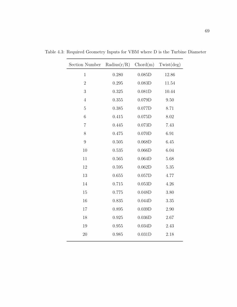
69
Table 4.3: Required Geometry Inputs for VBM where D is the Turbine Diameter
Section Number Radius(r/R) Chord(m) Twist(deg)
1 0.280 0.085D 12.86
2 0.295 0.083D 11.54
3 0.325 0.081D 10.44
4 0.355 0.079D 9.50
5 0.385 0.077D 8.71
6 0.415 0.075D 8.02
7 0.445 0.073D 7.43
8 0.475 0.070D 6.91
9 0.505 0.068D 6.45
10 0.535 0.066D 6.04
11 0.565 0.064D 5.68
12 0.595 0.062D 5.35
13 0.655 0.057D 4.77
14 0.715 0.053D 4.26
15 0.775 0.048D 3.80
16 0.835 0.044D 3.35
17 0.895 0.039D 2.90
18 0.925 0.036D 2.67
19 0.955 0.034D 2.43
20 0.985 0.031D 2.18

70
3.3. The dialog box can be seen in Figure 4.7. The cell condition for the rotor was
a source term. The source term represents the force of the turbine on the fluid. The
force was calculated by VBM.
Figure 4.7: Porous Zone Dialog Box
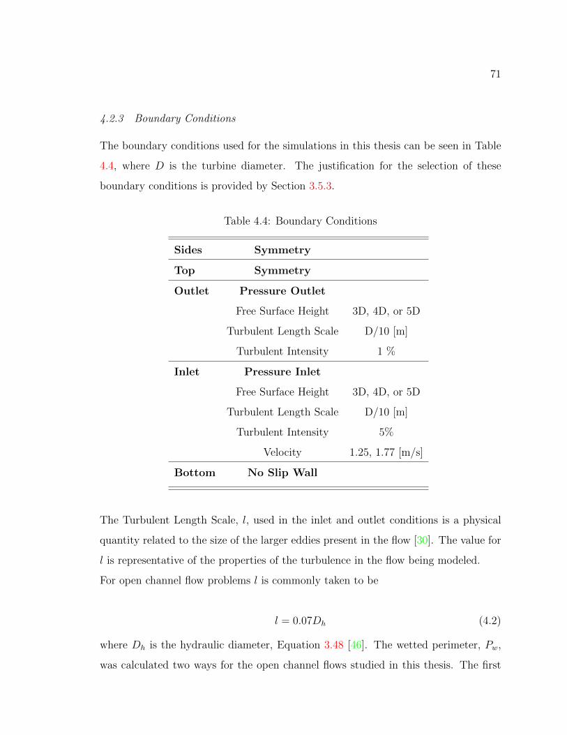
71
4.2.3 Boundary Conditions
The boundary conditions used for the simulations in this thesis can be seen in Table
4.4, where D is the turbine diameter. The justification for the selection of these
boundary conditions is provided by Section 3.5.3.
Table 4.4: Boundary Conditions
Sides Symmetry
Top Symmetry
Outlet Pressure Outlet
Free Surface Height 3D, 4D, or 5D
Turbulent Length Scale D/10 [m]
Turbulent Intensity 1 %
Inlet Pressure Inlet
Free Surface Height 3D, 4D, or 5D
Turbulent Length Scale D/10 [m]
Turbulent Intensity 5%
Velocity 1.25, 1.77 [m/s]
Bottom No Slip Wall
The Turbulent Length Scale, l, used in the inlet and outlet conditions is a physical
quantity related to the size of the larger eddies present in the flow [30]. The value for
l is representative of the properties of the turbulence in the flow being modeled.
For open channel flow problems l is commonly taken to be
l = 0.07Dh (4.2)
where Dh is the hydraulic diameter, Equation 3.48 [46]. The wetted perimeter, Pw,
was calculated two ways for the open channel flows studied in this thesis. The first

72
way was to set Pw as the width of the bottom of the channel with the sides modeled
as symmetry boundaries. The second way was to set Pw equal to the height of the
sides of the channel plus the width of the bottom, which was the length exposed to
water. Given these two definitions for Pw and the different channel depths used in
the simulations, l can have a minimum value of 0.446D or a maximum value of 1.4D
where D is the diameter of the turbine.
Previous simulations of MHK turbine flows conducted in our laboratory used the
chord length of the turbine for the turbulent length scale so that it accurately matched
experimental data [27]. The chord length for the DOE Reference Model 1 is 0.085D.
It was therefore important to determine which turbulent length scale would most
accurately model the physics of an MHK turbine in an open channel. Several different
simulations were conducted with different turbulent length scales ranging from 0.05D
to 1D. The velocity profiles in the region near the turbine and the coefficient of power
for the turbine in each simulation were examined, see Figure 4.8 and Table 4.5.
Table 4.5: Coefficient of Power for Different Turbulent Length Scales
Turbulent Length Scale Coefficient of Power
1D 0.474
0.5D 0.441
0.1D 0.403
0.05D 0.392
The turbine performance, Cp values, obtained for the different turbulent length scales
prescribed at the boundaries were compatible with the range of Cp values calculated by
Tessier and Tomasini [45] for the full size turbine, in the absence of a free surface. The
velocity profiles for the full size turbine [45] showed flow speeds directly downstream of
the hub of the turbine close to the freestream value, suggesting that the correct value of
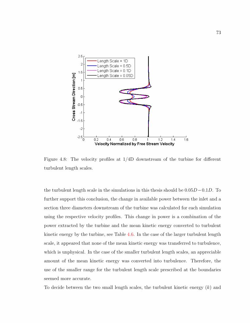
73
Figure 4.8: The velocity profiles at 1/4D downstream of the turbine for different
turbulent length scales.
the turbulent length scale in the simulations in this thesis should be 0.05D−0.1D. To
further support this conclusion, the change in available power between the inlet and a
section three diameters downstream of the turbine was calculated for each simulation
using the respective velocity profiles. This change in power is a combination of the
power extracted by the turbine and the mean kinetic energy converted to turbulent
kinetic energy by the turbine, see Table 4.6. In the case of the larger turbulent length
scale, it appeared that none of the mean kinetic energy was transferred to turbulence,
which is unphysical. In the case of the smaller turbulent length scales, an appreciable
amount of the mean kinetic energy was converted into turbulence. Therefore, the
use of the smaller range for the turbulent length scale prescribed at the boundaries
seemed more accurate.
To decide between the two small length scales, the turbulent kinetic energy (k) and
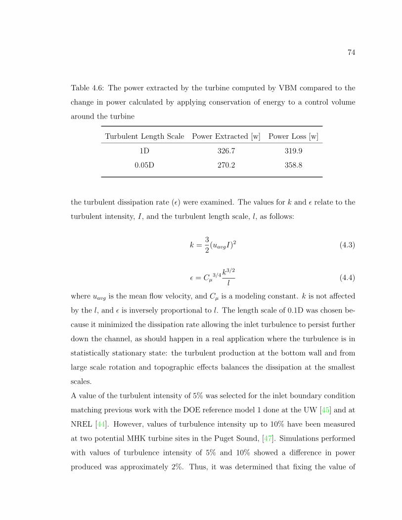
74
Table 4.6: The power extracted by the turbine computed by VBM compared to the
change in power calculated by applying conservation of energy to a control volume
around the turbine
Turbulent Length Scale Power Extracted [w] Power Loss [w]
1D 326.7 319.9
0.05D 270.2 358.8
the turbulent dissipation rate (ε) were examined. The values for k and ε relate to the
turbulent intensity, I, and the turbulent length scale, l, as follows:
k =3
2(uavgI)2 (4.3)
ε = Cµ3/4k
3/2
l(4.4)
where uavg is the mean flow velocity, and Cµ is a modeling constant. k is not affected
by the l, and ε is inversely proportional to l. The length scale of 0.1D was chosen be-
cause it minimized the dissipation rate allowing the inlet turbulence to persist further
down the channel, as should happen in a real application where the turbulence is in
statistically stationary state: the turbulent production at the bottom wall and from
large scale rotation and topographic effects balances the dissipation at the smallest
scales.
A value of the turbulent intensity of 5% was selected for the inlet boundary condition
matching previous work with the DOE reference model 1 done at the UW [45] and at
NREL [44]. However, values of turbulence intensity up to 10% have been measured
at two potential MHK turbine sites in the Puget Sound, [47]. Simulations performed
with values of turbulence intensity of 5% and 10% showed a difference in power
produced was approximately 2%. Thus, it was determined that fixing the value of
75
turbulence intensity at 5% for all simulations in this thesis would eliminate a source of
uncertainty while maintaining the parameter range well grounded at realistic values
for the ultimate application.
The k− ε turbulence model requires the user to specify the turbulent length scale and
the turbulent intensity for reverse flow through an outlet. In the simulations of this
thesis there was no reverse flow, however since the values were required, the length
scale for the outlet was assigned the same length scale as the inlet, and the turbulent
intensity was assigned as 1%. A turbulent intensity of 1% was the approximate
turbulent intensity near the outlet in the numerical simulations.
4.2.4 Solution Methods
Table 4.7 shows the Solution Methods and Solution Controls used in this thesis.
Several of the standard Solution Control Values were changed to aid in the convergence
of the solution as suggested by Section 29.3.2.1 of the ANSYS 14.0 User’s Guide [48].
4.3 Solution
4.3.1 Solution Initialization
Problems solved using VOF require a relatively accurate solution initialization in
order to obtain convergence. This was done by using the Standard Initialization
Method with the initialization variables computed from the Inlet. Once the solution
was initialized, a region of water was patched into the domain, see Section 3.5.2 for
details. Table 4.8 provides the necessary inputs for the region, where D is the diameter
of the turbine.
4.3.2 Convergence
The CFD solver used in the simulations presented in this thesis follows an iterative
process. The convergence of the iterative process can be monitored using residuals.
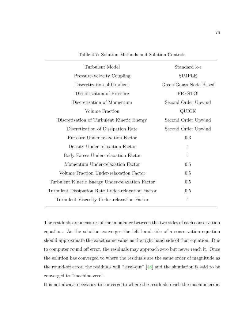
76
Table 4.7: Solution Methods and Solution Controls
Turbulent Model Standard k-ε
Pressure-Velocity Coupling SIMPLE
Discretization of Gradient Green-Gauss Node Based
Discretization of Pressure PRESTO!
Discretization of Momentum Second Order Upwind
Volume Fraction QUICK
Discretization of Turbulent Kinetic Energy Second Order Upwind
Discretization of Dissipation Rate Second Order Upwind
Pressure Under-relaxation Factor 0.3
Density Under-relaxation Factor 1
Body Forces Under-relaxation Factor 1
Momentum Under-relaxation Factor 0.5
Volume Fraction Under-relaxation Factor 0.5
Turbulent Kinetic Energy Under-relaxation Factor 0.5
Turbulent Dissipation Rate Under-relaxation Factor 0.5
Turbulent Viscosity Under-relaxation Factor 1
The residuals are measures of the imbalance between the two sides of each conservation
equation. As the solution converges the left hand side of a conservation equation
should approximate the exact same value as the right hand side of that equation. Due
to computer round off error, the residuals may approach zero but never reach it. Once
the solution has converged to where the residuals are the same order of magnitude as
the round-off error, the residuals will “level-out” [48] and the simulation is said to be
converged to “machine zero”.
It is not always necessary to converge to where the residuals reach the machine error.
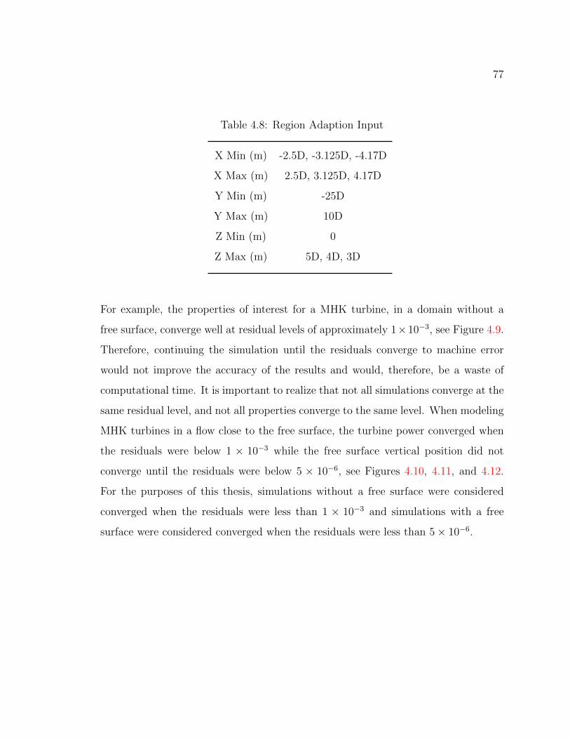
77
Table 4.8: Region Adaption Input
X Min (m) -2.5D, -3.125D, -4.17D
X Max (m) 2.5D, 3.125D, 4.17D
Y Min (m) -25D
Y Max (m) 10D
Z Min (m) 0
Z Max (m) 5D, 4D, 3D
For example, the properties of interest for a MHK turbine, in a domain without a
free surface, converge well at residual levels of approximately 1×10⁻³, see Figure 4.9.
Therefore, continuing the simulation until the residuals converge to machine error
would not improve the accuracy of the results and would, therefore, be a waste of
computational time. It is important to realize that not all simulations converge at the
same residual level, and not all properties converge to the same level. When modeling
MHK turbines in a flow close to the free surface, the turbine power converged when
the residuals were below 1 × 10⁻³ while the free surface vertical position did not
converge until the residuals were below 5 × 10⁻⁶, see Figures 4.10, 4.11, and 4.12.
For the purposes of this thesis, simulations without a free surface were considered
converged when the residuals were less than 1 × 10⁻³ and simulations with a free
surface were considered converged when the residuals were less than 5× 10⁻⁶.
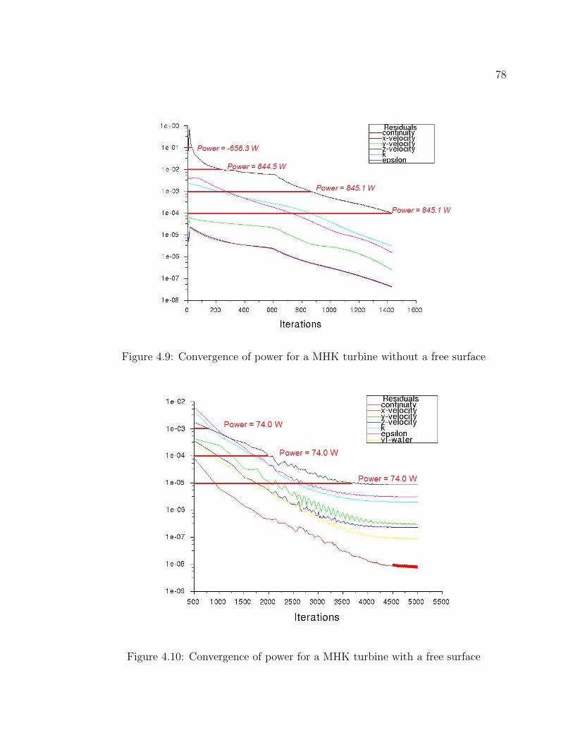
78
Figure 4.9: Convergence of power for a MHK turbine without a free surface
Figure 4.10: Convergence of power for a MHK turbine with a free surface
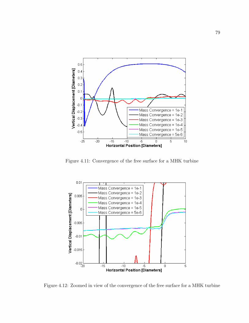
79
Figure 4.11: Convergence of the free surface for a MHK turbine
Figure 4.12: Zoomed in view of the convergence of the free surface for a MHK turbine

80
Chapter 5
RESULTS AND ANALYSIS
5.1 Interactions Between the Free Surface and a Horizontal Axis Tur-bine at Low Blockage Ratios
Five different simulations were performed in an open channel, 5 turbine diameter deep
by 5 diameter wide by 35 diameter long. The depth of the turbine was measured from
the center of the hub to the free surface varying over the five simulations to explore
the hydrodynamics interactions between the MHK turbine flow and the free surface in
a realistic range for confined configurations (flume testing or shallow water estuaries
and rivers): 2.5D, 2D, 1.5D, 1D, and 0.75D. The simulations were performed with
a 1m diameter (D) turbine and a free stream velocity of 1.25m/s in the negative
y-direction. This produced a blockage ratio of 3.14%.
5.1.1 Free Surface Effects on the Wake of a Turbine
The dynamic pressure contours and the velocity profiles for three of the simulations
can be seen in Figure 5.1. Dynamic pressure (q) is defined as:
q =1
2ρv2 (5.1)
where ρ is the local density (φ · ρgas + (1 − φ) · ρlqiuid), and v is the local velocity.
When using velocity contours it is challenging to distinguish between the two different
fluids. Since the two fluids have very different densities and the densities are constant,
the dynamic pressure can be used to both visualize the location of the free surface,
distinguishing between the two phases, and to provide information about the velocity
magnitude in the water flow.

81
Fig
ure
5.1:
Con
tours
ofth
edynam
icpre
ssure
for
diff
eren
ttu
rbin
edep
ths.
Vel
oci
typro
file
sat
diff
eren
tlo
cati
ons
dow
nst
ream
are
also
show
nby
the
bla
ckso
lid
lines
.T
he
scal
esh
ows
the
velo
city
mag
nit
ude
for
wat
erth
atco
rres
pon
ds
toth
edynam
icpre
ssure
conto
urs
.F
low
isfr
omri
ght
tole
ft.

82
When the turbine hub depth is 1.5D (or higher) the wake appears symmetric, however,
as the turbine is moved closer to the free surface the flow becomes asymmetric. The
wake expansion at hub depths of 1D and 0.75D is vertically constrained by the free
surface. This results in an asymmetric wake and an acceleration in the flow directly
above the turbine.
Sun [18] suggests that when a turbine is in close proximity to the free surface the
wake deficit recovery is accelerated, as shown in Figure 2.9. The centerline velocity
was used, mistakenly, to show this trend. By examining Figure 5.2 we show that the
minimum velocity for an asymmetric wake does not occur at the turbine’s centerline
as it does with an axi-symmetric wake. The wake centerline actually deflects towards
the free surface. The minimum wake velocities 20D downstream of the turbine for
the five different turbine depths can be seen in Table 5.1. At 20D downstream the
minimum velocity decreases as the turbine depth decreases, showing that the wake
deficit recovery is hindered, not accelerated, by the asymmetry induced by the free
surface.
Table 5.1: Minimum Wake Velocities 20 Diameters Downstream of the Turbine and
the Respective Decrease in Power Available in the Flow. The Power Available in
the Flow was Based on the Minimum Velocity 20 Diameters Downstream, and the
reference power used was based on the power available for a turbine at a hub depth
of 2.5D
Turbine Depth Minimum Velocity [m/s] Percent Decrease in Available Power
0.075 D 1.0803 5.7
1 D 1.0999 0.5
1.5 D 1.1004 0.3
2 D 1.1016 0
2.5 D 1.1016 0

83
Figure 5.2: The vertical offset of the minimum wake velocity from the centerline
of the turbine. For axi-symmetric flows the minimum wake velocity occurs at the
centerline of the turbine as shown with the Hub Depth = 2.5D.
Figure 5.3 shows the wake deficit for two different hub depths, 0.75D and 2.5D.
The results show the wake persists further downstream for a turbine closer to the
free surface. In flows without a free surface the wake expands out uniformly. The
higher momentum fluid surrounding the wake mixes with the lower momentum fluid
in the wake resulting in an axi-symmetric recovery of the wake. The turbines 2D
and 2.5D away from the free surface behave in this manner. When the turbine is
closer to the free surface, the wake is constrained by the free surface directly above
the turbine. As a result, the upper portion of the wake is not mixed with high
momentum fluid at the same rate as the axi-symmetric wake and, thus, recovers slower
than the bottom portion, with the velocity deficit persisting further downstream and
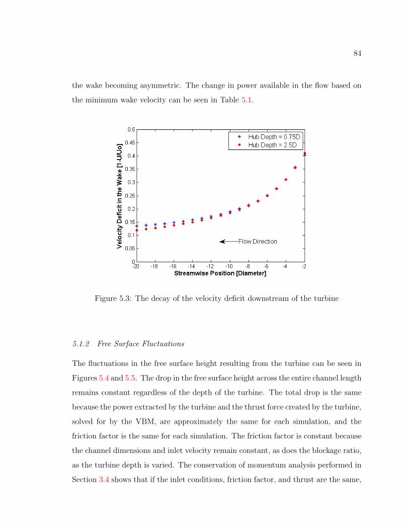
84
the wake becoming asymmetric. The change in power available in the flow based on
the minimum wake velocity can be seen in Table 5.1.
Figure 5.3: The decay of the velocity deficit downstream of the turbine
5.1.2 Free Surface Fluctuations
The fluctuations in the free surface height resulting from the turbine can be seen in
Figures 5.4 and 5.5. The drop in the free surface height across the entire channel length
remains constant regardless of the depth of the turbine. The total drop is the same
because the power extracted by the turbine and the thrust force created by the turbine,
solved for by the VBM, are approximately the same for each simulation, and the
friction factor is the same for each simulation. The friction factor is constant because
the channel dimensions and inlet velocity remain constant, as does the blockage ratio,
as the turbine depth is varied. The conservation of momentum analysis performed in
Section 3.4 shows that if the inlet conditions, friction factor, and thrust are the same,

85
the change in height across the channel will be the same.
The theoretical change in free surface height can be seen in Figure 5.4. This the-
oretical height drop was calculated using the conservation of momentum equation
with the thrust force determined from the different simulations. The magnitude of
the change in height modeled by the simulations and calculated by the theory is the
same, suggesting the simulations behave in a physically sound manner. One reason
the theory and simulations do not match up exactly is the boundary layer at the
bottom of the channel. In the simulations, the boundary layer is not resolved so the
velocity gradient at the bottom of the channel is not accurately modeled leading to
a shear stress value that does not exactly match the friction factor expected for that
Reynolds number flow and channel roughness.
The free surface deformation near the turbine changes for different turbine depths.
Figure 5.4 shows that the amplitude of the fluctuations increase with the decrease in
turbine depth. This is expected because the flow diverted vertically above the turbine
will interact with the free surface. The turbine removes kinetic energy locally from
the flow resulting in a slower fluid speed through the turbine. In order to conserve
mass, some of the flow must be diverted around the turbine. When the turbine is
close to the free surface, the free surface must raise directly upstream of the turbine
to account for the fluid that has been diverted to the region above the turbine.
The turbine removes net potential energy globally from the flow causing a drop in the
free surface directly above the turbine (at the horizontal position of zero). When the
turbine is in close proximity to the free surface, stationary waves form downstream of
the turbine and the waves decay in magnitude as the flow progresses downstream. It
is important to relate the free surface fluctuations to a set of non-dimensional numbers
that control the physics of the MHK turbine-free surface interactions.

86
Figure 5.4: Vertical fluctuations in the free surface along the channel centerline. The
turbine’s horizontal position is represented by the dotted line.
5.2 Non-Dimensional Numbers used to Characterize the Effects of aMHK Turbine on the Free Surface
The non-dimensional number conventionally used to analyze free surface behavior is
the Froude number, see Equation 1.2. The Froude number represents the balance
between the free stream convective velocity and the speed of propagation of gravity
waves at the interface between two fluids of different density, expressed in terms of
the gravitational acceleration constant and a characteristic length scale of the flow (or
more accurately of the wave amplitude). For typical open channel flow problems, the
length scale is the channel depth [20]. However, since there is a turbine in the flow,
several other length scales may be more appropriate, such as the turbine diameter,
the distance from the free surface to the turbine’s tip, or the distance from the free
surface to the center of the hub, see Figure 5.6.
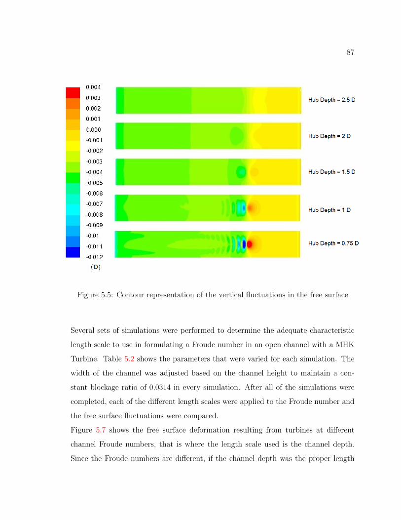
87
Figure 5.5: Contour representation of the vertical fluctuations in the free surface
Several sets of simulations were performed to determine the adequate characteristic
length scale to use in formulating a Froude number in an open channel with a MHK
Turbine. Table 5.2 shows the parameters that were varied for each simulation. The
width of the channel was adjusted based on the channel height to maintain a con-
stant blockage ratio of 0.0314 in every simulation. After all of the simulations were
completed, each of the different length scales were applied to the Froude number and
the free surface fluctuations were compared.
Figure 5.7 shows the free surface deformation resulting from turbines at different
channel Froude numbers, that is where the length scale used is the channel depth.
Since the Froude numbers are different, if the channel depth was the proper length

88
Figure 5.6: Possible characteristic length scales for a MHK turbine in a channel
Table 5.2: Simulation Parameters for Determining the Characteristic Length Scale of
the Froude Number
Parameter Values
Turbine Diameter [D] 1m, 0.5m
Hub depth 2.5 D, 2 D, 1.5 D, 1 D
Channel Depth 5 D, 4 D, 3 D
scale, the free surface fluctuations should be different. However, the fluctuations
are the same. This demonstrates that the free surface fluctuations, at least for low
blockage ratios, are independent of the channel depth. It should be noted that the
Froude number based on channel depth is much less than one for locations were MHK
turbines will be placed, so the channel depth is not expected to affect the flow. For
example, taking the extremes for channel depth (low) and current speed (high) of 5m
deep channel and 2.5m/s current speed, the Froude number is only 0.36, much below

89
the transition to supercritical. The values for channel depth and current speed were
found in reference [49].
Figure 5.7: Free surface fluctuations for different Froude numbers based on channel
depth, where the velocity is 1.25 m/s, the hub depth is 0.75m and the turbine diameter
(D) is 0.5m
Figure 5.8 shows the free surface fluctuations for two different simulations with the
same Froude number when the characteristic length is the tip depth. The fluctuations
are shown in physical values and in non-dimensional form. If the Froude number
based on the tip depth was the non-dimensional parameter governing the free surface
deformations due to the interaction with the MHK turbine, the values presented for
the free surface fluctuations in those two simulations with the same Frtip depth would
be the same, but they are not. Therefore, the tip depth is not a good candidate for
the characteristic length scale in this problem.
Figure 5.9 shows the free surface fluctuations for two different simulations with the
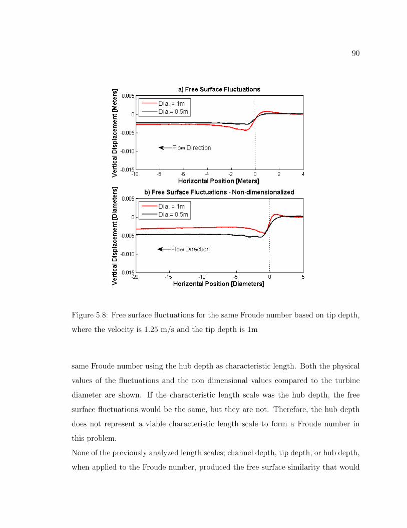
90
Figure 5.8: Free surface fluctuations for the same Froude number based on tip depth,
where the velocity is 1.25 m/s and the tip depth is 1m
same Froude number using the hub depth as characteristic length. Both the physical
values of the fluctuations and the non dimensional values compared to the turbine
diameter are shown. If the characteristic length scale was the hub depth, the free
surface fluctuations would be the same, but they are not. Therefore, the hub depth
does not represent a viable characteristic length scale to form a Froude number in
this problem.
None of the previously analyzed length scales; channel depth, tip depth, or hub depth,
when applied to the Froude number, produced the free surface similarity that would

91
Figure 5.9: Free surface fluctuations for the same Froude number based on hub depth,
where the velocity is 1.25 m/s and the hub depth is 1m
be expected if the Froude number was the only non-dimensional parameter describing
the physics of MHK turbine-free surface interactions. One of the potential problems
with trying to apply a depth as the characteristic length scale is that it does not
account for the size of the turbine. For example, consider a small rock and a large
rock in a river of constant depth, see Figure 5.10. In the figure, the change in the
free surface resulting from a large rock in the center of the river is very noticeable,
however, the fluctuations resulting from all the small rocks around the large rock
are not. Now consider a small fish and a large fish the same distance below the free

92
surface. The large fish would be expected to produce a larger free surface deformation
than the small fish. Therefore, using a characteristic length scale related to the size
of the turbine might produce better results.
Figure 5.10: Free surface fluctuations resulting from a large rock [50]
For a submerged object, the characteristic length scale applied to the Froude number
is the size of the object [51]. This would suggest that the diameter of the turbine
should be used as the characteristic length scale. Figure 5.4 shows the free surface
fluctuations for simulations with the same Froude number based on turbine diameter.
It can be seen that the free surface fluctuations depend on turbine depth. According
to Zhu [51], the free surface fluctuations due to a submerged object, do not just
depend on the Froude number, they also depend on a non-dimensionalized depth of
the object. Thus, if the diameter is the characteristic length scale for the Froude
number another non-dimensional number is also needed to describe depth’s effect on
the fluctuations.
Figure 5.11 shows the free surface fluctuations for six different simulations. The
simulations used the same Froude number that was based on turbine diameter, and
the same non-dimensional depth (dr), where dr is the ratio between the hub depth and
the turbine diameter. The simulations with a 0.5m diameter turbine were performed
with an inlet velocity of 1.25m/s. In order to produce the same Froude number the
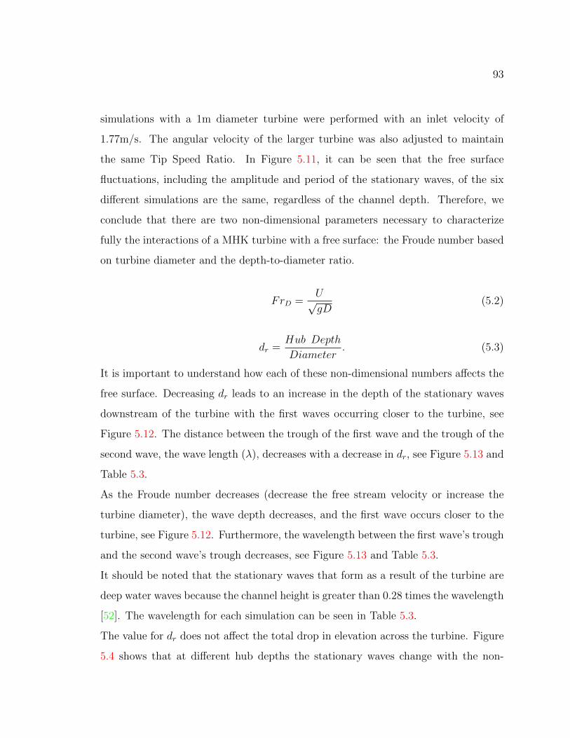
93
simulations with a 1m diameter turbine were performed with an inlet velocity of
1.77m/s. The angular velocity of the larger turbine was also adjusted to maintain
the same Tip Speed Ratio. In Figure 5.11, it can be seen that the free surface
fluctuations, including the amplitude and period of the stationary waves, of the six
different simulations are the same, regardless of the channel depth. Therefore, we
conclude that there are two non-dimensional parameters necessary to characterize
fully the interactions of a MHK turbine with a free surface: the Froude number based
on turbine diameter and the depth-to-diameter ratio.
FrD =U√gD
(5.2)
dr =Hub Depth
Diameter. (5.3)
It is important to understand how each of these non-dimensional numbers affects the
free surface. Decreasing dr leads to an increase in the depth of the stationary waves
downstream of the turbine with the first waves occurring closer to the turbine, see
Figure 5.12. The distance between the trough of the first wave and the trough of the
second wave, the wave length (λ), decreases with a decrease in dr, see Figure 5.13 and
Table 5.3.
As the Froude number decreases (decrease the free stream velocity or increase the
turbine diameter), the wave depth decreases, and the first wave occurs closer to the
turbine, see Figure 5.12. Furthermore, the wavelength between the first wave’s trough
and the second wave’s trough decreases, see Figure 5.13 and Table 5.3.
It should be noted that the stationary waves that form as a result of the turbine are
deep water waves because the channel height is greater than 0.28 times the wavelength
[52]. The wavelength for each simulation can be seen in Table 5.3.
The value for dr does not affect the total drop in elevation across the turbine. Figure
5.4 shows that at different hub depths the stationary waves change with the non-

94
Figure 5.11: Free surface fluctuations for six cases with the same Froude number,
based on the turbine diameter (Fr = 0.565) and the same non-dimensionalized depth
(dr = 1)
dimensionalized depth but the drop in free surface height across the turbine does
not. The Froude number based on turbine diameter, however, does affect the drop
in elevation across the turbine, see Figure 5.14. An increase in the FrD increases the
drop in elevation across the turbine.
This section has shown that the free surface fluctuations are independent of the chan-
nel depth. One possible exception for this conclusion is MHK turbines operating
at high blockage ratios. According to the theory of Whelan [3] and Polagye [8] Cp
increases with the blockage ratio and the Froude number based on channel depth
(channel Froude number). Section 5.3 shows Cp is not affect by the channel depth,
and hence the channel Froude number at low blockage ratios. According to the one-
dimensional flow theory, at very high blockage ratios, greater than 30%, the channel

95
Table 5.3: Free Surface Fluctuations, see Figure 5.13
FrD dr Zmin Ymin λ
0.4 1.5 0.004 0.751 -
1 0.011 0.569 0.973
0.75 0.021 0.533 0.970
0.565 2 0.008 1.085 -
1.5 0.013 0.9731 1.936
1 0.030 0.936 1.890
0.75 0.052 0.862 1.675
Froude number begins to have a significant effect on Cp, see Figure 2.2. However,
very few MHK turbines, specially horizontal axis, will ever be operated at that high
of a blockage ratio because the flow will be significantly altered by the turbine causing
a multitude of environmental effects. The only real purpose for turbines operating
at such high blockage ratios is to hydraulically control a channel. Therefore, for tur-
bines operated in usual conditions, the Froude number based on channel depth has a
negligible effect on the flow. This is discussed in detail in Section 5.5.
5.2.1 Slope Correction
The free surface elevation drop that balances the frictional force on the bottom of the
channel is a function of the flow speed and the channel width, see Equation 3.46. In
these simulations the blockage ratio was kept constant, so the width of the channel
had to change when the channel depth was changed. Equations 3.48 and 3.47 show
that an increase in channel width decreases the hydraulic diameter, which decreases
the Reynolds number, and in turn increases the friction factor. This leads to a higher
momentum loss due to friction that is balanced by a larger difference in free surface

96
Figure 5.12: The depth and position of the stationary wave directly downstream of
the turbine. Red is for a FrD = 0.4 and black is for a FrD = 0.565. The different
lines represent the free surface fluctuations and the symbols represent the maximum
wave depth. −− and ◦ represent a dr = 2. · − · and ∗ represent a dr = 1.5. − and �
represent a dr = 1. · · · and • represent a dr = 0.75.
height across the channel. Table 5.4 shows the theoretical friction factors calculated
for each channel and the friction factors produced by the numerical simulations for
each channel. The trends and approximate magnitude of the friction factors produced
in the simulations match those predicted by theory. The difference in the friction
factors is the result of the simulations not accurately modeling the boundary layer
near the bottom of the channel.

97
Figure 5.13: Explanation of the variables used in Tables 5.3 and 5.6. Zmin is the
depth of the first wave, λ is the wave length between the first wave’s trough and the
second wave’s trough, and Ymin is horizontal distance between the turbine and the
first wave’s trough. Zmax is the height of the deformation of the free surface directly
upstream of the turbine and Ymax is the horizontal distance from the turbine to the
peak of the deformation upstream of the turbine.

98
Figure 5.14: Free surface fluctuations for simulations with the same dr but different
Froude numbers

99
Tab
le5.
4:F
rict
ion
Fac
tors
for
the
diff
eren
tsi
mula
tion
s
Turb
ine
Dia
met
erV
eloci
tyC
han
nel
Dep
thC
han
nel
Wid
thT
heo
reti
cal
Fri
ctio
nF
acto
rSim
ula
ted
Fri
ctio
nF
acto
r
1m1.
77m
/s5m
5m0.
0069
0.01
0
4m6.
25m
0.00
710.
010
3m8.
33m
0.00
730.
0106
1m1.
25m
/s5m
5m0.
0072
0.01
02
4m6.
25m
0.00
74-
3m8.
33m
0.00
77-
0.5m
1.25
m/s
2.5m
2.5m
0.00
790.
0125
2m3.
125m
0.00
810.
0128
1.5m
4.17
m0.
0085
0.01
38

100
The different free surface slopes related to the different friction factors made com-
paring the free surface fluctuations challenging. A slope correction was created to
adjust the free surface slope to match the slope in the simulations performed with a
1m diameter turbine in a channel 5D deep. Figures 5.7, 5.8, 5.9, and 5.11 have had
this slope correction applied. It is important to understand the slope correction is not
scaling the free surface drop resulting from the turbine, it is only accounting for the
free surface drop related to the bottom friction. Figure 5.15 shows a free surface be-
fore and after the slope correction was applied. The elevation drop resulting from the
power extracted by the turbine does not change when the slope correction is applied
nor does the magnitude and period of the stationary waves.
Figure 5.15: Free surface fluctuations with and without the slope correction

101
5.3 The Effects of the Free Surface on the Coefficient of Power at LowBlockage Ratios
The power extracted by the turbine in each simulation was noted and non-dimensionalized
using the free stream velocity, to produce the turbine’s coefficient of power, see Equa-
tion 2.1. The Cp values for simulations performed with a 0.5m diameter turbine can
be seen in Figure 5.16. The Cp values for simulations performed with a 1m diameter
turbine are shown in Figure 5.17.
Figure 5.16: The coefficient of power for simulations performed with a 0.5m diameter
turbine. The simulations were performed with different channel depths and hub
depths.
The coefficients of power for the 0.5m diameter turbine are within ±0.01 for every
channel depth and turbine depth. This is also true for the 1m diameter turbine. There
are no apparent trends between Cp and the channel depth or the hub depth. Thus,
at this blockage ratio, Cp is either negligibly affected or not affected at all by channel

102
Figure 5.17: The coefficient of power for simulations performed with a 1m diameter
turbine. The simulations were performed with different channel depths and hub
depths. � represents the coefficients of power for a 0.5m diameter turbine with
the same number of mesh cells in the wake as the 1m diameter turbine.
depth or turbine depth. The average coefficient of power for the smaller turbine is
0.467 whereas the average Cp for the larger turbine is 0.393. Since these flows have
all of the same non-dimensional numbers they should also have the same Cp.
Upon further examination the difference in Cp was determined to be a result of the
mesh refinement in the turbine wake. Originally, the same mesh size was used in every
simulation. This was to ensure the free surface behavior would be captured identically
for all simulations. When the mesh for the smaller, 0.5m diameter turbine, was refined
to have the same number of mesh elements as the larger turbine, the Cp values for
the two different size turbines matched, however, the free surface fluctuations became
slightly different.

103
For every simulation, it was determined that it was necessary to keep the number of
mesh elements in the wake constant, while maintaining the size of the elements near
the free surface. This was applied by setting the number of mesh elements on the
outside of the rotor to 90 and fixing the mesh size near the free surface to 0.05m. This
produced the same coefficients of power for the two different size turbines and the
same free surface fluctuations for a certain Froude number and Depth-to-Diameter
Ratio, Figure 5.18 and Figure 5.16.
Figure 5.18: Free surface fluctuations for the same Froude number, Fr = 0.565, and
same depth to diameter ratio, dr = 1.5, where the number of mesh cells in the wake
is constant and the size of the mesh cells at the free surface is constant.
5.4 Blockage Ratio Effects on MHK Turbine Performance
The previous sections are dedicated to the study of flows at a low blockage ratio,
similar to what may be seen in the field. However, it is important to understand how

104
the blockage ratio may affect the power produced to ensure flume experiments, which
have higher blockage ratios, are not misrepresenting the amount of power a MHK
turbine can generate. This study is also relevant to turbines in rivers, channels, and
estuaries, where high blockage ratios (and relatively high channel Froude numbers,
Froude number based on channel depth) can be reached.
A preliminary set of simulations were performed at blockage ratios of 3.14%, 5.23%,
and 12.5%. The simulations applied the same methodology seen in Section 4, but
with differing channel sizes. Figure 5.19 shows the resulting free surface fluctuations
for each case and Figure 5.20 shows the power extracted by the turbine in each case.
These simulations were performed with an inlet velocity of 1.25 m/s.
Figure 5.19: Free surface fluctuations for simulations with different blockage ratios.
Figure 5.19 shows increasing the blockage ratio results in an increase in the free surface
drop across the turbine. According to the control volume analysis, the increased
change in free surface height should mean that more power is extracted by the turbine,

105
Figure 5.20: Power extracted by the turbine versus blockage ratio.
however, Figure 5.20 does not show that. After further examination of the entire
simulation, two major problems were identify as the reasons for this discrepancy, a
change in inlet velocity, and a change in the Tip Speed Ratio (TSR) that produces
the maximum coefficient of power.
5.4.1 Changing Inlet Velocities
First, to address the change in inlet velocity it is important to point out that the
inlet boundary condition used in the simulations was specially tailored by Fluent for
open channel flow problems. The inlet boundary condition dialog box asks for the
inlet velocity magnitude, and according to the Fluent User Manual [43], the user
should enter the magnitude of the upstream inlet velocity. Thus, the inlet velocity of
1.25m/s was entered and assumed to be fixed. After studying the velocity contours at
the inlet for each simulation it became apparent that the inlet velocity had changed

106
as the simulations converged. The amount the velocity changed was related to the
blockage ratio. As the blockage ratio increased the amount of inlet velocity variations
increased. The exact reason for this change is still unknown, however, it maybe a
result of assigning a total pressure at the inlet. If the total pressure is fixed at the
inlet and the static pressure increases due to a change in free surface height, the
dynamic pressure must decrease to compensate, decreasing the velocity. The other
inlet boundary condition found to perform well in Section 3.5.3 was the mass flow
rate boundary condition. However, the same problem occurs with that boundary
condition. When the free surface height rises at the inlet, the cross sectional area of
the flow increases so the velocity must decrease to maintain the inlet mass flow rate
of water.
The power extracted is related to the velocity cubed, so it was concluded that the
change in inlet velocity was partially responsible for the inaccurate relationship be-
tween power and blockage ratio seen in Figure 5.20. To correct for this problem the
coefficient of power was used, see Figure 5.21. Cp is the power non-dimensionalized
by the velocity, so Cp is independent of the inlet velocity. Figure 5.21 shows that the
Cp increased with the blockage ratio as expected.
5.4.2 TSR Versus Coefficient of Power
To address the problem of the change in TSR that produces the maximum power,
note that Cp is related to the TSR in such a way that at low TSRs Cp increases as
the TSR increase, but at some point the Cp reaches its maximum value and begins to
decrease with any increase in TSR. To produce maximum power turbines are operated
at the TSR that corresponds to the maximum Cp. The angular velocity of the turbine
and the free stream velocity used in the simulations are set to produce the TSR that
corresponds to the maximum Cp. The free stream velocity is used for calculating the
TSR instead of the turbine’s local velocity because the free stream velocity is known
prior to starting the simulations. As the blockage ratio increases there is less area
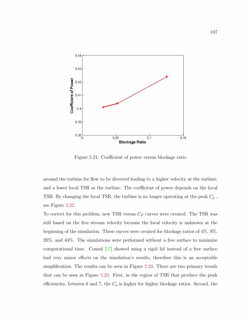
107
Figure 5.21: Coefficient of power versus blockage ratio
around the turbine for flow to be diverted leading to a higher velocity at the turbine,
and a lower local TSR at the turbine. The coefficient of power depends on the local
TSR. By changing the local TSR, the turbine is no longer operating at the peak Cp ,
see Figure 5.22.
To correct for this problem, new TSR versus CP curves were created. The TSR was
still based on the free stream velocity because the local velocity is unknown at the
beginning of the simulation. These curves were created for blockage ratios of 4%, 9%,
20%, and 44%. The simulations were performed without a free surface to minimize
computational time. Consul [37] showed using a rigid lid instead of a free surface
had very minor effects on the simulation’s results, therefore this is an acceptable
simplification. The results can be seen in Figure 5.23. There are two primary trends
that can be seen in Figure 5.23. First, in the region of TSR that produce the peak
efficiencies, between 6 and 7, the Cp is higher for higher blockage ratios. Second, the
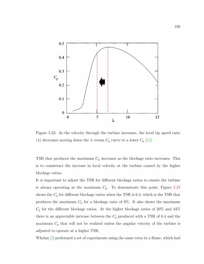
108
Figure 5.22: As the velocity through the turbine increases, the local tip speed ratio
(λ) decreases moving down the λ versus Cp curve to a lower Cp [25]
TSR that produces the maximum Cp increases as the blockage ratio increases. This
is to counteract the increase in local velocity at the turbine caused by the higher
blockage ratios.
It is important to adjust the TSR for different blockage ratios to ensure the turbine
is always operating at the maximum Cp. To demonstrate this point, Figure 5.24
shows the Cp for different blockage ratios when the TSR is 6.4, which is the TSR that
produces the maximum Cp for a blockage ratio of 9%. It also shows the maximum
Cp for the different blockage ratios. At the higher blockage ratios of 20% and 44%
there is an appreciable increase between the Cp produced with a TSR of 6.4 and the
maximum Cp that will not be realized unless the angular velocity of the turbine is
adjusted to operate at a higher TSR.
Whelan [3] performed a set of experiments using the same rotor in a flume, which had
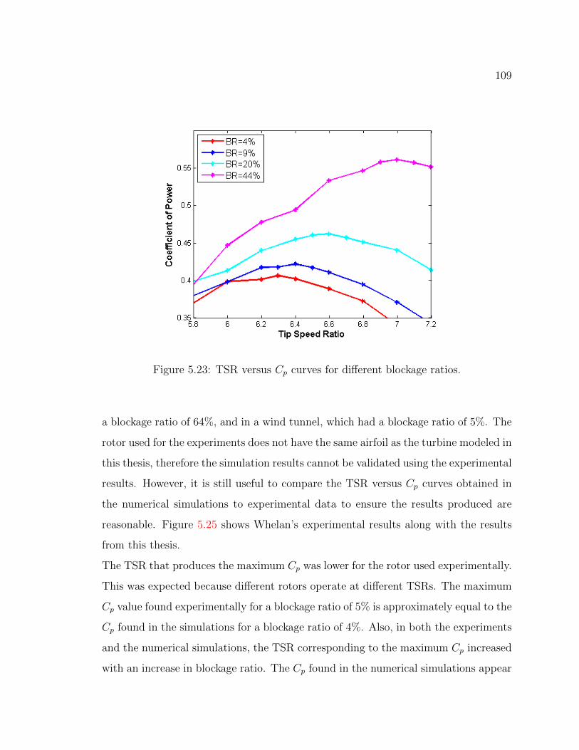
109
Figure 5.23: TSR versus Cp curves for different blockage ratios.
a blockage ratio of 64%, and in a wind tunnel, which had a blockage ratio of 5%. The
rotor used for the experiments does not have the same airfoil as the turbine modeled in
this thesis, therefore the simulation results cannot be validated using the experimental
results. However, it is still useful to compare the TSR versus Cp curves obtained in
the numerical simulations to experimental data to ensure the results produced are
reasonable. Figure 5.25 shows Whelan’s experimental results along with the results
from this thesis.
The TSR that produces the maximum Cp was lower for the rotor used experimentally.
This was expected because different rotors operate at different TSRs. The maximum
Cp value found experimentally for a blockage ratio of 5% is approximately equal to the
Cp found in the simulations for a blockage ratio of 4%. Also, in both the experiments
and the numerical simulations, the TSR corresponding to the maximum Cp increased
with an increase in blockage ratio. The Cp found in the numerical simulations appear

110
Figure 5.24: Cp values for a specific TSR compared with the maximum Cp at different
blockage ratios
to lie in the appropriate range of Cp values found experimentally. Even though this
does not validate the results of this thesis, it demonstrates the results are at least
realistic and provides some confidence to the simulations.
5.5 Numerical Simulations of Experiments Performed with Scaled Tur-bines
At this time, there are several sets of MHK turbine experiments under way at the
University of Washington. It is desirable to use the experimental data to validate the
simulations presented in this thesis.

111
Figure 5.25: TSR versus Cp curves for different blockage ratios found numerically,
compared to experimental data from Whelan[3]. The blocked case refers to experi-
ments performed at a blockage ratio of 64%, and the unblocked case refers to experi-
ments performed at a blockage ratio of 5%
5.5.1 Experiments at Low Reynolds Numbers
When performing experiments using scaled MHK turbines, it is challenging to main-
tain all of the important non-dimensional numbers from full scale turbines. Often
the Reynolds number must be lowered to maintain other non-dimensional numbers
[29]. It is generally considered acceptable to use a lower Reynolds number as long
as it is still in the same asymptotic turbulent regime as the full scale turbine, be-
cause in turbulent flows the coefficients of lift and drag are considered independent
112
for large enough Reynolds number. However, if the chord length based Reynolds
number approaches the transition between laminar flow and turbulence, CL and CD
start to depend heavily on the Reynolds number [53]. This transition occurs around
a Reynolds number of 7 × 10⁴. The dependence of CL and CD on Reynolds number
is suspected to be the result of the formation of Laminar Separation Bubbles (LSB)
on the upper surface of the airfoil [54].
Several scaled experiments were performed in September 2012 using a flume at the
Bamfield Marine Sciences Centre in British Columbia. The Cp values produced ex-
perimentally were much lower than the results predicted by Lawson [44] and Tessier
[45]. One possible reason for the discrepancy in Cp values is the chord length based
Reynolds number was about 7 × 10⁴, so LSBs may have formed on the blade. The
presence of a LSB on the blade reduces the CL and subsequently the power produced.
Figure 5.26 shows a numerical simulation of the turbine blade’s airfoil performed us-
ing a Reynolds number of about 7 × 10⁴. The simulation was performed using the
Transitional SST turbulence model and near wall treatment. The transitional model
was selected since the flow at the leading edge of the blade was assumed to be laminar
and then transitioned to turbulent as it flowed along the airfoil. For an explanation
of the Transitional SST model and the near wall treatment see reference [46]. Fig-
ure 5.26 shows reverse flow on the upper surface of the airfoil. The area of reverse
flow is believed to be a laminar separation bubble since the flow re-attaches further
downstream on the airfoil. This supports the hypothesis of LSB causing the lower Cp
values seen experimentally.
In order to have the experimental data properly model the flow around a full size
turbine, the turbine blade used in the experiments is going to be changed to an airfoil
that operates better at low Reynolds numbers and produces the same Cp as the full
size turbine. Since the experiments will have the same Cp as a full size turbine, the
simulations in this section of the thesis can be performed using the same CL and CD
look-up table used in the previous sections.

113
Figure 5.26: x-velocity contours for flow around an airfoil at a Reynolds number of
7× 10⁴ and an angle of attack of 8.7◦.
5.5.2 Simulation Parameters
Table 5.5 shows the list of parameters for the experiments that are to be performed
with the new airfoil. The experiments will be performed in two different water flumes,
one at the University of Washington (UW) and the other at the Bamfield Marine
Sciences Centre in British Columbia. The UW flume is about 0.6m deep and can
operate at a velocity of 0.6 m/s. The Bamfield flume is about 0.9m deep and can
operate at a velocity of either 0.6m/s or 1.2m/s. Two turbines of different diameters,
0.3m and 0.45m, have been constructed for the experiments.
It proved challenging to duplicate the experiments exactly using numerical simula-
tions. Specifically, simulation runs with an inlet velocity less than 1m/s did not
converge, so an alternative method was needed. The experimental parameters were
non-dimensionalized into; the Tip Speed Ratio (TSR), Reynolds number (Re), chan-
nel Froude number (Frc), Froude number based on turbine diameter (FrD), Blockage
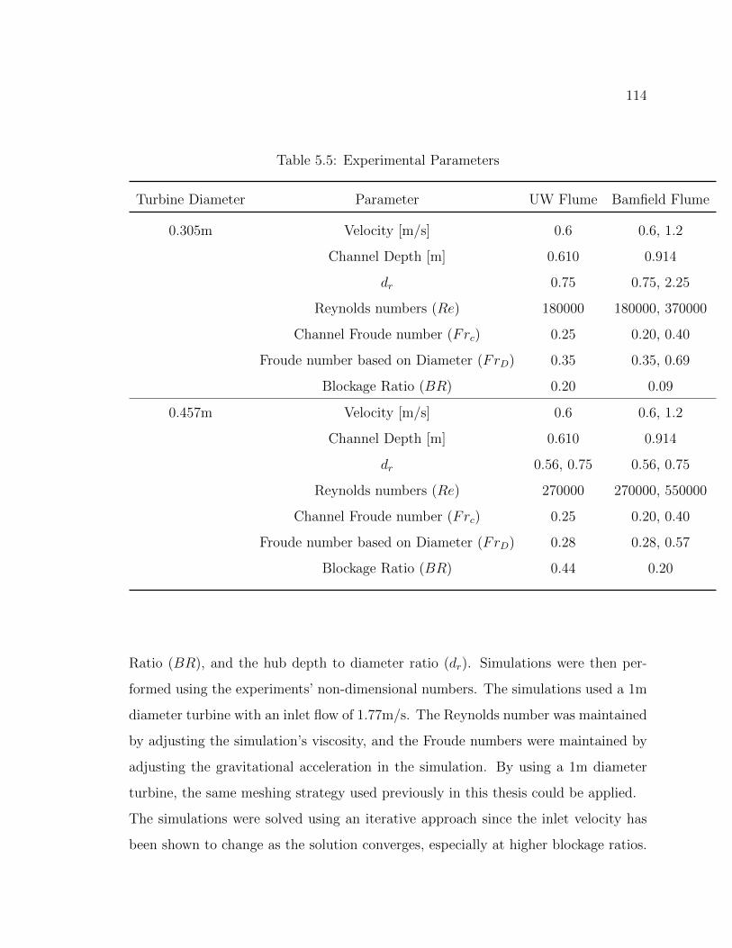
114
Table 5.5: Experimental Parameters
Turbine Diameter Parameter UW Flume Bamfield Flume
0.305m Velocity [m/s] 0.6 0.6, 1.2
Channel Depth [m] 0.610 0.914
dr 0.75 0.75, 2.25
Reynolds numbers (Re) 180000 180000, 370000
Channel Froude number (Frc) 0.25 0.20, 0.40
Froude number based on Diameter (FrD) 0.35 0.35, 0.69
Blockage Ratio (BR) 0.20 0.09
0.457m Velocity [m/s] 0.6 0.6, 1.2
Channel Depth [m] 0.610 0.914
dr 0.56, 0.75 0.56, 0.75
Reynolds numbers (Re) 270000 270000, 550000
Channel Froude number (Frc) 0.25 0.20, 0.40
Froude number based on Diameter (FrD) 0.28 0.28, 0.57
Blockage Ratio (BR) 0.44 0.20
Ratio (BR), and the hub depth to diameter ratio (dr). Simulations were then per-
formed using the experiments’ non-dimensional numbers. The simulations used a 1m
diameter turbine with an inlet flow of 1.77m/s. The Reynolds number was maintained
by adjusting the simulation’s viscosity, and the Froude numbers were maintained by
adjusting the gravitational acceleration in the simulation. By using a 1m diameter
turbine, the same meshing strategy used previously in this thesis could be applied.
The simulations were solved using an iterative approach since the inlet velocity has
been shown to change as the solution converges, especially at higher blockage ratios.

115
First, 1.77m/s was set as the inlet velocity magnitude, and the solution was allowed
to converge. The velocity magnitude supplied to the inlet was then increased by the
difference between 1.77m/s and the velocity at the inlet of the converged solution.
This was done until the converged inlet velocity was within ± 0.01m/s of 1.77m/s,
ensuring the turbine was operating at the desired TSR, Re, Frc and FrD. The
TSR used in each simulation was the TSR that provided the maximum Cp for the
simulation’s blockage ratio, see Figure 5.23.
5.5.3 Free Surface Fluctuation Results
Figure 5.27a shows the free surface fluctuations of three different simulations per-
formed with the same blockage ratio and the same non-dimensionalized depth. Each
simulation had different Froude numbers and a different Reynolds number. Since
the free stream velocity and the turbine diameter were the same in every simula-
tion, the Froude numbers and the Reynolds number were adjusted by changing the
simulation’s gravitational acceleration term and the simulation’s viscosity term. By
examining the equation for conservation of momentum for open channel flows with a
turbine, Equation 3.50, it can be seen that viscosity only affects the change in free
surface height related to the friction on the bottom of the channel. Therefore, the
change in height resulting from the energy extracted by the turbine is affected by the
gravitational acceleration term, and hence the Froude number. The difference in the
Froude number for each simulation is also responsible for the difference in stationary
waves downstream of the turbine.
In Section 5.2, Frc was proven to have a negligible effect on the free surface drop
across the turbine, whereas FrD was shown to have a substantial effect on the drop in
free surface elevation. The theoretical predictions for the change in free surface height
related to bottom friction and the force of the turbine on the flow are shown in Figure
5.27b. The simulations and the theoretical predictions have the same magnitude of
elevation change. This suggests that the simulations’ free surface behavior is realistic.
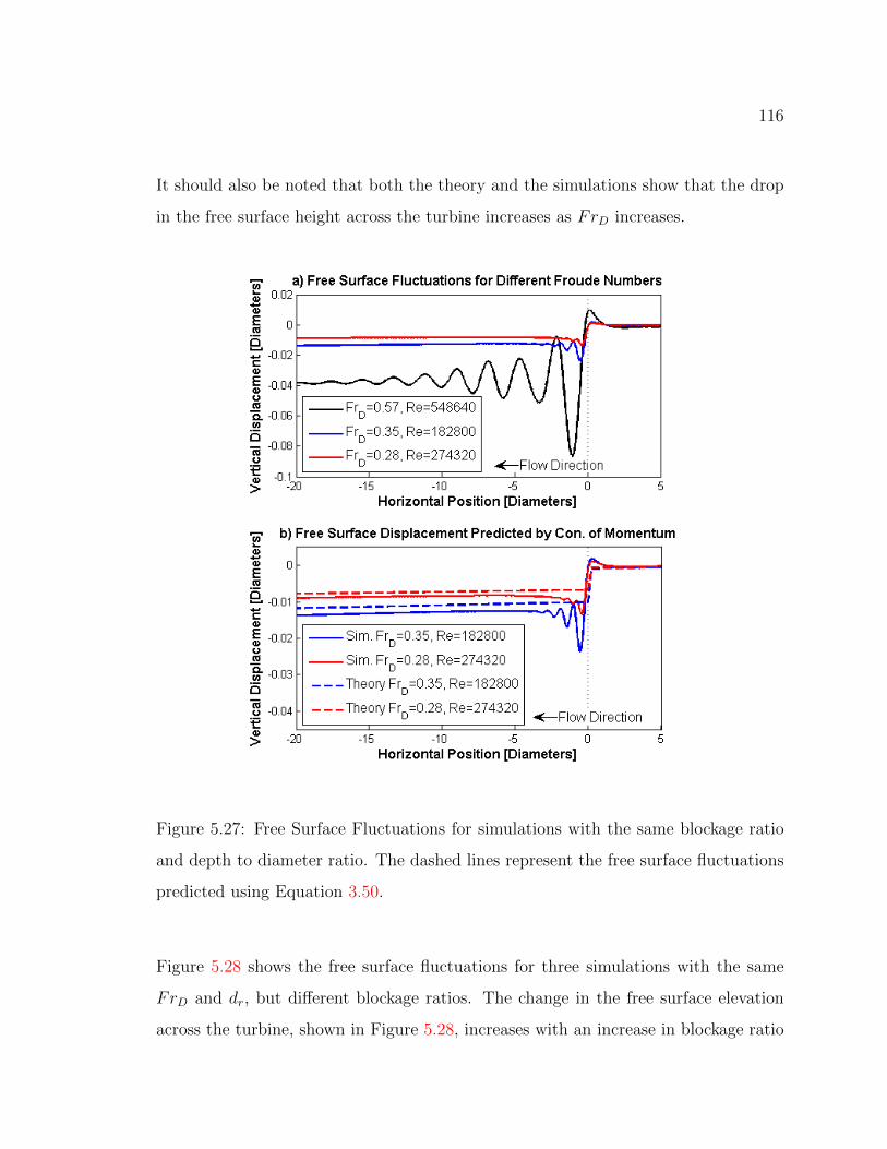
116
It should also be noted that both the theory and the simulations show that the drop
in the free surface height across the turbine increases as FrD increases.
Figure 5.27: Free Surface Fluctuations for simulations with the same blockage ratio
and depth to diameter ratio. The dashed lines represent the free surface fluctuations
predicted using Equation 3.50.
Figure 5.28 shows the free surface fluctuations for three simulations with the same
FrD and dr, but different blockage ratios. The change in the free surface elevation
across the turbine, shown in Figure 5.28, increases with an increase in blockage ratio

117
because more energy is extracted from the flow at higher blockage ratios.
The magnitude of the change in elevation across the turbine has been shown to depend
on FrD, as well as the blockage ratio. The relative importance of each variable to
the free surface elevation change can be seen by examining Figures 5.27 and 5.28. In
Figure 5.27 the free surface fluctuations for the same blockage ratio are shown, and
it can be seen that by doubling FrD the drop in free surface height quadruples. In
Figure 5.28 the free surface fluctuations for a constant FrD are shown, and it can be
seen that by doubling the blockage ratio the free surface drop approximately doubles.
Therefore, FrD has more of an effect on the free surface drop across the turbine than
the blockage ratio.
Figure 5.28: Free surface fluctuations for three simulations with the same Froude
number, based on turbine diameter (FrD = 0.35), and the same non-dimensional
turbine depth (dr = 0.75)

118
The free surface fluctuations near the turbine for simulations with a dr of 0.75 can be
seen in Figure 5.29. The positions of both the first standing wave and the deformation
in the free surface directly upstream of the turbine can be seen in Table 5.6. The
following are general conclusions based on these results (dr is held constant in these
results):
• The deformation of the free surface directly upstream of the turbine increases
with FrD.
• The horizontal location of the maximum height of the free surface deformation,
upstream of the turbine, moves closer to the turbine’s location as FrD increase.
• The depth of the standing wave downstream of the turbine increases with FrD.
• The horizontal position of the stationary wave moves further downstream from
the turbine as FrD is increased.
• The wavelength between the trough of the first two waves increases with an
increase in FrD.
The blockage ratio’s effects on the stationary waves can be seen by comparing the
simulations performed with a FrD of 0.35, see Figure 5.28. The free surface fluctua-
tions from the three cases look very similar because they have the same FrD and the
same dr. However, since the free surface fluctuations are not identical it is reasonable
to conclude that the blockage ratio also affects the free surface fluctuations near the
turbine. The blockage ratio appears to have the following effects on the stationary
waves downstream of the turbine:
• The first stationary wave increases in depth with the blockage ratio.
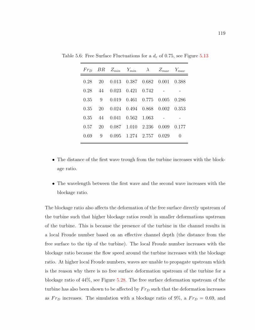
119
Table 5.6: Free Surface Fluctuations for a dr of 0.75, see Figure 5.13
FrD BR Zmin Ymin λ Zmax Ymax
0.28 20 0.013 0.387 0.682 0.001 0.388
0.28 44 0.023 0.421 0.742 - -
0.35 9 0.019 0.461 0.775 0.005 0.286
0.35 20 0.024 0.494 0.868 0.002 0.353
0.35 44 0.041 0.562 1.063 - -
0.57 20 0.087 1.010 2.236 0.009 0.177
0.69 9 0.095 1.274 2.757 0.029 0
• The distance of the first wave trough from the turbine increases with the block-
age ratio.
• The wavelength between the first wave and the second wave increases with the
blockage ratio.
The blockage ratio also affects the deformation of the free surface directly upstream of
the turbine such that higher blockage ratios result in smaller deformations upstream
of the turbine. This is because the presence of the turbine in the channel results in
a local Froude number based on an effective channel depth (the distance from the
free surface to the tip of the turbine). The local Froude number increases with the
blockage ratio because the flow speed around the turbine increases with the blockage
ratio. At higher local Froude numbers, waves are unable to propagate upstream which
is the reason why there is no free surface deformation upstream of the turbine for a
blockage ratio of 44%, see Figure 5.28. The free surface deformation upstream of the
turbine has also been shown to be affected by FrD such that the deformation increases
as FrD increases. The simulation with a blockage ratio of 9%, a FrD = 0.69, and
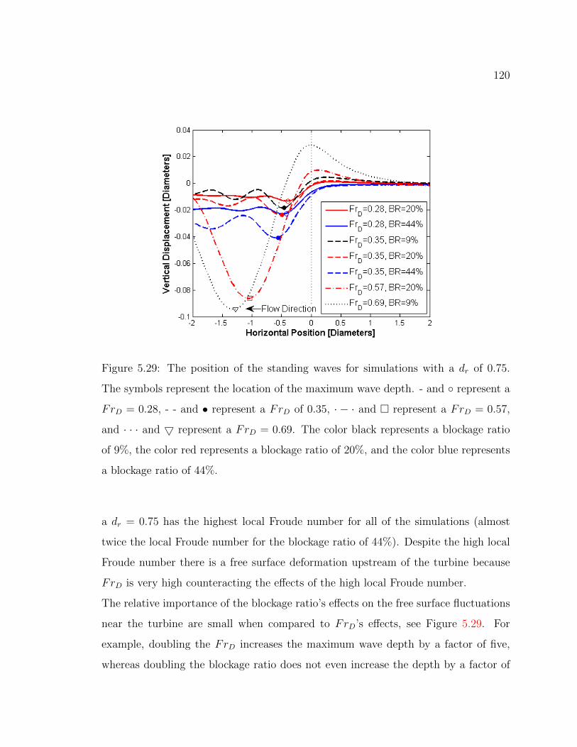
120
Figure 5.29: The position of the standing waves for simulations with a dr of 0.75.
The symbols represent the location of the maximum wave depth. - and ◦ represent a
FrD = 0.28, - - and • represent a FrD of 0.35, · − · and � represent a FrD = 0.57,
and · · · and 5 represent a FrD = 0.69. The color black represents a blockage ratio
of 9%, the color red represents a blockage ratio of 20%, and the color blue represents
a blockage ratio of 44%.
a dr = 0.75 has the highest local Froude number for all of the simulations (almost
twice the local Froude number for the blockage ratio of 44%). Despite the high local
Froude number there is a free surface deformation upstream of the turbine because
FrD is very high counteracting the effects of the high local Froude number.
The relative importance of the blockage ratio’s effects on the free surface fluctuations
near the turbine are small when compared to FrD’s effects, see Figure 5.29. For
example, doubling the FrD increases the maximum wave depth by a factor of five,
whereas doubling the blockage ratio does not even increase the depth by a factor of
121
two. Thus the FrD is more important to the free surface fluctuations near the turbine.
5.5.4 Coefficient of Power Results
Figures 5.30 and 5.31 show the Cp values for the different simulations performed in
this section. The conclusions described below have been reached using the data from
these figures, but it should be noted that the Cp may depend on multiple different
parameters (e.g. Blockage Ratio, TSR, FrD, dr, and Frc), thus analyzing the effects
of parameters graphically is difficult especially since there have been a limited number
of simulations preformed.
As predicted by theory, the coefficient of power increases with the increase in blockage
ratio [1] [3]. All of the simulations performed with a blockage ratio of 9% produce ap-
proximately the same Cp, which in some cases is slightly higher than the Cp produced
in the simulations without a free surface (the simulations used to obtain the TSR
vs. Cp curves were performed without a free surface to save computational time).
For the two simulations performed with a blockage ratio of 9% and a FrD = 0.69,
the one with a dr of 0.75 produced less power than the one with a dr of 2.25. One
possible explanation for the lower Cp value, is the increase in the free surface height
just upstream of the turbine that occurs when the turbine is in close proximity to
the free surface. This produces a larger cross sectional area near the turbine, which
slightly decreases the velocity at the turbine leading to less power produced. The
coefficients of power are calculated using the free stream velocity and do not account
for the slower speed seen at the turbine in the case with a dr of 0.75.
The coefficient of power is approximately the same for all simulations with a blockage
ratio of 9%, and for all simulations with a blockage ratio of 20%, leading to the
conclusion that for blockage ratios less than 20%, Cp is independent of FrD and Frc,
see Figure 5.30 and Figure 5.31. Several theories predict that at higher blockage ratios
Cp will increase with an increase in the channel Froude number [3]. Figure 5.31 does
not show an increase in Cp related to the channel Froude number, for simulations

122
Figure 5.30: Coefficient of power for different blockage ratios and Froude numbers
compared to TSR versus Cp curves. The color blue represents a dr of 0.75, the color
magenta represents a dr of 0.56, and the color red represents a dr of 2.25.
with a blockage ratio of 20%. However, for simulations performed with a blockage
ratio of 44%, the Cp does appear to increase with an increase in FrD (and Frc), as
predicted by the unidirectional flow theory. There are two potential reasons for the
simulations with a blockage ratio of 20% not aligning with the theory. First, the
free surface deformation upstream of the turbine affects Cp, and second, a change in
the free surface height at the inlet slightly changes the blockage ratio, and hence the
Cp. Neither of these reasons, however, are expected to have significant effects on the
power produced.
As FrD increases for a given blockage ratio, the deformation in the free surface directly
upstream of the turbine also increases. This results in an increase in the cross sectional
area of the flow at the turbine, decreasing the average velocity at the turbine. Since
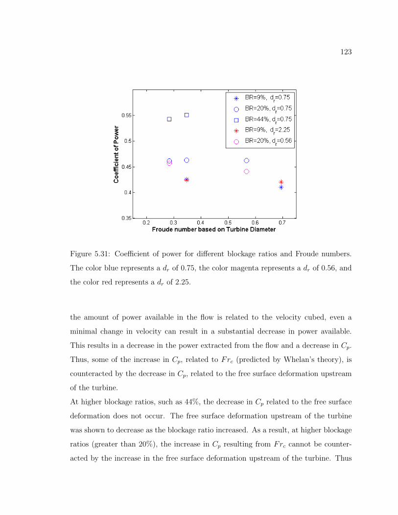
123
Figure 5.31: Coefficient of power for different blockage ratios and Froude numbers.
The color blue represents a dr of 0.75, the color magenta represents a dr of 0.56, and
the color red represents a dr of 2.25.
the amount of power available in the flow is related to the velocity cubed, even a
minimal change in velocity can result in a substantial decrease in power available.
This results in a decrease in the power extracted from the flow and a decrease in Cp.
Thus, some of the increase in Cp, related to Frc (predicted by Whelan’s theory), is
counteracted by the decrease in Cp, related to the free surface deformation upstream
of the turbine.
At higher blockage ratios, such as 44%, the decrease in Cp related to the free surface
deformation does not occur. The free surface deformation upstream of the turbine
was shown to decrease as the blockage ratio increased. As a result, at higher blockage
ratios (greater than 20%), the increase in Cp resulting from Frc cannot be counter-
acted by the increase in the free surface deformation upstream of the turbine. Thus
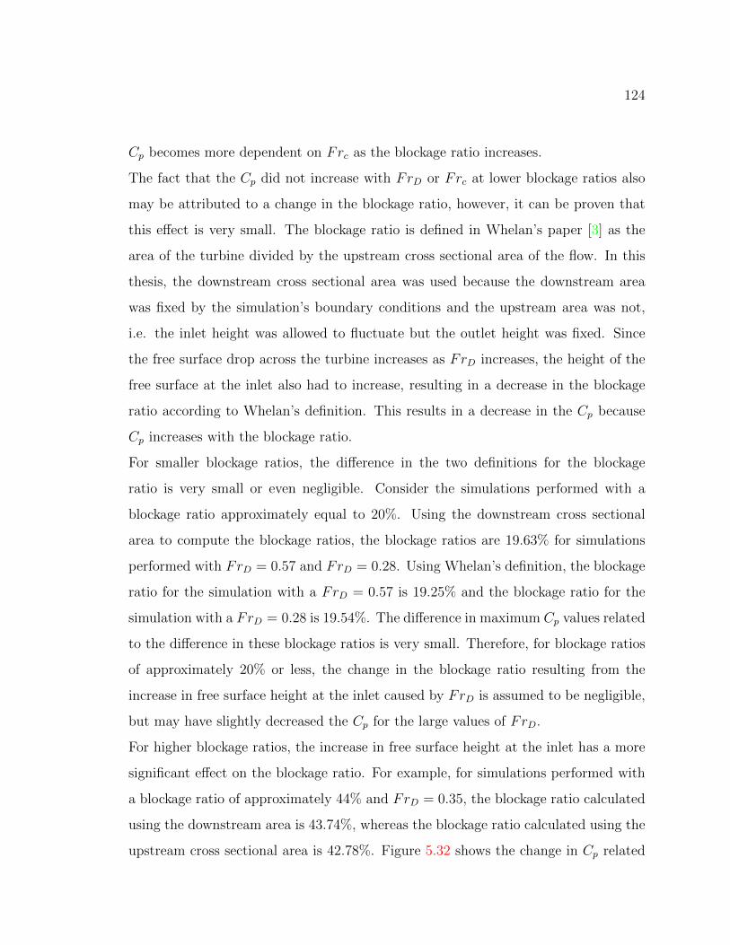
124
Cp becomes more dependent on Frc as the blockage ratio increases.
The fact that the Cp did not increase with FrD or Frc at lower blockage ratios also
may be attributed to a change in the blockage ratio, however, it can be proven that
this effect is very small. The blockage ratio is defined in Whelan’s paper [3] as the
area of the turbine divided by the upstream cross sectional area of the flow. In this
thesis, the downstream cross sectional area was used because the downstream area
was fixed by the simulation’s boundary conditions and the upstream area was not,
i.e. the inlet height was allowed to fluctuate but the outlet height was fixed. Since
the free surface drop across the turbine increases as FrD increases, the height of the
free surface at the inlet also had to increase, resulting in a decrease in the blockage
ratio according to Whelan’s definition. This results in a decrease in the Cp because
Cp increases with the blockage ratio.
For smaller blockage ratios, the difference in the two definitions for the blockage
ratio is very small or even negligible. Consider the simulations performed with a
blockage ratio approximately equal to 20%. Using the downstream cross sectional
area to compute the blockage ratios, the blockage ratios are 19.63% for simulations
performed with FrD = 0.57 and FrD = 0.28. Using Whelan’s definition, the blockage
ratio for the simulation with a FrD = 0.57 is 19.25% and the blockage ratio for the
simulation with a FrD = 0.28 is 19.54%. The difference in maximum Cp values related
to the difference in these blockage ratios is very small. Therefore, for blockage ratios
of approximately 20% or less, the change in the blockage ratio resulting from the
increase in free surface height at the inlet caused by FrD is assumed to be negligible,
but may have slightly decreased the Cp for the large values of FrD.
For higher blockage ratios, the increase in free surface height at the inlet has a more
significant effect on the blockage ratio. For example, for simulations performed with
a blockage ratio of approximately 44% and FrD = 0.35, the blockage ratio calculated
using the downstream area is 43.74%, whereas the blockage ratio calculated using the
upstream cross sectional area is 42.78%. Figure 5.32 shows the change in Cp related
125
to changing the blockage ratio from 43.74% to 42.78%, in simulations without a
free surface. The difference in blockage ratio produced a measurable but insignificant
difference in Cp. Figure 5.30 shows that for blockage ratios of 44% the Cp values found
in simulations with a free surface are less than simulations without a free surface (the
TSR versus Cp curve). The change in the blockage ratio caused by the increase in
inlet height is partially responsible for this difference.
The other reason the Cp is lower than the TSR versus Cp curve is that the curve was
created with the turbine centered in the channel (the hub was approximately 0.67D
away from the channel bottom), whereas to obtain a dr = 0.75 in the simulations with
a free surface the turbine had to be moved closer to the channel floor (the hub was
approximately 0.59D away from the channel floor). The no slip boundary condition
applied to the channel bottom causes a velocity gradient in the lower portion of the
channel. As a result, since the turbine was closer to the bottom in the simulations
with a free surface, the flow speeds through the turbine were lower, so the power
produced and the Cp values were lower, see Figure 5.32.
The velocity profile near the bottom of the channel is affected by the Reynolds number.
This results in turbines at the same hub depth being exposed to different velocities
depending on the Reynolds number. Thus, for turbines in close proximity to the
bottom of the channel, the Cp is also affected by the Reynolds number, which is
part of the reason why the simulation with FrD = 0.35 has a higher Cp than the
simulation with FrD = 0.28. Figure 5.32 shows for a constant blockage ratio and a
constant turbine depth, Cp changes depending on the Reynolds number.
Figure 5.33 shows the Cp values predicted by Whelan’s theory [3] for the different
experiments in Table 5.5, as well as the Cp values predicted by Garrett’s theory [1].
The increase in Cp related to the blockage ratio can be seen in both of the theories and
the numerical simulation results. However, the magnitude of Cp and the amount Cp
increases due to blockage ratio is substantially smaller for the numerical simulations.
At higher blockage ratios, like 44%, the simulations showed that the Cp increased

126
Figure 5.32: Coefficient of power for different blockage ratios. Symbols shaded green
represent simulations with a free surface, symbols shaded white represent simulations
without a free surface, the color black represents a non-dimensional hub depth (dr)
of 0.75D, and the color red represents a non-dimensional hub depth (dr) of 0.67D.
with Frc as predicted by theory, but not to the extent predicted.
One of the reasons the Cp from the simulations does not match the Cp predicted by
Garrett’s and Whelan’s theory is the turbines in the theory are operating with a dif-
ferent axial induction factor than the turbines in the simulations. The theoretical Cp
values shown in Figure 5.33 were computed using the optimum axial induction factor.
The optimum axial induction factor is the axial induction factor that corresponds to
the maximum possible coefficient of power. For a turbine operating in a channel with
a blockage ratio of 0, the optimum axial induction factor is 1/3 with Cp equaling
the Betz’s limit. Figure 2.1 shows that as the blockage ratio increases the optimum
axial induction factor also increases. Figure 5.34 shows the axial induction factor of
127
Figure 5.33: Coefficient of power for different blockage ratios and channel Froude
numbers. The color black represents the Cp from the numerical simulations. The color
red represents the Cp predicted by Whelan’s Theory [3]. The dashed line represents
the Cp calculated using Garrett’s Theory [1]. ◦ represents the Betz limit.
the turbines in the simulations and their respective Cp values. It is obvious that the
simulations are not operating at the optimum axial induction factor for their specific
blockage ratios because all of the axial induction factors are less than 0.2. In fact, for
the simulations, the axial induction factor decreased as the blockage ratios increased.
This is because at high blockage ratios there is less area around the turbine for flow
to be diverted leading to a larger flow rate through the turbine and a lower axial
induction factor.
Figure 5.34 shows the axial induction factor versus Cp curves predicted by Whelan’s
theory. By comparing the theory’s predicted values for Cp at the axial induction
factors found for the turbines in this thesis’s simulations, instead of the optimum

128
Figure 5.34: Coefficient of power versus axial induction factor for different blockage
ratios with a FrD = 0.35 and dr = 0.75.
axial induction factors, it can be seen that the simulations’ Cp values are about 70%
of the value predicted using Whelan’s theory. When Whelan compared the theory to
two sets of experiments, the experimental Cp values were about 60% of the Cp values
predicted by theory [3]. Therefore it appears that the simulations of this thesis are
producing reasonable results.
For a blockage ratio of 44%, the numerical simulation’s Cp values were only 60% of
the theoretical Cp values. One issue that maybe enhancing the difference between
simulated and theoretical Cp values at high blockage ratios is the theory assumes
subcritical flow [26]. The simulations show that for the blockage ratio of 44%, the
flow is supercritical near the turbine, so the theory may not be accurately representing
the flow, leading to inaccurate predictions of Cp. Furthermore, the theory is developed
assuming the flow is only in the streamwise direction, but at high blockage ratios the

129
flow becomes more three-dimensional deviating from the assumptions of the theory.
These issues explain the larger difference in Cp values for the blockage ratio of 44%.
The maximum Cp values predicted by Garrett’s and Whelan’s theory for the optimum
axial induction factor are significantly higher than the Cp values found in the numeri-
cal simulations, see Figure 5.33. The simulations were performed using the TSR that
produced the maximum coefficient of power because the TSR is one of the operating
parameter used by real turbines to adjust power, not the axial induction factor. By
changing the blade’s pitch and twist, the optimal TSR can be increased helping MHK
turbines to reach higher axial induction factors and possibly increase their maximum
Cp values. Furthermore, increasing the number of turbine blades can help increase the
axial induction factor of the turbine such that it could have a higher maximum Cp.
However, both of these suggestions involve designing turbines specifically for certain
flows instead of designing a turbine that can be applied universally.
It is important to understand that real turbines typically do not operate with the
ideal parameters used by theory to predict the maximum Cp, so real turbines will not
produce the same Cp. Therefore, caution must be used when applying theory because
it can significantly over predict Cp when unrealistic, yet ideal, conditions are used,
giving a false understanding of the amount of power that can be produced in reality.

130
Chapter 6
SUMMARY, CONCLUSIONS, AND FUTURE WORK
MHK turbines are a promising new technology for energy production that relies on
converting energy from tidal currents into electricity. Wind turbines and MHK tur-
bines have numerous similarities and as such many of the same models and theories
that have been applied for decades to wind energy can now be applied to tidal energy.
However, there are a few key differences between wind energy and tidal energy that
can affect the operating characteristics of a turbine. This thesis specifically examines
one of these key differences: the effect of the presence of a free surface on the oper-
ating characteristics of a horizontal axis MHK turbine. Associated with the presence
of a free surface, although independent from it, is the concept of blockage ratio: the
ratio of cross sectional area swept by the turbine rotor to the total cross sectional
area in the channel; this is another key parameter for MHK turbines that is studied
in depth in this thesis.
The presence of a free surface creates higher blockage ratios for MHK turbines than
for wind turbines. In many cases this negates the application of the Betz limit because
the Betz limit assumes negligible blockage ratio. According to theoretical analyses
performed by Garrett [1], Whelan [3], and Polagye [26] increasing the blockage ratio
increases the maximum possible coefficient of power for a turbine. These are simple
one-dimensional models, therefore, it is important to determine, from fully three
dimensional turbulent flow with a realistic representation of the MHK turbine, the
extend of the effect that blockage ratio has on the power produced by a turbine.
Another effect the free surface has on MHK turbines is it constrains the turbine’s
wake expansion creating an asymmetric wake. Since in turbine arrays the wake of
131
one turbine is the inflow conditions for another turbine it is important to understand
the affects of the free surface on the wake, to ensure optimal turbine array designs.
6.1 Summary of Numerical Methodology
The computational simulation of MHK turbines in an open channel requires a num-
ber of sophisticated models for the turbulent flow, the turbine implementation and
the tracking of the free surface. Additionally, it is important to carefully construct
the computational mesh to treat every aspect of the simulation with accuracy and
stability. Finally, the selection of adequate boundary conditions is not trivial and can
significantly affect the results.
In the simulations included in this thesis that study the flow around an MHK turbine
in the presence of a free surface, the mesh had to be refined near the air-water interface
in order to capture the free surface height and fluctuations. The mesh also had to be
refined in the wake region to ensure the evolution of the wake was properly modeled.
An unstructured mesh was used to transition from critical regions in the domain,
where a fine mesh was necessary, to regions with low gradients, near the inlet and
towards the sides and outlet of the domain, where a coarse mesh was acceptable, in
order to minimize the number of mesh elements.
The Virtual Blade Model (VBM) was used in the numerical simulations to implement
the presence of the turbine rotor blades in the equations of motion. VBM was selected
because it models the time-averaged aerodynamic effect of rotating blades using values
for the coefficients of lift and drag developed by a higher accuracy model, while
not requiring the blade geometry to be meshed. This saves computational time,
because VBM requires less mesh elements than moving reference frame or moving
mesh simulations that model the actual blade geometry, and the solution is steady
state since the effect of the blades is time-averaged.
The Volume of Fluid (VOF) model was used in the numerical simulations to model
the two fluids, water and air, and to track the free surface. VOF was used because

132
it is less computationally expensive than other multiphase models and more stable in
cases that do not require a sharp interface to be tracked. VOF requires the solution
of a continuity equation for each fluid and a single momentum equation. A series
of simulations were performed to determine the correct boundary conditions to use
in this problem. Results from different boundary conditions (mass flow rate, fixed
pressure, fixed free surface height) at the inlet and outlet were compared to the free
surface profile predicted by theory. Typical boundary conditions were applied at the
channel side walls: no slip for the bottom, symmetry for the top and sides. Pressure
Inlet with the Open Channel Flow Option for the inlet, and Pressure Outlet with the
Open Channel Flow Option for the outlet produced the most accurate free surface
profile and was used in all the numerical simulations in this thesis. The pressure
specification method applied to the outlet was a user-prescribed free surface height
and bottom height.
6.2 Summary of the Interactions Between the Free Surface and a Hor-izontal Axis Turbine at Low Blockage Ratios
When a turbine is in close proximity to the free surface, the wake will expand to
interact with the surface. It was previously believed [18] that the wake of a turbine
close to the free surface will recover in a shorter distance than the wake of a turbine
far away from the free surface. This incorrect statement was arrived at by examining
the downstream centerline velocity measurements. However, the velocity minimum
in the wake of a turbine close to the free surface does not occur at the turbine’s
centerline. By examining the minimum velocity in the turbine’s wake, we found that
the wake actually recovers slower for turbines close to the free surface. The recovery
is slower because the wake is not exposed to the same mixing with high momentum
fluid and the current’s high momentum fluid surrounding the wake is responsible for
wake recovery.
It was also observed that the total drop in free surface height across a channel re-
133
mained constant for simulations performed in the same channel with the same turbine,
regardless of the turbine’s vertical position. This was because the power extracted
by the turbine and the friction factor were independent of the vertical position of the
turbine. The free surface fluctuations near the location of the turbine rotor, however,
did depend strongly on the depth of the turbine.
6.3 Summary of the Non-Dimensional Numbers used to Characterizethe Effects of a MHK Turbine on the Free Surface
The Froude number is the non-dimensional number most often used to analyze flows
with a free surface. For open channel flows without a MHK turbine the characteristic
length scale used in the Froude number is the channel depth. By comparing the free
surface fluctuations from simulations with different channel depths (and associated
different channel Froude number values), it was concluded that the free surface fluc-
tuations do not depend on channel depth, for values of Fr below 0.5 and blockage
ratios below 0.2. Therefore, for open channel flows with a MHK turbine, the channel
Froude number is irrelevant to the flow and the MHK turbine performance for re-
alistic values away from the most extreme conditions for shallow channel depth and
blockage ratios.
Several other length scales were examined as critical parameters for controlling the
behavior of the flow. Two relevant length scales are the turbine’s tip depth and the
turbine’s hub depth. Neither length scale provided the a complete characterization
of the free surface fluctuations (through the depth-based Froude number) because
neither scale accounted for the size of the turbine. The turbine diameter was then
applied as the length scale, but the free surface fluctuation appeared to also depend
on the turbine’s depth. The application of two non-dimensional numbers was the
solution. One non-dimensional number was the Froude number with a characteristic
length of the turbine diameter (FrD), and the other was a non-dimensional depth
equal to the hub depth divided by the turbine diameter (dr). When simulations had
134
the same Froude number based on turbine diameter and the same depth ratio, the
free surface shape downstream of the turbine was identical.
The free surface waves may affect objects downstream of the turbine so it is important
to understand how waves respond to changes in the flow non-dimensional parameters:
waves increased in magnitude as FrD increased and as dr decreased; the distance
downstream to the first wave trough (wavelength) increased with increases in FrD
but decreased with increases in dr.
6.4 Summary of the Effects of the Free Surface on the Coefficient ofPower at Low Blockage Ratios
The coefficient of power (Cp) at low blockage ratios was not affected by the vertical
position of the turbine or by the channel depth. The wake resolution, however, affected
the power extracted by the turbine so it was important to use an adequate mesh in
the turbine wake when comparing different size turbines. Special care was taken to
use the same size mesh cells near the free surface regardless of the turbine diameter
because the resolution of the free surface fluctuations required sufficient resolution in
the mesh near the free surface.
6.5 Summary of the Blockage Ratio Effects on MHK Turbine Perfor-mance
Preliminary simulations performed at different blockage ratios showed Cp increased
with the blockage ratio. It was also proven that as the blockage ratio increased the
value of TSR ratio for optimum Cp increased. Higher blockage ratios lead to a higher
velocity through the turbine, which decreases the actual TSR subsequently decreasing
Cp since Cp is related to the actual TSR. The actual TSR is the TSR based on the
velocity at the turbine rotor plane (rather than based on the free stream velocity as
it is usually defined). New TSR versus CP curves were created to determine the TSR
based on the free stream velocity that produced the maximum Cp for each blockage

135
ratio. The free stream velocity was used to calculate the TSR-case-label because it is
known prior to the performance of the simulation.
6.6 Summary of the Numerical Simulations of Experiments Performedwith Scaled Turbines
A set of simulations were performed to model experiments of scaled MHK turbines.
The experiments will be performed using two different flumes to provide different
blockage ratios. The simulations will be compared against the experimental data, to
provide experimental validation for the conclusions of this thesis.
The simulations were performed using a 1m diameter turbine used in the other sim-
ulations of this thesis. This allowed us to leverage the computational simulation
effort developed in the first part of the thesis, without the need to repeat the mesh
creation for different domains. All the simulations were performed matching the non-
dimensional numbers in the experiments. The gravitational acceleration and the fluid
viscosity were changed to explore the relevant range of non-dimensional parameters
with the different simulations.
The drop in the free surface height across the turbine was determined to be related
to the blockage ratio as well as the Turbine Froude number (FrD). If either the
blockage ratio or FrD was increased, the drop in free surface height across the turbine
would increase but for different reasons. At higher blockage ratios the drop increased
because more power was extracted from the flow, whereas, an increase in FrD lowered
the effective gravity (lowering gravity is equivalent to increasing the FrD since all
simulations were performed with the same diameter turbine at the same flow speed)
which increased the elevation change across the turbine as predicted by theory.
The free surface waves downstream of the turbine were also shown to be affected by
the blockage ratio and FrD. For larger blockage ratios the first wave trough moved
further downstream from the turbine and the wave depth increased. The effects
of FrD on the surface waves, found for low blockage ratios, were verified at higher

136
blockage ratios: increasing FrD increased the wave depth, the wave length, and the
distance downstream where the first wave trough occurred.
The free surface deformation upstream of the turbine was shown to be dependent on
FrD, dr and the blockage ratio. The deformation increased for larger turbine rotor
diameter (FrD), and decreased with an increase in blockage ratio and turbine depth
(dr). The free surface deformation decreased with blockage ratio because at higher
blockage ratios there is less area around the turbine for the flow to be diverted resulting
in a higher velocity around the turbine than that seen at low blockage ratios. When
high blockage ratio values, such as 44%, the flow near the turbine becomes locally
supercritical and free surface gravity waves cannot travel upstream of the turbine.
Thus, the free surface upstream of the turbine is not deformed.
The rise in the free surface directly upstream of the turbine related to FrD and dr had
a small effect on the power extraction (Cp). The free surface deformation resulted in
a larger cross sectional area of the flow at the turbine which slightly decreased the
velocity through the turbine. Since the power available in the flow is proportional to
the velocity cubed, even a slight change in the velocity at the rotor disk can result
in a appreciable change in the power extracted. Therefore, less power was extracted
from flows with a large free surface rise just upstream of the turbine.
Several papers have suggested that, at high blockage ratios, increasing the channel
Froude number (Frc) will increase Cp. The results of this thesis, however, do not
support that conclusion for blockage ratios less than 20%. Any increase in Cp related
to an increase in Frc was counteracted by the decrease in Cp related to the rise in
the free surface directly upstream of the turbine. At higher blockage ratios, such as
44%, there was no deformation upstream of the turbine so Cp did increase slightly
with Frc. However, the increase in Cp due to Frc was much less pronounced than
predicted by theory.
137
6.7 General Conclusions
The purpose of this thesis was to determine under which conditions it is necessary
to include the free surface in numerical simulations of MHK turbines. There are
generally two reasons for simulating MHK turbines: one is to examine the turbine’s
wake and the second is to examine the coefficient of power. Since the presence of a
free surface affects each differently, the analysis of the free surface in MHK turbine
simulations will be discussed based on the goal of the simulation.
The free surface was shown to affect the wake evolution downstream of the turbine
when the turbine had a hub depth to diameter ratio of less than 1.5. Therefore, if the
wake characteristics are the focus of a study, such as for array optimization, including
the free surface in the numerical simulations will improve the physical representation
of the flow and the validity of the results. This will ensure more realistic inflow
conditions for downstream turbines in the array. The free surface fluctuations may
also play an important role in turbine array design. As FrD is increased or dr is
decreased, the depth of the free surface waves downstream of the turbines increases.
The wave depth increased to as much as 0.1 rotor diameters for the case of FrD = 0.69
and dr = 0.75. Since the waves extend downstream of the turbine, any turbine placed
downstream of the first rows of turbines in an array may experience the effects of the
free surface fluctuations. This could affect the downstream turbine’s wake as well as
it’s coefficient of power and increase the variable loading on the downstream turbines.
Therefore, when studying turbine arrays where the turbines are in close proximity to
the free surface, the free surface should be included in the simulations.
For single turbines (not in an array), the coefficient of power for blockage ratios of
20% or less have been shown to be independent of or negligibly dependent on FrD,
Frc, and dr. For blockage ratios greater than 20% the coefficient of power was shown
to vary only slightly with the channel Froude number, and the increase in Cp may be
neglected in most cases.

138
The coefficient of power was shown to be heavily dependent on the blockage ratio.
Therefore, when simulations are performed to study the coefficient of power, it is not
necessary to include the free surface as long as the simulations are performed with
the correct blockage ratio. The only exception to this conclusion is for turbines used
to hydraulically control a channel, because the range of blockage ratios and Froude
numbers used in those cases are very extreme, and outside the conditions studied in
this thesis [55].
Performing simulations without a free surface represent significantly reduced compu-
tational requirements. Simulations without a free surface require less mesh elements,
converge at lower number of iterations, and the inlet boundary condition’s are easier
to establish. Thus, simulations without a free surface have a much shorter compu-
tational time, require less memory allocation and less operator time in meshing and
setting up the simulations. A simulation was performed with and without a free
surface to determine the computational expense of including a free surface. The sim-
ulation with a free surface took nine times longer to converge than the simulation
without the free surface. Therefore, simulations should only be performed with a free
surface when it is essential to closely represent the free surface effects in the problem
under study, such as when information is required about the details of the wake or
when the free surface height may affect other turbines or topography in the vicinity.
6.8 Future Work
The numerical simulations of MHK turbine experiments must be validated using
experimental data, to ensure the coefficient of power as well as free surface fluctua-
tions found numerically are accurate. Once the simulations are validated, the same
methodology used in this thesis can be applied to the study of an array of horizontal
axis turbines in order to determine if the free surface fluctuations from an upstream
turbine will significantly affect the operating characteristics of downstream turbines.
For any continuing research on the free surface effects on MHK turbines at high

139
blockage ratios it would be beneficial to develop a new set of boundary conditions.
The new inlet boundary condition should allow the user to fix the inlet velocity of
the water and fix the inlet free surface height. Since the inlet height is fixed, the
new outlet boundary condition must allow the outlet height to fluctuate, in order to
account for the energy extracted by the turbine and the energy loss due to the friction
on the bottom of the channel. New boundary conditions similar to these will ensure
the numerical model is describing the desired flow, i.e. has the correct inlet velocity
and the correct blockage ratio.
140
BIBLIOGRAPHY
[1] C. Garrett and P. Cummins. The efficiency of a turbine in a tidal channel. J.
Fluid Mechanics, 588:243–251, 2007.
[2] M. R. Ruith. Unstructured, multiplex rotor source model with thrust and mo-
ment trimming- fluent’s vbm model. Technical report, Fluent Inc., 2005.
[3] J. I. Whelan, J. M. R. Graham, and J. Perio. A free-surface and blockage cor-
rection for tidal turbines. J. Fluid Mechanics, 624:281–291, 2009.
[4] 2009 energy enpenditure per person, 2012. URL http://energy.gov/maps/
2009-energy-expenditure-person.
[5] United States Census Bureau. The 2012 statistical abstract: Energy and utilities,
2012. URL http://www.census.gov/prod/2011pubs/12statab/energy.pdf.
[6] Energy Information Administration. Annual energy review 2011, September 2012
2012. URL http://www.eia.gov/totalenergy/data/annual/pdf/aer.pdf.
[7] S. E. Ben Elghali, M. E. H. Bendouzid, and J. F. Charpentier. Marine tidal
current electric power generation technology: State of the art and current status.
Electric Machines & Drives Conference, 2:1407–1412, 2007.
[8] B. Polagye, B. Van Cleve, A. Copping, and K. Kirkendall, editors. Environmental
Effects of Tidal Energy Development, number NMFS F/SPO-116, 186 p. in U.S.
Dept. Commerce, NOAA Tech. Memo., 2010.
[9] T. J. Hall. Numerical simulation of a cross flow marine hydrokinetic turbine.
Master’s thesis, University of Washington, 2012.
141
[10] G. Hagerman, B. Polagye, R. Bedard, and M. Previsic. Methodology for estimat-
ing tidal current energy resources and power production by tidal in-stream energy
conversion (tisec) devices. Technical report, Electric Power Research Institute
Inc. (EPRI), 2006.
[11] I. G Bryden, S. J Couch, A. Owen, and G. Melville. Tidal current resource assess-
ment. Proceedings of the Institution of Mechanical Engineers. Part A, Journal
of Power and Energy, 221:125–135, 2007.
[12] S. Antheaume, T. Maitre, and J. Achard. Hydraulic darrieus turbines effieciency
for free fluid flow conditions versus power farms conditions. Renewable Energy,
33:2186–2198, 2008.
[13] Marine current turbines. URL http://www.marineturbines.com/.
[14] F. O Rourke, F. Boyle, and A. Reynolds. Tidal energy update 2009. Applied
Energy, 87:398–409, 2010.
[15] Open hydro tidal technology. URL http://www.openhydro.com/company.html.
[16] Andritz hydro hammerfest. URL http://www.hammerfeststrom.com/.
[17] Ocean renewable power company. URL http://www.orpc.co/default.aspx.
[18] X. Sun. Numerical and Experimental Investigation of Tidal Current Energy Ex-
traction. PhD thesis, The University of Edinburgh, 2008.
[19] X. Sun, J. P. Chick, and I. G. Bryden. Laboratory-scale simulation of energy
extraction from tidal currents. Renewable Energy, 33:1267–1274, 2008.
[20] F. M. White. Fluid Mechanics. McGraw-Hill, 7th edition, 2011.

142
[21] L. E. Myers, A. S. Bahaj, R. I. Rawlinson-Smith, and Thomson M. The effect
of boundary proximity upon the wake structure of horizontal axis marine cur-
rent turbines. In Proceeding of the 27th International Conference on Offshore
Mechanics and Artic Engineering, 2008.
[22] A. S. Bahaj, L. E. Myers, R. I. Rawlinson-Smith, and M. Thomson. The effects
of boundary proximity upon the wake structure of horizontal axis marine current
turbines. Journal of Offshore Mechanics and Arctic Engineering, 134:021104:1–8,
2012.
[23] L. E. Myers and A. S. Bahaj. Experimental analysis of the flow field around
horizontal axis tidal turbines by use of scale mesh disk rotor simulators. Ocean
Engineering, 37:218–227, 2010.
[24] A. Betz. Das maximum der theoretisch moglichen ausnutzung des wiwind durch
windmortoren. Z. Gesante Turbinenwesen, 26:307–309, 1920.
[25] T. Burton, D. Sharpe, N. Jenkins, and E. Bossanyi. Wind Energy Handbook.
John Wiley & Sons, Ltd, 2001.
[26] B. Polagye. Hydrodynamic Effects of Kinetic Power Extraction by In-Stream
Tidal Turbines. PhD thesis, University of Washington, 2009.
[27] T Javaherchi. Numerical modeling of tidal turbines: Methodology development
and potential physical environmental effects. Master’s thesis, University of Wash-
ington, 2010.
[28] M. E. Harrison, W. M. J. Batten, L. E. Myers, and A. S. Bahaj. A comparison
between cfd simulations and experiments for predicting the far wake of horizontal
axis tidal turbine. In Proceeding of the 8th European Wave and Tidal Energy
Conference, 2009.

143
[29] M. E. Harrison, W. M. J. Batten, L. E. Myers, and A. S. Bahaj. Comparison
between cfd simulations and experiments for predicting the far wake of horizontal
axis tidal turbines. IET Renewable Power Generation, 4-6:613–627, 2010.
[30] ANSYS FLUENT 14.0 User’s Guide, Chapter 7 Cell Zone and Boundary Con-
ditions, Section 7.2.3, Porous Media Conditions and Section 7.3.2. Using Flow
Boundary Conditions, 2011.
[31] A. S. Bahaj, W. M. J. Batten, and G. McCann. Experimental verifications
of numberical predictions for the hydrodynamic performance of horizontal axis
marine current turbines. Renewable Energy, 32:2479–2490, 2007.
[32] S. R. Turnock, A. B. Phillips, J. Banks, and R. Nicholls-Lee. Modelling tidal
current turbine wakes using a coupled rans-bemt approach as a tool for analysing
power capture of arrays of turbines. Ocean Engineering, 38:1300–1307, 2011.
[33] W. M. J. Batten, A. S. Bahaj, A. F. Molland, and J. R. Chaplin. Experimental
validated numerical method for the hydrodynamic design of horizontal axis tidal
turbines. Ocean Engineering, 34:1013–1020, 2007.
[34] A. S. Bahaj, A. F. Molland, J. R. Chaplin, and W. M. J. Batten. Power and
thrust measurements of marine current turbines under various hydrodynamic
flow conditions in a cavitation tunnel and a towing tank. Renewable Energy, 32:
407–426, 2007.
[35] A. S. Bahaj, Thomson M. Myers, L. E., and N. Jorge. Characterising the wake
of horizontal axis marine current turbines. In Proceedings of the 7th European
Wave and Tidal Energy Conference Porto, Portugal, 2007.
[36] A. J. Macleod, S. Barnes, K. G. Rados, and I. G. Bryden. Wake effects in
tidal current farms. In Proceedings of the international conference on marine
renewable energy, Newcastle upon Tyne, UK, 2002.

144
[37] C. A. Consul, H. J. Wilden, and S. C. McIntosh. Blockage effects on the hydro-
dynamic performance of a marine cross-flow turbine. Philosophical Transactions
of the Royal Society A, 371:1–16, 2013.
[38] H. K. Versteeg and W Malalasekera. An Introduction to Computational Fluid
Dynamics- The Finite Volume Method. Pearson Education Limited, 2007.
[39] S. B. Pope. Turbulent Flows. Cambridge University Press, 2000.
[40] A. Gosset and G. Flouriot. Optimization of power extraction in an array of
marine hydrokinetic turbines. Technical report, French Naval Academy, 2008.
[41] ANSYS FLUENT Theory Guide Release 14.0, Chapter 17, Section 17.3, Novem-
ber 2011.
[42] C. W. Hirt and B. D. Nichols. Volume of fluid (vof) method for the dynamics of
free boundaries. Journal of Computational Physics, 39:201–225, 1981.
[43] ANSYS FLUENT 14.0 User’s Guide, Chapter 26, Modeling Multiphase Flows,
2011.
[44] M. J. Lawson, Y. Li, and D. C. Sale. Development and verification of a com-
putational fluid dynamics model of a horizontal-axis tidal current turbine. In
Proceedings of the 30th International Conference on Ocean, Offshore and Arctic
Engineering, 2011.
[45] M. Tessier and N. Tomasini. Numerical study of horizontal axis hydrokinetic
turbines: Performance analysis and array optimization. Technical report, French
Naval Academy in Collaboration with University of Washington, 2012.
[46] ANSYS FLUENT Theory Guide Release 14.0, Chapter 4, Turbulence, November
2011.
145
[47] J. Thomson, B. Polagye, V. Durgesh, and M. Richmond. Measurements of tur-
bulence at two tidal energy sites in puget sound, wa. IEEE Journal of Oceanic
Engineering, 37:363–374, 2012.
[48] ANSYS FLUENT 14.0 User’s Guide, Chapter 29, Modeling Using the Solver,
2011.
[49] K. A. Haas, H. M. Fritz, S. P. French, B. T. Smith, and V. Neary. Assessment
of energy production potential from tidal streams in the united states. Technical
report, Georgia Tech Research Corporation, 2011.
[50] News lincoln county: Toledo man resues woman from car after it plunged
into yaquina river off highway 20, December 2012. URL http://www.
newslincolncounty.com/?cat=63.
[51] Q. Zhu, Y. Liu, and D. K. P. Yue. Numerical investigation of free-surface signa-
tures generated by submerged objects. 2006.
[52] P. K Kundu and I. M. Cohen. Fluid Mechanics. Academic Press, 2008.
[53] J. I. Whelan and T. Stallard. Arguments for modifying the geometry of a scale
model rotor. In 9th European Wave and Tidal Energy Conference, 2011.
[54] E. J. Schroeder. Low reynolds number flow validation using computational fluid
dynamcis with application to micro air vehcles. Master’s thesis, University of
Maryland, 2005.
[55] A. Hoseyni Chime. Analysis of hydrokinetic turbines in open channel flows.
Master’s thesis, University of Washington, 2013.
[56] Energy Information Administration. Greenhouse gases, climate change, and en-
ergy, April 2004. URL http://www.eia.gov/oiaf/1605/ggccebro/chapter1.
html.