�������� ����� ��

Numerical Simulation and Intercomparison of Boundary Layer Structure withdifferent PBL schemes in WRF using experimental observations at a Tropicalsite

K.B.R.R. Hariprasad, C.V. Srinivas, A.Bagavath Singh, S. Vijaya BhaskaraRao, R. Baskaran, B. Venkatraman

PII: S0169-8095(14)00147-1DOI: doi: 10.1016/j.atmosres.2014.03.023Reference: ATMOS 3128

To appear in: Atmospheric Research

Received date: 11 October 2013Revised date: 24 March 2014Accepted date: 28 March 2014

Please cite this article as: Hariprasad, K.B.R.R., Srinivas, C.V., Singh, A.Bagavath,Vijaya Bhaskara Rao, S., Baskaran, R., Venkatraman, B., Numerical Simulation andIntercomparison of Boundary Layer Structure with different PBL schemes in WRFusing experimental observations at a Tropical site, Atmospheric Research (2014), doi:10.1016/j.atmosres.2014.03.023

This is a PDF file of an unedited manuscript that has been accepted for publication.As a service to our customers we are providing this early version of the manuscript.The manuscript will undergo copyediting, typesetting, and review of the resulting proofbefore it is published in its final form. Please note that during the production processerrors may be discovered which could affect the content, and all legal disclaimers thatapply to the journal pertain.

ACC

EPTE

D M

ANU

SCR

IPT

ACCEPTED MANUSCRIPT

Numerical Simulation and Intercomparison of Boundary Layer Structure

with different PBL schemes in WRF using experimental observations at a

Tropical site

K.B.R.R.Hariprasad1, C.V.Srinivas

1, A.Bagavath Singh

1, S.Vijaya Bhaskara Rao

2 R.Baskaran

1,

B.Venkatraman1

1. Radiological Safety Division, Radiological Safety & Environment Group, Indira Gandhi

Centre for Atomic Research, Kalpakkam

2. Department of Physics, Sri Venkateswara University, Tirupati -517 502

-------------------------------------

Corresponding Author: C.V.Srinivas, Radiological Safety & Environment Group, Indira

Gandhi Centre for Atomic Research, Kalpakkam – 603102, India

Email: cvsri@igcar.gov.in; Tel:91+44+27480062

ACC

EPTE

D M

ANU

SCR

IPT

ACCEPTED MANUSCRIPT

ACC

EPTE

D M

ANU

SCR

IPT

ACCEPTED MANUSCRIPT

Abstract

In this study the performance of seven PBL parameterizations in the Weather Research and

Forecast (WRF-ARW) mesoscale model was tested at the tropical site Kalpakkam.

Meteorological observations collected during an intense observation campaign for wind field

modelling called Round Robin Exercise (RRE) were used for comparison. High resolution

simulations were conducted for a warm summer condition in 22-24 September 2010. The

observations included GPS Sonde vertical profiles, surface level data from meteorological towers

and turbulent fluxes from sonic anemometers. Sensitivity experiments with seven PBL schemes

[Mellor-Yamada-Janjic (MYJ), Mellor-Yamada-Nakanishi-Niino (MYNN), Quasi Normal Scale

Elimination (QNSE), Yonsei University (YSU), Asymmetric Convective Model (ACM2),

Bougeault- Lacarrére (BL), Bretherton-Park (UW)] indicated that while all the schemes similarly

produced the stable boundary layer characteristics there were large differences in the convective

daytime PBL. It has been found that while ACM2, QNSE produced highly unstable and deep

convective layers, the UW produced relatively shallow mixed layer and all other schemes (YSU,

MYNN, MYJ, BL) produced intermediately deep convective layers. All the schemes well

produced the vertical wind directional shear within the PBL. A wide variation in the eddy

diffusivities were simulated by different PBL schemes in convective daytime condition. ACM2,

UW produced excessive diffusivities which led to relatively weaker winds, warmer and dryer

mixed layers with these schemes. Overall the schemes MYNN, YSU simulated the various PBL

quantities in better agreement with observations. The differences in the simulated PBL structures

could be partly due to various surface layer formulations that produced variation in friction

velocity and heat fluxes in each case.

[Keywords: Mesoscale, WRF, Boundary Layer, PBL parameterization, RRE experiment]

ACC

EPTE

D M

ANU

SCR

IPT

ACCEPTED MANUSCRIPT

1. Introduction

Mesoscale atmospheric models have been widely used in short-range weather prediction,

atmospheric dispersion and air quality assessment (e.g., Hu et al, 2010; Jimenez et al. 2006;

Zhang et al. 2006). Among a number of factors physics parameterizations in numerical models

are very important to simulate the atmosphere realistically. The Planetary Boundary Layer (PBL)

turbulence is especially influential in the simulation of low level atmospheric winds and clouds

and diffusion of dynamical and thermodynamical quantities. The turbulent mixing in PBL

determines the vertical transport of heat, moisture, momentum and other physical properties

(Garrat, 1994; Stull, 1988). Excessive turbulent mixing leads to too warm, dry and thick PBLs,

which influences the simulation of important meteorological systems such as convective storms

through alteration of convective available energy and hurricanes by influencing the friction and

winds (Braun and Tao, 2000). The vertical mixing due to turbulent motions in the PBL is not

explicitly resolved in atmospheric models even at the highest possible resolution. The net effect

of all the scales of eddies is parameterized using closure techniques based on gradients of

resolved quantities. The key parameters that determine the to-and-fro transfer and diffusion of

fluxes between the surface and atmosphere are surface drag coefficients for momentum (Cd),

moisture and heat (Ck), eddy diffusivity for momentum (Km), and moisture and heat (Kh).

The PBL schemes influence the simulation of various atmospheric phenomena by

producing substantial differences in the simulated temperature and moisture profiles and

subsequent interaction with other model physics (Fast et al., 1995; Bright and Mullen 2002; Fast

et al. 1995; Misenis and Zhang 2010). The uncertainty in the estimates of the PBL parameters

with various PBL schemes is due to different assumptions regarding the transport of mass,

moisture, and energy leading to variation in the structure of simulated atmospheric phenomena.

ACC

EPTE

D M

ANU

SCR

IPT

ACCEPTED MANUSCRIPT

Hong and Pan (1996) showed precipitation simulations given by numerical weather forecast

models were sensitive to the vertical mixing formulation. In the case of Hurricanes a number of

studies (Bhaskar Rao et al. 2006; Braun and Tao 2000; Gopalakrishnan et al. 2013; Montgomery

et al. 2010; Nolan et al. 2009 a,b; Smith and Thomsen 2010; Srinivas et al. 2007a; Srinivas et al.

2012) have shown that the structure, intensity, track and precipitation simulations were

influenced by the PBL physics through alteration of primary and secondary circulation. With the

continuous developments in models and improvements in PBL physics several intercomparison

studies have been made to study the suitability and application of specific schemes over various

regions. Berg et al. (2005) have shown that the MM5 simulated PBL characteristics at an extra-

tropical observation station were sensitive to the turbulence closure schemes and that simple first

order schemes like Blackadar (1979) well represented the observed convective boundary layer

structure. Steeneveld et al. (2008) compared simulations of PBL diurnal patterns from three

regional models with observations from Cooperative Atmosphere-Surface Exchange Study

(CASES-99: Poulos et al. 2002) experimental campaign. Their study reported that the simulated

diurnal structures in both daytime and night time were sensitive to the selected PBL

parameterization schemes. In the case of air quality studies Yerramilli et al. (2010; 2012) showed

that the surface ozone simulations produced by WRF/Chem model were influenced by the PBL

parameterization schemes and that the k-theory based first-order YSU scheme produced better

results than the ACM2, MYJ schemes for simulating the diurnal cycle and Ozone mixing ratios

in the Mississippi Gulf coastal region. Hu et al. (2010) studied three PBL parameterizations

within WRF-ARW model for air quality application in Texas, and it was shown that the YSU,

ACM2 produced better simulations for both stable and unstable conditions and that the MYJ

produces coldest and moistest biases in the PBL. Madala et al (2013) have shown that the

ACC

EPTE

D M

ANU

SCR

IPT

ACCEPTED MANUSCRIPT

thunderstorm simulations at a tropical station Gadanki were influenced by the PBL

parameterization and cores of strong convective updrafts were obtained with Mellor-Yamada-

Janjic scheme. The PBL parameterizations in numerical models have been mostly tested in

subtropical and higher latitudes and very few studies (Srinivas et al. 2007b; Sanjay et al 2008)

exist over tropical regions. Recently Shin and Hong (2011) compared five PBL schemes within

WRF model using CASES-99 field data. Interestingly their study revealed that the PBL structure

was better represented by non-local schemes under unstable / convective conditions and TKE

closure local schemes in stable conditions. Such studies are generally rare in the tropical regions

mainly due to lack of experimental observations. However, the tropical regions are interesting

cases where convection is a dominant turbulent process and assessing the PBL parameterizations

becomes important under convective conditions. The objective of the present work is to study the

performance of the turbulence parameterization schemes in the WRF mesoscale model for the

simulation of boundary layer flow structure at a tropical site. Towards this objective the

observations collected at the Kalpakkam station, India during the Round Robin Exercise (RRE)

field meteorological experiment (Srinivas et al. 2011) were used for validation of the simulated

PBL structure. The paper is organized as follows: In section 2 model and design of numerical

simulations are described. In section 3, the conceptual differences in PBL physics are presented.

Section 4 provides the details of observations used for model comparison. Results of the

simulations for winds, surface level variables, PBL height are presented in section 5. In section 6

conclusions and summary of main findings along with a discussion for future research are given.

2. Numerical model and simulations

The Advanced Research WRF (WRF-ARW v3.2) mesoscale model developed by National

Center for Atmospheric Research (NCAR), USA was used for the simulations in this study. It is

ACC

EPTE

D M

ANU

SCR

IPT

ACCEPTED MANUSCRIPT

a mass conservative finite difference model and uses non-hydrostatic compressible Euler

equations, terrain-following hydrostatic pressure vertical coordinate and Arakawa-C type

horizontal grid (Skamarock et al., 2008). The prognostic variables include the three-dimensional

wind, perturbation quantities of potential temperature, geopotential, surface pressure, turbulent

kinetic energy and moisture. The model is flexible with a number of options for spatial

discretization, diffusion, nesting, lateral boundary conditions and physics parameterizations as

well as the terrain & topographic datasets compatible to different regions.

In this study the WRF model was configured with 4-domains of horizontal resolutions 27

km, 9 km, 3 km, 1 km (Figure. 1a). The inner fine nest covers the experimental site Kalpakkam

and adjoining areas. The model physics included Kain-Fritsch scheme (Kain and Fritsch, 1993)

for convection, WRF single moment (WSM3) scheme for cloud microphysics, NOAH scheme

(Chen et al. 2001) for land surface processes, RRTM scheme (Mlawer et al. 1997) for longwave

radiation and Dudhia scheme for shortwave radiation. No convection scheme was employed for

the fine domains 3 and 4. The domain and physics are given in Table 1. Simulations were

conducted for 22-24 September2010 in a summer warm period characterized with southwesterly

synoptic flow condition. The model was initialized at 00 UTC on 22 September2010 and

integrated for 48 hours. The 3-dimensional National Centers for Environmental Prediction

(NCEP) Global Forecasting System (GFS) meteorological analysis data available at 0.5 degree

resolution (~50 km) was used for the initial conditions. The boundary conditions to the outer

domain were updated from 3 hourly GFS forecasts. The USGS elevation data, FAO soil data and

MODIS land use data available at 10 min, 5 min, 30 sec resolution were used to define the

surface fields in the model.

ACC

EPTE

D M

ANU

SCR

IPT

ACCEPTED MANUSCRIPT

As mentioned earlier, the PBL physics influences the simulation of winds, mixed layer

height and other state variables in the lower atmosphere. To study the above features seven

different PBL schemes were used. The selected PBL schemes were Yonsei University (YSU)

non-local diffusion (Hong et al. 2006), Mellor-Yamada-Janjic (MYJ) TKE closure (Janjic,

1994), Mellor-Yamada-Nakanishi-Niino level 2.5 (MYNN) local closure (Nakanishi and Niino

2004), Asymmetric Convective Model (ACM2) (Pleim, 2007), Bougeault and Lacarrére (1989)

(BL), Quasi Normal Scale Elimination (QNSE) (Sukoriansky et al. 2005), University of

Washington Moist Turbulence scheme (UW) (Bretherton and Park, respectively. Surface

layer schemes compute friction velocities and surface exchange coefficients that facilitate the

estimation of surface heat, moisture fluxes by the land-surface models and momentum fluxes

consistent with the flux-profile relationships. The surface fluxes provide the lower boundary

condition for the computation of vertical transport in the PBL. The surface layer schemes used in

experiments were: Eta similarity theory (Janjic, 1990) with MYJ, Pleim-Xue (PX) similarity

(Pleim 2006) with ACM2, QNSE similarity (Galperin and Sukoriansky 2010) with QNSE, UW

similarity scheme with UW, and MM5 similarity (Zhang and Anthes 1982) with YSU, MYNN,

BL as per their compatibility. The YSU, ACM are first-order and the rest are one-and-half order

closures. The conceptual differences in different PBL schemes are discussed below.

3. Description of PBL closures

Two approaches of PBL turbulence closure called ‘local’ or ‘non-local’ are generally followed in

numerical models to obtain closed solution for the turbulence terms (Stensrud, 2007). In local

closure the turbulent fluxes are derived from known quantities or their vertical derivatives at the

same grid point. In non-local closure the turbulence fluxes are related to known quantities at any

number of grid points elsewhere in the vertical (Stull, 1988; Shin et al 2011). The first order

ACC

EPTE

D M

ANU

SCR

IPT

ACCEPTED MANUSCRIPT

closure is formulated following the gradient transport or K-theory where the second moments are

parameterized. Here, any variable c (u,v,ө,q) is written as

(1)

where the turbulent flux of ‘ ' 'jc u ’ is given by

(2)

where ‘K’ is the eddy diffusivity coefficient. To overcome the deficiencies of unrealistic near

surface adiabatic layers under strong heating condition and to obtain flux transports under

strongly unstable environments higher order closures are proposed. They solve additional

prognostic equation for turbulent kinetic energy (TKE) for the higher moments (Mellor and

Yamada, 1982; Janjic, 994). Here, the eddy diffusivity coefficients for momentum and heat are

parameterized through the use of TKE following the mixing length theory as

(3)

where ‘S’ is the dimensionless stability function (Sm for momentum, Sh for heat or moisture), ‘l’

is the turbulent macroscale or master length scale and ‘e’ is the TKE. Sm and Sh are coefficients

modifying ‘l’ as a function of Richardson number (Ri) quantifying wind shear and buoyancy.

The diagnostic equations used to obtain parameters ‘S’ and ‘l’ differ in different TKE closures

MYJ, MYNN, QNSE, BouLac and UW. The TKE is predicted using the relation

(4)

ACC

EPTE

D M

ANU

SCR

IPT

ACCEPTED MANUSCRIPT

The first and second terms on the right hand side of equation (4) represent production due to

shear, the third term represents the buoyancy, the fourth term represents the vertical TKE flux

and pressure fluctuation, and the last term ‘ε’ represents dissipation of TKE by molecular

processes. The PBL height is diagnosed using a TKE threshold. The equations for heat and

moisture include a term that allows mixing against local-gradient to represent large-eddy effects.

In the YSU ‘non-local’ scheme (Hong et al 2006) the diffusion equations for prognostic variables

(u,v,ө,q are expressed as

ال

(5)

where c is a correction to the local gradient to represent effects of large-scale eddies under .

Here, the eddy diffusivity for momentum is defined as

(6)

where ‘k’ is the von Karman constant (= .4 , z is the height above the ground, ‘h’ is the height of

the boundary layer, ‘ws’ is the mixed layer velocity scale defined form surface friction velocity

and wind profile function at the surface layer top and the exponent ‘p’ (p~2) is the profile shape

constant (Holtslag and Boville, 1993; Troen and Mahrt, 1986). The counter gradient flux is

expressed as

ال

(7)

where 0( ' ')w c is the surface flux for u,v,q and and b is a constant of proportionality. The term

on the right side in Eq.(5) is the entrainment flux which is taken proportional to the surface

buoyancy flux. The eddy diffusivity for temperature and moisture (Kh) is computed from Km in

ACC

EPTE

D M

ANU

SCR

IPT

ACCEPTED MANUSCRIPT

Eq.(7) by using the Prandtl number relationship. The stability functions are derived from PBL

height and Obukhov length. The boundary layer height is determined by

(8)

where Ribcr is the critical bulk Richardson number, U(h) is the horizontal wind speed at h, vz is

the virtual potential temperature at the lowest level (30 to 50 m), v (h) is the virtual potential

temperature at h, and s is the potential temperature near the surface. The Asymmetric

Convective Model (ACM2: Pleim, 2007) uses local-closure for stable conditions and non-local

closure for unstable conditions.

4. Observational Data

The observations used in the present work were gathered in special field experiments under

Round Robin Exercise (RRE) study program to validate the atmospheric flow field models for

airborne effluent dispersion at the tropical coastal site Kalpakkam (Srinivas et al. 2011). Under

this programme meteorological observations were collected during an Intensive Observation

Period (IOP) 14-24 September 2010 in a domain of 100 km range from Kalpakkam (12.565° N

and 80.160° E) (Figure.1b) station situated between Chennai and Pondicherry cities on the

southeast coast of India. The observations were collected in three spatial domains (meso, local,

microscale) around Kalpakkam from August 2010 to February 2011 by deploying multi-level

meteorological towers, portable masts, Ultrasonic Anemometers, Automated Weather Stations,

UHF Doppler Wind Profiler, GPS Radiosonde, Pyrhelio/Pyrgeometers, soil moisture and

temperature probes. Measurements during the IOP included micrometeorological observations,

turbulent components (u’,v’,w’,ө’ at 5 locations (Kalpakkam, Anupuram, Vittalapuram,

Chennai, Kattankulathur, Gadanki), vertical profiles of winds, temperature, humidity at 2

ACC

EPTE

D M

ANU

SCR

IPT

ACCEPTED MANUSCRIPT

locations (Kalpakkam, Chennai), short-wave/ long-wave, soil temperature, soil moisture at 1

location (Kalpakkam) respectively. The mesoscale domain has plain topography with a few

hillocks located at about 45 km on the western and northwestern sides. The land cover primarily

comprises agriculture fields, scrubland and wastelands. The soil textural type is red loamy at the

site and changes to silt loam at the coast.

5. Results

The synoptic weather condition during the IOP in September 2010 was analysed from NCEP

GFS global model meteorological analysis (Figure 2). A south north pressure gradient existed

over the Indian Peninsula with high pressure distributed to the south and low pressures along the

axis of the monsoon trough extending from northwest India to the head of Bay of Bengal near

Calcutta during the observation period. The surface winds in September 2010 were mostly

westerly / south-westerly with wind speed of order of 4 to 7 ms-1

in the southern Peninsular

India. In the upper air at 200hPa (~14km, top of troposphere) the winds were easterly. Results of

qualitative and quantitative comparison of simulated PBL variables winds, temperature,

humidity, surface fluxes, vertical profiles of the above parameters and their time-height

variations from the fine nest domain are presented.

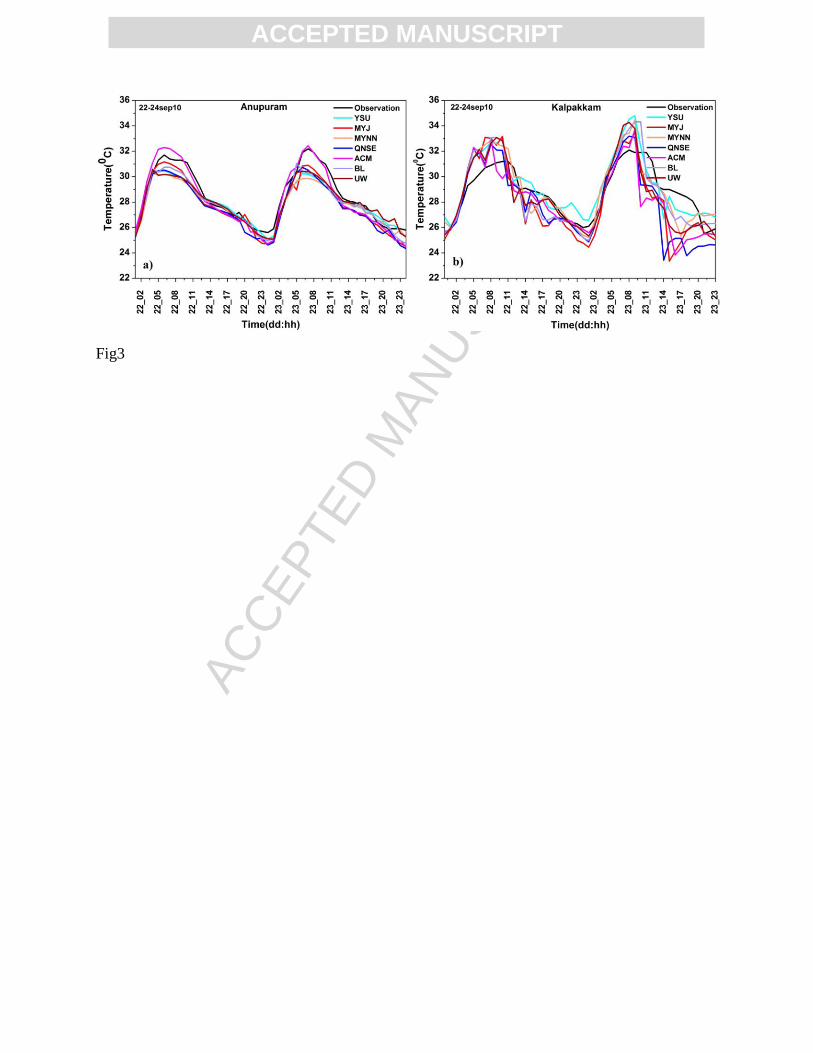
a) Diurnal evolution of Surface variables: The time variation of the surface level meteorological

variables simulated by ARW at Anupuram and Kalpakkam stations along with observations are

presented in Figures 3-6. The diurnal wavy pattern in surface level temperature, humidity and

winds could be simulated as in observations at both the stations. However, the magnitudes of

simulated variables differed among various schemes. Most PBL schemes produced a warm bias

in the daytime air temperature and a slight cold bias in the night time air temperature. Among the

ACC

EPTE

D M

ANU

SCR

IPT

ACCEPTED MANUSCRIPT

non-local schemes the ACM2 scheme simulated considerable overestimation of daytime

temperature and a small underestimation in the night time temperature. The YSU produced a

slight warm bias in both day and night temperatures. Among the higher order schemes MYNN

produced a slight warm bias and simulated the night time temperature in better agreement with

observations than other TKE schemes. The local closures MYJ, QNSE, UW, BL produced

considerable warm and cold biases in the day and night time temperatures. The MYJ and QNSE

simulated the largest clod and warm bias in the air temperatures. At the inland station Anupuram

most PBL schemes produced a slight cold bias and the ACM2 scheme produced a warm bias in

day temperature. Shin and Hong (2011) also reported warmer bias with ACM2 scheme and a

cold bias with QNSE while comparing with observations during the convective time. Surface

level relative humidity comparisons (Figure 4) shows that humidity was underestimated with all

the PBL schemes at both the stations. Underestimation of humidity by MYJ and YSU schemes

was also reported by Misenis and Zhang (2010) in air quality simulations over the coastal

Mississippi. YSU, MYNN, MYJ, QNSE and BL schemes exhibited lower dry bias in both day

and night time humidity relative to other schemes. The non-local scheme ACM2 produced a

large dry bias in both day and night time humidity. Among the TKE schemes MYJ and QNSE

simulated humidity in better agreement with the observations followed byBL, MYNN and UW.

Overall MYJ and QNSE simulated the surface relative humidity reasonably well. The above

results are similar to those found in Hu et al. (2010) in Texas (USA) and in Garcıa-Dıez et al

(2013) over Europe. The above studies also reported significantly less bias with YSU than MYJ,

ACM2 for temperature, humidity. The comparisons indicate that the differences among surface

thermodynamic variables from different schemes were maximum at daytime and minimum at

nighttime as also found in Shin and Hong (2011).

ACC

EPTE

D M

ANU

SCR

IPT

ACCEPTED MANUSCRIPT

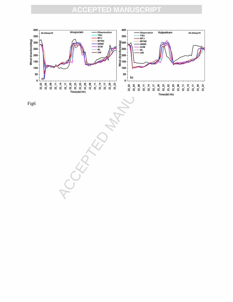
The time variation of winds at 10-m level from different experiments (Figure 5) indicated

considerable overestimation of winds with MYJ, QNSE in both day and nighttime. The other

schemes YSU, MYNN, BL, UW and ACM2 produced moderately stronger winds in both day

and night time relative to observed winds at both stations. Overestimation of winds with WRF

was also reported by Steeneveld et al (2008). Overall the ACM2 produced lesser deviations in

both day and night time wind speed simulations. Wind speed predictions with YSU, MYNN, BL

were better at Kalpakkam than at Anupuram. MYJ and QNSE simulated the highest wind speed

errors at both the stations. Unlike in Shin and Hong (2011) where the wind components were

more divergent at nighttime, present study shows the winds from different schemes were

divergent at the tropical site in both daytime and nighttime with large deviations from

observations. There were large directional shears in the simulations MYJ, QNSE in the initial

time period (Figure 6). Unlike at Anupuram the directional deviations of about 25-50 deg were

found with all the PBL schemes for the coastal site Kalpakkam, which could be due to the abrupt

contrast of land-water terrain at the Kalpakkam site. Barring these few deviations all the PBL

schemes well simulated the windflow direction.

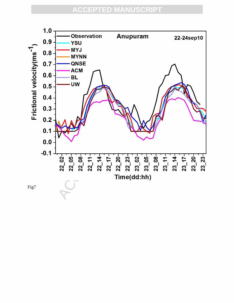
The differences in the simulated surface level winds and thermodynamical variables can

be explained from the differences in the friction velocity (u*) and surface fluxes. Comparison of

time variation of u* (Figure 7) indicated that the frictional velocity was generally underestimated

indicating underprediction of the shear force in the surface boundary layer in all simulations. The

u* values simulated by YSU, MYNN, BL were nearly similar which is due to the use of a

common surface layer scheme in the above simulations. The ACM2 and UW schemes that use

their respective surface layer schemes (Pleim-Xue, UW M-O theory) produced large

underestimation of frictional velocity. The variation in exchange coefficients and friction

ACC

EPTE

D M

ANU

SCR

IPT

ACCEPTED MANUSCRIPT

velocity can influence simulated sensible heat fluxes. The sensible heat and latent heat flux

comparisons show that a large bias is simulated in the daytime flux by various schemes (Figure

8). All the PBL schemes overestimated the sensible heat flux on the first day of simulation and

an improvement was noted in the simulated heat flux on the second day. This could be due to

certain spinup time taken by the Noah land surface model for adjusting to the soil and vegetation

processes to evolve the surface fluxes. While all the schemes similarly simulated the night time

fluxes the MYJ, QNSE, ACM2 schemes produced higher daytime fluxes relative to observed

fluxes. Further the latent heat flux was almost comparable in magnitude to sensible heat which

could be due to high soil moisture and transfer of energy by evaporative process in the coastal

environment. Overall, the MYNN and YSU show a better comparison of the surface heat flux

simulation. The same time variations were found in the latent heat flux simulation and the

schemes MYNN, YSU produced better latent heat flux simulations. The higher/lower sensible

heat flux in QNSE/YSU in convective condition may be attributed to the simulated surface

exchange coefficients in the respective schemes (Shin and Hong, 2011).

b) Boundary layer flow field: The simulated surface level (10 m) flow field from the fine nest is

analysed during the unstable daytime at 12 IST (Figure 9). In the morning conditions calm

westerly flow (~1 ms-1

) was simulated over the land in all the experiments and the winds were

slightly stronger (1 to 1.5 ms-1

) over the ocean relative to the land (0.5 to 1.5 ms-1

) region.

During the daytime large variations were found in the simulated surface temperature and flow

field in different simulations. Large air temperature gradients (~5-7°C) across the land and sea

interface at the coast were found in the simulations ACM2, MYJ, QNSE. Correspondingly

stronger sea breeze with ACM2, MYJ, QNSE (4-5 ms-1

) and weaker winds with YSU, MYNN,

BL, UW (2 to 3 ms-1

) were simulated. The relatively higher atmospheric temperatures simulated

ACC

EPTE

D M

ANU

SCR

IPT

ACCEPTED MANUSCRIPT

with ACM2, MYJ, QNSE indicated relatively higher convective turbulence, higher diffusion and

therefore a relatively deep boundary layer formation in these cases. Sea breeze flow was more

organized with YSU, ACM2, MYNN, UW and was highly divergent in the cases MYJ, QNSE,

and BL. The vertical extent of the sea breeze was found up to 700 m with MYJ, QNSE, and up to

400 m / 500 m in the other cases (not shown). Factors such as PBL height, wind shear, and

entrainment of free atmospheric air into the PBL affect the wind distribution and mesoscale

circulations (Arya, 2001). These factors are inturn related to the surface fluxes and PBL

diffusivities which are analysed further in the following discussions.

c) Vertical PBL structure: Vertical profiles of simulated potential temperature, relative

humidity, wind speed and wind direction at 06 IST, 12 IST, 16 IST corresponding to morning,

daytime and sea breeze time in the afternoon for Anupuram station are shown in Figures 10, 11 ,

12 and 13 respectively. The potential temperature profiles indicate slight overestimation in the

temperature during the morning time. Above 50 m, highly stable conditions were simulated with

all the PBL schemes giving similar vertical temperature variation in the morning as in

observations. The local-closures QNSE, MYJ, UW, and BL produced highly stable conditions

compared to other schemes. During the convective conditions at 12 IST the radiosonde data

indicate development of a well mixed layer growing up to 900 m above ground level (AGL). A

shallow unstable surface layer (extending to ~100 m AGL) was also found. The profiles with

MYJ, BL, UW indicated a shallow 600 m deep mixed layer , YSU, MYNN indicated 800 m deep

mixed layers whereas ACM2 and QNSE produced deeper (~1000 m) convective layers. During

the sea breeze hours the potential temperature profiles show shallow convective mixed layer with

a vertical extent of about 400 m AGL. This shallow mixed layer during sea breeze is well known

as the thermal internal boundary layer (TIBL) in coastal regions. The development of sea breeze

ACC

EPTE

D M

ANU

SCR

IPT

ACCEPTED MANUSCRIPT

in the afternoon at the coastal site can be recognized from a change in the wind direction from

southwesterly (~225) to southeasterly (~120), strengthening of the winds from 3 ms-1

to 5 ms-1

and increase in the relative humidity from 50% to 80%. While ACM2 produced a deeper (~750

m deep) mixed layer during the sea breeze time, the experiments QNSE, MYJ, UW produced

relatively shallow mixed layers (<400 m deep) than that was found in the actual profile. Of all

the seven experiments YSU, MYNN, BL well simulated the mixed layer (350 m deep)

characteristics during the sea breeze time. Well developed deep convective mixed layers using

YSU, and shallow layers with MYJ were also reported by Misenis and Zhang (2010) in air

quality simulations using WRF-Chem.

With reference to the relative humidity, the profile comparisons show vertically decreasing

humidity in the morning, increasing humidity in the convective daytime up to 1000 m AGL at 12

IST and up to 400 m AGL during the sea breeze hours. The morning humidity profiles ingeneral

show a steep unstable surface layer with humidity drastically falling up to 100- 150 m AGL and

then increasing to a height of 400 m AGL. The MYNN, YSU, UW and to some extent the

ACM2 experiments produced these stable layer humidity characteristics well, while the rest of

the simulations (MYJ, QNSE, BL) produced a continuously falling humidity in the lower

atmosphere. Observations at this time, however, were erroneous which may be due to the failure

of the humidity sensor of the Radiosonde. During the convective daytime conditions the

humidity profiles given by QNSE, ACM2 indicated an increasing moist bias with height as in the

case of temperature. The vertical variations of humidity simulated with MYJ, UW and BL were

indicative of a relatively shallow (~500 m deep at 12 IST; ~250 m deep at 16 IST) mixed layer

development in comparison to the observed layer with radiosonde. The humidity profiles

simulated with MYNN and YSU were more realistic both in convective noon time (12 IST) as

ACC

EPTE

D M

ANU

SCR

IPT

ACCEPTED MANUSCRIPT

well as during sea breeze time (16 IST). The simulated thermodynamic properties show that

QNSE, ACM2, YSU, UW generally produced dry and warm layers which could be due to

excessive mixing (by larger eddy exchange coefficient for heat and moisture) computed in these

schemes. The other schemes MYJ, MYNN, BL produced relatively cold and humid layers. The

above results of YSU simulating slightly more warm and dry layers than MYJ are consistent

with those obtained by Hu et al (2010) using WRF over Texas and Kim et al (2006) using WRF-

Chem in airquality study. The deficiencies in reproducing the temperature and humidity by

various schemes at the coastal site in the present study could be attributed to the deficiencies in

capturing small-scale meteorological phenomena under complex weather patterns involving

land/sea interactions as was also reported by Misneis and Zhang (2010).

Comparison of wind speed profiles (Figure 12) shows that during the stable morning

conditions all the simulations overestimated wind speed in the first 600 m AGL. Here, the

ACM2, MYNN and YSU indicate better comparisons than the other experiments. Above 600 m

most of the simulations produced lower wind speeds than the observations except ACM2 and

UW. Similarly, during the convective daytime conditions except ACM2 all the experiments

especially QNSE and MYJ produced higher wind speed in the lower 400 m region of the

atmosphere. In the layer above 400 m AGL the QNSE shows a better comparison than the other

schemes. During the sea breeze (16 IST) the same pattern of vertical variation of wind speeds as

at noon time were found in the simulations. Overall, the YSU, MYNN, BL, ACM2 schemes

produced better wind speed comparisons than the rest. The large differences between simulated

and observed wind profiles in the layer above 600 m could be due to the horizontal drift of the

radiosonde from its release location.

ACC

EPTE

D M

ANU

SCR

IPT

ACCEPTED MANUSCRIPT

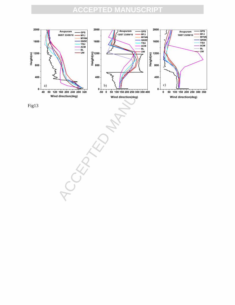
Comparison of the vertical variation of wind direction (Figure 13) indicated that all the

simulations well produced the vertical wind directional shear in the boundary layer. All the

schemes indicate westerly / southwesterly boundary layer flow in the late night/ morning time

and the occurrence of sea breeze in the 0-500 m layer in the daytime. The simulated direction

profiles with YSU, QNSE, BL and MYNN were in better agreement with observations than the

others in both stable and unstable conditions. The direction comparisons clearly show

southeasterly sea breeze flow simulation in the lower levels up to 500 m AGL in agreement with

observations. ACM2 produced slightly higher shear than other schemes at about 1 km region.

Santos-Alamillos et al (2013) in a study of wind flow with WRF over southern Spain showed the

wind direction estimates were more sensitive to the terrain characteristics rather than the model

physics. Our present results also show less direction deviations with different PBL physics for

the coastal site.

c) Time Evolution of PBL: Intercomparison of the time-height variations from 00 UTC 22 to 00

UTC 24 September 2010 in potential temperature (θ) (Figure. 14) and specific humidity (q)

(Figure 15) for the model grid at Kalpakkam indicates the model simulated the evolution of the

boundary layer generally well in all the PBL schemes, but with some differences. During the

period from local night (00 IST / 18 UTC) to local morning (08 IST/ 02 UTC) the simulated

mean potential temperature increased with height indicating stable statification in all the cases.

Both the local as well as the non-local diffusion schemes similarly produced the nocturnal

boundary characteristics at the observation site. At around 06 IST/ 00 UTC all the simulations

showed highly stable temperataure stratification and the local closures (MYJ, QNSE, BL, UW)

more clearly depicted the stable boundary layer formation in agreement with the corresponding

Radiosonde observations (Figure 10a). In the daytime from 09 IST/03 UTC onwards the

ACC

EPTE

D M

ANU

SCR

IPT

ACCEPTED MANUSCRIPT

potential temperature remained uniform up to a certain height and then increased from 0.6 km

upwards indicating development of well mixed conditions from 09 IST onwards. The layer

within which the temperataure remained uniform had reduced from 0.6 km to 0.4 km at 12 IST/

06 UTC and further to 0.2 km at 15 IST/ 09 UTC. This alteration in the mixed layer depth to a

minimum value in the afternoon is a unique feature of coastal locations and is due to the well

known phenomena of TIBL formation at the coast. The vertical extent of the daytime convective

(or unstable) boundary layer was variously simulated in different experiments. The well mixed

layer height was simulated as 0.6 km with YSU, MYJ, MYNN; 0.7 km with ACM2, 0.9 km

with QNSE, 0.55 with UW, BL schemes. The QNSE, produced the deepest boundary layer

followed by ACM2, YSU, MYNN, MYJ, BL, UW schemes. The PBL schemes QNSE, ACM2

and UW produced extremities (deep/shallow) in mixed layer simulations. The above results of

formation of deeper convective boundary layers with QNSE, ACM2; shallow layers with UW

and moderately deep conective layers with YSU, MYNN, BL, MYJ schemes were supported by

Radiosonde observations in the earlier discussion. Simulation of deep boundary layers with

ACM2 and moderately deep layers with YSU and MYJ were also reported by Garcıa-Dıez et al

(2013) over Europe.

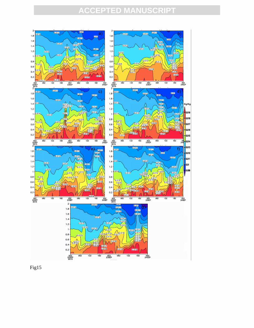
The diurnal evolution of the PBL could also be analysed from the time-height variations in

specific humidity (Figure 15). The stable boundary layers during the night and morning were

marked with decreasing specific humidity whereas the unstable layers in the daytime were

marked with near uniform vertical humidity distribution. The deepest boundary layers during the

daytime were found with QNSE followed by ACM2, MYJ, YSU, MYNN, BL and UW. The

local closure TKE schemes (MYJ, MYNN, QNSE, BL and UW) produced steep vertical

gradients in the humidity distribution during the night stable atmospheric conditions (at 03 IST/

ACC

EPTE

D M

ANU

SCR

IPT

ACCEPTED MANUSCRIPT

21 UTC) as compared to the non-local schemes. However, the non-local schemes produced

distinctly uniform humidity distributions during the convective day time conditions (12 IST/06

UTC) as compared to the local-closure schemes thus showing the expected well mixed

conditions. The local schemes produced relatively higher humidity (0.019 kg/kg) in the lower

layers as compared to the non-local schemes (~0.017 kg/kg) under convective conditions

indicating lesser mixing as compared to the non-local schemes.

d) PBL Height: Various methods are used in model PBL formulations for the estimation of

boundary layer height involving thermodynamics, dynamics, using parameters like the critical

Richardson number, threshold TKE, potential temperature etc (e.g., Noh et al. 2003; Troen and

Mahrt, 1986; Vogelezang and Holtslag, 1996; Shin and Hong, 2011). The PBL height is

diagnosed from bulk Richardson number by comparing with critical Richardson number in YSU

and ACM2 schemes. In YSU scheme bulk Richardson number is calculated from the surface. For

convective conditions its value is set to zero, whereas in stable conditions Ri is taken > 0 (0 to

0.25). In the case of ACM2, PBL is considered to comprise a free convective layer and an

entrainment layer. The height of free convective layer is diagnosed from the temperature of the

rising plume. The height at which the temperature of the rising plume is equal to the temperature

of the surrounding environment is considered as the top of the free convective layer. The depth

of the entrainment layer estimated from the critical Richardson number is added to the height of

the free convection layer to obtain the height of the PBL. In the case of local PBL schemes (i.e.,

MYJ, QNSE, MYNN, BL, UW), PBL height is diagnosed as the height where prognostic TKE

reaches a sufficiently small value (of the order of 0.005 m2/s

2) (Shin and Hong, 2011). In the

present study the PBL height was analysed from daytime Radiosonde observations using

potential temperature profile specifically for the morning (06 IST) and noon (12 IST) conditions.

ACC

EPTE

D M

ANU

SCR

IPT

ACCEPTED MANUSCRIPT

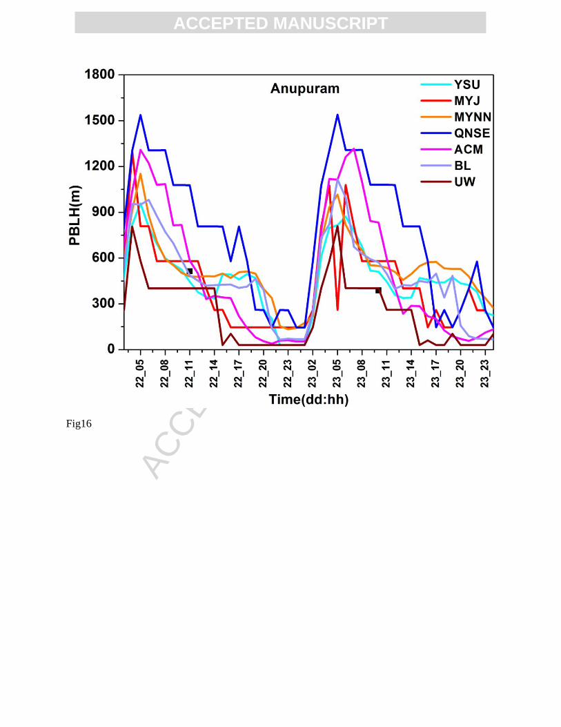
The comparison shows that during daytime the QNSE, ACM2 simulated very deep boundary

layers, UW simulated shallow PBL while MYJ, MYNN, YSU, BL simulated intermediately

deep layers (Figure. 16). During the night time while ACM2, BL, YSU, UW produced very

shallow layers MYNN, QNSE, MYJ simulated unrealistic deep layers. The time variations show

that while ACM2, QNSE, MYJ, UW produced a sudden decay of PBL around the day/night

transition (15IST), the MYNN,YSU, BL schemes simulated extended mixed layers through night

indicating a gradual decay of PBL and higher nocturnal PBL height (439 m to 575 m) (Table 2).

During the stable morning conditions the local closures (QNSE,MYJ, MYNN, BL) except UW

produced deeper layers in contrast to the non-local schemes YSU and ACM2 (Table 2).

However, during the daytime, except QNSE and MYJ, the local closures produced relatively

shallow convective layers in comparison to the non-local closures. Among nonlocal PBL

schemes ACM2 produced deeper boundary layers (PBL height: 1262.8m/59m) relative to the

YSU (PBL height: 871.9m/29.97m) during both e convective and stable conditions. Among the

local PBL schemes QNSE produced very deep boundary layers (PBL height: 1308m/259m) and

UW produced shallow (PBL height: 402m/29m) boundary layers during the convective and

stable conditions respectively indicating extremities. From the diurnal cycle the YSU, MYNN,

BL schemes produced more realistic time variation in the PBL heights in better agreement with

profile observations. Shin and Hong (2011) while evaluating WRF PBL formulations with

CASES observations also reported simulation of deep mixed layers with QNSE, ACM2, MYJ;

moderate layers with YSU and shallow layers with BL. Our present results from the tropical site

corroborate findings of the above study.

e) Eddy diffusivities: The differences in the simulation of dynamic and thermodynamic variables

in the lower atmosphere could be related to the variation in the simulation of the eddy exchange

ACC

EPTE

D M

ANU

SCR

IPT

ACCEPTED MANUSCRIPT

coefficients for momentum (Km) and heat / moisture (Kh) by various schemes. We analysed the

Kh, Km parameters from various schemes and presented in Figure 17 and Table 3. Among the

seven PBL schemes used ACM2 and BL assume the eddy diffusivity for momentum as identical

to that for enthalpy (Prandtl number Km/Kh ~1) whereas in MYJ, MYNN, QNSE, YSU and UW

schemes Kh is larger than Km. Under unstable conditions or strong shear the assumption of

Km=Kh may not be valid. The time averaged Km, Kh for the period (01 UTC-19 UTC)

representing unstable conditions and for the period (19 UTC 22 September 2010 - 01UTC 23

September 2010) representing stable conditions are presented in the above figure. Each TKE

scheme used a different approach to calculate S and l parameters used in the expression for K. As

expected though all the schemes indicated higher eddy diffusivities during unstable regime

relative to the stable regime the ACM2, MYNN and UW produced higher Km and Kh values

relative to other PBL schemes. While the ACM2, UW produced the largest diffusivities, the BL

and QNSE simulated least diffusivities indicating extremities in turbulent mixing in the above

schemes. The Km values with ACM2, UW were about 5 times higher relative to most PBL

schemes. This had lead to stronger simulated winds with QNSE, MYJ schemes relative to the

ACM2, UW as discussed earlier. Similarly the Kh was comparatively higher in ACM2, UW

which tend to produce higher mixing of heat or moisture and hence warmer and dry boundary

layer. During the stable atmospheric conditions the simulated Km, Kh were nearly of the same

order of magnitude and ACM2, UW produced slight higher values of Km, Kh. Hence in stable

atmospheric conditions the simulated quantities from all the schemes nearly converged. Thus in

general ACM2, UW simulated higher diffusivities for momentum and heat/ moisture in

comparison to MYJ, YSU, MYNN, QNSE, BL which resulted in variations in the simulated PBL

parameters. Overall the Km, Kh values simulated with YSU, MYNN schemes are in the

ACC

EPTE

D M

ANU

SCR

IPT

ACCEPTED MANUSCRIPT

intermediate range of the seven PBL schemes in both stable and convective conditions and hence

produced lesser errors in the simulated mean variables.

The mean model error statistics from various PBL simulations for different variables are

presented in Table 4. As discussed earlier YSU/MYNN has shown better results in 2m-

temperature prediction (RMSE=1.03/1.123, Bias=-0.004/-0.28) and MYJ/QNSE has shown

largest cold bias (-0.68/-0.84; RMSE =1.33/1.43) relative to other schemes. For humidity,

MYJ/QNSE showed less dry bias (-9.59/-9.76) and less RMSE (11.88/12.08) relative to other

schemes. In the case of 10m-wind speed, ACM2 produced least bias 0.35 and RMSE (1.19) and

MYJ/QNSE generated largest biases (1.44/1.37) and RMSE (1.87/1.79) of various PBL schemes.

6. Conclusions

In this study numerical simulations were conducted with WRF-ARW mesoscale model to

study the Planetary Boundary Layer characteristics at the tropical site Kalpakkam on the

southeast coast of India. The ability of the model to reproduce the observed features was studied

by conducting simulations with seven PBL schemes and by intercomparison. The observations

collected during an intensive field measurement campaign RRE were used to verify the results

from different numerical experiments. Diagnosis of the surface level meteorological variables

(winds, temperature, humidity, surface fluxes) and their vertical variation indicated that for

temperature the non-local PBL scheme YSU and the higher order local-closure TKE scheme

MYNN produced better results. For humidity MYJ, MYNN, QNSE simulated reasonably well

while ACM2, YSU produced large dry bias in the night time. For wind speed the combined

local/ non-local scheme ACM2 produced better simulations, and local closures MYJ, QNSE

considerably overestimated the winds while the other schemes (YSU, MYNN, BL, UW)

ACC

EPTE

D M

ANU

SCR

IPT

ACCEPTED MANUSCRIPT

simulated moderately stronger winds relative to observations. However, all the PBL schemes

reproduced the wind direction reasonably well. Though large underestimation of friction

velocity was found in the case of ACM2 , the higher eddy diffusivities found with ACM2 seem

to provide better wind simulations than the other cases.

While all the PBL schemes well simulated the stable morning profiles, there were large

differences in the convective daytime profiles. The vertical extents of unstable surface layer, well

mixed layer and inversion layer were differently simulated by different PBL parameterizations.

A wide variation was found in the simulated PBL heights by different schemes. Relatively

shallow convective boundary layers with UW (402 m), very deep mixed layers with ACM2,

QNSE (1200m to 1308m) and moderately deep layers with YSU,BL,MYJ, MYNN (800m to

1070m) were simulated. This variation in mixing height simulation could be due to the use of

different formulations for PBL height in different schemes. Considering the diurnal cycle the

YSU, BL, MYNN schemes produced more realistic time variation in the PBL heights in better

agreement with radiosonde profile data. Of all the seven experiments YSU and MYNN well

simulated the mixed layer characteristics (lesser temperature, higher humidity, moderate winds)

during the sea breeze time. A wide variation of diffusivities (Kh, Km) was produced

by different PBL schemes which had led to variations in the vertical extent

of mixed layer, magnitudes of thermodynnamical variables and momentum.

The ACM2, UW, MYNN simulated higher diffusivities than MYJ, YSU, QNSE, BL for

momentum and heat/ moisture in both stable and unstable atmospheric conditions. The higher

exchange coefficients in the case of ACM2, UW, MYNN produced relatively lesser winds, warm

and dry mixed layers in these cases in comparison to the other PBL schemes. The Km, Kh values

from YSU, MYJ and BL were in the intermediate range of the seven PBL schemes and they

ACC

EPTE

D M

ANU

SCR

IPT

ACCEPTED MANUSCRIPT

produced lesser errors in the simulated mean variables. The variations in the simulated quantities

could be partly also due to the variation in the use of different surface layer formulations with

different PBLs as evident from the variation in the simulated friction velocity and surface fluxes.

A comprehensive examination of all the schemes in the present study indicated that no

scheme perfectly works for all the variables and for all the stability conditions. In general the

observational comparison indicated the non-local scheme YSU produced more realistic

atmospheric structures during the convective conditions and the TKE closures MYNN produced

more realistic vertical structures during the stable conditions. These results corroborate the

findings from earlier intercomparison studies by Hu et al. (2010), Shin et al. 2011 and

Steeneveld, (2008) with WRF model. The simulations in the present study were focused on a

warm convective period at the tropical coastal site. The boundary layer structure simulated by

WRF needs to be assessed for a stable cold season as well as an inland station to further study

the performance of the PBL schemes in tropical conditions. It is also required to use continuous

observations like Wind profiler to assess the temporal evolution of the PBL simulated by the

model.

Acknowledgements:

Authors thank S.A.V. Satya Murty, Director, EIRSG, for the encouragement in carrying out the

study. The observations used in the study were obtained from the Round Robin Exercise project

coordinated by IGCAR and funded by Board of Research in Nuclear Sciences, DAE, Mumbai.

Authors acknowledge NCEP/NOAA for the public access of GFS analysis/forecasts used in the

study. ARW model was obtained from NCAR, USA. Thanks are due to anonymous reviewers

for their technical comments which helped to improve the manuscript.

References:

ACC

EPTE

D M

ANU

SCR

IPT

ACCEPTED MANUSCRIPT

Arya, S.P. 2001. Introduction to Micrometeorology. Academic Press, Apr 25, 2001, 420 pp.

Berg, L.K., Zhong, S., 2005. Sensitivity of MM5-simulated boundary layer characteristics to

turbulence parameterizations. J. Appl. Meteorol. 44 (9),1467–1483.

Bhaskar Rao, D.V., Hari Prasad, D., 2006. Numerical prediction of the Orissa super-cyclone

(1999): Sensitivity to the parameterization of convection, boundary layer and explicit moisture

processes. Mausam. 57(1), 61–78.

Blackadar, A.K., 1979. High-resolution models of the planetary boundary layer. in : Pfafflin,

J.R., Ziegler, E.N. (Eds.), Adv. Environ. Sci. Eng. vol.1, Gordon and Breach Science Publishers,

pp. 50-85.

Bougeault, P., Lacarrére, P., 1989. Parameterization of orography-induced turbulence in a

mesobeta-scale model. Mon. Weather Rev. 117, 1872–1890.

Bright, D. R., Mullen, S.L., 2002. The sensitivity of the numerical simulation of the southwest

monsoon boundary layer to the choice of PBL turbulence scheme in MM5. Wea. Forecasting, 17,

99–114.

Braun, S. A., Tao, W.K., 2000. Sensitivity of high-resolution simulations of Hurricane Bob

(1991) to planetary boundary layer parameterizations. Mon. Weather Rev. 128, 3941–3961.

Bretherton, C.S., Park, S., 2009. A new moist turbulence parameterization in the Community

Atmosphere Model. J. Climate. 22, 3422-3448.

Burk, S.D., Thompson, W.T., 1989. A vertically nested regional numerical prediction model

with second-order closure physics. Mon. Weather Rev. 117, 2305–2324.

Chen, F., Pielke R. Sr., Mitchell, K., 2001. Development and application of land-surface models

for mesoscale atmospheric models: in: Lakshmi, V., Alberston, J., Schaaake., (Eds.), Problems

and Promises. Observation and Modeling of the Land Surface Hydrological Processes, American

Geophysical Union, 107-135.

Fast, J.D., O’Steen, B.L., Addis, R.P., 1 5. Advanced atmospheric modeling for emergency

response. J. Appl. Meteorol. 34 (3), 626-649.

Garratt, J.R., 1994. The Atmospheric Boundary Layer. Cambridge Atmospheric and Space

Science Series. 316 pp.

Garcıa-Dıez M, Fernandez J, Fita L. Yague C. 13. Seasonal dependence of WRF model biases

and sensitivity to PBL schemes over Europe. Q. J. R. Meteorol. Soc. 139: 501–514.

DOI:10.1002/qj.1976

ACC

EPTE

D M

ANU

SCR

IPT

ACCEPTED MANUSCRIPT

Galperin B, Sukoriansky S (2010) Progress in turbulence parameterization for geophysical flows.

In: The 3rd

international workshop on Next-generation NWP models: bridging parameterization,

explicit clouds, and large eddies. Seoul, Korea,

5.4.http://nml.yonsei.ac.kr/20100829/content/agenda.html.

Gopalakrishnan, S.G., Frank, M., Zhang, J.A., Zhang, X., Bao, J.W., Tallapragada, V., 2013. A

Study of the Impacts of Vertical Diffusion on the Structure and Intensity of the Tropical

Cyclones Using the High-Resolution HWRF System. J. Atmos. Sci. 70, 524–541. doi:

http://dx.doi.org/10.1175/JAS-D-11-0340.1

Holtslag, A.A., Boville, B.A., 1993. Local versus nonlocal boundary layer diffusion in a global

climate model. J. Climate. 6, 1825-1842.

Hong, S.Y., Pan, H.L., 1996. Nonlocal boundary layer vertical diffusion in a Medium-Range

Forecast model. Mon. Weather Rev. 124, 2322-2339.

Hong, S.Y., Noh, Y., Dudhia, J., 2006. A new vertical diffusion package with an explicit

treatment of entrainment processes. Mon. Weather Rev. 134, 2318–2341

Hu, X.M., Nielson-Gammon, J.W., Zhang, X., 2010. Evaluation of Three Planetary Boundary

Layer Schemes in the WRF Model. J. Appl. Meteorol. 49, 1831-1844.

Janjic, Z.A., 1990. The step-mountain coordinate: physics package. Mon Weather Rev

118:1429–1443.

Janjic, Z.A., 1994. The step-mountain ETA coordinate model: further development of the

convection, viscous sublayer and turbulence closure scheme. Mon. Weather. Rev. 122(5), 927–

945.

Jimenez, P., Jorba, O., Parra, R., Baldasano, J.M., 2006. Evaluation of MM5‐EMICAT2000‐CM

AQ performance and sensitivity in complex terrain: High‐resolution application to the nort

heastern Iberian Peninsula. Atmos. Environ. 40, 5056‐5072.

Kain, J.S., Fritsch, J.M., 1993. Convective parameterization for mesoscale models: the Kain-

Fritcsh scheme, in: Emanuel, K.A., Raymond, D.J. (Eds.), The Representation of Cumulus

Convection in Numerical Models. American Meteorological Society, Boston, MA, USA.

Kim, S-W., McKeen, S.A., Hsie, E.Y., Trainer, M.K., Frost, G.J., Grell, G.A., Peckham, S.E.,

2006. The Influence of PBL parameterizations on the distributions of chemical species in a

mesoscale chemical transport model, WRF-Chem. 17th Symposium on Boundary Layers and

Turbulence. American Meteorological Society, 21 May 2006. Abstract. J3.3

(https://ams.confex.com/ams/pdfpapers/111150.pdf)

ACC

EPTE

D M

ANU

SCR

IPT

ACCEPTED MANUSCRIPT

Madala, S., Satyanarayana, A.N.V., Narayana Rao, T. 2014. Performance evaluation of PBL and

cumulus parameterization schemes of WRF-ARW model in simulating severe thunderstorm

events over Gadanki MST radar facility — Case study. Atmos. Res.139, 1-17.

Mellor, G.L., Yamada, T., 1982. Development of a turbulence closure model for geophysical

fluid problems. Rev. Geophys. Space Phys. 20, 851–875.

Misenis, C., Zhang, Y. 2010. An examination of sensitivity of WRF/Chem predictions to

physical parameterizations, horizontal grid spacing, and nesting options. Atmos. Res. 97, 315–

334.

Mlawer, E.J., Taubman, S.J., Brown, P.D., Iacono, M.J., Clough, S.A., 1997. Radiative transfer

for inhomogeneous atmosphere: RRTM, a validated correlated-k model for the longwave. J.

Geophys. Res. 102, 16663-16682.

Montgomery, M. T., Smith, R. K., Nguyen, S., 2010. Sensitivity of tropical cyclone models to

the surface drag coefficient. Q. J. Roy. Meteorol. Soc. 136, 1945-1953.

Mukhopadhyay, P., Taraphdar, S., Goswami, B.N., Krishnakumar, K., 2010. Indian summer

monsoon precipitation climatology in a high-resolution regional climate model: Impacts of

convective parameterization on systematic biases. Weather Forecast. 25(2), 369-387.

Nakanishi, M., Niino, H., 2004. An improved Mellor-Yamada level-3 model with condensation

physics: Its design and verification. Bound. Layer Meteorol. 112, 1–31.

Noh, Y., Cheon, W. G., Hong, S. Y., Raasch, S., 2003. Improvement of the K-profile model for

the planetary boundary layer based on large eddy simulation data. Bound. Layer Meteorol. 107,

401–427.

Nolan, D.S., Zhang, J.A., Stern, D.P., 2009a. Evaluation of planetary boundary layer

parameterizations in tropical cyclones by comparison of in-situ data and high-resolution

simulations of Hurricane Isabel (2003). Part I: Initialization, maximum winds, and outer core

boundary layer structure. Mon. Weather. Rev. 137, 3651–3674.

Nolan, D.S., Zhang, J.A., Stern, D.P., 2009b. Evaluation of planetary boundary layer

parameterizations in tropical cyclones by comparison of in-situ data and high-resolution

simulations of Hurricane Isabel (2003). Part II: Inner core boundary layer and eyewall structure.

Mon. Weather. Rev. 137, 3675–3698.

Pleim J.E., 2006. A simple, efficient solution of flux–profile relationships in the atmospheric

surface layer. J Appl Meteorol Clim 45:341–347

Pleim, J.E., 2007. A combined local and non-local closure model for the atmospheric boundary

layer. Part 1: Model description and testing. J. Appl. Meteorol. Climatol. 46, 1383–1395.

ACC

EPTE

D M

ANU

SCR

IPT

ACCEPTED MANUSCRIPT

Poulos, G.S., Blumen, W., Fritts, D.C., Lundquist, J.K., Sun, J., Burns, S.P., Nappo, C., Banta,

R., Newson, R., Cuxart, J., Terradellas, E., Balsley, B., Jensen, M., 2002. CASES-99: A

comprehensive investigation of the stable nocturnal boundary layer. Bull. Am. Meteorol. Soc.

83(4), 555–581.

Santos-Alamillos, F.J., Pozo-Va Zquez, D., Ruiz-Arias, J.A., Lara-Fanego, V., Tovar-Pescador.

J. 2013. Analysis of WRF Model Wind Estimate Sensitivity to Physics Parameterization Choice

and Terrain Representation in Andalusia (Southern Spain). J Appl Meteorology and

Climatology. Vol 52, 1592-1609.

Sanjay, J., 2008. Assessment of Atmospheric Boundary-Layer Processes represented in the

numerical model MM5 for a Clear Sky Day using LASPEX Observations. Bound. Layer

Meteorol, 129, 159-177.

Shin, H.H., Hong, S.Y., 2011. Intercomparison of Planetary Boundary-Layer Parameterizations

in the WRF Model for a Single Day from CASES-99. Bound. Layer Meteorol. 139, 261–281.

Skamarock W.C., Klemp, J.B., Dudhia J., Gill D.O., Barker D.M., Duda, M.G., Huang X.Y.,

Wang, W., Powers J.G., 2008. A description of the advanced research WRF Version 3. NCAR

Technical Note, NCAR/TN-475+STR. Mesoscale and Microscale Meteorology Division,

National Center for Atmospheric Research, Boulder, CO, USA.

Smith, R.K., Thomsen, G.L., 2010. Dependence of tropical-cyclone intensification on the

boundary-layer representation in a numerical model. Q. J. R. Meteorol. Soc. 136, 1671-1685.

Srinivas, C.V., Venkatesan, R., Bhaskar Rao, D.V., Hari Prasad, D., 2007a. Numerical

Simulation of Andhra Severe Cyclone (2003): Model Sensitivity to the Boundary Layer and

Convection Parameterization. Pure Appl. Geophys. 164, 1465-1487.

Srinivas, C.V., Venkatesan, R., Bagavath Singh, A., 2007b. Sensitivity of mesoscale simulations

of land-sea breeze to boundary layer parameterization. Atmos. Environ. 41, 2534-2548.

Srinivas, C.V., Bagavath Singh, A., Venkatesan, R., Baskaran, R., 2011. Creation of Benchmark

Meteorological Observations for RRE on Atmospheric Flowfield Simulation at Kalpakkam. IGC

Report – 213. Indira Gandhi Centre for Atomic Research, Kalpakkam 603102, Tamilnadu, India.

Srinivas, C.V., Bhaskar Rao, D.V., Yesubabu, V., Baskaran, R., Venkatraman, B., 2012a.

Tropical cyclone predictions over the Bay of Bengal using the high-resolution Advanced

Research Weather Research and Forecasting (ARW) model. Q. J. R. Meteorol. Soc.

DOI:10.1002/qj.2064.

ACC

EPTE

D M

ANU

SCR

IPT

ACCEPTED MANUSCRIPT

Steeneveld, G.J., Mauritsen, T., DeBruijn, E.I.F., De Arellano, J.V.G., Svensson, G., Holtslag,

A.A.M., 2008. Evaluation of limited-area models for the representation of the diurnal cycle and

contrasting nights in CASES-99. J Appl. Meteorol. Climatol. 47, 869–887.

Stensrud, D., 2007. Parameterization Schemes: Keys to Understanding Numerical Weather

Prediction Models. Cambridge University Press. 459 pp.

Stull, RB., 1988. An introduction to boundary layer meteorology. Kluwer, Dordrecht, Holland,

pp680.

Sukoriansky, S., Galperin, B., Perov, V., 2005. Application of a new spectral theory of stable

stratified turbulence to the atmospheric boundary layer over sea ice. Bound. Layer Meteorol.

117, 231–257.

Troen, I., Mahrt, L., 1986. A simple model of the atmospheric boundary layer: Sensitivity to

surface evaporation. Bound. Layer Meteorol. 37, 129-148.

Vogelezang, D. H. P., Holtslag, A. A. M., 1996. Evaluation and model impacts of alternative

boundary-layer height formulations. Bound. Layer Meteorol. 81, 245-269.

Yerramilli, A., Challa, V.S., Dodla, V.B.R., Dasari, H.P., Young, J.H., Patrick, C., Baham, J.M.,

Hughes, R., Hardy, M.G., Swanier, S.J., 2010.

Simulation of Surface ozone pollution in the Central Gulf Coast Region using WRF/Chem

model: sensitivity to PBL and land surface physics. Adv. Meteorol. Article ID 319138, pp.

24. doi:10.1155/2010/319138.

Yerramilli, A., Challa, V.S., Dodla, V.B.R., Myles, L., Pendergrass, W.R., Vogel, C.A., Tuluri,

F., Baham, J.M., Hughes, R., Patrick, C., Young, J., Swanier, S., 2012.

Simulation of surface ozone pollution in the Central Gulf Coastal region during summer synopti

c condition using WRF/Chem air quality model. Atmos. Pollut. Res. 3, 55‐71.

doi: 10.5094/APR.2012.005.

Zhang, D., Anthes, R.A., 1982. A high-resolution model of the planetary boundary layer—

sensitivity tests and comparison with SESAME-79 data. J Appl Meteorol 21:1594–1609

Zhang, Y., Liu, P., Pun, B., Seigneur, C., 2006. A comprehensive performance evaluation of M

M5‐CMAQ for the summer 1999 southern oxidants study episode ‐ Part I: Evaluation prot

ocols, databases, and meteorological predictions. Atmos. Environ. 40, 4825‐4838.

ACC

EPTE

D M

ANU

SCR

IPT

ACCEPTED MANUSCRIPT

LIST OF TABLES

S.No Table Title

1. Details of the model configuration

2. Comparison of simulated PBL height from different experiments

3. Comparison of diffusivity coefficients under different stability conditions from

experiments with different PBL schemes

4. Model error statistics

ACC

EPTE

D M

ANU

SCR

IPT

ACCEPTED MANUSCRIPT

LIST OF FIGURES

S.No Table Title

1. Domain specification used in ARW (a) and study area in the fine nest domain (b)

details of observation instruments.

2. Synoptic Weather conditions during the observation period (a) mean sea level

pressure and Winds at 925hPa (b) geopotential height (m) and Winds at 200hPa.

3. Time variation of the 2m level temperature at a) Anupuram and b) Kalpakkam

stations.

4. Time variation of the 2m level relative humidity at a) Anupuram and b) Kalpakkam

stations.

5. Time variation of the 10m level wind speed (ms-1

) at Anupuram and Kalpakkam

stations.

6. Comparison of Wind direction at 10 m level from different simulations along with

observations at a) Anupuram and b) Kalpakkam.

7. Time variation of friction velocity simulated at Anupuram station in different

numerical experiments.

8. Time variation of surface fluxes simulated in different numerical experiments a)

sensible heat flux (Watts/m2) and b) latent heat flux (Watts/m

2).

9. Simulated surface level flow-field at 12 IST (06UTC) 22 September 2010 from

simulations with different PBL schemes a) YSU b) ACM2 c) MYJ d) MYNN e)

QNSE f) BL and g) UW

10. Simulated vertical profiles of potential temperature at a) 06 IST, b) 12 IST and c) 16

IST 23 September 2010 at Anupuram along with GPS sonde profiles

11. Simulated vertical profiles of relative humidity at a) 06 IST, b) 12 IST and c) 16 IST

on 23 September 2010 at Anupuram along with GPS sonde profiles

12. Simulated vertical profiles of wind speed at a) 06 IST, b) 12 IST and c) 16 IST on 23

September 2010 at Anupuram along with GPS sonde profiles

13. Simulated vertical profiles of wind direction at a) 06 IST, b) 12 IST and c) 16 IST on

23 September 2010 at Anupuram along with GPS sonde profiles

14. Time-height section of potential temperature (θ) in 22-24 September 2010 at

Kalpakkam from different numerical experiments a)YSU, b)ACM2, c)MYJ,

d)MYNN, e) QNSE, f) BL g)UW. The temperature contours are drawn as (θ-273)

and shown in units of degrees Kelvin. Times indicated on the x-axis are in UTC.

15. Time-height section of specific humidity (kg/kg) in 22-24 September 2010 at

Kalpakkam from different numerical experiments a)YSU, b)ACM2, c)MYJ,

d)MYNN, e)QNSE, f)BL, g)UW. Times indicated on the x-axis are in UTC.

16. Time variation of PBL height in 22-24 September 2010 from simulations with

different PBL schemes along with observed PBL height (in dots) at Anupuram.

17. Eddy diffusivity coefficients Km (for momentum) and Kh(for enthalpy). The top

panels (a for Km; b for Kh) are for the unstable conditions and the bottom panels (c

for Km; d for Kh) are for the stable conditions.

ACC

EPTE

D M

ANU

SCR

IPT

ACCEPTED MANUSCRIPT

Fig1

ACC

EPTE

D M

ANU

SCR

IPT

ACCEPTED MANUSCRIPT

Fig2

ACC

EPTE

D M

ANU

SCR

IPT

ACCEPTED MANUSCRIPT

Fig3

ACC

EPTE

D M

ANU

SCR

IPT

ACCEPTED MANUSCRIPT

Fig4

ACC

EPTE

D M

ANU

SCR

IPT

ACCEPTED MANUSCRIPT

Fig5

ACC

EPTE

D M

ANU

SCR

IPT

ACCEPTED MANUSCRIPT

Fig6

ACC

EPTE

D M

ANU

SCR

IPT

ACCEPTED MANUSCRIPT

Fig7

ACC

EPTE

D M

ANU

SCR

IPT

ACCEPTED MANUSCRIPT

Fig8

ACC

EPTE

D M

ANU

SCR

IPT

ACCEPTED MANUSCRIPT

Fig9

ACC

EPTE

D M

ANU

SCR

IPT

ACCEPTED MANUSCRIPT

Fig10

ACC

EPTE

D M

ANU

SCR

IPT

ACCEPTED MANUSCRIPT

Fig11

ACC

EPTE

D M

ANU

SCR

IPT

ACCEPTED MANUSCRIPT

Fig12

ACC

EPTE

D M

ANU

SCR

IPT

ACCEPTED MANUSCRIPT

Fig13

ACC

EPTE

D M

ANU

SCR

IPT

ACCEPTED MANUSCRIPT

Fig14

ACC

EPTE

D M

ANU

SCR

IPT

ACCEPTED MANUSCRIPT

Fig15

ACC

EPTE

D M

ANU

SCR

IPT

ACCEPTED MANUSCRIPT

Fig16

ACC

EPTE

D M

ANU

SCR

IPT

ACCEPTED MANUSCRIPT

Fig17

ACC

EPTE

D M

ANU

SCR

IPT

ACCEPTED MANUSCRIPT

TABLES

Table .1. Details of the model configuration

Model WRF V3.4

Dynamics Primitive equation, non-hydrostatic, fully compressible, terrain following

Vertical resolution 50 sigma levels

Horizontal

resolution

27 km 9 km 3 km 1 km

Domains of interest 4.56-20.39 ºN

70.07-86.33 ºE

9.48-15.41 ºN

76.98-83.06 ºE

10.83-14.18 ºN

78.45-81.88 ºE

11.55-13.46 ºN

79.69-81.139 ºE

Radiation Dudhia scheme for short wave radiation

Rapid Radiative Transfer Model for long wave radiation

Surface-layer Monin-Obukhov similarity scheme (MM5 scheme, Eta scheme, Pleim-

ue MO similarity

Land Surface

scheme

NOAH Land Surface scheme

PBL turbulence YonSei University(YSU),Mellor-Yamada-Janjic(MYJ),Mellor-Yamada

Nakanishi-Niino(MYNN2.5), BouLac, UW (Bretherton and

Park),ACM2(Pleim),and Quasi-Normal Scale Elimination

Cloud microphysics WRF single moment 6-class scheme (WSM6)‏

Table 2. Comparison of simulated PBL height from different experiments

Expt No. PBL Height (m)

Morning Daytime Nocturnal

YSU 29.97 871.90 439.52

ACM2 59.05 1262.81 200.59

MYJ 145.84 1078.75 259.64

MYNN 154.68 818.53 575.10

QNSE 259.16 1308.06 146.68

BL 65.22 996.92 498.46

UW 29.94 402.93 30.13

ACC

EPTE

D M

ANU

SCR

IPT

ACCEPTED MANUSCRIPT

Table 3. Comparison of diffusivity coefficients under different stability conditions from

experiments with different PBL schemes

Table 4. Model Error Statistics

Parameter Experiment BIAS MAE RMSE R

Temperature

(°C)

(°C) (°C) (°C)

YSU 0.00 0.86 1.03 0.92

MYJ -0.69 1.10 1.34 0.90

MYNN -0.28 0.89 1.13 0.91

QNSE -0.84 1.12 1.43 0.89

ACM -0.45 0.81 1.15 0.88

BL -0.34 0.88 1.18 0.92

UW -0.37 0.91 1.16 0.90

Relative

Humidity (%)

(%) (%) (%)

YSU -14.54 14.67 16.18 0.81

MYJ -9.60 9.92 11.89 0.82

MYNN -11.82 12.14 13.84 0.82

QNSE -9.76 10.13 12.09 0.81

ACM -13.05 13.06 14.80 0.86

BL -11.81 12.21 14.05 0.79

UW -12.22 12.29 14.00 0.83

Wind Speed (ms-

1)

(ms-1

) (ms-1

) (ms-1

)

YSU 0.74 1.10 1.33 0.68

MYJ 1.44 1.66 1.87 0.72

MYNN 0.89 1.18 1.47 0.61

QNSE 1.37 1.58 1.79 0.75

ACM 0.35 0.96 1.20 0.63

BL 0.46 0.96 1.23 0.68

UW 0.51 0.96 1.21 0.72

Expt No. Stable Condition Unstable Condition

Km(m2s

-1) Kh(m

2s

-1) Km(m

2s

-1) Kh(m

2s

-1)

YSU 0.132 0.134 0.605 1.348

ACM2 0.624 0.624 43.661 43.661

MYJ 0.059 1.135 1.111 1.496

MYNN 0.119 0.015 2.373 3.604

BL 0.020 0.020 0.581 0.581

QNSE 0.023 0.031 0.776 1.749

UW 0.039 0.050 1.641 2.159

ACC

EPTE

D M

ANU

SCR

IPT

ACCEPTED MANUSCRIPT

Highlights

The performance of PBL parameterizations in WRF model to simulate lower atmospheric

fields was examined.

The simulation of vertical profiles, surface fluxes, winds, temperature, humidity and

mixed layer evolution were assessed.

Wide differences in variables, fluxes, diffusivity and PBL height were found among the

schemes

The non-local closure YSU and local closure MYNN produced better PBL structure in

stable and unstable conditions.