Numerical Simulation of a Viscoelastic

Flow Through a Concentric Annular

Influence of the Deborah NumberInfluence of the Deborah Number

*Admilson T. Franco

*Rigoberto E. M. Morales

*Pedro H. Vitorassi

**André L. Martins

*Federal University of Technology – Paraná

** TEP/CENPES/PETROBRAS

Problem Description

- During drilling operation the drilling fluid

performs many differents functions like

- Gravel carrying

- Pressure control in the well

- Lubrication and refrigeration

- Drilling column sustentationAnnular space

- Drilling column sustentation

- The detailed fluid flow description

during the drilling permits a better

optimization of the processDrilling fluid path

Non-Newtonian fluid

Rock Formation Annular space

Drill

Problem Description

• Drilling Fluid Flow

– Usually modeled as a GNF (Generalized

Newtonian Fluid)

• Power-Law or Herschel-Bulkley viscosity model

– Detailed description of the fluid flow

• Viscoelastic models: PTT, Oldroyd

New material functions � �1, �2, ηext

Objectives

• Create a plataform to support different viscoelastic differential

constitutive equations in a commercial CFD software;

• Reduce the numerical instabilities by improving the

convergence process using the BSD scheme (EVSS);

• Simulate and analyze the laminar viscoelastic fluid flow through • Simulate and analyze the laminar viscoelastic fluid flow through

a concentric annular;

• Investigate the influence of high Deborah number values;

• Further provide information to improve the performance of the

drilling fluid functions.

Mathematical formulation

• Geometry

– Cilyndrical coordinates: , ,r zθ

inlet

outlet

Mathematical formulation

• Hypothesis

– Steady flow

– Laminar flow

– Constant density

– Axisymmetric flow

– Symmetric stress tensor

– No-slip between the polymeric chains: 0ξ =

Mathematical formulation

• Governing equations

– Mass conservation( ) 0

tρ ρ

∂+ ∇ =

∂v�

– Momentum conservation

( ) ( )ptρ ρ ρ

∂+ ∇ = −∇ +∇ +

∂v vv I τ g� � �

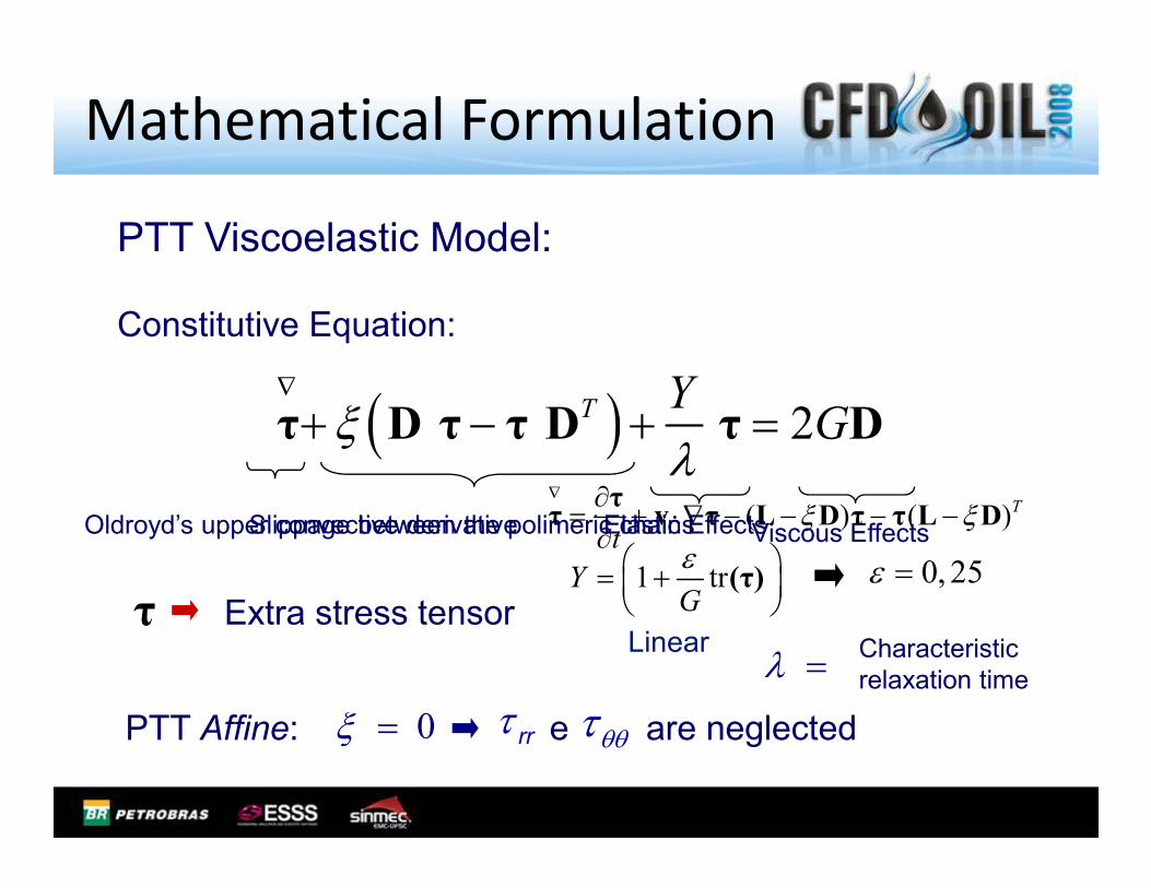
PTT Viscoelastic Model:

( ) 2T YGξ

λ

∇

+ − + =τ D τ τ D τ D� �

Constitutive Equation:

Mathematical Formulation

( ) 2Gξλ

+ − + =τ D τ τ D τ D� �

0ξ =

λ =Extra stress tensor

Oldroyd’s upper convective derivative ( ) ( )T

tξ ξ

∇ ∂= + ⋅∇ − − − −∂τ

τ v τ L D τ τ L DSlippage between the polimeric chainsElastic Effects

Characteristic

relaxation time

1 trYG

ε = +

(τ)

Viscous Effects

τ

τrr θθτ

0, 25ε =

Linear

PTT Affine: e are neglected

Mathematical formulation

• Governing equations

– Constitutive equations

2 2rr rr r r rr z rr rz rr

V V VYV V G

r z r z r

τ ττ τ τ

λ∂ ∂ ∂ ∂ ∂ + − + + = ∂ ∂ ∂ ∂ ∂

2 2r rr z

V VYV V G

r z r r

θθ θθθθ θθ

τ ττ τ

λ∂ ∂ + − + = ∂ ∂

2 2zz zz z z zr z zr zz zz

V V VYV V G

r z r z z

τ ττ τ τ

λ∂ ∂ ∂ ∂ ∂ + − + + = ∂ ∂ ∂ ∂ ∂

rz rz r z r z rr z zz rr rz rz

V V V V VYV V G

r z z r r r z

τ ττ τ τ τ

λ∂ ∂ ∂ ∂ ∂ ∂ + − + − + = + ∂ ∂ ∂ ∂ ∂ ∂

BSD Scheme (Phan-Thien et al., 2004):

( ) ( )ptρ ρ ρ

∂+ ∇ = −∇ +∇ +

∂v vv I τ g� � �

Introduces a diffusive term in both sides of

Mathematical Formulation

( ) ( ) ( )pt

η ηρ ρ ρ∂

+∇ = −∇ +∇ +∂

− ∇ − ∇v v v vv I τ g� � �

the momentum equation

The elliptic operator is amplified

reduction of the spurious oscilations

Mathematical formulation

• Conservation equations in the general form

( ) .( ) .( )u S Pρφ ρ φ φ∂

+∇ = ∇ Γ ∇ + +( ) .( ) .( )u S Pρ φφ φρ +∇ = ∇ Γ ∇ + +∂ ( ) . .() )( u S Pρ φφ ρ φ∂

+ = ∇ Γ ∇ + +∇( ) .( .( ))u S Pρφ ρ φ φ∇∂

+∇ = ∇ + +Γ( ) .( ) .( )u S Pρφ ρ φ φ∂

+∇ = ∇ ∇ + +Γ( ) .( ) .( )u S Pt

φ φ φρφ ρ φ φ+∇ = ∇ Γ ∇ + +∂( ) .( ) .( )u S Pt

φ φ φρ φφ φρ +∇ = ∇ Γ ∇ + +∂

Transient termConvective term

( ) . .() )( u S Pt

φ φ φρ φφ ρ φ+ = ∇ Γ ∇ + +∇∂

Diffusive term

( ) .( .( ))u S Pt

φ φφρφ ρ φ φ∇+∇ = ∇ + +Γ∂

Source terms

( ) .( ) .( )u S Pt

φ φφρφ ρ φ φ+∇ = ∇ ∇ + +Γ∂

Mathematical formulationEquations φ φΓ Sφ Pφ

Mass conservation

1 0 0 0

Momentum conservation in r direction

rV 0 ( )1

rr rzr

r r z r

θθττ τ∂ ∂

+ −∂ ∂

p

r

∂−∂

Momentum conservation in z direction

zV 0 ( )1

rz zzr

r r zτ τ

∂ ∂+

∂ ∂

p

z

∂−∂

z direction r r z∂ ∂ z∂

PTT component rr

rrτ

ρ 0 2 2r r rrr rr rz

V V VYG

r r zτ τ τ

λ∂ ∂ ∂ − + + ∂ ∂ ∂

0

PTT

component θθ θθτρ 0 2 2r r

V VYGr r

θθ θθτ τλ

− + 0

PTT component zz

zzτ

ρ 0 2 2z z zzz zr zz

V V VYG

z r zτ τ τ

λ∂ ∂ ∂ − + + ∂ ∂ ∂

0

PTT component rz

rzτ

ρ 0 z r r z r

rz zz rr rz

V V V V VYG

r z z r rτ τ τ τ

λ∂ ∂ ∂ ∂ + − + + − ∂ ∂ ∂ ∂

0

Numerical formulation

• System to be solve

– Equations

7 equations

7 variables

– Equations

• Mass conservation – 1 variable

• Momentum conservation – 2 variables

• Constituve equations (PTT) – 4 variables

– Variables: , , , , , ,r z rr zz rz zr

p V V θθτ τ τ τ τ=

Numerical solution

• PHOENICS CFD

– Finite Volume Method

– Staggered Grid– Staggered Grid

– Hybrid interpolation scheme

– SIMPLEST algorithm to solve pressure-velocity

coupling

– TDMA with under-relaxation factors

Results

Mesh

Test

200×200

Viscoelastic flow through a concentric annular

200×200

(De=50)

Shear stress profile, τrz

Viscoelastic flow through a concentric annular

1,0E-02

1,0E-01

erro médio (%)

PTT+BSD

PTT

1,00E-02

1,00E-01

erro médio (%)

PTT+BSD

PTT

Results

Average error (%)

1,0E-04

1,0E-03

100 1000 10000 100000

nº iterações

erro médio (%)

1,00E-04

1,00E-03

100 1000 10000 100000

nº iterações

erro médio (%)

Evolution of the percentage relative error during the monitoring of the

axial velocity convergence, with De = 100.

Evolution of the percentage relative error during the monitoring of the

axial velocity convergence, with De = 1.

Average error (%)

iterations

Results

Axial velocity profileAxial velocity profile

• Deborah number influence on the flow pattern�We were able to solve up to Deborah number 150.

� Results compared with Pinho and Oliveira (2000)

Results

• Deborah number influence on the flow pattern

Normal stress profileNormal stress profile

• Deborah number influence on the flow pattern

Results

Relative errors < 1%.

Shear rate dependent viscosityShear rate dependent viscosity

• The Fanning Friction Factor (200×200 non-uniform mesh)

Numerical results

Pinho and Oliveira (2000)

Results

Relative erros

about 0.15%

f Re

Conclusions

� It was created on the commercial software PHOENICS–CFD a structure to

support different differential viscoelastic constitutive equations;

� The structure developed allows other differential constitutive equations to be

easily implemented, making possible to utilize all the advantages of a

commercial software;

� The PTT viscoelastic differential model was implemented and solved for � The PTT viscoelastic differential model was implemented and solved for

axial flow through a concentric annular. The performance of the numerical

results obtained was excellent when compared with the analytical solution

available;

� The numerical convergence was drastically improved by employing the BSD

scheme. So the reductions in the computational efforts;

� In the future numerical simulation of the drilling fluid flow modeled as

viscoelastic could supply new information to improve de drilling fluid functions.

Next Steps

� Evaluate de influence of the non-linear Y function to represent the

extensional effects;

� Include the slippage between the molecular network and the

continuum medium;

� Implement the EVSS scheme (Rajagopalan, 1990);

� Simulate the axial and rotational movements of the drill column;

� Simulate the PTT viscoelastic fluid flow in geometries were the

convective and extensional effects are very important (contractions and

expansions), using the BSD and EVSS schemes.

Acknowledgments