Numerical Simulation of Internal Flow Field in Transonic Axial Compressor

Tao Ye1, a , Fei Chen2, b

1,2School of Mechanical and Electronical Engineering, WHUT, Wuhan 430070, China a whyetao@hotmail.com, bchenliaofei@126.com

Keywords: axial compressor; internal flow field; profile loss; numerical simulation; fitting Abstract: The transonic axial compressor Stage35 was selected as a research object, using software NUMECA taking numerical simulation of it. And then, the distribution rules of pressure and temperature of meridional channel and blade surface are derived. On this basis, the formation process of shock wave and the influence of it on boundary layer were analyzed in detail. Using the least square cubic fit method, the characteristic curve of the compressor was fitted. The analysis results indicate that the profile loss makes the energy loss of compressor remarkable add, and the characteristic curve can be fitted precisely by using the least square cubic fit method.

Introduction Turbine is one of the most important power equipments, which plays an important role in the

national economy and in the construction of national defense. It is divided into steam turbine, gas turbine, water turbine, fan and so on. The core machine of the gas turbine used in ship and aero-engine are both composed of compressor, combustion chamber and turbine. As one of the three core components, the compressor has a very important influence on the overall performance of gas turbines and aircraft engines. Therefore, in-depth study of the compressor in the internal flow mechanism [1] and energy loss mechanism [2] has double value of theory and applications.

At present, the main method on the research of compressor is numerical stimulation and experiment combined with numerical stimulation [3, 4]. Due to the limitation of experimental conditions, and the rapid development of computer technology, the computational fluid dynamics CFD method used in numerical simulation of the compressor internal flow field through computers can partly replace experiment, shorten the development period of the compressor and reduce the cost. In addition, the numerical simulation can provide a lot of flow field information, providing designers with some guidance in the subsequent design and optimization of compressor.

In this paper, the Stage35 transonic axial compressor is simulated and calculated, using Fine / Turbo software to earn detailed internal flow field under the design speed of the compressor which is specific for turbo-machinery. And then, the distribution rules of pressure and temperature of meridional channel and blade surface are derived, airfoil loss mechanism is analyzed and the characteristic curve of the compressor is fitted.

Meshing The transonic axial compressor Stage35 is selected as research object in this article,

three-dimensional model shown in Figure 1, the design parameters shown in Table 1. In this paper, the IGG / AutoBride modules of NUMECA software are used to divide mesh model, mesh topology using HOH structure, wherein inlet and outlet section of the flow channel with H-type mesh, blades fragments using O-grid. Calculation is based on the single cycle, which can greatly reduce the number of grids, accelerate the convergence speed, reduce the requirement of computer hardware and reduce the computation period. Single cycle blade grids are shown in figure 2. Using trebling grids, overall grids is 2322075, 1030291 grids for rotor, 1291784 for static blades, minimum orthogonality angle is 34.681 degrees, maximum aspect ratio is 1177.7, the maximum expansion ratio 1.867, the specific data as shown in table 2.

3rd International Conference on Mechatronics and Information Technology (ICMIT 2016)

© 2016. The authors - Published by Atlantis Press 371

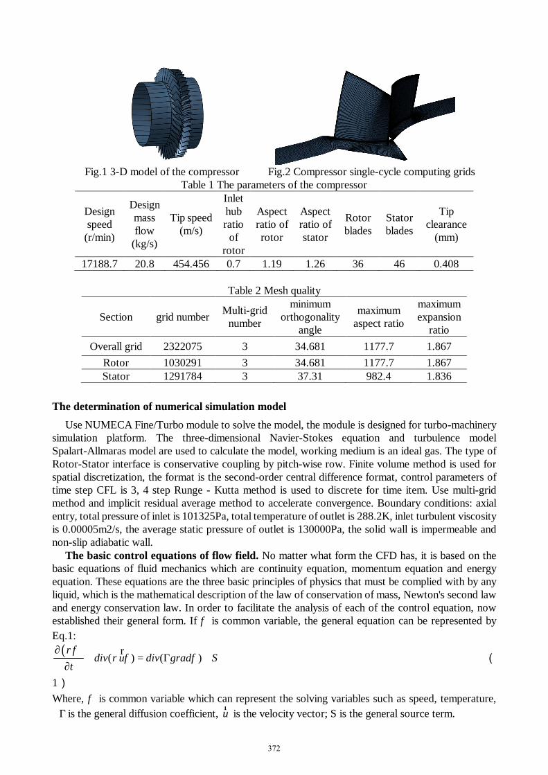
Fig.1 3-D model of the compressor Fig.2 Compressor single-cycle computing grids

Table 1 The parameters of the compressor

Design speed

(r/min)

Design mass flow

(kg/s)

Tip speed (m/s)

Inlet hub ratio

of rotor

Aspect ratio of rotor

Aspect ratio of stator

Rotor blades

Stator blades

Tip clearance

(mm)

17188.7 20.8 454.456 0.7 1.19 1.26 36 46 0.408

Table 2 Mesh quality

Section grid number Multi-grid number

minimum orthogonality

angle

maximum aspect ratio

maximum expansion

ratio Overall grid 2322075 3 34.681 1177.7 1.867

Rotor 1030291 3 34.681 1177.7 1.867 Stator 1291784 3 37.31 982.4 1.836

The determination of numerical simulation model Use NUMECA Fine/Turbo module to solve the model, the module is designed for turbo-machinery

simulation platform. The three-dimensional Navier-Stokes equation and turbulence model Spalart-Allmaras model are used to calculate the model, working medium is an ideal gas. The type of Rotor-Stator interface is conservative coupling by pitch-wise row. Finite volume method is used for spatial discretization, the format is the second-order central difference format, control parameters of time step CFL is 3, 4 step Runge - Kutta method is used to discrete for time item. Use multi-grid method and implicit residual average method to accelerate convergence. Boundary conditions: axial entry, total pressure of inlet is 101325Pa, total temperature of outlet is 288.2K, inlet turbulent viscosity is 0.00005m2/s, the average static pressure of outlet is 130000Pa, the solid wall is impermeable and non-slip adiabatic wall.

The basic control equations of flow field. No matter what form the CFD has, it is based on the basic equations of fluid mechanics which are continuity equation, momentum equation and energy equation. These equations are the three basic principles of physics that must be complied with by any liquid, which is the mathematical description of the law of conservation of mass, Newton's second law and energy conservation law. In order to facilitate the analysis of each of the control equation, now established their general form. If φ is common variable, the general equation can be represented by Eq.1:

( ) ( ) ( )div u div grad St

ρφρ φ φ

∂+ = Γ +

∂r （

1） Where, φ is common variable which can represent the solving variables such as speed, temperature,

Γ is the general diffusion coefficient, ur is the velocity vector; S is the general source term.

372

Turbulence Model. The Spalart-Allmaras turbulence model [5] is a one equation turbulence model which can be considered as a bridge between the algebraic model of Baldwin-Lomax and the two equation models. The main advantage of the Spalart-Allmaras model when compared to the one of Baldwin-Lomax is that the turbulent eddy viscosity field is always continuous. Its advantage over the k-ε model is mainly its robustness and the lower additional CPU and memory usage. Considering the advantages and characteristics of Spalart-Allmaras turbulence model, use the model to calculate in this paper. The principle of this turbulence model is based on the resolution of an additional transport equation for the eddy viscosity. The equation contains an advective, a diffusive and a source term and is implemented in a non conservative manner. The turbulent viscosity is given by

1t fνν ν= % （2） where ν% is the turbulent working variable and 1fν a function defined by

3

1 31

fcν

ν

χχ

=+

（

3）

with χ is the ratio between the working variable ν% and the molecular viscosityν , νχ

ν=

%

The turbulent working variable obeys the transport equation

( )( ){ }2 21 1 b bV c c Q

tν

ν ν ν ν ν νσ

∂ + ⋅∇ = ∇ ⋅ + + ∇ − ∇ + ∂

r%% % % % % （

4）

where Vr

is the velocity vector, Q the source term and, σ , 2bc constants. The source term includes a production term and a destruction term:

( )( )Q P Dν ν ν ν= −% % % % （

5）

Where, 1( ) bP c Sν ν ν=% % % （6）

( )2

1w wD c fdν

ν ν =

%% % （

7） The production term P is constructed with the following functions:

3 22 2S Sf fdν ν

νκ

= +%% （

8）

( )2 32

11 /

fcν

νχ=

+ （

9） ( ) ( )1 2

3

1 1f ff ν νν

χχ

+ −= （

10） where d is the distance to the closest wall and S the magnitude of vorticity.

373

In the destruction term (Eq. 7), the function wf is 1

6 63

6 63

1 ww

w

cf gg c

+= +

(11)

where，

( )62wg r c r r= + − (12)

2 2rS d

νκ

=%

% (13)

The constants arising in the model are ( )2

1 1 2/ 1 /w b bc c cκ σ= + + , 2 0.3wc = , 3 2wc = , 1 7.1vc = , 2 5vc = .

1 0.1355bc = , 2 0.622bc = , 0.41κ = , 2 / 3σ = . The equation Eq. 4 is solved with the appropriate boundary conditions:

On a solid wall 0ν =% , along the inflow boundaries the value of tν is specified (ν% is obtained by using a Newton-Raphson procedure to solve Eq. 2) and along the outflow boundaries it is extrapolated from the interior values.

Calculation results and analysis

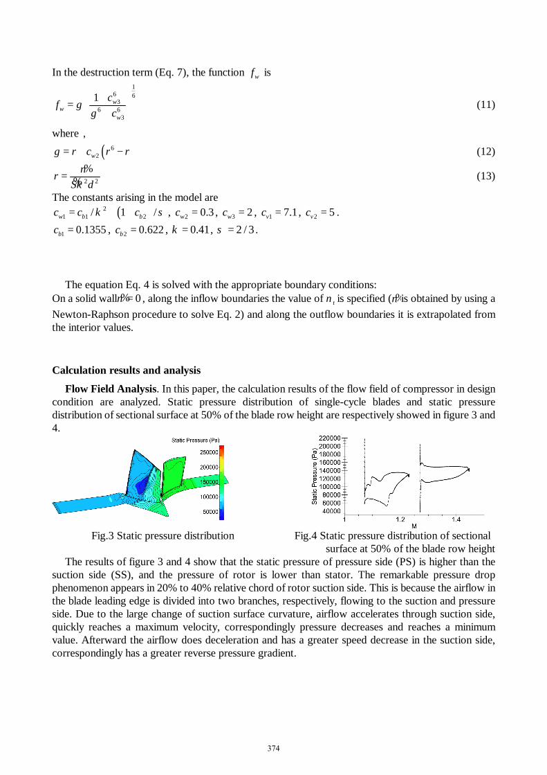
Flow Field Analysis. In this paper, the calculation results of the flow field of compressor in design condition are analyzed. Static pressure distribution of single-cycle blades and static pressure distribution of sectional surface at 50% of the blade row height are respectively showed in figure 3 and 4.

Fig.3 Static pressure distribution Fig.4 Static pressure distribution of sectional

surface at 50% of the blade row height The results of figure 3 and 4 show that the static pressure of pressure side (PS) is higher than the

suction side (SS), and the pressure of rotor is lower than stator. The remarkable pressure drop phenomenon appears in 20% to 40% relative chord of rotor suction side. This is because the airflow in the blade leading edge is divided into two branches, respectively, flowing to the suction and pressure side. Due to the large change of suction surface curvature, airflow accelerates through suction side, quickly reaches a maximum velocity, correspondingly pressure decreases and reaches a minimum value. Afterward the airflow does deceleration and has a greater speed decrease in the suction side, correspondingly has a greater reverse pressure gradient.

374

(a) contour (b) curve graph

Fig.5 Static temperature distribution of meridional flow channel

(a) contour (b) curve graph

Fig.6 Static pressure distribution of meridional flow channel Static temperature and static pressure distribution of meridional flow channel are respectively

showed in figure 5 and 6. Static temperature and static pressure distribution curve graph of the midst of meridional flow channel are respectively showed in (b) of figure 5 and 6. The results indicate that temperature and pressure is on the rise tendency as a whole along the meridional channel. Due to the wave resistance loss, the temperature and pressure at the leading edge drop to a minimum value. And temperature and pressure sharply rise when airflow through rotor. Because of the wake loss near the trailing edge of rotor blades and wave resistance loss at the leading edge of stator blades, temperature and pressure decrease in the Rotor-Stator interface. At the trailing edge of stator, temperature and pressure reach to the maximum value, and then decrease slowly and stabilize to a certain value.

(a) Static temperature distribution (b) Static pressure distribution

Fig.7 Static temperature and pressure distribution of blade leading and trailing edge along span Static temperature and static pressure distribution of blade leading and trailing edge along span are

showed at figure 7. The results of figure 7 show that temperature gradually increases along span at the leading and trailing edge of rotor. This is because the rotor speed increases gradually along the span, and the friction between blades and air is more and more intense, resulting in temperature rising. However, the temperature of stator has a relatively uniform distribution along span, only a little rise near the root and tip of blades because of the friction between airflow and boundary layer, causing friction loss. The results of figure 7 indicate that pressure gradually increases along span at the leading edge of rotor, while it changes rarely at the trailing edge. The pressure of stator has a relatively uniform distribution along span.

375

Fig.8 Relative Mach Number of S1 flow Fig.9 An enlarged view of Ⅰ

surface at 50% of the blade row height

Fig.10 An enlarged view of Ⅱ Fig.11 The corresponding velocity vector of Ⅰ

Relative Mach number of S1 flow surface at 50% of the blade row height, enlarged view of Ⅰ and

Ⅱ are respectively showed at figure 8, 9 and 10. The results show that in the inlet section, the airflow is supersonic flow, and in the outlet section, the airflow is subsonic flow. And the relative Mach number gradually reduces from inlet to outlet. Overall, airflow has a tendency of velocity decrease and pressure increase. Shock wave is formed by supersonic airflow at the blade leading edge, after that the airflow is subsonic, and then the airflow is divided into two at stagnation point, flowing to the pressure side and suction side respectively. Airflow along the suction side reaccelerates to supersonic flow when it goes through the leading edge and the suction side, forming expansion wave which interferes with the boundary layer and leads to the separation of boundary layer and the formation of eddy, which causes greatly energy loss. The acceleration process of airflow along the suction side is showed in figure 11 in detail.

Fitting characteristic curve. The requirement of computer for the numerical calculation of compressor is very higher, and the computation takes a long time. In order to get the compressor characteristic curve, a large number of lengthy interpolations are still needed. Use the least square cubic fit method which references Zhang Dongyang [6] and Liu xiaofang [7] provided methods, to fit out compressor characteristic curve of mass flow-efficiency and mass flow-pressure ratio under the design rotating speed 17188.7 r/min in this paper, as shown in figure 12 and 13.

Fig.12 Mass flow-efficiency curve Fig.13 Mass flow-pressure ratio curve

376

Conclusions 1. The analysis results of internal flow field of compressor indicate that the velocity of airflow

decreases, the pressure and temperature increase along axial direction. And in spanwise direction, the pressure and temperature of rotor blades change a little large, but the pressure and temperature of stator blades change little, only some fluctuations near the root and tip of stator blades.

2. Airfoil loss of transonic compressor comprises friction loss caused by the friction between airflow and boundary layer, separation loss caused by the separation and vortex of boundary layer gas, wake loss caused by boundary layer air converging at the trailing edge of blades and wave resistance loss caused by supersonic airflow, which leads to remarkable energy loss.

3. The compressor characteristic curve can be fitted by the least square cubic fit method which has high fitting precision and wide engineering application prospects.

References [1] L.M Gao, X Chen, Y Bai, X.D Feng. Numerical simulation of 3-D viscous flow field in a axial compressor stage[J]. Chinese Journal of Mechanics, 2013,04:569-573+448-649. [2] X.F Wang, P.G Yan, L.B Yu, W.J Han. Separated vortex flow of inner flow field in two-stage axial compressor[J]. Acta Aerodynamica Sinica, 2014,02:177-183+202. [3] X Gao, W.L Chu. Numerical studies of non-axisymmetric endwall molding for transonic axial compressor rotor [J]. Fluid Machinery, 2013,08:35-39. [4] Natalie R. Smith, Nicole L. Key. Flow visualization for investigating stator losses in a multistage axial compressor[J]. Exp Fluids (2015) 56:94. [5] Spalart P R, Allmaras S R. A One-Equation Turbulence Model for Aerodynamic Flows[J]. La Recherche Aérospatiale, 1992, 439(1):5-21. [6] Zhang Dongyang. Fitting method of Compressor performance coefficient[J]. Gas Turbine Technology, 1993,6(3):27-32. [7] X.F Liu, L Jiang, P.S Si, J.K Zhang. Characteristic curve fitting method for gas turbine compressor[J]. Ship Science and Technology,2012,07:61-63.

377