1

Numerical Simulations of Optical Turbulence Using an Advanced Atmospheric Prediction Model: Implications for Adaptive Optics Design

Randall J. Alliss and Billy D. Felton Northrop Grumman Information Systems

7555 Colshire Dr McLean, VA 22102

Abstract Optical turbulence (OT) acts to distort light in the atmosphere, degrading imagery from astronomical telescopes and reducing the data quality of optical imaging and communication links. Some of the degradation due to turbulence can be corrected by adaptive optics. However, the severity of optical turbulence, and thus the amount of correction required, is largely dependent upon the turbulence at the location of interest. Therefore, it is vital to understand the climatology of optical turbulence at such locations. In many cases, it is impractical and expensive to deploy instrumentation to characterize the climatology of OT for a given location, so numerical simulations become a convenient and less expensive alternative. The strength of OT is characterized by the refractive index structure function Cn

2, which in turn is used to calculate atmospheric seeing parameters. While attempts have been made to characterize Cn

2 using empirical models, Cn2 can be calculated more directly from Numerical Weather Prediction

(NWP) simulations using pressure, temperature, thermal stability, vertical wind shear, turbulent Prandtl number, and turbulence kinetic energy (TKE). In this work, the Weather Research and Forecast (WRF) NWP model is used to generate Cn

2 climatologies in the planetary boundary layer and free atmosphere, allowing for both point-to-point and ground-to-space seeing estimates of the Fried Coherence length (r0) and other seeing parameters. Simulations are performed on a multi-node Linux cluster using the Intel chip architecture. The WRF model is configured to run at 1-km horizontal resolution over a domain that includes the Mauna Loa Observatory (MLO) of the Big Island and Haleakala on Maui. The vertical resolution varies from 50 meters in the boundary layer to 500 meters in the stratosphere. The model top is 20 km. The Mellor-Yamada-Janjic (MYJ) TKE scheme has been modified to diagnose the turbulent Prandtl number as a function of the Richardson number, following observations by Kondo and others. This modification de-weights the contribution of the buoyancy term in the equation for TKE by reducing the ratio of the eddy diffusivity of heat to momentum. This is necessary particularly in the stably stratified free atmosphere where turbulence occurs in thin layers not typically resolvable by the model. The modified MYJ scheme increases the probability and strength of TKE in thermally stable conditions thereby increasing the probability of optical turbulence. Nearly two years of simulations have been generated. Results indicate realistic values of r0 are obtained when compared with observations from a Differential Image Motion Monitor (DIMM) instrument. Seeing is worse during day than at night with large values of r0 observed just after sunset and just before sunrise. Three-dimensional maps indicate that the vast lava fields present on the Big Island have a large impact on turbulence generation. Results from this study are being used to make design decisions for adaptive optics systems. Detailed results of this study will be presented at the conference.

2

1. Introduction

With High Performance Computing (HPC) platforms becoming much more affordable and accessible, simulations of physical parameters in the atmosphere are easily performed. In this work, HPC is used to simulate free space optical turbulence (OT) for an extended time period at very high resolution. OT has long been an important atmospheric phenomenon for astronomers because of the impact it has on atmospheric seeing, and it is becoming increasingly important for communications engineers. Small-scale temperature and moisture fluctuations in the atmosphere result in fluctuations of the refractive index. The wave front of radiation traveling through the atmosphere changes as it encounters inhomogeneities in the refractive index, degrading optical image quality. The intensity of the turbulent fluctuations of the atmospheric refractive index is described by the refractive index structure function, Cn

2. The ability to quantify the OT above an observatory and to understand its vertical distribution is vital, and can impact decisions on adaptive optics design, observatory scheduling, and site selection for new observatories. Similarly, the optical turbulence characteristics of potential optical communications ground station locations influence link budgets and other aspects of the system design. Although instruments have been developed to characterize OT, they are expensive to deploy and maintain over long periods of time and the quality of the data is limited.

Numerical simulations of OT are an attractive alternative to local observations in regions where infrastruc-ture (e.g. electrical power) is lacking. Numerical simulations offer many advantages over direct measurements. These advantages include having a three-dimensional description of Cn

2 over regions of interest, simulations that can be performed anywhere on earth at any time, and the ability to provide forecasts of OT that can be used for observational scheduling purposes. The OT numerical simulations for this study are performed by a computer model used to predict tropospheric weather. The meteorological community refers to such models as Numerical Weather Prediction (NWP), and routinely uses them to predict everyday weather. However, for this application, an NWP model is modified and run at very high resolution to make simulations of Cn

2. The reliability of these types of simulations for describing the climatology of OT has been shown to be quite good. These simulations have been used to support NASA with site characterization, site selection, and system design studies for its recent Lunar Laser Communications Demonstration (LLCD) and upcoming Laser Communications Relay Demonstration (LCRD). In this paper we describe how NWP is leveraged to simulate OT, and we present various results along with comparisons to direct observations of integrated OT.

2. Technical Approach

In this study we use version 3.2 of the Weather Research and Forecasting (WRF) model developed jointly by the National Center for Atmospheric Research (NCAR) and the National Oceanic and Atmospheric Administration (NOAA) (Skamarock et al., 2008). WRF is a mesoscale NWP model developed for the prediction of weather and is routinely used by the National Weather Service and other forecasting services. The model is based on the Navier-Stokes equations, which are solved numerically on a three-dimensional grid. The model simulates four basic atmospheric properties: wind, pressure, temperature, and atmospheric water vapor. All others variables are derived from these four.

This study uses the WRF model to characterize the climatology of OT over the Hawaiian Islands including the summits on Maui and the Big Island. Several aspects of the OT are examined, including its diurnal cycle and variations with terrain elevation and land usage. The following sections describe the model setup, modifications to the code, derivation of OT parameters, and results of simulations to date. a. Model Setup

WRF is used to simulate daily meteorological conditions for Hawaii for 20 months during the years of 2009, 2013, and 2014. The model is configured at 1-km horizontal resolution with dimensions of 272x272 grid points and 83 vertical levels. The resolution of the vertical levels is approximately 50-100 m below 2 km above ground level (AGL), 150-250 m for 2–13 km AGL, and 500 m up to the model top (50 millibars, approximately 20km). Simulations are initialized at 1200 UTC directly from the 0.5° Global Forecasting System (GFS) analysis produced by the National Weather Service. Lateral boundary conditions are provided out to 27 hours by three-hourly GFS forecasts. This allows for filtering out model “spin-up” by excluding the first three simulation hours, while still

3

capturing the full 24-hour diurnal cycle. Selected physics and diffusion options are summarized in Table 1. The model was reinitialized each day during the simulation period.

Table 1. Physics and diffusion settings used in WRF model for this study

Time Integration RK3 Time Step 2 sec Horizontal/Vertical Advection Fifth/Third order Explicit Diffusion Physical space 2D deformation, no sixth order Boundary Layer Physics Mellor, Yamada, Janjic (MYJ) Surface Layer Janjic Eta Land Surface Noah Shortwave/Longwave Radiation Dudhia/RRTM Microphysics WSM6 Cumulus Parameterization None

b. Model Modifications

The minimum turbulence kinetic energy (TKE) permitted in the Mellor-Yamada-Janjic (MYJ) scheme had to be modified. The default setting gives TKE values >0.1 m2s–2, resulting in unrealistically large values of Cn

2 in the free atmosphere. Following Gerrity et al. (1994), the minimum TKE limit was changed to 10–5 m2s–2. The second modification involves the eddy diffusivities of heat and momentum (KH and KM, respectively). In the original MYJ scheme, these variables are given by

Where is the mixing length, and and are functions of TKE, mixing length, buoyancy,

and vertical wind shear (Mellor and Yamada, 1982). In the modified version these relationships are unchanged for neutral and unstable conditions. However, when the gradient Richardson number (Ri) is greater than 0.01, an implementation by Walters and Miller (1999) is followed whereby is adjusted according to:

The equation was first proposed by Kondo et al. (1978). The Kondo equation decreases with increasing

Ri, effectively increasing the TKE production by vertical wind shear. This is necessary to generate free atmospheric turbulence that is commonly associated with jet streams. Without this change, the model rarely produces TKE larger than the model’s minimum value, something that is considered unrealistic when compared to many global thermosonde measurements (Ruggiero, personal communication, 2008).

,, MqhHqh SlKSlK ==

l ,2TKEq = ,HS ,MS

MK

⎪⎪⎪

⎩

⎪⎪⎪

⎨

⎧

≤<

++

≥=

.101.0

873.611873.6

1

,1,7

1

Rifor

RiRi

forRiRi

KKM

H

KH

KM M

H

KK

4

Improvements to the land usage modeling have been made for the Hawaiian domain. In the original research, we used a very simple land usage dataset that did not accurately represent the true land usage. This dataset over-estimated the amount of lava rock present on the islands. The result of this over-estimate yielded surface heat fluxes that were too strong and thus over-estimated the severity of turbulence. Figure 1a shows the original land usage dataset, and 1b its recent replacement. Note the higher level of detail in Figure 1b. This has a measurable impact on the quality and accuracy of the optical turbulence simulations.

Figure 1a. Original land usage data. Figure 1b. Improved land usage data.

c. Derivation of Seeing

The seeing parameters of interest to astronomers and optical communications system designers can be derived from the refractive index structure function, Cn

2. When turbulence is locally homogeneous and isotropic, Cn2

is related to changes in the refractive index. Large values of Cn2 correspond to increasing changes in the refractive

index and thus greater turbulence. Tatarskii (1971) derived an alternative expression for the structure function parameter applicable for optical wavelengths:

where P is atmospheric pressure, T is air temperature, and is the structure function parameter for temperature.

is given by:

where is an empirical constant, is the outer length scale of turbulence (i.e., the upper bound of the inertial

subrange), and is the vertical gradient of potential temperature. Following Walters and Miller (1999), is set

to 2.8 and calculation of the outer length scale of turbulence in the thermally stable conditions is approximated from Deardorff (1980):

22

2

82 1079

Tn CT

PC ⎟⎟⎠

⎞⎜⎜⎝

⎛ ∗=

−

2TC

2TC

234

22 ⎟⎠

⎞⎜⎝

⎛∂∂

⎟⎟⎠

⎞⎜⎜⎝

⎛=

ZL

KKaC oM

HT

θ

2a oL

∂θ∂Z"

#$

%

&'

2a

Based on landsat data

5

where N is the Brunt-Vaisala frequency. In thermally unstable conditions, is related to the depth of the unstable boundary layer.

In this study, we also compute the Fried coherence length, r0, which is a measure of phase distortion of an optical wave front by turbulence. This parameter represents the integrated effect of turbulence along a line of sight, and can vary rapidly over time and from one point of the sky to another. Larger values of r0 are indicative of less turbulence and better seeing, while smaller values of r0 represent stronger turbulence and worse seeing. The coherence length (Fried, 1965) is calculated by integrating Cn

2 along a path, z:

3. Results

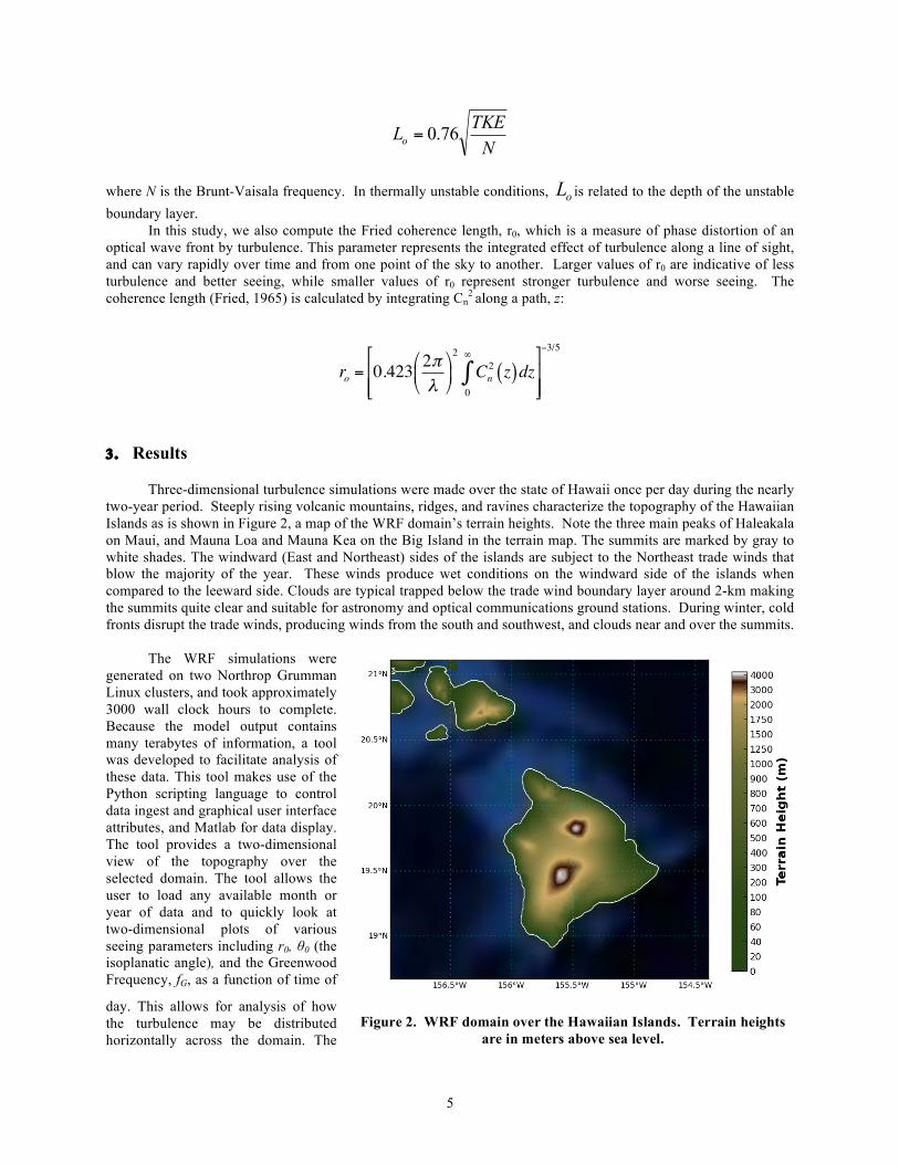
Three-dimensional turbulence simulations were made over the state of Hawaii once per day during the nearly two-year period. Steeply rising volcanic mountains, ridges, and ravines characterize the topography of the Hawaiian Islands as is shown in Figure 2, a map of the WRF domain’s terrain heights. Note the three main peaks of Haleakala on Maui, and Mauna Loa and Mauna Kea on the Big Island in the terrain map. The summits are marked by gray to white shades. The windward (East and Northeast) sides of the islands are subject to the Northeast trade winds that blow the majority of the year. These winds produce wet conditions on the windward side of the islands when compared to the leeward side. Clouds are typical trapped below the trade wind boundary layer around 2-km making the summits quite clear and suitable for astronomy and optical communications ground stations. During winter, cold fronts disrupt the trade winds, producing winds from the south and southwest, and clouds near and over the summits.

The WRF simulations were

generated on two Northrop Grumman Linux clusters, and took approximately 3000 wall clock hours to complete. Because the model output contains many terabytes of information, a tool was developed to facilitate analysis of these data. This tool makes use of the Python scripting language to control data ingest and graphical user interface attributes, and Matlab for data display. The tool provides a two-dimensional view of the topography over the selected domain. The tool allows the user to load any available month or year of data and to quickly look at two-dimensional plots of various seeing parameters including r0, θ0 (the isoplanatic angle), and the Greenwood Frequency, fG, as a function of time of

day. This allows for analysis of how the turbulence may be distributed horizontally across the domain. The

NTKELo 76.0=

oL

ro = 0.423 2πλ

!

"#

$

%&2

Cn2 z( )dz

0

∞

∫)

*++

,

-..

−3/5

Figure 2. WRF domain over the Hawaiian Islands. Terrain heights are in meters above sea level.

6

user may also look at the distribution of any of these parameters for a single vertical column in the domain. The Mauna Loa Observatory (MLO) is the main focus in this study due to the interest of NASA in

establishing an optical ground station there. Characterizing and understanding the weather and turbulence at MLO are vital to the ultimate design and operation of the ground station. While the summit of Mauna Loa reaches 13,678 feet above sea level, MLO is located on the north slope of the mountain, about 2500 feet below the summit. Consequently, it suffers somewhat more cloud cover due to the fact that its lower elevation allows the boundary layer clouds to obscure MLO more frequently. However, it is also less exposed to the harsh temperatures and winds present at the summits of Mauna Loa and Mauna Kea. These results examine the effects of location, time of day, and winds on the turbulence of MLO, and compare MLO to other potential locations in Hawaii.

The cumulative distributions of r0 for MLO derived from the WRF simulations are shown in Figure 3. The values shown only represent the times when WRF shows the site to be cloud-free, i.e. times where the total cloud liquid water and ice water content are very near zero. MLO exhibits a large difference between the values of r0 during the daytime and those simulated during the nighttime hours. The plot shows the median overall value of r0 is 13.1 cm, while the daytime and nighttime median values are 8.1 cm and 22.1 cm, respectively. This is the expected behavior for most locations over land, since daytime heating of the land creates thermal instability and drives the creation and maintenance of strong atmospheric turbulence. At night the land cools, the lower atmosphere becomes thermally stable, and turbulence is suppressed. The degree to which this happens and the relative strengths of daytime and nighttime turbulence varies by location, governed by phenomena such as surface heat capacity, elevated nocturnal temperature inversions, and wind speed.

Figure 3. Cumulative distributions of r0 for

MLO for all times (black), day (red), and night (blue). Values of r0 are referenced to

500 nm and zenith.

Figure 4. Median hourly r0 for MLO with the

5% and 95% data intervals shown by the vertical bars.

The diurnal variation of r0 at MLO is clearly observed in Figure 4. In this plot, the line that connects the

vertical bars shows the median value of r0 for each hour of the day. The vertical bars show the range of 90% of the data for each hour, from the 5% value at the bottom to the 95% value at the top of each bar. The values of r0 decrease rapidly after sunrise (~1700 UTC, 7 AM local), reach their minimum near and just after local noon (2200 UTC), and rise in the late afternoon maintaining large values throughout the night. The data indicate r0 is consistently between about 4 cm and 10 cm during mid-day and early afternoon hours when the surface heating is at its maximum. The seeing is much better during the nighttime hours, but the 5% values show there are times where the seeing is quite poor at night. Figure 5 is a two-dimensional histogram of r0 and wind speed that shows when the nighttime r0 value is less than 8 cm, the wind speed is usually greater than 6 m/s (approximately 12 knots). This is consistent with observations from Bradley et al. 2006 that show a correlation of r0 with wind speed.

7

For comparison, the r0 distributions for the

summit of Mauna Loa are shown in Figure 6 and Figure 7. While the median r0 at the summit during the day is very similar to MLO, the nighttime values are significantly smaller (worse) at the summit than at MLO. Similarly, the daytime distribution is much steeper at the summit than at MLO, showing that very good seeing conditions are more common below the summit than on the summit itself. This difference in r0 is shown spatially in the map of the mean values of nighttime r0 at (4:00 am HST) in Figure 8 where the most benign turbulence is observed near, but below, the summits of Mauna Loa and Mauna Kea at night. This may seem at odds with the traditional understanding that the most optimal seeing is located at the top of tall, isolated summits. The difference between the summits and the surrounding slopes is not as drastic in the daytime, implying WRF is simulating something during the night that often prevents the full suppression of turbulence at the highest elevations. One possible explanation for this is wind speed.

Figure 6. Cumulative distributions of r0 for the summit of Mauna Loa for all times (black), day (red), and night (blue). Values of r0 are referenced to 500 nm and zenith.

Figure 7. Median hourly r0 for the summit of Mauna Loa with the 5% and 95% data intervals shown by the vertical bars.

Figure 5. Two-dimensional histogram showing the frequency of occurrence of r0 and wind speed.

8

Figure 8. Mean values of r0 during the night (upper left, 0400 HST), sunrise (upper right, 0700 HST), day

(lower left, 1300 HST), and evening (lower right, 1900 HST). Values of r0 are referenced to 500 nm and zenith.

The WRF simulations indicate surface

winds are stronger at the summits of Mauna Loa and Mauna Kea compared to elevations slightly below the peaks. Figure 9 shows a map of the mean wind speed over the Big Island at night (0400 HST). There is a minimum in wind speed (dark blue color) immediately to the leeward (west) side of each of the peaks, as well as smaller areas of lighter wind on their windward sides. Note these areas of light mean wind speed during the night correspond to the same ring-shaped areas of the largest r0 on the slopes surrounding the Mauna Loa and Mauna Kea summits. It is postulated that the better seeing produced in the WRF simulations below summit level is an effect of mountain blocking, the result of which is quiet areas in the wind shadows of the peaks. While strong winds do not necessarily produce optical turbulence, strong winds near the ground produce wind shear, one of the generators of turbulence. If true, this information could prove valuable to astronomers and optical system designers. Unfortunately, at present, we know of no in-situ turbulence observations in these areas to corroborate these findings.

As mentioned previously, Cn2 is computed for every three-dimensional grid point in the WRF domain. From

this data, profiles of Cn2 can be extracted for any line-of-sight within the domain. Figure 10 and Figure 11 show the

WRF-derived mean vertical Cn2 profiles for five locations in the Hawaiian Islands for early afternoon (1400 Local

Figure 9. Mean wind speed (kts) at 10 meters above the ground during the night (left, 0400 HST) from WRF simulations.

9

Time) and overnight (0400 Local Time). Each Cn2 profile starts at ground level, and continues vertically to the top

of the WRF domain. Although the maximum values of the Cn2 profiles for each site differ near the surface, they all

show a deeper turbulent boundary layer in the daytime than at night. The MLO average profile, shown by the blue line, has the most shallow and benign nighttime Cn

2 between the surface and the free atmosphere. The profiles of the summits of Mauna Kea (green line) and Mauna Loa (orange line) are very similar during both night and day, and both have more intense Cn

2 than MLO. For comparison to the high-altitude sites, the black lines in the two plots show the profile above a location on the west coast of the Big Island near Kona. The average height of the top of the trade wind inversion is evident at about 2 km in the Kona Cn

2 profile where the non-surface layer Cn2 reaches its

maximum value. As expected, all five profiles are similar in the free atmosphere above about 4000-5000 meters, farther away from the effects of terrain and other surface characteristics.

Figure 10. Average Cn

2 profile for five locations in Hawaii in the early afternoon at

14:00 Local Time (0000 UTC).

Figure 11. Average Cn

2 profile for five locations in Hawaii overnight at 04:00 Local

Time (1400 UTC).

Turbulence measurement campaigns are generally limited to existing or potential astronomical observatories. Ideally, the r0 values from the WRF simulations would be compared to in situ data from MLO. However, there is no such data from MLO for comparison. Instead, turbulence data is available from field campaigns for Mauna Kea and Haleakala. The data available from the Thirty Meter Telescope (TMT) campaign was collected at night on a site near the summit of Mauna Kea (Skidmore et al, 2009). TMT conducted a multiyear field campaign from 2005-2008 to determine the most appropriate sites for the first generation of extremely large telescopes (ELTs). Mauna Kea was a field campaign site, and was ultimately selected as the preferred site for the TMT. In the campaign, astronomical seeing parameters were measured with a combined Differential Image Motion Monitor (DIMM) and Multi Aperture Scintillation Sensor (MASS). The cumulative distribution of the TMT r0 is shown by the blue line in Figure 12, and has a median r0 of about 13.5 cm. The red

Figure 12. Cumulative distributions of r0 for the summit of Mauna Kea at night from TMT

measurements (blue) and WRF (red and green). Values of r0 are referenced to 500 nm and zenith.

10

line shows the WRF-derived r0 distribution for the same location on Mauna Kea for all cloud-free times. The median r0 value from the WRF simulations is 12.5 cm. Although the median values from WRF and the TMT measurements are very close, the distributions diverge at smaller and larger values. One possible explanation of this may be that field campaigns often do not collect measurements during high wind conditions, whereas WRF computes a value for r0 at all times. When times at which the WRF 10m wind speed is greater than 30 kts are excluded from the distribution, the agreement between WRF and the TMT measurements improves in the lower half of the distributions. The medians are nearly identical, and the remaining values are within about 1 cm. However, the r0 values in the upper half of the WRF distribution in both cases are larger than the TMT measurements, though their maximum values are the same. Large (benign) values of r0 result from a very quiet atmosphere. In the WRF simulations, the TKE floor value within the model dictates the maximum value of r0 (i.e. the minimum Cn

2 profile). For these simulations, a background TKE profile prescribed by Masciadri (2009) is used to compute the values of Cn

2 (and thus r0) when the atmosphere is essentially non-turbulent. It is encouraging that WRF appears to accurately identify the probability of very good seeing conditions, despite over-estimating the values somewhat. In our opinion, quantifying the precise values of r0 during benign events is less essential to characterizing a site than quantifying how often very good seeing conditions occur.

As indicated earlier, optical communication engineers are using optical turbulence data to estimate its impact on performance. Along with cloud-free statistics, it is a main factor that may influence site selection for an optical down link. In previous work for the NASA LLCD mission, WRF was used to characterize the turbulence at several sites including Haleakala, Dryden, CA, Table Mountain, CA, and White Sands, NM. Results indicated that Haleakala has the most benign turbulence when compared with the other three sites. Currently NASA is interested in comparing different sites on the islands of Hawaii. Figure 13 shows the diurnal variation of r0 at Mauna Loa, Mauna Kea, and Haleakala. WRF indicates MLO has the best nighttime seeing of the three locations shown, but it also has the largest diurnal range with the worst values of r0 during the daytime. As discussed previously, it is hypothesized that this is related to calm winds below the summit created by terrain blocking. While optical turbulence has been measured over a reasonably long time period at both Haleakala and the summit of Mauna Kea, as of now, these WRF simulations provide the best estimate of seeing conditions at MLO. Future plans of NASA may include a turbulence monitor at MLO that can be used to corroborate this phenomenon.

4. Summary and Conclusions

Optical turbulence statistics for the Hawaiian Islands have been generated using a modified version of the WRF numerical weather prediction model. Results show WRF is able to produce realistic diurnal variations of optical turbulence as represented by the Fried coherence length, r0. A comparison to turbulence measurements from the TMT field campaign shows a similar distribution. These results indicate WRF is able to describe the climatology of optical turbulence over regions of interest, making the model a convenient tool to use to characterize turbulence over areas where observations are difficult to obtain. The WRF simulations also indicate that atmospheric seeing may be best a few hundred meters below the summits of Mauna Loa and Mauna Kea at night, instead of on the summits themselves. This interesting result needs to be tested against observations to be proven, but could be important to future site considerations. NASA has used these simulations of optical turbulence in its recent optical communications design and site selection studies.

Figure 13. Median hourly r0 for the MLO (blue), Mauna Kea summit (green), and Haleakala (red) with the 5% and 95% data intervals shown by the

vertical bars.

11

References Alliss, R.J and B.D. Felton, 2009: "Validation of Optical Turbulence Simulations from a Numerical Weather Prediction Model in Support of Adaptive Optics Design”, Advance Maui Optical and Space Surveillance Technologies Conference, Vol 1, p. 54. ATST Site Survey Working Group Final Report, 2004: http://atst.nso.edu/files/docs/RPT-0021.pdf Bradley, E.S., L.C. Roberts, L. W. Bradford, M. Skinner, D.A. Nahrstedt, M.F. Waterson and J.R. Kuhn, 2006: Characterization of Meteorological and Seeing Conditions at Haleakala. Publications of the Astronomical Soc. of the Pacific, 118:172-182. Deardorff, J. W., 1980: Stratocumulus-capped mixed layers derived from a three-dimensional model. Bound.-Layer Meteor., 18, 495–527.

Fried, D. L., 1965: Statistics of a geometric representation of wavefront distortion. J. Opt. Soc. Amer., 55, 1427–1435. Gerrity, J. P., T. L. Black, and R. E. Treadon, 1994: The numerical solution of the Mellor-Yamada level 2.5 turbulent kinetic energy equation in the Eta model. Mon. Wea. Rev., 122, 1640–1646.

Kondo, J., O. Kanechika, and N. Yasuda, 1978: Heat and momentum transfers under strong stability in the atmospheric surface layer. J. Atmos. Sci., 35, 1012–1021.

Masciadri, 2009. Book on Seeing, Ed. Institute for Astronomy, Hawaii, US.

Mellor, G. L., and T. Yamada, 1982: Development of a turbulence closure model for geophysical fluid problems. Rev. Geophys. Space Phys., 20, 851–875.

Skamarock, W. C., J. B. Klemp, J. Dudhia, D. O. Gill, D. M. Barker, M. G. Duda, X.-Y. Huang, W. Wang, and J. G. Powers, 2008: A description of the advanced research WRF version 3. NCAR Technical Note, NCAR/TN-475+STR, 113 pp.

Skidmore, W., E. Sebastian, T. Travouillon, R. Riddle, M. Schöck, E. Bustos, J. Seguel, D. Walker, 2009, “Thirty Meter Telescope Site Testing V: Seeing and Isoplanatic Angle”, Pub. Astr. Soc. of the Pac., 121:1151-1166.

Tatarskii, V. I., 1971: The effects of the turbulent atmosphere on wave propagation. Technical Report, U.S. Department of Commerce, NTIS TT-68-50464, 472 pp.

Walters, D. L., and D. K. Miller, 1999: Evolution of an upper-tropospheric turbulence event—comparison of observations to numerical simulations. Preprints, 13th Symposium on Boundary Layer Turbulence, AMS, 157–160, Dallas, TX.