numerical solution and stability analysis …internationalejournals.com/pdfs/ijmtah/ijmtah...

ISSN-2249 5460

Available online at ww.internationaleJournals.com

International eJournals

International Journal of Mathematical Sciences,

Technology and Humanities 120 (2014) 1285 - 1296

NUMERICAL SOLUTION AND STABILITY ANALYSIS OF A CLASS

OF THIRD ORDER DIFFERENTIAL EQUATIONS

C. Bala Rama Krishna1, P. Sunitha2, S. Vishwa Prasad Rao3 and P. S. Rama Chandra Rao4

1Department of Mathematics,

Chaitanya Degree College (Autonomous), Hanamkonda, Warangal - 506001, (A. P.), India.

[email protected]

2, 4

Department of Mathematics,

Kakatiya Institute of Technology & Science, Warangal - 506015, (A. P.), India.

[email protected], [email protected]

3Department of Mathematics,

Wollega University, Ethiopia, Africa. [email protected]

Abstract

In this paper, we have discussed solution and stability analysis of a class of third order

boundary value problem. We have solved a linear third order differential equation by using

our method. It has been noticed that the solution obtained by our method is very nearer to the

original solution

AMS Subject Classification: 65L05, 65L06

Keywords: Numerical differentiation; Boundary Value Problem; Absolute stability,

Multistep methods.

mailto:[email protected]




International Journal of Mathematical Sciences, Technology and Humanities 120 (2014) 1285 - 1296

C. Bala Rama Krishna, P. Sunitha, S. Vishwa Prasad Rao and P. S. Rama Chandra Rao

1286

1. Introduction

Differential equations of the third order occur frequently in many fields of science,

engineering and applied mathematics. The methods for the numerical solution of initial value

problems in ordinary differential equations can be divided into two classes – single step

methods and multistep methods. Single step methods are those which require the information

about the solution at a single point x = xn to compute the value of y(x) at the next point

x = xn+1. Multistep methods are those which require information about the solution at more

than one preceding point. Thus a k-step method requires information about the solution at k

points xn, xn-1, - - - - , xn–k+1 to compute the solution at the point xn+1. An extensive study of the

single step and multistep methods for the initial value problem of ordinary differential

equations has been made by several researchers and a detailed treatment of the subject has

been provided by many authors like Froberg [3], Gear [4], Gragg and Statter [5], P. Henrici

[6] and J. D. Lambert [8]. Special multistep methods based on numerical integration and

methods based on numerical differentiation for solving first-order differential equations have

been derived in Peter Henrici [6] and Gear [4]. The methods based on numerical

differentiation of first-order differential equations have been shown to be stiffly stable by

Gear [4] and high order stiffly stable methods were considered by Jain [7]. Further

information can be had from [1], [2], [10] and [11]. The motivation for the work carried out

in this paper arises from the methods based on numerical differentiation for the special

multistep methods based on numerical integration for the solution of the special second-order

differential equations have been derived in Henrici [6] and special multistep methods based

on numerical differentiation for solving the initial value problem have been derived in Rama

Chandra Rao [11]. Special multistep methods have been derived by replacing y(x) on the left

hand side of 𝐹(𝑥, 𝑦, 𝑦 ′, 𝑦 ′′, 𝑦 ′′′ ) = 0 by an interpolating polynomial and differentiating it



1287

three times. We have investigated a class of method. It is found that the derived method has

order (k - 2). Local truncation errors are provided. The regions of absolute stability of the

methods are derived. We have solved a linear third order differential equation to show the

efficiency of the method discussed in this paper. It has been noticed that the solution obtained

by our method is very nearer to the original solution

2. General linear multistep methods for special third-order differential equations

The special third order differential equation 𝐹(𝑥, 𝑦, 𝑦 ′, 𝑦 ′′, 𝑦 ′′′ ) = 0 (1)

frequently occurs in a number of applications of science and engineering.

A general linear multistep method of step number k for the numerical solution of equation

(1) is given by 𝑦𝑛+1 = 𝑎𝑗𝑦𝑛+1−𝑗 + ℎ3 𝑏𝑗𝑦𝑛+1−𝑗𝑘𝑗 =0

𝑘𝑗=1 (2)

where aj, bj are constants and ‘h’ is the step length.

Introducing the polynomials

𝜌 𝜉 = 𝜉𝑘 − 𝑎𝑗 𝜉𝑘−1 𝑘

𝑗 =1 and 𝜍 𝜉 = 𝑏𝑗 𝜉𝑘−1 𝑘

𝑗 =1 (3)

Equation (2) can be written as

𝜌 𝐸 𝑦𝑛−𝑘+1 − ℎ3 𝜍 𝐸 𝑦𝑛−𝑘+1′′ = 0, where 𝐸 𝑦𝑛 = 𝑦𝑛+1 (4)

Applying (4) to 𝑦 ′′ = 𝜆𝑦, we get the characteristic equation

𝜌 𝜉 − ℎ 𝜍 𝜉 = 0, where ℎ = 𝜆ℎ3 (5)

The roots 𝜉𝑖 of the characteristic equation (5) and ℎ are in general, complex and the region of

absolute stability is defined to be the region of the complex ℎ - plane such that the roots of

the characteristic equation (5) lie within the unit circle whenever ℎ lies in the interior of the

region. If we denote the region of absolute stability of R and its boundary by 𝜕R, then the

locus of 𝜕R is given by ℎ 𝜃 = 𝜌(𝑒𝑖𝜃 )/𝜍(𝑒𝑖𝜃 ), 0 ≤ 𝜃 ≤ 2𝜋 (6)



1288

3. Derivation of the methods

Let p(x) be the backward difference interpolating polynomial of y(x) at (k+1) abscissas

xn+1, xn, - - - - - - - - -, xn-k+1. Then p(x) is given by

𝑝 𝑥 = (−1)𝑚 −𝑠𝑚

∇𝑚 𝑦𝑛+1, 𝑠 = (𝑥− 𝑥𝑛+1)

ℎ

𝑘𝑚=0 (7)

Differentiating (7) three times with respect to x, we get

𝑝′′′ 𝑥 = 1

ℎ2

𝑑3

𝑑𝑠3 −1𝑚

−𝑠𝑚

∇𝑚 𝑦𝑛+1.

𝑘

𝑚=0

Replacing 𝑦 ′′′ 𝑥 by 𝑝′′′ 𝑥 in equation (1) and putting x = xn+1-r i.e. s = -r , we get,

𝛿𝑟 , 𝑚 ∇𝑚 𝑦𝑛+1 = ℎ3 𝑓𝑛+1−𝑟𝑘𝑚=0 (8)

where 𝛿𝑟 ,𝑚 = 𝑑3

𝑑𝑠3 [ −1 𝑚 −𝑠𝑚

] (9)

4. Generating function for the coefficients 𝜹𝒓,𝒎

We define 𝐷𝑟 ,𝑡 = 𝛿𝑟 ,𝑚 𝑡𝑚∞𝑚=0 (10)

Substituting 𝛿𝑟 ,𝑚 from (9) in (10) and simplifying, we get

𝐷𝑟 ,𝑡 = 𝛿𝑟 ,𝑚 𝑡𝑚 = −(1 − 𝑡)−𝑠 [log 1 − 𝑡 ]3∞𝑚=0

∴ 𝛿𝑟 ,𝑚 𝑡𝑚 = (1 − 𝑡)𝑟 [log 1 − 𝑡 ]3 𝑎𝑡 𝑠 = −𝑟∞𝑚=0 (11)

Taking r = 1

2 in (8), a class of method can be attained which is given by

𝛿1

2, 𝑚

∇𝑚𝑦𝑛+1 = ℎ3𝑓𝑛+

1

2

𝑘𝑚=0 (12)

From the above equation (12) it follows that 𝛿1

2, 𝑚

is the coefficient of 𝑡𝑚 in the expansion

of −(1 − 𝑡)1

2 [log 1 − 𝑡 ]3 in powers of t. The coefficients 𝛿1

2, 𝑚

are shown in table 1.

Differences in (12) are expressed in terms of function values.

After simplification, the equation (12) will turn out into the form



1289

𝑎𝑗𝑦𝑛+1−𝑗𝑘𝑗 =0 = ℎ3𝑓

𝑛+1

2

(13)

The coefficients 𝑎𝑗 are shown in table 2.

The local truncation error of the formula (13) is given by

𝐿𝑇𝐸 = 𝛿0,𝑘+1ℎ𝑘+1𝑦𝑘+1(𝜂) (14)

Table 1

Coefficients of 𝛿1

2, 𝑚

; 𝑚 = 0 1 9

M 0 1 2 3 4 5 6 7 8 9

𝜹𝟏𝟐

, 𝒎 0 0 0 1 1

7

8

3

4

1237

1920

357

640

471539

967680



1290

Table 2

Coefficients of 𝛼𝑗 ; 𝑗 = 0 1 𝑘, 𝑘 = 3 1 9

K J

0 1 2 3 4 5 6 7 8

3 𝟏 −𝟑 𝟑 −𝟏

4 𝟐 −𝟕 𝟗 −𝟓 𝟏

5 𝟐𝟑

𝟖

−𝟗𝟏

𝟖

𝟏𝟒𝟐

𝟖

−𝟏𝟏𝟎

𝟖

𝟒𝟑

𝟖

−𝟕

𝟖

6 𝟐𝟗

𝟖

−𝟏𝟐𝟕

𝟖

𝟐𝟑𝟐

𝟖

−𝟐𝟑𝟎

𝟖

𝟏𝟑𝟑

𝟖

−𝟒𝟑

𝟖

𝟔

𝟖

7 𝟖𝟏𝟗𝟕

𝟏𝟗𝟐𝟎

−𝟑𝟗𝟏𝟑𝟗

𝟏𝟗𝟐𝟎

𝟖𝟏𝟔𝟓𝟕

𝟏𝟗𝟐𝟎

−𝟗𝟖𝟒𝟗𝟓

𝟏𝟗𝟐𝟎

𝟕𝟓𝟐𝟏𝟓

𝟏𝟗𝟐𝟎

−𝟑𝟔𝟐𝟗𝟕

𝟏𝟗𝟐𝟎

𝟏𝟎𝟎𝟗𝟗

𝟏𝟗𝟐𝟎

−𝟏𝟐𝟑𝟕

𝟏𝟗𝟐𝟎

8 𝟗𝟐𝟔𝟖

𝟏𝟗𝟐𝟎

−𝟒𝟕𝟕𝟎𝟕

𝟏𝟗𝟐𝟎

𝟏𝟏𝟏𝟔𝟒𝟓

𝟏𝟗𝟐𝟎

−𝟏𝟓𝟖𝟒𝟕𝟏

𝟏𝟗𝟐𝟎

𝟏𝟓𝟎𝟏𝟖𝟓

𝟏𝟗𝟐𝟎

−𝟗𝟔𝟐𝟕𝟑

𝟏𝟗𝟐𝟎

𝟒𝟎𝟎𝟖𝟕

𝟏𝟗𝟐𝟎

−𝟗𝟖𝟎𝟓

𝟏𝟗𝟐𝟎

𝟏𝟎𝟕𝟏

𝟏𝟗𝟐𝟎

9 𝟓𝟏𝟒𝟐𝟔𝟏𝟏

𝟗𝟔𝟕𝟔𝟖𝟎

−𝟐𝟖𝟐𝟖𝟖𝟏𝟕𝟗

𝟗𝟔𝟕𝟔𝟖𝟎

𝟕𝟑𝟐𝟒𝟒𝟒𝟖𝟒

𝟗𝟔𝟕𝟔𝟖𝟎

−𝟏𝟏𝟗𝟒𝟕𝟖𝟔𝟔𝟎

𝟗𝟔𝟕𝟔𝟖𝟎

𝟏𝟑𝟓𝟏𝟎𝟕𝟏𝟓𝟒

𝟗𝟔𝟕𝟔𝟖𝟎

−𝟏𝟎𝟕𝟗𝟑𝟓𝟓𝟎𝟔

𝟗𝟔𝟕𝟔𝟖𝟎

𝟓𝟗𝟖𝟏𝟑𝟏𝟐𝟒

𝟗𝟔𝟕𝟔𝟖𝟎

−𝟐𝟏𝟗𝟏𝟕𝟏𝟐𝟒

𝟗𝟔𝟕𝟔𝟖𝟎

𝟒𝟕𝟖𝟑𝟔𝟑𝟓

𝟗𝟔𝟕𝟔𝟖𝟎

−𝟒𝟕𝟏𝟓𝟑𝟗

𝟗𝟔𝟕𝟔𝟖𝟎



1291

It follows that the k-step method (14) has the order k-2, which is absolutely stable

For the method (13), we have

𝜌 𝜉 = 𝑎𝑗 𝜉𝑘−𝑗𝑘

𝑗 =0 𝑎𝑛𝑑 𝜍 𝜉 = 𝜉𝑘 . (15)

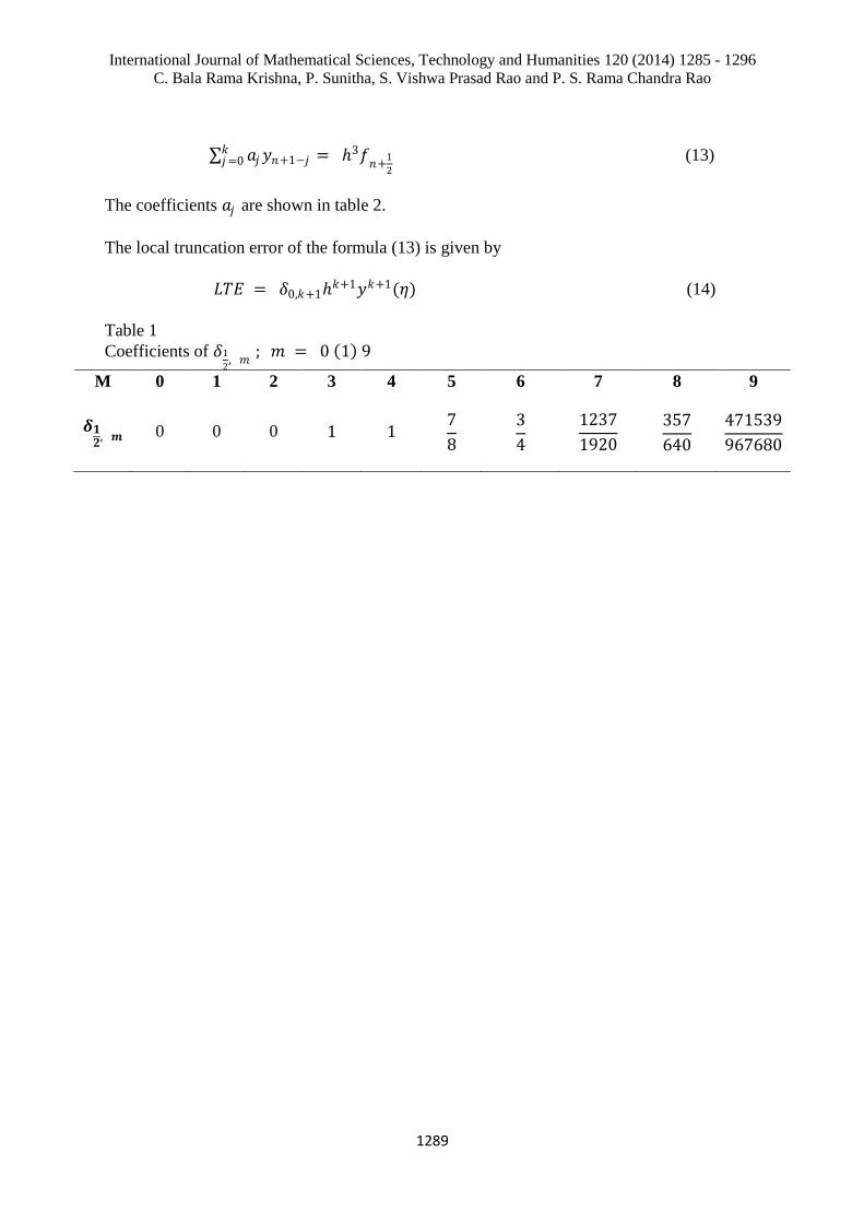
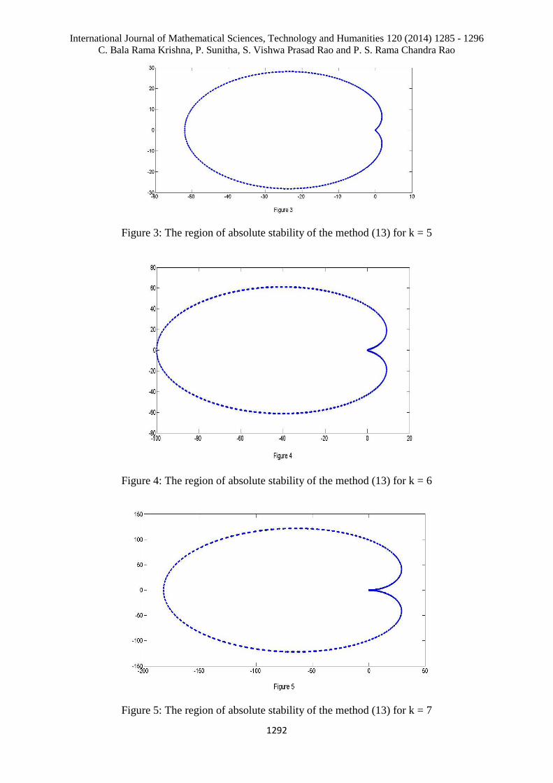
The regions of absolute stability of the method for k = 3 (1) 8 are shown in figures 1 to 7 (Taking

real part on x-axis and imaginary part on y-axis). The region of absolute stability is the region lying

outside the boundary.

Figure 1: The region of absolute stability of the method (13) for k = 3




1292






1293



5. Numerical example

In this section, we have considered the differential equation:

𝑦′′′ = 2𝑒𝑥 − 𝑦 , 𝑦 0 = 0, 𝑦′ 0 = 2, 𝑦′′ 0 = 0 (16)

in the interval [0, 2] with h = 0.01 and h = 0.02.

The exact solution of the above problem is 𝑦 = 𝑒𝑥 −𝑒−𝑥

We have applied the ND methods to solve the differential equation and the results are shown in

tables 3 and 4.



1294

(1) The third order numerical differentiation method (13) derived in this paper with k = 4 is

𝑦𝑛+1 = 7

2𝑦𝑛 −

9

2𝑦𝑛−1 +

5

2𝑦𝑛−2 −

1

2𝑦𝑛−3 +

1

2ℎ3𝑓

𝑛+1

2

(17)

(2) The fourth order numerical differentiation method (13) derived in this paper with k = 5 is

𝑦𝑛+1 =91

23𝑦𝑛 −

142

23𝑦𝑛−1 +

110

23𝑦𝑛−2 −

43

23𝑦𝑛−3 +

7

23𝑦𝑛−4 +

8

23ℎ3𝑓

𝑛+1

2

(18)

(3) The fifth order numerical differentiation method (13) derived in this paper with k = 6 is

𝑦𝑛+1 =127

23𝑦𝑛 −

232

29𝑦𝑛−1 +

230

29𝑦𝑛−2 −

133

29𝑦𝑛−3 +

43

29𝑦𝑛−4 −

6

29𝑦𝑛−5 +

8

29ℎ3𝑓

𝑛+1

2

(19)

Table 3

Solution by the fourth order numerical differentiation (ND) method with k = 5 and h = 0.01

X Exact Solution Numerical Solution by

fourth order ND Absolute Error

0 0.0000000000E+00 -1.0939058455E-14 1.0939058455E-14

0.1 2.0033350004E-01 2.0033350004E-01 4.0550895974E-14

0.2 4.0267200508E-01 4.0267200508E-01 9.2925667161E-14

0.3 6.0904058689E-01 6.0904058689E-01 1.4677148386E-13

0.4 8.2150465161E-01 8.2150465161E-01 2.0350388041E-13

0.5 1.0421906110E+00 1.0421906110E+00 2.5734969711E-13

0.6 1.2733071643E+00 1.2733071643E+00 3.1841196346E-13

0.7 1.5171674037E+00 1.5171674037E+00 3.7925218521E-13

0.8 1.7762119644E+00 1.7762119644E+00 4.4919623576E-13

0.9 2.0530334514E+00 2.0530334514E+00 5.1869619710E-13

1 2.3504023873E+00 2.3504023873E+00 5.9641180883E-13

1.1 2.6712949402E+00 2.6712949402E+00 6.7901240186E-13

1.2 3.0189227108E+00 3.0189227108E+00 7.6383344094E-13

1.3 3.3967648746E+00 3.3967648746E+00 8.6020079948E-13

1.4 3.8086030029E+00 3.8086030029E+00 9.7077901273E-13

1.5 4.2585589102E+00 4.2585589102E+00 1.0800249584E-12

1.6 4.7511359064E+00 4.7511359064E+00 1.2132517213E-12

1.7 5.2912638677E+00 5.2912638677E+00 1.3473666627E-12

1.8 5.8843485762E+00 5.8843485762E+00 1.5010215293E-12

1.9 6.5363258231E+00 6.5363258231E+00 1.6635581801E-12

2 7.2537208157E+00 7.2537208157E+00 1.8456347561E-12



1295

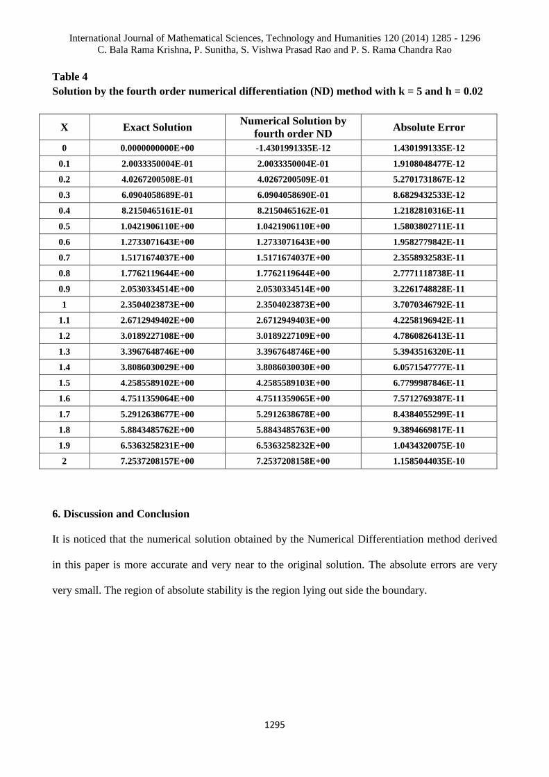
Table 4

Solution by the fourth order numerical differentiation (ND) method with k = 5 and h = 0.02

X Exact Solution Numerical Solution by

fourth order ND Absolute Error

0 0.0000000000E+00 -1.4301991335E-12 1.4301991335E-12

0.1 2.0033350004E-01 2.0033350004E-01 1.9108048477E-12

0.2 4.0267200508E-01 4.0267200509E-01 5.2701731867E-12

0.3 6.0904058689E-01 6.0904058690E-01 8.6829432533E-12

0.4 8.2150465161E-01 8.2150465162E-01 1.2182810316E-11

0.5 1.0421906110E+00 1.0421906110E+00 1.5803802711E-11

0.6 1.2733071643E+00 1.2733071643E+00 1.9582779842E-11

0.7 1.5171674037E+00 1.5171674037E+00 2.3558932583E-11

0.8 1.7762119644E+00 1.7762119644E+00 2.7771118738E-11

0.9 2.0530334514E+00 2.0530334514E+00 3.2261748828E-11

1 2.3504023873E+00 2.3504023873E+00 3.7070346792E-11

1.1 2.6712949402E+00 2.6712949403E+00 4.2258196942E-11

1.2 3.0189227108E+00 3.0189227109E+00 4.7860826413E-11

1.3 3.3967648746E+00 3.3967648746E+00 5.3943516320E-11

1.4 3.8086030029E+00 3.8086030030E+00 6.0571547777E-11

1.5 4.2585589102E+00 4.2585589103E+00 6.7799987846E-11

1.6 4.7511359064E+00 4.7511359065E+00 7.5712769387E-11

1.7 5.2912638677E+00 5.2912638678E+00 8.4384055299E-11

1.8 5.8843485762E+00 5.8843485763E+00 9.3894669817E-11

1.9 6.5363258231E+00 6.5363258232E+00 1.0434320075E-10

2 7.2537208157E+00 7.2537208158E+00 1.1585044035E-10

6. Discussion and Conclusion

It is noticed that the numerical solution obtained by the Numerical Differentiation method derived

in this paper is more accurate and very near to the original solution. The absolute errors are very

very small. The region of absolute stability is the region lying out side the boundary.



1296

References

[1] C. Bala Rama Krishna, P. S. Rama Chandra Rao, S. Vishwa Prasad Rao and B. Nageswara Rao,

Finite Difference Methods for the Solution of a Class of Singular Perturbation Problems,

International Journal of Mathematical Sciences and Engineering Applications, Vol. 7, No. II

(March, 2013), pp. 411 – 421

[2] C. Bala Rama Krishna, P. S. Rama Chandra Rao and D. Srikanth, Special Multi Step Method for the

Solution of a Class of Non Linear Boundary Value Problem, International Journal of Mathematical

Sciences and Engineering Applications, Vol. 8, No. III (May, 2014), pp. 237 – 249

[3] C. E. Froberg, Introduction to Numerical Analysis, Addison Wesley, 1970.

[4] C.W. Gear, Numerical Initial Value Problems in Ordinary Differential Equations, Prentice Hall, 1971.

[5] W.B. Gragg, H.J. Statter, Generalized multistep predictor–corrector methods, Journal of the ACM 11

(1964) 188–209.

[6] P. Henrici, Discrete Variable Methods in Ordinary Differential Equations, Wiley, 1962.

[7] M.K. Jain, Numerical Solution of Differential Equations, Wiley Eastern Limited, 1984.

[8] J. D. Lambert, Computational Methods in Ordinary Differential Equations, Wiley, 1973.

[9] P. Kalyani, and P. S. Rama Chandra Rao, Solution of Boundary Value Problems by Approaching

Spline Techniques, International Journal of Engineering Mathematics, Hindawi Publishing

Corporation, Volume 2013, Article ID 482050

[10] P. Kalyani, and P. S. Rama Chandra Rao, A Conventional Approach for the solution of the fifth order

boundary value problems using sixth degree spline functions, Applied Mathematics, volume 2013,

issue 4, 583 – 588, Scientific Research.

[11] P. S Rama Chandra Rao, Special multistep methods based on numerical differentiation for solving the

initial value problem, Applied Mathematics and Computation 181, (2006), 500–510

numerical solution and stability analysis …internationalejournals.com/pdfs/ijmtah/ijmtah...

Documents