numerical solution of implicitly constrained …heinken/papers/mheinkenschloss_2008a.pdf ·...
TRANSCRIPT
DEPARTMENT OF COMPUTATIONAL AND APPLIED MATHEMATICSRICE UNIVERSITY
TECHNICAL REPORT TR08-05(REVISED JUNE 26, 2012, AND JAN. 16, 2013)
NUMERICAL SOLUTION OF IMPLICITLY CONSTRAINED OPTIMIZATIONPROBLEMS ∗
MATTHIAS HEINKENSCHLOSS †
Abstract. Many applications require the minimization of a smooth function f : Rnu → R whose evaluationrequires the solution of a system of nonlinear equations. This system represents a numerical simulation that must berun to evaluate f . This system of nonlinear equations is referred to as an implicit constraint.
In principle f can be minimized using the steepest descent method or Newton-type methods for unconstrainedminimization. However, for the practical application of derivative based methods for the minimization of f one hasto deal with many interesting issues that arise out of the presence of the implicit constraints that must be solved toevaluate f . This article studies some of these issues, ranging from sensitivity and adjoint techniques for derivativecomputation to implementation issues in Newton-type methods. A discretized optimal control problem governed bythe unsteady Burgers equation is used to illustrate the ideas.
The material in this article is accessible to anyone with knowledge of Newton-type methods for finite dimen-sional unconstrained optimization. Many of the concepts discussed in this article extend to and are used in areassuch as optimal control and PDE constrained optimization.
Key words. Unconstrained minimization, implicit constraints, adjoints, sensitivities, Newton’s method, nonlin-ear programming, optimal control, Burgers equation.
AMS subject classifications. 49M37, 65K05, 90C53, 90C55
1. Introducton. We are interested in the solution of
minu∈U
f (u), (1.1)
where U is a closed convex subset of Rnu , such as U = Rnu or U = [−1,1]nu , and f : U → Ris a smooth function. The numerical solution of (2.1) using gradient-based and Newton-typemethods is discussed in most courses on Numerical Analysis (at least for the case U = Rnu )and in courses on Optimization. Many textbooks such as [12, 22, 26] provide an excellentintroduction into these methods. We investigate their application in the case where the eval-uation of objective function f requires the solution of a system of nonlinear equations. Thissituation arises in many science and engineering applications in which the evaluation of theobjective function involves a simulation. We refer to the system of nonlinear equations (thesimulation) as an implicit constraint. In theory standard optimization algorithms, such asthose discussed in the textbooks [12, 22, 26] can be applied to the solution of (1.1). However,the practical application of these methods quickly leads to interesting questions related to
• gradient and Hessian computations for objective functions f whose evaluation in-volves the solution of an implicit constraint,
• software design issues arising in the implementation of gradient based methods forthe solution of (1.1),
• development of optimization algorithms for problems with inexact function andderivative information.
∗This research was supported in part by NSF grant DMS-0511624 and AFOSR grant FA9550-06-1-0245†Department of Computational and Applied Mathematics, MS-134, Rice University, 6100 Main Street, Houston,
TX 77005-1892 ([email protected]).
1
2 M. HEINKENSCHLOSS
In this paper we will formulate these questions more carefully and explore answers.As an example for an optimization problem (1.1) in which the evaluation of the objective
function requires the solution of a system of nonlinear equations, consider the design ofan airplane wing. Assume that we want to determine the shape of the wing to optimizethe performance of the aircraft. We measure the performance of the aircraft by the ratioof lift over drag. If we assume that the wing can be represented using a combination ofsurfaces parameterized by u = (u1, . . . ,unu), then we arrive at an optimization problem in u.We want to find the shape of the wing represented by u such that the ratio of lift over dragis maximized. Of course, we can convert the maximization problems into a minimizationproblem by minimizing the negative ratio of lift over drag. However, to compute the ratio oflift over drag for a given wing shape specified by u, we need to solve a complex system ofdifferential equations, the Navier-Stokes equations, to obtain the velocity and pressure of theair flowing around the aircraft. From the velocity and pressure we are then able to computelift and drag. Thus the optimization problem which is of the form (1.1) and which on thesurface looks relatively simple is actually quite complicated because of the simulation, herethe solution of the Navier-Stokes equations, required to evaluate the objective function.
How does the presence of the simulation required for the evaluation of the objective func-tion (1.1) impact the application of gradient based optimization algorithms for the solutionof (1.1)? We will explore answers to this question in a less complicated situation than thatof the wing design problem described before. We assume that the simulation by a systemof nonlinear algebraic equations. This setting allows us to explore the solution of (1.1) us-ing basic results from real analysis, such the implicit function theorem and basic numericaloptimization methods, such as the steepest descent method or Newton’s method. In manyapplications, the simulation is described by a systems of (partial) differential equations. Af-ter discretization of the differential equations, one obtains a system of (nonlinear) algebraicequations and the setting of this paper can be applied. Additionally this setting exposes us tomany concepts that one also counters in, e.g., optimal control problems and optimal designproblems governed by (partial) differential equations.
The Matlab codes used to solve the examples in this paper can be downloaded from
http://www.caam.rice.edu/∼heinken/software
2. Problem Formulation. We are interested in optimization problems (2.1) in whichthe evaluation of f requires the solution of a system of nonlinear equations. More precisely,we assume that
f (u) = f (y(u),u), (2.1)
where y(u) ∈ Rny is the solution of an equation
c(y,u) = 0. (2.2)
Here
f : Rny×nu → R, c : Rny×nu → Rny
are given functions.To distinguish between the implicit function which is defined as the solution of (2.2) and
a vector in Rny , we use the notation y(·) to denote the implicit function and y to denote a vectorin Rny . Furthermore, we use subscripts y and u to denote partial derivatives. For examplecy(y,u)∈Rny×ny is the partial Jacobian of the function c with respect to y and ∇u f (y,u)∈Rnu
is the partial gradient of the function f with respect to u
Numerical Solution of Implicitly Constrained Optimization Problems 3
To make the formulation (1.1), (2.1), (2.2) rigorous, we make the following assumptions.ASSUMPTION 2.1.• For all u ∈U there exists a unique y ∈ Rny such that c(y,u) = 0.• There exists an open set D ⊂ Rny×nu with {(y,u) : u ∈U, c(y,u) = 0} ⊂ D such
that f and c are twice continuously differentiable on D.• The inverse cy(y,u)−1 exists for all (y,u) ∈ {(y,u) : u ∈U, c(y,u) = 0}.
Under these assumptions there exists a twice continuously differentiable function
y : Rnu → Rny
defined by
c(y(u),u) = 0.
Note that our Assumptions 2.1 are stronger than those required in the implicit function the-orem. The standard assumptions of the implicit function theorem, only guarantee the localexistence of the implicit function y(·) and the differentiability of this function.
We call (1.1), (2.1), (2.2) an implicitly constrained optimization problem because thesolution of (2.2) is invisible to the optimization algorithm. Of course, in principle one canformulate (1.1), (2.1), (2.2) as an equality constrained optimization problem. In fact, since yis tied to u via the implicit equation (2.2), we could just include this equation into the problemformulation and reformulate (1.1), (2.1), (2.2) as
min f (y,u),s.t. c(y,u) = 0,
u ∈U.(2.3)
In (2.3), the optimization variables are y ∈ Rny and u ∈ Rnu . The formulation (2.3) can havesignificant advantages over (1.1), (2.1), (2.2), but in many applications the formulation of theoptimization problem as a constrained problem may not be possible, for example, because ofthe huge size of y, which in applications can easily be many millions. We will return to theissue of solving the implicitly constrained problem (1.1), (2.1), (2.2) versus the solving theconstrained problem (2.3) later. First, we focus on the solution of (1.1), (2.1), (2.2).
There are many algorithms for the solution of (1.1). See, e.g., the textbooks [7, 12, 22,26]. We state a simple version of the Newton-Conjugate Gradient method for solving (1.1)with U = Rnu . The Newton equation ∇2 f (uk)sk = −∇ f (uk) is solved approximately usingthe conjugate gradient (CG) method. The CG method is truncated if the Newton systemresidual is sufficiently small, more precisely
‖∇2 f (uk)sk +∇ f (uk)‖2 ≤ ηk‖∇ f (uk)‖2,
ηk ∈ (0,1), or if a direction of negative curvature is detected. Once the direction sk is com-puted, a simple Armijo line-search procedure is used to compute the step-size αk. See, e.g.,[22, 26] for more details.
ALGORITHM 2.2 (Newton-CG Method with Armijo Line-Search).1. Given u0 and gtol > 0. Set k = 0.2. Compute ∇ f (uk).3. If ‖∇ f (uk)‖< gtol stop.4. Compute ∇2 f (uk).5. Apply the CG method to compute an approximate solution of the Newton equation
∇2 f (uk)sk =−∇ f (uk) (we use i as the iteration index in the CG method):
4 M. HEINKENSCHLOSS
5.1. Set ηk ∈ (0,1), sk = 0 and pk,0 = rk,0 =−∇ f (uk).5.2. For i = 0,1,2, . . . do
i. If ‖rk,i‖2 < ηk‖rk0‖2 goto 5.3.ii. Compute qk,i = ∇2 f (uk)pi.
iii. If pTk,iqk,i < 0 goto 5.3.
iv. γk,i = ‖rk,i‖2/pTk,iqk,i.
v. sk = sk + γk,i pk,i .vi. rk,i+1 = rk,i− γk,iqk,i.
vii. βk,i = ‖rk,i+1‖2/‖rk,i‖2 .viii. pk,i+1 = rk,i+1 +βk,i pk,i .
5.3. If i = 0 set sk =−∇ f (uk).6. Perform Armijo line-search.
6.1. Set αk = 1 and evaluate f (uk +αksk).6.2. While f (uk +αksk)> f (uk)+10−4αksT
k ∇ f (uk) doi. Set αk = αk/2 and evaluate f (uk +αksk).
7. Set uk+1 = uk +αksk, k← k+1. Goto 2.Newton-CG Algorithm 2.2 requires the computation of gradients ∇ f (uk) and the appli-
cation of Hessians ∇2 f (uk) to vectors pi. We will discuss how to accomplish these tasks inthe following two sections.
3. Gradient Computations. Under Assumption 2.1, the implicit function theorem guar-antees the differentiability of y(·). The Jacobian of y(·) is the solution of
cy(y,u)|y=y(u)yu(u) =−cu(y,u)|y=y(u). (3.1)
To simplify the notation we write cy(y(u),u) and cu(y(u),u) instead of cy(y,u)|y=y(u) andcu(y,u)|y=y(u), respectively. With this notation, we have
yu(u) =−cy(y(u),u)−1cu(y(u),u). (3.2)
The derivative yu(u) is also called the sensitivity (of y with respect to u).Since y(·) is differentiable, the function f is differentiable and its gradient is given by
∇ f (u) = yu(u)T∇y f (y(u),u)+∇u f (y(u),u) (3.3)
=−cu(y(u),u)T cy(y(u),u)−T∇y f (y(u),u)+∇u f (y(u),u).
Note that if we define the matrix
W (y,u) =(−cy(y,u)−1cu(y,u)
I
), (3.4)
then
W (y(u),u) =(
yu(u)I
)(3.5)
and the gradient of f can be written as
∇ f (u) =W (y(u),u)T∇x f (y(u),u). (3.6)
The matrix W (y,u) will play a role later.Equation (3.3) suggests the following method for computing the gradient.
Numerical Solution of Implicitly Constrained Optimization Problems 5
ALGORITHM 3.1 (Gradient Computation Using Sensitivities).1. Given u, solve c(y,u) = 0 for y (if not done already). Denote the solution by y(u).2. Compute the sensitivities S = yu(u) by solving
cy(y(u),u)S =−cu(y(u),u).3. Compute ∇ f (u) = ST ∇y f (y(u),u)+∇u f (y(u),u).
The computation of the sensitivity matrix S requires the solution of nu systems of lin-ear equations cy(y(u),u)S = −cu(y(u),u), all of which have the same system matrix butdifferent right hand sides. If nu is large this can be expensive. The gradient computationcan be executed more efficiently since for the computation of ∇ f (u) we do not need S,but only the application of ST to ∇y f (y(u),u). If we revisit (3.3), we can define λ(u) =−cy(y(u),u)−T ∇y f (y(u),u), or, equivalently, we can define λ(u) ∈ Rny as the solution of
cy(y(u),u)Tλ =−∇y f (y(u),u). (3.7)
In optimization problems (2.1), (2.2) arising from discretized optimal control problems, thesystem (3.7) are called the (discrete) adjoint equations and λ(u) is the (discrete) adjoint. Withthis quantity, the gradient can now be written as
∇ f (u) = ∇u f (y(u),u)+ cu(y(u),u)Tλ(u), (3.8)
which suggests the so-called adjoint equation method for computing the gradient.ALGORITHM 3.2 (Gradient Computation Using Adjoints).
1. Given u, solve c(y,u) = 0 for y (if not done already).2. Solve the adjoint equation cy(y(u),u)T λ =−∇y f (y(u),u) for λ. Denote the solution
by λ(u).3. Compute ∇ f (u) = ∇u f (y(u),u)+ cu(y(u),u)T λ(u).
The gradient computation using the adjoint equation method can also be expressed usingthe Lagrangian
L(y,u,λ) = f (y,u)+λT c(y,u) (3.9)
corresponding to the constraint problem (2.3). Using the Lagrangian, the equation (3.7) canbe written as
∇yL(y,u,λ)|y=y(u),λ=λ(u) = 0. (3.10)
Moreover, (3.8) can be written as
∇ f (u) = ∇uL(y,u,λ)|y=y(u),λ=λ(u). (3.11)
The adjoint equations (3.7) or (3.10) are easy to write down in this abstract setting, but(hand) generating a code to set up and solve the adjoint equations can be quite a differentmatter. This will become somewhat apparent when we discuss a simple optimal controlexample in Section 6. The following observation can be used to generate some checks thatindicate the correctness of the adjoint code. Assume that we have a code that for given ucomputes the solution y of c(y,u) = 0. Often it is not too difficult to derive from this a codethat for given r computes the solution s of cy(y,u)s = r. If λ solves the adjoint equationcy(y,u)T λ =−∇y f (y,u), then
−sT∇y f (y,u) = sT cy(y,u)T
λ = rTλ (3.12)
must hold.
6 M. HEINKENSCHLOSS
4. Hessian Computations. Since we assume f and c to be twice continuously differen-tiable, the function f is twice continuous differentiable. The Hessian of f can be computedfrom (3.11). In fact, we have already computed the derivative of y(·) in (3.2) using the im-plicit function theorem. Analogously we can apply the implicit function theorem to (3.7) orequivalently (3.10) to compute the derivative of λ(·). Differentiating (3.10) gives
∇yyL(y,u,λ)|y=y(u),λ=λ(u) yu(u)+∇yuL(y,u,λ)|y=y(u),λ=λ(u)
+∇yλL(y,u,λ)|y=y(u),λ=λ(u) λu(u) = 0.
If we use ∇yλL(y,u,λ) = cy(y,u)T and (3.2) in the previous equation we find that
λu(u) = cy(y(u),u)−T [∇yyL(y(u),u,λ(u))cy(y(u),u)−1cu(y(u),u)
−∇yuL(y(u),u,λ(u))]. (4.1)
To simplify the expression, we have used the notation ∇yyL(y(u),u,λ(u)) instead of∇yyL(y,u,λ)|y=y(u),λ=λ(u) yu(u) and analogous notation for the other derivatives of L. Wewill continue to use this notation in the following.
Now we can compute the Hessian of f by differentiating (3.11),
∇2 f (u) = ∇uyL(y(u),u,λ(u))yu(u)+∇uuL(y(u),u,λ(u))
+∇uλL(y(u),u,λ(u))λu(u). (4.2)
If we insert (4.1) and (3.2) into (4.2) and observe that ∇uλL(y(u),u,λ(u)) = cu(y(u),u) theHessian can be written as
∇2 f (u) = cu(y(u),u)T cy(y(u),u)−T
∇yyL(y(u),u,λ(u))cy(y(u),u)−1cu(y(u),u)
−cu(y(u),u)T cy(y(u),u)−T∇yuL(y(u),u,λ(u))
−∇uyL(y(u),u,λ(u))cy(y(u),u)−1cu(y(u),u)+∇uuL(y(u),u,λ(u))
=W (y(u),u)T(
∇yyL(y(u),u,λ(u)) ∇yuL(y(u),u,λ(u))∇uyL(y(u),u,λ(u)) ∇uuL(y(u),u,λ(u))
)W (y(u),u). (4.3)
Obviously the identities (4.3) can be used to compute the Hessian. However, in manycases, the computation of the Hessian is too expensive. In that case optimization algorithms,such as the Newton-CG Algorithm 2.2 , that only require the computation of Hessian–times–vector products ∇2 f (u)v can be used. Using the equality (4.3) Hessian–times–vector productscan be computed as follows.
ALGORITHM 4.1 (Hessian–Times–Vector Computation).1. Given u, solve c(y,u) = 0 for y (if not done already). Denote the solution by y(u).2. Solve the adjoint equation cy(y(u),u)T λ=−∇y f (y(u),u) for λ (if not done already).
Denote the solution by λ(u).3. Solve the equation cy(y(u),u)w = cu(y(u),u)v.4. Solve the equation
cy(y(u),u)T p = ∇yyL(y(u),u,λ(u))w−∇yuL(y(u),u,λ(u))v.5. Compute
∇2 f (u)v = cu(y(u),u)T p−∇uyL(y(u),u,λ(u))w+∇uuL(y(u),u,λ(u))v.Hence, if y(u) and λ(u) are already known, then the computation of ∇2 f (u)v requires
the solution of two linear equations. One similar to the linearized state equation, Step 3, andone similar to the adjoint equation, Step 4.
We conclude this section with an observation concerning the connection between theNewton equation ∇2 f (u)su =−∇ f (u) or the Newton–like equation H su =−∇ f (u) and the
Numerical Solution of Implicitly Constrained Optimization Problems 7
solution of a quadratic program. These observations also emphasize the connection betweenthe implicitly constrained problem (2.1) and the nonlinear programming problem (2.3).
THEOREM 4.2. Let cy(y(u),u) be invertible and let ∇2 f (u) be symmetric positivesemidefinite. The vector su solves the Newton equation
∇2 f (u)su =−∇ f (u) (4.4)
if and only if (sy,su) with sy = cy(y(u),u)−1cu(y(u),u)su solves the quadratic program
min(
∇y f (y,u)∇u f (y,u)
)T ( sysu
)+ 1
2
(sysu
)T (∇yyL(y,u,λ) ∇yuL(y,u,λ)∇uyL(y,u,λ) ∇uuL(y,u,λ)
)(sysu
),
s.t. cy(y,u)sy + cu(y,u)su = 0,(4.5)
where y = y(u) and λ = λ(u).Proof. Every feasible point for (4.5) obeys(
sysu
)=
(cy(y(u),u)−1cu(y(u),u)su
su
)=W (y(u),u)su.
Thus, using (3.6) and (4.3), we see that (4.5) is equivalent to
minsu
sTu ∇ f (u)+ 1
2 sTu ∇
2 f (u)su. (4.6)
The desired result now follows from the equivalence of (4.5) and (4.6).Similarly, one can show the following result.THEOREM 4.3. Let cy(y(u),u) be invertible and let H ∈ Rnu×nu be a symmetric positive
semidefinite matrix. The vector su solves the Newton–like equation
H su =−∇ f (u), (4.7)
if and only if (sy,su) with sy = cy(y(u),u)−1cu(y(u),u)su solves the quadratic program
min(
∇y f (y,u)∇u f (y,u)
)T ( sysu
)+ 1
2
(sysu
)T ( 0 00 H
)(sysu
),
s.t. cy(y,u)sy + cu(y,u)su = 0,
(4.8)
where y = y(u) and λ = λ(u).
5. Gauss-Newton. In this section we assume that f is the form
f (y,u) = 12‖Qy−d‖2
2 +R(u) (5.1)
where Q ∈ Rm×ny is a given matrix, d ∈ Rm is a given vector, and R : Rnu → R is a twicecontinuously differentiable function. This type of objective function arises in data fittingproblems, were Qy are observations of the system state, d are data, and R(u) is a regularizationterm.
The reduced objective function corresponding to (5.1) is
f (u) = 12‖Qy(u)−d‖2
2 +R(u), (5.2)
where y(u) is the unique solution of c(y,u) = 0. The Gauss-Newton method minimizes f bysolving a sequence of quadratic problems
minsu
12‖Qyu(u)su +Qy(u)−d‖2
2 +∇R(u)T su +12 sT
u ∇2R(u)su. (5.3)
8 M. HEINKENSCHLOSS
We have
12‖Qyu(u)su +Qy(u)−d‖2
2 +∇R(u)T su +12 sT
u ∇R(u)su
= 12‖Qy(u)−d‖2
2 +(Qy(u)−d)T Qyu(u)su +12 sT
u yu(u)QT Qyu(u)su
+∇R(u)T su +12 sT
u ∇2R(u)su.
The Gauss-Newton approximation of the Hessian ∇2 f (u) is
G(u) = yu(u)QT Qyu(u)+∇2R(u). (5.4)
Note that G(u) is obtained from ∇2 f (u) in (4.3) by replacing L(y,u,λ) = 12‖Qy− d‖2
2 +
R(u) + λT c(y,u) with L(y(u),u,0) = 12‖Qy− d‖2
2 + R(u). Note that if Qy = d, then theLagrange multiplier λ = −cy(y,u)−1∇y f (y,u) = −cy(y,u)−1QT (Qy− d) = 0, i.e., for zeroresidual problems, the Gauss-Newton Hessian approximation is equal to the Hessian.
If we insert (3.2) into (5.4) the Gauss-Newton approximation of the Hessian can be writ-ten as
∇2 f (u) = cu(y(u),u)T cy(y(u),u)−T QT Qcy(y(u),u)−1cu(y(u),u)+∇
2R(u)
=W (y(u),u)T(
QT Q 00 ∇2R(u)
)W (y(u),u). (5.5)
The Gauss–Newton–Hessian–times–vector products can be computed as follows. (Step2 is left empty to facilitate comparison with Algorithm 4.1, see below.)
ALGORITHM 5.1 (Gauss–Newton–Hessian–Times–Vector Computation).1. Given u, solve c(y,u) = 0 for y (if not done already). Denote the solution by y(u).2. (Nothing needs to be done in this step.)3. Solve the equation cy(y(u),u)w = cu(y(u),u)v.4. Solve the equation cy(y(u),u)T p = QT Qw.5. Compute G(u)v = cu(y(u),u)T p+∇2R(u)v.
Note that ∇yyL(y(u),u,0) = QT Q, ∇yuL(y(u),u,0) = 0, ∇uuL(y(u),u,0) = 0, and∇uuL(y(u),u,0) = ∇2R(u). If we compare Algorithms 4.1 and 5.1, then we see that Gauss–Newton–Hessian–times–vector product is computed by using Algorithm 4.1 with λ(u) = 0.
Analogously to Theorem 4.2 we can show the following result.THEOREM 5.2. Let cy(y(u),u) be invertible. The vector su solves the Gauss-Newton
subproblem
minsu
12‖Qyu(u)su +Qy(u)−d‖2
2 +∇R(u)T su +12 sT
u ∇2R(u)su (5.6)
if and only if (sy,su) with sy = cy(y(u),u)−1cu(y(u),u)su solves the quadratic program
min(
QT (Qy−d)∇R(u)
)T ( sysu
)+ 1
2
(sysu
)T ( QT Q 00 ∇2R(u)
)(sysu
),
s.t. cy(y,u)sy + cu(y,u)su = 0,
(5.7)
where y = y(u).
Numerical Solution of Implicitly Constrained Optimization Problems 9
6. Optimal Control of Burgers’ Equation.
6.1. The Infinite Dimensional Problem. We demonstrate the gradient and Hessiancomputation using an optimal control problems governed by the so-called Burgers’ equation.The Burgers equation can be viewed as the Navier-Stokes equations in one space dimensionand it was introduced by Burgers [9, 10]. We first state the optimal control problem in thedifferential equation setting and then introduce a simple discretization to arrive at a finitedimensional problem of the type (2.1).
We want to minimize
minu
12
∫ T
0
∫ 1
0(y(x, t)− z(x, t))2 +ωu2(x, t)dxdt, (6.1a)
where y is the solution of
∂
∂t y(x, t)−ν∂2
∂x2 y(x, t)+ ∂
∂x y(x, t)y(x, t) = r(x, t)+u(x, t) (x, t) ∈ (0,1)× (0,T ),
y(0, t) = y(1, t) = 0 t ∈ (0,T ),
y(x,0) = y0(x) x ∈ (0,1),(6.1b)
where z : (0,1)× (0,T )→ R, r : (0,1)× (0,T )→ R, and y0 : (0,1)→ R are given functionsand ω,ν > 0 are given parameters. The parameter ν > 0 is also called the viscosity and thedifferential equation (6.1b) is known as the (viscous) Burgers’ equation. The problem (6.1)is studied, e.g., in [25, 31]. As we have mentioned earlier, (6.1) can be viewed as a first steptowards solving optimal control problems governed by the Navier-Stokes equations [2, 17].
In this context of (6.1) the function u is called the control, y is called the state, and(6.1b) is called the state equation. We do not study the infinite dimensional problem (6.1),but instead consider a discretization of (6.1).
6.2. Problem Discretization. To discretize (6.1) in space, we use piecewise linear finiteelements. For this purpose, we multiply the differential equation in (6.1b) by a sufficientlysmooth function ϕ which satisfies ϕ(0) = ϕ(1) = 0. Then we integrate both sides over (0,1),and apply integration by parts. This leads to
ddt
∫ 1
0y(x, t)ϕ(x)dx+ν
∫ 1
0
∂
∂xy(x, t)
ddx
ϕ(x)dx+∫ 1
0
∂
∂xy(x, t)y(x, t)ϕ(x)dx
=∫ 1
0(r(x, t)+u(x, t))ϕ(x)dx. (6.2)
Now we subdivide the spatial interval [0,1] into n subintervals [xi−1,xi], i = 1, . . . ,n, withxi = ih and h = 1/n. We define piecewise linear (‘hat’) functions
ϕi(x) =
h−1(x− (i−1)h) x ∈ [(i−1)h, ih]∩ [0,1],h−1(−x+(i+1)h) x ∈ [ih,(i+1)h]∩ [0,1],0 else
i = 0, . . . ,n, (6.3)
which satisfy ϕ j(x j) = 1 and ϕ j(xi) = 0, i 6= j.We approximate y and u by functions of the form
yh(x, t) =n−1
∑j=1
y j(t)ϕ j(x) (6.4)
10 M. HEINKENSCHLOSS
and
uh(x, t) =n
∑j=0
u j(t)ϕ j(x). (6.5)
We set
~y(t) = (y1(t), . . . ,yn−1(t))T and ~u(t) = (u0(t), . . . ,un(t))T ,
If we insert the approximations (6.4), (6.5) into (6.2) and require (6.2) to hold for for ϕ = ϕi,i = 1, . . . ,n−1, then we obtain the system of ordinary differential equations
Mhddt~y(t)+Ah~y(t)+Nh(~y(t))+Bh~u(t) = rh(t), t ∈ (0,T ), (6.6)
where Mh,Ah ∈ R(n−1)×(n−1), Bh ∈ R(n−1)×(n+1), rh(t) ∈ Rn−1, and Nh(~y(t)) ∈ Rn−1 are ma-trices or vectors with entries
(Mh)i j =∫ 1
0ϕ j(x)ϕi(x)dx,
(Ah)i j = ν
∫ 1
0
ddx
ϕ j(x)ddx
ϕi(x)dx,
(Bh)i j =−∫ 1
0ϕ j(x)ϕi(x)dx,
(Nh(~y(t)))i =n−1
∑j=1
n−1
∑k=1
∫ 1
0
ddx
ϕ j(x)ϕk(x)ϕi(x)dx yk(t)y j(t),
(rh(t))i =∫ 1
0r(x, t)ϕi(x)dx.
If we insert (6.4), (6.5) into (6.1), we obtain∫ T
0
12~y(t)T Mh~y(t)+(gh(t))T~y(t)+
ω
2~u(t)T Qh~u(t)dt +
∫ T
0
∫ 1
0
12
y2(x, t)dxdt,
where Mh ∈ R(n−1)×(n−1) is defined as before and Qh ∈ R(n+1)×(n+1), gh(t) ∈ R(n−1) are amatrix and vector with entries
(Qh)i j =∫ 1
0ϕ j(x)ϕi(x)dx,
(gh(t))i =−∫ 1
0z(x, t)ϕi(x)dx.
Thus a semi–discretization of the optimal control problem (6.1) is given by
min~u
∫ T
0
12~y(t)T Mh~y(t)+(gh(t))T~y(t)+
ω
2~u(t)T Qh~u(t)dt, (6.7a)
where~y(t) is the solution of
Mhddt~y(t)+Ah~y(t)+Nh(~y(t))+Bh~u(t) = rh(t), t ∈ (0,T ),
~y(0) = ~y0,(6.7b)
where~y0 = (y0(h), . . . ,y0(1−h))T .
Numerical Solution of Implicitly Constrained Optimization Problems 11
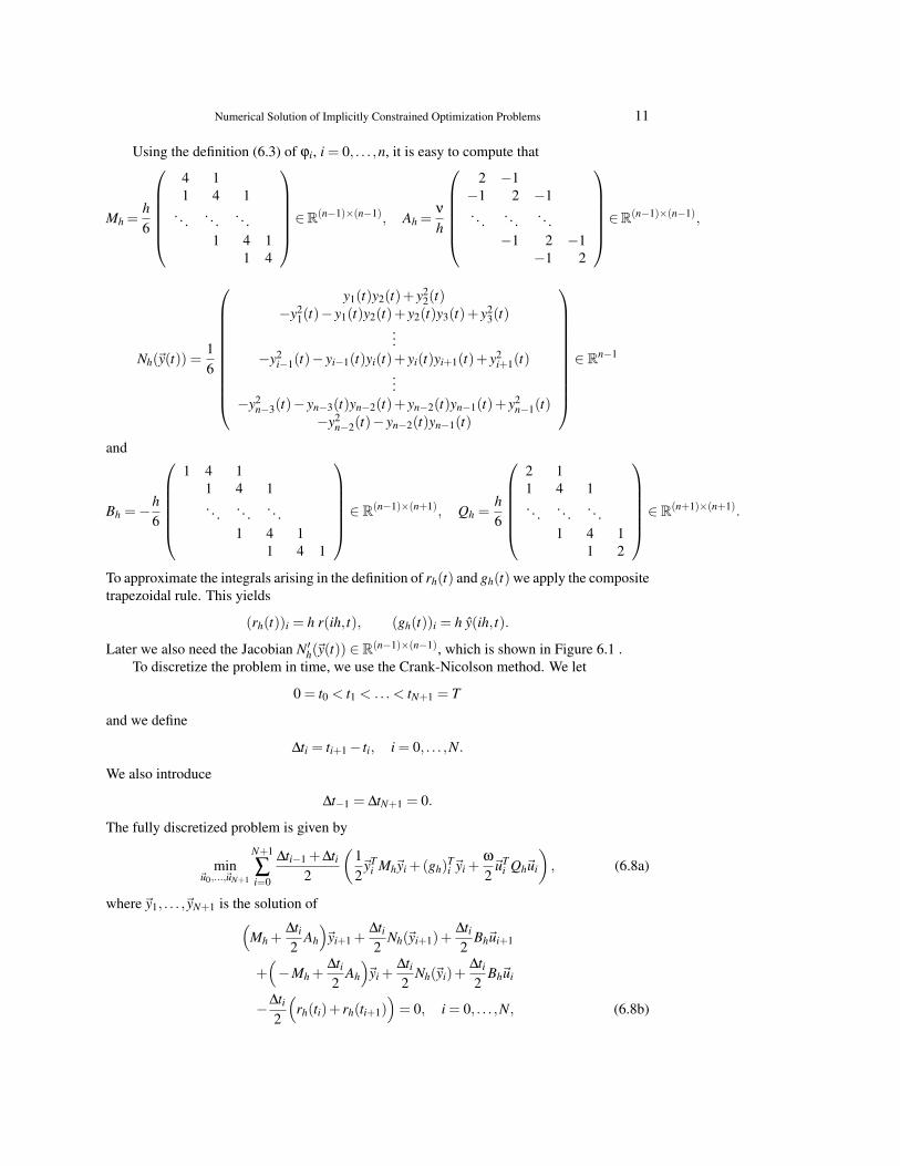
Using the definition (6.3) of ϕi, i = 0, . . . ,n, it is easy to compute that
Mh =h6
4 11 4 1
. . . . . . . . .1 4 1
1 4
∈R(n−1)×(n−1), Ah =ν
h
2 −1−1 2 −1. . . . . . . . .
−1 2 −1−1 2
∈R(n−1)×(n−1),
Nh(~y(t)) =16
y1(t)y2(t)+ y22(t)
−y21(t)− y1(t)y2(t)+ y2(t)y3(t)+ y2
3(t)...
−y2i−1(t)− yi−1(t)yi(t)+ yi(t)yi+1(t)+ y2
i+1(t)...
−y2n−3(t)− yn−3(t)yn−2(t)+ yn−2(t)yn−1(t)+ y2
n−1(t)−y2
n−2(t)− yn−2(t)yn−1(t)
∈ Rn−1
and
Bh =−h6
1 4 1
1 4 1. . . . . . . . .
1 4 11 4 1
∈ R(n−1)×(n+1), Qh =h6
2 11 4 1. . . . . . . . .
1 4 11 2
∈ R(n+1)×(n+1).
To approximate the integrals arising in the definition of rh(t) and gh(t) we apply the compositetrapezoidal rule. This yields
(rh(t))i = h r(ih, t), (gh(t))i = h y(ih, t).
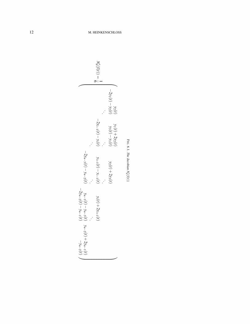
Later we also need the Jacobian N′h(~y(t)) ∈ R(n−1)×(n−1), which is shown in Figure 6.1 .To discretize the problem in time, we use the Crank-Nicolson method. We let
0 = t0 < t1 < .. . < tN+1 = T
and we define
∆ti = ti+1− ti, i = 0, . . . ,N.
We also introduce
∆t−1 = ∆tN+1 = 0.
The fully discretized problem is given by
min~u0,...,~uN+1
N+1
∑i=0
∆ti−1 +∆ti2
(12~yT
i Mh~yi +(gh)Ti ~yi +
ω
2~uT
i Qh~ui
), (6.8a)
where~y1, . . . ,~yN+1 is the solution of(Mh +
∆ti2
Ah
)~yi+1 +
∆ti2
Nh(~yi+1)+∆ti2
Bh~ui+1
+(−Mh +
∆ti2
Ah
)~yi +
∆ti2
Nh(~yi)+∆ti2
Bh~ui
−∆ti2
(rh(ti)+ rh(ti+1)
)= 0, i = 0, . . . ,N, (6.8b)
12 M. HEINKENSCHLOSS
FIG
.6.1.TheJacobian
N′h (~y(t))
N′h (~y(t))
=16
y2 (t)y1 (t)
+2y2 (t)
−2y1 (t)−
y2 (t)y3 (t)−
y1 (t)y2 (t)
+2y3 (t)
......
...−
2yi−
1 (t)−y
i (t)y
i+1 (t)−
yi−
1 (t)y
i (t)+
2yi+
1 (t)...
......
−2y
n−3 (t)−
yn−
2 (t)y
n−1 (t)−
yn−
3 (t)y
n−2 (t)
+2y
n−1 (t)
−2y
n−2 (t)−
yn−
1 (t)−
yn−
2 (t)
Numerical Solution of Implicitly Constrained Optimization Problems 13
and~y0 is given. We denote the objective function in (6.8a) by f and we set
u = (~uT0 , . . . ,~u
TN+1)
T .
We call u the control, y = (~yT1 , . . . ,~y
TN+1)
T the state, and (6.8b) is called the (discretized)state equation.
Like with many applications, the verification that (6.8) satisfies the Assumptions 2.1, es-pecially the first and third one, is difficult. If the set U of admissible controls u is constrainedin a suitable manner and if the parameters ν, h, ∆ti are chosen properly, then it is possible toverify Assumptions 2.1. We ignore this issue and continue as if Assumptions 2.1 are valid for(6.8). In our numerical experiments indicate that this is fine for our problem setting. We alsonote that our simple Galerkin finite element method in space produces only meaningful re-sults if the mesh size h is sufficiently small (relative to the viscosity ν and size of the solutiony). Otherwise the computed solution exhibits spurious oscillations. Again, for our parametersettings, our discretization is sufficient.
Since the Burgers’ equation (6.8b) is quadratic in ~yi+1, the computation of ~yi+1, i =0, . . . ,N, requires the solution of system of nonlinear equations. We apply Newton’s methodto compute the solution~yi+1 of (6.8b). We use the computed state~yi at the previous time stepas the initial iterate in Newton’s method.
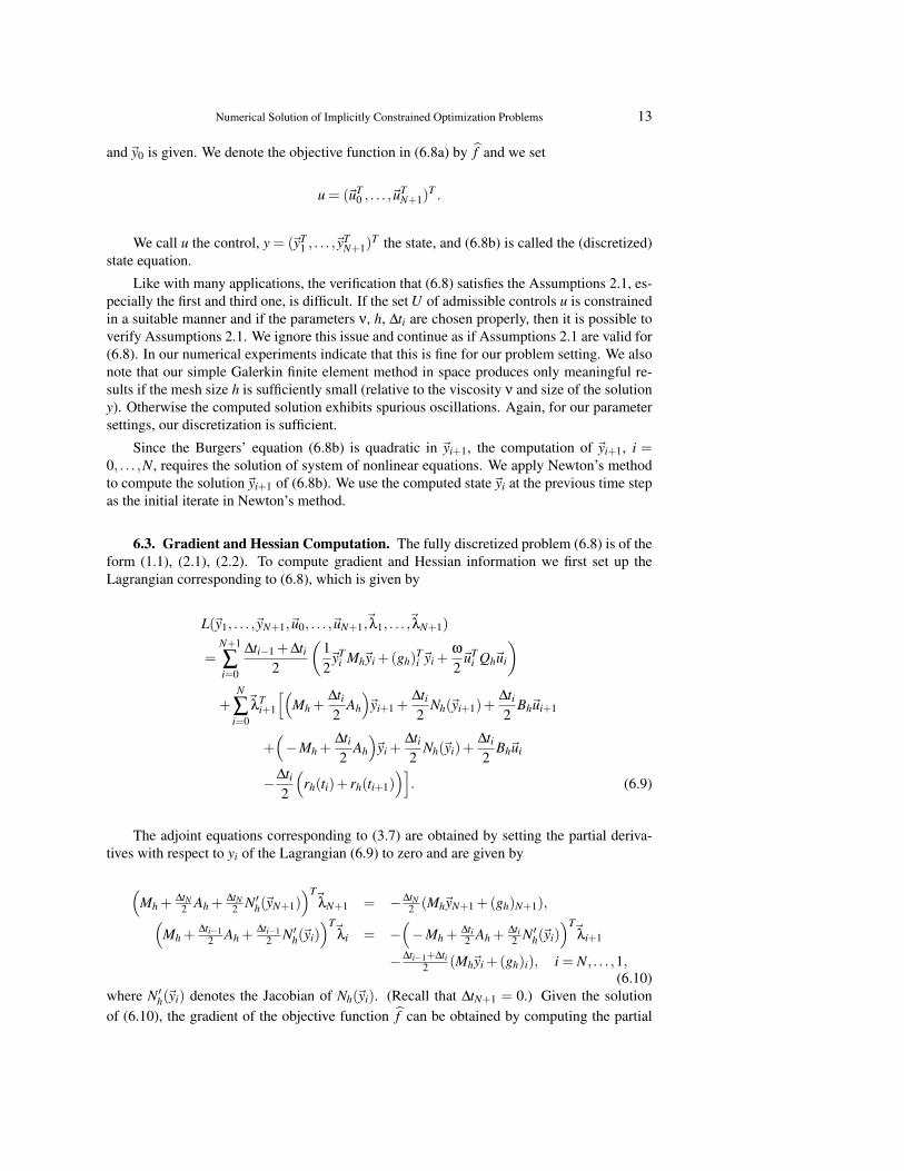
6.3. Gradient and Hessian Computation. The fully discretized problem (6.8) is of theform (1.1), (2.1), (2.2). To compute gradient and Hessian information we first set up theLagrangian corresponding to (6.8), which is given by
L(~y1, . . . ,~yN+1,~u0, . . . ,~uN+1,~λ1, . . . ,~λN+1)
=N+1
∑i=0
∆ti−1 +∆ti2
(12~yT
i Mh~yi +(gh)Ti ~yi +
ω
2~uT
i Qh~ui
)+
N
∑i=0
~λTi+1
[(Mh +
∆ti2
Ah
)~yi+1 +
∆ti2
Nh(~yi+1)+∆ti2
Bh~ui+1
+(−Mh +
∆ti2
Ah
)~yi +
∆ti2
Nh(~yi)+∆ti2
Bh~ui
−∆ti2
(rh(ti)+ rh(ti+1)
)]. (6.9)
The adjoint equations corresponding to (3.7) are obtained by setting the partial deriva-tives with respect to yi of the Lagrangian (6.9) to zero and are given by
(Mh +
∆tN2 Ah +
∆tN2 N′h(~yN+1)
)T~λN+1 = −∆tN
2 (Mh~yN+1 +(gh)N+1),(Mh +
∆ti−12 Ah +
∆ti−12 N′h(~yi)
)T~λi = −
(−Mh +
∆ti2 Ah +
∆ti2 N′h(~yi)
)T~λi+1
−∆ti−1+∆ti2 (Mh~yi +(gh)i), i = N, . . . ,1,
(6.10)where N′h(~yi) denotes the Jacobian of Nh(~yi). (Recall that ∆tN+1 = 0.) Given the solutionof (6.10), the gradient of the objective function f can be obtained by computing the partial
14 M. HEINKENSCHLOSS
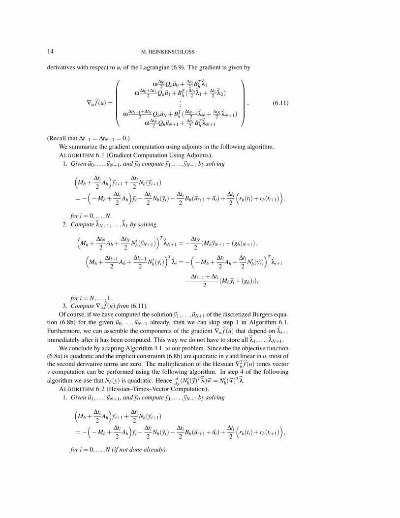
derivatives with respect to ui of the Lagrangian (6.9). The gradient is given by
∇u f (u) =
ω
∆t02 Qh~u0 +
∆t02 BT
h~λ1
ω∆t0+∆t1
2 Qh~u1 +BTh (
∆t02~λ1 +
∆t12~λ2)
...ω
∆tN−1+∆tN2 Qh~uN +BT
h (∆tN−1
2~λN + ∆tN
2~λN+1)
ω∆tN
2 Qh~uN+1 +∆tN
2 BTh~λN+1
. (6.11)
(Recall that ∆t−1 = ∆tN+1 = 0.)We summarize the gradient computation using adjoints in the following algorithm.ALGORITHM 6.1 (Gradient Computation Using Adjoints).
1. Given~u0, . . . ,~uN+1, and~y0 compute~y1, . . . ,~yN+1 by solving(Mh +
∆ti2
Ah
)~yi+1 +
∆ti2
Nh(~yi+1)
=−(−Mh +
∆ti2
Ah
)~yi−
∆ti2
Nh(~yi)−∆ti2
Bh(~ui+1 +~ui)+∆ti2
(rh(ti)+ rh(ti+1)
),
for i = 0, . . . ,N.2. Compute~λN+1, . . . ,~λ1 by solving(
Mh +∆tN2
Ah +∆tN2
N′h(~yN+1))T~λN+1 =−
∆tN2
(Mh~yN+1 +(gh)N+1),(Mh +
∆ti−1
2Ah +
∆ti−1
2N′h(~yi)
)T~λi =−
(−Mh +
∆ti2
Ah +∆ti2
N′h(~yi))T~λi+1
−∆ti−1 +∆ti2
(Mh~yi +(gh)i),
for i = N, . . . ,1.3. Compute ∇u f (u) from (6.11).
Of course, if we have computed the solution~y1, . . . ,~uN+1 of the discretized Burgers equa-tion (6.8b) for the given ~u0, . . . ,~uN+1 already, then we can skip step 1 in Algorithm 6.1.Furthermore, we can assemble the components of the gradient ∇u f (u) that depend on~λi+1
immediately after it has been computed. This way we do not have to store all~λ1, . . . ,~λN+1.We conclude by adapting Algorithm 4.1 to our problem. Since the the objective function
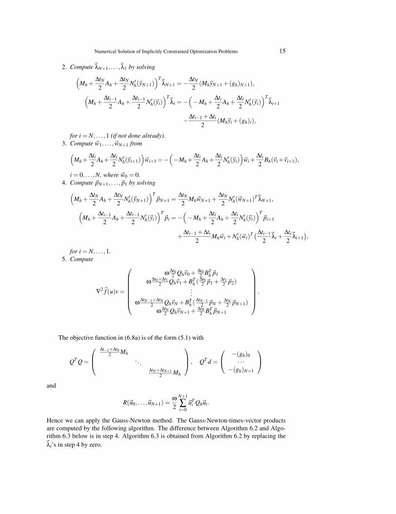
(6.8a) is quadratic and the implicit constraints (6.8b) are quadratic in y and linear in u, most ofthe second derivative terms are zero. The multiplication of the Hessian ∇2
u f (u) times vectorv computation can be performed using the following algorithm. In step 4 of the followingalgorithm we use that Nh(y) is quadratic. Hence d
dy (N′h(~y)
T~λ)~w = N′h(~w)T~λ.
ALGORITHM 6.2 (Hessian–Times–Vector Computation).1. Given~u1, . . . ,~uN+1, and~y0 compute~y1, . . . ,~yN+1 by solving(
Mh +∆ti2
Ah
)~yi+1 +
∆ti2
Nh(~yi+1)
=−(−Mh +
∆ti2
Ah
)~yi−
∆ti2
Nh(~yi)−∆ti2
Bh(~ui+1 +~ui)+∆ti2
(rh(ti)+ rh(ti+1)
),
for i = 0, . . . ,N (if not done already).
Numerical Solution of Implicitly Constrained Optimization Problems 15
2. Compute~λN+1, . . . ,~λ1 by solving(Mh +
∆tN2
Ah +∆tN2
N′h(~yN+1))T~λN+1 =−
∆tN2
(Mh~yN+1 +(gh)N+1),(Mh +
∆ti−1
2Ah +
∆ti−1
2N′h(~yi)
)T~λi =−
(−Mh +
∆ti2
Ah +∆ti2
N′h(~yi))T~λi+1
−∆ti−1 +∆ti2
(Mh~yi +(gh)i),
for i = N, . . . ,1 (if not done already).3. Compute ~w1, . . . ,~wN+1 from(
Mh+∆ti2
Ah+∆ti2
N′h(~yi+1))~wi+1 =−
(−Mh+
∆ti2
Ah+∆ti2
N′h(~yi))~wi+
∆ti2
Bh(~vi+~vi+1),
i = 0, . . . ,N, where ~w0 = 0.4. Compute ~pN+1, . . . ,~p1 by solving(
Mh +∆tN2
Ah +∆tN2
N′h(~yN+1))T
~pN+1 =∆tN2
Mh~wN+1 +∆tN2
N′h(~wN+1)T~λN+1,(
Mh +∆ti−1
2Ah +
∆ti−1
2N′h(~yi)
)T~pi =−
(−Mh +
∆ti2
Ah +∆ti2
N′h(~yi))T
~pi+1
+∆ti−1 +∆ti
2Mh~wi +N′h(~wi)
T (∆ti−1
2~λi +
∆ti2~λi+1
),
for i = N, . . . ,1.5. Compute
∇2 f (u)v =
ω
∆t02 Qh~v0 +
∆t02 BT
h~p1
ω∆t0+∆t1
2 Qh~v1 +BTh (
∆t02 ~p1 +
∆t12 ~p2)
...ω
∆tN−1+∆tN2 Qh~vN +BT
h (∆tN−1
2 ~pN + ∆tN2 ~pN+1)
ω∆tN
2 Qh~vN+1 +∆tN
2 BTh~pN+1
.
The objective function in (6.8a) is of the form (5.1) with
QT Q =
∆t−1+∆t0
2 Mh. . .
∆tN+∆tN+12 Mh
, QT d =
−(gh)0· · ·
−(gh)N+1
and
R(~u0, . . . ,~uN+1) =ω
2
N+1
∑i=0
~uTi Qh~ui.
Hence we can apply the Gauss-Newton method. The Gauss-Newton-times-vector productsare computed by the following algorithm. The difference between Algorithm 6.2 and Algo-rithm 6.3 below is in step 4. Algorithm 6.3 is obtained from Algorithm 6.2 by replacing the~λi’s in step 4 by zero.
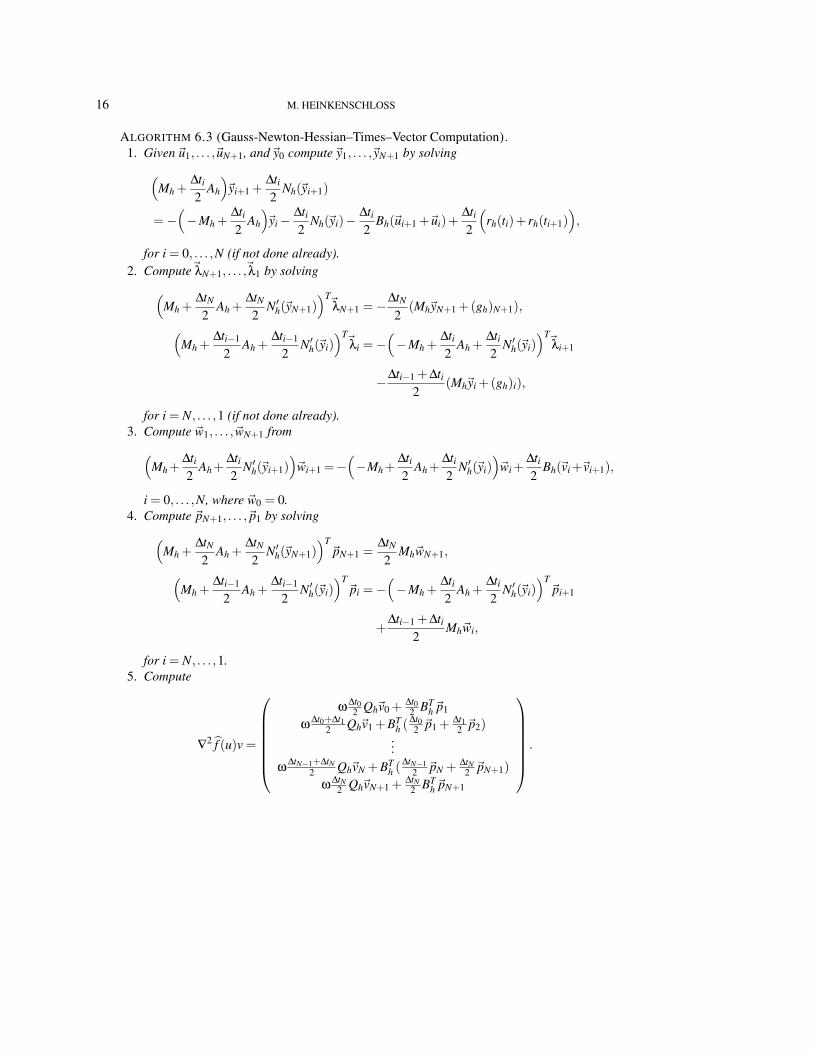
16 M. HEINKENSCHLOSS
ALGORITHM 6.3 (Gauss-Newton-Hessian–Times–Vector Computation).1. Given~u1, . . . ,~uN+1, and~y0 compute~y1, . . . ,~yN+1 by solving(
Mh +∆ti2
Ah
)~yi+1 +
∆ti2
Nh(~yi+1)
=−(−Mh +
∆ti2
Ah
)~yi−
∆ti2
Nh(~yi)−∆ti2
Bh(~ui+1 +~ui)+∆ti2
(rh(ti)+ rh(ti+1)
),
for i = 0, . . . ,N (if not done already).2. Compute~λN+1, . . . ,~λ1 by solving(
Mh +∆tN2
Ah +∆tN2
N′h(~yN+1))T~λN+1 =−
∆tN2
(Mh~yN+1 +(gh)N+1),(Mh +
∆ti−1
2Ah +
∆ti−1
2N′h(~yi)
)T~λi =−
(−Mh +
∆ti2
Ah +∆ti2
N′h(~yi))T~λi+1
−∆ti−1 +∆ti2
(Mh~yi +(gh)i),
for i = N, . . . ,1 (if not done already).3. Compute ~w1, . . . ,~wN+1 from(
Mh+∆ti2
Ah+∆ti2
N′h(~yi+1))~wi+1 =−
(−Mh+
∆ti2
Ah+∆ti2
N′h(~yi))~wi+
∆ti2
Bh(~vi+~vi+1),
i = 0, . . . ,N, where ~w0 = 0.4. Compute ~pN+1, . . . ,~p1 by solving(
Mh +∆tN2
Ah +∆tN2
N′h(~yN+1))T
~pN+1 =∆tN2
Mh~wN+1,(Mh +
∆ti−1
2Ah +
∆ti−1
2N′h(~yi)
)T~pi =−
(−Mh +
∆ti2
Ah +∆ti2
N′h(~yi))T
~pi+1
+∆ti−1 +∆ti
2Mh~wi,
for i = N, . . . ,1.5. Compute
∇2 f (u)v =
ω
∆t02 Qh~v0 +
∆t02 BT
h~p1
ω∆t0+∆t1
2 Qh~v1 +BTh (
∆t02 ~p1 +
∆t12 ~p2)
...ω
∆tN−1+∆tN2 Qh~vN +BT
h (∆tN−1
2 ~pN + ∆tN2 ~pN+1)
ω∆tN
2 Qh~vN+1 +∆tN
2 BTh~pN+1
.
Numerical Solution of Implicitly Constrained Optimization Problems 17
6.4. A Numerical Example. We consider the optimal control problem (6.8) with dataT = 1, ω = 0.05, ν = 0.01, r = 0,
y0(x) ={
1 x ∈ (0, 12 ],
0 else,
and z(x, t) = y0(x), t ∈ (0,T ) (cf. [23]). For the discretization we use nx = 80 spatial subin-tervals and 80 time steps, i.e., ∆t = 1/80.
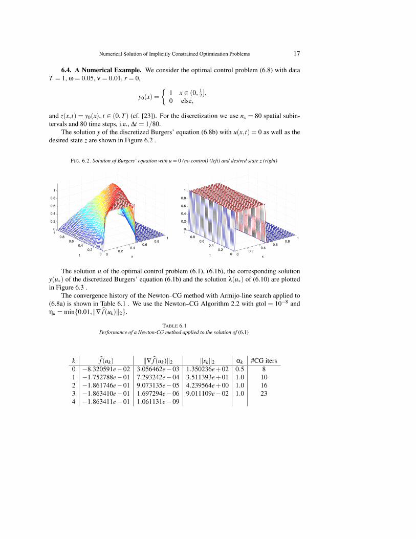
The solution y of the discretized Burgers’ equation (6.8b) with u(x, t) = 0 as well as thedesired state z are shown in Figure 6.2 .
FIG. 6.2. Solution of Burgers’ equation with u = 0 (no control) (left) and desired state z (right)
00.2
0.40.6
0.81
00.2
0.40.6
0.810
0.2
0.4
0.6
0.8
1
xt 00.2
0.40.6
0.81
00.2
0.40.6
0.810
0.2
0.4
0.6
0.8
1
xt
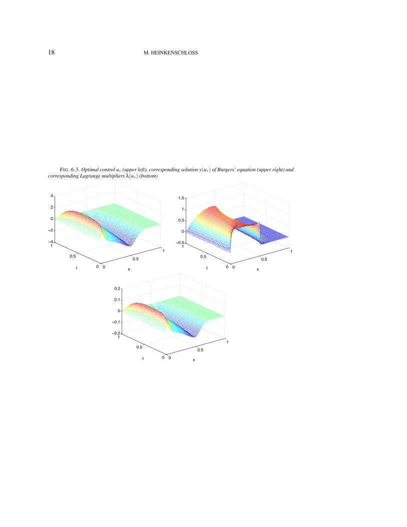
The solution u of the optimal control problem (6.1), (6.1b), the corresponding solutiony(u∗) of the discretized Burgers’ equation (6.1b) and the solution λ(u∗) of (6.10) are plottedin Figure 6.3 .
The convergence history of the Newton–CG method with Armijo-line search applied to(6.8a) is shown in Table 6.1 . We use the Newton–CG Algorithm 2.2 with gtol = 10−8 andηk = min{0.01,‖∇ f (uk)‖2}.
TABLE 6.1Performance of a Newton-CG method applied to the solution of (6.1)
k f (uk) ‖∇ f (uk)‖2 ‖sk‖2 αk #CG iters0 −8.320591e−02 3.056462e−03 1.350236e+02 0.5 81 −1.752788e−01 7.293242e−04 3.511393e+01 1.0 102 −1.861746e−01 9.073135e−05 4.239564e+00 1.0 163 −1.863410e−01 1.697294e−06 9.011109e−02 1.0 234 −1.863411e−01 1.061131e−09
18 M. HEINKENSCHLOSS
FIG. 6.3. Optimal control u∗ (upper left), corresponding solution y(u∗) of Burgers’ equation (upper right) andcorresponding Lagrange multipliers λ(u∗) (bottom)
0
0.5
1
0
0.5
1−4
−2
0
2
4
xt 0
0.5
1
0
0.5
1−0.5
0
0.5
1
1.5
xt
0
0.5
1
0
0.5
1−0.2
−0.1
0
0.1
0.2
xt
Numerical Solution of Implicitly Constrained Optimization Problems 19
6.5. Checkpointing. In Algorithm 6.1 we note that the state equation is solved forwardfor the ~yi’s while the adjoint equation is solved backward for the~λi’s. Moreover the states~yN+1, . . . ,~y1 are needed for the computation of the adjoints~λN+1, . . . ,~λ1. If the size of thestate vectors ~yi is small enough so that all states ~y1, . . . ,~yN+1 can be held in the computermemory, this dependence does not pose a difficulty. However, for many problems, such asflow control problems governed by the unsteady Navier-Stokes equations, the states are toolarge to hold the entire state history in computer memory. In this case one needs to applyso-called checkpointing techniques.
With checkpointing one trades memory for state re-compuations. In a simple schemeone keeps not every state~y0,~y1, . . . ,~yN+1, but only every Mth state~y0,~yM, . . . ,~yN+1 (here weassume that N +1 is an integer multiple of M). In the computation of the adjoint variables~λifor i ∈ {kM+1, . . . ,(k+1)M−1} and some k ∈ {0, . . . ,(N+1)/M} one needs~yi, which hasnot been stored. Therefore, one uses the stored~ykM to re-compute~ykM+1, . . . ,~y(k+1)M−1.
ALGORITHM 6.4 (Gradient Computation Using Adjoints and Simple Checkpointing).Let N and M be such that N +1 is an integer multiple of M.
1. Given~u0, . . . ,~uN+1, and~y0. Store~y0.1.1. For k = 0, . . . ,(N +1)/M−1 solve(
Mh +∆ti2
Ah
)~yi+1 +
∆ti2
Nh(~yi+1)
=−(−Mh +
∆ti2
Ah
)~yi−
∆ti2
Nh(~yi)−∆ti2
Bh(~ui+1 +~ui)+∆ti2
(rh(ti)+ rh(ti+1)
),
for i = kM, . . . ,(k+1)M−1.1.2. Store~y(k+1)M .
2. Adjoint computation.2.1. Compute~λN+1 by solving(
Mh +∆tN2
Ah +∆tN2
N′h(~yN+1))T~λN+1 =−
∆tN2
(Mh~yN+1 +(gh)N+1).
Add the~λN+1 contribution to the appropriate entries of ∇u f (u).2.2. For k = (N +1)/M−1, . . . ,0
2.2.1 Re-compute~ykM+1, . . . ,~y(k+1)M−1 from the stored~ykM by solving(Mh +
∆ti2
Ah
)~yi+1 +
∆ti2
Nh(~yi+1)
=−(−Mh +
∆ti2
Ah
)~yi−
∆ti2
Nh(~yi)−∆ti2
Bh(~ui+1 +~ui)+∆ti2
(rh(ti)+ rh(ti+1)
),
for i = kM, . . . ,(k+1)M−1.2.2.2 Compute~λ(k+1)M−1, . . .
~λkM by solving(Mh +
∆ti−1
2Ah +
∆ti−1
2N′h(~yi)
)T~λi =−
(−Mh +
∆ti2
Ah +∆ti2
N′h(~yi))T~λi+1
−∆ti−1 +∆ti2
(Mh~yi +(gh)i),
for i = (k+1)M−1, . . . ,kM.After ~λi has been computed add the ~λi contribution to the appropriateentries of ∇u f (u).
20 M. HEINKENSCHLOSS
Note that for k = (N + 1)/M − 1 one really does not need to recompute the states~yN+2−M, . . . ,~yN in step 2.2.1, since they are the last states computed in step 1.1. and should bestored there. Algorithm 6.4 requires storage for (N + 1)/M + 1 vectors ~y0,~yM, . . . ,~yN+1, forM−1 vectors~ykM+1, . . . ,~y(k+1)M−1 computed in step 2.2.1, and for one vector~λi. This sim-ple checkpointing scheme has been used in [6] for the solution of an optimal control problemgoverned by the unsteady Navier-Stokes equation.
The simple checkpointing scheme used in Algorithm 6.4 is not optimal in the sense thatgiven a certain memory size to store state information it uses too many state re-computations.The issue of optimal checkpointing is studied in the context of Automatic Differentiation (seealso Section 8). The so-called reverse mode automatic differentiation is closely related togradient computations via the adjoint method. We refer to [15, Sec. 4] for more details. Thepapers [16, 13] discuss implementations of checkpointing schemes and the paper [20] dis-cusses the use of checkpointing schemes for adjoint based gradient computations in optimalcontrol problem governed by the unsteady Navier-Stokes equation.
7. Optimization. In the previous sections we have discussed the computation of gradi-ent and Hessian information for the implicitly constrained optimization problem (1.1), (2.1),(2.2). Thus it seems we should be able to apply a gradient based optimization algorithm, likethe Newton–CG Algorithm 2.2 to solve the problem. In fact, in the previous section we haveused the Newton–CG Algorithm 2.2 to solve the discretized optimal control problem (6.8).However, there are important issues left to be dealt with. These are perhaps not so obviouswhen one deals with the algorithms in the previous sections ‘on paper’, but they becomeapparent when one actually as to implement the algorithms.
7.1. Implicit Constraints.
7.1.1. Avoiding Recomputations of y and λ. If we look at the Newton–CG Algorithm2.2 we see that in each iteration k we have to compute a gradient ∇ f (uk), we have to applythe Hessian ∇2 f (uk) to a number of vectors, and we have to evaluate the function f at sometrial points. In a Matlab implementation of Newton–CG Algorithm 2.2 one may require theuser to supply three functions
function [f] = fval(u, usr_par)function [g] = grad(u, usr_par)function [Hv] = Hessvec(v, u, usr_par)
that evaluate the objective function f (u), evaluate the gradient ∇ f (u), and evaluate theHessian-times-vector product ∇2 f (u)v, respectively. The last argument usr_par is includedto allow he user to pass problem specific parameters to the functions.
Now, if we look at Algorithms 3.1, 3.2, and 4.1 we see that the computation of ∇ f (u)and ∇2 f (u)v all require the computation of y(u). Furthermore, the computation of ∇2 f (u)vrequires the computation of λ(u). Since the computation y(u) can be expensive, we wantto reuse an already computed y(u) rather than to recompute y(u) every time fval, grad, orHessvec is called. Similarly we want to reuse λ(u) which has to be computed as part of thegradient computation in Algorithm 3.2 during subsequent calls of Hessvec. Of course, if uchanges, we must recompute y(u) and λ(u). How can we do this?
If we know precisely what is going on in our optimization algorithm, then y(u) and λ(u)can be reused. For example, if we use the Newton–CG Algorithm 2.2, then we know thatf (uk) is evaluated before ∇ f (uk) is computed. Moreover, we know that Hessian-times-vectorproducts ∇2 f (uk)v computed only after ∇ f (uk) is computed. Thus, in this case, when fvalis called, we compute y(uk) and store it to make it available for reuse in subsequent calls tograd and Hessvec. Similarly, if the gradient is implemented via Algorithm 3.2, then whengrad is called we compute λ(uk) and store it to make it available for reuse in subsequent calls
Numerical Solution of Implicitly Constrained Optimization Problems 21
to Hessvec. This strategy works only because we know that the functions fval, grad, orHessvec are called in the right order. If the optimization is changed such that, say ∇ f (uk) iscomputed before f (uk), the optimization algorithm will fail because it is no longer interfacedcorrectly with our problem.
We need to find a way that allows us to separate the optimization algorithm (whichdoesn’t need and shouldn’t need to know about the fact that the evaluation of our objectivefunction depends on the implicit function y(u)) from the particular optimization problem, butallows us to avoid unnecessary recomputations of y(u) and λ(u). Such software design issuesare extremely important for the efficient implementation of optimization algorithms in whichfunction evaluations may involve expensive simulations. We refer to [3, 4, 5, 18, 27, 29], formore discussions on such issues. In our Matlab implementation we deal with this issue byexpanding our interface between optimization algorithm and application slightly.
In our Matlab implementation, we require the user to supply a functionfunction [usr_par] = unew(u, usr_par)
The function unew is called by the optimization algorithm whenever u has been changed andbefore any of the three functions fval, grad, or Hessvec are called. In our context, wheneverunew is called with argument u we compute y(u) and store it to make it available for reusein subsequent calls to fval, grad and Hessvec. If the implementer of the optimizationalgorithm changes the algorithm and, say requires the computation of ∇ f (uk) before thecomputation of f (uk) then she/he needs to ensure that unew is called with argument uk beforegrad is called. This change of the optimization algorithm does not need to be communicatedto the user of the optimization algorithm. The interface would still work. We use this interfacein our Matlab implementation of the Newton–CG Algorithm 2.2 and of a limited memoryBFGS method which are available at
http://www.caam.rice.edu/∼heinken/software
The introduction of unew enables us to separate the optimization form the application and toavoid unnecessary recomputations of y(u) and λ(u). It is not totally satisfactory, however,since it requires that the optimization algorithm developer implements the use of unew cor-rectly and it requires the application person not to accidentally overwrite information betweentwo calls of unew. These requirements become the more difficult to fulfill the more complexthe optimization algorithm and applications become. The papers mentioned above discussother approaches when C++ instead of Matlab is used.
7.1.2. Inexact Function and Derivative Information. The evaluation of the objectivefunction (2.1) requires the solution of the system of equations (2.2). If c is nonlinear in y, then(2.2) typically must be solved using iterative methods, for example using Newton’s method.Consequently, in practice we are not able to compute y(u), but only an approximation yε(u)that satisfies ‖c(yε(u),u)‖ ≤ ε, where ε > 0 can be selected by the user via the choice of thestopping tolerance of the iterative method applied to (2.2).
Of course, since in practice we can only compute an approximation y(u) of y(u) wecan never compute the objective function f in (2.1) and its derivatives exactly. Instead off (u), ∇ f (u), ∇2 f (u)v we can only compute approximations fε(u) = f (yε(u),u), ∇ fε(u), and∇2 fε(u)v.
In our numerical solution of the optimal control problem (6.8) we have to solve the non-linear equations in (6.8b) for ~yi+1, i = 0, . . . ,N. We do this by applying Newton’s method.As the initial guess for ~yi+1 we use the computed solution ~yi in the previous time step. Westop the Newton iteration when the residual is less than 10−2 min{h2,∆t2}. In our example,the computed solution ~yi at the previous time step is a good approximation for the solu-
22 M. HEINKENSCHLOSS
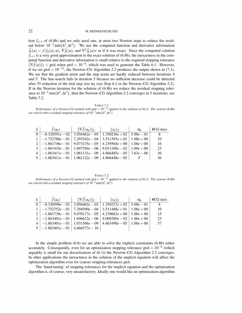
tion ~yi+1 of (6.8b) and we only need one, at most two Newton steps to reduce the resid-ual below 10−2 min{h2,∆t2}. We use the computed function and derivative informationfε(u) = f (yε(u),u), ∇ fε(u), and ∇2 fε(u)v as if it was exact. Since the computed solution~yi+1 is a very good approximation to the exact solution of (6.8b), the inexactness in the com-puted function and derivative information is small relative to the required stopping tolerance‖∇ f (u)‖2 < gtol when gtol = 10−8, which was used to generate the Table 6.1. However,if we set gtol = 10−12, the Newton–CG Algorithm 2.2 produces the output shown in (7.1).We see that the gradient norm and the step norm are hardly reduced between iterations 4and 5. The line-search fails in iteration 5 because no sufficient decrease could be detectedafter 55 reduction of the trial step size α5 (see Step 6.2 in the Newton–CG Algorithm 2.2).If in the Newton iteration for the solution of (6.8b) we reduce the residual stopping toler-ance to 10−5 min{h2,∆t2}, then the Newton–CG Algorithm 2.2 converges in 5 iterations, seeTable 7.2.
TABLE 7.1Performance of a Newton-CG method with gtol = 10−12 applied to the solution of (6.1). The systems (6.8b)
are solved with a residual stopping tolerance of 10−2 min{h2,∆t2}
k f (uk) ‖∇ f (uk)‖2 ‖sk‖2 αk #CG iters0 −8.320591e−02 3.056462e−03 1.350236e+02 5.00e−01 81 −1.752788e−01 7.293242e−04 3.511393e+01 1.00e+00 102 −1.861746e−01 9.073135e−05 4.239564e+00 1.00e+00 163 −1.863410e−01 1.697294e−06 9.011109e−02 1.00e+00 234 −1.863411e−01 1.061131e−09 4.866485e−05 7.63e−06 365 −1.863411e−01 1.061122e−09 4.866448e−05 F 36
TABLE 7.2Performance of a Newton-CG method with gtol = 10−12 applied to the solution of (6.1). The systems (6.8b)
are solved with a residual stopping tolerance of 10−5 min{h2,∆t2}
k f (uk) ‖∇ f (uk)‖2 ‖sk‖2 αk #CG iters0 −8.320590e−02 3.056462e−03 1.350237e+02 5.00e−01 81 −1.752752e−01 7.294590e−04 3.511488e+01 1.00e+00 102 −1.861738e−01 9.070177e−05 4.239663e+00 1.00e+00 153 −1.863401e−01 1.696622e−06 9.009389e−02 1.00e+00 234 −1.863401e−01 1.031566e−09 4.663490e−05 1.00e+00 375 −1.863401e−01 4.666573e−16
In the simple problem (6.8) we are able to solve the implicit constraints (6.8b) ratheraccurately. Consequently, even for an optimization stopping tolerance gtol = 10−8 (whicharguably is small for our discretization of (6.1)) the Newton–CG Algorithm 2.2 converges.In other applications the inexactness in the solution of the implicit equation will affect theoptimization algorithm even for coarser stopping tolerances gtol.
The ‘hand-tuning’ of stopping tolerances for the implicit equation and the optimizationalgorithm is, of course, very unsatisfactory. Ideally one would like an optimization algorithm
Numerical Solution of Implicitly Constrained Optimization Problems 23
that selects these automatically and allows more inexact and therefore less expensive solvesof the implicit equation at the beginning of the optimization iteration. One difficulty is thatone cannot compute the error in function and derivative information, but one can usually onlyprovide an asymptotic estimate of the form | fε(u)− f (u)|= O(ε).
There are approaches to handle inexact function and derivative information in optimiza-tion algorithms. For example, a general approach to this problem is presented in the book[28]. Additionally, Section 10.6 in [11] describes an approach to adjust the accuracy of func-tion values and derivatives in a trust-region method (see also the references in that section).Handling inexactness in optimization algorithms to increase the efficiency of the overall al-gorithm by using rough, inexpensive function and derivative information whenever possiblewhile maintaining the robustness of the optimization algorithm are important research prob-lems. Although approaches exist, more work remains to be done.
7.2. Constrainted Optimization. One may wonder why we have treated (1.1), (2.1),(2.2) as an implicitly constrained problem rather than using (2.3). Clearly the explicitly con-strained formulation (2.3) has several advantages:1) Often the problem (2.3) is well-posed, even if the constraint c(y,u) = 0 has multiple or nosolutions y for some u.2) The inexactness in function and derivative information that we have discussed in the pre-vious section and that arises out of the solution of c(y,u) = 0 for y is no longer an issue, sincey and u are both optimization variables in (2.3) and no implicit function has to be computed.3) Finally, optimization algorithms for (2.3), such as sequential quadratic programming (SQP)methods do not have to maintain feasibility throughout the iteration. This can lead to largegains in efficiency of SQP methods for (2.3) over Newton-type methods for the implicitlyconstrained problem (1.1), (2.1), (2.2).If possible, the formulation (2.3) should be chosen over (1.1), (2.1), (2.2). However, in manyapplications the number of y variables is so huge that it is infeasible to keep all in memory.This is for example the case for problems in which c(y,u)= 0 corresponds to the discretizationof time dependent partial differential equations in 3D. (Our 1D example problem in Section 6is a baby sibling of such problems.)
Constrained optimization problems of the type (2.3) can be solved using SQP methods.We mention a few ingredients of SQP methods for the solution of (2.3) with U =Rnu to pointout the relation between SQP methods for (2.3) and Newton-type methods for the implicitlyconstrained problem (1.1), (2.1), (2.2). More details on SQP methods can be found in [26].
SQP methods compute a solution of (2.3) with U = Rnu by solving a sequence ofquadratic programming (QP) problems
min(
∇y f (y,u)T
∇u f (y,u)
)T ( sysu
)+ 1
2
(sysu
)T (∇yyL(y,u,λ) ∇yuL(y,u,λ)∇uyL(y,u,λ) ∇uuL(y,u,λ)
)(sysu
),
s.t. cy(y,u)sy + cu(y,u)su =−c(y,u),(7.1)
where H is the Hessian of the Lagrangian (3.9),
H =
(∇yyL(y,u,λ) ∇yuL(y,u,λ)∇uyL(y,u,λ) ∇uuL(y,u,λ)
)or a replacement thereof. In so-called reduced SQP methods one uses
H =
(0 00 H
).
24 M. HEINKENSCHLOSS
The QP (7.1) is almost identical to the QPs (4.5) and (4.8) arising in Newton-type methodsfor the implicitly constrained problem (1.1), (2.1), (2.2). In the QPs (4.5) and (4.8), y = y(u)and λ = λ(u) and the right hand side of the constraint is c(y(u),u) = 0. This indicates thatone step of an SQP method for (2.3) may not be computationally more expensive than onestep of a Newton type method for (1.1), (2.1), (2.2). However, SQP methods profit from thedecoupling of the variables y and u and can be significantly more efficient than Newton typemethod for (1.1), (2.1), (2.2) because the latter compute iterates that are on the constraintmanifold.
8. Automatic Differentiation. In Section 6.3 we have ‘hand coded’ the gradient andHessian-vector multiplication for our example program (6.8). This can be very time consum-ing. Fortunately, one can use Automatic Differentiation in this process. ‘Automatic Differ-entiation (AD) is a set of techniques based on the mechanical application of the chain ruleto obtain derivatives of a function given as a computer program’ [1]. We have already comeacross AD in our discussion of checkpointing. For more information of how AD works werefer to [26, Sec. 8.2] and [14, 15]. The Community Portal for Automatic Differentiation [1]contains links to other AD resources, including software tools.
9. Differential Equation Constraints. In many applications, including our simplemodel problem (6.1), the governing equations are (partial) differential equations. After dis-cretization of the differential equations, one obtains a system of (nonlinear) algebraic equa-tions and the techniques discussed in this paper can be applied. However, it also possible toextend the techniques discussed in this paper so that hey are applicable to problems (1.1),(2.1), (2.2) posed in infinite dimensional function spaces. We refer to the books [8, 21] andreferences cited therein for optimization (optimal control) problems governed by ordinary dif-ferential equations and to the books [19, 30, 24] and references cited therein for optimization(optimal control) problems governed by partial differential equations.
REFERENCES
[1] Community portal for automatic differentiation. http://www.autodiff.org.[2] F. ABERGEL AND R. TEMAM, On some control problems in fluid mechanics, Theoretical and Computational
Fluid Dynamics, 1 (1990), pp. 303–325.[3] R. A. BARTLETT, Thyra linear operators and vectors: Overview of interfaces and support software for
the development and interoperability of abstract numerical algorithms, Tech. Rep. SAND 2007-5984,Sandia National Laboratories, 2007.
[4] R. A. BARTLETT, S. S. COLLIS, T. COFFEY, D. DAY, M. HEROUX, R. HOEKSTRA, R. HOOPER,R. PAWLOWSKI, E. PHIPPS, D. RIDZAL, A. SALINGER, H. THORNQUIST, AND J. WILLENBRING,ASC vertical integration milestone, Tech. Rep. SAND 2007-5839, Sandia National Laboratories, 2007.
[5] R. A. BARTLETT, B. G. VAN BLOEMEN WAANDERS, AND M. A. HEROUX, Vector reduc-tion/transformation operators, ACM Trans. Math. Software, 30 (2004), pp. 62–85.
[6] M. BERGGREN, Numerical solution of a flow-control problem: Vorticity reduction by dynamic boundaryaction, SIAM J. Scientific Computing, 19 (1998), pp. 829–860.
[7] D. P. BERTSEKAS, Nonlinear Programming, Athena Scientific, Belmont, Massachusetts, 1995.[8] A. BRYSON AND Y. HO, Applied Optimal Control, Hemisphere, New York, 1975.[9] J. M. BURGERS, Application of a model system to illustrate some points of the statistical theory of free
turbulence, Nederl. Akad. Wetensch., Proc., 43 (1940), pp. 2–12.[10] , A mathematical model illustrating the theory of turbulence, in Advances in Applied Mechanics,
R. von Mises and T. von Karman, eds., Academic Press Inc., New York, N. Y., 1948, pp. 171–199.[11] A. R. CONN, N. I. M. GOULD, AND P. L. TOINT, Trust–Region Methods, SIAM, Philadelphia, 2000.[12] J. E. DENNIS, JR. AND R. B. SCHNABEL, Numerical Methods for Nonlinear Equations and Unconstrained
Optimization, SIAM, Philadelphia, 1996.[13] M. S. GOCKENBACH, D. R. REYNOLDS, P. SHEN, AND W. W. SYMES, Efficient and automatic implemen-
tation of the adjoint state method, ACM Trans. Math. Softw., 28 (2002), pp. 22–44.[14] A. GRIEWANK, Evaluating Derivatives. Principles and Techniques of Algorithmic Differentiation, Frontiers
in Applied Mathematics, SIAM, Philadelphia, 2000.
Numerical Solution of Implicitly Constrained Optimization Problems 25
[15] , A mathematical view of automatic differentiation, in Acta Numerica 2003, A. Iserles, ed., CambridgeUniversity Press, Cambridge, London, New York, 2003, pp. 321–398.
[16] A. GRIEWANK AND A. WALTHER, Algorithm 799: revolve: An implementation of checkpointing for thereverse or adjoint mode of computational differentiation, ACM Trans. Math. Softw., 26 (2000), pp. 19–45.
[17] M. D. GUNZBURGER, Perspectives in Flow Control and Optimization, SIAM, Philadelphia, 2003.[18] M. HEINKENSCHLOSS AND L. N. VICENTE, An interface between optimization and application for the nu-
merical solution of optimal control problems, ACM Transactions on Mathematical Software, 25 (1999),pp. 157–190.
[19] M. HINZE, R. PINNAU, M. ULBRICH, AND S. ULBRICH, Optimization with Partial Differential Equations,vol. 23 of Mathematical Modelling, Theory and Applications, Springer Verlag, Heidelberg, New York,Berlin, 2009.
[20] M. HINZE, A. WALTHER, AND J. STERNBERG, An optimal memory-reduced procedure for calculatingadjoints of the instationary Navier-Stokes equations, Optimal Control Applications and Methods, 27(2006), pp. 19–40.
[21] J. JAHN, Introduction to the Theory of Nonlinear Optimization, Springer Verlag, Berlin, Heidelberg, NewYork, third ed., 2007.
[22] C. T. KELLEY, Iterative Methods for Optimization, SIAM, Philadelphia, 1999.[23] K. KUNISCH AND S. VOLKWEIN, Control of Burger’s equation by a reduced order approach using proper
orthogonal decomposition, Journal of Optimization Theory and Applications, 102 (1999), pp. 345–371.[24] J.-L. LIONS, Optimal Control of Systems Governed by Partial Differential Equations, Springer Verlag, Berlin,
Heidelberg, New York, 1971.[25] H. V. LY, K. D. MEASE, AND E. S. TITI, Distributed and boundary control of the viscous Burgers’ equation,
Numer. Funct. Anal. Optim., 18 (1997), pp. 143–188.[26] J. NOCEDAL AND S. J. WRIGHT, Numerical Optimization, Springer Verlag, Berlin, Heidelberg, New York,
second ed., 2006.[27] A. D. PADULA, Software Design for Simulation Driven Optimization, PhD thesis, Department of Computa-
tional and Applied Mathematics, Rice University, Houston, TX, 2005. Available as CAAM TR05–11.[28] E. POLAK, Optimization:Algorithms and Consistent Approximations, Applied Mathematical Sciences,
Vol. 124, Springer Verlag, Berlin, Heidelberg, New-York, 1997.[29] W. W. SYMES, A. D. PADULA, AND S. D. SCOTT, A software framework for the abstract expression of
coordinate-free linear algebra and optimization algorithms, tr05–12, Dept. of Computational and Ap-plied Mathematics, Rice University, Houston, Texas, 2005.
[30] F. TROLTZSCH, Optimal Control of Partial Differential Equations: Theory, Methods and Applications,vol. 112 of Graduate Studies in Mathematics, American Mathematical Society, Providence, RI, 2010.
[31] S. VOLKWEIN, Distributed control problems for the Burgers equation, Comput. Optim. Appl., 18 (2001),pp. 115–140.