numerical solution of riemann{hilbert problems: · pdf filenumerical solution of...
TRANSCRIPT

Report no. 09/9
Numerical solution of Riemann–Hilbert problems: Painleve II
Sheehan Olver
Abstract We describe a new, spectrally accurate method for solving matrix-
valued Riemann–Hilbert problems numerically. The effectiveness of this ap-
proach is demonstrated by computing solutions to the homogeneous Painleve
II equation. This can be used to relate initial conditions with asymptotic be-
haviour.
Keywords Riemann–Hilbert problems, spectral methods, collocation meth-
ods, Painleve transcendents.
Oxford University Mathematical Institute
Numerical Analysis Group
24-29 St Giles’Oxford, England OX1 3LB
E-mail: [email protected] August, 2010

1. Introduction
Riemann–Hilbert problems occupy an important place in applied analysis. They have
been used to derive asymptotics for nonlinear differential equations such as the Painleve
transcendents [15], the nonlinear Schrodinger equation and the KdV equation [1], as well
as orthogonal polynomials and random matrices [9]. Whereas the originating equations are
nonlinear, Riemann–Hilbert problems are linear. A key aspect to their effectiveness is that
they can be deformed in the complex plane to turn oscillations into exponential decay, so that
asymptotics can be derived. This is known as nonlinear steepest descent [11], as it is much
like the classical theory of steepest descent for oscillatory integrals. Thus Riemann–Hilbert
formulations can loosely be viewed as a nonlinear counterpart to the integral representations
that are known for many important linear differential equations; such as the Airy equation,
hypergeometric equations [2], wave equation and heat equation.
Integral representations have another important use, in addition to the derivation of
asymptotics: numerical computation through quadrature. Indeed, they have been used to
great effect for computing Airy functions and Bessel functions [16], which, in a certain sense,
are linear analogues of Painleve transcendents. The aim of this paper is to demonstrate that
Riemann–Hilbert problems share this property with integral representations: they can also
be used to compute solutions to the associated equations numerically.
A Riemann–Hilbert problem is the problem of finding a function that is analytic every-
where in the complex plane except along a given curve, on which it has a prescribed jump.
This can be written more precisely as
Problem 1.1 [20] Given an oriented curve Γ ⊂ C and a jump matrix G : Γ→ C2×2, find a
bounded function Φ : C\Γ→ C2×2 which is analytic everywhere except on Γ such that
Φ+(z) = Φ−(z)G(z) for z ∈ Γ and
Φ(∞) = I,
where Φ+ denotes the limit of Φ as z approaches Γ from the left, and Φ− denotes the limit
of Φ as z approaches Γ from the right and Φ(∞) = lim|z|→∞Φ(z).
To demonstrate the numerical approach, we will focus on the Painleve II transcendent,
though the techniques developed are generalizable for other Riemann–Hilbert problems. The
Painleve II equation is
u′′ = xu+ 2u3 − α, (1.1)
where α is a complex parameter. For simplicity, we will take α = 0. From this differential
equation, an equivalent Riemann–Hilbert formulation is derived by finding a Lax pair rep-
resentation, which in turn is uniquely specified by behaviour along Stokes’ lines. This can
then be rephrased as a Riemann–Hilbert problem [15].
1

�1 s2e
− 8i3 z3−2ixz
1
�
�1 −s1e
− 8i3 z3−2ixz
1
� �1 −s3e
− 8i3 z3−2ixz
1
�
�1
s1e8i3 z3+2ixz 1
��1
s3e8i3 z3+2ixz 1
�
�1
−s2e8i3 z3+2ixz 1
�
Figure 1: The curve and jump matrix for the Painleve II Riemann–Hilbert problem.
As explained in [18], the curve Γ in the Riemann–Hilbert problem for the homogeneous
Painleve II equation consists of six rays eminating from the origin (see Figure 1):
Γ = Γ1 ∪ · · · ∪ Γ6
where Γκ ={z ∈ C : arg z = π
(1
6+κ− 1
3
)}.
The jump function has a different definition depending on which ray Γκ that z lies on:
G(x; z) =
(1 sκe−
8i3 z
3−2ixz
1
)κ even and z ∈ Γκ,
(1
sκe8i3 z
3+2ixz 1
)κ odd and z ∈ Γκ.
Instead of imposing initial conditions, we choose Stokes’ constants s1, s2 and s3 which satisfy
the following compatibility condition:
s1 − s2 + s3 + s1s2s3 = 0, (1.2)
from which the remaining Stokes’ constants are defined as
s4 = −s1, s5 = −s2 and s6 = −s3.
2

Once we have found a function Φ(x; z) that satisfies the Painleve II Riemann–Hilbert
problem, a solution to (1.1) is
u(x) = limz→∞ 2zΦ(12)(x; z).
If u does not have a pole at x, then (1.2) is sufficient to ensure a unique solution to the
Riemann–Hilbert problem [15]. As in the integral representation of the Airy function, the
original variable x has been reduced to a parameter.
By moving from the original differential equation to Problem 1.1, we have transformed
a nonlinear problem to a linear problem, ignoring the boundary condition at ∞. We can
rephrase the problem so that it is completely linear: define
U = Φ− I;
thence,
LU = U+ − U−G = G− I and U(∞) = 0. (1.3)
Now the operator L is linear, from the space of functions analytic off Γ and which decay at
∞ to the space of functions defined on Γ.
Consider for the moment the following simple and scalar Riemann–Hilbert problem:
Problem 1.2 Given an oriented curve Γ ⊂ C and a function f : Γ → C which is Holder-
continuous on each smooth segment of Γ, find a function ψ : C\Γ → C which is analytic
everywhere except on Γ such that
ψ+(z)− ψ−(z) = f(z) for z ∈ Γ and ψ(∞) = 0.
For analysts, solving this problem is a trivial application of Plemelj’s lemma [20], and
the solution is the Cauchy transform:
ψ(z) = CΓf(z) =1
iπ
∫
Γ
f(t)
t− z dt for z /∈ Γ. (1.4)
(When Γ is clear from context, we use the notation C.) However, by rewritting Problem 1.2
as an integral, we have, in a certain sense, moved backwards: the functions in Problem 1.2
are bounded (and, in the Painleve case, analytic), whereas (1.4) has introduced a singularity
that must somehow be dealt with. Thus the approach taken in [25] was to apply Plemelj’s
lemma in reverse; i.e., compute (1.4) numerically by rewriting it as Problem 1.2. This can
be accomplished efficiently using the FFT when Γ is a circle, interval, ray or combination
of multiple such curves, as reviewed in Section 3. Moreover, this approach allows us to also
compute the left and right limits of the Cauchy transform C±, which we require.
The importance of the operator C is that it uniquely maps any Holder-continuous function
defined on Γ to an analytic function defined off Γ [20]. This still holds true when it is a
matrix-valued function, in a component-wise manner. Moreover, under certain conditions
3
which are satisfied in our case, this map is one-to-one. In other words, for a function V
defined on Γ, if
LCV = C+V − (C−V )G = G− I, (1.5)
it follows that Ψ = CV + I satisfies all the conditions of Problem 1.1. Moreover, LC maps
the space of functions which are Holder-continuous on the segments of Γ to itself.
Our numerical approach is to impose (1.5) at a sequence of points lying on Γ:
Algorithm 1.3
1: Represent
V (z) =
V1(z) z ∈ Γ1...
V6(z) z ∈ Γ6
for Vκ(z) =
pκ(z)v
(11)κ pκ(z)v
(12)κ
pκ(z)v(21)κ pκ(z)v
(22)κ
,
where pκ = (pκ1, . . . , pκn) denotes a basis for functions defined on Γκ and v(ij)κ =
(v
(ij)κ1 , . . . , v
(ij)κn
)>are unknowns in Cn;
2: For collocation points zκ = (zκ1, . . . , zκn)> in Γκ, compute the Cauchy transform for the
chosen basis at the points z1, . . . ,z6;
3: Determine v(ij)κ by solving the 24n× 24n linear system
LCV (z1) = G(z1)− I,...
LCV (z6) = G(z6)− I;
(1.6)
4: Convert(v
(12)1 , . . . ,v
(12)6
)>to un(x), which approximates u(x).
The next four sections correspond to each of the steps of Algorithm 1.3. In Section 2,
we use mapped Chebyshev polynomials as our basis and mapped Chebyshev–Lobatto points
as our collocation points. In Section 3, we derive an expression for the Cauchy transform
of this basis in closed form. However, the junction point zero is included as a collocation
point, at which the Cauchy transform generically blows up. Therefore, the system (1.6), as
written, cannot be used. However, the six unbounded Cauchy transforms CΓ1V1, . . . , CΓ6V6
can sum in such away that the unbounded terms cancel, leaving only bounded terms. We
can determine the remaining bounded terms for each Cauchy transform, which is what we
will use in the linear system as its value at zero. In Section 4, we construct the true form of
(1.6). Whereas Algorithm 1.3 suggests that we will need to solve a 24n× 24n linear system,
we will find that the degree of the linear system can be reduced 6(n− 1)× 6(n− 1) by using
a priori information about the solution. In Theorem 4.3 we prove that our choice of value of
4

the Cauchy transforms at the junction point is justified subject to a condition on the Stokes’
multipliers s1, s2, s3: it automatically implies that the unbounded terms do indeed cancel
and the approximation does solve the conditions of (1.6). Finally, by integrating over Γ we
can convert the solution to the Riemann–Hilbert problem to a solution to the homogenous
Painleve II equation, as explained in Section 5.
There are approaches for the computation of solutions to other Riemann–Hilbert prob-
lems. The conjugation method [30] can be used to solve a nonlinear Riemann–Hilbert prob-
lem on the unit circle related to conformal mapping. This has been generalized to multiple
circles [29, 31], but not to intervals or curves like our Γ. Another approach applicable to
smooth closed curves is based on solving integral equations [21]. An approach which is sim-
ilar to ours was used in [13], where a Riemann–Hilbert problem associated with the sine
kernel Fredholm determinant (which has applications in random matrix theory) was solved
by reducing the equation to a singular integral equation, precisely as in (1.5). However, in
this approach the endpoints and junction points of the jump curve were avoided, and hence
exponentially many sample points were required near the endpoints to simulate boundedness
of the solution. On the other hand, in our approach we ensure that the junction points are
included in the collocation system, thus we automatically have a bounded solution and this
inefficiency is avoided.
Remark : Based on the method presented here, a Mathematica package, RHPackage,
has subsequently been developed for solving general Riemann–Hilbert problems [23]. How
the current approach is adaptable to general Riemann–Hilbert problems is described in [24].
Included in the package is an implementation of the method described in this paper for
computing Painleve II, which is more optimized than the general routine. We use this
implementation in the numerical results below.
2. Choice of basis
Each curve Γκ is a ray in the complex plane. An oft-used technique from spectral
methods, which we employ, is to represent a function defined on a ray by mapping it to a
function defined on the unit interval. Indeed, we can conformally map the unit interval to
Γκ using the map
Hκ(t) = eiπ( 16+κ−1
3 ) t+ 1
1− t .
(The map typically used is LHκ(t) for some constant L [7]. We fix L = 1 for simplicity.)
On the unit interval, the natural representation for functions is Chebyshev series.
5
Definition 2.1 For a fixed integer n ≥ 2, define the n Chebyshev–Lobatto points as
χ =(−1, cosπ
(1− 1
n− 1
), . . . , cos
π
n− 1, 1)>,
We can efficiently represent a function defined on the interval by its values at χ:
f = f(χ).
By taking an appropriately scaled discrete cosine transform of f , which we denote D, we
obtain the Chebyshev polynomial which interpolates f at χ:
e(t)>f = (T0(t), . . . , Tn−1(t))Df ,
where Tk are the Chebyshev polynomials of the first kind [2]. Alternatively, the barycentric
formula can be used [5].
In practice, f will vanish at t = +1, as this will correspond to z =∞. We want our basis
to capture that fact, so when we map the basis back to the half ray, it decays at infinity
and the Cauchy transform is well-defined. Therefore, we replace the basis T0, . . . , Tn−1 with
T0−1, . . . , Tn−1−1. Fortunately, since f vanishes at 1, we know that (1, . . . , 1)Df = f(1) = 0
and therefore
e(t)>f = (T0(t)− 1, . . . , Tn−1(t)− 1)Df .
Definition 2.2 For a vector x = (x1, . . . , xn)>, the notation x denotes x with its last entry
removed: x = (x1, . . . , xn−1)>.
Using the map Hκ and the fact that every function r we consider vanishes at ∞, we can
then represent a function r defined on Γκ by its values at n− 1 mapped Chebyshev–Lobatto
points:
rκ = r(zκ) for zκ = Hκ(χ).
The values at the points zκ = Hκ(χ) are rκ =(rκ0
)and the basis is
TΓκk (z) = Tk(H
−1κ (z))− 1.
We also define the n×(n−1) transform matrix for this truncated vector as D by the formula
Drκ = Drκ.Then the function
e(H−1κ (z))>rκ =
(TΓκ
0 (z), . . . , TΓκn−1(z)
)>Drκ
interpolates r at the points zκ. This is referred to as a rational Chebyshev interpolant [7].
6
Thus we approximate a function r which is smooth along each Γκ by the function
e(H−11 (z))>r1 z ∈ Γ1,
...e(H−1
6 (z))>r6 z ∈ Γ6.
In the notation of Algorithm 1.3 we use the basis whose elements are one at a point in zκand zero at every other point:
pκj(z) = e(H−1κ (z))>ej .
Then the coefficients v(ij)κ correspond to function values at the points zκ.
3. Computing the Cauchy transform over Γ
Our goal in this section is to construct Cauchy matrices C±, corresponding to the eval-
uation of the Cauchy transform C±Γ1along Γ1. If r1 = r(z1), consider
C±r1 =? C±e(H−1
1 (z1))>r1 =(C±Γ1
TΓ10 (z1), . . . , C±Γ1
TΓ1n−1(z1)
)Dr1.
This definition will suffice for every row of the matrix other than the first, provided we can
compute the left and right limits of the Cauchy transform for the chosen basis. On the other
hand, since the Cauchy transform is unbounded at zero, this definition fails for the first row,
and an alternative definition must be used.
We also want matrices C2, . . . , C6 corresponding to the evaluation of CΓ1 along Γ2, . . . ,Γ6:
Cκr1 =? (CΓ1T
Γ10 (zκ), . . . , CΓ1T
Γ1n−1(zκ)
)Dr1.
The first row of these definitions must also be altered. We will see that these matrices aresufficient to represent the Cauchy transform over the other curves Γ2, . . . ,Γ6 as well, due tosymmetry.
In order to construct these matrices, we must compute the Cauchy transform for our
basis, which can be written in terms of the Cauchy transform of the Chebyshev polynomials
over the unit interval.
Computation of the Cauchy transform over the unit interval
We have an expression for C(−1,1)Tk in closed form. This expression is derived by mapping
the interval to the unit circle, using the Joukowsky map and its inverses:
Definition 3.1 The Joukowsky map
T (z) =1
2
(z +
1
z
)
7

maps the interior and exterior of the unit circle to C\[−1, 1]. Thus it has two inverses defined
in C\[−1, 1]:
T−1± (t) = t∓
√t− 1
√t+ 1.
T−1+ and T−1
− map C\[−1, 1] to the interior and exterior of the circle, respectively. Since T±
each have a branch cut along [−1, 1], we need two additional inverses:
T−1↑ (t) = t+ i
√1− t
√1 + t and T−1
↓ (t) = t− i√
1− t√
1 + t.
These map [−1, 1] to the upper and lower half of the unit circle, respectively, and are analytic
along the interval.
Using these maps, we obtain the following formulæ:
Theorem 3.2 Define
µm(z) =
bm+12 c∑
j=1
z2j−1
2j − 1, ψ0(z) =
2
iπarctanh z,
ψm(z) = zm[ψ0(z)− 2
iπ
{µ−m−1(z) for m < 0µm(1/z) for m > 0
].
Then
C(−1,1)Tk(t) = −1
2
[ψk(T
−1+ (t)) + ψ−k(T
−1+ (t))
],
C(−1,1)Tk(t) ∼t→−1
− 1
2iπ(−1)k [log(−t− 1)− log 2] +
1
iπ(−1)k [µk−1(−1) + µk(−1)] , (3.1)
C(−1,1)Tk(t) ∼t→1
1
2iπ[log(t− 1)− log 2] +
1
iπ[µk−1(1) + µk(1)] , (3.2)
and, for t ∈ (−1, 1),
C+(−1,1)Tk(t) = −1
2
[ψk(T
−1↓ (t)) + ψ−k(T
−1↓ (t))
],
C−(−1,1)Tk(t) = −1
2
[ψk(T
−1↑ (t)) + ψ−k(T
−1↑ (t))
].
Proof :
This theorem is a simplification of Theorem 6 in [25]. Take the definition above of ψm(z)
for |z| < 1, and define for |z| > 1:
ψ0(z) =2
iπarctanh
1
z,
8

ψm(z) = zm[ψ0(z)− 2
iπ
{µ−m−1(z) for m < 0µm(1/z) for m > 0
].
From [25] we have
CTk(x) = −1
4
[ψk(T
−1+ (t)) + ψk(T
−1− (t)) + ψ−k(T
−1+ (t)) + ψ−k(T
−1− (t))
]. (3.3)
We now sketch a proof of this result. The function ψm is defined so that, for |z| = 1,
ψ+m(z)− ψ−m(z) = zm sgn arg z and ψm(∞) = 0.
For m = 0 this follows from the definition of arctanh. For m > 0, ψm is equal to zmψ0(z)
with the growth at∞ subtracted out, determined by the necessary terms of the Taylor series
of arctanh: µm. For m < 0, ψm is equal to zmψ0(z) with the pole at zero subtracted out to
ensure analyticity at zero, also determined from the Taylor series.
If g(z) = −f(T (z)) sgn arg z and ψ is the Cauchy transform of g over the unit circle,
ψ = C{z:|z|=1}g, then
C(−1,1)f(t) =ψ(T+(t)) + ψ(T−(t))
2.
This follows since
C+(−1,1)f(t)− C−(−1,1)f(t) =
ψ+(T↓(t)) + ψ−(T↑(t))− ψ+(T↑(t))− ψ−(T↓(t))
2= f(t)
and
ψ(T+(∞)) + ψ(T−(∞)) = ψ(0) = g0 = 0,
as g is symmetric. This proves (3.3), since Tk(T (z)) = 12
[zk + z−k
].
We can simplify (3.3). Note that T−1− (t) = 1
T−1+ (t), therefore ψ0(T−1
− (t)) = ψ0(T−1+ (t)).
Furthermore, for k > 0
ψk(T−1− (t)) = T−1
+ (t)−k[ψ0(T−1
+ (t))− 2
iπµk(T−1
+ (t))]
= ψ−k(T−1+ (t)) +
{12k k odd0 k even
and
ψ−k(T−1− (t)) = ψk(T
−1+ (t))−
{12k k odd0 k even
.
It follows that
ψk(T−1− (t)) + ψ−k(T
−1− (t)) = ψk(T
−1+ (t)) + ψ−k(T
−1+ (t)).
9

The asymptotic behaviour at the endpoints was shown in [25]. The expression for C±Tkfollows from the expression for CTk and the fact that, for z ∈ (−1, 1), limε→0+ T+(z + iε) =
T−1↓ (t) and limε→0+ T+(z − iε) = T−1
↑ (t).
Q.E.D.
Remark : One approach to computing ψm is to use the definition above with high precision
arithmetic (which is necessary as the definition is chosen precisely to cancel terms in the Tay-
lor series). Another approach [25] is to rewrite the series in terms of the Lerch transcendent
function [4], and use the method developed in [3], or the built-in Mathematica routine.
A fast, numerically stable and accurate approach is to compute ψm by writing it in terms
of the Hypergeometric function, and then use a stable recurrence relation to subsequently
obtain ψm+1, ψm+2, . . . [24].
Computation of the Cauchy transform over a half ray
Similar to the development in [25], we can write CΓκ in terms of C(−1,1): if f(t) = r(Hκ(t))
and Φ = C(−1,1)f , then
CΓκr(z) = Φ(H−1κ (z))− Φ+(1).
This is easily confirmed by looking at the behaviour as z approaches Γκ from the left and
right:
C+Γκr(z)− C−Γκr(z) = Φ+(H−1
κ (z))− Φ−(H−1κ (z)) = f(H−1
κ (z)) = r(z) and
limz→∞ CΓκr(z) = lim
z→∞Φ(H−1κ (z))− Φ+(1) = lim
t→1Φ(t)− Φ+(1) = 0,
since
Φ+(1)− Φ−(1) = r(∞) = 0.
Using this formula, we can derive an expression for CΓκTΓκk :
CΓκTΓκk (z) = C(−1,1)[Tk − 1](H−1
κ (z))− C+(−1,1)[Tk − 1](1).
The unbounded terms of C(−1,1)[Tk − 1](t) are cancelled as t→ 1, therefore we are left with
C+(−1,1)[Tk − 1](1) =
1
iπ[µk−1(1) + µk(1)] .
We thus obtain
CΓκTΓκk (z) = −1
2
[ψk(T
−1+ (H−1
κ (z))) + ψ−k(T−1+ (H−1
κ (z)))− 2ψ0(T−1+ (H−1
κ (z)))]
10

− 1
iπ[µk−1(1) + µk(1)] . (3.4)
Behaviour at zero
The expression (3.4) explodes at zero. We describe this behaviour, in order to choose a
value to assign for the first row of the Cauchy matrices, corresponding to evaluation at zero.
From Theorem 3.2 and (3.4) we have
CΓκTΓκk (z) ∼
z→0
1− (−1)k
2iπ
[log(−H−1
κ (z)− 1)− log 2]
+(−1)k
iπ[µk−1(−1) + µk(−1)]− 1
iπ[µk−1(1) + µk(1)] .
From the expression
H−1κ (z) =
z − eiπ( 16+κ−1
3 )
z + eiπ( 16+κ−1
3 )
we find that
H−1κ (z) = −1 + 2e−iπ( 1
6+κ−13 )z +O
(z2).
Therefore
CΓκTΓκk (z) ∼ 1
2iπ
[1− (−1)k
] [log(−2e−iπ( 1
6+κ−13 )z
)− log 2
]
+(−1)k
iπ[µk−1(−1) + µk(−1)]− 1
iπ[µk−1(1) + µk(1)]
=1− (−1)k
2iπlog |z|+ 1− (−1)k
2iπi arg
(−e−iπ( 1
6+κ−13 )z
)
+(−1)k
iπ[µk−1(−1) + µk(−1)]− 1
iπ[µk−1(1) + µk(1)] . (3.5)
Our choice for the value of the Cauchy transform at zero is this expression with the term
that grows like log |z| dropped. Note that it depends on the angle at which we approachzero.
Constructing Cauchy matrices
We can now construct the Cauchy matrices. We begin with C+. Note in (3.5) that the
term dependent on the angle is, for the limit as z approaches Γ1 from the left,
limε→0+
arg(−e−iπ6 ei(π6 +ε)
)= lim
ε→0+arg
(ei(−π+ε)
)= −π.
Thus we define
C+ =(ϕ+
0 (χ), . . . , ϕ+n−1(χ)
)D
11

for
ϕ+k (t) = −1
2
[ψk(T
−1↓ (t)) + ψ−k(T
−1↓ (t))− 2ψ0(T−1
↓ (t))]− µk−1(1) + µk(1)
iπ,
ϕ+k (−1) = −1− (−1)k
2+ (−1)k
µk−1(−1) + µk(−1)
iπ− µk−1(1) + µk(1)
iπ.
Similarly, we can define C− via
C− =(ϕ−0 (χ), . . . , ϕ−n−1(χ)
)D
for
ϕ−k (t) = −1
2
[ψk(T
−1↑ (t)) + ψ−k(T
−1↑ (t))− 2ψ0(T−1
↑ (t))]− µk−1(1) + µk(1)
iπ,
ϕ−k (−1) =1− (−1)k
2+ (−1)k
µk−1(−1) + µk(−1)
iπ− µk−1(1) + µk(1)
iπ.
Finally, we define Cγ , corresponding to evaluating CΓ1 along Γγ for γ = 2, . . . , 6. Now z
in (3.5) lies in Γγ , hence
arg(−e−iπ6 z
)= arg
(−e−iπ6 eiπ( 1
6+γ−13 ))
= πγ − 4
3.
Therefore we define
Cγ =(ϕ0,γ(H−1
1 (zγ)), . . . , ϕn−1,γ(H−11 (zγ))
)D
where
ϕk,γ(t) = −1
2
[ψk(T
−1+ (t)) + ψ−k(T
−1+ (t))− 2ψ0(T−1
+ (t))]− µk−1(1) + µk(1)
iπ,
ϕk,γ(−1) = (1− (−1)k)(γ
6− 2
3
)+ (−1)k
µk−1(−1) + µk(−1)
iπ− µk−1(1) + µk(1)
iπ.
Ostensibly we would need to redo these calculations for each Γκ to compute CΓκ . How-
ever, C is invariant under rotation. Therefore (ignoring the unboundedness at zero)
C±rκ = C±Γκe(H−1κ (zκ))>rκ,
Cγ−κ+1 mod 6rκ = C±Γκe(H−1κ (zγ))>rκ.
Since the Cauchy transform of a function r(z) defined on Γ is
CΓr(z) = CΓ1r(z) + · · ·+ CΓ6r(z),
we obtain
C±Γ r(z1) ≈ C±Γ1e(H−1
1 (z1))>r1 + CΓ2e(H−12 (z1))>r2 + · · ·+ CΓ6e(H−1
6 (z1))>r6
12
≈ C±r1 + C6r2 + C5r3 + · · ·+ C2r6, (3.6)
C±Γ r(z2) ≈ C2r1 + C±r2 + C6r3 + · · ·+ C3r6,
...
C±Γ r(z6) ≈ C6r1 + · · ·C2r5 + C±r6.
4. Constructing the linear system
We now use the matrices C±, C2, . . . , C6 to construct the linear system (1.6). We repre-
sent U via the definition
U (ij) = CV (ij) =6∑
κ=1
CΓκV(ij)κ ≈
6∑
κ=1
CΓκe(H−1κ (z))>v(ij)
κ .
Given v(ij)1 , . . . ,v
(ij)6 , we can determine the the approximation of C±V (ij) at the points
z1, . . . , z6 using (3.6):
c±,(ij)1 = C±v
(ij)1 + C6v
(ij)2 + · · ·+ C2v
(ij)6 ,
...
c±,(ij)6 = C6v
(ij)1 + · · ·+ C2v
(ij)5 + C±v
(ij)6 .
Hence we determine v(ij)1 , . . . ,v
(ij)6 by solving the 24(n− 1)× 24(n− 1) linear system
c+1 − c−1 G(z1) = G(z1)− I (4.1)
...
c+6 − c−6 G(z6) = G(z6)− I.
Here we take
G(zk) =
(G(11)(zk) G(12)(zk)
G(21)(zk) G(22)(zk)
)
and define multiplication of two matrices whose entries are vectors as
(c(11) c(12)
c(21) c(22)
)(g(11) g(12)
g(21) g(22)
)
=
diag
(c(11)
)g(11) + diag
(c(12)
)g(21) diag
(c(11)
)g(12) + diag
(c(12)
)g(22)
diag(c(21)
)g(11) + diag
(c(22)
)g(21) diag
(c(21)
)g(12) + diag
(c(22)
)g(22)
.
13

Reducing the dimension of the system
We can derive properties of the solution which will allow us to decrease the dimension
of the linear system. Now consider the case where γ is odd. Since CΓκV(ij)κ is analytic off
Γκ, and, by definition, C+Γγr − C−Γγr = r along Γγ , we obtain (here the ± refer to the limits
to a point in Γγ)
U (ij)+ − U (ij)− =6∑
κ=1
(C+Γκ− C−Γκ)V (ij)
κ = (C+Γγ− C−Γγ )V (ij)
γ = V (ij)γ
along Γγ . This implies that
LCV = U+ − U−G =
(U (11)+ U (12)+
U (21)+ U (22)+
)−(U (11)− U (12)−
U (21)− U (22)−
)(1
sγe8i3 z
3+2ixz 1
)
=
U
(11)+ − U (11)− − U (12)−sγe8i3 z
3+2ixz U (12)+ − U (12)−
U (21)+ − U (21)− − U (22)−sγe8i3 z
3+2ixz U (22)+ − U (22)−
=
V
(11)γ − sγe
8i3 z
3+2ixzC−V (12) V(12)γ
V(21)γ − sγe
8i3 z
3+2ixzC−V (22) V(22)γ
.
On the other hand, the right-hand side is
G− I =
(0 0
sγe8i3 z
3+2ixz 0
).
Therefore, we trivially obtain that 0 = V(12)γ = V
(22)γ , or in other words, the contribution to
U (12) and U (22) from Γγ is zero and we take 0 = v(12)γ = v
(22)γ .
Similarly, when γ is even we obtain
LCV =
V
(11)γ V
(12)γ − sγe−
8i3 z
3−2ixzC−V (11)
V(21)γ V
(22)γ − sγe−
8i3 z
3−2ixzC−V (21)
=
(0 sγe−
8i3 z
3−2ixz
0 0
).
Therefore, we take 0 = v(11)γ = v
(21)γ . In other words, V
(11)γ and V
(21)γ are only nonzero for
odd γ, V(21)γ and V
(22)γ are only nonzero for even γ.
Finally, we note that the top rows of V1, . . . , V6 are completely independent of the bottomrows.
Using these simplifications, we can reduce the dimension of (4.1), from one 24(n− 1)×24(n− 1) system to two 6(n− 1)× 6(n− 1) systems. The first system is for the unknowns
14

associated with the (11) and (12) entries of V :
v(11)1 − s1diag (e
8i3 z
31+2ixz1)
[C6v
(12)2 + C4v
(12)4 + C2v
(12)6
]= 0,
v(12)2 − s2diag (e−
8i3 z
32−2ixz2)
[C2v
(11)1 + C6v
(11)3 + C4v
(11)5
]= s2e−
8i3 z
32−2ixz2 ,
v(11)3 − s3diag (e
8i3 z
33+2ixz3)
[C2v
(12)2 + C6v
(12)4 + C4v
(12)6
]= 0,
v(12)4 + s1diag (e−
8i3 z
34−2ixz4)
[C4v
(11)1 + C2v
(11)3 + C6v
(11)5
]= −s1e−
8i3 z
34−2ixz4 ,
v(11)5 + s2diag (e
8i3 z
35+2ixz5)
[C4v
(12)2 + C2v
(12)4 + C6v
(12)6
]= 0,
v(12)6 + s3diag (e−
8i3 z
36−2ixz6)
[C6v
(11)1 + C4v
(11)3 + C2v
(11)5
]= −s3e−
8i3 z
36−2ixz6 .
The second system is for the unknowns associated with the (21) and (22) entries:
v(21)1 − s1diag (e
8i3 z
31+2ixz1)
[C6v
(22)2 + C4v
(22)4 + C2v
(22)6
]= s1e
8i3 z
31+2ixz1 ,
v(22)2 − s2diag (e−
8i3 z
32−2ixz2)
[C2v
(21)1 + C6v
(21)3 + C4v
(21)5
]= 0,
v(21)3 − s3diag (e
8i3 z
33+2ixz3)
[C2v
(22)2 + C6v
(22)4 + C4v
(22)6
]= s3e
8i3 z
33+2ixz3 ,
v(22)4 + s1diag (e−
8i3 z
34−2ixz4)
[C4v
(21)1 + C2v
(21)3 + C6v
(21)5
]= 0,
v(21)5 + s2diag (e
8i3 z
35+2ixz5)
[C4v
(22)2 + C2v
(22)4 + C6v
(22)6
]= −s2e
8i3 z
35+2ixz5 ,
v(22)6 + s3diag (e−
8i3 z
36−2ixz6)
[C6v
(21)1 + C4v
(21)3 + C2v
(21)5
]= 0.
Note that the left-hand side of both linear systems are the same, thus most of the computation
can be reused.
Though we have described how to construct C± and Cγ for odd γ, we only require the
computation of C2, C4 and C6. This simplification will not necessarily be possible for other
Riemann–Hilbert problems.
For the conversion from the Riemann–Hilbert problem to the value of the solution to
Painleve II at x, we require the (12) entry of Φ, which is also the (12) entry of U . Thus
we need only solve the first linear system. Assuming the linear system is nonsingular, we
denote the solution vectors for a given n as v(ij),nκ , unless n is implied by context. The
15

50 100 150n
10-10
10-7
10-4
0.1
100
50 100 150n
10-8
10-5
0.01
10
Figure 2: The convergence of the first entry of the solution vectors (first graph) and the ap-proximation of un compared to u200 (right graph) for x = 0 (plain), 6 (dashed), 8 (dotted) and i(thick).
approximations of V and U are
V nκ (z) =
e(H−1
κ (z))>v(11),nκ e(H−1
κ (z))>v(12),nκ
e(H−1κ (z))>v
(21),nκ e(H−1
κ (z))>v(22),nκ
and
Un(z) = CΓ1Vn
1 (z) + · · ·+ CΓ6Vn
6 (z),
where the Cauchy transforms can be computed as in Section 3.
As an example, consider the choice of constants (s1, s2, s3) = (1 + i,−2, 1 − i). Since
s1 = s3, we know that the corresponding solution to Painleve II is real on the real axis [15].
To demonstrate the rate of convergence, in Figure 2 we compare the first entry of solution
vectors (which corresponds to the value at zero along each Γκ) for consecutive choices of n:
∥∥∥∥∥∥∥∥∥∥∥∥∥∥∥∥∥∥∥∥∥∥∥∥∥
e>1
(v
(11),n1 − v(11),n+1
1
)
e>1
(v
(11),n3 − v(11),n+1
3
)
e>1
(v
(11),n5 − v(11),n+1
5
)
e>1
(v
(12),n2 − v(12),n+1
2
)
e>1
(v
(12),n4 − v(12),n+1
4
)
e>1
(v
(12),n6 − v(12),n+1
6
)
∥∥∥∥∥∥∥∥∥∥∥∥∥∥∥∥∥∥∥∥∥∥∥∥∥∞
.
As can be seen, these values converges spectrally fast, including for complex x, though the
rate of convergence and stability degenerates as x becomes large.
Properties of the solution
In the previous example, the linear system was always nonsingular. We cannot expect
that this is always the case, as if x corresponds to a pole of the solution u(x), then the
16

corresponding Riemann–Hilbert problem itself is not solvable. We do, however know the
following:
Theorem 4.1 The two linear systems are solvable for sufficiently small (s1, s2, s3).
Proof : When (s1, s2, s3) = (0, 0, 0), the matrix associated with each linear system is simply
an identity operator. Thus continuity of eigenvalues proves the result. Q.E.D.
In the construction of Cκ, we determined the value at zero by assuming the solution was
bounded. This will be true when the hypotheses of the following lemma are satisfied:
Lemma 4.2 Suppose that the linear system is nonsingular and that the computed solutions
values at zero sum to zero:
0 = e>1
[v
(11)1 + v
(11)3 + v
(11)5
], 0 = e>1
[v
(12)2 + v
(12)4 + v
(12)6
],
0 = e>1
[v
(21)1 + v
(21)3 + v
(21)5
], 0 = e>1
[v
(22)2 + v
(22)4 + v
(22)6
].
Then the solution Un(z) is analytic everywhere off Γ, bounded at zero and satisfies the
relationship (1.5) at the points z1, . . . ,z6.
Proof :
The first part of the lemma follows since CΓk is analytic off Γk.
For the second part of the lemma, we consider the (11) entry, as the proof for other
entries is the same. The only possible blow-up from the Cauchy transforms is at zero. From
(3.5) we find that the behaviour at zero is
U (11),n(z) = CΓ1e(H−11 (z))>v
(11)1 + CΓ3e(H−1
3 (z))>v(11)3 + CΓ5e(H−1
5 (z))>v(11)5
∼ 1
2iπlog |z|
(0, 2, 0, . . . , 1− (−1)n−1
)D[v
(11)1 + v
(11)3 + v
(11)5
]+Darg z
where Darg z is a bounded constant depending only on the argument of z. Now we know that
(1, . . . , 1)>Dv(11)κ = e>n v
(11)κ = 0, as we construct the vector so that the value corresponding
to infinity is zero. Moreover,(1, . . . , (−1)n−1
)>D = e>1 . Therefore we have
U (11),n(z) ∼ − 1
2iπlog |z|e>1 [v
(11)1 + v
(11)3 + v
(11)5 ] +Darg z;
hence, the logarithmic term is cancelled and there is no blow-up.
The final part of the theorem follows since when the logarithmic terms are cancelled, the
value chosen at zero is precisely the value of the Cauchy transform itself.
Q.E.D.
17
In the following theorem, we demonstrate that, subject to a second constraint, the con-
ditions of the previous lemma are satisfed.
Theorem 4.3 Suppose that the linear system is nonsingular and that
s1s3 − s1s2 − s2s3 6= 9.
Then the solution Un(z) is analytic everywhere off Γ, bounded at zero and satisfies the
relationship (1.5) at the points z1, . . . ,z6.
Proof :
We focus on the (11) and (12) entries, as the proof for the other two entries is equivalent.
The theorem will result if we can demonstrate that the first entries sum to zero:
Σ = 0 for Σ =(e>1
[v
(11)1 + v
(11)3 + v
(11)5
]e>1
[v
(12)2 + v
(12)4 + v
(12)6
] ).
Define
Φ±1 =(e>1
(C±v
(11)1 + C5v
(11)3 + C3v
(11)5
)+ 1 e>1
(C6v
(12)2 + C4v
(12)4 + C2v
(12)6
)),
Φ±2 =(e>1
(C2v
(21)1 + C6v
(21)3 + C4v
(21)5
)+ 1 e>1
(C±v
(12)2 + C5v
(12)4 + C3v
(12)6
)),
...
Φ±6 =(e>1
(C6v
(21)1 + C4v
(21)3 + C2v
(21)5
)+ 1 e>1
(C5v
(12)2 + C3v
(12)4 + C±v
(12)6
)).
We assert that
Φ+κ = Φ−κ+1 +
Σ
6.
We first note that, for j = 2, . . . , n− 1,
e>1 C+ej = e>1 C
−ej = e>1 C2ej = · · · = e>1 C6ej .
This follows since (1,−1, . . . , (−1)n)Dej = (1, 1, . . . , 1)Dej = 0, and thus the term de-
pending on γ is cancelled. Therefore, for some constant vector d and constants v1 =
e>1 v(11)1 , . . . , v6 = e>1 v
(12)6 we can write
Φ+1 =
(e>1
(v1C
+ + v3C5 + v5C3
)e1 e>1 (v2C6 + v4C4 + v6C2) e1
)+ d
Φ−2 =(e>1 (v1C2 + v3C6 + v4C4) e1 e>1
(v2C
− + v4C5 + v6C3
)e1
)+ d
18

From the definition of ϕ and the fact that (1,−1, . . . , (−1)n)De1 = 1 and (1, 1, . . . , 1)De1 =
0, we find for some constant D indepenedent of γ that
e>1 C+e1 =
(ϕ+
0 (0), . . . , ϕ+n−1(0)
)De1 =
1
2+D,
e>1 C−e1 =
(ϕ−0 (0), . . . , ϕ−n−1(0)
)De1 = −1
2+D,
e>1 Cγ e1 = (ϕ0(0), . . . , ϕn−1(0))De1 =2
3− γ
6+D.
Thus we get:
Φ+1 −Φ−2 =
(v1
2− v1
3− v3
6+v3
3+v5
6,−v2
3+v2
2+v4
6+v6
3− v6
6
)
=1
6(v1 + v3 + v5, v2 + v4 + v6) =
Σ
6.
Similar manipulations prove the identity along the other contours.
By the design of the linear system, we also know that
Φ+κ = Φ−κ Sκ
for
S1 =(
1 0s1 1
), · · · , S6 =
(1 s60 1
).
And, from the analytical development [18], we know that
S1 · · ·S6 = I.
Therefore we obtain
Φ−1 = Φ−1 S1 · · ·S6 = Φ+1 S2 · · ·S6 =
Σ
6S2 · · ·S6 +Φ−2 S2 · · ·S6
=Σ
6(S2 · · ·S6 + S3 · · ·S6 + · · ·+ S6 + I) +Φ−1 .
Thus, unless
S2 · · ·S6 + S3 · · ·S6 + · · ·+ S6 + I
happens to be singular, we know that Σ = 0. The determinant of this matrix is
36 + 4s1s2 − 4s1s3 + 4s2s3.
Q.E.D.
The condition thats1s3 − s1s2 − s2s3 6= 9
19

does not appear in the existing literature; the condition that s1 − s2 + s3 + s1s2s3 = 0
is sufficient for there to exist a unique bounded solution for all x not at a pole of u(x).
However, this new condition states that, if it is satisfied, then the solution is still unique
(and bounded) even if we allow for it to be unbounded.
This new condition is also necessary for the system to be nonsingular [24]. For example,
when (s1, s2, s3) = (1,−2 − i, 2 − i) the linear system itself is singular, though it still has a
solution. In other words, the kernel of the associated matrix is nontrivial, and choosing the
wrong element of the kernel can cause the solution to not cancel at zero. In this case, the
problem can be rectified by imposing the additional conditions
0 = e>1
[v
(11)1 + v
(11)3 + v
(11)5
]= e>1
[v
(12)2 + v
(12)4 + v
(12)6
],
so that the linear system (now rectangular) is of full rank. It might be possible to show that
the system with these additional conditions always has a solution for large enough n when
the Riemann–Hilbert problem itself does. We leave this problem open.
5. Converting the solution to the Riemann–Hilbert problem to the solution of
Painleve II
We have described a method for computing the solution of the Riemann–Hilbert problem
associated with the homogeneous Painleve II equation. Now we want to compute
u(x) = 2 limz→∞ zΦ(12)(x; z) = 2 lim
z→∞ zU(12)(x; z) = lim
z→∞ zCV(12)(x; z)
=1
iπ
∫
ΓV (12)(x; z) lim
z→∞z
t− z dz = − 1
iπ
∫
ΓV (12)(x; z) dz
= − 1
iπ
[∫
Γ1
V (12)(x; z) dz + · · ·+∫
Γ6
V (12)(x; z) dz].
We need to compute these integrals.
We can transform each integral to the unit interval and use Clenshaw–Curtis quadrature
[8]. Let w be the n Clenshaw–Curtis weights associated with the Chebyshev–Lobatto points
χ, so that∫ 1
−1f(t) dt ≈ w>f(χ).
Note that this can be evaluated in O(n log n) time. We have, for z on Γκ, the approximation
V (12)(x; z) ≈ e(H−1κ (z))>v
(12)κ , therefore:
∫
ΓκV (12)(x; z) dz =
∫
ΓκV (12)(x;Hκ(t))H ′κ(t) dz ≈ w>diag (H ′κ(χ))v(12)
κ .
20

-5 5x
-0.2
0.2
0.4
H s1 s2 s3 L � H 1 0 -1 L
-5 5x
-5
5
10
H s1 s2 s3 L � J 1 2 1
3N
Figure 3: The real (plain) and imaginary (dashed) parts of u120(x) with (s1, s2, s3) = (1, 0,−1)(left) and (s1, s2, s3) = (1, 2, 1/3) (right).
We can now define
un(x) = − 1
iπw>
[diag (H ′1(χ))v
(12)1 + · · ·+ diag (H ′6(χ))v
(12)6
].
The right-hand side of Figure 2 demonstrates the convergence of un. In Figure 3 we
plot solutions for two choices of (s1, s2, s3). See Figure 4 for the solution with (s1, s2, s3) =
(1 + i,−2, 1− i).
Computing the derivative
So far, we have defined a unique solution to the homogeneous Painleve II equation by
specifying the constants (s1, s2, s3), in analogue to the analytic development in [18, 15]. This
is in contrast to what one would normally consider defining a unique solution to a differential
equation: initial conditions, say, at x = 0. Given the set (s1, s2, s3), we have already seen how
we can use our approach to determine u(x). But we can go one step further and determine
u′(x) as well. Note that
u′(x) = 2d
dxlimz→∞ zΦ(12)(x; z) = 2 lim
z→∞ zΦ(12)x (x; z) = − 1
iπ
∫
ΓV (12)x (x; z) dz.
Differentiating (1.5) we obtain
C+Vx −(C−Vx
)G =
(I + C−V
)Gx.
Now we already know how to compute C−V , hence the right-hand side is known. Fur-
thermore, the left-hand side of the equation is exactly the left-hand side of (1.5), with Vxin place of V . Thus we have the exact same linear systems as before, only with a different
21

-5 5x
-10
-5
5
10
Solution
-5 5x
-20
20
40
Derivative
Figure 4: For (s1, s2, s3) = (1 + i,−2, 1 − i), a plot of the real part of un (left graph) and itsderivative (right graph) for n = 25 (plain), 50 (dashed) and 100 (thick).
right-hand side. In the first linear system, the new right-hand side is:
2is1diag (z1)diag (e8i3 z
31+2ixz1)
[C6v
(12)2 + C4v
(12)4 + C2v
(12)6
],
−2is2diag (z2)diag (e−8i3 z
32−2ixz2)
[C2v
(11)1 + C6v
(11)3 + C4v
(11)5
],
2is3diag (z3)diag (e8i3 z
33+2ixz3)
[C2v
(12)2 + C6v
(12)4 + C4v
(12)6
],
2is1diag (z4)diag (e−8i3 z
34−2ixz4)
[C4v
(11)1 + C2v
(11)3 + C6v
(11)5
],
−2is2diag (z5)diag (e8i3 z
35+2ixz5)
[C4v
(12)2 + C2v
(12)4 + C6v
(12)6
],
2is3diag (z6)diag (e−8i3 z
36−2ixz6)
[C6v
(11)1 + C4v
(11)3 + C2v
(11)5
].
In short, it is very inexpensive to compute u′(x) whenever u(x) has already been computed
using the Riemann–Hilbert formulation. This allows us to map (s1, s2, s3) to the equivalent
initial conditions u(x), u′(x).
We can use this approach to compare the approximation derived from the Riemann–
Hilbert formulation to a standard ODE solver. We determine that the initial conditions for(s1, s2, s3) = (1 + i,−2, 1− i) are approximately (to about 10 digits accuracy)
u(0) ≈ −0.7233727039 and u′(0) ≈ 1.019298669.
Consider Figure 4, where we plot approximate solutions for this choice of constants. Note
the presence of multiple poles. Unlike an ODE solver, which cannot possibly integrate past
a pole, our numerical Riemann–Hilbert approach is only affected by the pole when trying
to evaluate close to the pole itself. For values of x bounded away from the first pole (say,
x < 2), we can compare un to Mathematica’s adaptive ODE solver NDSolve using the
computed initial conditions and extra precision arithmetic. In particular, u80 matches this
22

-5 0 5x
10-15
10-11
10-7
0.001
10Hastings– McLeod solution
-5 0 5x
10-15
10-11
10-7
0.001
10
Hastings– McLeod derivative
Figure 5: The absolute error in approximating the Hastings–McLeod solution (left) and itsderivative (right) for different values of x and n = 40 (plain), 80 (dotted), 120 (dashed) and 160(thick).
computed solution to about 10 digits, which is as most as can be expected given the limited
accuracy of the initial conditions.
Another important example is the Hastings–McLeod solution [17], which has the prop-
erties u(x) ∼ Ai(x) as x → +∞ and u(x) ∼√−x/2 as x → −∞. This solution is used in
the definition of the Tracy–Widom distribution [28]. Data values for the solution are avail-
able online [26], computed by numerically integrating the Painleve II ODE with very high
precision arithmetic, using the asympotics at +∞ as initial conditions [27]. The Hastings–
McLeod solution is particularly difficult to compute by time-stepping the ODE; though the
solution itself is non-oscillatory and free of poles on the real line, small perturbations of
the initial condition will cause either oscillations or poles to form [6]. Other methods are
also effective, such as using the differential equation to solve a boundary value problem
[12, 14]. The Tracy–Widom distribution itself can be computed by discretizing the Fredholm
determinant [6].
Figure 5 plots the absolute error in approximating the Hastings–McLeod solution and
its derivative using our method. Spectral convergence is evident. However, the problem is
badly conditioned for large |x| and relative accuracy is quickly lost. This is true for positive
x as well, since the solution itself decays like Ai(x) ∼ 12√πx−1/4e−
23x
3/2.
In most physical applications, it is precisely the Stokes’ multipliers or the asymptotic
behaviour which are known. However, one would sometimes want to find the direct trans-
formation [10]: given initial conditions u(0) and u′(0), determine (s1, s2, s3). But having
a map from (s1, s2, s3) to the initial conditions u(0) and u′(0) means that determining the
inverse map can likely be found using optimization techniques. Indeed, we benefit from the
fact that much of the work in constructing the linear system in Section 4 can be reused
for different choices of (s1, s2, s3). We, however, leave this step as a future problem. Other
approaches for solving the direct monodromy problem might also prove effective, such as a
23

20 40 60 80 100n
100
104
106
108
1010
-5 0 5 10x
104
106
108
1010
1012
Figure 6: For (s1, s2, s3) = (1, 2, 1/3), the condition number of the first linear system, on theleft for x = 0 (plain), 2.5 (dotted), 5 (dashed) and 7.5 (thick) and on the right for n = 20 (plain),40 (dotted), 60 (dashed) and 80 (thick).
recent method for computing the Painleve I Stokes’ multipliers [19].
Remark : As far as I am aware, this is the only known approach of computing the initial
conditions associated with the constants (s1, s2, s3). Since the constants (s1, s2, s3) deter-
mine the asymptotics of the solution, this would mean that this is the only reliable way of
connecting asymptotics with initial conditions in general.
6. Condition number
As |x| increases, the jump matrix G becomes increasingly oscillatory and/or stiff, hence
it is sensible that the rate of convergence deteriorates. However, we also saw in numerical
experiments that the number of digits of accuracy that is actually achievable is also signifi-
cantly reduced. We now explain this behaviour by investigating the growth of the condition
number of the linear system. In the left-hand side of Figure 6, we plot the growth of the
condition number as n increases for several choices of x, for (s1, s2, s3) = (1, 2, 1/3). For each
value of x, the condition number appears to grow linearly with n, which is quite good as
the approximation converges spectrally. Unfortunately, as seen in the right-hand size of Fig-
ure 6, increasing x causes exponential increase in the condition number! Thus the condition
number quickly reaches the point where not even a single digit of accuracy can be achieved.
The asymptotic formulæ for large x [15] ensure that this inaccuracy is not in general — i.e.,
excluded cases such as the Hastings–McLeod solution — due to an inherent instability of
the map from (s1, s2, s3) to initial conditions.
At first, this problem seems devastating to the approach: an exponentially increasing
condition number makes the linear system unusable even for modest n, and to resolve the
oscillations in the solution for large x would require large n. However, consider for a moment
24
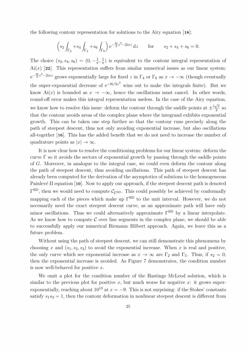
the following contour representation for solutions to the Airy equation [18]:
(s2
∫
Γ2
+s4
∫
Γ4
+s6
∫
Γ6
)e−
8i3 z
3−2ixz dz for s2 + s4 + s6 = 0.
The choice (s2, s4, s6) = (0,− 1π ,
1π ) is equivalent to the contour integral representation of
Ai(x) [22]. This representation suffers from similar numerical issues as our linear system:
e−8i3 z
3−2ixz grows exponentially large for fixed z in Γ4 or Γ6 as x→ −∞ (though eventually
the super-exponential decrease of e−8i/3z3 wins out to make the integrals finite). But we
know Ai(x) is bounded as x → −∞, hence the oscillations must cancel. In other words,
round-off error makes this integral representation useless. In the case of the Airy equation,
we know how to resolve this issue: deform the contour through the saddle points at ± i√x
2 so
that the contour avoids areas of the complex plane where the integrand exhibits exponential
growth. This can be taken one step further so that the contour runs precisely along the
path of steepest descent, thus not only avoiding exponential increase, but also oscillations
all-together [16]. This has the added benefit that we do not need to increase the number of
quadrature points as |x| → ∞.
It is now clear how to resolve the conditioning problems for our linear system: deform the
curve Γ so it avoids the sectors of exponential growth by passing through the saddle points
of G. Moreover, in analogue to the integral case, we could even deform the contour along
the path of steepest descent, thus avoiding oscillations. This path of steepest descent has
already been computed for the derivation of the asymptotics of solutions to the homogeneous
Painleve II equation [10]. Now to apply our approach, if the steepest descent path is denoted
ΓSD, then we would need to compute CΓSD . This could possibly be achieved by conformally
mapping each of the pieces which make up ΓSD to the unit interval. However, we do not
necessarily need the exact steepest descent curve, as an approximate path will have only
minor oscillations. Thus we could alternatively approximate ΓSD by a linear interpolate.
As we know how to compute C over line segments in the complex plane, we should be able
to successfully apply our numerical Riemann–Hilbert approach. Again, we leave this as a
future problem.
Without using the path of steepest descent, we can still demonstrate this phenomena by
choosing x and (s1, s2, s3) to avoid the exponential increase. When x is real and positive,
the only curve which see exponential increase as x → ∞ are Γ2 and Γ5. Thus, if s2 = 0,
then the exponential increase is avoided. As Figure 7 demonstrates, the condition number
is now well-behaved for positive x.
We omit a plot for the condition number of the Hastings–McLeod solution, which is
similar to the previous plot for positive x, but much worse for negative x: it grows super-
exponentially, reaching about 1013 at x = −9. This is not surprising: if the Stokes’ constants
satisfy s1s3 = 1, then the contour deformation in nonlinear steepest descent is different from
25

20 40 60 80 100n
10
50
20
30
15
-5 0 5 10x
100
1000
104
105
106
107
Figure 7: For (s1, s2, s3) = (1, 0,−1), the condition number of the first linear system, on the leftfor x = 0 (plain), 2.5 (dotted), 5 (dashed) and 7.5 (thick) and on the right for n = 20 (plain), 40(dotted), 60 (dashed) and 80 (thick).
the case where s1s3 6= 1, as is the asymptotic behaviour as x approaches infinity [15].
Therefore, in the limit as x becomes large, the behaviour of Painleve II has a jump as the
Stokes’ constants pass over s1s3, and the solution itself is unstable. However, if we treat
s1s3 = 1 as a special case, it may still be possible to overcome this issue. This is not
completely unlike the Airy function solution to the Airy equation for large positive x, where
perturbations of s2 will introduce exponential growth. Assuming s2 = 0 and this instability
is avoided.
7. Closing remarks
We have demonstrated that a Riemann–Hilbert formulation is not just useful as an ana-
lytical tool, but also as a numerical one, by successfully computing solutions to the homoge-
neous Painleve II equation. This could potentially lay the groundwork for the construction
of a toolbox for computing Painleve equations. Then Painleve transcendentals would indeed
be the true analogues of linear special functions such as the Airy equation: not only useful
for analytical expressions, but efficient for practical computations as well.
In Figure 8 we depict the curves Γ for the first five Painleve Riemann–Hilbert problems,
including the inhomogeneous Painleve II equation. The important characteristic to note
is that they consist of a union of curves which each can be conformally mapped to the
unit interval using Mobius transformations: rays, arcs and line segments. Thus the general
approach of Algorithm 1.3 can already be implemented for these equations. So far the
Painleve III and Painleve IV Riemann–Hilbert problems have successfully been evaluated
using RHPackage [23, 24].
Because of the numerical problems described in Section 6, this approach is currently
not practical for large x, though it is likely that using the path of steepest descent will
rectify this issue (initial numerical experiments confirm this). However, it is practical for
small x, in particular for computing initial conditions. Thus it can already be used to
26

I III
IV V
II
Figure 8: A depiction of the curves Γ associated with the Painleve I–V equations.
connect asymptotic formulæ — which are known in terms of the constants (s1, s2, s3) —
to initial conditions. A simple numerical implementation for the computation of solutions
to the homogeneous Painleve II transcendent might appear to be straightforward: use the
proposed approach for small x, use asymptotic formulæ for large |x| and use an ODE solver
to extend these two regimes to moderate x. Several issues make such an approach impractical
in general: only a few terms of the asymptotic expansion are known, requiring x to be very
large; poles on the real line prevent numerical integration; and special solutions such as
Hastings–McLeod are extremely sensitive to errors in initial conditions.
Acknowledgments : I wish to thank Folkmar Bornemann for several interesting discussions,
and for helping me to realize the importance and peculiarity of the Hastings–McLeod solu-
tion, as well as the difficulty in extending the asymptotic solution using ODE solvers. I also
thank Peter Clarkson, Toby Driscoll, Arno Kuijlaars, Thanasis Fokas, Nick Trefethen, Andy
Wathen, Andre Weideman and the anonymous referees for their valuable advice.
References
[1] Ablowitz, M.J. and Segur, H., Solitons and the inverse scattering transform, Society for
Industrial Mathematics, 2006.
27

[2] Abramowitz, M. and Stegun, I., Handbook of Mathematical Functions, National Bureau
of Standards Appl. Math. Series, #55, U.S. Govt. Printing Office, Washington,
D.C., 1970.
[3] Aksenov, S., Savageau, M.A., Jentschura, U.D., Becher, J., Soff, G. and Mohr, P.J.,
Application of the combined nonlinear-condensation transformation to problems in
statistical analysis and theoretical physics, Comp. Phys. Comm. 150 (2003), 1–20.
[4] Bateman, H., Higher Transcendental Functions, McGraw-Hill, New York, 1953.
[5] Berrut, J.-P. and Trefethen, L.N., Barycentric lagrange interpolation, SIAM Review 46
(2004), 501–517.
[6] Bornemann, F., On the numerical evaluation of Fredholm determinants, Maths Comp
79 (2010), 871–915.
[7] Boyd, J.P., Chebyshev and Fourier spectral methods, Dover Pubns, 2001.
[8] Clenshaw, C. W. and Curtis, A. R., A method for numerical integration on an
automatic computer, Numer. Math. 2 (1960), 197–205.
[9] Deift, P., Orthogonal polynomials and random matrices: a Riemann-Hilbert approach,
American Mathematical Society, 2000.
[10] Deift, P. and Zhou, X., Asymptotics for the Painleve II equation, Communications on
Pure and Applied Mathematics 48 (1995), 277.
[11] Deift, P. and Zhou, X., A steepest descent method for oscillatory Riemann-Hilbert
problems,AMS 26 (1992), 119–124.
[12] Dieng, M., Distribution Functions for Edge Eigenvalues in Orthogonal and Symplectic
Ensembles: Painleve Representations, Ph.D. Thesis, University of Davis, 2005.
[13] Dienstfrey, A., The Numerical Solution of a Riemann-Hilbert Problem Related to
Random Matrices and the Painleve V ODE, Ph.D. Thesis, Courant Institute of
Mathematical Sciences, 1998.
[14] Driscoll, T. A., Bornemann, F. and Trefethen, L. N., The chebop system for automatic
solution of differential equations, BIT 48 (2008), 701-723.
[15] Fokas, A.S., Its, A.R., Kapaev, A.A. and Novokshenov,V.Y., Painleve transcendents:
the Riemann-Hilbert approach, American Mathematical Society, 2006.
[16] Gil, A., Segura, J. and Temme, N.M., Numerical Methods for Special Functions, SIAM,
2007.
28

[17] Hastings, SP and McLeod, JB, A boundary value problem associated with the second
Painleve transcendent and the Korteweg-de Vries equation, Archive for Rational
Mechanics and Analysis 73 (1980), 31–51.
[18] Its, A.R., The Riemann-Hilbert problem and integrable systems,Notices AMS 50
(2003), 1389–1400.
[19] Masoero, D., A Simple Algorithm for Computing Stokes Multipliers, preprint, Arxiv
preprint arXiv:1007.1554, 2010.
[20] Muskhelishvili, N.I., Singular Integral Equations, Groningen: Noordhoff (based on the
second Russian edition published in 1946), 1953.
[21] Nasser, M.M.S., Numerical solution of the Riemann-Hilbert problem, Punjab
University Journal of Mathematics 40 (2008), 9–29.
[22] Olver, F.W.J., Asymptotics and Special Functions, Academic Press, New York, 1974.
[23] Olver, S., RHPackage, http://www.comlab.ox.ac.uk/people/
Sheehan.Olver/projects/RHPackage.html
[24] Olver, S., A general framework for solving Riemann–Hilbert problems numerically,
preprint, NA-10/05, Maths Institute, Oxford University.
[25] Olver, S., Computing the Hilbert transform and its inverse, Maths Comp, to appear.
[26] Prahofer, M. and Spohn, H., Exact scaling functions for one-dimensional stationary
KPZ growth, http://www-m5.ma.tum.de/KPZ/
[27] Prahofer, M. and Spohn, H., Exact scaling functions for one-dimensional stationary
KPZ growth, J. Stat. Phys. 115 (2004), 255–279.
[28] Tracy, C.A. and Widom, H., Level-spacing distributions and the Airy kernel, Comm.
Math. Phys. 159 (1994), 151–174.
[29] Wegert, E., An iterative method for solving nonlinear Riemann-Hilbert problems, J.
Comp. Appl. Maths 29 (1990), 327.
[30] Wegmann, R., Discrete Riemann-Hilbert problems, interpolation of simply closed
curves, and numerical conformal mapping, J. Comp. Appl. Maths 23 (1988),
323–352.
[31] Wegmann, R., An iterative method for the conformal mapping of doubly connected
regions,J. Comp. Appl. Maths 14 (1986), 79–98.
29