numerical solution of the time-domain...

NUMERICAL SOLUTION OF THE TIME-DOMAIN

MAXWELL EQUATIONS USING HIGH-ACCURACY

FINITE-DIFFERENCE METHODS∗

H. M. JURGENS† AND D. W. ZINGG†

SIAM J. SCI. COMPUT. c© 2000 Society for Industrial and Applied MathematicsVol. 22, No. 5, pp. 1675–1696

Abstract. High-accuracy finite-difference schemes are used to solve the two-dimensional time-domain Maxwell equations for electromagnetic wave propagation and scattering. The high-accuracyschemes consist of a seven-point spatial operator coupled with a six-stage Runge–Kutta time-marchingmethod. Two methods are studied, one of which produces the maximum order of accuracy and oneof which is optimized for propagation distances smaller than roughly 300 wavelengths. Boundaryconditions are presented which preserve the accuracy of these schemes when modeling interfacesbetween different materials. Numerical experiments are performed which demonstrate the utility ofthe high-accuracy schemes in modeling waves incident on dielectric and perfect-conducting scatterersusing Cartesian and curvilinear grids. The high-accuracy schemes are shown to be substantially moreefficient, in both computing time and memory, than a second-order and a fourth-order method. Theoptimized scheme can lead to a reduction in error relative to the maximum-order scheme, with noadditional expense, especially when the number of wavelengths of travel is large.

Key words. computational electromagnetics, finite-difference schemes, wave propagation, phaseerror, Maxwell’s equations

AMS subject classifications. 78M20, 65M06

PII. S1064827598334666

1. Introduction. Numerical simulation of the propagation and scattering ofelectromagnetic waves has a wide range of applications in science and engineering,including antennas, microwave circuits, high-speed digital interconnects, all-opticaldevices, and many more [23]. The appropriate numerical algorithm for such simula-tions is dependent on the nature of the system being modeled. For geometries of lowelectrical size, i.e., spanning at most a few wavelengths, the method of moments is anefficient technique. However, scaling arguments presented by Petropoulos [18] showthat this approach quickly becomes impractical as the electrical size increases. Ge-ometries of moderate electrical size can be handled effectively using several availablenumerical methods for solving the Maxwell equations in the time domain. For suchsimulations, the geometric flexibility of the finite-element method can compensate forits relative inefficiency for hyperbolic equations. More efficient methods, which areeffective for propagation distances on the order of 10 or 20 wavelengths, include thefinite-difference methods of Yee [28] and Shang [20] and the finite-volume method ofMohammadian, Shankar, and Hall [16]. However, for propagation distances greaterthan 20 wavelengths, these methods, which are second-order accurate, typically re-quire excessive grid densities with correspondingly large computational requirements.

The limitations of second-order methods in simulating wave phenomena have ledto the development and application of higher-order and optimized finite-differencemethods in several fields, including acoustics [13, 24] and seismology [10], as wellas electromagnetics [12, 21, 25, 27, 29, 31, 34]. Higher-order methods offer increasedaccuracy for a given node density at the expense of increased cost per node. Optimized

∗Received by the editors February 27, 1998; accepted for publication (in revised form) June 14,2000; published electronically December 20, 2000.

http://www.siam.org/journals/sisc/22-5/33466.html†Institute for Aerospace Studies, University of Toronto, 4925 Dufferin Street, Downsview, ON,

Canada M3H 5T6 ([email protected], [email protected]).

1675

1676 H. M. JURGENS AND D. W. ZINGG

schemes sacrifice the order of accuracy in return for low error over an increased rangeof wavenumbers. Fourier analysis provides a simple means of analyzing the phase andamplitude errors of finite-difference methods [14, 26, 31, 34]. Several high-order andoptimized schemes were compared by Zingg [30] using this approach. Zingg showedthat one of the optimized compact schemes developed by Haras and Ta’asan [6] iscapable of accurate simulations involving 200 wavelengths of travel with less than4 grid points per wavelength. This scheme requires the solution of a pentadiagonalsystem of equations in each coordinate direction. The optimized noncompact schemesof Lockard, Brentner, and Atkins [15] and Zingg, Lomax, and Jurgens [34, 35] requireless than 10 grid points per wavelength for 200 wavelengths of travel with a muchlower cost per node. Numerical experiments are required to determine the relativeefficiencies of these methods in a practical context.

In order to avoid the use of a very small time step, the accuracy of the time-marching method should be comparable to that of the spatial operator. For simulatingwave phenomena, Runge–Kutta and Adams–Bashforth methods are natural candi-dates, with the former generally preferred due to their low memory requirements. Forlinear ordinary differential equations with constant coefficients, Runge–Kutta meth-ods of up to fourth order require only two memory locations per dependent variable[31]. Five- and six-stage methods with the same memory requirement have beenproposed by Haras and Ta’asan [6] and Zingg, Lomax, and Jurgens [34, 35].

The need for stable and accurate numerical boundary schemes presents a ma-jor obstacle in the application of high-order finite-difference methods. Since longpropagation distances are generally associated with multiple interactions with me-dia interfaces, the numerical boundary schemes can have a significant impact on theoverall accuracy of a simulation, and hence on the relative accuracy of various meth-ods. Progress in the development of numerical boundary schemes was reported in [4,17, 33]. Another important consideration in the application of high-order methodsis the choice of gridding strategy. Uniform Cartesian grids were used, for example,by Taflove and co-workers [23], while body-fitted curvilinear grids were favored byShankar, Mohammadian, and Hall [22] and others. The Cartesian approach producestwo significant advantages in the interior of the domain. Virtually all numerical meth-ods are most accurate on a uniform grid. In addition, the need to deal with the metricsof a curvilinear coordinate transformation leads to a substantial penalty in terms ofboth speed and memory. On the other hand, it is extremely difficult to develop sta-ble and accurate boundary treatments for higher-order methods on Cartesian grids.Furthermore, some geometries, such as a curved surface with a thin coating, are notwell suited to Cartesian grids. Clearly, the choice of a gridding strategy is problemdependent.

A further issue in the development of numerical methods for the time-domainMaxwell equations is the need to truncate the domain, which inevitably leads to spu-rious reflections. Boundary conditions based on locally one-dimensional characteristicsplitting generally produce excessive reflection. Thus, development of nonreflectingboundary conditions for hyperbolic problems has been an active area of research formany years. Important contributions have been made by Engquist and Majda [5],Bayliss and Turkel [2], Berenger [3], and Petropoulos, Zhao, and Cangellaris [19].

This paper presents the implementation and validation of the high-order andoptimized finite-difference methods presented in [34, 35] for the solution of the time-domain Maxwell equations. The objective is to demonstrate the efficiency of thesemethods on nontrivial sample problems. The methods combine a noncompact spatial

HIGH-ACCURACY FINITE-DIFFERENCE SCHEMES 1677

operator with a seven-point stencil and a low-storage six-stage time-marching method.Two methods are studied, one of which produces the maximum order of accuracy andone of which is optimized for propagation distances less than roughly 300 wavelengths.In the next section, the Maxwell equations are presented in generalized curvilinearcoordinates. The two finite-difference methods, including both spatial and temporaloperators, are then presented. This is followed by a description of the treatment ofinterfaces and boundaries, including dielectric interfaces, perfect conductors, and do-main boundaries. The two methods are applied to a number of test problems involvingthe propagation and scattering of electromagnetic waves. In order to demonstrate theefficiency of the present methods, the computational requirements are compared withtwo other methods, one fourth order in space, the other second order.

2. Governing equations. In two dimensions, Maxwell’s equations decoupleinto two sets, the transverse magnetic (TM) and the transverse electric (TE) equa-tions. Without any loss of physics, we consider only the TM set. We restrict ourattention to linear, isotropic, perfect dielectric materials with constant properties, nocharge density, and no current sources. Under these conditions, the TM equationscan be written in the following form:

∂Q

∂t+ A

∂Q

∂x+ B

∂Q

∂y= 0.(2.1)

The vector of unknowns is given by

Q =

Dz

Bx

By

,(2.2)

where Dz is the z component of the electric flux density, Bx and By are the x and ycomponents of the magnetic flux density, and the two matrices are

A =

0 0 −1

µ

0 0 0

−1

ε0 0

, B =

01

µ0

1

ε0 0

0 0 0

;(2.3)

µ is the magnetic permeability and ε is the electric permittivity. The constitutiverelations are D = εE and B = µH, where E is the electric field intensity and H isthe magnetic field intensity. In our tests, we assume a nondimensional form of theequations where, in free space, ε = µ = 1. Note that the divergence relations are notexplicitly enforced. However, numerous tests with the numerical methods studied inthis paper show that the divergence of the magnetic field remains of the order of thetruncation error for all time.

When numerically modeling electromagnetic fields, it is often the case that thegeometry of the problem lends itself to a more generalized coordinate system thanCartesian. A method that allows the independent variables of the partial differentialequations to be transformed into a uniformly spaced computational domain was givenin [1]. The two-dimensional TM form of Maxwell’s curl equations can be expressedin a generalized coordinate system using the following transformation:

ξ = ξ(x, y), η = η(x, y).(2.4)


This allows the Cartesian coordinates to be transformed into curvilinear coordinatesin such a way that a curvilinear grid will map to a uniform and square computationalspace with ∆ξ = ∆η = 1. The mapping is usually defined by assigning integercurvilinear coordinate values to each node in the grid and calculating the metricsof the transformation numerically. The transformed equations can be written in thefollowing form:

∂Q

∂t+ A

∂Q

∂ξ+ B

∂Q

∂η= 0,(2.5)

where the two matrices are

A =

01

µ

∂ξ

∂y−

1

µ

∂ξ

∂x

1

ε

∂ξ

∂y0 0

−1

ε

∂ξ

∂x0 0

, B =

01

µ

∂η

∂y−

1

µ

∂η

∂x

1

ε

∂η

∂y0 0

−1

ε

∂η

∂x0 0

.(2.6)

Extension to spatially variable material properties requires the use of a strong-conservation-law form of the equations, as discussed in [11].

3. Numerical method. Our aim is to solve for the total electric and magneticfield components by approximating Maxwell’s equations using finite-difference meth-ods. The finite-difference schemes used consist of a seven-point spatial operator inconjunction with an explicit six-stage time-marching method. These high-accuracymethods were originally presented by Zingg, Lomax, and Jurgens [35], and an ex-tensive description of the methods, including an error and stability analysis, can befound in [34].

The spatial operator is made up of two parts, an antisymmetric or central-difference operator,

(δaxu)j =1

∆x[a1(uj+1 − uj−1) + a2(uj+2 − uj−2) + a3(uj+3 − uj−3)],(3.1)

and a symmetric operator,

(δsxu)j =1

∆x[d0uj + d1(uj+1 + uj−1) + d2(uj+2 + uj−2) + d3(uj+3 + uj−3)].(3.2)

The operator described by (3.1) has a maximum formal order which varies as ∆x6

when a1 = 34 , a2 = − 3

20 , and a3 = 160 . The operator described by (3.2) has a maximum

formal order which varies as ∆x5 when d1 = − 34d0, d2 = 3

10d0, and d3 = − 120d0. The

symmetric operator is used to add a small amount of numerical dissipation to thescheme. We use a value of d0 = 1

10 . A characteristic splitting is used when theoperator is applied to a hyperbolic system of equations. For example, in order toapproximate the term A∂Q

∂x , the scheme is applied as follows:

A

(

∂Q

∂x

)

j

= A(δaxQ)j + |A|(δsxQ)j(3.3)

at any interior node j. Note that |A| = X|Λ|X−1, where X is the matrix of righteigenvectors of A, and Λ is the matrix of eigenvalues of A. The method is applied ina similar way in order to approximate the y-derivatives of the field values.


The time-marching method, when applied to the ordinary differential equationdudt = f(u, t), can be written as

u(1)n+α1

= un + hα1fn,

u(2)n+α2

= un + hα2f(1)n+α1

,

u(3)n+α3

= un + hα3f(2)n+α2

,(3.4)

u(4)n+α4

= un + hα4f(3)n+α3

,

u(5)n+α5

= un + hα5f(4)n+α4

,

un+1 = un + hf(5)n+α5

,

where h = ∆t is the time step, tn = nh, un = u(tn), and f(k)n+α = f(u

(k)n+α, tn + αh).

Setting α5 = 12 gives a method that is second-order accurate. Additionally setting

α4 = 13 , α3 = 1

4 , α2 = 15 , and α1 = 1

6 gives the method with the highest formal orderfor linear homogeneous ordinary differential equations, which is sixth-order accurate.For inhomogeneous and nonlinear ordinary differential equations, it is second-orderaccurate. Two memory locations are required per dependent variable. The stabilityregion for this method was shown in [34].

The above operators contain coefficients that can be determined in a numberof ways. We have already described the operators in which the coefficients are de-termined by maximizing the formal order (referred to as the maximum-order (MO)operator). Zingg, Lomax, and Jurgens [34, 35] presented an additional method, inwhich the coefficients are determined by specifying that the phase and amplitude er-rors of the operators are minimized for waves which are resolved by the computationalgrid with at least 10 points per wavelength (referred to as the optimized operator orO10). The coefficients for this optimized scheme can be found in the appendix.

These schemes have a number of useful properties. First, the amplitude error isless than the phase error for all wavenumbers [34]. Hence any wavenumber compo-nents that are excessively damped also have excessive phase error. Second, the time-marching method produces significantly smaller errors than the spatial discretization.Hence the phase and amplitude errors are virtually independent of the Courant num-ber (for Courant numbers less than unity). This contrasts with some other schemesthat are accurate only within a narrow range of Courant numbers. Similarly, thepresent schemes do not require that the direction of wave propagation be alignedwith the grid. The errors are largest for propagation angles of zero and 90 degrees.Hence the one-dimensional analysis given in [34] gives an upper bound on the error.

4. Interface and boundary treatment. In order to simulate the scatteringof electromagnetic waves off of materials which have differing dielectric properties,each region is modeled as a distinct numerical domain. These domains are thencoupled using the appropriate physical boundary conditions. This procedure allowsthe grids for each region to be generated independently, which is useful since theresolution of the grid is dependent on the material properties of the domain. Threeseparate boundary types are considered, an interface between two dielectric regions,the boundary between a dielectric and a perfect conductor, and the far-field boundarywhich is located at the outer region of the domain. At the interface between twodielectric media and at the surface of a perfect conductor, a locally one-dimensionalcharacteristic formulation of the governing equations is used [8]. Using this approach,


characteristic variables can be found that represent incoming and outgoing wavesalong lines normal to the interface. For example, if we consider a boundary thatlies at the right side of the domain on a line of constant x, the incoming waves areassociated with A− and the outgoing waves with A+, where

A± =A ± |A|

2(4.1)

and |A| is defined after (3.3). Similar expressions can be found for boundaries thatlie on lines of constant y and for boundaries in curvilinear coordinates. For thecurvilinear case, the incoming and outgoing waves will be associated with A± andB±. When calculating spatial derivatives near boundaries and interfaces, flux-vectorsplitting is used. Regular fifth-order one-sided and upwind-biased schemes are usedfor the outgoing waves, while the following numerical boundary scheme (NBS) is usedfor the incoming waves:

(δxu)1 =1

60∆x[−3u0 − 119u1 + 255u2 − 240u3 + 155u4 − 57u5 + 9u6],

(4.2)(δxu)2 =

1

60∆x[9u0 − 66u1 + 70u2 − 60u3 + 75u4 − 34u5 + 6u6].

The above NBS is a modified version of the one presented by Zingg, Lomax, andJurgens [34, 35], which was found to be unstable on some curvilinear grids.

4.1. Dielectric interfaces. On the interface between two dielectrics the follow-ing conditions must hold:

E(1)t = E

(2)t ,(4.3)

H(1)t = H

(2)t ,(4.4)

D(1)n = D(2)

n ,(4.5)

B(1)n = B(2)

n .(4.6)

The superscripts refer to the field values in materials (1) and (2). Note that theserelations assume that there is no surface current flowing along the interface and thatthere is no surface charge density present at the interface. In the TM case, the electricintensity and electric flux density vectors point out of the x-y plane, and thus (4.5)holds automatically and (4.3) simplifies to

E(1)z = E(2)

z .(4.7)

Consider a body-fitted grid which ensures that the interface between differentmaterials will lie on a ξ = constant curve. The grid is constrained to be orthogonalnear the body, thus η = constant curves are normal to the interface. In this example,we assume that the positive ξ direction points from region (1) to region (2). Figure 1shows an example of such a body-fitted coordinate system. We can generalize thisexample to different cases in curvilinear coordinates and to Cartesian coordinatesquite easily. There are six unknown values which need to be stored on the interface:

D(1)z , D

(2)z , B

(1)x , B

(2)x , B

(1)y , and B

(2)y . The fields are extrapolated to the interface

using a sixth-order method (see the appendix). The characteristic variables are thencalculated from

w(1)+ = Z(1)D(1)

z + B(1)t(4.8)


Fig. 1. Example of a body-fitted grid showing the characteristic variables associated with the

outgoing waves.

and

w(2)− = Z(2)D(2)

z −B(2)t ,(4.9)

where Z = (µ/ε)1/2 is the intrinsic impedance of the medium. Note that

Bt =

∂ξ

∂yBx −

∂ξ

∂xBy

[

(

∂ξ

∂x

)2

+

(

∂ξ

∂y

)2]1/2

(4.10)

is the component of B tangent to a ξ = constant curve, and

Bn =

∂ξ

∂xBx +

∂ξ

∂yBy

[

(

∂ξ

∂x

)2

+

(

∂ξ

∂y

)2]1/2

(4.11)

is the component of B normal to a ξ = constant curve. This gives two equations for

the unknown values D(1)z , D

(2)z , B

(1)t , and B

(2)t . Note that the quantities extrapo-

lated depend on the orientation of the local (ξ, η) coordinate system at the interface.Combining these with the jump conditions, we obtain

D(1)z =

w(1)+ +

µ(1)

µ(2)w

(2)−

Z(1)

(

1 +Z(1)

Z(2)

),(4.12)

D(2)z =

ε(2)

ε(1)D(1)

z ,(4.13)


B(1)t =

Z(1)w(1)+ − µ(1)c(2)w

(2)−

Z(1) + Z(2),(4.14)

B(2)t =

µ(2)

µ(1)B

(1)t .(4.15)

The variable c = (εµ)−1/2 is the propagation speed. The normal component of themagnetic flux density is single valued on the interface, as shown by (4.6), and isdetermined by averaging the two values obtained by extrapolation. The values of Bx

and By are determined from Bn and Bt using (4.10) and (4.11).The above interface treatment was closely examined in [32]. The error introduced

at interfaces is of the same order of magnitude as that introduced in the interiorusing the high-accuracy schemes. Both the interior discretization and the interfacetreatment, including the NBS (4.2), contribute to the overall error, with the relativecontribution depending on the distance between interfaces.

4.2. Perfect conductors. At the interface between a dielectric material and aperfect conductor, the physical boundary conditions given in the above section mustbe modified. If, for example, region (2) is a perfect conductor—that is, having aninfinite conductivity—then all the field values inside the region must be zero. Usingthis fact, and the four relations given in the above section, one obtains the followingboundary conditions at the surface of a perfect conductor:

Et = 0,(4.16)

Ht = Js,(4.17)

Dn = 0,(4.18)

Bn = 0.(4.19)

In general, there will always be a finite current density, Js, on the surface of a perfectconductor, but we have assumed a zero surface charge density. For the TM case,the third condition is automatically satisfied since the electric flux density points outof the plane, and the first condition sets its magnitude to zero, i.e., Dz = 0. Thetangential component of the magnetic flux density, and thus the surface current, isfound by extrapolating the fields to the surface and then calculating the outgoingcharacteristic variable. For example, if the surface of the perfect conductor lies alonga grid line of constant ξ, with ξ increasing as the boundary is approached, then w+

is determined from (4.8). Since Dz = 0, (4.8) gives

Bt = w+,(4.20)

where Bt is defined by (4.10). The Cartesian components of the magnetic flux densityare determined using this value and the fact that Bn = 0.

4.3. Far-field boundaries. To model the problem of waves moving out intofree space, the numerical domain must be artificially truncated. There is a consid-erable body of literature on the subject of far-field boundary conditions which triesto minimize the spurious reflection introduced when a disturbance propagates out ofthe numerical domain [2, 3, 5, 19, 23, 24]. There are many papers, such as [9], thatdiscuss the merits of different types of far-field conditions.

We implement a modified version of the radiating boundary condition introducedby Bayliss and Turkel [2], which was found to be the best method of those tested by


Hixon, Shih, and Mankbadi [9]. This method truncates the domain by using a far-field radiation condition which only allows disturbances to propagate in the outwarddirection. The condition is applied by enforcing the following partial differentialequation on the boundary region of the domain:

(

1

c

∂

∂t+

∂

∂r+

a

2r

)

Dz

Bx

By

= 0.(4.21)

When a = 1 the operator given in [2] is recovered, which is O(r−5/2). Using theoperator with this value of a results in the numerical schemes becoming unstable forsome curvilinear grids. We use a value of a = 3, which results in a stable and accuratemethod. The numerical domain is split into two regions, one of which contains thetotal electromagnetic field and one of which contains only the scattered field (see,for example, [23]). We store the scattered field on ghost-points which lie outside thedomain, and the total field at all other nodes. To approximate the spatial derivativesin Maxwell’s equations where the computational stencil will overlap the ghost-pointregion, the incident field is added to the scattered field at the necessary nodes inthis region. When calculating the spatial derivatives for the radiation condition, theincident field is subtracted from the total field at the necessary nodes in the interiordomain.

5. Results and discussion.

5.1. Dielectric square. We first simulate the scattering of a pulsed plane waveoff of a dielectric square. Figure 2 shows an example grid as well as the geometryof the problem. The domain is square, with x and y ranging from 0 to 1, and thedielectric is located in the center of this region, at 0.4 ≤ x ≤ 0.6, 0.4 ≤ y ≤ 0.6.The permittivity of the dielectric is four times that of the free space region. Thewavespeed in free space is normalized to one, resulting in a wavespeed of one-half inthe dielectric. The domain is discretized using a Cartesian grid, in which ∆x = ∆y,and the grid density in the interior of the dielectric is twice that of free space. Resultsare obtained for a Gaussian pulse incident upon the dielectric square at an angle of45◦. The incident electric field is given by

Ez(x, y, t) = exp

[

−1

2σ2

(

x cosπ

4+ y sin

π

4+

1

2− t

)2]

(5.1)

with σ = 0.03. For all test cases, the time step is chosen in order to give a Courantnumber of unity in free space. This results in a value of ∆t equal to the ∆x value of thefree space domain. As a result of both the wave speed and the grid spacing inside thedielectric being one half the values found outside the dielectric, the Courant numberwill also have a value of unity inside the dielectric. This ensures that the spatialresolution inside the dielectric is matched with that found in free space, since thewidth of the pulse will narrow as it slows down. Because of this, the errors will notbe as localized to the interior of the dielectric as they were in the tests performedin section 5.1 of [11], where the grid resolution was kept constant over the entiredomain. The better grid resolution inside the dielectric also allows for an accuratesimulation of a narrower pulse. Note, however, that the accuracy of the high-accuracyfinite-difference schemes is equally good at Courant numbers less than unity. Spuriousreflections are not an issue for this case because the incident field is imposed along


Fig. 2. Example grid showing pulsed plane wave with Gaussian cross-section incident at 45◦

on a dielectric square.

the entire outer boundary, and the simulation is not run long enough for the reflectedpulse to reach the outer boundary.

For this simulation the interfaces between the different materials lie along linesin the Cartesian grid. The jump conditions discussed in section 4.1 can be used toobtain the field values along grid lines that cross the interfaces. In order to obtainthe field unknowns along the interface at nodes inside the dielectric, which do nothave a corresponding node outside the dielectric, interpolation and extrapolation ofvalues from neighboring interface nodes are used. The interpolation and extrapolationschemes can be found in the appendix. Note that the extrapolation scheme and thenoncentered interpolation schemes are used for the nodes near the corners of thedielectric. The corners must also be treated as special cases. It is only necessary tostore the field values at the corner nodes for the free space part of the domain sincethe values in the interior of the dielectric are never used during the simulation. Thesevalues are obtained by taking the average value of the results of interpolating the fieldvalues along the x and y grid lines which intersect the corner node. Again, the relevantinerpolation schemes can be found in the appendix. Note that the presence of the


Fig. 3. Contour plots of electric field intensity and errors in electric field intensity. (a) Refer-

ence solution, (b) MO error using 11,200 nodes, (c) C4 error using 11,200 nodes, and (d) C2 error

using 44,800 nodes.

singularity in the neighborhood of the corners introduces a low-order error locally.The finite-difference scheme can be modified locally to account for the singularity,but our results will show that the high-accuracy methods produce significant errorreduction without implementing such a strategy.

In addition to the MO and O10 schemes described here, results are presented forsecond-order centered differences in space combined with fourth-order Runge–Kuttatime marching (C2) and fourth-order centered differences in space combined withfourth-order Runge–Kutta time marching (C4).

Contour plots of the absolute value of the error in the electric field intensity att = 1.4 are shown for three different cases in Figure 3. Figure 3(a) shows the electricfield intensity for a reference solution calculated using the MO scheme on a grid with179,200 nodes. The error obtained using the MO scheme on a grid with 11,200 nodesis shown in Figure 3(b). Note that the contour levels grow exponentially, and the erroris extremely small. Plots of the errors obtained using method C4 on the grid with


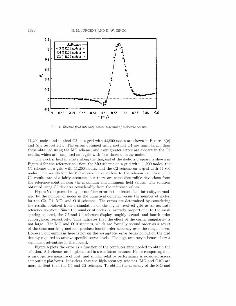
Fig. 4. Electric field intensity across diagonal of dielectric square.

11,200 nodes and method C2 on a grid with 44,800 nodes are shown in Figures 3(c)and (d), respectively. The errors obtained using method C4 are much larger thanthose obtained using the MO scheme, and even greater errors are evident in the C2results, which are computed on a grid with four times as many nodes.

The electric field intensity along the diagonal of the dielectric square is shown inFigure 4 for the reference solution, the MO scheme on a grid with 11,200 nodes, theC4 scheme on a grid with 11,200 nodes, and the C2 scheme on a grid with 44,800nodes. The results for the MO scheme lie very close to the reference solution. TheC4 results are also fairly accurate, but there are some discernible deviations fromthe reference solution near the maximum and minimum field values. The solutionobtained using C2 deviates considerably from the reference values.

Figure 5 compares the L2 norm of the error in the electric field intensity, normal-ized by the number of nodes in the numerical domain, versus the number of nodes,for the C2, C4, MO, and O10 schemes. The errors are determined by consideringthe results obtained from a simulation on the highly resolved grid as an accuratereference solution. Since the number of nodes is inversely proportional to the meshspacing squared, the C2 and C4 schemes display roughly second- and fourth-orderconvergence, respectively. This indicates that the effect of the corner singularity isnot large. The MO and O10 schemes, which are formally second order as a resultof the time-marching method, produce fourth-order accuracy over the range shown.However, our emphasis here is not on the asymptotic error behavior but on the griddensity required to achieve specified error levels. The high-accuracy schemes show asignificant advantage in this regard.

Figure 6 plots the error as a function of the computer time needed to obtain thesolution. All schemes are implemented in a consistent manner. Hence computing timeis an objective measure of cost, and similar relative performance is expected acrosscomputing platforms. It is clear that the high-accuracy schemes (MO and O10) aremore efficient than the C4 and C2 schemes. To obtain the accuracy of the MO and


Fig. 5. L2 norm of the error in the electric field intensity for the dielectric square case, as a

function of the number of nodes in the grid.

Fig. 6. L2 norm of the error in the electric field intensity for the dielectric square case, as a

function of the CPU cycles necessary to complete simulation.

O10 methods on a grid with 11,200 nodes, the C4 scheme needs to be run on a gridwith 2.5 times as many grid nodes, requiring twice as much CPU time. The resultsobtained using C2 on a grid with 16 times as many nodes gives an error which isabout 3.5 times as large as that obtained by the MO scheme, taking about 25 timeslonger to run. Even though the high-accuracy schemes take longer to run per gridnode per time step, this is easily offset by the fact that smaller errors can be obtainedby using a grid with far fewer nodes, and, as a result, a larger time step. The savingsin memory is a direct result of using a grid with fewer nodes. The savings in bothtime and memory will be even more evident in three dimensions.

For the above cases the optimized method (O10) gives the same results as theMO scheme. This is primarily due to the nature of the Gaussian pulse, which hassignificant low wavenumber content. The majority of the Fourier components of thepulse have wavenumbers that give a value of κ∆x < 0.35 on the grid with 11,200nodes. These are resolved more accurately by the MO scheme.


Fig. 7. Example grid showing pulsed plane wave with Gaussian cross-section incident on a

perfectly conducting cylinder.

5.2. Perfectly conducting cylinder. We now consider an example using acurvilinear grid which consists of a waveform incident on a perfectly conducting cylin-der. Figure 7 shows the geometry of the problem. The cylinder has a radius of unity,and the outer limit of the numerical domain is at r = 5. The speed at which a wavetravels in free space is again normalized to unity. The waveform enters the domainfrom the left. The simulations described in section 5.2 of [12] are improved by modi-fying the grids so they are made up of three distinct zones. These grids, an exampleof which is shown in Figure 7, limit the widening of individual cells as one moves awayfrom the scatterer, which allows the modeling of narrower pulses. This is a result ofdoubling the resolution of the grid, in the θ direction, whenever the value of r is dou-bled. This ensures that the waves are evenly resolved over the entire computationaldomain. The zones in the domain are allowed to overlap slightly in order to avoidthe use of boundary operators where they interface. Interpolation must be used inorder to obtain the field values at nodes that do not have corresponding nodes in thezone being overlapped. The interpolation schemes are described in the appendix. Thegrids are generated in order to obtain cells that have an aspect ratio close to 1 nearthe perfect conductor. When the aspect ratio deviates too much from this value, it isdifficult to find boundary schemes that are stable and accurate for the high-accuracymethods. For all the tests, the time step is chosen so that the Courant number fallsin the range 0.5 to 1.0. The grid metrics are calculated numerically using the sameantisymmetric operator used in the calculation of the spatial derivatives of the elec-tromagnetic fields. It should be emphasized that such a grid, i.e., one that produces asmall range of Courant numbers, is not required in order to demonstrate the efficiencyof the high-accuracy schemes, as shown in [12]. We have generated the grid in thismanner simply to show that it can easily be done and to avoid a simulation in whichthe numerical errors are introduced primarily in one region of the grid.

5.2.1. Gaussian incident pulse. Consider a pulsed plane wave with a Gaus-sian cross-section incident on the cylinder. The incident electric field intensity is givenby


Fig. 8. Contour plots of electric field intensity and errors in electric field intensity. (a) Ref-

erence solution, (b) MO error using 5,400 nodes, (c) C4 error using 5,400 nodes, and (d) C2 error

using 21,600 nodes.

Ez(x, y, t) = exp

[

−1

2σ2

(

x +15

2− t

)2]

(5.2)

with σ = 0.3, and the simulation is run until t = 8.5. Figure 8(a) shows a contourplot of the electric field intensity for a reference solution calculated using the MOscheme on a grid with 345,600 nodes. The absolute value of the error obtained usingthe MO scheme on a grid with 5,400 nodes is shown in Figure 8(b). Even though thisgrid is fairly coarse, the errors are seen to be very small. Plots of the errors obtainedusing method C4 on the grid with 5,400 nodes and method C2 on a grid with 21,600nodes are shown in Figures 8(c) and (d), respectively. Both of these solutions showsignificant deviations from the reference solution.

The electric field intensity along the x-axis, behind the perfect conductor, isshown in Figure 9. In this region, the solution is not visible in Figure 8(a) and isvery sensitive to numerical errors. The reference solution, the results from the MO


Fig. 9. Electric field intensity along a radial line behind the perfectly conducting cylinder for

an incident pulse with a Gaussian cross-section.

Fig. 10. L2 norm of the error in the electric field intensity as a function of the number of

nodes in the grid for a pulsed plane wave incident on the perfectly conducting cylinder.

scheme on a grid having 21,600 nodes, the results from the C4 scheme on a grid with21,600 nodes, and the results from the C2 scheme on a grid with 86,400 nodes are allshown. The solution obtained using the MO scheme is very accurate. Using the samegrid, the C4 method produces a solution that deviates significantly from the referencesolution. The solution obtained by using C2 on a grid with four times as many nodesis not adequate for engineering purposes.

Figure 10 shows the normalized L2 norm of the errors in the electric field intensityas a function of the number of nodes in the grid, and Figure 11 shows the error as afunction of the CPU usage. The error value for each test is calculated using a reference



CPU cycles it takes to complete the simulation for a pulsed plane wave incident on the perfectly

conducting cylinder.

solution obtained using the MO scheme on a highly resolved grid. The trends shownin these figures are very similar to those obtained for the dielectric square case. Toattain the same error level as the MO scheme used on a grid with 21,600 nodes, theC4 scheme must use about 3.25 times as many nodes and takes about 3.4 times aslong to complete the simulation. Even when using a grid with 345,600 nodes, theC2 method does not produce a solution that can compare with those computed bythe high-accuracy methods on a grid with 21,600 nodes. The O10 scheme is seen toproduce slightly better results than the MO scheme when using the same grid. Forexample, on the grid with 21,600 nodes, the O10 scheme results in an error that is61% of that obtained using the MO scheme, with no additional CPU expense.

5.2.2. Cosine incident wave. In this section, simulations of a cosine planewave incident on the perfectly conducting cylinder are presented. The existence ofan analytical solution for a plane harmonic electromagnetic wave incident upon aperfectly conducting circular cylinder is well known and can be found in, for example,[7]. The incident electric field intensity is given by

Ez(x, y, t) = cosκ(x− t)(5.3)

with κ = 2π. A shaded contour plot of the analytical solution for the total electricfield intensity is shown in Figure 12.

Figure 13 compares the errors as a function of the number of nodes in the grids.Figure 14 plots these errors as a function of the CPU time needed to complete the sim-ulations. These plots again show the superior efficiency of the high-accuracy methods.The second-order method produces significant errors for all three of the grids. Thefourth-order method needs to use the most resolved grid to generate a solution withacceptable accuracy, which can be produced by the high-accuracy methods on a gridwith four times fewer nodes. Figure 15 shows the electric field intensity along a radialline directly behind the scatterer for the analytical, fourth-order, and MO solutions.The numerical solutions were obtained on a grid with 21,600 nodes. The solution ob-


Fig. 12. Electric field intensity for cosine wave, with κ = 2π, incident on a perfectly conducting

cylinder.


nodes in the grid for a cosine wave, with κ = 2π, incident on the perfectly conducting cylinder.

tained using the MO method is considerably more accurate than that obtained usingthe fourth-order method.

The optimized scheme does not show significant improvement over the maximum-order scheme in the above tests because of the relatively short distance of travel for thewaves being considered. To test longer distances of travel (in terms of wavelength) ahighly resolved grid with 345,600 nodes is used, and incident waves with much higherwavenumbers are modeled. With κ = 8π, the wave is resolved with 10 to 20 PPW andtravels 32 wavelengths during the simulation. For this case, the optimized methodproduces an error that is about 40% of that produced by the MO scheme. With


Fig. 14. L2 norm of the error in the electric field intensity as a function of the CPU time

necessary to complete the simulation for a cosine wave, with κ = 2π, incident on the perfectly

conducting cylinder.

Fig. 15. Electric field intensity along a radial line behind the perfectly conducting cylinder for

an incident cosine wave with κ = 2π.

κ = 10π, the resolution is 8 to 16 PPW, and the distance of travel is 40 wavelengths.For this wavenumber, the optimized method produces an error that is about 25% ofthat produced by the maximum-order scheme. This shows that the benefits of theoptimized scheme increase as the number of wavelengths traveled between reflectionsincreases.

6. Conclusions. Two high-accuracy finite-difference schemes have been used tosolve the two-dimensional time-domain Maxwell equations to simulate electromagneticwave propagation and scattering. The schemes have successfully modeled perfectly


conducting and dielectric scatterers on Cartesian and curvilinear grids. The high-accuracy methods have been shown to be more efficient than classical second-orderand fourth-order methods in terms of computing time and memory. The optimizedscheme can produce some error reduction relative to the maximum-order scheme withno additional expense, especially when the number of wavelengths of travel is large.Overall, the results demonstrate that these methods are an efficient option for simu-lating the propagation and scattering of high-frequency electromagnetic waves.

Appendix. The following are the coefficients of the optimized scheme:

a1 = 0.759961, a2 = −0.158122, a3 = 0.0187609,

d0 = 0.1, d1 = −0.0763846, d2 = 0.0322896, d3 = −0.005905,

α1 = 0.168850, α2 = 0.197348, α3 = 0.250038, α4 = 0.333306, α5 = 0.5.

The following are the extrapolation and interpolation schemes used along interfaces:

uj = 6uj+1 − 15uj+2 + 20uj+3 − 15uj+4 + 6uj+5 − uj+6,

uj+1/2 = (3uj−2 − 25uj−1 + 150uj + 150uj+1 − 25uj+2 + 3uj+3)/256,

uj+1/2 = (−7uj−1 + 105uj + 210uj+1 − 70uj+2 + 21uj+3 − 3uj+4)/256,

uj+1/2 = (63uj + 315uj+1 − 210uj+2 + 126uj+1 − 45uj+4 + 7uj+5)/256,

uj =3

4(uj−1 + uj+1) −

3

10(uj−2 + uj+2) +

1

20(uj−3 + uj+3).

The following can be used to calculate the absolute value of the flux Jacobians andthe split flux Jacobians, for example, |A| = |J(ξ)| and B± = J±(η):

|J(k)| =

c|∇k| 0 0

0 c1

|∇k|

(

∂k

∂y

)2

c1

|∇k|

∂k

∂x

∂k

∂y

0 −c1

|∇k|

∂k

∂x

∂k

∂yc

1

|∇k|

(

∂k

∂x

)2

,

J±(k) =1

2

±c|∇k|1

µ

∂k

∂y−

1

µ

∂k

∂x

1

ε

∂k

∂y±c

1

|∇k|

(

∂k

∂y

)2

∓c1

|∇k|

∂k

∂x

∂k

∂y

−1

ε

∂k

∂x∓c

1

|∇k|

∂k

∂x

∂k

∂y±c

1

|∇k|

(

∂k

∂x

)2

,

where

|∇k| =

√

(

∂k

∂x

)2

+

(

∂k

∂y

)2

.


The following are the local characteristic variables in the ξ (use k = ξ) and η (usek = η) directions:

w+ = ZDz +

(

∂k

∂yBx −

∂k

∂xBy

)/

|∇k|,

w− = ZDz −

(

∂k

∂yBx −

∂k

∂xBy

)/

|∇k|.

REFERENCES

[1] D. A. Anderson, J. C. Tannehill, and R. H. Pletcher, Computational Fluid Mechanics

and Heat Transfer, Hemisphere, New York, 1984.[2] A. Bayliss and E. Turkel, Radiation boundary conditions for wave-like equations, Comm.

Pure Appl. Math., 33 (1980), pp. 707–725.[3] J.-P. Berenger, A perfectly matched layer for the absorption of electromagnetics wave,

J. Comput. Phys., 114 (1994), pp. 185–200.[4] M. H. Carpenter, D. Gottlieb, and S. Abarbanel, Time-stable boundary conditions for

finite-difference schemes solving hyperbolic systems: methodology and application to high-

order compact schemes, J. Comput. Phys., 111 (1994), pp. 220–236.[5] B. Engquist and A. Majda, Absorbing boundary conditions for the numerical simulation of

waves, Math. Comp., 31 (1977), pp. 629–651.[6] Z. Haras and S. Ta’asan, Finite difference schemes for long-time integration, J. Comput.

Phys., 114 (1994), pp. 265–279.[7] R. F. Harrington, Time-Harmonic Electromagnetic Fields, McGraw-Hill, New York, 1961.[8] C. Hirsch, Numerical Computation of Internal and External Flows, Vol. 2: Computational

Methods for Inviscid and Viscous Flows, Wiley, London, 1990.[9] R. Hixon, S.-H. Shih, and R. R. Mankbadi, Evaluation of boundary conditions for compu-

tational aeroacoustics, American Institute of Aeronautics and Astronautics J., 33 (1995),pp. 2006–2012.

[10] O. Holberg, Computational aspects of the choice of operator and sampling interval for numer-

ical differentiation in large-scale simulation of wave phenomena, Geophysical Prospecting,35 (1987), pp. 629–655.

[11] H. M. Jurgens, High-Accuracy Finite-Difference Schemes for Linear Wave Propagation, Ph.D.thesis, University of Toronto, ON, Canada, 1997.

[12] H. M. Jurgens and D. W. Zingg, Implementation of a high-accuracy finite-difference scheme

for linear wave phenomena, in Proceedings of the Third International Conference on Spec-tral and High Order Methods, Houston J. Math., Houston, TX, 1995, pp. 363–372.

[13] S. K. Lele, Compact finite difference schemes with spectral-like resolution, J. Comput. Phys.,103 (1992), pp. 16–42.

[14] Y. Liu, Fourier analysis of numerical algorithms for the Maxwell equations, J. Comput. Phys.,124 (1996), pp. 396–416.

[15] D. P. Lockard, K. S. Brentner, and H. L. Atkins, High-accuracy algorithms for compu-

tational aeroacoustics, American Institute of Aeronautics and Astronautics J., 33 (1995),pp. 246–251.

[16] A. H. Mohammadian, V. Shankar, and W. F. Hall, Computation of electromagnetic scat-

tering and radiation using a time-domain finite-volume discretization procedure, Comput.Phys. Comm., 68 (1991), pp. 262–281.

[17] P. Olsson, Summation by parts, projections, and stability I, Math. Comp., 64 (1995), pp. 1035–1065.

[18] P. G. Petropoulos, Phase error control for FD-TD methods of second and fourth order

accuracy, IEEE Trans. Antennas and Propagation, 42 (1994), pp. 859–862.[19] P. G. Petropoulos, L. Zhao, and A. C. Cangellaris, A reflectionless sponge layer absorbing

boundary condition for the solution of Maxwell’s equations with high-order staggered finite

difference schemes, J. Comput. Phys., 139 (1998), pp. 184–208.[20] J. S. Shang, A fractional-step method for the time domain Maxwell equations, J. Comput.

Phys., 118 (1995), pp. 109–119.[21] J. S. Shang and D. Gaitonde, On High Resolution Schemes for Time-Dependent Maxwell

Equations, American Institute of Aeronautics and Astronautics paper 96-0832, 1996.


[22] V. Shankar, A. H. Mohammadian, and W. F. Hall, A time-domain finite-volume treatment

for the Maxwell equations, Electromagnetics, 10 (1990), pp. 127–145.[23] A. Taflove, Computational Electrodynamics: The Finite-Difference Time-Domain Method,

Artech House, Norwood, MA, 1995.[24] C. K. W. Tam and J. C. Webb, Dispersion-relation-preserving finite difference schemes for

computational acoustics, J. Comput. Phys., 107 (1993), pp. 262–281.[25] E. Turkel and A. Yefet, Fourth order method for Maxwell equations on a staggered mesh,

IEEE Antennas and Propagation Society International Symposium 1997 Digest, 4 (1997),pp. 2156–2159.

[26] R. Vichnevetsky and J. B. Bowles, Fourier Analysis of Numerical Approximations of Hy-

perbolic Equations, SIAM, Philadelphia, 1982.[27] B. Yang, D. Gottlieb, and J. S. Hesthaven, Spectral simulations of electromagnetic wave

scattering, J. Comput. Phys., 134 (1997), pp. 216–230.[28] K. S. Yee, Numerical solution of initial boundary value problems involving Maxwell’s equations

in isotropic media, IEEE Trans. Antennas and Propagation, 14 (1966), pp. 302–307.[29] J. L. Young, D. Gaitonde, and J. S. Shang, Toward the construction of a fourth-order

difference scheme for transient EM wave simulation: Staggered grid approach, IEEE Trans.Antennas and Propagation, 45 (1997), pp. 1573–1580.

[30] D. W. Zingg, Comparison of high-accuracy finite-difference methods for linear wave propaga-

tion, SIAM J. Sci. Comput., 22 (2000), pp. 476–502.[31] D. W. Zingg and T. T. Chisholm, Runge-Kutta methods for linear ordinary differential

equations, Appl. Numer. Math., 31 (1999), pp. 227–238.[32] D. W. Zingg, P. D. Giansante, and H. M. Jurgens, Experiments with High-Accuracy Finite-

Difference Schemes for the Time-Domain Maxwell Equations, American Institute of Aero-nautics and Astronautics paper 94-0232, 1994.

[33] D. W. Zingg and H. Lomax, On the eigensystems associated with numerical boundary schemes

for hyperbolic equations, in Numerical Methods for Fluid Dynamics, M. J. Baines and K. W.Morton, eds., Clarendon Press, Oxford, UK, 1993, pp. 473–481.

[34] D. W. Zingg, H. Lomax, and H. Jurgens, High-accuracy finite-difference schemes for linear

wave propagation, SIAM J. Sci. Comput., 17 (1996), pp. 328–346.[35] D. W. Zingg, H. Lomax, and H. Jurgens, An Optimized Finite-Difference Scheme for Wave

Propagation Problems, American Institute of Aeronautics and Astronautics paper 93-0459,1993.

numerical solution of the time-domain...

Documents