numerical solutions of - lbrcelbrce.ac.in/academics/lecture notes/numerical methods/unit v...
TRANSCRIPT
LAKIREDDY BALI REDDY COLLEGE OF ENGINEERING (AUTONOMOUS)
L.B.Reddy Nagar, Mylavaram – 521 230. Andhra Pradesh, INDIA
Approved by AICTE New Delhi Accredited by NBA, New Delhi & Certified by ISO 9001:2008
B. Tech I Year (II-Semester) May/ June 2014 Subject: T 264- Numerical Methods
ECE – B Section
UNIT – V Numerical Solutions of Faculty Name: N V Nagendram
Ordinary Differential Equations
Introduction – Solution by Taylor’s series – Picard’s method of successive approximations Euler’s method and modified Euler’s method – Runge - Kutta Methods – Predictor – Corrector methods – Adams – Moulton method – Milne’s method – Curve fitting – Fitting a
straight line – 2nd degree curves – exponential Curve by method of least
squares.
LAKIREDDY BALI REDDY COLLEGE OF ENGINEERING (AUTONOMOUS)
L.B.Reddy Nagar, Mylavaram – 521 230. Andhra Pradesh, INDIA
Approved by AICTE New Delhi Accredited by NBA, New Delhi & Certified by ISO 9001:2008
B.Tech I Year (II-Semester) May/ June 2014 T 264- Numerical Methods
ECE - B Section
UNIT – V Numerical Solutions of Faculty Name: N V Nagendram
Ordinary Differential Equations Planned Topics Lectures
5.1 Introduction
5.2 Solution of a differential equation
5.3 Methods of numerical solutions of ordinary differential equations(ODEs)
(i) Taylor’s series method (ii) Euler’s method and Modified Euler’s method
(iii) Picard’s method of successive approximation (iv) Runge – Kutta method
(v) Predictor – Corrector methods : Adams Moulton method
5.4 Initial boundary conditions
Tutorial-1
5.5 Taylor – series method – merits and de merits of Taylor series
Tutorial-2
5.6 Taylor series method for simultaneous Ist order differential equations
Tutorial-3
5.7 Taylor series method for simultaneous 2nd order differential equations
Tutorial-4
5.8 Picard’s Method of successive approximations
Tutorial-5
5.9 Euler’s method
Tutorial-6
5.10 Runge – Kutta methods
Merits and de-merits of runge Kutta Method
I st order Runge – Kutta method 2 nd order Runge – Kutta Method
3 rd order Runge – Kutta Method 4 th order Runge – Kutta Method
Advantages of Runge Kutta Method over Taylor series
Tutorial-7
5.11 Predictor – Corrector Methods
Tutorial-8
5.12 Milne’s Predictor – Corrector Formulae
Tutorial -9
5.13 Curve fitting – Fitting a straight line – 2nd degree curves – exponential
Curve by method of least squares.
LAKIREDDY BALI REDDY COLLEGE OF ENGINEERING (AUTONOMOUS)
L.B.Reddy Nagar, Mylavaram – 521 230. Andhra Pradesh, INDIA
Approved by AICTE New Delhi Accredited by NBA, New Delhi & Certified by ISO 9001:2008
B. Tech I Year (II-Semester) May/ June 2014 T 264- Numerical Methods
ECE - B Section
UNIT – V Numerical Solutions of Faculty Name: N V Nagendram
Ordinary Differential Equations Lecture-1
Introduction:
There exists large number of ordinary differential equations, whose solution
cannot be obtained by the known analytical methods.
In such cases, we use numerical methods to get an approximate solution of
a given differential equation with given initial condition.
Consider an ordinary differential equation of first order and first degree of
the form ),( yxfdx
dy ............................................................................. (i)
With the initial condition y(x0) = y0 which is called initial value problem.
Solution of a differential Equation:
To find the solution of initial value problem of the form (1) by numerical
methods, we divide the interval (a, b) on which the solution is derived in
finite number of sub-intervals by the points.
a = x0 < x1 < x2 ....... < xn = b
The points are called mesh points. Let the points are equally spaced by xn =
x0 + nh.
The solution of an initial value problem which exists uniquely in [x0 , b depends on the theorem due to Lipschitz which states that
(i) If f(x, y) is a real function defined and continuous in (x0 , b), y (-, +)
where x0 and b are finite.
(ii) there exists a constant L is called Lipschitz ‘s constant such that for any two values y = y1, and y = y2 | f(x, y1) – f(x, y2)| < |y1 – y2| where x [x0 , b then for any y(x0) = y0 the initial value problem(1) , has unique solution for
x [x0 , b.
Methods of numerical solutions of ordinary differential Equations(ODE)
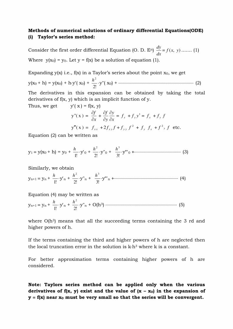
(i) Taylor’s series method:
Consider the first order differential Equation (O. D. En) ),(= yxfdx
dy....... (1)
Where y(x0) = y0. Let y = f(x) be a solution of equation (1).
Expanding y(x) i.e., f(x) in a Taylor’s series about the point x0, we get
y(x0 + h) = y(x0) + hy( x0) + !2
2h
y"( x0) + (2)
The derivatives in this expansion can be obtained by taking the total
derivatives of f(x, y) which is an implicit function of y.
Thus, we get y( x ) = f(x, y)
fffyffx
y
y
f
x
fyxyx +=+=+ = ) x (y" 1
fffffffff yxyyyyxxx
22 +++2+ = ) x (y etc.
Equation (2) can be written as
y1 = y(x0 + h) = y0 + !1
hy0 +
!2
2h
y"0 + !3
3h
y0 + (3)
Similarly, we obtain
yn+1 = yn + !1
hyn +
!2
2h
y"n + !3
3h
yn + (4)
Equation (4) may be written as
yn+1 = yn + !1
hyn +
!2
2h
y"n + O(h3) (5)
where O(h3) means that all the succeeding terms containing the 3 rd and
higher powers of h.
If the terms containing the third and higher powers of h are neglected then
the local truncation error in the solution is kh3 where k is a constant.
For better approximation terms containing higher powers of h are
considered.
Note: Taylors series method can be applied only when the various
derivatives of f(x, y) exist and the value of (x – x0) in the expansion of
y = f(x) near x0 must be very small so that the series will be convergent.
LAKIREDDY BALI REDDY COLLEGE OF ENGINEERING (AUTONOMOUS)
L.B.Reddy Nagar, Mylavaram – 521 230. Andhra Pradesh, INDIA
Approved by AICTE New Delhi Accredited by NBA, New Delhi & Certified by ISO 9001:2008
B. Tech I Year (II-Semester) May/ June 2014 T 264- Numerical Methods
ECE - B Section
UNIT – V Numerical Solutions of Faculty Name: N V Nagendram
Ordinary Differential Equations Tutorial-01
Problems on Taylor’s series
Problem #01 Form the Taylor’s series for y(x) , find y(0.1) correct to 4
decimal places if y(x) satisfies 1=)0(,1+= yxydx
dy. [Ans. 1.1053
Problem #02 Solve 0=)1(,+= yyxdx
dy and find y(1.1), y(1.2) by Taylor’s
series method. Compare the solution with exact solution.
[Ans.0.11033847; 0.2461077
Problem #03 Using Taylor’s series, find y at x = 0.1, 0.2 correct to 3
decimals given 0=)0(,3=2 yeydx
dy x . [Ans. y(0.1)= 0.349; y(0.2)= 0.811
Problem #04 Applying the Taylor’s series method, find the value of y(1.1)
and y(1.2) correct to three decimal places given that 1=)1(,= 3
1
yyxdx
dy
correct to 4 decimal places. [Ans. y(1.1)= 1.10681; y(1.2)= 1.22772
Problem #05 Find by Taylor’s series method, the value of y at x = 0.1,x = 0.2
to five decimal places given that 1=)0(,1= 2yyx
dx
dy .
[Ans. y(0.1)= 0.90033; y(0.2)= 0.80256
LAKIREDDY BALI REDDY COLLEGE OF ENGINEERING (AUTONOMOUS)
L.B.Reddy Nagar, Mylavaram – 521 230. Andhra Pradesh, INDIA
Approved by AICTE New Delhi Accredited by NBA, New Delhi & Certified by ISO 9001:2008
B. Tech I Year (II-Semester) May/ June 2014 T 264- Numerical Methods
ECE - B Section
UNIT – V Numerical Solutions of Faculty Name: N V Nagendram
Ordinary Differential Equations Tutorial-01 Problems on Taylor’s series
Problem #06 Find y(0.2), y(0.4) correct to 4 decimals 0=)0(,21= yxydx
dy .
[Ans. y(0.2)= 0.19475; y(0.4)= 0.35989
Problem #07 Solve 0=)0(,2+3= yyedx
dy xand find y at x = 0.1, 0.2 correct
to 3 decimal places. [Ans. y(0.1)= 0.3486955; y(0.2)= 0.8112658
Problem #08 Solve 1=)0(,+
=23
ye
yxx
dx
dyx
and find y(0.1),y(0.2),y(0.3)?
[Ans. y(0.1)= 1.0047;y(0.2)= 1.081812; y(0.3)= 1.03995
Problem #09 Solve 1=)1(,+= 3yxy
dx
dy find y(1.1), y(1.2), y(1.3) ?
[Ans. y(1.1)= 1.225;y(1.2)= 1.512; y(1.3)= 1.874
Problem #10 Solve 0=)8.1(,10
1+= =y 2
yyxdx
dy find y(2).[Ans.y(2)= 0.3809
Problem #11 Solve 4=)4(,+
1=
2y
yxdx
dyto obtain y(4.1), y(4.2)?
[Ans. y(4.1)= 4.005;y(4.2)= 4.0098
Problem #12 Solve 1=)0(,+= =y 2yyx
dx
dy and compute y(0.1) , y(0.2) ?
[Ans. y(0.1)= 1.1164;y(0.2)= 1.2725
Problem #13 Solve y(0.2) given 0=)0(,3+2= yeydx
dy xcompare the
numerical solution obtained with exact solution?
[Ans.y(0.2)=numerical 0.811;y(0.2)=exact 0.8112 Problem #14 Find y to 5 decimal places when x = 1.02 given that
2=)1(,1= yxydx
dy ? [Ans. y(1.02) = 2.02061
Problem #15 Find y(0.2), y(0.4) given 1=)0(,= 2yyx
dx
dy
[Ans. y(0.2) = 0.8511043;y(0.4)= 0.7750643
LAKIREDDY BALI REDDY COLLEGE OF ENGINEERING (AUTONOMOUS)
L.B.Reddy Nagar, Mylavaram – 521 230. Andhra Pradesh, INDIA
Approved by AICTE New Delhi Accredited by NBA, New Delhi & Certified by ISO 9001:2008
B. Tech I Year (II-Semester) May/ June 2014 T 264- Numerical Methods
ECE - B Section
UNIT – V Numerical Solutions of Faculty Name: N V Nagendram
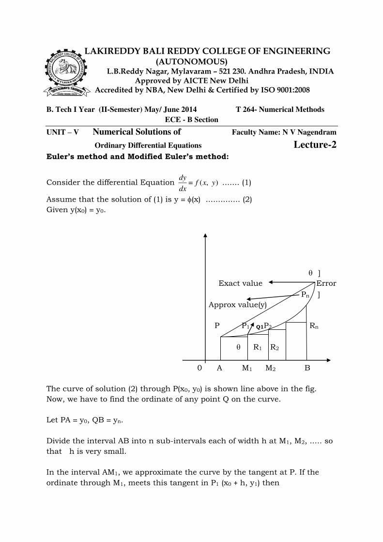
Ordinary Differential Equations Lecture-2 Euler’s method and Modified Euler’s method:
Consider the differential Equation ),(= yxfdx
dy ....... (1)
Assume that the solution of (1) is y = (x) .............. (2)
Given y(x0) = y0.
Exact value Error
Pn Approx value(y)
P P1 Q1P2 Rn
R1 R2
0 A M1 M2 B
The curve of solution (2) through P(x0, y0) is shown line above in the fig.
Now, we have to find the ordinate of any point Q on the curve.
Let PA = y0, QB = yn.
Divide the interval AB into n sub-intervals each of width h at M1, M2, ..... so
that h is very small.
In the interval AM1, we approximate the curve by the tangent at P. If the
ordinate through M1, meets this tangent in P1 (x0 + h, y1) then
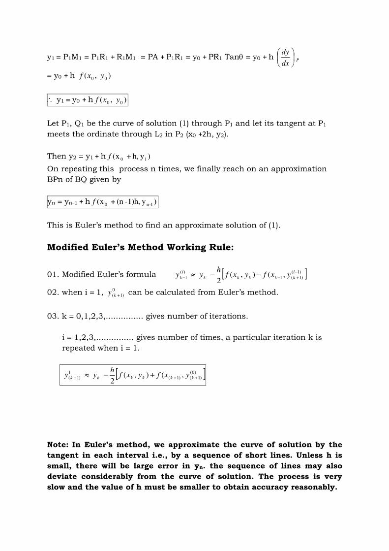
y1 = P1M1 = P1R1 + R1M1 = PA + P1R1 = y0 + PR1 Tan = y0 + h P
dx
dy
= y0 + h ),( 00 yxf
y1 = y0 + h ),( 00 yxf
Let P1, Q1 be the curve of solution (1) through P1 and let its tangent at P1
meets the ordinate through L2 in P2 (x0 +2h, y2).
Then y2 = y1 + h )y h, +x( 1 0f
On repeating this process n times, we finally reach on an approximation
BPn of BQ given by
yn = yn-1 + h )y 1)h,-(n +x( 1-n 0f
This is Euler’s method to find an approximate solution of (1).
Modified Euler’s Method Working Rule:
01. Modified Euler’s formula )1(
)1+(1
)(
1 ,(),(2
i
kkkkk
i
k yxfyxfh
yy
02. when i = 1, 0
)1+(ky can be calculated from Euler’s method.
03. k = 0,1,2,3,............... gives number of iterations.
i = 1,2,3,............... gives number of times, a particular iteration k is
repeated when i = 1.
)0(
)1+()1+(
1
)1+( ,(+),(2
kkkkkk yxfyxfh
yy
Note: In Euler’s method, we approximate the curve of solution by the
tangent in each interval i.e., by a sequence of short lines. Unless h is
small, there will be large error in yn. the sequence of lines may also
deviate considerably from the curve of solution. The process is very
slow and the value of h must be smaller to obtain accuracy reasonably.
LAKIREDDY BALI REDDY COLLEGE OF ENGINEERING (AUTONOMOUS)
L.B.Reddy Nagar, Mylavaram – 521 230. Andhra Pradesh, INDIA
Approved by AICTE New Delhi Accredited by NBA, New Delhi & Certified by ISO 9001:2008
B. Tech I Year (II-Semester) May/ June 2014 T 264- Numerical Methods
ECE - B Section
UNIT – V Numerical Solutions of Faculty Name: N V Nagendram
Ordinary Differential Equations Tutorial-02
Problems on EULER’S METHOD
Problem #01 Using Euler’s method, find an appropriate value of y
corresponding to x = 1 given that )+(= yxdx
dy and y(0) = 1?
Problem #02 Using Euler’s method, find an appropriate value of y
corresponding to x =0.3 given that )+(= yxdx
dy and y(0) = 1?
Problem #03 Using Euler’s method, find an appropriate value of y(0.02) = 1
given that )+(= 2yx
dx
dy and y(0) = 1?
Problem #04 Solve by Euler’s method, the differential equation )+(
)(=
xy
xy
dx
dy
with the initial condition y(0) = 1 and find an appropriate value of y
corresponding to x = 0.1 correct to four decimal places?
Problem #05 Given ydx
dy= and y(0) = 1 determine the values of y at x =
(0.01) (0.01) (0.04) by Euler’s method. Compare the values with exact values?
Problem #06 Solve )1(= ydx
dy given y(0) = 0 using modified Euler’s method
and tabulate the solutions at x = 0.1, 0.2 and 0.3 Compare your results with exact solutions?
LAKIREDDY BALI REDDY COLLEGE OF ENGINEERING (AUTONOMOUS)
L.B.Reddy Nagar, Mylavaram – 521 230. Andhra Pradesh, INDIA
Approved by AICTE New Delhi Accredited by NBA, New Delhi & Certified by ISO 9001:2008
B. Tech I Year (II-Semester) May/ June 2014 T 264- Numerical Methods
ECE - B Section
UNIT – V Numerical Solutions of Faculty Name: N V Nagendram
Ordinary Differential Equations Lecture-3 Picard’s method of successive approximation:
Consider the differential Equation ),(= yxfdx
dy, y(x0) = y0.
Integrating the differential Equation between x0 and x, x
x
x
x
dxyxfdy
00
),(=
y(x) – y(x0) x
x
dxyxf
0
),(= .................................................................... (1)
Equation (1) is known as an integral equation since the dependent variable y occurs in the function f(x, y) on the right hand side under the sign of integration. The first approximation y1 is obtained by replacing y by y0 in f(x, y) in equation (1)
x
x
dxyxfyy
0
),(+= 001 .................................................................... (2)
The second approximation y2 is obtained by replacing y by y1 in f(x, y) in equation (1)
x
x
dxyxfyy
0
),(+= 102 .................................................................... (3)
The successive approximations of y are given by
x
x
dxyxfyy
0
),(+= 203
-------------------------------------------------------------------------------------- --------------------------------------------------------------------------------------
x
x
nn dxyxfyy
0
),(+= 10 The process of iteration is stopped when any two
values of iteration are approximately the same. If x is large the convergence
is slow.
LAKIREDDY BALI REDDY COLLEGE OF ENGINEERING (AUTONOMOUS)
L.B.Reddy Nagar, Mylavaram – 521 230. Andhra Pradesh, INDIA
Approved by AICTE New Delhi Accredited by NBA, New Delhi & Certified by ISO 9001:2008
B. Tech I Year (II-Semester) May/ June 2014 T 264- Numerical Methods
ECE - B Section
UNIT – V Numerical Solutions of Faculty Name: N V Nagendram
Ordinary Differential Equations Tutorial-03
Problems on PICARD’S METHOD
Problem #01 Solve the equation )1+(= xydx
dy, y(0) = 1 by Picard’s method of
successive approximation and hence find y when x = 0.1?
Problem #02 Use Picard’s method to obtain y when x = 0.2 correct to five
decimal places given )(= yxdx
dy , y(0) = 1. Check your answer by finding the
exact particular solution?
Problem #03 Use Picard’s method of approximation to find y when x = 0.1, x
= 0.2 given )+(= 2yx
dx
dy, y(0) = 0?
Problem #04 Use Picard’s process of successive approximations obtain a
solution of the equation )x+(= 22y
dx
dy, y(0) = 1?
Problem #04 Solve ydx
dy= , y(0) = 1 by Picard’s method and compare the
solution with exact solution?
LAKIREDDY BALI REDDY COLLEGE OF ENGINEERING (AUTONOMOUS)
L.B.Reddy Nagar, Mylavaram – 521 230. Andhra Pradesh, INDIA
Approved by AICTE New Delhi Accredited by NBA, New Delhi & Certified by ISO 9001:2008
B. Tech I Year (II-Semester) May/ June 2014 T 264- Numerical Methods
ECE - B Section
UNIT – V Numerical Solutions of Faculty Name: N V Nagendram
Ordinary Differential Equations Lecture-4
Runge – Kutta Method
The basic disadvantage of Taylor’s series method lies in the calculation of higher order total derivatives of Y. Euler’s method requires the smallness of
h for attaining reasonable accuracy. In order to overcomes these
disadvantages, the Runge – Kutta methods are designed to obtain greater
accuracy and at the same time to avoid the need for calculating higher order
derivatives. The advantage of these methods is that the functional values
only required at some selected points on the sub-interval.
I st order Runge – Kutta Method:
Consider the differential equation ),(= yxfdx
dy, y(x0) = y0
y1 = y(x0 + h)
Expanding by Taylor’s series
y1 = y(x0 + h) = y0 + !1
hy0 +
!2
2h
y"0 + !3
3h
y0 +
Also by Euler’s method
y1 = y0 + h f(x0 , y0) = y0 + hy0
It follows that the Euler’s method agrees with the Taylor’s series solution up
to the term in h.
Hence, Euler’s method is the Runge – Kutta method of the Ist order.
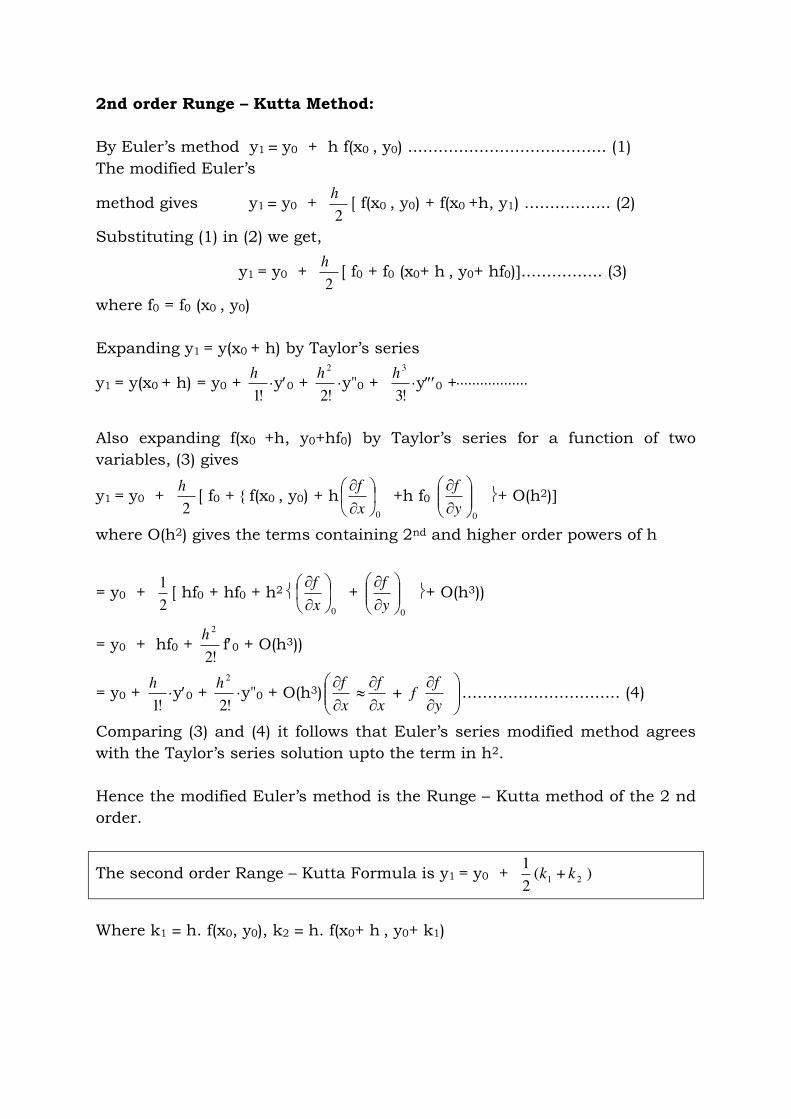
2nd order Runge – Kutta Method:
By Euler’s method y1 = y0 + h f(x0 , y0) ....................................... (1)
The modified Euler’s
method gives y1 = y0 + 2
h[ f(x0 , y0) + f(x0 +h, y1) ................. (2)
Substituting (1) in (2) we get,
y1 = y0 + 2
h[ f0 + f0 (x0+ h , y0+ hf0)................ (3)
where f0 = f0 (x0 , y0)
Expanding y1 = y(x0 + h) by Taylor’s series
y1 = y(x0 + h) = y0 + !1
hy0 +
!2
2h
y"0 + !3
3h
y0 +
Also expanding f(x0 +h, y0+hf0) by Taylor’s series for a function of two
variables, (3) gives
y1 = y0 + 2
h[ f0 + { f(x0 , y0) + h
0
x
f+h f0
0
y
f+ O(h2)
where O(h2) gives the terms containing 2nd and higher order powers of h
= y0 + 2
1[ hf0 + hf0 + h2
0
x
f+
0
y
f+ O(h3))
= y0 + hf0 + !2
2h
f0 + O(h3))
= y0 + !1
hy0 +
!2
2h
y"0 + O(h3)
y
ff
x
f
x
f+ ............................... (4)
Comparing (3) and (4) it follows that Euler’s series modified method agrees with the Taylor’s series solution upto the term in h2.
Hence the modified Euler’s method is the Runge – Kutta method of the 2 nd
order.
The second order Range – Kutta Formula is y1 = y0 + )+(2
121 kk
Where k1 = h. f(x0, y0), k2 = h. f(x0+ h , y0+ k1)
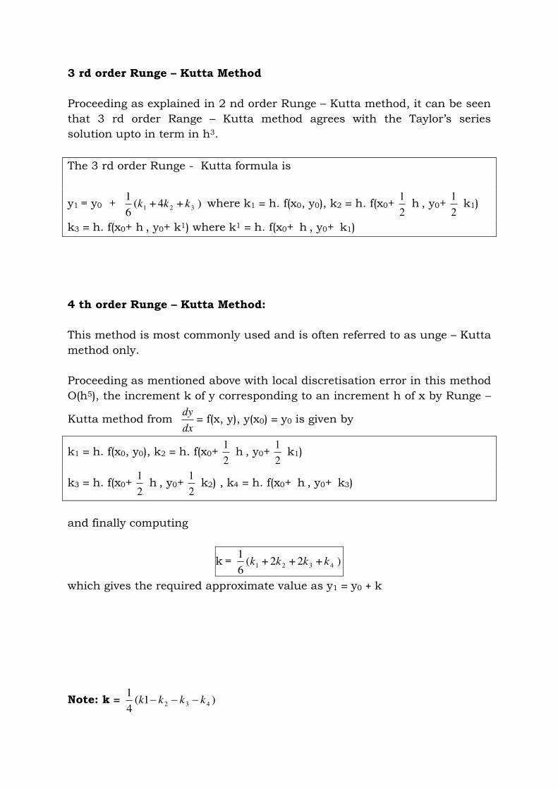
3 rd order Runge – Kutta Method
Proceeding as explained in 2 nd order Runge – Kutta method, it can be seen
that 3 rd order Range – Kutta method agrees with the Taylor’s series solution upto in term in h3.
The 3 rd order Runge - Kutta formula is
y1 = y0 + )+4+(6
1321 kkk where k1 = h. f(x0, y0), k2 = h. f(x0+
2
1 h , y0+
2
1 k1)
k3 = h. f(x0+ h , y0+ k1) where k1 = h. f(x0+ h , y0+ k1)
4 th order Runge – Kutta Method:
This method is most commonly used and is often referred to as unge – Kutta
method only.
Proceeding as mentioned above with local discretisation error in this method
O(h5), the increment k of y corresponding to an increment h of x by Runge –
Kutta method from dx
dy= f(x, y), y(x0) = y0 is given by
k1 = h. f(x0, y0), k2 = h. f(x0+
2
1 h , y0+
2
1 k1)
k3 = h. f(x0+
2
1 h , y0+
2
1 k2) , k4 = h. f(x0+ h , y0+ k3)
and finally computing
k = )+2+2+(6
14321 kkkk
which gives the required approximate value as y1 = y0 + k
Note: k = )1(4
1432 kkkk
LAKIREDDY BALI REDDY COLLEGE OF ENGINEERING (AUTONOMOUS)
L.B.Reddy Nagar, Mylavaram – 521 230. Andhra Pradesh, INDIA
Approved by AICTE New Delhi Accredited by NBA, New Delhi & Certified by ISO 9001:2008
B. Tech I Year (II-Semester) May/ June 2014 T 264- Numerical Methods
ECE - B Section
UNIT – V Numerical Solutions of Faculty Name: N V Nagendram
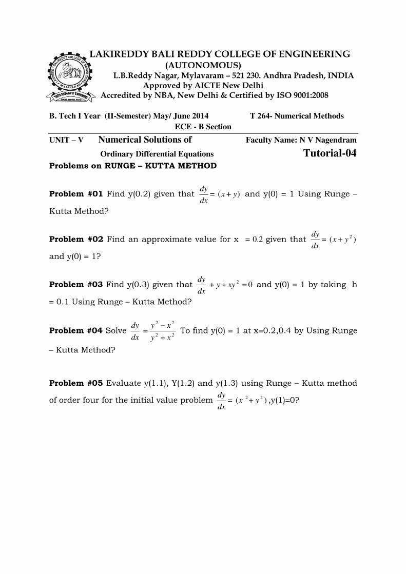
Ordinary Differential Equations Tutorial-04 Problems on RUNGE – KUTTA METHOD
Problem #01 Find y(0.2) given that )+(= yxdx
dy and y(0) = 1 Using Runge –
Kutta Method?
Problem #02 Find an approximate value for x = 0.2 given that )+(= 2yx
dx
dy
and y(0) = 1?
Problem #03 Find y(0.3) given that 0=++ 2xyy
dx
dy and y(0) = 1 by taking h
= 0.1 Using Runge – Kutta Method?
Problem #04 Solve 22
22
+=
xy
xy
dx
dy To find y(0) = 1 at x=0.2,0.4 by Using Runge
– Kutta Method?
Problem #05 Evaluate y(1.1), Y(1.2) and y(1.3) using Runge – Kutta method
of order four for the initial value problem )+(= 22yx
dx
dy,y(1)=0?
LAKIREDDY BALI REDDY COLLEGE OF ENGINEERING (AUTONOMOUS)
L.B.Reddy Nagar, Mylavaram – 521 230. Andhra Pradesh, INDIA
Approved by AICTE New Delhi Accredited by NBA, New Delhi & Certified by ISO 9001:2008
B. Tech I Year (II-Semester) May/ June 2014 T 264- Numerical Methods
ECE - B Section
UNIT – V Numerical Solutions of Faculty Name: N V Nagendram
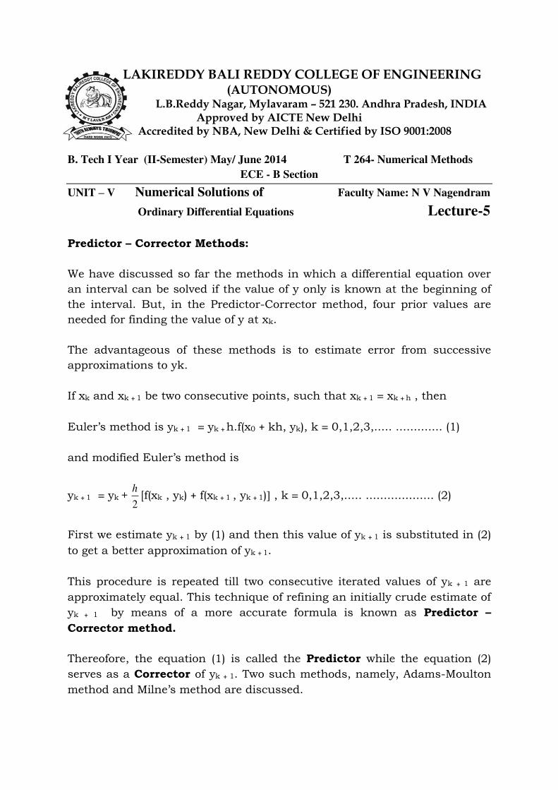
Ordinary Differential Equations Lecture-5
Predictor – Corrector Methods:
We have discussed so far the methods in which a differential equation over
an interval can be solved if the value of y only is known at the beginning of
the interval. But, in the Predictor-Corrector method, four prior values are
needed for finding the value of y at xk.
The advantageous of these methods is to estimate error from successive
approximations to yk.
If xk and xk + 1 be two consecutive points, such that xk + 1 = xk + h , then
Euler’s method is yk + 1 = yk + h.f(x0 + kh, yk), k = 0,1,2,3,..... ............. (1)
and modified Euler’s method is
yk + 1 = yk +
2
h[f(xk , yk) + f(xk + 1 , yk + 1) , k = 0,1,2,3,..... ................... (2)
First we estimate yk + 1 by (1) and then this value of yk + 1 is substituted in (2)
to get a better approximation of yk + 1.
This procedure is repeated till two consecutive iterated values of yk + 1 are
approximately equal. This technique of refining an initially crude estimate of
yk + 1 by means of a more accurate formula is known as Predictor – Corrector method.
Thereofore, the equation (1) is called the Predictor while the equation (2)
serves as a Corrector of yk + 1. Two such methods, namely, Adams-Moulton
method and Milne’s method are discussed.
LAKIREDDY BALI REDDY COLLEGE OF ENGINEERING (AUTONOMOUS)
L.B.Reddy Nagar, Mylavaram – 521 230. Andhra Pradesh, INDIA
Approved by AICTE New Delhi Accredited by NBA, New Delhi & Certified by ISO 9001:2008
B. Tech I Year (II-Semester) May/ June 2014 T 264- Numerical Methods
ECE - B Section
UNIT – V Numerical Solutions of Faculty Name: N V Nagendram
Ordinary Differential Equations Lecture-6
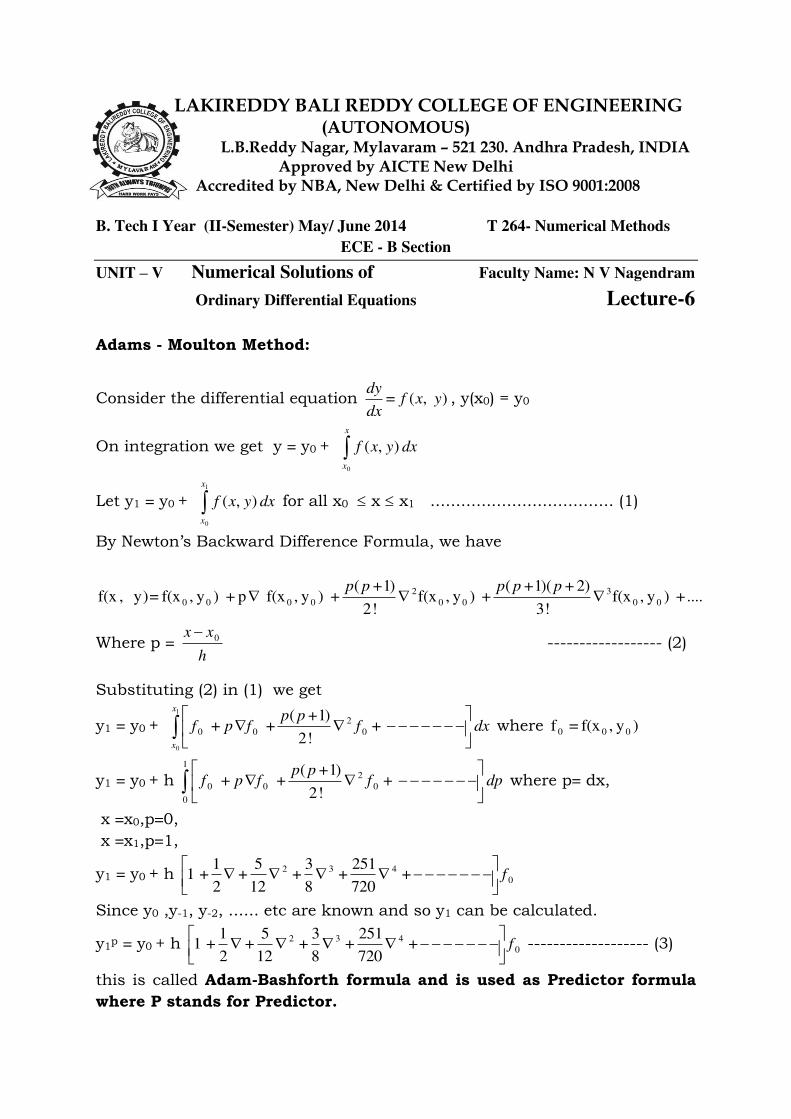
Adams - Moulton Method:
Consider the differential equation ),(= yxfdx
dy, y(x0) = y0
On integration we get y = y0 + x
x
dxyxf
0
),(
Let y1 = y0 + 1
0
),(
x
x
dxyxf for all x0 x x1 .................................... (1)
By Newton’s Backward Difference Formula, we have
....+ )y,f(x!3
)2+)(1+(+ )y,f(x
!2
)1+(+ )y,f(x p + )y,f(x = y),f(x 00
3
00
2
0000 ppppp
Where p = h
xx 0 ------------------ (2)
Substituting (2) in (1) we get
y1 = y0 + dxfpp
fpf
x
x
1
0
+!2
)1+(++ 0
2
00 where )y,f(x =f 000
y1 = y0 + h dpfpp
fpf
1
0
0
2
00 +!2
)1+(++ where p= dx,
x =x0,p=0,
x =x1,p=1,
y1 = y0 + h 0
432 +720
251+
8
3+
12
5+
2
1+1 f
Since y0 ,y-1, y-2, ...... etc are known and so y1 can be calculated.
y1p = y0 + h 0
432 +720
251+
8
3+
12
5+
2
1+1 f
------------------- (3)
this is called Adam-Bashforth formula and is used as Predictor formula
where P stands for Predictor.
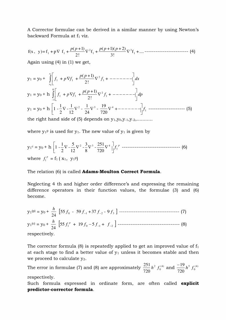
A Corrector formulae can be derived in a similar manner by using Newton’s backward Formula at f1 viz.
....+f!3
)2+)(1+(+f
!2
)1+(+ f p + f = y),f(x 1
3
1
2
11 ppppp
------------------------ (4)
Again using (4) in (1) we get,
y1 = y0 + dxfpp
fpf
x
x
1
0
+!2
)1+(++ 1
2
11
y1 = y0 + h dpfpp
fpf
0
1
1
2
11 +!2
)1+(++
y1 = y0 + h 1
432 +720
19 -
24
1 -
12
1-
2
1-1 f
-------------------- (5)
the right hand side of (5) depends on y1,y0,y-1,y-2,...........
where y1p is used for y1. The new value of y1 is given by
y1c = y0 + h
pf1
432
720
251-
8
3-
12
5-
2
1-1
-------------------------------- (6)
where p
f1 = f1 ( x1, y1p)
The relation (6) is called Adams-Moulton Correct Formula.
Neglecting 4 th and higher order difference’s and expressing the remaining difference operators in their function values, the formulae (3) and (6)
become.
y1(p) = y0 +
24
h 3210 9-37+59 -55 ffff --------------------------------- (7)
y1(c) = y0 +
24
h 2101 +519 +55 ffff
p ---------------------------------- (8)
respectively.
The corrector formula (8) is repeatedly applied to get an improved value of f1
at each stage to find a better value of y1 unless it becomes stable and then
we proceed to calculate y2.
The error in formulae (7) and (8) are approximately )4(
0
2
720
251fh and )4(
0
5
720
19fh
respectively.
Such formula expressed in ordinate form, are often called explicit
predictor-corrector formula.
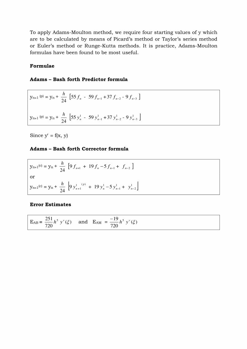
To apply Adams-Moulton method, we require four starting values of y which
are to be calculated by means of Picard’s method or Taylor’s series method or Euler’s method or Runge-Kutta methods. It is practice, Adams-Moulton
formulas have been found to be most useful.
Formulae
Adams – Bash forth Predictor formula
yn+1 (p) = yn +
24
h 321 9-37+59 -55 nnnn ffff
yn+1 (p) = yn +
24
h 1
3
1
2
1
1
1 9-37+59 -55 nnnn yyyy
Since y = f(x, y)
Adams – Bash forth Corrector formula
yn+1(c) = yn +
24
h 211+ +519 +9 nnnn ffff
or
yn+1(c) = yn +
24
h 1
2
1
1
1)(1
1+ +519 +9 nnn
p
n yyyy
Error Estimates
EAB = )(720
251 5 vyh and EAM = )(
720
19 5 vyh
LAKIREDDY BALI REDDY COLLEGE OF ENGINEERING (AUTONOMOUS)
L.B.Reddy Nagar, Mylavaram – 521 230. Andhra Pradesh, INDIA
Approved by AICTE New Delhi Accredited by NBA, New Delhi & Certified by ISO 9001:2008
B. Tech I Year (II-Semester) May/ June 2014 T 264- Numerical Methods
ECE - B Section
UNIT – V Numerical Solutions of Faculty Name: N V Nagendram
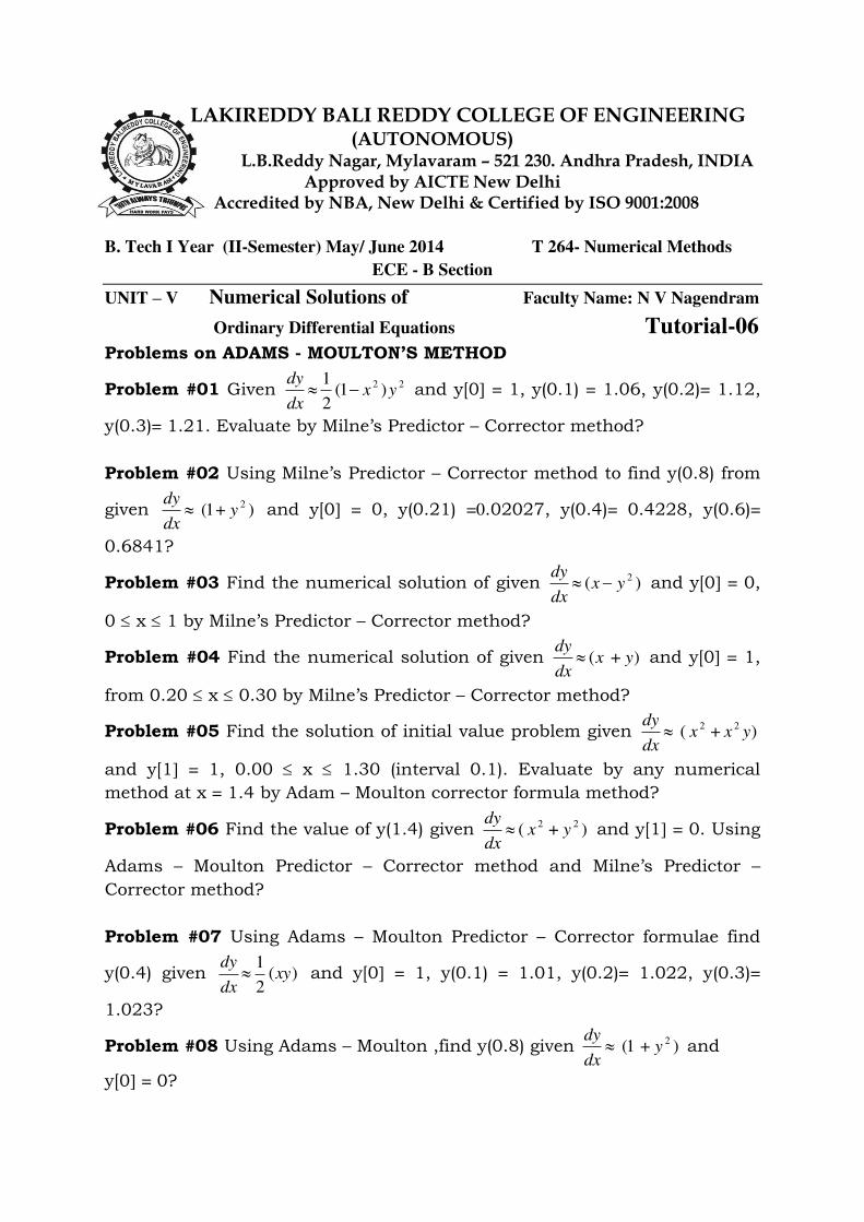
Ordinary Differential Equations Tutorial-06 Problems on ADAMS - MOULTON’S METHOD
Problem #01 Given 22 )1(2
1yx
dx
dy and y[0 = 1, y(0.1) = 1.06, y(0.2)= 1.12,
y(0.3)= 1.21. Evaluate by Milne’s Predictor – Corrector method?
Problem #02 Using Milne’s Predictor – Corrector method to find y(0.8) from
given )+1( 2y
dx
dy and y[0 = 0, y(0.21) =0.02027, y(0.4)= 0.4228, y(0.6)=
0.6841?
Problem #03 Find the numerical solution of given )( 2yx
dx
dy and y[0 = 0,
0 x 1 by Milne’s Predictor – Corrector method?
Problem #04 Find the numerical solution of given )+( yxdx
dy and y[0 = 1,
from 0.20 x 0.30 by Milne’s Predictor – Corrector method?
Problem #05 Find the solution of initial value problem given )+( 22yxx
dx
dy
and y[1 = 1, 0.00 x 1.30 (interval 0.1). Evaluate by any numerical
method at x = 1.4 by Adam – Moulton corrector formula method?
Problem #06 Find the value of y(1.4) given )+( 22yx
dx
dy and y[1 = 0. Using
Adams – Moulton Predictor – Corrector method and Milne’s Predictor –
Corrector method?
Problem #07 Using Adams – Moulton Predictor – Corrector formulae find
y(0.4) given )(2
1xy
dx
dy and y[0 = 1, y(0.1) = 1.01, y(0.2)= 1.022, y(0.3)=
1.023?
Problem #08 Using Adams – Moulton ,find y(0.8) given )+1( 2y
dx
dy and
y[0 = 0?
LAKIREDDY BALI REDDY COLLEGE OF ENGINEERING (AUTONOMOUS)
L.B.Reddy Nagar, Mylavaram – 521 230. Andhra Pradesh, INDIA
Approved by AICTE New Delhi Accredited by NBA, New Delhi & Certified by ISO 9001:2008
B. Tech I Year (II-Semester) May/ June 2014 T 264- Numerical Methods
ECE - B Section
UNIT – V Numerical Solutions of Faculty Name: N V Nagendram
Ordinary Differential Equations Lecture-7
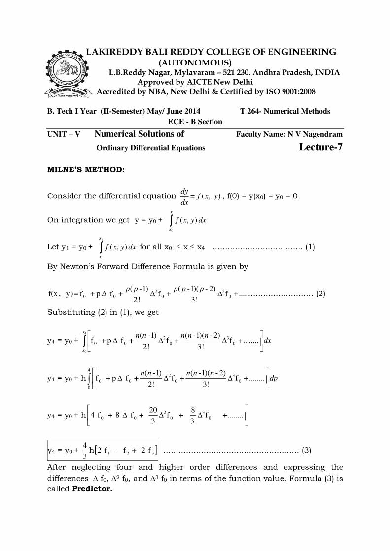
MILNE’S METHOD:
Consider the differential equation ),(= yxfdx
dy, f(0) = y(x0) = y0 = 0
On integration we get y = y0 + x
x
dxyxf
0
),(
Let y1 = y0 + 4
0
),(
x
x
dxyxf for all x0 x x4 .................................... (1)
By Newton’s Forward Difference Formula is given by
....+f!3
)2-)(1-(+f
!2
)1-(+ f p + f = y),f(x 0
3
0
2
00 ppppp
.......................... (2)
Substituting (2) in (1), we get
y4 = y0 +
4
0
........+f!3
)2-)(1-(+f
!2
)1-(+ f p + f 0
3
0
2
00
x
x
dxnnnnn
y4 = y0 + h
4
0
0
3
0
2
00 ........+f!3
)2-)(1-(+f
!2
)1-(+ f p + f dp
nnnnn
y4 = y0 + h
........+f
3
8+f
3
20+ f 8 + f4 0
3
0
2
00
y4 = y0 + 3
4h 321 f2+ f - f2 ...................................................... (3)
After neglecting four and higher order differences and expressing the
differences f0, 2 f0, and 3 f0 in terms of the function value. Formula (3) is
called Predictor.
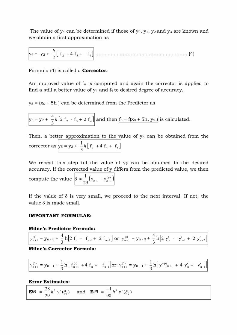
The value of y4 can be determined if those of y0, y1, y2 and y3 are known and
we obtain a first approximation as
y4 = y2 + 2
h 432 f+ f 4+ f ............................................................ (4)
Formula (4) is called a Corrector.
An improved value of f4 is computed and again the corrector is applied to
find a still a better value of y4 and f4 to desired degree of accuracy,
y5 = (x0 + 5h ) can be determined from the Predictor as
y5 = y2 + h3
4 432 f2+ f - f2 and then f5 = f(x0 + 5h, y5 ) is calculated.
Then, a better approximation to the value of y5 can be obtained from the
corrector as y5 = y3 + h3
1 543 f+ f4 + f
We repeat this step till the value of y5 can be obtained to the desired
accuracy. If the corrected value of y differs from the predicted value, we then
compute the value )(
1+1+29
1 p
nn yy
If the value of is very small, we proceed to the next interval. If not, the
value is made small.
IMPORTANT FORMULAE:
Milne’s Predictor Formula: (p)
1+ny = yn - 3 + 3
4h 2-n1-nn f2+ f - f2 or (p)
1+ny = yn - 3 + 3
4h 2-n1-nn y2+ y - y2
Milne’s Corrector Formula:
(C)
1+ny = yn - 1 + 3
1h 1-nn
(p)
1+n f+ f 4+ f or (C)
1+ny = yn - 1 + 3
1h 1-nn1+n
(p) y+ y 4+ y
Error Estimates:
E(p) = )(29
281
5 vyh and E(C) = )(
90
12
5 vyh
LAKIREDDY BALI REDDY COLLEGE OF ENGINEERING (AUTONOMOUS)
L.B.Reddy Nagar, Mylavaram – 521 230. Andhra Pradesh, INDIA
Approved by AICTE New Delhi Accredited by NBA, New Delhi & Certified by ISO 9001:2008
B. Tech I Year (II-Semester) May/ June 2014 Subject: T 264- Numerical Methods
ECE – B Section
UNIT – I Important Questions Faculty Name: N V Nagendram
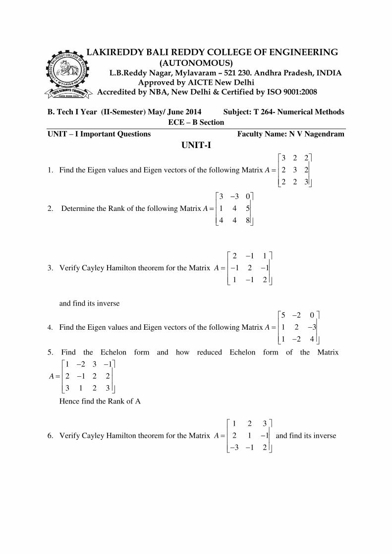
UNIT-I
1. Find the Eigen values and Eigen vectors of the following Matrix
3 2 2
2 3 2
2 2 3
A
2. Determine the Rank of the following Matrix
3 3 0
1 4 5
4 4 8
A
3. Verify Cayley Hamilton theorem for the Matrix
2 1 1
1 2 1
1 1 2
A
and find its inverse
4. Find the Eigen values and Eigen vectors of the following Matrix
5 2 0
1 2 3
1 2 4
A
5. Find the Echelon form and how reduced Echelon form of the Matrix
1 2 3 1
2 1 2 2
3 1 2 3
A
Hence find the Rank of A
6. Verify Cayley Hamilton theorem for the Matrix
1 2 3
2 1 1
3 1 2
A
and find its inverse
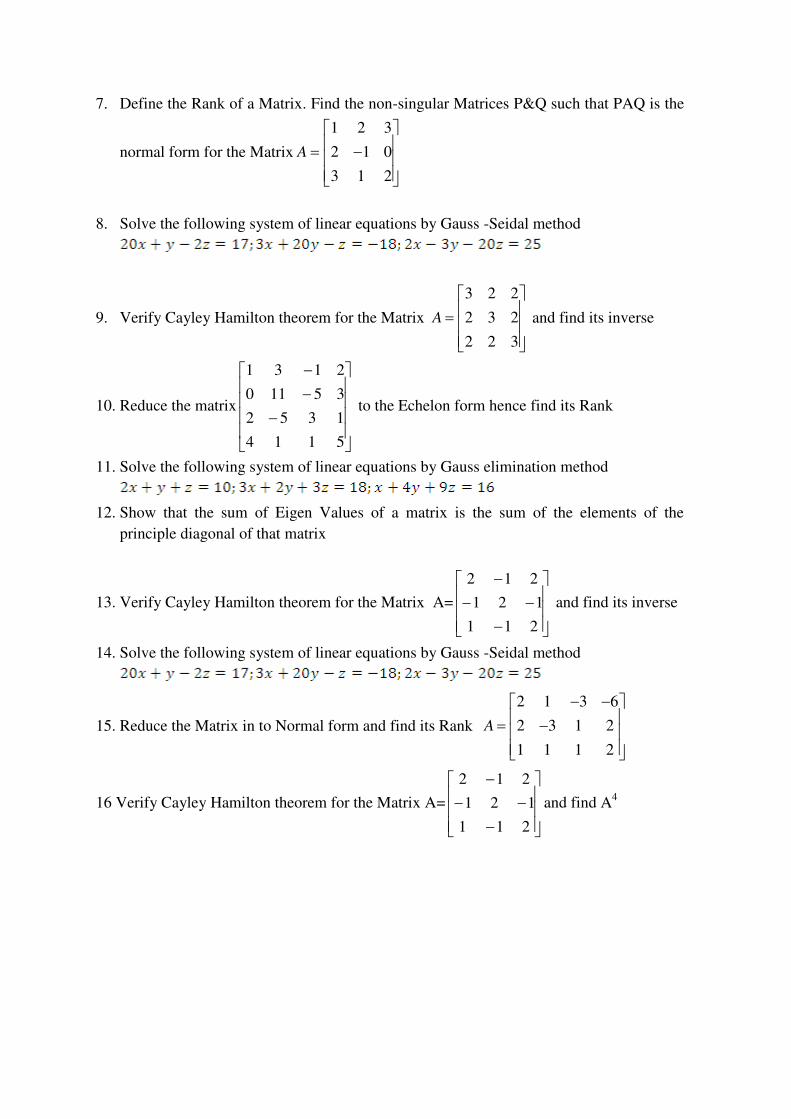
7. Define the Rank of a Matrix. Find the non-singular Matrices P&Q such that PAQ is the
normal form for the Matrix
1 2 3
2 1 0
3 1 2
A
8. Solve the following system of linear equations by Gauss -Seidal method
9. Verify Cayley Hamilton theorem for the Matrix
3 2 2
2 3 2
2 2 3
A
and find its inverse
10. Reduce the matrix
5114
1352
35110
2131
to the Echelon form hence find its Rank
11. Solve the following system of linear equations by Gauss elimination method
12. Show that the sum of Eigen Values of a matrix is the sum of the elements of the
principle diagonal of that matrix
13. Verify Cayley Hamilton theorem for the Matrix A=
211
121
212
and find its inverse
14. Solve the following system of linear equations by Gauss -Seidal method
15. Reduce the Matrix in to Normal form and find its Rank
2 1 3 6
2 3 1 2
1 1 1 2
A
16 Verify Cayley Hamilton theorem for the Matrix A=
211
121
212
and find A4
LAKIREDDY BALI REDDY COLLEGE OF ENGINEERING (AUTONOMOUS)
L.B.Reddy Nagar, Mylavaram – 521 230. Andhra Pradesh, INDIA
Approved by AICTE New Delhi Accredited by NBA, New Delhi & Certified by ISO 9001:2008
B. Tech I Year (II-Semester) May/ June 2014 Subject: T 264- Numerical Methods
ECE – B Section
UNIT – II Important Questions Faculty Name: N V Nagendram
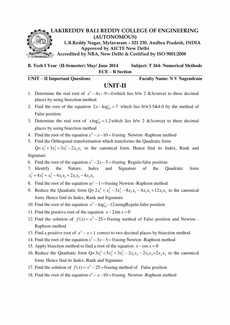
UNIT-II
1. Determine the real root of 3 4 9 0x x which lies b/w 2 &3corrcet to three decimal
places by using bisection method
2. Find the root of the equation 102 log 7xx which lies b/w3.5&4.0 by the method of
False position
3. Determine the real root of 10log 1.2xx which lies b/w 2 &3corrcet to three decimal
places by using bisection method
4. Find the root of the equation 4 10 0x x using Newton -Raphson method
5. Find the Orthogonal transformation which transforms the Quadratic form
Q= 2 2 2
1 2 3 2 33 3 2x x x x x to the canonical form. Hence find its Index, Rank and
Signature
6. Find the root of the equation 3 2 5 0x x using Regula-false position
7. Identify the Nature, Index and Signature of the Quadratic form 2 2 2
1 2 3 1 2 1 3 2 34 4 2 4x x x x x x x x x
8. Find the root of the equation 1 0xxe using Newton -Raphson method
9. Reduce the Quadratic form Q= 2 2 2
1 2 3 2 3 3 1 1 22 3 8 4 12x x x x x x x x x to the canonical
form. Hence find its Index, Rank and Signature
10. Find the root of the equation 2
10log 12xx usingRegula-false position
11. Find the positive root of the equation 2sin 0x x
12. Find the solution of 2( ) 25 0f x x using method of False position and Newton -
Raphson method
13. Find a positive root of 13 xx correct to two decimal places by bisection method
14. Find the root of the equation 2 3 5 0x x using Newton -Raphson method
15. Apply bisection method to find a root of the equation 0cos xx
16. Reduce the Quadratic form Q= 323121
2
3
2
2
2
1 222353 xxxxxxxxx to the canonical
form. Hence find its Index, Rank and Signature
17. Find the solution of 2( ) 25 0f x x using method of False position
18. Find the root of the equation 4 10 0x x using Newton -Raphson method
LAKIREDDY BALI REDDY COLLEGE OF ENGINEERING (AUTONOMOUS)
L.B.Reddy Nagar, Mylavaram – 521 230. Andhra Pradesh, INDIA
Approved by AICTE New Delhi Accredited by NBA, New Delhi & Certified by ISO 9001:2008
B. Tech I Year (II-Semester) May/ June 2014 Subject: T 264- Numerical Methods
ECE – B Section
UNIT – III Important Questions Faculty Name: N V Nagendram
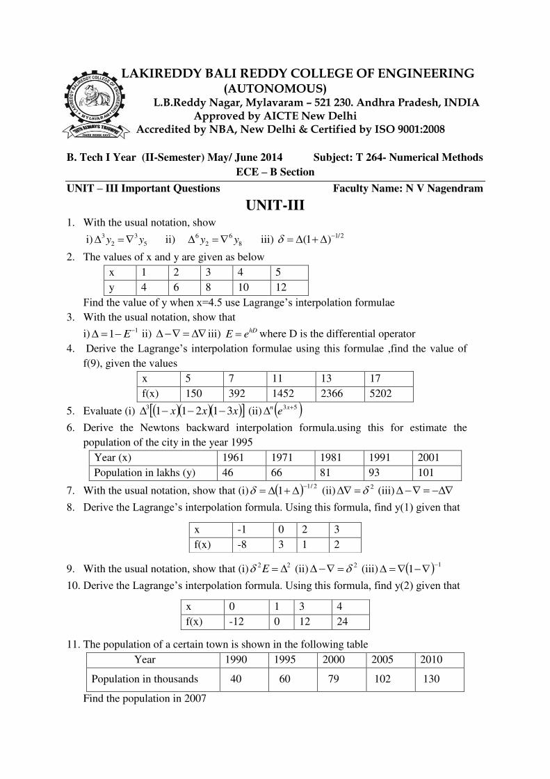
UNIT-III 1. With the usual notation, show
i) 3 3
2 5y y ii) 6 6
2 8y y iii) 1/2(1 )
2. The values of x and y are given as below
x 1 2 3 4 5
y 4 6 8 10 12
Find the value of y when x=4.5 use Lagrange’s interpolation formulae
3. With the usual notation, show that
i) 11 E ii) iii) hD
E e where D is the differential operator
4. Derive the Lagrange’s interpolation formulae using this formulae ,find the value of
f(9), given the values
x 5 7 11 13 17
f(x) 150 392 1452 2366 5202
5. Evaluate (i) xxx 312113 (ii) 53 xne
6. Derive the Newtons backward interpolation formula.using this for estimate the
population of the city in the year 1995
Year (x) 1961 1971 1981 1991 2001
Population in lakhs (y) 46 66 81 93 101
7. With the usual notation, show that (i) 2/11
(ii)2 (iii)
8. Derive the Lagrange’s interpolation formula. Using this formula, find y(1) given that
9. With the usual notation, show that (i)22 E (ii)
2 (iii) 11
10. Derive the Lagrange’s interpolation formula. Using this formula, find y(2) given that
11. The population of a certain town is shown in the following table
Year 1990 1995 2000 2005 2010
Population in thousands 40 60 79 102 130
Find the population in 2007
x -1 0 2 3
f(x) -8 3 1 2
x 0 1 3 4
f(x) -12 0 12 24
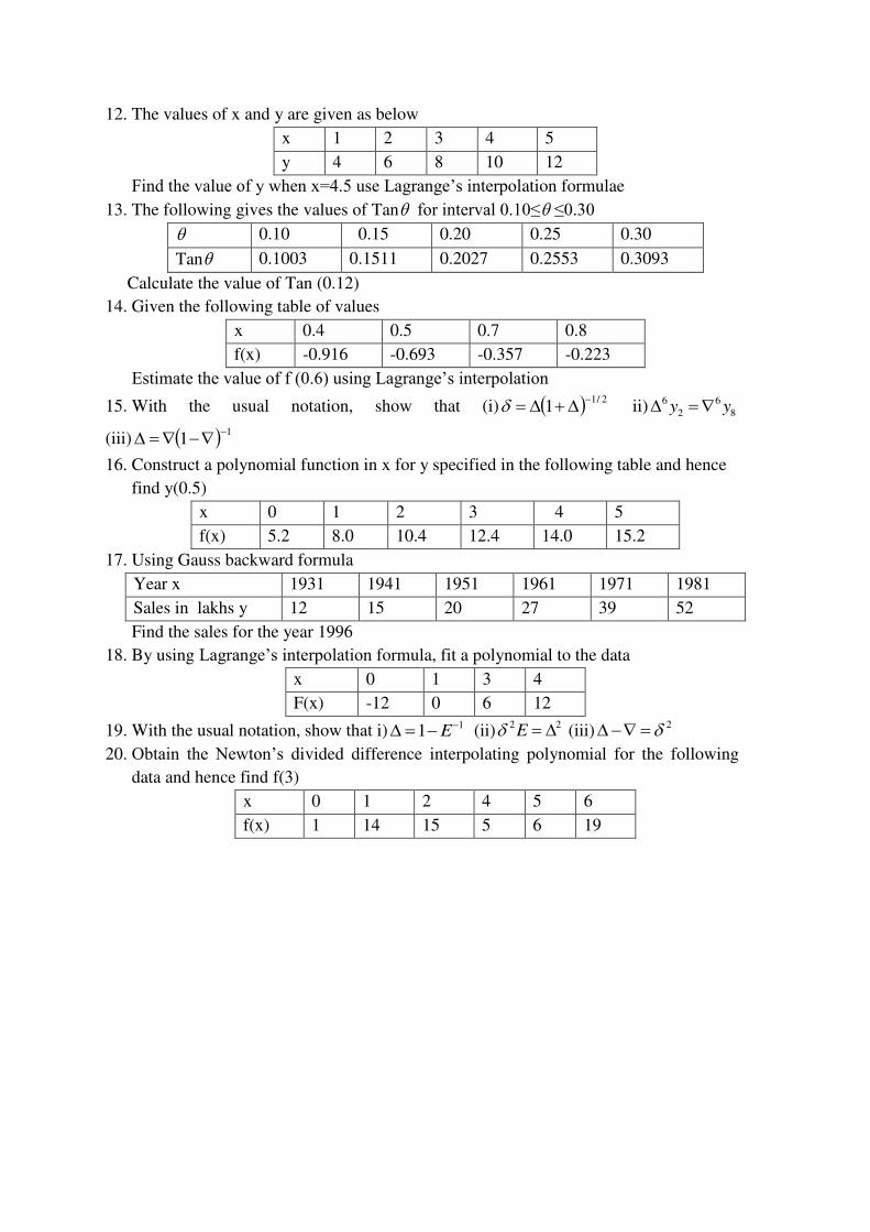
12. The values of x and y are given as below
x 1 2 3 4 5
y 4 6 8 10 12
Find the value of y when x=4.5 use Lagrange’s interpolation formulae
13. The following gives the values of Tan for interval 0.10≤ ≤0.30
0.10 0.15 0.20 0.25 0.30
Tan 0.1003 0.1511 0.2027 0.2553 0.3093
Calculate the value of Tan (0.12)
14. Given the following table of values
x 0.4 0.5 0.7 0.8
f(x) -0.916 -0.693 -0.357 -0.223
Estimate the value of f (0.6) using Lagrange’s interpolation
15. With the usual notation, show that (i) 2/11
ii) 6 6
2 8y y
(iii) 11
16. Construct a polynomial function in x for y specified in the following table and hence
find y(0.5)
x 0 1 2 3 4 5
f(x) 5.2 8.0 10.4 12.4 14.0 15.2
17. Using Gauss backward formula
Year x 1931 1941 1951 1961 1971 1981
Sales in lakhs y 12 15 20 27 39 52
Find the sales for the year 1996
18. By using Lagrange’s interpolation formula, fit a polynomial to the data
x 0 1 3 4
F(x) -12 0 6 12
19. With the usual notation, show that i) 11 E (ii)
22 E (iii)2
20. Obtain the Newton’s divided difference interpolating polynomial for the following
data and hence find f(3)
x 0 1 2 4 5 6
f(x) 1 14 15 5 6 19
LAKIREDDY BALI REDDY COLLEGE OF ENGINEERING (AUTONOMOUS)
L.B.Reddy Nagar, Mylavaram – 521 230. Andhra Pradesh, INDIA
Approved by AICTE New Delhi Accredited by NBA, New Delhi & Certified by ISO 9001:2008
B. Tech I Year (II-Semester) May/ June 2014 Subject: T 264- Numerical Methods
ECE – B Section
UNIT – IV Important Questions Faculty Name: N V Nagendram
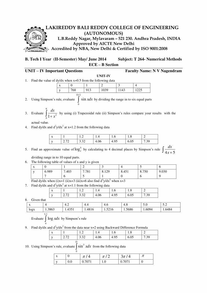
UNIT-IV
1. Find the value of dy/dx when x=0.5 from the following data
x 0 1 2 3 4
y 768 913 1039 1143 1225
2. Using Simpson’s rule, evaluate /2
0
sin xdx
by dividing the range in to six equal parts
3. Evaluate
6
2
01
dx
x by using (i) Trapezoidal rule (ii) Simpson’s rules compare your results with the
actual value.
4. Find dy/dx and d2y/dx
2 at x=1.2 from the following data
x 1 1.2 1.4 1.6 1.8 2
y 2.72 3.32 4.06 4.95 6.05 7.39
5. Find an approximate value of5loge
by calculating to 4 decimal places by Simpson’s rule 4 5
dx
x
dividing range in to 10 equal parts.
6. The following table of values of x and y is given
x 0 1 2 3 4 5 6
y 6.989
7
7.403
6
7.781
5
8.129
1
8.451
0
8.750
6
9.030
9
Find dy/dx when (i)x=1 (ii)x=3 (iii)x=6 also find d2y/dx
2 when x=3
7. Find dy/dx and d2y/dx
2 at x=1.1 from the following data
x 1 1.2 1.4 1.6 1.8 2
y 2.72 3.32 4.06 4.95 6.05 7.39
8. Given that
x 4 4.2 4.4 4.6 4.8 5.0 5.2
logx 1.3863 1.4351 1.4816 1.5216 1.5686 1.6094 1.6484
Evaluate
5.2
4
log xdx by Simpson’s rule
9. Find dy/dx and d2y/dx
2 from the data near x=2 using Backward Difference Formula
x 1 1.2 1.4 1.6 1.8 2
y 2.72 3.32 4.06 4.95 6.05 7.39
10. Using Simpson’s rule, evaluate 3
0
sin xdx
from the following data
x 0 / 4 / 2 3 / 4
y 0.0 0.7071 1.0 0.7071 0
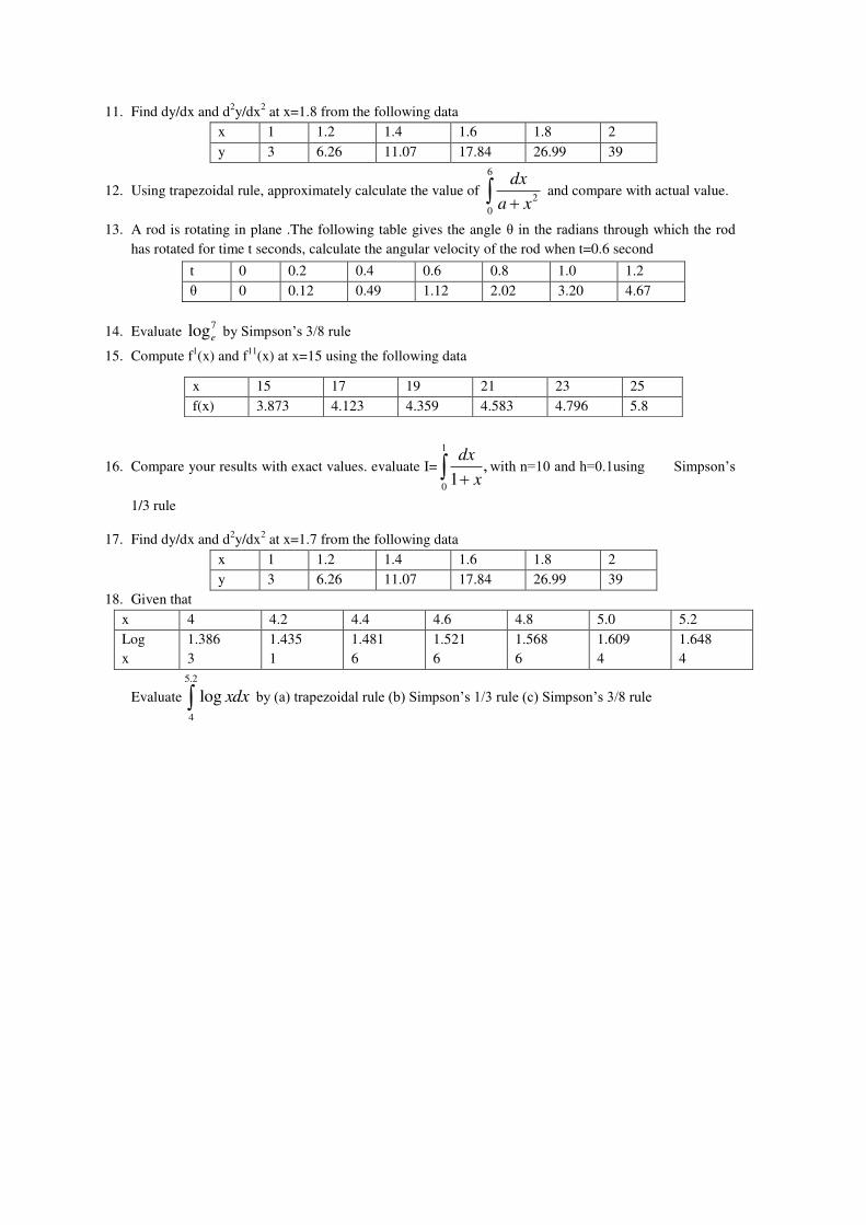
11. Find dy/dx and d2y/dx
2 at x=1.8 from the following data
x 1 1.2 1.4 1.6 1.8 2
y 3 6.26 11.07 17.84 26.99 39
12. Using trapezoidal rule, approximately calculate the value of
6
2
0
dx
a x and compare with actual value.
13. A rod is rotating in plane .The following table gives the angle θ in the radians through which the rod has rotated for time t seconds, calculate the angular velocity of the rod when t=0.6 second
14. Evaluate 7loge
by Simpson’s 3/8 rule
15. Compute f1(x) and f
11(x) at x=15 using the following data
16. Compare your results with exact values. evaluate I= ,1
1
0
x
dxwith n=10 and h=0.1using Simpson’s
1/3 rule
17. Find dy/dx and d2y/dx
2 at x=1.7 from the following data
x 1 1.2 1.4 1.6 1.8 2
y 3 6.26 11.07 17.84 26.99 39
18. Given that
x 4 4.2 4.4 4.6 4.8 5.0 5.2
Log
x
1.386
3
1.435
1
1.481
6
1.521
6
1.568
6
1.609
4
1.648
4
Evaluate
5.2
4
log xdx by (a) trapezoidal rule (b) Simpson’s 1/3 rule (c) Simpson’s 3/8 rule
t 0 0.2 0.4 0.6 0.8 1.0 1.2
θ 0 0.12 0.49 1.12 2.02 3.20 4.67
x 15 17 19 21 23 25
f(x) 3.873 4.123 4.359 4.583 4.796 5.8
LAKIREDDY BALI REDDY COLLEGE OF ENGINEERING (AUTONOMOUS)
L.B.Reddy Nagar, Mylavaram – 521 230. Andhra Pradesh, INDIA
Approved by AICTE New Delhi Accredited by NBA, New Delhi & Certified by ISO 9001:2008
B. Tech I Year (II-Semester) May/ June 2014 Subject: T 264- Numerical Methods
ECE – B Section
UNIT – V Important Questios Faculty Name: N V Nagendram
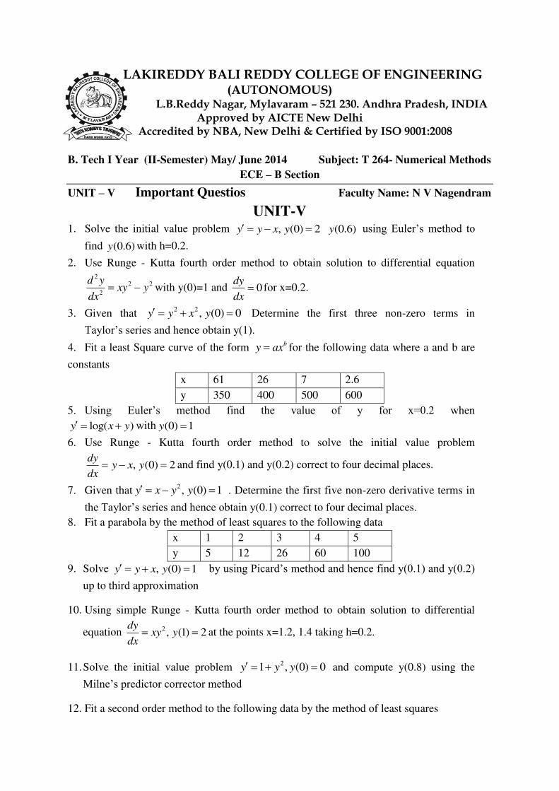
UNIT-V 1. Solve the initial value problem , (0) 2 (0.6)y y x y y using Euler’s method to
find (0.6)y with h=0.2.
2. Use Runge - Kutta fourth order method to obtain solution to differential equation 2
2 2
2
d yxy y
dx with y(0)=1 and 0
dy
dx for x=0.2.
3. Given that 2 2 , (0) 0y y x y Determine the first three non-zero terms in
Taylor’s series and hence obtain y(1). 4. Fit a least Square curve of the form
by ax for the following data where a and b are
constants
x 61 26 7 2.6
y 350 400 500 600
5. Using Euler’s method find the value of y for x=0.2 when log( )y x y with (0) 1y
6. Use Runge - Kutta fourth order method to solve the initial value problem
, (0) 2dy
y x ydx
and find y(0.1) and y(0.2) correct to four decimal places.
7. Given that2 , (0) 1y x y y . Determine the first five non-zero derivative terms in
the Taylor’s series and hence obtain y(0.1) correct to four decimal places.
8. Fit a parabola by the method of least squares to the following data
x 1 2 3 4 5
y 5 12 26 60 100
9. Solve , (0) 1y y x y by using Picard’s method and hence find y(0.1) and y(0.2) up to third approximation
10. Using simple Runge - Kutta fourth order method to obtain solution to differential
equation 2 , (1) 2dy
xy ydx
at the points x=1.2, 1.4 taking h=0.2.
11. Solve the initial value problem 21 , (0) 0y y y and compute y(0.8) using the
Milne’s predictor corrector method
12. Fit a second order method to the following data by the method of least squares
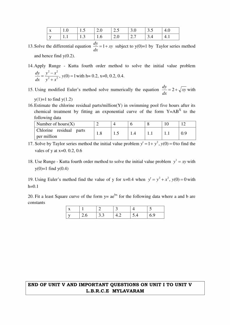
x 1.0 1.5 2.0 2.5 3.0 3.5 4.0
y 1.1 1.3 1.6 2.0 2.7 3.4 4.1
13. Solve the differential equation xydx
dy1 subject to y(0)=1 by Taylor series method
and hence find y(0.2).
14. Apply Runge - Kutta fourth order method to solve the initial value problem 2 2
2 2, (0) 1
dy y xy
dx y x
with h= 0.2, x=0, 0.2, 0.4.
15. Using modified Euler’s method solve numerically the equation xydx
dy 2 with
y(1)=1 to find y(1.2)
16. Estimate the chlorine residual parts/million(Y) in swimming pool five hours after its
chemical treatment by fitting an exponential curve of the form Y=ABX
to the
following data
Number of hours(X) 2 4 6 8 10 12
Chlorine residual parts
per million 1.8 1.5 1.4 1.1 1.1 0.9
17. Solve by Taylor series method the initial value problem21 , (0) 0y y y to find the
vales of y at x=0. 0.2, 0.6
18. Use Runge - Kutta fourth order method to solve the initial value problem xyy 1with
y(0)=1 find y(0.4)
19. Using Euler’s method find the value of y for x=0.4 when 2 2 , (0) 0y y x y with
h=0.1
20. Fit a least Square curve of the form y= aebx
for the following data where a and b are
constants
x 1 2 3 4 5
y 2.6 3.3 4.2 5.4 6.9
END OF UNIT V AND IMPORTANT QUESTIONS ON UNIT I TO UNIT V
L.B.R.C.E MYLAVARAM