numerical stability and control analysis towards falling ... · pdf filenumerical stability...
TRANSCRIPT

N ASA / CR-1998-208730
Numerical Stability and Control Analysis
Towards Falling-Leaf Prediction
Capabilities of Splitflow for Two Generic
High-Performance Aircraft Models
Eric F. Charlton
Lockheed-Martin Tactical Aircraft Systems, Fort Worth, Texas
National Aeronautics and
Space Administration
Langley Research CenterHampton, Virginia 23681-2199
September 1998
Prepared for Langley Research Centerunder Contract NAS1-96014
https://ntrs.nasa.gov/search.jsp?R=19990008181 2018-04-18T12:19:32+00:00Z

Available from:
NASA Center for AeroSpace Information (CASI)7121 Standard Drive
Hanover, MD 21076-1320
(301) 621-0390
National Technical Information Service (NTIS)
5285 Port Royal Road
Springfield, VA 22161-2171
(703) 605-6000

Numerical Stability and Control Analysis Towards
Falling-Leaf Prediction Capabilities of Splitflow for Two
Generic High-Performance Aircraft Models
Eric E Charlton
Lockheed Martin
Tactical Aircraft Systems
Abstract
Aerodynamic analyses are performed using the Lockheed Martin Tactical Aircraft Systems
(LMTAS) SpliO'tow computational fluid dynamics code to investigate the computational predic-
tion capabilities for vortex-dominated flow fields of two different tailless aircraft models at large
angles of attack and sideslip. These computations are performed with the goal of providing use-ful stability and control data to designers of high-performance aircraft. Appropriate metrics for
accuracy, time, and ease of use are determined in consultation with both the LMTAS Advanced
Design and Stability and Controls groups. Results are obtained and compared to wind tunneldata for all six forces and moments. Moment data is combined to form a "falling leaf" stability
analysis. Finally, a handful of viscous simulations were also performed to further investigate
nonlinearities and possible viscous effects in the differences between the accumulated inviscid
computational and experimental data.
Contents
1 Nomenclature 4
2 Introduction 6
3 Configuration 6
4 Computational Resources 74.1 Inviscid ........................................ 8
4.2 Viscous ........................................ 9
5 Metrics 9
5.1 Advanced Design Metrics ............................... 95.2 S&C Metrics ..................................... 10
5.3 Runtime ........................................ 11
6 Results
6.1 MTVI
6.1.1
6.1.2
6.2 ICE
6.2.1
6.2.2
6.2.3
6.2.4
6.2.5
• • ° ° • • * • ° ° ..... ° • * • • ° ....... • • • . ° ........
MTVI Results,/3 = 0 ° ............................
MTVI Results, B = 2° ............................
• • • , . . ° • • * ........ , ..... * .... • . • . * ........
Tailless Delta (ICE) Results: fl = 0° .....................
Tailless Delta (ICE) Results: fl = 5° .....................
Tailless Delta (ICE) Results: B = 10 ° ....................
Tailless Delta (ICE) Results: _ = 20 ° ...................
Tailless Delta (ICE) Results, B-sweep, a = 20 ° ..............
6.3 Highlights .......................................
6.4 Improvements .....................................
6.5 Solution Adaption ...................................
6.6 Leading Edge Resolution ...............................
6.7 Convergence .....................................
6.8 Grid Convergence ..................................
6.9 CPU Requirements .................................
11
12
13
16
18
19
22
25
28
31
34
34
38
38
40
40
43
8 Conclusions 49
8.1 Future Efforts ..................................... 49
9 Acknowledgments 52
References 53
7 Failing-Leaf Phenomenon 44

List of Figures
1 Baseline aircraft model configurations ........................ 6
2 Omnigrid and near-surface prismatic grid example on the body symmetry plane . . 8
3 Improved M v results for the ICE configuration ................... 364 ICE model pitch moment rotary balance test data .................. 37
5 Effect of different solution adaption parameters on computed vortex structure . . . 39
6 Leading edge resolution for the ICE model ...................... 40
7 Force/moment convergence, Tailless Delta Wing, Moo = 0.3, a = 15°,/3 = 5 ° . . 41
8 Force/moment "convergence" Tailless Delta Wing, Moo -- 0.3, a : 30 °,/3 = 20 ° . 41
9 Grid converence study, ICE model, a -- 24 °,/3 : 10 ° . ............... 42
10 Contour plot of Cp difference, ICE model at a -- 24 °,/3 = 10° ........... 43
11 Falling leaf motion .................................. 44
12 Falling leaf susceptibility region ........................... 45
13 Falling leaf results,/3 ----10° ............................. 46
14 Falling leaf results,/3 = 20° ............................. 47
15 Falling leaf results, MTVI,/3 : 2° .......................... 48
16 New grid generation method ............................. 51
List of Tables
1
2
3
4
5
MTVI a//3-sweep (inviscid) ............................. 7
Tailless Delta (ICE) a-sweep (inviscid) ....................... 7
Tailless Delta (ICE)/3-sweep (inviscid) ....................... 7
Tailless Delta (ICE), viscous ............................. 8
ICE prismatic grid parameters ............................ 9

1 Nomenclature
Parameters:
a angle of attack, usually in degrees.
sideslip angle, usually in degrees.
A wing sweep angle, usually in degrees.
t/c wing thickness to chord ratio, usually in percent.
Variables:
C_ lateral stability derivative, OCl/O/3 (Section 7).
Cn_ directional stability derivative, OCn/O/3 (Section 7).
CnaDYN Dutch-roll stability parameter (Section 7).
F_, by, Fz force coefficients in the body x-, g-, and z-axis respectively, also referred to as CA,
Cy, and CN respectively.
Ixx, Izz, lzz moments of inertia about the x-, z-, and z/z axes respectively.
Mx, M u, M_ moment coefficients around the body x-, y-, and z-axis respectively, also referred to
as Cl, Cm, Cn or CLLB, CLM, CLNB ("C little L body," "C little M," and "C little N body,"where "body" refers to the reference axis).
SRYP synchronous roll-yaw parameter (Section 7).
velocity, (u, v, w) in body axes.
vorticity (V x v-'),in body axes.
Abbreviations:
BC boundary condition
CFD computational fluid dynamics
ICE LMTAS Innovative Control Effectors (tailless delta wing) model
LE leading edge
LaRC NASA Langley Research Center
LM Lockheed Martin
LMTAS Lockheed Martin, Tactical Aircraft Systems division
MTVI NASA Langley Modular Transonic Vortex Interaction air_ raft model
PVM Parallel Virtual Machine library
RCS radar cross section
4

SARL SubsonicAerodynamicResearchLaboratory
S&C stabilityandcontrols
WT windtunnel(in thisreport,usuallySARL)

(a) MTV1 (b) ICE
Figure 1: Baseline aircraft model configurations
2 Introduction
Aerodynamic design of high-performance aircraft requires detailed knowledge of the often-com-
plicated airflow around the surface. High-performance aircraft usually make use of chines and
surface blends between fuselages and wings to encourage vortex lift for maneuvering without sharp
intersections between the wing and fuselage. Recent concerns regarding radar cross section (RCS,
i.e. "stealth") have placed additional emphasis on sharp, well-defined surface intersections and are
often leading to tailless aircraft designs.
The use of modified delta wings and sharp-edged leading edges often leads to vortex-dominated
flows. The problem is further complicated by the large ranges of angle of attack (or) and sideslip (fl)
commonly experienced by tactical aircraft. The blended fuselage or chine along with the leading
edge of the wing often creates multiple vortices which interact in complicated and highly-nonlinearmanners.
The present study is part of the NASA Langley Research Ce lter sponsored project (described
in References 1-8) aimed at assessing the viability of using verious state-of-the-art CFD Euler
technology for efficient application of aerodynamic analysis during the preliminary design process.
This work demonstrates how the LMTAS-developed Cartesian/unstructured grid method, the Split-
flow code, can be used to rapidly analyze the flow around high-performance aircraft shapes and
advance their design process. Results for the test cases are presented and measured with respect
to runtime, accuracy, and the ease of use. In order for CFD to be used routinely in the design of
high-performance aircraft, certain standards must be met for acc Jracy, time required, and ease ofuse.
3 Configuration
Two configurations were analyzed to provide comparison data Ibr different types of aircraft, as
shown in Figure 1. Each is a tailless delta wing aircraft model, 3ut a different method is used in
each to blend the wing and fuselage. In both cases, the flows are dominated by multiple interacting

/30
2
Ol
I °16 12 16 20 25 1301L40130 35 40 45
Table 1: MTVI c_//3-sweep (inviscid)
0 0 10 15 20 30
5 0 10 15 20 30
10 0 5 10 15 20 22 24 26 28 30
20 0 5 10 15 20 22 24 26 28 30
Table 2: Tailless Delta (ICE) a-sweep (inviscid)
vortices. As these vortices interact, their influence on each other and the upper surface of the wing
will set the corresponding aerodynamic performance of the vehicles. In each case, the key to a
vortex-driven solution is resolving the vortex core. But adaption to the core can be tricky--at high
a, vortex breakdown can become an important effect, and vortex breakdown is especially aggravated
by high/3.
The first configuration is the NASA Langley Modular Transonic Vortex Interaction (MTVI)
model. MTVI is a delta wing with a long chined fuselage, as shown in Figure l(a). At high o_,
vortices are created off of both the chine and the leading edge of the wing which interact as they
pass over the upper surface of the aircraft model. The geometry and wind tunnel forces and moment
data were provided by NASA Langley Research Center [9]. The MTVI cases computed are listedin Table 1.
The second configuration is the LMTAS tailless delta wing, referred to here (and in many ear-
lier publications) as the Innovative Control Effectors (ICE) model. The ICE model has a blended
fuselage and canopy, with a serrated ("broken") trailing edge. The ICE model also has very high
camber with a very thin wing airfoil (t/c = 4%), which caused difficulty during the grid generation
phase as will be discussed later in Section 5.3. The ICE model is shown in Figure l(b). Table 2
lists the cases performed for the sweeps across angle-of-attack, Table 3 lists the additional cases
performed for the sweep across slip angle, and Table 4 lists the viscous cases that were added to
investigate the possibility of viscous effects causing discrepancies between the inviscid solutions
and the Subsonic Aerodynamic Research Laboratory (SARL) wind tunnel data.
4 Computational Resources
Two versions of the Lockheed Martin unstructured Cartesian code Spli_ow were used for this anal-
ysis. The newer code, Omnigrid Spli_ow, is a parallel code using Parallel Virtual Machine (PVM,
z5 I5.0 /3 20.0[7.5110.0112.5115.0117.5 I
Table 3: Tailless Delta (ICE)/3-sweep (inviscid)

10 22 I 24 28
20 22 I 28
Table 4: Tailless Delta (ICE), visc,_us
_-55
(a) Slice throughan omnigrid (b) Slice through a hybrid grid
Figure 2: Omnigrid and near-surface prismatic grid example on the body symmetry plane
described in [10]) that solves the Euler equations. Hybrid Splitflow is a vector code that was used to
solve the Navier-Stokes equations. The parallel Omnigrid cases w ere computed on networks of SGI
workstations, an HP 2000-series supercomputel; and LMTAS Crav J-90's. The vector computations
were performed on the Cray J-90's. An example of an omnitree grid and the prismatic layer near
the surface of a hybrid grid are shown in Figures 2(a) and 2(b) respectively.
Each version of Split]tow uses a tree-based data structure to build and store the grid. Compu-
tational grids are built by starting from a "root" cell and recursively refining one cell into smaller
"children" grid cells. Ornnigrid Splitflow yields additional efficiency by refining grid cells in each
direction independently, yielding as few as two cells per cell refinement; the octree model used by
Hybrid Spli(flow yields a constant eight-children-per-parent cell re finement. Each code uses a finite-
volume conservation scheme with an upwind flux formulation and has a preconditioner available forlow Mach number flow solutions.
4.1 Inviscid
The inviscid simulations were computed with Omnigrid Splioqo.. In practice, the directional cell
splitting used by Omnigrid SpliO'tow can yield the same grid res, flution as Hybrid Splioqow using
approximately half the number of cells. Omnigrid SpliOqow uses a pointwise semi-implicit time
update with subiterations for more-efficient parallel computation.

Numberof layersGrowthrateInitialspacing
91.1
0.001
Table5: ICE prismatic grid parameters
4.2 Viscous
The five viscous simulations were computed with Hybrid SpliO'tow. Hybrid Spli_tow uses a pris-
matic grid grown from the surface in addition to the Cartesian octree grid. The prismatic grid is
sized according to an approximate flat plate boundary layer for the aircraft's flight conditions. For
the ICE model and the flight conditions of interest (Re = 1.9 × 10⁶/ft, Moo = 0.3), the prismatic
grid parameters are listed in Table 5.
Hybrid Spli_ow uses a two-equation turbulence model for accurate solution of turbulent viscous
flow fields. The k-kl and k-l models developed at LMTAS are comparable in accuracy to the k-c
and k-_v turbulence models, but they do not require nearly as fine near-wall grid spacing as do those
models [11, 12]. In addition, unique and consistent wall function boundary conditions have been
developed for the k-kl and k-l turbulence models.
For this study, the k-kl model was used without the wall function boundary condition. The vis-
cous sublayer and buffer regions of the turbulent boundary layer are within the prismatic grid. The
model has been validated for both attached and separated turbulent flows. Unlike the k-, model,
no ad-hoc corrections are required at separation and reattachment points to obtain reasonable solu-
tions. The k-kl model has been applied extensively to a wide variety of aerospace flows and has
been shown to be robust and comparable in accuracy to other well calibrated two equation turbu-
lence models [12, 13].
5 Metrics
In order to measure LMTAS aerodynamic capabilities with regards to its users in Advanced Design
and Stability and Controls, metrics were produced in consultation with these groups at LMTAS.
The metrics discussions focused on time, accuracy, and ease of use. The metrics presented in this
report represent a combination of both what is needed and what is wanted. While these metrics are
not necessarily met in the present study, such discussion to establish the desired parameters can be
very useful in tool development.
5.1 Advanced Design Metrics
The Advanced Design group is mostly concerned with computing aerodynamic properties around
multiple cruise and maneuver points. For their applications, one polar is not enough, but the number
of polars depends on the configurations under study. Usually extra data points are necessary to
determine the effect of deployed high-lift devices and to build a database of trim data.
An ordinary aerodynamic simulation schedule would require at least three trailing-edge flap
settings, three tail deflections, and three leading-edge flap settings, resulting in approximately 27
polars. To be most useful, Advanced Design would like the results of a full matrix in 24 hours;
ideally then CFD techniques are expected to be able to finish approximately one polar per hour.
The Advanced Design group's current analysis techniques are not as fast at LMTAS, however--it
takes about one week to do a complete analysis. The current analysis codes used run quickly, but
eachrequiressignificantsetupandpost-processingtime.However,if CFDweretoreachthesameturnaroundtimeasthecurrentmethod,it will becometheprelirrinaryaerodynamicdesigntoolofchoice.
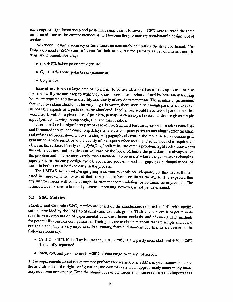
AdvancedDesign'saccuracycriteriafocusonaccuratelycomputingthedragcoefficient,Co.
Drag increments (ACt9) are sufficient for their needs, but the l:fimary values of interest are lift,
drag, and moment. For drag:
• CD -4- 5% below polar break (cruise)
• Co ± 10% above polar break (maneuver)
• CDo+5%
Ease of use is also a large area of concern. To be useful, a tool has to be easy to use, or else
the users will gravitate back to what they know. Ease is somewhat defined by how many training
hours are required and the availability and clarity of any documentation. The number of parameters
that need tweaking should not be very large; however, there should be enough parameters to cover
all possible aspects of a problem being simulated. Ideally, one would have sets of parameters that
would work well for a given class of problem, perhaps with an expert system to choose given simple
input (perhaps (_, wing sweep angle, t/c, and aspect ratio).
User interface is a significant part of ease of use. Standard Fortran-type inputs, such as namelists
and formatted inputs, can cause long delays where the computer gives no meaningful error message
and refuses to proceed----often over a simple typographical error in the input. Also, automatic grid
generation is very sensitive to the quality of the input surface mesh, and some method is required to
clean up the surface. Finally using Splitflow, "split cells" are often a problem. Split cells occur where
the cell is cut into multiple disjoint volumes by the body. Refining the grid does not always solve
the problem and may be more costly than allowable. To be useful where the geometry is changing
rapidly (as in the early design cycle), geometric problems such as gaps, poor triangulations, or
too-thin bodies must be fixed early in the process.
The LMTAS Advanced Design group's current methods are _equate, but they are still inter-
ested in improvements. Most of their methods are based on lin._ar theory, so it is expected that
any improvements will come through the proper accommodation ."ornonlinear aerodynamics. The
required level of theoretical and geometric modeling, however, is _mt yet determined.
5.2 S&C Metrics
Stability and Controls (S&C) metrics are based on the conclusions reported in [14], with modifi-
cations provided by the LMTAS Stability and Controls group. Tl:_.eirkey concern is to get reliable
data from a combination of experimental databases, linear meth¢ ds, and advanced CFD methods
for potentially complex configurations. Their goals are to obtain methods that are simple and quick,
but again accuracy is very important. In summary, force and mommt coefficients are needed to the
following accuracy:
• CL -1- 5 _ 10% if the flow is attached, +10 _ 20% if it is partly separated, and +20 ,,0 30%
if it is fully separated.
• Pitch, roll, and yaw-moments +20% of data range, within 2' of zeroes.
These requirements do not cover trim nor performance restrictions. S&C analysis assumes that once
the aircraft is near the right configuration, the control system can appropriately counter any unan-
ticipated force or response. Even the magnitudes of the forces and moments are not so important as
l0
thesigns,i.e.thesystemneedstoknowwhichwaytopush,butit isassumedthatthecontrolsystemhassufficientforcetoaccomplishthetask.(Whilethisis theassumption,it iscriticaltoknowthatagivendeflectionincontrolsurfacewill producecorrectdirectionof forceandmoments--thiscouldbeaparticularproblemwithphenomenonsuchasaileronreversal.)
5.3 Runtime
Since Splio'tow was intended to be an automatic grid generator and flow solver, the setup time for
Splioqow is minimal. Once the CAD surface cleanup is complete, one configuration setup usually
works for all of the runs. The computations, however, took much longer than anticipated.
Reruns were often required, often to compensate for thin-wing based split cell problems on the
ICE configuration. There are only two known ways to deal with split cells using Splioqow:
1. reduce dxyzmin allowing cells to be cut smaller than the body thickness, so each side is
properly handled.
2. or zero mxdelete causing no grid coarsening with grid adaption, and reducing the chances
of producing a split cell.
Both of these values are described in [15]. Decisions regarding their use fall to the user's discretion.
Boundary condition and turbulence models also caused some difficulty. In particular, when
attempting to use a (less expensive) slip BC on the sting, the turbulence model would failand crash
the code. Finally, The Omnigrid Splitflow flow solver appears to be considerably less efficient than
the older Hybrid-Spli_low code, and this greatly affected turnaround, as discussed in more detail inSection 6.9.
6 Results
Results for this analysis are presented according to the following list. Individual plots are included
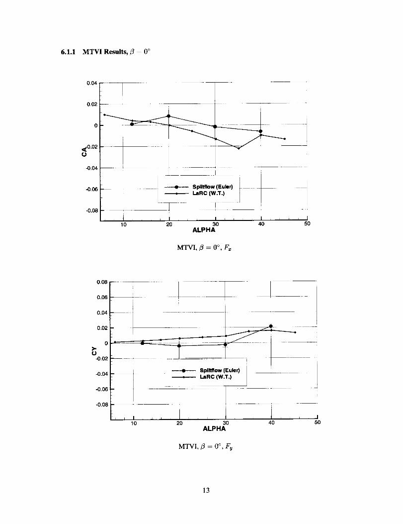
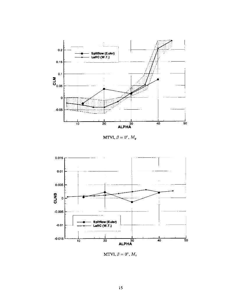
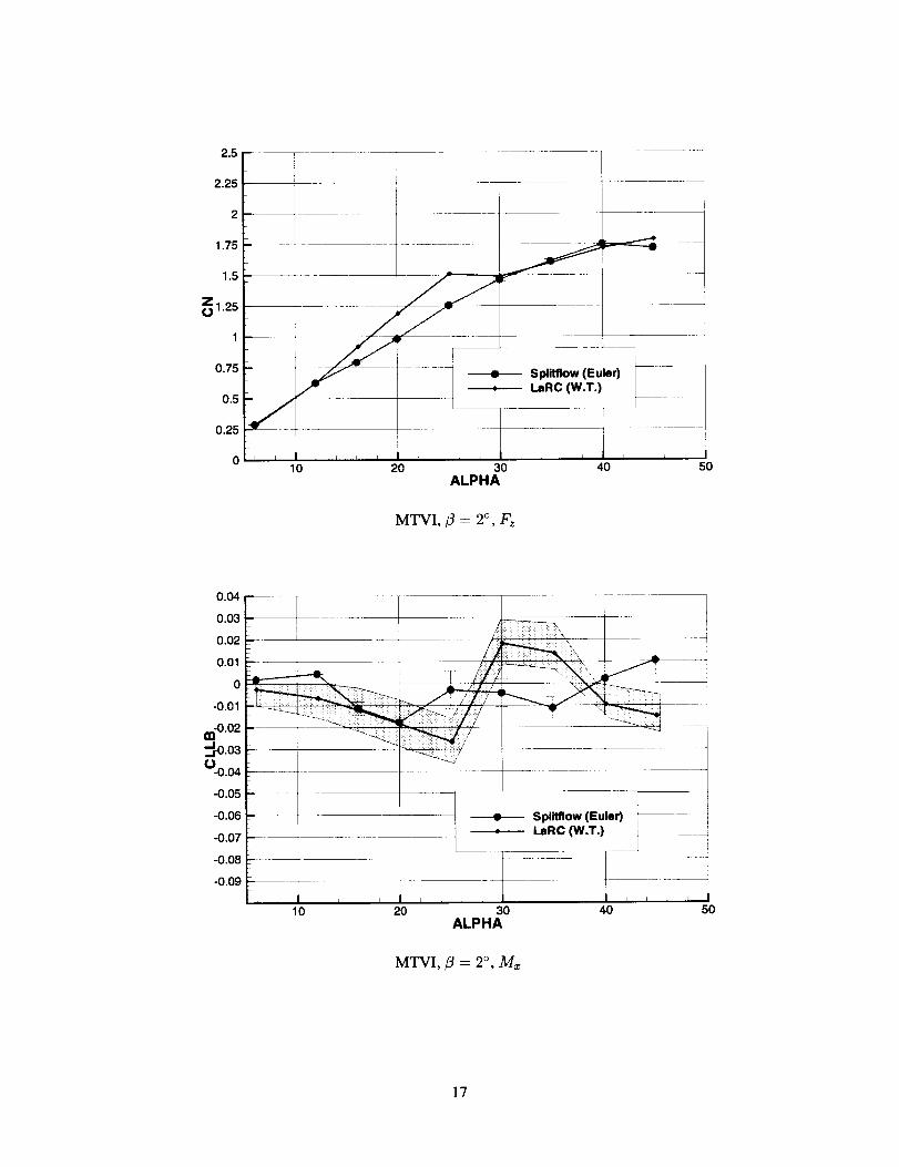
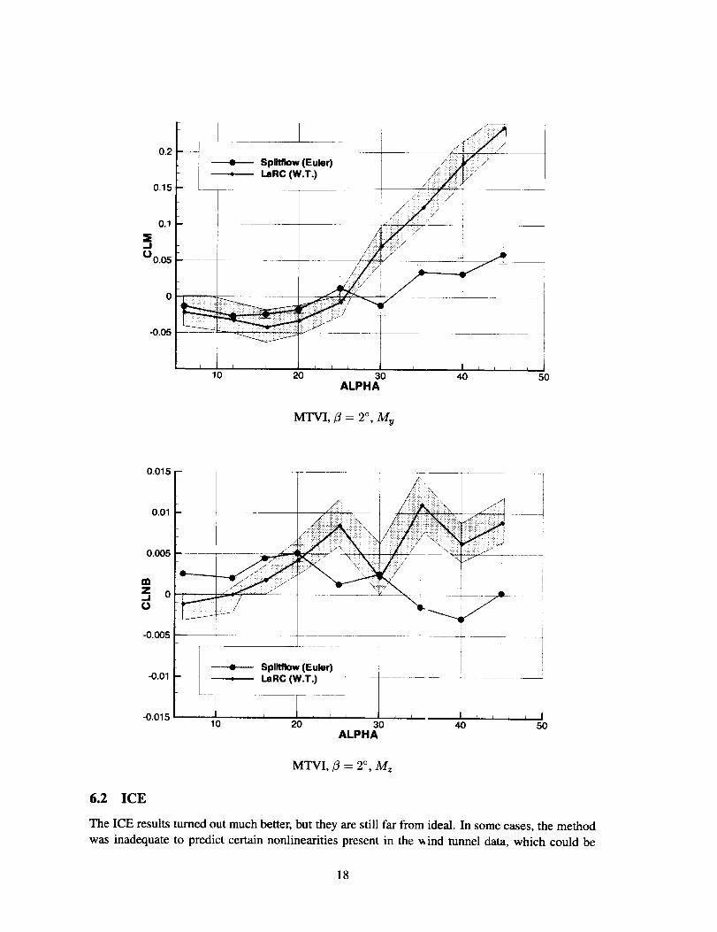
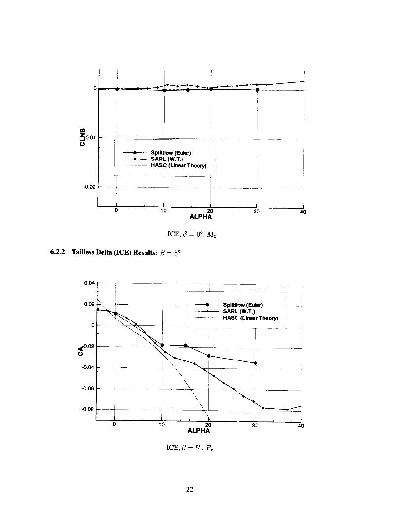
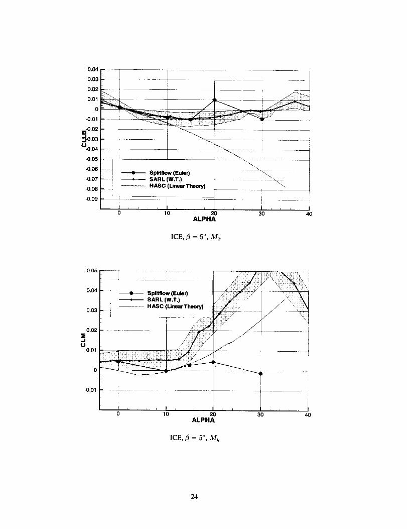
in Sections 6.1 and 6.2 for the MTVI and ICE configurations, respectively. For each data set, six
plots are included, for the body-axis forces (Fx, F_, and Fz) and body-axis moments (Mx, My, and
Mz), in that order.
• MTVI, a-sweep
-_=0 o
__=2 o
• Tailless Delta (ICE), a-sweep
-/3=0 °
_3=5 °
- _ = 10°
- _ = 20°
• Tailless Delta (ICE),/3-sweep
11
Thecoefficientsof interest are:
• Fx, Fu, Fz force coefficients in the x-, y-, and z-directions (body axis) respectively.
• M_, Mu, Mz moment coefficients about the z-, y-, and z-directions (body axis) respectively,
also referred to as Ct, Cm, Cn and CLLB, CLM, CLNB.
The MTVI runs performed are listed in Table 1, while the ICE runs are listed in Tables 2,
3, and 4 for the a-sweeps, B-sweep, and viscous series respectively. The chosen test matrix for
these cases covers a wide variety of angles of attack and sideslip for the two similar configurations,
MTVI and ICE. While expanding the range of either variable (particularly sideslip for falling-leaf
predictions) would be helpful, a lot has been learned regarding how to analyze cases such as this and
where some of the potential pitfalls lie. As expected, the use of the Euler equations as a physical
basis improved the prediction capability for nonlinear phenomenon. Although not reported here,
as expected, nonlinear phenomenon related to viscous effects (vortex breakdown, separation andreattachment, etc.) were not predicted well.
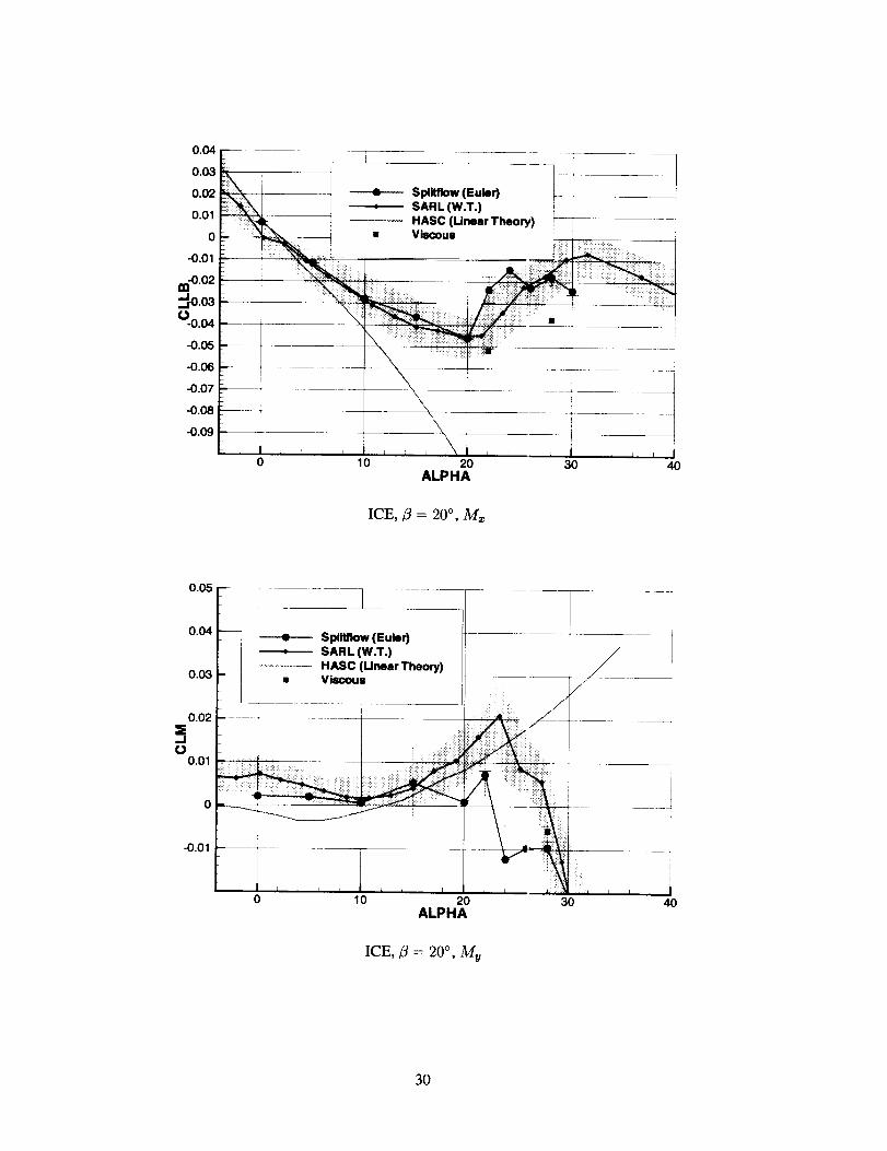
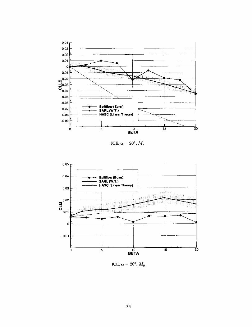
The "acceptable prediction ranges" (grey areas) on the moment coefficient plots in Sections 6.1and 6.2 are based on the S&C criteria discussed in Section 5.2. Since the focus is on moment
coefficients at nonzero B, only those are specifically shown on the included plots. Here, a tighter
tolerance of only +10% is used to better demonstrate areas of success and desired improvement--
+20% of the data range is 40% of the data range, as specified by the S&C criteria, or nearly half the
plotted area. These regions are hand-drawn on underlays for the plots using Tecplot [16], and they
represent an approximate (not numeric) region of acceptability. The computed results also contain
"error bars" which show the fluctuation in force or moment coefficient over (approximately) thelast 100 iterations.
The linear theory results are produced by the HASC code [17]. HASC uses linear theory models
modified through experience at analyzing high-performance aircraft.
6.1 MTVI
The MTVI results did not turn out as well as expected. While some of the nonlinear breaks were
captured near the correct a, the magnitudes were often significantly different than the wind-tunnel
data. Part of the problem is the wide range of angle of attack, 0 < a < 45 °. At large a, much ofthe flow is separated into complex vortical flows, and in some instances vortex breakdown causes
unsteady flows that are difficult to simulate even with Navier-Stol es methods.
12
6.1.1 MTVI Results,/3 : 0 °
0.04 F
0.02
_-0,02O
-0.04
-0.06
-0.08
Splitflow (Euler)
I.aRC (W.T.)
i i i _ L i i L J J i i i i ; i
10 20 30
ALPHA
I I i I
40 50
MTVI,/3 = 0°,Fx
Splitflow (Euler)
I.aRC (W.T.)
10 20 30ALPHA
MTVI,/3 = 0 °, Fu
4O 50
13

Zl.25
1 I -
0.75
0.25
010
S plit'flow (Euler)LaRC (W.T.)
20 30 40 50ALPHA
MTVI,/3 = 0 °, Fz
0.04
0.03
0.02
0.01
0
-0.01
nn-O.02
_.0.03
0-0.04
-0.05
-0.06
-0.07
-0.08
I
! ] ],
-0.09
20 30 40 50ALPHA
MTVI,/3 = 0°, Mz
14
0.2
0.15
0.1
=E.=1
¢') 0.05
-0.05
Splltflow (Euler)I.aRC (W.T.)
10 20 30 40 50ALPHA
MTVI, fl = 0°, My
0.015
0.01
0.005
mz 0Jo
-0.01----e--- Splitflow (Euler)
i
I.aRC (W.T.)l
10 20 30ALPHA
40 50
MTVI, g -- 0 °, Mz
15

6.1.2 MTVI Results,/3 = 2°
0.04
0.02
, I
3OALPHA
50
MTVI,/3 = 2°, Fx
0.08
0.06
0.04
0.02
0>-
-0.02
-0.04
-0.06
-0.08 --r- ....
, i i
10 20
Splitflow (Euler) ....I.aRC (W.T.)
I i I L
3OALPHA
\
IIIli
4O 5O
MTVI,/3 : 2°, F_
16
2.5
2.25
2
1.75
1.5
Zl.25
1
0.75
0.5
0.25
0
+ Splitflow (Euler)LaRC (W.T.)
10 20 30ALPHA
4O 5O
MTVI,/3 = 2 °, Fz
0.04
0.03
i
+ Splitflow (Euler)--_----- LaRC (W.T.)
10 20 30 40 50ALPHA
MTVI,/3 = 2°, Mz
17
0.15
0.1
:EJ
00.05
!I
Splitfk)w (Euler) ILaRC (W.T.) !
10 20 30 40 50ALPHA
MTVI, _ = 2°,M_
0.015
0.01
0.005
-0.015
-----e---- Splltflow (Euler)LaRC (W.T.)
10 20 30 40 50ALPHA
MTVI,/3 = 2 °, Mz
6.2 ICE
The ICE results turned out much better, but they are still far from ideal. In some cases, the method
was inadequate to predict certain nonlinearities present in the v, ind tunnel data, which could be
18

attributed to the inherent limitations of the the Euler equations. The Navier Stokes solutions were
somewhat better. Perhaps a thicker prismatic grid, or a smoother transition from the prismatic grid
to the Cartesian grid, would have improved them.
6.2.1 Tailless Delta (ICE) Results:/3 : 0 °
0.02
-0.04
._. A
- ----e---- Splifflow (Euler)SARL (W.T.)HASC (Linear Theory)
\\
10 20 30ALPHA
40
ICE,/3 = 0 °, Fz
19

0.04
-0.02
>-0
-0.04
-0.06
-0.08
I
----e---- Splitflow (Euler)SARL (W.T.)
........... HASC (Linear Theory)
I
10 20ALPHA
3O
ICE, j3 = 0 °, F v
4o
1.2
1.1
1
0.9
0.8
0.7
0.6
Z 0.50
0.4
0.3
0.2
0.1
0
-0,1
¢ Split,low (Euler). SARL (W.T.)
HASC (Linear Theory)
10 2OALPHA
I I30 40
ICE, 3 -- 0 °, Fz
2O

0.04
0.03
0.02
0.01
0
-0.01
1:0-0.02
_r0.03
t_.0.04
-0.05
-0.06
-0.07
-0.08
-0,09
---e--- Splitflow (Euler)SARL (WT)HASC (Unear Theory)
i i I i I0 10 20
ALPHA
J ; J I
30I I I I
4O
ICE, fl = 0°, M=
0.05
0.04
0.03
0.02=E-IO
0.01
-0.01
¢ Splitflow (Euler). SARL (WT)
HASC (Linear Theory)
10 20ALPHA
ICE,/3 = 0 °, Mu
30 40
21
m
0.01
-0.02
Spl_ (Euler)SARL (W.T.)HASC (Linear Theory)
J
7
10 20ALPHA
ICE, B = 0°, M,
3O
6.2.2 Tailless Delta (ICE) Results: B = 5 °
0.04
0.02
,_-0.02
-0.08
r ]
Splltflow (Euler) --_, . SARL (W.T.) =
i
HAS(: (Linear Theory) :
I li
0
\
10 20ALPHA
3O 4O
ICE, B = 5 °, Fx
22

0.04
0.02
-0.06
-0.08
----e---- Splitflow (Euler)SARL (W.T.)
............ HASC (Unear Theory)
I
10 20ALPHA
3o 4o
ICE, _ = 5°, F_
----e--- Split'flow (Euler)SARL (W.T.)HASC (Linear Theory)
0 10 20ALPHA
ICE, fl = 5°, Fz
30 4O
23
0.04
0.03
0.02ii_ r
0.01 : _
o-0.01 -
in-O.02
..,_.0.03 ----
0.0.04 __ __
-0.05
-0.06
-0.07
-0.08
-0.09
J
Splitflow (Euler)i! _ SARL (W.T.)
HASC (Unear Theory)
2OALPHA
I I I I
0 10
\_\\
ii i i i
3O 40
ICE,/3 = 5°, M=
-0.01
Splltflow (Euler)SARL (W.T.)HASC (Unear Theory)
10 20ALPHA
ICE,/3 = 5 °, Mu
3O 4O
24

m
._0.010
-0.02
SARL (W.T.)HASC (Linear Theory) 1
lI i i J I J I /
10 20ALPHA
ICE, 3 = 5°, Mz
30 4O
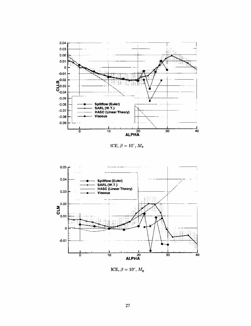
6.2.3 Tailless Delta (ICE) Results: B = 10°
0.04
0.02
-0.04
.0.06
.0.08
I i I I ; I i
0 10
_. S plitllow (Euler), SARL (W.T.)
HASC (Linear Theory)+ Viscous
20ALPHA
I I I I J L I
30 4O
ICE, fl = 10 °, Fx
25

0.04
0.02
----e---- Splitflow (Euler) -SARL (W.T.)HASC (Linear Theory)
--_---- Viscous
10 20ALPHA
ICE, _ = 10 °, Fy
3o 4o
10
e
2OALPHA
ICE, 13 -- 10 °, F_
Splifftlow (Eule oSARL (W.T.)HASC (Linear Theory)Visco =s
3O 4O
26
0.04
0.03
0.02
0.01
0
-0.01
m-o.o2__-0.03
0-0.04
-0.05
-0.06
-0.07
-0.08
-0.09
----e---- Splitltow (Euler)SARL (W.T.)
........... HASC (Linear Theory)-----e---- Viscous
I
I0 10 20
ALPHA3O 4O
ICE,/3 = 10 °, M=
0.05
0.04
0.03
0.025,,IO
0.01
_1 ......
S plitflow (Euler)SARL (W.T.)HASC (Unear Theory)Viscous .... I. f/JJ J I
-0.01
0 10 20ALPHA
ICE, ]3 = 10 °, M v
3O 4O
27

0
m
._0.010
0
Split/low (Euler)* SARL (W.T.)
HASC (Linear Theow)Viscous , \
\
30 40
ICE,/_ -- 10 °, Mz
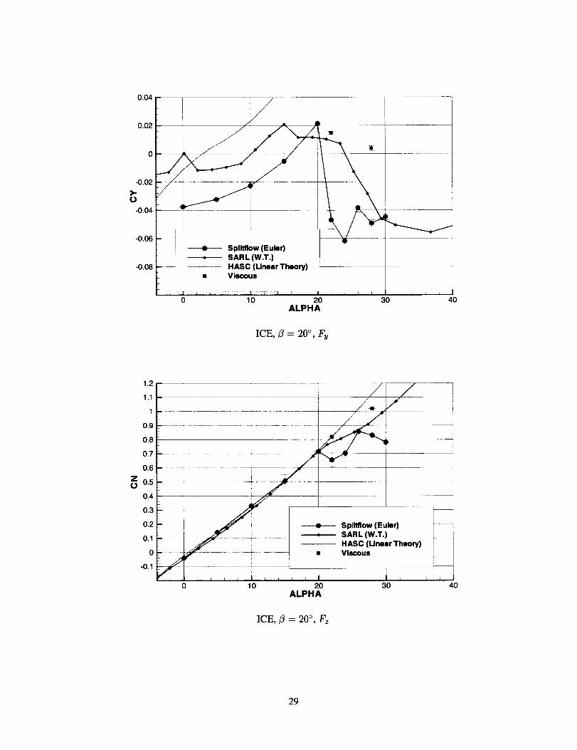
6.2.4 Tailless Delta (ICE) Results: 3 = 20°
_.0.02(J
-0.04
-0.06
0
\10 20 30 40
ALPHA
ICE,/3 = 20 °, Fx
28
0.04
0.02
----e----- Splitfiow (Euler)SARL (W.T.)HASC (Linear Theory)
• Viscous
I
10 20ALPHA
3o 4o
ICE,/3 = 20 °, Fu
0.6
Z 0.50
0.4
0.3
0.2
0.1
0
-0.1
0 10
Splitflow (Euler)SAR L (W.T.)HASC (Linear Theory)Viscous
2OALPHA
30
ICE,/3 -- 20 °, Fz
4o
29
0.04
0.03
0.02
0.01
0
-0.01
m-O.02
._,rO.03
0-0.04
-0.05
-0.06
-0.07
-0.08
-0.09
¢ Splltflow (Euler)* SARL (W.T.)
HASC (Unear Theory)Viscous
2OALPHA
1
3O 40
ICE,/3 = 20 °, M=
0.05
0.04
0.03
0.02
,-I0
0.01
+ Sp,tnow (ELder)* SARL (W.T.)
HASC (Linear Theory)• Viscous
/
-0.01
0 10 20ALPHA
30 40
ICE, 13= 20 °, My
3O

0 = Splitflow (Euler), SARL (W.T.)
HASC (Linear Theory)• Viscous
0 10 20ALPHA
\\\
3O
ICE,/3 = 20 °, Mz
4O
6.2.5 Tailless Delta (ICE) Results,/3-sweep, _ -- 20 °
S plitflow (Euler)SARL (W.T.)HASC (Linear Theory)
i i i i L
0 5 10BETA
15 20
ICE, a = 20 °, Fz
31

0.1
0.O8
0.06
0.04
0.02
>" 0 _(9
-0.02
-0.04:
-0.06
-0.08
f"J .... T /
_zJ _ _ t
. SAR L (W.T.) I
• HASC (Uneer The°w) t
5 10 15 20BETA
ICE, a -- 20°, Fu
Split/low (Euler)SARL (W.T.)HASC (Linear Theory)
5 10BETA
ICE, a = 20°, Fz
15 20
32
-----e---- Splltflow (Euler)SARL (W.T.)HASC (Linear Theory)
5 10 15BETA
ICE, a -- 20 °, M=
20
0.05
0.04
0.03
0.02=Z,J(.,1
0.01
-0.01
I I i I
i
I I I i I
i I I I I i I I
10BETA
15
ICE, a -- 20°, My
20
33
_i_iiiiiiii!iii_iiiii!iiiii!
----e---- Splitfiow (Euler)SARL (W.T.)HASC (Linear Theory)
0 5 10 15BETA
20
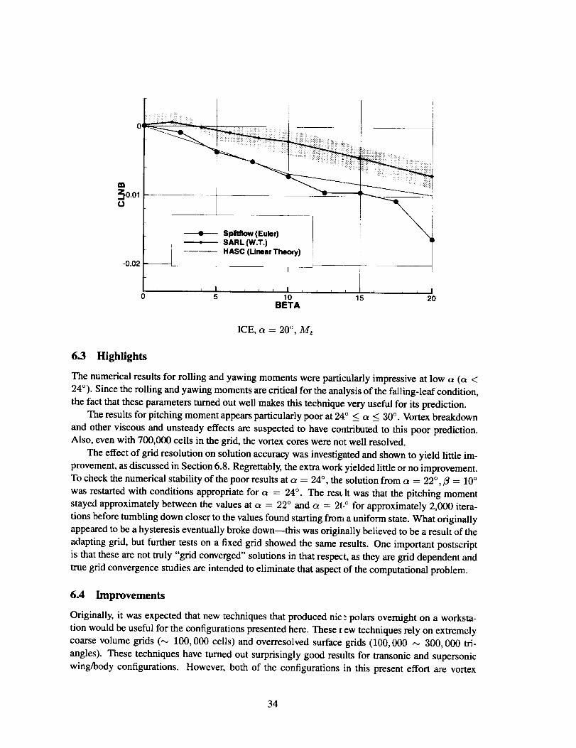
ICE, a = 20 °, Mz
6.3 Highlights
The numerical results for rolling and yawing moments were particularly impressive at low a (a <
24 °). Since the rolling and yawing moments are critical for the analysis of the falling-leaf condition,
the fact that these parameters turned out well makes this technique very useful for its prediction.
The results for pitching moment appears particularly poor at 24 ° < a < 30°. Vortex breakdown
and other viscous and unsteady effects are suspected to have contributed to this poor prediction.Also, even with 700,000 cells in the grid, the vortex cores were not well resolved.
The effect of grid resolution on solution accuracy was investigated and shown to yield little im-
provement, as discussed in Section 6.8. Regrettably, the extra work yielded little or no improvement.
To check the numerical stability of the poor results at a = 24°, the solution from a = 22 ° , B = 10°
was restarted with conditions appropriate for a = 24 °. The rest It was that the pitching moment
stayed approximately between the values at a = 22 ° and a = 2(, ° for approximately 2,000 itera-
tions before tumbling down closer to the values found starting from a uniform state. What originally
appeared to be a hysteresis eventually broke down--this was originally believed to be a result of the
adapting grid, but further tests on a fixed grid showed the same results. One important postscript
is that these are not truly "grid converged" solutions in that respect, as they are grid dependent and
true grid convergence studies are intended to eliminate that aspect of the computational problem.
6.4 Improvements
Originally, it was expected that new techniques that produced nic: polars overnight on a worksta-
tion would be useful for the configurations presented here. These few techniques rely on extremely
coarse volume grids (_ 100,000 cells) and overresolved surface grids (100,000 ,_ 300,000 tri-
angles). These techniques have turned out surprisingly good results for transonic and supersonic
wing/body configurations. However, both of the configurations in this present effort are vortex
34

dominated at the flow speeds and angles used here, and the vortices require a large number of cells
off the surface. Typically, convergence is delayed at the low speeds.
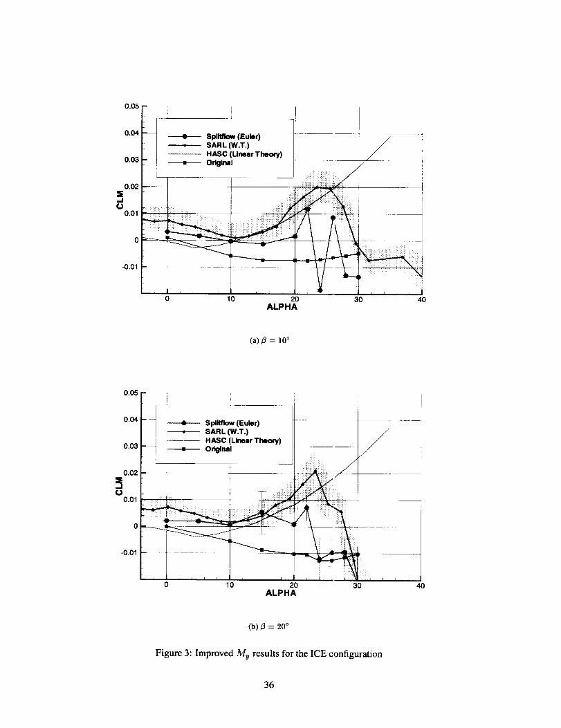
Figures 3(a) and 3(b) show a comparison of these results. "Original" refers to the first pass at
solution of these problems, which involves running SpliOqow on extremely coarse (approximately
100,000 cell) grids requiring only a few hours per case on a workstation. As shown in Figures 3(a)
and 3(b) the coarse grid techniques produced unusably poor data, while the techniques described
here did a reasonably good job of capturing the current nonlinear trends seen in the experimental
data.
Some of the nonlinearities displayed in the CFD results with increasing a may be due to the
complex vortical flows for these configurations. Disagreements have been found in results from
different wind tunnels for the ICE configuration. Results from a different wind tunnel test show
nonlinearities not apparent in the SARL tests.
35
0.05
0.04
0.03
0,02
(J0.01
-0.01
--_ ----e---- Splitllow (Euler)
SARL (W.T.)HASC (Unear Theory)Original
10 20ALPHA
30 40
(a) 13 = 10 °
Splltflow(Eu_dSARL(W.T.)HASC(UnearTheory)Original
0 10 20 30ALPHA
(b) _ = 20°
Figure 3: Improved Mu results for the ICE configuration
36
u -005
1
III
Sideslip Effects on Pitching Moment
--o-- Beta=0
---.m- Beta--10 __
Beta=10
Beta-20
---+-- Bet3=30 i
AOA (dell)
\,.
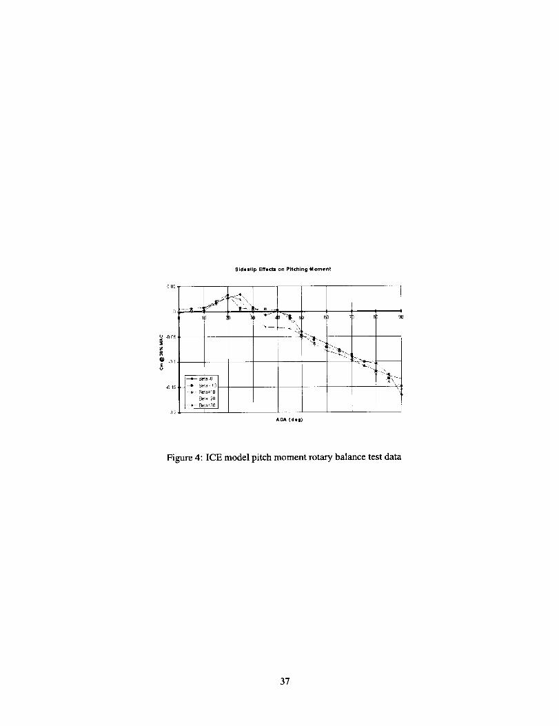
Figure 4: ICE model pitch moment rotary balance test data
37

Figure4 showspitchmomentcoefficient(My)testdatafortht:ICEmodelfromarotarybalancetestin 1996attheBhirleAppliedResearch10-footverticalwind.unnel in Neuberg, Germany [18].
The test used a 1/13th scale model with dynamic and static data cc_llection. Comparing Figures 3(b)
and 4 for/3 = 20 °, two important issues are the location of the curve crossing the axis and both
the Bhirle measurements and the SpliO'low computational results show a "leveling off" near 24°
around zero My, before the value drops negative. These differences lead to a conclusion that thereis some fundamental difference between the SARL wind tunnel tests and the inviscid simulations.
Since the Bhirle data is taken at "low" Reynolds number, and the SARL data is at "high" Reynolds
number, and inviscid simulations with Split]tow imply "low-but-not-controlled" viscosity (hence
"high" Reynolds number), it is expected that some Reynolds number effect is appearing in this
comparison.
6.5 Solution Adaption
Solution-based grid adaption was relied upon in Splitflow to yield highly-resolved solutions with
a minimum number of cells and without expert setup. SpliO'low can refine on many functions, but
how does one decide what is important? Traditionally at LMTAS, helicity (_- _) is used to adapt
the grid to vortices. However, the present results indicate that helicity does not resolve vortex cores
as well as expected, instead it tings the outside, as shown in Figure 5(a).
For configurations such as these that are highly dependent on proper vortex resolution, that is
not acceptable, so vorticity (H) was added as an adaption function to Omnigrid Spli_ow. Vorticity
does a much better job of locating the vortex cores, as shown in Figure 5(b) for the same conditions.
Note that with no solution adaption, as shown in Figure 5(c), the vortices do not even appear to have
been fully formed.
Even at the higher values of _ and/_, both of these configurations' flow solutions are vortex-
dominated. For flows that arc transonic or supersonic, vorticity and helicity would not locate the
shocks (and often yield a poor or unusable result). In those cases, either gradients of Mach number,
gradients of pressure, or divergence of density would most likely bt_used to refine on compressibility
effects. Resolving the flow features is very important, as failure t¢. do so may lead to very differentflow solutions.
For flows involving both shocks and shears, some balancing is required; however, most criteria
will setup a particular pattern of prioritization, without some sort of weighting that will probably
vary from one configuration to another [19]. In some sense, an acrodynamicist is required to have
an understanding of the approximate final solution before the computation can be completed. Cur-
rently, deciding on the set of adaption functions for a given flow is still much more an art than ascience.
6.6 Leading Edge Resolution
Traditionally for CFD analysis of lifting surfaces, sufficient leading edge resolution is important.
Leading edge resolution is more important for shock-driven flows, or flows where a shock location
sets the important results (particularly pitching moment, Mu). Th_se runs are not shock-driven, in
particular, but rather vortex driven, and this appears to make LE :°esolution less significant due to
the sharp leading edges. The leading edge resolution is shown in Figure 6 for an ICE configuration
at c_ = 24 ° and/3 = 10 °.
This leading edge resolution appears very coarse. Preferably, _he grid around the leading edge
would be dense enough for the individual grid lines to be indistinguishable at a full-size view for the
aircraft. When using Spli(flow or any comparable unstructured cooke, a certain amount of "smooth-
38

(a) Solution adaption with helicity, a = 24°, B = 10°
(b) Solution adaption with vorticity, a = 24 °,/3 = 10 °
(c) No solution adaption, a = 24°,/3 = 10°
Figure 5: Effect of different solution adaption parameters on computed vortex structure
39

Figure 6: Leading edge resolution for the ICE model
ing" is required to blend the fine-cells near the surface and the larger cells away from the aircraft.
In this case, if the cells were that tiny, nearly all of the available cell resources for grid adaption
would have been pulled to the leading and trailing edges of the wing leaving nothing left to resolve
the vortices without requiting unusably large grid sizes.
6.7 Convergence
Convergence is both a traditional measure and traditional difficulty for the successful use of CFD.
Because of the wide range of flow conditions, convergence on some cases was not expected. Further,
at higher a (and/3?), the expected flow should be unsteady and include significant viscous effects
(separation, reattachment, etc.)--under these conditions, a converged Euler solution is probably not
expected, and cautious interpretation is required.
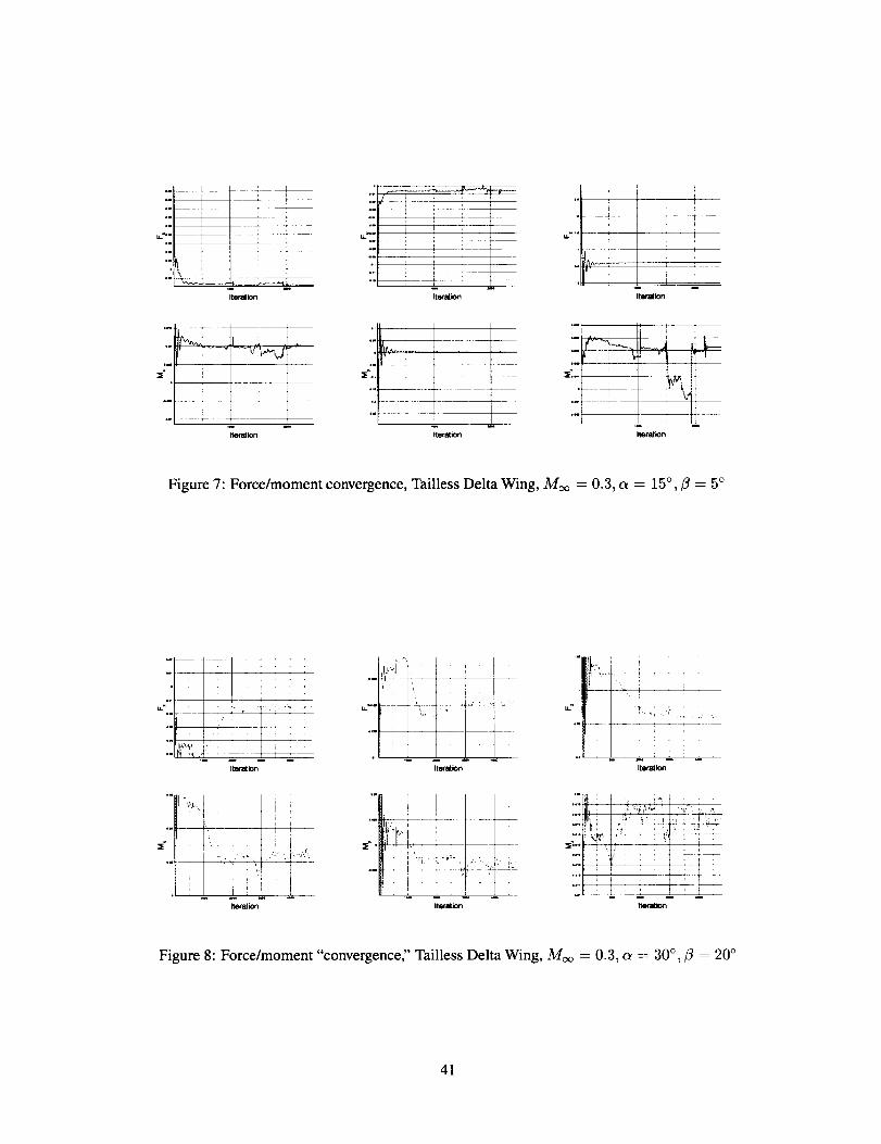
For some of these runs, the force and moment coefficients converged well, but convergence was
very sensitive to grid adaption. Figure 7 shows the convergence for each of the force and moment
coefficients for the typical case a = 15 ° and/3 = 5 ° . In these cases, some of the values converged
well, and others did not. Note also that the same values were reached at moderate and larger grid
sizes (greater than 300,000 cells).
Conversely, some of these runs featured very poor convergence properties. Figure 8 shows the
force and moment convergence for a = 30 ° and fl = 20°. Examining these plots, it is not clear that
anything is converging, much less what it might be converging towards.
6.8 Grid Convergence
Grid convergence studies were also performed on certain runs in an effort to determine why certain
runs turned out so poorly and if a finer grid would alleviate the problem. While it is unfortunate
40
.. i _ : -- " i
o. .. [ __.
" i
,-- m ,.
Iteralk_a Iteralion Iteralion
Iteration Iteration Iteralk:)n
Figure 7: Force/moment convergence, Tailless Delta Wing, M_ -- 0.3, a -- 15 °, fl = 5°
u."
i : !
...... i̧ -_; 1¸.̧......,/
Itermion Rer_ion
..1+/ !
:`Iteration
"L _1_ _ _ i _ °"
Itetalton Iteration
Figure 8: Force/moment "convergence" Tailless Delta Wing, A//_ = 0.3, cr = 30 ° , fl -- 20 °
41
400,000cells 800,000cells
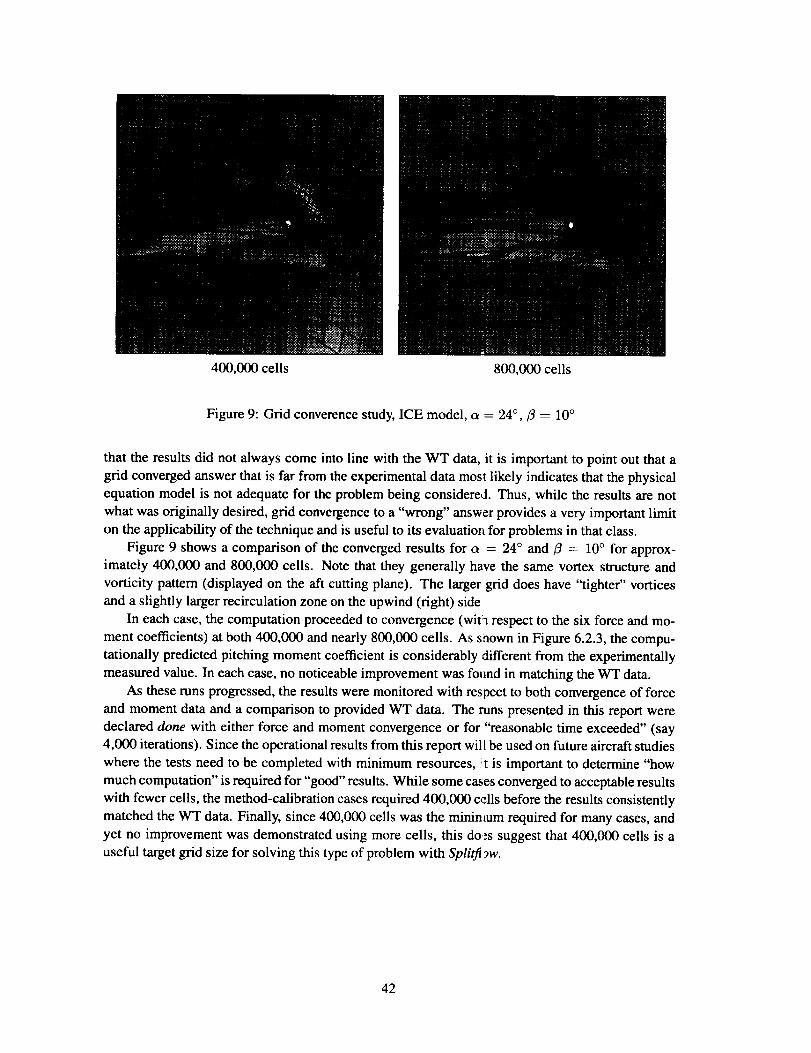
Figure9: Gridconverencestudy,ICEmodel,a = 24 °, fl ----10°
that the results did not always come into line with the WT data, it is important to point out that a
grid converged answer that is far from the experimental data most likely indicates that the physical
equation model is not adequate for the problem being considered. Thus, while the results are not
what was originally desired, grid convergence to a "wrong" answer provides a very important limit
on the applicability of the technique and is useful to its evaluation for problems in that class.
Figure 9 shows a comparison of the converged results for c_ = 24 ° and fl = 10° for approx-
imately 400,000 and 800,000 cells. Note that they generally have the same vortex structure and
vorticity pattern (displayed on the aft cutting plane). The larger grid does have "tighter" vortices
and a slightly larger recirculation zone on the upwind (right) side
In each case, the computation proceeded to convergence (wita respect to the six force and mo-
ment coefficients) at both 400,000 and nearly 800,000 cells. As stlown in Figure 6.2.3, the compu-
tationally predicted pitching moment coefficient is considerably different from the experimentally
measured value. In each case, no noticeable improvement was found in matching the WT data.
As these runs progressed, the results were monitored with respect to both convergence of force
and moment data and a comparison to provided WT data. The runs presented in this report were
declared done with either force and moment convergence or for "reasonable time exceeded" (say4,000 iterations). Since the operational results from this report will be used on future aircraft studies
where the tests need to be completed with minimum resources, it is important to determine "how
much computation" is required for "good" results. While some cases converged to acceptable results
with fewer cells, the method-calibration cases required 400,000 cells before the results consistently
matched the WT data. Finally, since 400,000 cells was the minimum required for many cases, and
yet no improvement was demonstrated using more cells, this do,_.s suggest that 400,000 cells is a
useful target grid size for solving this type of problem with SpliO_ _w.
42

-1513 129 -108 -0 87 -C 66 _0 45 4; 24 -0 03 018 039
Figure 10: Contour plot of Cp difference, ICE model at _ = 24° , fl = 10°
Regrettably, this test is only an approximation to true grid convergence. A complete grid con-
vergence test would involve using a sequence of different grids, in particular ones with consistent
refinements, to show that the solution obtained is independent of the grid. A final check on this
= 24°, 13 --= 10° case involved restarting the similar cases with conditions appropriate for theformer:
1. Restarting with the checkpoint solution for o_ = 22 °, fl = 10 °, and solving with grid adaption
until the forces and moments converged.
2. Restarting with the checkpoint solution for _ = 26 °, fl -- 10°, and solving with grid adaption
until the forces and moments converged.
3. Restarting with the checkpoint solution for o_ = 22°,/3 = 10°, and solving without grid
adaption until the forces and moments converged.
In all three cases, for over 1,000 iterations (and 50 grid adaption cycles where adaption was
used!), the computed forces and moments stayed between the values computed for the o_= 22 ° and
= 26° cases, before dropping to a value much closer to that predicted from a dead-start (and far
off the wind-tunnel data). While one would like to conclude that some aspect of the grid adaption
process is pulling the flow solution away from nature's solution towards a very different one, the
fact that the same solution was reached without adapting to the different flow suggests that this "way
off" value might be an appropriate solution to the inviscid flow field at these conditions. A contour
plot of ACp = Cpre,t_ - Cpd_.aast_,t is shown in Figure 10; one can see the lower pressure on theforward windward "strake" area and the strong higher pressure on the aft-most leeward area--the
difference in pitching moment is clear, but this intermediate position is simply not stable.
6.9 CPU Requirements
The inviscid computations presented in this report seemed to take considerably more CPU time than
expected. While these numbers are suspicious and being reviewed, a developmental version of Om-
43
O_
2
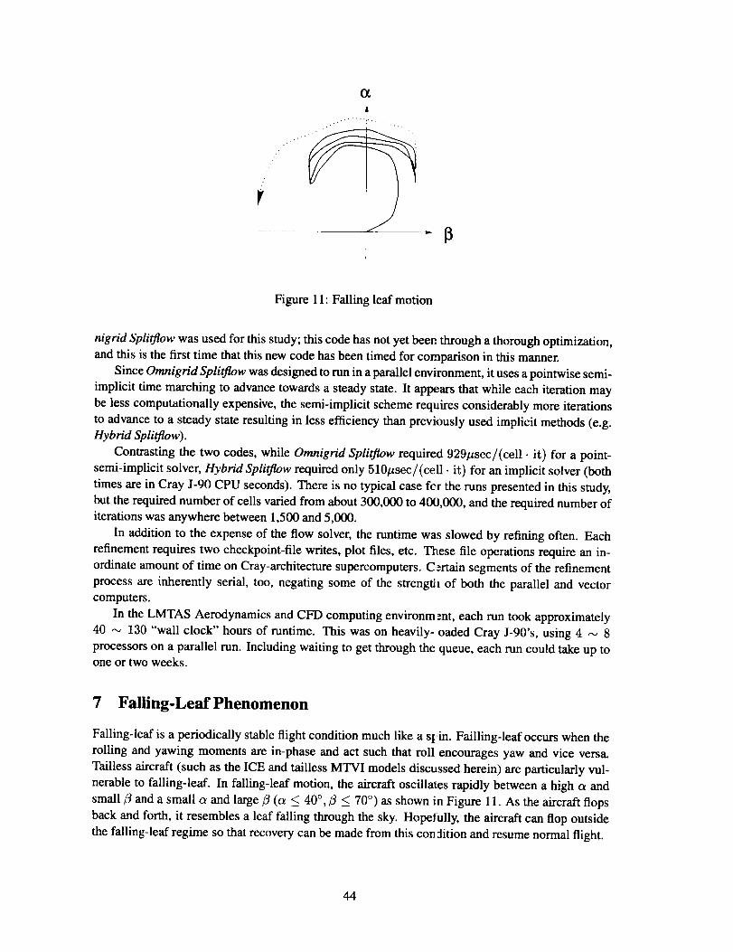
Figure 11: Falling leaf motion
nigrid SpliOqow was used for this study; this code has not yet been through a thorough optimization,
and this is the first time that this new code has been timed for comparison in this manner.
Since Omnigrid SpliO_ow was designed to run in a parallel environment, it uses a pointwise semi-
implicit time marching to advance towards a steady state. It appears that while each iteration may
be less computationally expensive, the semi-implicit scheme requires considerably more iterations
to advance to a steady state resulting in less efficiency than previously used implicit methods (e.g.Hybrid Splitflow).
Contrasting the two codes, while Omnigrid SpliO°_ow required 929#sec/(cell. it) for a point-
semi-implicit solver, Hybrid SpliO'_ow required only 510/zsec/(cell. it) for an implicit solver (both
times are in Cray J-90 CPU seconds). There is no typical case for the runs presented in this study,
but the required number of cells varied from about 300,000 to 400,000, and the required number ofiterations was anywhere between 1,500 and 5,000.
In addition to the expense of the flow solver, the runtime was slowed by refining often. Each
refinement requires two checkpoint-file writes, plot files, etc. These file operations require an in-
ordinate amount of time on Cray-architecture supercomputers. Certain segments of the refinement
process are inherently serial, too, negating some of the strength of both the parallel and vectorcomputers.
In the LMTAS Aerodynamics and CFD computing environment, each run took approximately
40 _ 130 "wall clock" hours of runtime. This was on heavily- oaded Cray J-90's, using 4 _ 8
processors on a parallel run. Including waiting to get through the queue, each run could take up toone or two weeks.
7 Falling-Leaf Phenomenon
Falling-leaf is a periodically stable flight condition much like a st:in. Failling-leaf occurs when the
rolling and yawing moments are in-phase and act such that roll encourages yaw and vice versa.
Tailless aircraft (such as the ICE and tailless MTVI models discussed herein) are particularly vul-
nerable to falling-leaf. In falling-leaf motion, the aircraft oscillates rapidly between a high o_and
small/3 and a small c_ and large/3 (a _< 40 °,/3 < 70 °) as shown in Figure 11. As the aircraft flops
back and forth, it resembles a leaf falling through the sky. Hopefully, the aircraft can flop outside
the falling-leaf regime so that recovery can be made from this condition and resume normal flight.
44

SRYP Nose-Slice
Departure
:,-iDepar,ture.._,
.,;, ;:]. ,,_,_ .: .
Cn
Stable
Dutch Roll
13DYN
i..._v
Figure 12: Falling leaf susceptibility region
Falling leaf analysis starts as in [20] with the definition of the Synchronous Roll-Yaw Parameter
(SRYP):Cn 3
SRYP ct3 += (1)l_,r,z Cn_
_-_-+ S__ -d-_l_Ixz
and the Dutch-roll stability parameter:
IZZ
Cn,3DVr_= Crib cos a -/_ Gn sin a
where the lateral stability derivative is:
oct0/7
and the directional stability derivative is:
OCn ACn
cn,- 0/7 A/7
given the moments of inertia for the ICE model (sl. ft2):
I_z = 35,479
Izz = 110,627
Ixz = -525
The falling leaf susceptibility region is defined by:
C_D_N > 0 N
asshown inFigure12.
AC_~C_A/7 /7
C_/7
SRYP > 0
(2)
(3)
(4)
(5)
(6)
(7)
(8)
45
ol
o7
o_e
o,s
o.s
o.2
o,t /I
-o,_
o
i ( 0.004
F'
SRYP - -'--1
_ 0.001
! " z
ALPHA
-0,002
-000_
(a) SARL test data
ALPHA
(b) Splitflow prediction
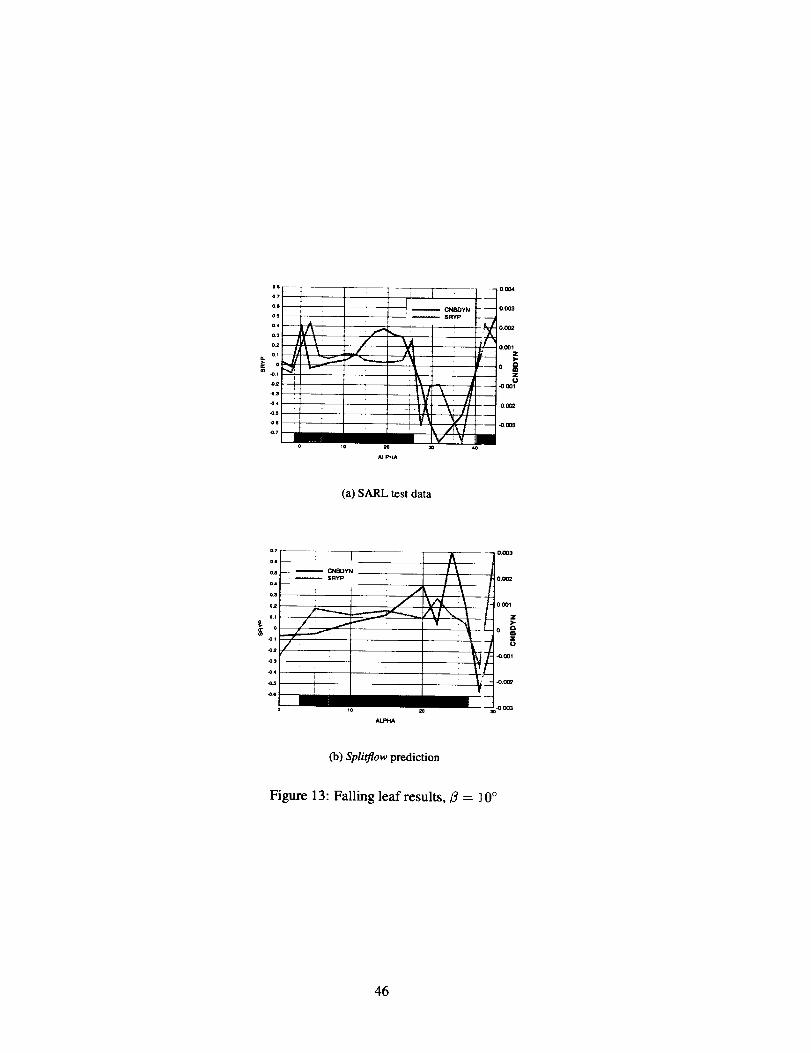
Figure 13: Falling leaf results, fl = ]0 °
46

w
os
os
o4
o3
0.2
ol
4_3
_ _ m 7 _
--- _ CNBDYN _1,_-. I
/
__ _ _ SRYP _ _ . _ ,
..... fl _\ /
' i
I
ALPHA
0003
00025
0.002
00015
0.001
O.O0(Z
o =0
-0.0015
-O.0_
_.0025
(a) SARL test data
oa
02
01
i - CNBDVNiSRYP i
y_ i
0002
0OO175
0 [X)15
0.00125
0001
0OO075
00005
o g
41.0_5
4%_75
-0.001
4_ 00125
_ -0.0015-O1:K)175
_o _°°Q
(b ) SpliOqow prediction
Figure 14: Falling leaf results,/3 = 20 °
47
O_
0.015
001
zO 0(;6
|o¢db._i
-O.Ol
-o.o15
I
CNBIDYN
BRYP
IIII /lll'l ' IT
/ 0,2
/0.1
(a) NASA Langley Research Center test data
0.5
\ _ °_0.0_ 0.2
01
I o
1t/ !
,L/\o,-O01 _ -O.4
m m
I i -o.s10 20 30 40
.IU.PHA
-O.oo6
(b ) Spli_ow prediction
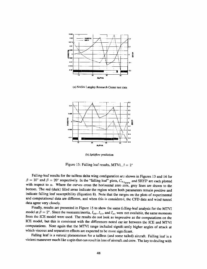
Figure 15: Falling leaf results, MTVI, ,7 = 2°
Falling-leaf results for the tailless delta wing configuration ar_- shown in Figures 13 and 14 for
¢3 = 10 ° and/3 = 20 ° respectively. In the "falling leaf" plots, Cr,3DVN and SRYP are each plotted
with respect to a. Where the curves cross the horizontal zero axis, grey lines are drawn to the
bottom. The red (dark) filled areas indicate the region where both parameters remain positive and
indicate falling leaf susceptibility (Equation 8). Note that the rar.ges on the plots of experimental
and computational data axe different, and when this is considere, l, the CFD data and wind tunnel
data agree very closely.
Finally, results are presented in Figure 15 to show the same t_tiling-leaf analysis for the MTVI
model at/3 = 2 °. Since the moments inertia, Ix_, Izz, and I_z were not available, the same moments
from the ICE model were used. The results do not look as impressive as the computations on the
ICE model, but this is consistent with the differences noted earlier between the ICE and MTVI
computations. Note again that the MTVI range included signifi-antly higher angles of attack at
which viscous and separation effects are expected to be more significant.
Falling leaf is a natural phenomenon for a tailless (and some tailed) aircraft. Falling leaf is a
violent maneuver much like a spin that can result in loss of aircraft and crew. The key to dealing with
48
falling leaf is being both able to avoid it and to recover from an inadvertant entry. One importantconclusion from this data is that control augmentation will be required at all a for this class of
aircraft--in particular, the use of an active control system will probably be needed to avoid a falling
leaf condition. While this report is oriented towards tactical aircraft, other classes of aircraft shaped
similarly may also suffer from a tendency towards falling leaf, making this analysis important for
non-military aircraft as well (e.g. a flying-wing transport configuration).
8 Conclusions
Much of the desired data can be accurately computed, but often these large nonlinear problems re-
quire large grids and longer runtimes than anticipated. At LMTAS, the S&C group desires complete
polar analysis in hours, which is not practical with most Euler methods, and Preliminary Design
wants a solution per hour, which is definitely not practical today. Also, there were no black boxes
here, with each run requiring professional aerodynamic assistance to nurture it to a proper comple-
tion.
The problem of how to do rapid aerodynamic predictions for high-performance aircraft design
requires more investigation. Several issues are clear:
1. Linear methods do not provide useful data through nonlinear flow regimes.
2. Inviscid methods do not provide useful data through viscous flow regimes.
3. Methods that are fast for one class of problem (e.g. transonic wing/fuselages) may get bogged
down on different problems (e.g. high-a delta/wings).
4. It is difficult to incorporate massive computing into the rapid cycle of aircraft design--unless
the required data cannot be reasonably obtained otherwise or guessed at.
These problems seem to imply that a fast method is needed for the automatic solution of aero-
dynamic problems using the Navier-Stokes equations to capture both compressible and viscous
effects. Clearly, automatic grid generation and adaptation is still important, as without appropriate
grids, the process is doomed. CL, CM, and CDo are critical values, although they can be computed
with proper techniques and sufficient patience with the correct physical models. But research needs
to proceed in the development of CFD grid generators and flow solvers.The motivation for this effort is to advance the routine use of CFD in the design of high-
performance aircraft by obtaining sufficient accuracy, reducing the time required, and producing
codes that are easy to use. While the times required for the simulations presented here are larger
than desirable, and effort is still required regarding interface and usability, goal of routine usage
of CFD in design is progressing well. Advanced design was already using CFD routinely; along
with some of these results regarding using SpliOqow at high angles of attack and slip, S&C is now
starting to use these same methods for concept aircraft derived from the ICE model. Finally, these
techniques may be used soon outside of LMTAS to solve related problems in high-performance
aircraft design.
8.1 Future Efforts
The Aerodynamics & CFD group at LMTAS is working to develop a completely new version of
the Spli([low automatic grid generator and flow solver in an effort to easily generate good solutions
for either inviscid or viscous analysis. Since numerous difficulties have arisen due to the strangely
49
shapedcellsonthesurfaceof theoctreegrid,thecurrenteffortfo.'usesonr: cing the cell cutting
logic with cell projection. The goal is to automatically produce I ree-like m. _ s that have smooth
near-surface grids suitable for modeling of viscous shear layers. "'his methot_ _presents an attempt
to automate the production of a mesh suitable for viscous flow analysis.
Figure 16 shows some of the most recent results from this new code for the ICE model described
in this report. The smoother surface mesh is clearly visible, as is the resultant smooth surface
pressure contours. While adaptation is currently being implemented in the new code, it should
function the same way as the current versions of SpliO'tow.
An advantage of this new method is that the user can now allow adaptation within the viscous
shear layers all the way to the surface. A possible disadvantage is that either adaption criteria must
be useful in both the off-surface inviscid regions and the near-,'_urface viscous regions, or some
method must be created to separate the two.
These grids are also much smoother with respect to neighboring volume ratios, which could of-
ten be nearly unbounded with traditional octree methods 0; "_ 101°) • Meaningless grid parameters
such as body tolerance have been replaced with physical parameters like gap size, and the sliver
cells that produce cells many orders of magnitude smaller than their neighbors can be eliminated
altogether.
50

I I I i I I I I I
i(a) Oblique view (b) New surface mesh
(c) Pressure contours (top) (d) Pressure contours (bottom)
Figure 16: New grid generation method
51

9 Acknowledgments
Any large project such as this has many contributors. In particular, the author would like to thank
Professor David Darmofal and Dr. Andrew Cary for help in understanding vortex breakdown, Paul
McClure from our Advanced Design group, Ken Dorsett from S&C, and Keith Jordan for the sur-
face preparation of both the MTVI and ICE models. Splitflow support was provided by Dr. Neal
Domel, Dr. Steve Karman, Tracy Welterlen, and Dr. Brian Smith. Finally, both Jim Robarge, the
LMTAS program manager, and Farhad Ghalfari, the NASA program manager, were very helpful
with oversight and suggestions throughout the program.
52

References
[1]
[21
[3]
D. B. Finley, "Euler technology assessment program for preliminary aircraft design employing
splitflow code with cartesian unstructured grid method" NASA CR-4649, March 1995.
T. A. Kinard, B. W. Harris, and P. Raj, "An assessment of viscous effects in computational
simulation of benign and burst vortex flows on generic fighter wind-tunnel models using team
code," NASA CR-4650, March 1995.
D. A. Treiber and D. A. Muilenberg, "Euler technology assessment for preliminary aircraft
design employing overflow code with multiblock structured-grid method" NASA CR-4651,
March 1995.
[4] D. B. Finley and S. L. Karman, Jr., "Euler technology assessment for preliminary aircraft
design - compressibility predictions by employing the cartesian unstructured grid splitflow
code," NASA CR-4710, 1996.
[51 T. A. Kinard and P. Raj, "Euler technology assessment for preliminary aircraft design - com-
pressibility predictions by employing the unstructured grid usm3d code" NASA CR-4711,March 1996.
[6]
[7]
T. A. Kinard, D. B. Finley, and S. L. Karman, Jr., "Prediction of compressibility effects using
unstructured euler analysis on vortex dominated flow fields" AIAA 96-2499, June 1996.
J. K. Jordan, "Euler technology assessment--splitflow code applications for stability and con-
trol analysis on an advanced fighter model employing innovative control concepts" NASA
CR-1998-206943, March 1998.
[8] T. R. Michal, "Euler technology assessment for preliminary aircraft design -- unstruc-
tured/structured grid NASTD application for aerodynamic analysis of an advanced fighter/tail-
less configuration," NASA CR-1998-206947, March 1998.
[9] F. Ghaffari, "personal communication" January 1998. NASA Langley Research Center.
[10] A. Beguelin, J. J. Dongarra, G. A. Geist, W. Jiang, R. Manchek, K. Moore, and V. S. Sunderam,
"'PVM 3 user's guide and reference manual" ORNL TM-12187, May 1993.
[11] B.R. Smith, "The k-kl turbulence model and wall layer model for compressible flows," AIAA
90-1483, 1990.
[12] B. R. Smith, "A near wall model for the k-l two equation turbulence model" AIAA 94-2386,
1994.
[13] B. R. Smith, "personal communication re: k-kl turbulence model" unpublished, July 1998.
[14] M. J. Logan, ed., Proceedings of the Non-Linear Aero Prediction Requirements Workshop,March 1994. NASA CP-10138.
[15] S.L. Kannan, Jr., SPLITFLOW User's Manual: Preliminary Copy; Very Rough Draft. Lock-
heed Martin Tactical Aircraft Systems, Fort Worth, TX, February 1997.
[16] Amtec Engineering, Inc., P.O. Box 3633, Bellevue, WA 98009-3633, Tecplot, Interactive Data
Visualization for Scientists and Engineers, 6 ed., 1994.
53

[17] A. E.Albright,"Modificationandvalidationof conceptual design aerodynamic predictionmethod HASC95 with VTXCHN" NASA CR-4712, March 1996.
[18] K. M. Dorsett, S. E Fears, and H. E Houlden, "Innovative control effectors (ICE) phase II,"
Wright Laboratory WL-TR-97-3059, August 1997.
[19] E.F. Charlton, An Octree Solution to Conservation-laws overArbitrary Regions (OSCAR) with
Applications to Aircraft Aerodynamics. PhD thesis, The University of Michigan, 1997.
[20] J.V. Foster, "Analysis of"falling leaf" motion of class IV airplanes, status update" slides from
a talk, July 1995. Flight Dynamics Working Group Meeting, NAWC, Patuxent River, MD.
54


REPORT DOCUMENTATION PAGE Fo_,_,_,,_OMB No. 0704-0188
Public reporting burden for this c_lection of information is estimated to average 1 hour per response, ircJuding the time for reviewing instructions, searching exiting dalesoumm_, gathering and m_ntaining the deta needed, end compte_ng and reviewing the coMection of in_ormetion. Send comments i'ogerdtng this burden estimate or any ol_eraspect of this coJlection of information, including suggestions for reducing this burden, to Washington Psedquartem Sen_ces, Directorate for Information Operations andReports, 1215 Jofforaon Davis Highway, Suite 1204, Arlington, VA 2221_-4302, and to the Office of I_ anegement and Budget, Paperwork Reduction Project (0704-0188),Washingfo_ DC 20503.
1. AGENCY USE ONLY (Leave blank) 2. REPORT DATE 3. REPORT TYPE AND DATES COVERED
September 1998 Contractor Report
4. TITLE AND SUBTITLE 5. FUNDING NUMBERS
Numerical Stability and Control Analysis Towards Falling Leaf PredictionCapabilities of Splitflow for Two Genetic High-Performance Aircraft NAS 1-96014, Task 15Models WU 522-22-31-01
S.AUTHOR(S)Eric F. Charlton
7. PERFORMINGORGANIZATIONNAME(S)ANDADDRESS(ES)Lockheed-Martin Tactical Aircraft SystemsFort -Worth, TX 76101
9. SPONSORING/MONITORING AGENCY NAME(S) AND ADDRESS(ES)
National Aeronautics and Space AdministrationLangley Research CenterHampton, VA 23681-2199
8. PERFORMING ORGANIZATION
REPORT NUMBER
10. SPONSORING/MONITORING
AGENCY REPORT NUMBER
NASA/CR- 1998-208730
11. SUPPLEMENTARY NOTES
This study was performed by Lockheed-Martin Tactical Aircraft Systems under subcontract to Lockheed-MartinEngineering & Sciences, Hampton Virginia under contract to NASA Langley Research Center.Langley Technical Monitor: Mr. Farhad Ghaffari
12a.DISTRIBUTION/AVAILABILITYSTATEMENT
Unclassified-Unlimited
Subject Category 2 Distribution: StandardAvailability: NASA CASI (301) 621-0390
12b. DISTRIBUTION CODE
13. ABSTRACT (Maximum 200 words)
Aerodynamic analysis are performed using the Lockheed-Martin Tactical Aircraft Systems (LMTAS) Splitflowcomputational fluid dynamics code to investigate the computational prediction capabilities for vortex-dominatedflow fields of two different tailless aircraft models at large angles of attack and sideslip. These computations areperformed with the goal of providing useful stability and control data to designers of high performance aircraft.Appropriate metrics for accuracy, time, and ease of use are deterrrtined in consultations with both the LMTASAdvanced Design and Stability and Control groups. Results are obtained and compared to wind-tunnel data for
all six components of forces and moments. Moment data is combined to form a "falling leaf" stability analysis.Finally, a handful of viscous simulations were also performed to further investigate nonlinearities and possibleviscous effects in the differences between the accumulated inviscid computational and experimental data.
14. SUBJECT TERMS
Computational Fluid Dynamics, Euler/Navier-Stokes, Preliminary.' Aircraft Design,
Falling-Leaf Phenomenon, Vortical Flows, Cartesian/Unstructure ]-Grid Splitflow
17. SECURITY CLASSIFICATION
OF REPORT
Unclassified
18. SECURITY CLASSIFICATION
OF THIB PAGE
Unclassified
19. SECURITY CLASSIFICATION
OF ABSTRACT
Unclassified
15. NUMBER OF PAGES
5916. PRICE CODE
A04
20. LIMITATION
OF ABSTRACT
NBN 7540-01-280-5500 Standard Form 298 (Rev. 2-8_Prescribed by ANSI Std. Z-39-18298-102