numerical study of hydraulic jumps on corrugated beds...

Turkish J. Eng. Env. Sci.33 (2009) , 61 – 72.c© TUBITAKdoi:10.3906/muh-0901-7

Numerical study of hydraulic jumps on corrugated beds usingturbulence models

A. ABBASPOUR, D. FARSADIZADEH,A. HOSSEINADEH DALIR and A. A. SADRADDINI

Water Engineering Department, University of Tabriz,5166616471, Tabriz-IRAN.e-mail: [email protected]

Received 12.01.2009

AbstractHydraulic jumps have been used for dissipation of kinetic energy downstream of hydraulic structures,

such as spillways, chutes, and gates. It was found that if jumps were made to occur on corrugated beds,

tail water and length of jumps reduced significantly. During the formation of the hydraulic jump on a

corrugated bed, the flow is turbulent water and air mixing together. In the present study, 2-dimensional

numerical simulation of hydraulic jump on a corrugated bed was evaluated using both standard k-ε and

RNG k-ε models. The free surface was determined using the VOF method. The results showed that k-ε

turbulent model and VOF method for predicting the water surface in the jump on a corrugated bed were

suitable and the relative error of predicted water surface profiles and measured value were within a range

of 1%-8.6%. The study of the axial velocity profiles at different sections in the jump found that velocity

profiles in different experiments were similar and there was a good agreement between modeled and measured

results. The effects of corrugations (t, s) on the basic characteristics of jump, such as free surface location,

velocity, and shear stress distribution, were studied for a different range of Froude number.

Key Words: Hydraulic jump, corrugated bed, Navier-Stokes equations, volume of fluid (VOF), k-ε turbu-

lence models.

Introduction

Hydraulic jump in a horizontal channel with a smooth bed has been studied extensively by many researchers(Vischer and Hager, 1995). Recently, some investigations have been carried out on rough and corrugated beds.However, the main concern with jumps on rough and corrugated beds is that the roughness elements and crestof corrugations might be subjected to cavitations and erosion thereby may damage the structure itself. Previousresearch conducted by Ead et al. (2000) showed that if the crests of corrugations are placed at the level ofupstream bed carrying the supercritical flow, the corrugations would not protrude into the flow, hence preventcavitations in the basin. Furthermore, they also reported that, in culvert with corrugated bed, Reynolds shearstresses are produced so the velocity field above the corrugations is reduced.

Ead and Rajaratnam (2002) studied hydraulic jumps on a corrugated bed experimentally in the range of

Froude numbers from 4 to 10. Three values of the relative roughness t/y1 (t is the height of corrugations and y1

61

ABBASPOUR, FARSADIZADEH, HOSSEINADEH DALIR, SADRADDINI

is the initial depth of flow) 0.50, 0.43, and 0.25 were studied. Tokyay (2005) investigated the effect of channelbed corrugations on a hydraulic jump experimentally. In the experiments 2 values of wave steepness, 0.20 and0.26, were used and the range of Froude numbers was from 5 to 12. The results showed that many factors, suchas initial depth of flow, supercritical Froude number, height and wave length of corrugations t, s were effectiveon the characteristics of the hydraulic jump.

Study of hydraulic jump on corrugated beds by analytical methods is tedious not only because of boundarylayer problems but also due to complexity of turbulent flow and diffusion process involved between walls, bed,and rolling water surface. Hydraulic jump is a 2-phase turbulent flow and simulation of it by using turbulencemodels and VOF (volume-of-fluid) method can led to accurate results.

Gharangik and Chaudhry (1991) investigated a hydraulic jump by a numerical model. They applied theBoussinesq equations to simulate both the sub and supercritical flows and a hydraulic jump in a rectangularchannel having a small bed slope. The numerical study of hydraulic jump on a smooth bed has also been carriedout by Zhao and Misra (2004). The governing equations are the continuity and momentum for incompressibleflow and based on the 2-dimensional k-ε turbulence model. They used the VOF and the scale turbulencemodel to predict water surface location and horizontal velocity. Sarker and Rhodes (2002) studied hydraulicjump on a smooth bed by physical and numerical methods. They used the RNG k-ε turbulence model incombination with the volume of fluid (VOF) method for free surface modeling. There was a good agreement

between the 2-dimensional CFD solution and the physical measurements. Gonzalez and Bombardelli (2005)

simulated a hydraulic jump on a smooth bed using k-ε turbulence and Large Eddy Simulation (LES) models.The simulated results were compared with observations of mean flow and turbulence in hydraulic jumps by Liuet al. (2004).

The objective of this research was to investigate the numerical model of hydraulic jump on a corrugated bedusing standard and RNG k-ε turbulence models. This study was carried out with a CFD program, which usesthe finite-volume method to solve 2D Reynolds-averaged Navier Stokes (RANS) equations. In this program,

the free surface location is computed using the VOF (volume-of-fluid) method.

Materials and Methods

Governing equations

The governing equations are unsteady incompressible 2-dimensional continuity and Reynolds-averaged Navier-Stokes equations for liquid and air (Liu et al., 2002).

∂ρ

∂t+

∂

∂xi(ρui) = 0 (1)

∂

∂t(ρuj) +

∂

∂xi(ρuiuj) = − ∂P

∂xj+

∂

∂xi(μ + μt)

(∂ui

∂xj+

∂uj

∂xi

)+ ρgj (2)

ρ = αAρA + αwρw (3)

μ = αAμA + αwμw (4)

where ui is the velocity components, αA and αw are the volume fraction of air and water, ρA, ρw, and ρ arethe density of air, water, and mixture respectively; P is the pressure; g is the acceleration due to gravity. The

62


parameters of μ, μA,μw, and μt are the viscosity of mixture, air, water, and the eddy viscosity, respectively.

The turbulent viscosity, μt, is computed by combining k and ε as follows:

μt = ρCμk2

ε(5)

where Cμ = 0.09 is a constant

Numerical model

In the present research, hydraulic jump on a corrugated bed was numerically studied for different Froudenumbers using the k-ε models and the 2-phase flow theory.

Volume of fluid (VOF ) The water surface location was determined with the volume of fluid (VOF) method.

The VOF method uses a function F(x, y, t) to assign the free surface. The function F is obtained from thefollowing equation

∂F

∂t+ uj

∂F

∂xj= 0 (6)

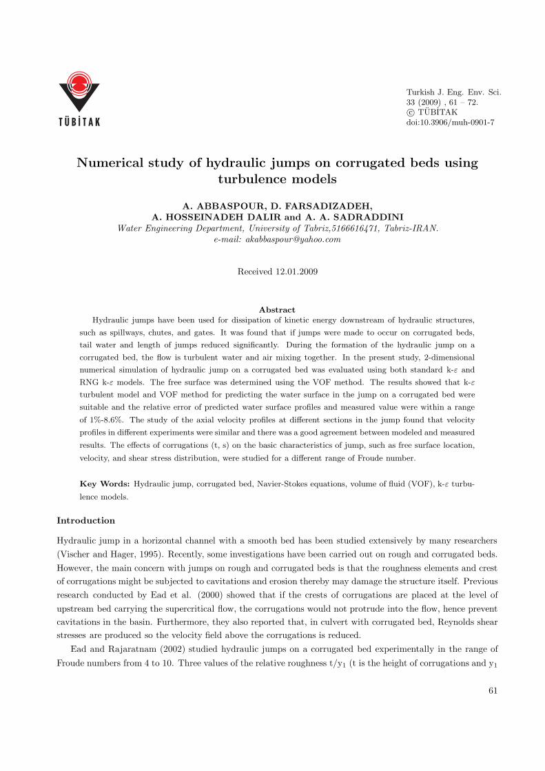
A unit value of F corresponds to a cell full of fluid, while a zero value indicates that the cell contains no fluid.Cells with F values between 0 and 1 contain a free surface. The function F can be solved with different methods.In this study a geometric reconstruction method was used. The geometric reconstruction scheme representsthe interface between fluids using a piecewise-linear approach. This scheme is the most accurate one and isapplicable for general unstructured meshes. In Figure 1 the interface between 2 fluids are represented for actualand the geometric reconstruction scheme.

Turbulence models In this study the hydraulic jump was modeled using 2-equation turbulence models in-cluding standard k-ε and RNG k-ε.

(a) (b)

Figure 1. Interface Calculations; (a) actual interface shape; (b) the geometric reconstruction scheme.

Standard k-ε model Standard k-ε model is given by the following equations:

ρui∂k

∂xi= μt

(∂uj

∂xi+

∂ui

∂xj

)∂uj

∂xi+

∂

∂xi

{(μt/σk)

∂k

∂xi

}− ρε (7)

63


ρui∂ε

∂xi= C1ε

( ε

k

)μt

(∂uj

∂xi+

∂ui

∂xj

)∂uj

∂xi+

∂

∂xi

{(μt/σε)

∂ε

∂xi

}− C2ερ

(ε2

k

)(8)

where k is turbulent kinetic energy and ε is dissipation rate. σk = 1 and σε = 1.3 are the turbulent Prandtlnumbers for k and ε, respectively. C1ε = 1.44 and C2ε = 1.92 are empirical constants.

RNG k-ε model The equations of RNG k-ε model are as following (Papageorgakis and Assanis, 1999):

ρui∂k

∂xi= μtS

2 +∂

∂xi

(αkμeff

∂k

∂xi

)− ρε (9)

ρui∂ε

∂xi= C1ε

( ε

k

)μtS

2 +∂

∂xi

(αεμeff

∂ε

∂xi

)− C2ερ

(ε2

k

)− R (10)

The term R is modeled as

R ≡Cμρη3(1 − η/η0

)

1 + βη3

ε2

k(11)

η ≡ Sk

ε(12)

S ≡√

2SijSij , Sij ≡ 12

(∂uj

∂xi+

∂ui

∂xj

)(13)

where αk = αε = 1.39, C1ε = 1.42, C2ε = 1.68, η0 = 4.38, and β = 0.012 are model constants. R and S areadditional terms related to the mean rate of strain and turbulence quantities.

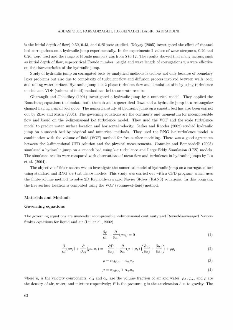
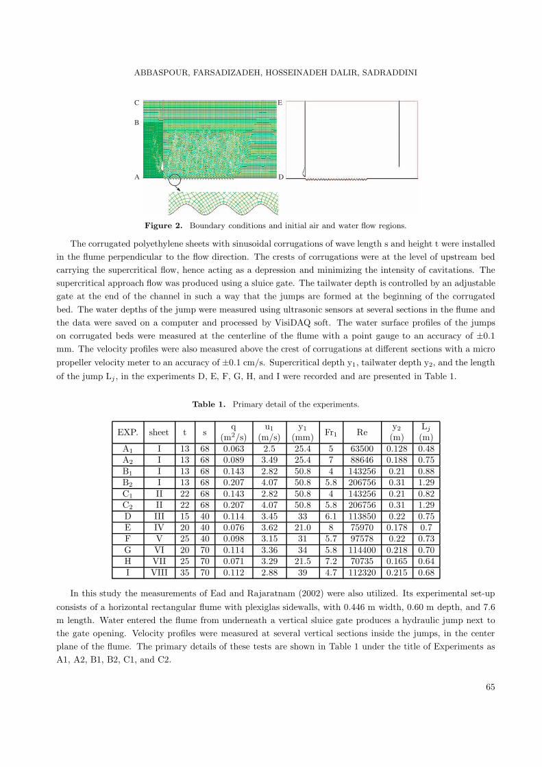
Model geometry and boundary conditions To analyze the hydraulic jump on a corrugated bed, the modelgeometry was generated and the unstructured grids were created. Considering small height of corrugations, thegrids size near the corrugated bed was in the range of 5-9 mm, and for the rest of computational region, it wasin the range of 10-22 mm. The view sketch of the initial regions and boundary conditions in the jump on thecorrugated bed are shown in Figure 2.

The basic procedure is to define primary phase water and a secondary phase air as shown in Figure 2. Asshown in Figure 2, the inlets were defined as the water flow (AB) and air flow (BC) into the domain. The

boundary conditions also were defined as wall boundary condition (channel bed and gates), streamwise velocity

or hydrostatic pressure inlets (AB), hydrostatic pressure inlet (BC), and outlet (DE) equal to zero. The values

of the velocity and the turbulence parameters, i.e., the turbulent kinetic energy (k) and the dissipation (ε), wereobtained from experimental data. To calculate the effect of the wall on the flow, empirical wall functions, knownas standard equilibrium, were used. The time-dependent solution procedure was given an initial condition inwhich all of the cells upstream of the gate and up to velocity inlets level were patched as water filled; F =1.

Experimental procedure

The experiments were conducted in a metal-glass flume of rectangular cross section. The flume has the dimen-sions of 0.25 m width, 0.5 m depth, and 10 m length with a slope of 0.002. The flume is equipped with a sluicegate at the entrance and discharge was measured by a triangular weir placed at the end of it.

64


C

A D

B

E

Figure 2. Boundary conditions and initial air and water flow regions.

The corrugated polyethylene sheets with sinusoidal corrugations of wave length s and height t were installedin the flume perpendicular to the flow direction. The crests of corrugations were at the level of upstream bedcarrying the supercritical flow, hence acting as a depression and minimizing the intensity of cavitations. Thesupercritical approach flow was produced using a sluice gate. The tailwater depth is controlled by an adjustablegate at the end of the channel in such a way that the jumps are formed at the beginning of the corrugatedbed. The water depths of the jump were measured using ultrasonic sensors at several sections in the flume andthe data were saved on a computer and processed by VisiDAQ soft. The water surface profiles of the jumpson corrugated beds were measured at the centerline of the flume with a point gauge to an accuracy of ±0.1mm. The velocity profiles were also measured above the crest of corrugations at different sections with a micropropeller velocity meter to an accuracy of ±0.1 cm/s. Supercritical depth y1, tailwater depth y2, and the lengthof the jump Lj , in the experiments D, E, F, G, H, and I were recorded and are presented in Table 1.

Table 1. Primary detail of the experiments.

EXP. sheet t sq u1 y1 Fr1 Re

y2 Lj

(m2/s) (m/s) (mm) (m) (m)A1 I 13 68 0.063 2.5 25.4 5 63500 0.128 0.48A2 I 13 68 0.089 3.49 25.4 7 88646 0.188 0.75B1 I 13 68 0.143 2.82 50.8 4 143256 0.21 0.88B2 I 13 68 0.207 4.07 50.8 5.8 206756 0.31 1.29C1 II 22 68 0.143 2.82 50.8 4 143256 0.21 0.82C2 II 22 68 0.207 4.07 50.8 5.8 206756 0.31 1.29D III 15 40 0.114 3.45 33 6.1 113850 0.22 0.75E IV 20 40 0.076 3.62 21.0 8 75970 0.178 0.7F V 25 40 0.098 3.15 31 5.7 97578 0.22 0.73G VI 20 70 0.114 3.36 34 5.8 114400 0.218 0.70H VII 25 70 0.071 3.29 21.5 7.2 70735 0.165 0.64I VIII 35 70 0.112 2.88 39 4.7 112320 0.215 0.68

In this study the measurements of Ead and Rajaratnam (2002) were also utilized. Its experimental set-upconsists of a horizontal rectangular flume with plexiglas sidewalls, with 0.446 m width, 0.60 m depth, and 7.6m length. Water entered the flume from underneath a vertical sluice gate produces a hydraulic jump next tothe gate opening. Velocity profiles were measured at several vertical sections inside the jumps, in the centerplane of the flume. The primary details of these tests are shown in Table 1 under the title of Experiments asA1, A2, B1, B2, C1, and C2.

65


Results and Discussion

Standard and RNG turbulent models were used to simulate the hydraulic jump on corrugated bed and thecharacteristics of jump, such as water surface profile, length of the jump, velocity profile in different sections,and bed shear stress were evaluated.

Water surface profile

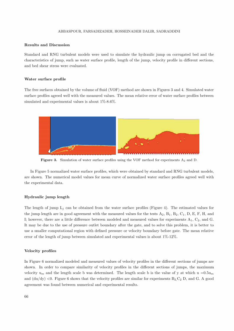
The free surfaces obtained by the volume of fluid (VOF) method are shown in Figures 3 and 4. Simulated watersurface profiles agreed well with the measured values. The mean relative error of water surface profiles betweensimulated and experimental values is about 1%-8.6%.

Figure 3. Simulation of water surface profiles using the VOF method for experiments A2 and D.

In Figure 5 normalized water surface profiles, which were obtained by standard and RNG turbulent models,are shown. The numerical model values for mean curve of normalized water surface profiles agreed well withthe experimental data.

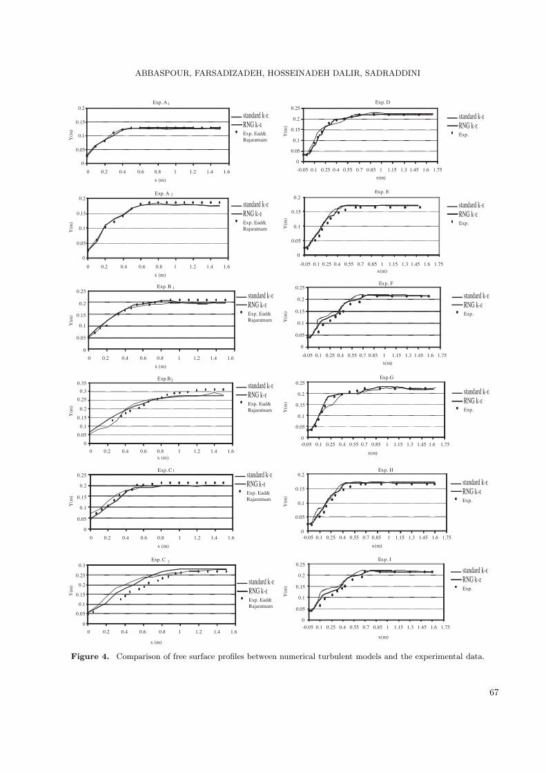
Hydraulic jump length

The length of jump Lj can be obtained from the water surface profiles (Figure 4). The estimated values for

the jump length are in good agreement with the measured values for the tests A2, B1, B2, C1, D, E, F, H, andI; however, there are a little difference between modeled and measured values for experiments A1, C2, and G.It may be due to the use of pressure outlet boundary after the gate, and to solve this problem, it is better touse a smaller computational region with defined pressure or velocity boundary before gate. The mean relativeerror of the length of jump between simulated and experimental values is about 1%-12%.

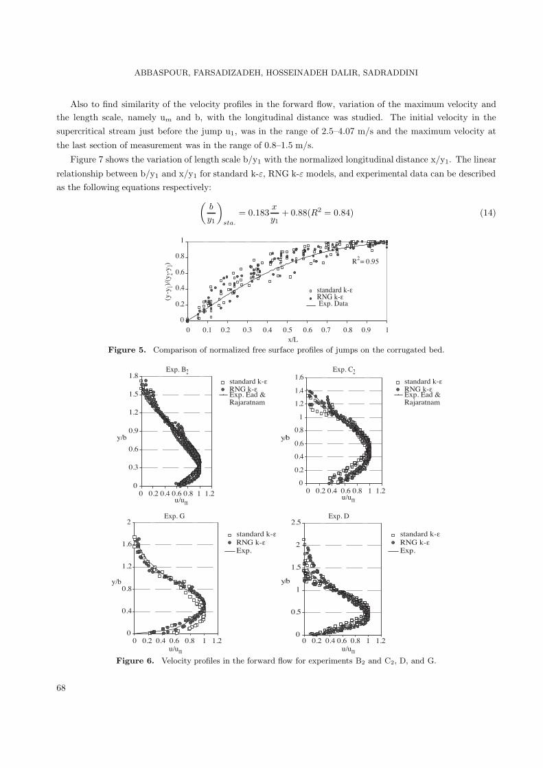
Velocity profiles

In Figure 6 normalized modeled and measured values of velocity profiles in the different sections of jumps areshown. In order to compare similarity of velocity profiles in the different sections of jumps, the maximumvelocity um and the length scale b was determined. The length scale b is the value of y at which u =0.5um

and (du/dy) <0. Figure 6 shows that the velocity profiles are similar for experiments B2,C2 D, and G. A good

agreement was found between numerical and experimental results.

66


Exp. A 1

0

0.05

0.1

0.15

0.2

Exp. A 2

0

0.05

0.1

0.15

0.2

Exp. D

0

0.05

0.1

0.15

0.2

0.25

-0.05 0.1 0.25 0.4 0.55 0.7 0.85 1 1.15 1.3 1.45 1.6 1.75

x(m)

Exp. E

0

0.05

0.1

0.15

0.2

-0.05 0.1 0.25 0.4 0.55 0.7 0.85 1 1.15 1.3 1.45 1.6 1.75x(m)

Exp. Ead&Rajaratnam

Exp. Ead&Rajaratnam

Exp.

Exp.

0 0.2 0.4 0.6 0.8 1 1.2 1.4 1.6

x (m)

0 0.2 0.4 0.6 0.8 1 1.2 1.4 1.6

x (m)

0.25

0.2

0.15

0.1

0.05

0

Exp. B 1

Exp.B2

0.25

0.3

0.35

0.2

0.15

0.1

0.05

0

Exp. F

0

0.05

0.1

0.15

0.2

0.25

-0.05 0.1 0.25 0.4 0.55 0.7 0.85 1 1.15 1.3 1.45 1.6 1.75

-0.05 0.1 0.25 0.4 0.55 0.7 0.85 1 1.15 1.3 1.45 1.6 1.75

x(m)

Exp.G

0

0.05

0.1

0.15

0.2

0.25

x(m)

Exp. Ead&Rajaratnam

Exp. Ead&Rajaratnam

Exp.

Exp.

0 0.2 0.4 0.6 0.8 1 1.2 1.4 1.6

x (m)

0 0.2 0.4 0.6 0.8 1 1.2 1.4 1.6x (m)

Exp. C 10.25

0.2

0.15

0.1

0.05

0

0.25

0.3

0.2

0.15

0.1

0.05

0

Exp. C 2

-0.05 0.1 0.25 0.4 0.55 0.7 0.85 1 1.15 1.3 1.45 1.6 1.75

Exp. H

0

0.05

0.1

0.15

0.2

x(m)

-0.05 0.1 0.25 0.4 0.55 0.7 0.85 1 1.15 1.3 1.45 1.6 1.75

x(m)

Exp. I

0

0.05

0.1

0.15

0.2

0.25

Exp. Ead&Rajaratnam Exp.

Exp.

Exp. Ead&Rajaratnam

0 0.2 0.4 0.6 0.8 1 1.2 1.4 1.6

x (m)

0 0.2 0.4 0.6 0.8 1 1.2 1.4 1.6

x (m)

Y(m

)

Y(m

)

Y(m

)

Y(m

)

Y(m

)

Y(m

)

Y(m

)

Y(m

)

Y(m

)

Y(m

)

Y(m

)

Y(m

)

Figure 4. Comparison of free surface profiles between numerical turbulent models and the experimental data.

67


Also to find similarity of the velocity profiles in the forward flow, variation of the maximum velocity andthe length scale, namely um and b, with the longitudinal distance was studied. The initial velocity in thesupercritical stream just before the jump u1, was in the range of 2.5–4.07 m/s and the maximum velocity at

the last section of measurement was in the range of 0.8–1.5 m/s.

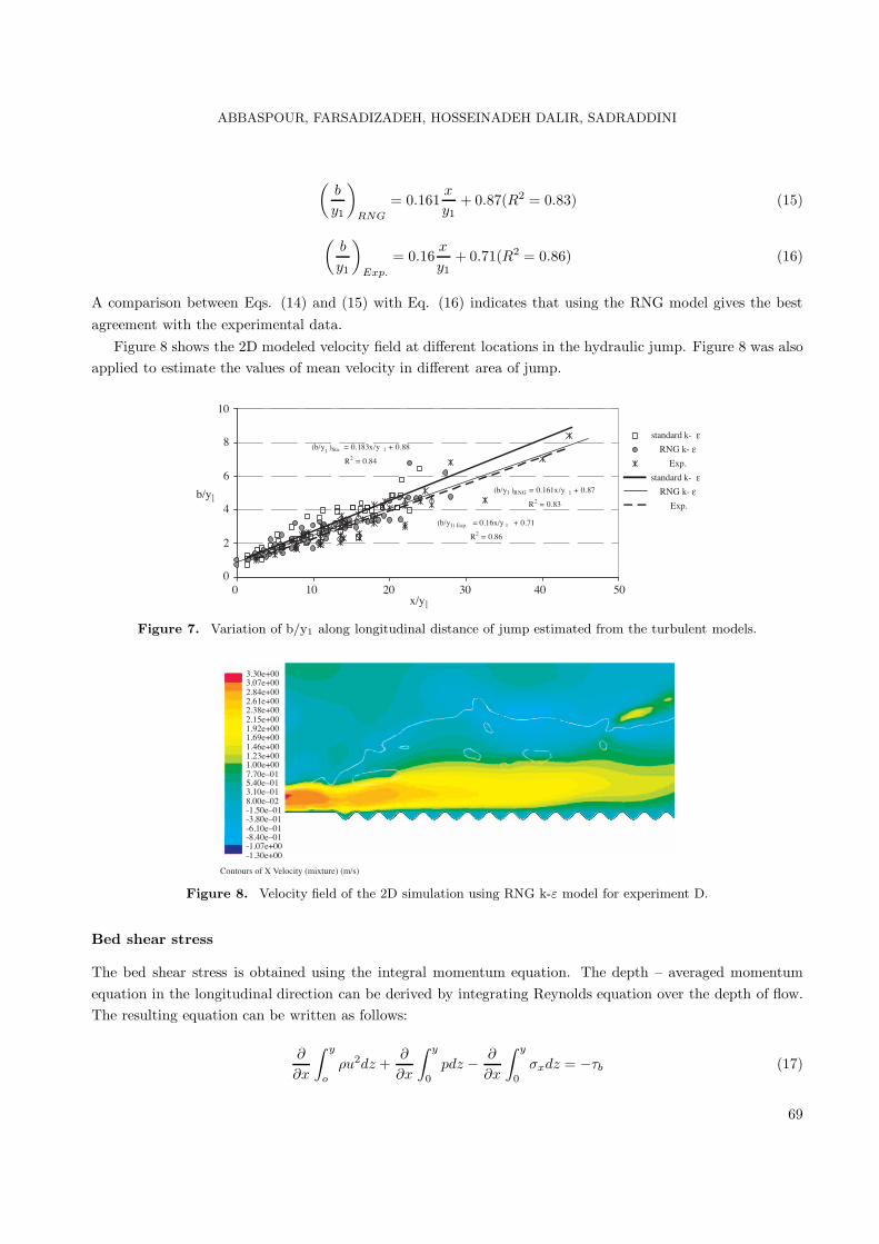
Figure 7 shows the variation of length scale b/y1 with the normalized longitudinal distance x/y1. The linear

relationship between b/y1 and x/y1 for standard k-ε, RNG k-ε models, and experimental data can be describedas the following equations respectively:

(b

y1

)sta.

= 0.183x

y1+ 0.88(R2 = 0.84) (14)

Exp. Data

R2= 0.95

0

0.2

0.4

0.6

0.8

1

0 0.1 0.2 0.3 0.4 0.5 0.6 0.7 0.8 0.9 1x/L

(y-y

1)/(y

2-y1)

Figure 5. Comparison of normalized free surface profiles of jumps on the corrugated bed.

0

0.3

0.6

0.9

1.2

1.5

1.8

0 0.2 0.4 0.6 0.8 1 1.2u/um

u/um u/um

0 0.2 0.4 0.6 0.8 1 1.2u/um

y/b

Exp. Ead &Rajaratnam

Exp. Ead &Rajaratnam

0

0.4

0.8

1.2

1.6

2

0 0.2 0.4 0.6 0.8 1 1.2 0 0.2 0.4 0.6 0.8 1 1.2

y/b

0

0.2

0.4

0.6

0.8

1

1.2

1.4

1.6

0

0.5

1

1.5

2

2.5

y/b

y/b

Exp.Exp.

Exp. B2

Exp. G Exp. D

Exp. C2

Figure 6. Velocity profiles in the forward flow for experiments B2 and C2, D, and G.

68


(b

y1

)RNG

= 0.161x

y1+ 0.87(R2 = 0.83) (15)

(b

y1

)Exp.

= 0.16x

y1+ 0.71(R2 = 0.86) (16)

A comparison between Eqs. (14) and (15) with Eq. (16) indicates that using the RNG model gives the bestagreement with the experimental data.

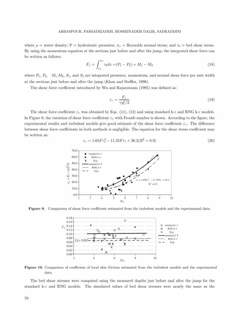
Figure 8 shows the 2D modeled velocity field at different locations in the hydraulic jump. Figure 8 was alsoapplied to estimate the values of mean velocity in different area of jump.

standard k-

RNG k-

Exp.

standard k-

RNG k-

Exp.

(b/y1

)Sta. = 0.183x/y 1 + 0.88

R2 = 0.84

(b/y1 )RNG = 0.161x/y 1 + 0.87

R2 = 0.83

(b/y1) Exp. = 0.16x/y 1 + 0.71

R2 = 0.86

10

8

6

4

2

00 10 20 30 50

x/y140

b/y1

Figure 7. Variation of b/y1 along longitudinal distance of jump estimated from the turbulent models.

2.84e+00

Contours of X Velocity (mixture) (m/s)

3.30e+003.07e+00

-1.30e+00

-8.40e–01-1.07e+00

2.15e+00

2.61e+002.38e+00

1.46e+00

1.92e+001.69e+00

7.70e–01

1.23e+001.00e+00

8.00e–02

5.40e–013.10e–01

-6.10e–01

-1.50e–01-3.80e–01

Figure 8. Velocity field of the 2D simulation using RNG k-ε model for experiment D.

Bed shear stress

The bed shear stress is obtained using the integral momentum equation. The depth – averaged momentumequation in the longitudinal direction can be derived by integrating Reynolds equation over the depth of flow.The resulting equation can be written as follows:

∂

∂x

∫ y

o

ρu2dz +∂

∂x

∫ y

0

pdz − ∂

∂x

∫ y

0

σxdz = −τb (17)

69


where ρ = water density; P = hydrostatic pressures; σx = Reynolds normal stress; and τb = bed shear stress.By using the momentum equation at the sections just before and after the jump, the integrated shear force canbe written as follows:

Fτ =∫ x2

x1

τbdx =(P1 − P2) + M1 − M2 (18)

where P1, P2, M1,M2, S1, and S2 are integrated pressures, momentum, and normal shear force per unit width

at the sections just before and after the jump (Khan and Steffler, 1996).

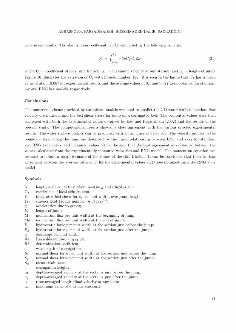
The shear force coefficient introduced by Wu and Rajaratnam (1995) was defined as:

ετ =Fτ

γy21/2

(19)

The shear force coefficient ετ was obtained by Eqs. (11), (12) and using standard k-ε and RNG k-ε models.In Figure 9, the variation of shear force coefficient ετ with Froude number is shown. According to the figure, theexperimental results and turbulent models give good estimate of the shear force coefficient ετ . The differencebetween shear force coefficients in both methods is negligible. The equation for the shear stress coefficient maybe written as:

ετ = 1.65Fr21 − 11.25Fr1 + 26.2(R2 = 0.9) (20)

standard k- ε

RNG k- ε

Exp.standard k- εε

RNG k- ε

Exp.

ετ = 1.65Fr 12

- 11.25Fr 1 + 26.2

R2 = 0.9

0.0

10.0

20.0

30.0

40.0

50.0

60.0

70.0

2 3 4 5 6 7 8 9 10Fr1

ε τ =

Fτ

/(y 1

2 /2)

Figure 9. Comparison of shear force coefficient estimated from the turbulent models and the experimental data.

Cf = 0.067

0.000.020.040.060.080.100.120.140.160.18

2 4 6 8 10Fr1

C fstandard k- ε

RNG k- ε

Exp.standard k- εε

RNG k- ε

Exp.

Figure 10. Comparison of coefficient of local skin friction estimated from the turbulent models and the experimental

data.

The bed shear stresses were computed using the measured depths just before and after the jump for thestandard k-ε and RNG models. The simulated values of bed shear stresses were nearly the same as the

70


experiment results. The skin friction coefficient can be estimated by the following equation:

Fτ =∫ Lj

X=0

0.5ρCfu2mΔx (21)

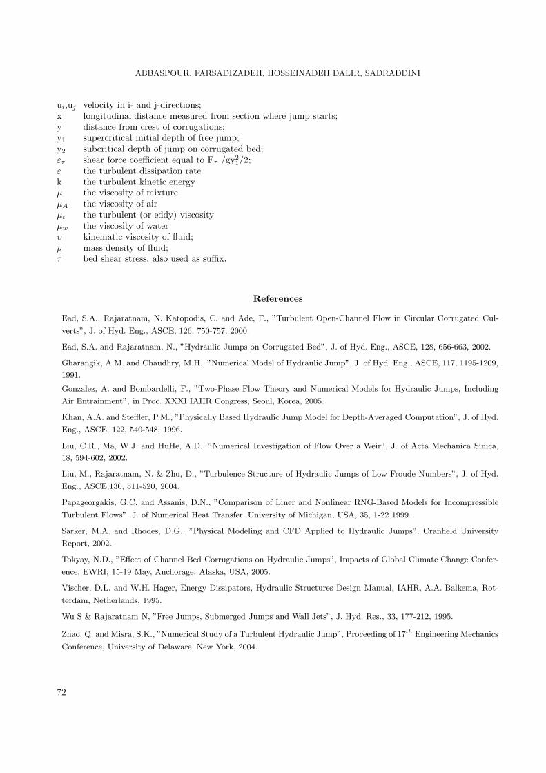
where Cf = coefficient of local skin friction; um = maximum velocity at any station, and Lj = length of jump.

Figure 10 illustrates the variation of Cf with Froude number, Fr1. It is seen in the figure that Cf has a mean

value of about 0.067 for experimental results and the average values of 0.1 and 0.077 were obtained for standardk-ε and RNG k-ε models, respectively.

Conclusions

The numerical scheme provided by turbulence models was used to predict the 2-D water surface location, flowvelocity distribution, and the bed shear stress for jump on a corrugated bed. The computed values were thencompared with both the experimental values obtained by Ead and Rajaratnam (2002) and the results of thepresent study. The computational results showed a close agreement with the various selected experimentalresults. The water surface profiles can be predicted with an accuracy of 1%-8.6%. The velocity profiles in theboundary layer along the jump are described by the linear relationship between b/y1 and x/y1 for standardk-ε, RNG k-ε models, and measured values. It can be seen that the best agreement was obtained between thevalues calculated from the experimentally measured velocities and RNG model. The momentum equation canbe used to obtain a rough estimate of the values of the skin friction. It can be concluded that there is closeagreement between the average value of Cf for the experimental values and those obtained using the RNG k−ε

model.

Symbols

b length scale equal to y where u=0.5um and (du/dy) < 0Cf coefficient of local skin frictionFτ integrated bed shear force, per unit width, over jump length;Fr1 supercritical Froude number=u1/(gy1)0.5;g acceleration due to gravity;Lj length of jump;M1 momentum flux per unit width at the beginning of jump;M2 momentum flux per unit width at the end of jump;P1 hydrostatic force per unit width at the section just before the jump;P2 hydrostatic force per unit width at the section just after the jump;q discharge per unit widthRe Reynolds number= u1y1 /υ;R2 determination coefficient;s wavelength of corrugations;S1 normal shear force per unit width at the section just before the jump;S2 normal shear force per unit width at the section just after the jump;Sij mean strain rate;t corrugation height;u1 depth-averaged velocity at the sections just before the jump;u2 depth-averaged velocity at the sections just after the jump;u time-averaged longitudinal velocity at any point;um maximum value of u at any station x;

71


ui,uj velocity in i- and j-directions;x longitudinal distance measured from section where jump starts;y distance from crest of corrugations;y1 supercritical initial depth of free jump;y2 subcritical depth of jump on corrugated bed;ετ shear force coefficient equal to Fτ /gy2

1/2;ε the turbulent dissipation ratek the turbulent kinetic energyμ the viscosity of mixtureμA the viscosity of airμt the turbulent (or eddy) viscosityμw the viscosity of waterυ kinematic viscosity of fluid;ρ mass density of fluid;τ bed shear stress, also used as suffix.

References

Ead, S.A., Rajaratnam, N. Katopodis, C. and Ade, F., ”Turbulent Open-Channel Flow in Circular Corrugated Cul-

verts”, J. of Hyd. Eng., ASCE, 126, 750-757, 2000.

Ead, S.A. and Rajaratnam, N., ”Hydraulic Jumps on Corrugated Bed”, J. of Hyd. Eng., ASCE, 128, 656-663, 2002.

Gharangik, A.M. and Chaudhry, M.H., ”Numerical Model of Hydraulic Jump”, J. of Hyd. Eng., ASCE, 117, 1195-1209,

1991.

Gonzalez, A. and Bombardelli, F., ”Two-Phase Flow Theory and Numerical Models for Hydraulic Jumps, Including

Air Entrainment”, in Proc. XXXI IAHR Congress, Seoul, Korea, 2005.

Khan, A.A. and Steffler, P.M., ”Physically Based Hydraulic Jump Model for Depth-Averaged Computation”, J. of Hyd.

Eng., ASCE, 122, 540-548, 1996.

Liu, C.R., Ma, W.J. and HuHe, A.D., ”Numerical Investigation of Flow Over a Weir”, J. of Acta Mechanica Sinica,

18, 594-602, 2002.

Liu, M., Rajaratnam, N. & Zhu, D., ”Turbulence Structure of Hydraulic Jumps of Low Froude Numbers”, J. of Hyd.

Eng., ASCE,130, 511-520, 2004.

Papageorgakis, G.C. and Assanis, D.N., ”Comparison of Liner and Nonlinear RNG-Based Models for Incompressible

Turbulent Flows”, J. of Numerical Heat Transfer, University of Michigan, USA, 35, 1-22 1999.

Sarker, M.A. and Rhodes, D.G., ”Physical Modeling and CFD Applied to Hydraulic Jumps”, Cranfield University

Report, 2002.

Tokyay, N.D., ”Effect of Channel Bed Corrugations on Hydraulic Jumps”, Impacts of Global Climate Change Confer-

ence, EWRI, 15-19 May, Anchorage, Alaska, USA, 2005.

Vischer, D.L. and W.H. Hager, Energy Dissipators, Hydraulic Structures Design Manual, IAHR, A.A. Balkema, Rot-

terdam, Netherlands, 1995.

Wu S & Rajaratnam N, ”Free Jumps, Submerged Jumps and Wall Jets”, J. Hyd. Res., 33, 177-212, 1995.

Zhao, Q. and Misra, S.K., ”Numerical Study of a Turbulent Hydraulic Jump”, Proceeding of 17th Engineering Mechanics

Conference, University of Delaware, New York, 2004.

72

numerical study of hydraulic jumps on corrugated beds...

Documents