numerical study of mixing of a supercritical jet in a
TRANSCRIPT

Dissertations and Theses
7-2017
Numerical Study of Mixing of a Supercritical Jet in a Supercritical Numerical Study of Mixing of a Supercritical Jet in a Supercritical
Environment Environment
Neil Sullivan
Follow this and additional works at: https://commons.erau.edu/edt
Part of the Aerospace Engineering Commons
Scholarly Commons Citation Scholarly Commons Citation Sullivan, Neil, "Numerical Study of Mixing of a Supercritical Jet in a Supercritical Environment" (2017). Dissertations and Theses. 376. https://commons.erau.edu/edt/376
This Thesis - Open Access is brought to you for free and open access by Scholarly Commons. It has been accepted for inclusion in Dissertations and Theses by an authorized administrator of Scholarly Commons. For more information, please contact [email protected].

NUMERICAL STUDY OF MIXING OF A SUPERCRITICAL JET IN A
SUPERCRITICAL ENVIRONMENT
A Thesis
Submitted to the Faculty
of
Embry-Riddle Aeronautical University
by
Neil Sullivan
In Partial Fulfillment of the
Requirements for the Degree
of
Master of Science in Aerospace Engineering
July 2017
Embry-Riddle Aeronautical University
Daytona Beach, Florida

NUMERICAL STUDY OF MIXING OF A SUPERCRITICAL JET IN A SUPERCRITICAL ENVIRONMENT
by
Neil Sullivan
A Thesis prepared under the direction of the candidate's committee chairman, Dr. Mark Riddick, Department of Aerospace Engineering, and has been approved by the members of the thesis committee. It was submitted to the School of Graduate Studies and Research
and was accepted in partial fulfillment of the requirements for the degree of Master of Science in Aerospace Engineering.
THESIS COMMITTEE
Member, Dr. Eric Perrell
~11~-Member, Dr. Scott Martin
Date
'7/ i6/ ,7 Date
Date

iii
ACKNOWLEDGMENTS
I would like to first thank my thesis supervisor, Dr. Mark Ricklick for his guidance
and patience, without which this work would not have been possible. Thanks are extended
also to my thesis committee for taking the time to participate and also helping guide the
work.
My new bride is an endless source of love and support. She may roll her eyes or
lose interest when I talk at length or in detail about what I’m doing, but her faith in me is
a large part of what keeps driving me to the finish line. Thanks Laura, and I love you.
I would not be where I am today, either as a student or a man, without the constant
love, encouragement, and support of my late father. The debt owed to him could never be
repaid and it leaves me only with the obligation to work hard, try my best and repeat his
example of generosity and selflessness unto others. Thanks Dad, and I love you.

iv
TABLE OF CONTENTS
LIST OF TABLES ............................................................................................................. vi
LIST OF FIGURES ......................................................................................................... vii
SYMBOLS ......................................................................................................................... ix
ABBREVIATIONS ............................................................................................................ x
ABSTRACT ....................................................................................................................... xi
1. Introduction .......................................................................................................... 1
Turbulent Free Jet ........................................................................................................................... 2
Supercritical Fluids ......................................................................................................................... 4
Applications .................................................................................................................................... 7 Problem Statement ......................................................................................................................... 8
2. Literature Review ............................................................................................... 10
Experiments in Supercritical Jets ................................................................................................ 10
Approaches to Modeling Supercritical Jets ................................................................................ 15 Applications of Supercritical Fluid Modeling ............................................................................ 32
3. Model Setup .................................................................................................... 35
Code, Benchmark and Computational Grid ............................................................................... 35
STAR-CCM+ Coupled Flow Solver .......................................................................................... 39 Reynolds-Averaged Navier-Stokes ............................................................................................. 41 k-Omega SST Turbulence Model ............................................................................................... 41
Large Eddy Simulation ................................................................................................................ 43 NIST REFPROP Data .................................................................................................................. 44
Boundary and Initial Conditions ................................................................................................. 44 Model settings: RANS ................................................................................................................. 46 Model Settings: LES .................................................................................................................... 46
Original Test Case Matrix ............................................................................................................ 47 Challenges with LES and Lessons Learned ............................................................................... 48
Revised Test Case Matrix ............................................................................................................ 48 Grid Independence ....................................................................................................................... 49
4. Results and Discussion ....................................................................................... 54
Preliminaries: First Steps in Benchmarking ............................................................................... 54
LES Results .................................................................................................................................. 61 RANS Results: Comparison with Previous Work ..................................................................... 64 RANS Results: Comparison of Subcritical and Supercritical Results ...................................... 76 Final Thoughts .............................................................................................................................. 79
5. Conclusions and Recommendations .......................................................... 81
Future Work .................................................................................................................................. 82
REFERENCES ................................................................................................................. 84

v
A. Model Convergence Data ................................................................................... 93

vi
LIST OF TABLES
Table 3.1 Experiment Data (Branam, 2002) ..................................................................... 35
Table 3.2 2D Grid Quality ................................................................................................ 37
Table 3.3 3D Grid Quality ................................................................................................ 38
Table 3.4 Inlet Boundary Condition Parameters ............................................................... 45
Table 3.5 Physics Models Used in RANS Simulation ...................................................... 46
Table 3.6 Physics Models Included in LES Simulation ................................................... 47
Table 3.7 Benchmarking Test Matrix ............................................................................... 47
Table 3.8 Nominal Test Matrix ......................................................................................... 48
Table 3.9 Test Case Matrix: Supercritical Jet ................................................................... 49
Table 3.10 Test Case Matrix: Atmospheric Jet, User-Defined EoS ................................. 49
Table 3.11 Test Case Matrix: Atmospheric Jet, Ideal Gas EoS ........................................ 49

vii
LIST OF FIGURES
Figure 1.1 Turbulent Free Jet Streamwise-Direction Mixing Regions (Zong, 2004) ......... 3
Figure 1.2 Turbulent Free Jet Transverse-Direction Mixing Regions (Felouah, 2009) ..... 4
Figure 1.3 P-T Diagram of Supercritical Region for N2 ..................................................... 5
Figure 1.4 Variation in cp with Temperature on a 3.4 MPa Isobar (NIST Chemistry
WebBook) ........................................................................................................................... 6
Figure 3.1 Experimental Setup (Branam, 2002) ............................................................... 36
Figure 3.2 Centerline Density: Unsteady RANS .............................................................. 50
Figure 3.3 Centerline Axial Velocity: Unsteady RANS ................................................... 51
Figure 3.4 Axial Velocity Profiles: Unsteady RANS, Reference Mesh ........................... 52
Figure 3.5 Axial Velocity Profiles: Unsteady RANS, Mesh Level 2 ............................... 52
Figure 3.6 Axial Velocity Profiles: Unsteady RANS, Mesh Level 3 ............................... 53
Figure 4.1 Half-jet velocity contour, reference mesh ....................................................... 55
Figure 4.2 Centerline Density of a 1 atm jet using ideal gas EoS .................................... 55
Figure 4.3 Pressure contour of a steady-state jet .............................................................. 56
Figure 4.4 Density contour of a steady-state jet ............................................................... 56
Figure 4.5 N2 Density Calculation Using PR EoS Compared to NIST Data on a 3.5 MPa
Isobar................................................................................................................................. 57
Figure 4.6 N2 Density Calculation Using PR EoS Compared to NIST Data on a 130 K
Isotherm ............................................................................................................................ 57
Figure 4.7 Percent Error of Density Calculation on an Isobar .......................................... 58
Figure 4.8 Percent Error of Density Calculation on an Isotherm ..................................... 58
Figure 4.9 Centerline Density of a supercritical jet using the PR EoS, constant properties
........................................................................................................................................... 59
Figure 4.10 Centerline Density Comparison to CharLES results ..................................... 60
Figure 4.11 Centerline Density Comparison to CharLES Results, User-Defined EoS .... 61
Figure 4.12 Nikurasde Fully Developed Turbulent Flow Velocity Profile ...................... 62
Figure 4.13 Velocity Magnitude Contour, CharLES Results (Hickey, 2013) .................. 62
Figure 4.14 Velocity Magnitude Contour, LES Results, Current Work ........................... 62
Figure 4.15 Temperature Contour, CharLES Results, (Hickey, 2013) ............................. 63
Figure 4.16 Temperature Contour, LES Results, Current Work ...................................... 63
Figure 4.17 Centerline Density, LES Results, 680 ms Flowtime, Current Work ............. 63
Figure 4.18 Velocity Magnitude Contour, CharLES Results, (Hickey, 2013) ................. 64

viii
Figure 4.19 Velocity Magnitude Contour, RANS Results, Current Work ....................... 64
Figure 4.20 Temperature Contour, CharLES Results, (Hickey 2013) .............................. 65
Figure 4.21 Temperature Contour, RANS Results, Current Work ................................... 65
Figure 4.22 RANS Centerline Density Compared to CharLES Results ........................... 66
Figure 4.23 Centerline Density: Current Work Compared to Case 6 (3.9 MPa, 133 K, 5.4
m/s), (Branam, 2003) ........................................................................................................ 67
Figure 4.24 Potential Core Penetration vs. Density Ratio (Branam, 2003) ...................... 68
Figure 4.25 Axial Velcocity Profiles, Unsteady RANS ................................................... 69
Figure 4.26 Jet Half-Width Locations, Unsteady RANS .................................................. 69
Figure 4.27 Tabular Jet Spreading Angle Data (Branam, 2003) ...................................... 70
Figure 4.28 Shadowgraph Image: Case 3, 4 MPa, 4.9 m/s, 123 K Injected N2 Jet
(Branam, 2002) ................................................................................................................. 71
Figure 4.29 Density Contour (Snapshot) Unsteady RANS, Current Work ...................... 71
Figure 4.30 Streamwise Direction Turbulent Length Scales, Case 3 (Branam, 2002) ..... 72
Figure 4.31 Transverse Direction Turbulent Length Scales, Case 3 (Branam, 2002) ...... 72
Figure 4.32 Integral Length Scales at Various x/D Locations, Unsteady RANS ............. 74
Figure 4.33 Taylor Microscales at Various x/D Locations, Unsteady RANS .................. 74
Figure 4.34 Kolmogorov Microscales at Various x/D Locations, Unsteady RANS ........ 75
Figure 4.35 Calculated Turbulent Length Scales .............................................................. 75
Figure 4.36 Normalized Centerline Density: Supercritical and two Subcritical
Simulations, Unsteady RANS, Current Work .................................................................. 77
Figure 4.37 Centerline Axial Velocity: Supercritical and two Subcritical Simulations,
Unsteady RANS, Current Work ....................................................................................... 78
Figure 4.38 Dynamic Viscosity Profiles at x/D = 10: Supercritical and two Subcritical
Simulations, Unsteady RANS, Current Work .................................................................. 79
Figure 5.1 Residuals, Unsteady RANS, Supercritical ...................................................... 93
Figure 5.2 Monitor of Density at x/D = 10, Unsteady RANS, Supercritical .................... 93
Figure 5.3 Monitor of Surface Average Density, Unsteady RANS, Supercritical ........... 94
Figure 5.4 Residuals, Unsteady RANS, Subcritical ......................................................... 94
Figure 5.5 Surface Average of Density, Unsteady RANS, Subcritical ............................ 95
Figure 5.6 Monitor of Density at 10 Jet Diameters, Unsteady RANS, Subcritical .......... 95
Figure 5.7 Residuals, LES ................................................................................................ 96
Figure 5.8 Monitor of Density at x/D = 10, LES .............................................................. 96
Figure 5.9 Monitor of Surface Average Density, LES ..................................................... 97

ix
SYMBOLS
m mass
u streamwise velocity
cp specific heat at constant pressure [J/kg K]
ρ density [kg/m3]
k thermal conductivity [W/m K]
μ dynamic viscosity [Pa s]
h specific enthalpy [J/kg]
s specific entropy [J/K]
a speed of sound [m/s]
cv specific heat at constant volume [J/kg K]
γ ratio of specific heats, cp/cv
M Mach number, eg. u/a

x
ABBREVIATIONS
SC Supercritical
NIST National Institute of Standards and Technology
RANS Reynolds-Averaged Navier-Stokes
LES Large Eddy Simulation
DLR Deutches Zentrum für Luft und Raumfahrt (German Aerospace Center)
SGS Sub-Grid Scale
EoS Equation of State
ENO Essentially Non-Oscillatory
MUSCL Monotonic Upstream-Centered Scheme for Conservation Laws
SST Menter’s Shear Stress Transport Model

xi
ABSTRACT
Sullivan, Neil MSAE, Embry-Riddle Aeronautical University, July 2017. Mixing of a
Supercritical Jet in a Supercritical Environment.
A numerical simulation campaign is conducted to better elucidate flow physics and
modeling requirements of a supercritical (SC) nitrogen jet injected into a tank of quiescent
SC nitrogen. The goals of this work are twofold: to inform the design of injectors and
combustion chambers for use in the direct-fired supercritical CO2 (s-CO2) power
generation cycle and cryogenic liquid propellant rockets, and to investigate the extent to
which meaningful flow characterization can be achieved with computationally expedient
methods, using commercial software. Reynolds-Averaged Navier-Stokes (RANS) and
Large Eddy Simulation (LES) approaches are used in STAR-CCM+ versions 10.06.010
and 12.02.011. Jet disintegration is evaluated with velocity, density and temperature
profiles, potential core penetration and identification of turbulent length scales. These data
are compared with experimental data and evaluated against other modeling approaches.
Mixing behavior is expected to mimic that of a single-phase jet, and be diffusion-driven,
as there will be no droplet formation in the supercritical phase. Challenges are encountered
in high computational requirements inherent to unsteady LES. Challenges are also
encountered in simulation stability and convergence given large flow gradients near jet
exit, large fluid property gradients near the critical point, and the small length scale of
energetic flow features unique to this high-pressure thermodynamic regime. Simulation
results over-predict core penetration compared to experiment and previous numerical
efforts and show an overall slower transition to ambient conditions. It is shown however
that commercial code can correctly synthesize the overall flow physics and trends of the

xii
single-phase gas jet behavior expected in purely supercritical turbulent mixing flow.
1
1. Introduction
Effort in the study of supercritical fluid phenomena, specifically turbulent mixing
and heat transfer, has become significant in the last 20 years. This owes in part to the
evolution of certain thermo-fluid systems, as operating temperatures and pressures increase
in the continuing quest for efficiency and performance. Important examples include
compression-ignition (diesel) engines, liquid-propellant rocket engines and new-
generation heat exchangers (Roy, 2010). This increase in research can also be attributed to
the increase in worldwide computer power and advances in parallel computing, with the
world’s most powerful supercomputers now exceeding 100 PetaFlops (peak performance
125 PFlops, or 125 x 1015 floating-point operations/sec) (Fu, 2016). Numerical methods
have also matured in this time to take greater advantage of new computing power (Zong,
2004; Barata, 2003; Cutrone, 2006; Kim, 2011). Large Eddy Simulation (LES) and even
Direct Numerical Simulation (DNS) can be brought to bear on increasingly complex flows
and flow phenomena, and Reynolds-Averaged Navier-Stokes simulations can be run by
non-specialists on less expensive computing assets as an integral part of the product design
cycle.
The present work was inspired by an applied design problem in an emerging,
highly-efficient power generation technology. Sandia National Laboratories (SNL) is
currently working on a 10 MW (electric) “s-CO2 Brayton Power Conversion System” as a
system identification prototype in which the working fluid is supercritical carbon dioxide
in a Brayton thermodynamic cycle. It is intended to replace steam Rankine cycles in many
applications and offers advantages in capital cost and thermal efficiency over the older
cycle (Lewis, 2012). The turbulent mixing of a supercritical jet is more relevant to an

2
undertaking at Southwest Research Institute (SWRI), where a novel cycle is being
developed in which combustion occurs inside the supercritical CO2 medium (Brum 2014).
The design of injectors and combustors for such a plant is the motivation for this paper. A
thorough understanding of the flow physics and modeling requirements of a supercritical
jet in a supercritical environment is first necessary, and this is the focus of current work;
future work will involve co-axial fuel/oxidizer injectors and supercritical cross-flow
domains. High-fidelity real-gas combustion modeling tailored to supercritical flows is also
important in reducing development cost and design cycles. The following pages serve to
introduce the reader to the geometry, thermodynamic regime and mixing phenomena of
concern to current work.
Turbulent Free Jet
The round free jet is a canonical flow whose study dates to the beginning of fluid
mechanics as a field of study. 3rd Baron Rayleigh made contributions to turbulent jet
breakup in the late 19th century (Strutt, 1879). A jet is a flow ejected from a nozzle or
orifice at a high speed relative to fluid surrounding it. Round jets and plane jets are well-
studied viscous flow phenomena. A turbulent jet is defined as a jet that is considered
turbulent (depending on normalization of the Reynolds number) at jet exit, and becomes
more turbulent as flow evolves downstream. Figure 1 shows a typical turbulent free jet,
which traditionally has three streamwise regions.

3
Figure 1.1 Turbulent Free Jet Streamwise-Direction Mixing Regions (Zong, 2004)
The region immediately after jet exit is relatively intact, not having begun the
process of disintegration or atomization into surrounding flow. It contains the potential
core, a relatively coherent region of high density that usually includes only injected fluid,
as this is too early in the jet for significant entrainment to occur. Downstream of this is a
transition region where instability and diffusion begin to break up the jet. Injected fluid
mixes with the surrounding fluid and there is an exchange of momentum. Transverse
velocity profiles, as seen above, begin to flatten as the jet spreads and energy is shared.
Various mixing mechanisms can take place in this region including Plateau-Rayleigh
instability (Strutt, 1879), (or Kelvin-Helmholtz instability (Roy, 2010) in the case of a
laminar jet), atomization and molecular diffusion. The jet becomes relatively diffuse
beyond this region and beyond a certain point is described as self-similar. Here, the non-
dimensionalized streamwise velocity profiles no longer change shape in the streamwise

4
direction, and the life of the jet is in a meaningful sense over. Figure 1.2 indicates jet flow
behavior in the transverse direction.
Figure 1.2 Turbulent Free Jet Transverse-Direction Mixing Regions (Felouah, 2009)
Flow in the shear layer and changes in fluid properties in this region are of particular
interest to present work, as the flow features in this area have the greatest impact on jet
disintegration and mixing.
Supercritical Fluids
A supercritical fluid is defined as a fluid at a temperature and pressure above its
critical point. At this point, intermolecular forces become less dominant compared to the
liquid phase, the densities of liquid and gas phases of the fluid are equal, and the two phases
merge (Yang, 2000). Because there is no discrete phase change, there is no latent enthalpy
above the critical point. Additionally, there is no interface between phases, no surface
tension, and thus no droplet formation or spray behavior in turbulent jets. Figure 1.3
illustrates the thermodynamic location of this condition. The red star indicates ambient
chamber conditions for current work (298 K, 4.0 MPa).

5
Figure 1.3 P-T Diagram of Supercritical Region for N2
Because these temperatures and pressures do not exist at Earth’s surface, the
physics of supercritical fluids is not intuitive. SC fluids have liquid-like densities, gas-like
diffusivities, and a litany of other thermodynamic and transport properties become
weighted averages between corresponding saturated liquids and superheated gases (Bellan,
2000). The critical point is defined as a thermodynamic singularity. Here, latent enthalpy
and surface tension approach zero, but specific heat (cp), thermal conductivity (k), and
isentropic compressibility (Z) tend to infinity. The pseudocritical line can be interpreted as
an extension of the saturation line beyond the critical point. While there is no discrete phase
change in the SC region, the pseudocritical line divides where the fluid will assume more
liquid-like and more gas-like properties. For a given pressure, it is located at a temperature

6
where the fluid has maximum cp, and this maximum decays with distance from the critical
point. Thermodynamic and transport properties can vary wildly near the critical point and
in the transcritical regions around the critical temperature and pressure. Figure 1.4 displays
the significant variation in constant pressure specific heat near the critical point.
Figure 1.4 Variation in cp with Temperature on a 3.4 MPa Isobar (NIST Chemistry
WebBook)
This and other fluid properties can vary by orders of magnitude in this region. This
behavior continues on the pseudocritical line, and while values no longer become
arbitrarily large, there is a pronounced peak. This phenomenon is called “enhancement”
and has a profound effect on the energy transport of SC fluids (Kim, 2011). These large
property gradients are a major source of numerical instability (Bellan, 2000). In current
work, the entire experiment and computational domain are at supercritical conditions. The
ambient fluid is at a thermodynamic state inside the supercritical region indicated by a red
star in Figure 1.3, and the injected jet condition is at a location essentially on top of the

7
pseudocritical line at approximately 40 MPa. The injected jet in this case is therefore
subject to significant heat transfer enhancement, and this has a large impact on flow
development, as described in later chapters.
Applications
While some properties of SC fluids create difficulties in experiment and modeling,
fluids at this condition are integral to some thermo-fluid systems, and these same properties
can make them advantageous. Sandia National Laboratories (SNL) propose using
supercritical CO2 (s-CO2) in a Brayton cycle as a highly-efficient means of cooling nuclear
reactors and as a power generation method for many sources (Lewis, 2012). This could
reduce capital cost as compared to a steam Rankine cycle and achieve much higher thermal
efficiency. Work at SWRI is ongoing on a s-CO2 power generation cycle where combustion
occurs inside the supercritical fluid (Brun, 2014). It is referred to as a direct-fire s-CO2
power cycle, and presents many challenges, not the least of which is improving modeling
of turbulent mixing and combustion in a supercritical fluid. As liquid-propellant rocket
engines operate at ever-higher chamber pressures, it is often now the case that a cryogenic
fuel is injected into conditions above the critical point for that fluid. A better understanding
of the fuel-oxidizer mixing mechanisms at these pressures and temperatures is critical to
improving rocket engine design cycle, which has heretofore relied too heavily on the test
stand and trial and error experiments. This work could also contribute to mitigating
combustion instability due to the coupling of flame-acoustics interaction, chemical kinetics
and real fluid effects (Kim, 2011).

8
Problem Statement
With the eventual goal of informing the design of injectors and combustion
chambers for the direct-fired s-CO2 power cycle, the author seeks to identify numerical
modeling requirements capturing all salient flow physics to the injection and turbulent
mixing of a supercritical jet in a supercritical quiescent flow. This work also applies to
improving injectors in liquid propellant rocket engines (Kim, 2011). Results will focus on
jet breakup, potential core penetration and instabilities while attempting to match flow
trends captured in higher-fidelity models. Supercritical results from current work are also
compared to simulated jet behavior at subcritical conditions using the same code to
highlight key differences and modeling challenges.
While high-fidelity and accurate simulation tools are essential in both first-
principles research and product development, there is simultaneously value in low-cost
methods giving representative or even qualitative results. Use of commercially available
software wherever possible can simplify workflow while reducing a very steep learning
curve for design engineers whose expertise in and experience with computational fluid
dynamics may vary. A commercial CFD/Heat Transfer code STAR-CCM+ is used in
conjunction with real-gas properties extracted from the NIST REFPROP library to evaluate
the capability of the code and compare it to both experimental data and numerical results
from sophisticated RANS and LES codes from literature, specifically tuned for simulation
of trans- and supercritical fluids.
RANS simulations are expected to obscure some finer flow features in the shear
layer due to a smearing effect from both Reynolds-averaging and the isotropy assumption
inherent to the eddy-viscosity turbulence model. LES results are expected to provide much

9
flow detail missing in corresponding RANS results, however at significantly increased
computational cost. To test this hypothesis, the following objectives are defined:
1. Compare fluid property modeling approaches for accuracy and cost.
2. Compare modeling approaches (steady RANS, unsteady RANS and LES) for
accuracy and cost.
3. Identify shortcomings in lower-fidelity models.

10
2. Literature Review
A study of the fluid mechanics literature surrounding jets of supercritical fluids
sheds light on an interesting dichotomy. One can apparently take such a canonical flow as
the free round jet, with all its well-studied properties and behavior, and by the mere
application of a few atmospheres of pressure render it scientifically obscure, intuitively
specious, difficult to measure and laborious to simulate. Although crucial to the continued
development of many high-technology applications, the understanding of turbulent mixing
in near- and supercritical free jets is still in an early phase. The following comprises a well-
rounded survey of experimental and numerical efforts to better understand the physics and
behavior of these jets over the last 20 years.
Experiments in Supercritical Jets
Much effort has been undertaken in the last 20 years to study the flow physics of
high-pressure jets. Branam and Mayer in a 2002 paper focus on identifying average length
scales of turbulent flow features of the core flows in co-axial rocket engine injectors. A
series of trans- and supercritical jets of cryogenic nitrogen were injected into a quiescent
tank of room-temperature supercritical nitrogen. Fully turbulent pipe flow is described at
jet exit, with Reynolds numbers ranging from 34,000 to 180,000, based on jet exit velocity
and injector diameter. Jet exit diameter was 2.2 mm and the tank was of sufficient size that
wall effects are neglected in the analysis and the outlet is deemed sufficiently downstream
that it is considered decoupled from the flow field being considered. Walls were heated to
permit a continuous adiabatic wall condition (Branam, 2002). This experimental apparatus
is described in detail because this and other papers use similar or identical setups and/or
data for other studies and to validate models. The shadowgraph technique was used here

11
with a digital camera on the optically-accessible container, after which an algorithm was
used on individual greyscale pixels to obtain average length scale measurements. Turbulent
eddies in the mixing layer are the principal transport mechanisms for mass and energy
transfer, and previous and current work confirm their contribution (Branam, 2002). One of
the most influential parameters on flow development in the jet is the ratio of injected jet
velocity to surrounding fluid velocity, or, in the case of a quiescent environment, ratio of
the density of fluid at jet exit to surrounding fluid density (Branam, 2002, Roy, 2010).
Experimental data were compared with commercial code using k-epsilon turbulence
closure and using real-gas properties. Comparison was then made to the integral length
scale, Taylor microscale, and Kolmogorov microscale. These length scales are described
in equations 1-3 (Branam, 2002).
𝐿𝑖𝑛𝑡 =𝑘
32
휀(1)
𝐿𝑇𝑎𝑦 = (15𝜈��2
휀)
12
, �� = (𝑢2 + 𝑣2 + 𝑤2
3)
12
(2)
𝐿𝐾𝑜𝑙 = (𝜈3
휀)
14
(3)
Where k is turbulent kinetic energy, ε is the turbulent dissipation rate, ν is the
kinematic viscosity, and u, v, and w are generalized basis vector velocities.
In general, observed turbulent flow features, when geometrically averaged,
exhibited length scales with strong correspondence to calculated Taylor microscales, which
are average length scales where the largest amount of energy is dissipated. These tend to
be an order of magnitude larger than Kolmogorov microscales, and an order of magnitude

12
smaller than integral length scales (Branam, 2002).
Further work was done by Branam and Mayer to characterize the high-density core
flow of oxidizer in a co-axial injector, using cryogenic nitrogen to simulate liquid oxygen.
Density, length scales and jet spreading angles are compared for injected nitrogen jets at
several temperatures and injection velocities to evaluate mass mixing and jet dissipation.
Change in temperature of the injected fluid was found to have the largest impact on jet
behavior, as this changes the density ratio between fluid at jet exit and the surroundings
(Branam, 2003). Also of interest in characterizing the jet flow is the axial distance at which
self-similarity is achieved, which is the region where flow properties can be considered
functions of one variable only (axial distance). It is here noted that self-similarity can exist
for one flow property, such as axial velocity, but not for others, such as density or turbulent
kinetic energy (Branam, 2003). In this paper, the self-similar region shall be defined as the
area where axial velocity has become sufficiently diffuse to be considered a function of
axial distance only. Branam and Mayer here compare the same experimental data as before
against a Favre-Averaged Navier-Stokes (FANS) commercial code with k-epsilon
turbulence closure called CFD-ACE. Real gas models are invoked here, namely Lee-
Kesler, Chung et al and a modified version of Benedic-Webb-Rubin equation of state. This
code can resolve weak compressibility effects by virtue of real gas relationships for density,
specific heat, viscosity and thermal conductivity which are derived from the above EoS
(Branam, 2003). The result is an incompressible, yet variable-density code, suitable for low
Mach numbers, and incorporating variable isentropic compressibility. Calculated Grashof,
Froude and Reynolds numbers indicate that inertial forces are significant while body forces
and buoyancy, as well as viscous forces can be neglected (Branam, 2003). This supports

13
the contention that supercritical jet mixing is primarily diffusion-driven, and will be similar
qualitatively to single-phase gas-gas mixing. Several metrics including radial property
profiles, centerline density, potential core length and jet divergence angle are compared to
present work.
Polikhov, in a 2007 paper, presents an experiment using planar laser induced
fluorescence (PLIF) to generate a section through the jet center, in hopes of eliminating
some shortcomings inherent to shadowgraphy, used to produce most data in previous work
on supercritical jet mixing (Polikhov, 2007). Principal issues with the shadowgraph
technique are two-fold. It is an integrative observation technique, in that light entering the
camera must pass through the entire jet, such that the measurement taken is an average.
Secondly, the technique measures density gradient, and not an absolute density. This means
low-density but highly turbulent regions can saturate the image. These regions of low-
density mixed fluid can suggest highly-diffuse gas-gas like mixing, while potentially
obscuring a high-density core at the jet center (Polikhov, 2007). A cryogenic fluid, FK-5-
1-12, is injected into a chamber filled with nitrogen at varying conditions: subcritical,
transcritical and supercritical, with respect to the injected fluid. A linear stability analysis
is performed to develop a distortion relation for the viscous jet in inviscid gaseous
surroundings. This is successful for the subcritical case, but fails as temperature and
pressure are raised in the container. Large density gradient between injected and
surrounding fluid is found to have a damping effect on turbulence, and decreases the
mixing rate. This leads to a longer potential core length.
Studies of free jets of course date back to the origins of fluid mechanics, with
notable efforts by Rayleigh and Prandtl when the field of turbulent mixing was in its

14
infancy (Roy, 2010). Many semi-empirical expressions exist for subcritical jet breakup
length and droplet size distribution for two-phase flows, but these types of qualifications
are lacking in the literature for trans- and supercritical flows (Roy, 2010). The author notes
that Kelvin-Helmholtz instabilities (KHI) can describe the breakup of an initially laminar
jet, but this theory does not apply to the breakup and atomization of an initially turbulent
jet (Roy, 2010).
Roy and Segal employ a novel method of fluorescing Perfluoroketone, a 3M
product, to detect detailed structures in a jet center plane, and study flow-field densities.
This jet flow is important to drive design of future liquid-propellant rocket engines as well
as pressure-ignition reciprocating engines, where liquid fuels are injected into supercritical
conditions relative to the fuel. Density gradient profiles were generated and potential core
lengths measured, which were then compared to previous flow visualization results. Three
major cases were studied: a subcritical jet into a subcritical environment, a subcritical jet
into a supercritical environment (relative to the injected fluid), and a supercritical jet
injected into a supercritical environment. Chamber/injected fluid density ratios ranged
from 0.01 to 0.04. In the trans- and supercritical regime, this pressure ratio is found to be a
strong driver of flow development and potential core length, whereas this strong
correspondence is not encountered in subcritical single-phase gas jets. Core lengths were
evaluated by algorithms using the extracted optical data, and an eigenvalue approach was
taken to determine the location of maximum density gradients. The literature does not
contain a unique, precise definition of the potential core of supercritical jets, and here it is
taken as an intact region of higher density than downstream areas. In the supercritical
jet/supercritical chamber case, potential core length was shorter than in the either

15
subcritical case, and this is attributed to the aforementioned density ratio. As temperature
and pressure in the chamber increase, jet mixing qualitatively approaches single-phase gas-
gas, as the density ratio will decrease, and so will the stabilizing effect of a high radial
density gradient. Shear layer instabilities were low, smoothing the jet at the supercritical
condition, and this trend continued as density gradient values decreased downstream.
Mixing phenomena when injected fuel is supercritical but surrounding environment
is subcritical relative to the fuel are less covered in the literature but are treated from the
perspective of supersonic combustor (scramjet) design by Wu in a 1999 paper. Wu studies
under-expanded supersonic supercritical ethylene jets entering a superheated combustion
chamber, measuring the location and size of Mach discs (shock diamonds) and jet
expansion angle. Schlieren photography and Raman scattering techniques are used in this
experiment. Fuel is intended to act as a heat sink to modulate fuselage temperatures at
hypersonic vehicle velocities, and may go beyond its critical point before it is injected into
the combustor (Wu, 1999). Mixing was determined by fuel mole fraction and temperature
distributions. As the injected jet initial condition approached the critical point, ethylene
centerline mole fraction increased, as did the jet width at a location of stoichiometric
mixture. Temperature deficit in the jet was also more pronounced at near-critical
conditions. This suggests turbulent mixing was inhibited in the trans-critical regime. Mach
disk location was unchanged in a supercritical jet, but expansion angle increased as injected
jet temperature reached the critical temperature (Wu, 1999).
Approaches to Modeling Supercritical Jets
Zong identifies several phenomena compounding existing modeling difficulties
surrounding high-pressure flow in his 2004 paper. Compressibility effects (pressure-

16
induced volumetric changes) and variable inertia effects (resulting from heat addition or
variable composition in chemically reacting flows) can lead to instability. Additionally, as
density increases, so does Reynolds number (Re increases approximately linearly with
pressure) which tends to shrink Taylor and Kolmogorov microscales (Zong, 2004). This in
turn requires mesh refinement to capture flow features carrying a large portion of the
energy spectrum.
Zong conducts a LES study on subcritical liquid nitrogen injection into a
supercritical environment using full conservation laws and real-fluid thermodynamics and
transport phenomena. A modified form of the Soave-Redlick-Kwong (SRK) cubic
equation of state (EoS) is used. The real-gas properties are calculated with departure
functions, which constitute the sum of an ideal gas contribution with a real-gas effect near
the critical point. The modified SRK and example internal energy departure function are
presented as equations 4 and 5.
𝑃 =𝜌𝑅𝑢𝑇
𝑊 − 𝑏𝜌−
𝑎𝛼
𝑊
𝜌2
(𝑊 + 𝑏𝜌)(4)
𝑒(𝑇, 𝜌) = 𝑒0(𝑇) + ∫ [𝑃
𝜌2−
𝑇
𝜌2(𝜕𝑃
𝜕𝑇)𝜌]𝑇
𝜌
𝜌0
𝜕𝜌 (5)
Where P is pressure; ρ is density; Ru is the universal gas constant; T is temperature;
W is a model parameter arising from SRK modification; a and b are other model
parameters; and α is a parameter containing an approximated critical compressibility factor
and the acentric factor, a molecular property.
A preconditioning scheme is employed here to offset the stiff matrix problem
inherent to modeling supercritical fluids (Zong, 2004; Weiss, 1995). This code’s solver is
4th-order centered in space and 2nd-order backward-difference in time, with a 3rd-order

17
Runge-Kutta scheme used in the pseudo-time preconditioning inner loop. The domain is a
modest 225x90 point structured grid, with a fully-developed turbulent pipe flow inlet. Zong
states that a single-phase jet shear layer has KH instabilities (for a certain Reynolds number
range) and vortex rolling, pairing, and breakup. A cryogenic supercritical jet has these
features and adds additional mechanisms due to baroclinic torque (a moment resulting from
misalignment of a density gradient and a pressure gradient) and the volumetric changes
described above. Zong’s contention that a strong pressure gradient at the injector has a
stabilizing effect on flow development is in keeping with the literature. The spatial growth
rate of surface instability waves increases with increasing ambient pressure, or decreasing
pressure ratios (which couple to density ratios). An increase in ambient pressure also leads
to an earlier transition to self-similarity (Zong, 2004). Characteristic times did not change
at supercritical conditions. Drastic changes in jet surface phenomena are noted across the
critical pressure, and above the critical point, the jet surface topology mirrors a submerged
gaseous jet, with spatial growth rate mimicking an incompressible but variable-density gas
jet. At high pressure ratios, high density gradient regions develop around the jet surface
due to intensive property variations. This acts as a solid wall which amplifies axial flow
oscillations but damps radial oscillations. In this way instability in the shear layer is
reduced. This damping effect decreases with decreasing pressure ratio, causing the jet to
expand more rapidly at higher ambient pressure.
In a 2000 critical review, Bellan focuses on differentiating subcritical and
supercritical flow turbulent mixing behavior and establishes a more accurate generalized
nomenclature appropriate for all thermodynamic states. She characterizes the SC state by
the “impossibility of a two-phase region” (Bellan, 2000). The high solubility of SC fluids

18
becomes important to mixing, both with other supercritical fluids and other solutes, as does
the heat of solvation. These properties will vary near the critical point given their sensitivity
to density and in turn the sensitivity of density to temperature and pressure. Heat of
solvation becomes an important thermodynamic quantity indicative of fluid
interpenetration (Bellan, 2000). Complexity arises in the mixing of several near-critical or
SC fluids, as the critical locus, the averaged critical point for the mixture based on
participating species’ mole fractions and thermodynamic state, is not straightforward. It
can be non-monotonic and convoluted depending on mixture species, which is an
additional modeling concern as well as a concern during experiment. As species
concentrations evolve downstream, either by diffusion or chemistry, SC regions may
become subcritical and vice-versa (Bellan, 2000). It is difficult, except in a broad
qualitative sense, to predetermine this mixture behavior.
It has been reasonably established in literature that spreading angle is affected by
chamber/jet density ratio, and the resulting change in fluid entrainment will impact shear
layer evolution. Atomization theories based on Rayleigh-Taylor instabilities (RTI) do not
apply in the SC regime as there is no surface tension. Fluid mixing is instead due to high
turbulence and is molecular diffusion-driven (Bellan, 2000). In a subcritical two-phase
flow, waves form at the surface of the jet (KHI or other instability, depending on Reynolds
number) due to the relative velocity of liquid jet and gas surroundings. The liquid sheet
breaks up and atomizes. However, as ambient conditions approach supercritical relative to
the jet fluid, optical data show “wispy threads” of fluid emerging from the jet wall and
dissolving into the surrounding fluid (Bellan, 2000).
Although it is well-understood that liquid drops (or indeed a full two-phase spray)

19
cannot exist in a thoroughly supercritical flow, owing to the absence of any fluid interface,
jets will still disintegrate. These fluid “chunks” will often travel in the midst of a large
density gradient over their residence time, giving the appearance of an interface in optical
data, obscuring their true nature. Foreknowledge of properties like this is essential to the
experimentalist and modeler. Furthermore, Bellan stresses the importance of consistent
terminology in describing the mixing of SC jets to avoid confusion between researchers
and the readership. Evaporation refers to a strictly subcritical phenomenon where heat is
added to a liquid droplet and mass is transferred across a tangible phase boundary into a
surrounding gas. This is not possible at the SC condition, so rather the process of a “chunk”
of high density SC fluid diffusing into a surrounding region is termed emission. Similarly,
as sprays are also a subcritical phenomenon, a purely SC jet cannot undergo atomization.
Such jets as said to disintegrate into chunks of SC fluid, after which further diffusion can
occur (Bellan, 2000).
Bellan comments on two late 20th century experiments. An Army Research
Laboratory (ARL) study measured a cryogenic jet injected into a supercritical chamber.
The potential core of the methyl iodine jet was not well-defined by established
density/coherence measurements and instead was defined only as a region with high
concentration of injected fluid (Birk, 1995). Increased core penetration was found with
increasing chamber pressure, consistent with results from literature. Here, this was
speculatively attributed to injected fluid reaching critical temperature close to jet exit,
inhibiting jet disintegration and lengthening the core. A study performed at the Air Force
Research Laboratory (AFRL) investigated visual characteristics of round jets of nitrogen,
helium and oxygen in subcritical and supercritical environments. A correlation was found

20
again between chamber/jet density ratio and jet disintegration and spatial evolution. In this
experiment, however, the potential core was shown to become shorter and thinner with
increasing chamber pressure, in contradiction to Birk et al. and many other observations
from literature (Chehroudi, 1999). Bellan offers that this can be explained by a large
temperature difference and therefore overall density difference between the ARL and
AFRL experiments.
Commentary is also offered on numerical modeling efforts. Oefelein and Yang
performed a LES study of LOX and H2 shear layer combustion which employed a
correlation for mass diffusivity between the liquid and gas states to come to a suitable SC
value, however their method did not ensure this value reaches the proper zero value
(another example of the thermodynamic singularity) at the critical point (Oefelein, 1998).
Miller et al., in a DNS study developed a new sub-grid scale (SGS) turbulence model
particularly suited to supercritical flows for future LES. This is important work as existing
SGS models and RANS turbulence transport models were developed with subcritical fluids
in mind (Miller, 2001). A steady-state, 2-D RANS simulation using k-epsilon closure and
real-gas EoS and fluid properties was conducted by Ivancic et al., on combustion of a LOX
jet into hydrogen at 6 MPa. The simulation predicted incorrect thickness and location of
the OH species region, and Bellan attributes this to the significant simplifying assumptions
in the model (steady and 2-dimensional in particular). SC fluids models must be transient,
as the literature shows SC flow behavior is inherently unsteady (Bellan, 2000). A proper
model is time-domain, has a real-gas EoS, and accounts for mixture non-ideality, increased
solubility and Soret and Dufour effects. Numerical codes and models typically used to
simulate jets and shear flows contain turbulence models, which were developed and tuned

21
for subcritical (and in many cases ideal) flows. Numerical tools remain lacking in this
regard. Further, there is need for species-specific thermal diffusion factors (capturing Soret
effect), multi-component mass diffusivities (capturing Dufour effect) and custom
supercritically-based turbulence models (Bellan, 2000).
Vigor Yang contributes a review of modeling aspects in SC vaporization, mixing
and combustion in liquid rockets. He immediately points out that in this regime, the already
difficult problem of determining physical and chemical mechanisms in multiphase,
chemically reacting flows is exacerbated by the inherent increase of Reynolds number
accompanying very high operating pressure. Challenges also arise near the mixture critical
point, as reported elsewhere in literature. Flow behavior in rocket engines is affected by
two phenomena driving volumetric non-idealities: compressibility effects from pressure
changes near the critical point and variable inertia effects from changes in chemical
composition and heat addition, the latter effect being a product of the chemistry in the
combustion chamber. Physical and chemical processes that result from the coupling of fluid
dynamics, heat transfer, chemical kinetics, and thermodynamic and transport non-idealities
have a wide range of time and length scales. Some of these scales are smaller than can be
reasonably resolved numerically (Yang, 2000). The increased Reynolds number due to
high pressure shrinks the scales of SGS phenomena.
Support is shown in this paper for a version of the Benedict-Webb-Rubin (BWR)
cubic EoS modified by Jacobsen and Stewart, and its superior accuracy is compared to the
conventional cubic real-gas equations (Benedict, 1940; Jacobsen, 1973; Yang, 2000). One
drawback of using this high-fidelity equation is that model constants are only available for
a small number of pure substances. An Extended-Corresponding-State (ECS) principle

22
developed by Ely and Hanley can be used to obtain transport properties, using BWR, of
other single-phase fluids by conformal mapping temperature and density to that of a known
reference fluid (Ely, 1981). This means constants are only required for the reference fluid.
The BWR EoS is applied to the reference fluid in equation 6.
𝑃0(𝑇, 𝜌) = ∑ 𝑎𝑛(𝑇)𝜌𝑛
9
𝑛=1
+ ∑ 𝑎𝑛(𝑇)𝜌2𝑛−17𝑒−𝛾𝜌2
15
𝑛=10
(6)
Where P0 is pressure of the reference fluid; T is temperature; ρ is density; γ is 0.04;
and temperature coefficients an(T) depend on the reference fluid. There are 15 temperature
coefficients in this case.
Viscosity and thermal conductivity of mixtures can be obtained using ECS, as
shown in equation 7.
𝜇𝑚(𝜌, 𝑇) = 𝜇0(𝜌0, 𝑇0)𝐹𝜇 (7)
Where μm is dynamic viscosity of the mixture; the subscript 0 indicates properties
of a reference fluid, and Fμ is the mapping function. It is worth noting that the ECS method
cannot account for the contribution of molecular internal degrees of freedom in the
calculation of thermal conductivity, and this term must be provided by a semi-empirical
rule.
Yang demonstrates calculation of the thermodynamic properties with departure
functions, as described by Branam, above. This method can potentially mitigate some of
the complexity in modeling supercritical mixtures, by treating them in some respects as
homogeneous “pseudo-pure” substances. Yang compares density calculations of several
cubic EoS to experimental data from 70 to 430 K and 1-400 atmospheres. Peng-Robinson

23
gave a maximum relative error of 17%, SRK gave a maximum error of 13%, and the
modified BWR gave a maximum error of 1.5% in this region. The BWR EoS must be
solved iteratively for density at given pressure and temperature, increasing computational
cost when used in density-based solvers. However, given its applicability to a large range
of thermodynamic states and improved accuracy relative to other real-gas EoS, it remains
valuable (Yang, 2000).
Barata also comments on a trend of increasing operating pressure in liquid-fueled
rocket combustion chambers. In many engines, the fuel is injected into a chamber above
the fuel’s critical point, presenting design and analysis challenges that arise from a dearth
of knowledge of supercritical turbulent jet mixing. The solubility of the gas phase in the
liquid phase increases as chamber pressure approaches the critical value, while
simultaneously, mixture effects need to be considered in calculating a mixture’s critical
point (Barata, 2003). According to Barata et al., Raman scattering studies demonstrate the
biggest driver of jet growth is the thermodynamic state of the injected fluid, rather than jet
speed. Jets in supercritical media have the same appearance as a gas jet, with a growth rate
mirroring that of an incompressible, variable-density (low Mach numbers) jet.
A 2-D axisymmetric, steady, Favre-Averaged Navier-Stokes (FANS) study using
k-epsilon closure was conducted on a cryogenic liquid jet injected into a chamber at
supercritical temperature relative to the injected fluid. Favre averaging was used to obtain
mass-averaged quantities in the conservation equations. This prevents the inclusion of
terms involving density fluctuations, and reduces the number of models needed to solve
the flow. Equation 8 shows a mass-averaged quantity obtained using Favre averaging, and
momentum and continuity equations are presented in cylindrical polar coordinates for this

24
example, in equations 8-11.
�� =𝜌𝜙
��
(8)
Where the overbar indicates an average given by the Reynolds decomposition.
𝜕��𝑈��
𝜕𝑥+
1
𝑟
𝜕𝑟��𝑈��
𝜕𝑟= −
𝜕��
𝜕𝑥−
1
𝑟
𝜕𝑟��𝑢′′𝑣′′
𝜕𝑟(9)
𝜕��𝑈��
𝜕𝑥+
1
𝑟
𝜕𝑟��𝑉��
𝜕𝑟= −
𝜕��
𝜕𝑥−
1
𝑟
𝜕𝑟��𝑣′′𝑣′′
𝜕𝑟+ ��
𝑤′′𝑤′′
𝑟(10)
𝜕����
𝜕𝑥+
1
𝑟
𝜕𝑟����
𝜕𝑟= 0 (11)
Where the tilde (~) overbar indicates a Favre decomposition, a straight overbar
indicates a Reynolds decomposition, and a double overbar indicates a Favre decomposition
of a Reynolds decomposition.
The authors note the code used was not written specifically for supercritical fluids,
and care was taken to avoid numerical oscillations and divergence due to large density
gradients. Several grids were tested, and high under-relaxation was used for the momentum
equations (up to 90%). To best approximate the experimental conditions, a free-boundary
was used for the wall on either side of the jet exit by setting constant pressure and obtaining
velocity components from the continuity and momentum equations. This also required high
under-relaxation to avoid divergence (Barata, 2003). Uniform axial velocity and zero radial
velocity was set at jet exit, with 0.1% turbulence intensity and turbulent length scale equal
to the initial jet diameter. Variation of turbulence parameters did not significantly impact
flow development due to the uniform inlet velocity profile. Grid independence was
evaluated by axial velocity decay.
Barata et al. compare results from this simulation to data from the Chehroudi 1999

25
paper suggesting gas jet-like behavior, as the code in this case was originally written for
gaseous variable-density flows, and not supercritical flows (Barata, 2003). Potential core
penetration was shown to decrease with increasing chamber pressure, matching
Chehroudi’s observations, and contradicting many others. Self-similarity is achieved
between 8 and 12 jet diameters downstream, and otherwise the model reproduces most
observations referenced previously, including growth rate and similarity in appearance to
gaseous variable-density jets. These results give the authors confidence that a supercritical
jet that looks like a gaseous jet can be modeled as one.
This paper takes a robust approach to modeling near-critical mixing and
combustion, developing a holistic treatment of salient flow physics uniquely suited to SC
flow. This is an unsteady RANS study using k-omega closure. Equations 12 and 13
represent the governing equations in conserved form.
𝜕𝑄
𝜕𝑡+
𝜕𝐸 − 𝐸𝑣
𝜕𝑥+
𝜕𝐹 − 𝐹𝑣
𝜕𝑦= 𝑆 (12)
𝑄 = (��, ����, ����, ����, ��𝑘, ��𝜔, ����𝑖) (13)
Where Q is the vector of conserved variables; �� is density; �� and �� are velocities;
�� is total enthalpy; k is turbulent kinetic energy and ω is its specific dissipation rate; and
𝑌�� is the mass fraction of species i. E, Ev, F, and Fv are the inviscid and viscous flux vectors.
A modified version of the Peng-Robinson (PR) EoS is used for its wide range of
applicability. The PR EoS is shown in equations 14-19 and is used later in this paper.
𝑃 =𝑅𝑢𝑇
𝑉𝑚 − 𝑏−
𝑎𝛼
(𝑉𝑚2 + 2𝑉𝑚𝑏 − 𝑏2)
(14)

26
𝑎 =0.45724𝑅𝑢
2𝑇𝑐2
𝑃𝑐
(15)
𝑏 =0.07780𝑅𝑇𝑐
𝑃𝑐
(16)
𝛼 = {1 + 𝜅(1 − 𝑇𝑟
0.5)}2 (17)
𝜅 = 0.37464 + 1.54226𝜔 − 0.26992𝜔2 (18)
𝑇𝑟 =𝑇
𝑇𝑐
(19)
Where P is pressure; Ru is the universal gas constant; Vm is molar volume; ω is the
acentric factor, a property of molecule geometry; and Tc is the critical temperature and Tr
temperature non-dimensionalized with respect to critical temperature, and referred to as
reduced temperature.
The EoS is presented in polynomial (cubic) form in equations 20-22.
𝐴 =𝑎𝛼𝑃
𝑅𝑢2𝑇2
(20)
𝐵 =𝑏𝑃
𝑅𝑢𝑇(21)
𝑍3 − (1 − 𝐵)𝑍2 + (𝐴 − 2𝐵 − 3𝐵2)𝑍 − (𝐴𝐵 − 𝐵2 − 𝐵3) = 0 (22)
Where Z is isentropic compressibility (Peng, 1975). A mixing rule proposed in
(Miller, 2001) extends the above original form of the PR EoS to treat mixtures. This
modified EoS is used to derive analytical expressions of thermodynamic quantities.
Dynamic viscosity is computed by a two-equation method proposed by (Chung, 1984) and
the ECS method of Ely and Hanley covered above was used to calculate thermal
conductivity, using methane as the reference fluid (Cutrone, 2006). The authors discuss

27
two problems affecting convergence of time-marching schemes used in low speed flows.
The first is machine round-off can cause floating point errors during calculation of the
pressure gradient in the momentum equation. This can be solved by decomposing pressure
into a constant and varying component, as with other variables. The second is the numerical
stiffness of the governing partial differential equations. This can be improved by using a
preconditioning matrix on the RANS equations in pseudotime, improving both
convergence and stability (Cutrone, 2006). Cases are run on a 30,000 point grid, with a
calculated y+ of 1 at the walls.
This robust numerical treatment is first compared against the cold-flow case
presented in (Branam, 2002) and compared well, using radial density profiles at 5 and 25
jet diameters. Such a mono-phase modeling approach is deemed suitable for a wide range
of pressures and temperatures in the near- and supercritical regimes.
As chamber pressure exceeds its critical value, atomization no longer occurs, and
as the fluid in the jet shear layer exceeds its critical temperature, inter-molecular forces
reduce significantly. Diffusion-driven mixing mechanisms are promoted before
atomization can take place, and the jet diffuses in a gas-like manner into the surrounding
fluid. The result is a continuous fluid featuring no interface, but regardless possessing a
very steep gradient of fluid properties in the radial direction (Cutrone, 2006). The injected
cryogenic jet behaves optically like a single-phase gas jet rather than a liquid spray.
A transient RANS code is developed to study the turbulent mixing and combustion
of cryogenic liquid nitrogen jets injected in a supercritical nitrogen chamber. Turbulence
is captured by a modified k-epsilon model, and two real-gas EoS are used and compared.
Real-gas thermodynamic properties are calculated using a dense fluid correction to an ideal

28
gas solution, similar to the departure functions mentioned previously. The method
proposed in (Chung, 1984) is used to calculate dynamic viscosity and thermal conductivity.
As this code is intended to model combustion as well as mixing, binary mass diffusion
coefficients are first estimated for the low-pressure condition per a standard empirically
correlated model in (Fuller, 1966) and high-pressure correction terms are added per
(Takahashi, 1974). Although this added step will contribute to real-gas fidelity, modeling
of the mass diffusion coefficients is still difficult for lack experimental data (Kim, 2011).
Combustion is not treated in present work, and no further detail is provided on the
combustion model. The extended k-epsilon turbulence model is seen in equations 23-25.
𝜕
𝜕𝑡(����) +
𝜕
𝜕𝑥𝑗(����𝑗��) =
𝜕
𝜕𝑥𝑗(𝜇𝑒𝑓𝑓
𝜎𝑘
𝜕��
𝜕𝑥𝑗) + 𝑃𝑘 − ��휀 (23)
𝜕
𝜕𝑡(��휀) +
𝜕
𝜕𝑥𝑗(����𝑗휀) =
𝜕
𝜕𝑥𝑗(𝜇𝑒𝑓𝑓
𝜎𝜀
𝜕휀
𝜕𝑥𝑗) +
휀
��(𝐶𝜀1𝑃𝑘 − 𝐶𝜀2��휀) (24)
𝑃𝑘 = −��𝑢𝑖
′′𝑢𝑗′′ 𝜕��𝑖
𝜕𝑥𝑗
(25)
Where k is turbulent kinetic energy; ε is dissipation rate of turbulent energy; μeff is
effective dynamic viscosity; σk, σε, Cε1 and Cε2 are model constants; and Pk is the
production rate of turbulent energy (Kim, 2011). This varies from the standard k-epsilon
model in use of effective viscosity in place of turbulent viscosity, and use of a unique pre-
calculation method, described below. Turbulent Prandtl number is 0.7 for this model.
A novel approach to decomposition is taken by Kim et al. in the use of a conserved
scalar in concert with a presumed probability density function (PDF). Because the cold-
flow case being tested here is chemically homogeneous and Mach number is low, the
conserved scalar function is normalized static enthalpy. Every Favre-averaged scalar in the

29
solution vector is calculated by integrating the pre-calculation solution in conserved scalar
domain, while weighted with a presumed beta PDF. These elements are shown in equations
26 and 27.
𝑍 =ℎ − ℎ𝑖𝑛𝑗
ℎ𝑚𝑎𝑥 − ℎ𝑖𝑛𝑗
(26)
��(��) = ∫ ��1
0
(𝑍; ��)𝜙(𝑍)𝑑𝑍 (27)
Where Z is the conserved scalar; hmax is the maximum constant static enthalpy, in
this case at an isothermally heated wall; hinj is the minimum value of enthalpy at jet exit; φ
is a thermodynamic or transport property contained in the governing equations; and �� is a
beta PDF. This method is used to represent scalar fluctuation effects on the real fluids in
turbulent mixing near the critical point (Kim, 2011). PR and SRK model predictions are
compared with NIST data for cp and density. PR is found more accurate at predicting jet
density profiles. These models were chosen for their accuracy for low-carbon fuels.
Supercritical fluids have thermodynamic and transport properties in between those
of a liquid at the same pressure and a gas at the same temperature. The solubility is gas-
like, and a strong function of pressure. Density and thermal diffusivity, however, are liquid-
like, and strong functions of temperature (Kim, 2011). The supercritical combustion of
cryogenic liquid propellants is tied to turbulent diffusion. Kim et al. identify the (many)
important physical processes at play in high-pressure liquid propellant combustion:
injection, real fluid effects, turbulent mixing, chemical kinetics, turbulence-chemistry
interaction, flame-acoustics interaction and heat transfer (Kim, 2011). All are highly
complex and all are in some way coupled with one another. Pseudoboiling was observed
in model results. This occurs as heat is added to the inject SC fluid while near the

30
pseudocritical point. It is a point of heat transfer enhancement, as it is the temperature at
which cp and Z (isentropic compressibility) are maximum for a given pressure. Heat
addition at this point will promote a relatively small increase in temperature, but a relatively
large increase in specific volume (Kim, 2011). The test matrix transited the critical and
pseudocritical points, and were therefore well-suited to validate the model. The pseudo-
boiling phenomena had significant impact on flow development, and it was shown that
strong pseudo-boiling increases the core penetration length and slows axial velocity decay.
The paper identifies a need for a comprehensive modeling approach to reduce the
design-cycle cost for liquid-propellant rocket engines, as the industry’s significant reliance
on trial-and-error methods is expensive and time-consuming.
In a 2013 paper, Hickey and Ihme evaluate the capabilities of CharLESx, a cleverly-
named LES solver developed at Stanford University’s Center for Turbulence Research and
now sold by Cascade Technologies, a spin-off of the CTR. Motivation for this work is to
test real-fluid extensions to the code, and a desire to model mixing and combustion in liquid
rocket engines where injected fuel and oxidizer become supercritical during combustion.
It is believed better modeling tools are key to predicting combustion instability (Hickey,
2003).
CharLESx is an unstructured LES code, using a 3rd-order Runge-Kutta explicit
solver in time and a hybrid 4th-order centered solver in space. The space-domain solver
uses a density gradient trigger to switch to a 1st- or 2nd-order Essentially Non-Oscillatory
(ENO) solver if gradient passes through a preset threshold. This mitigates numerical
dissipation and convergence issues for flow solutions that may contain large gradients,
shocks or other discontinuities. The SGS model is an eddy-viscosity model developed for

31
turbulent shear flow, per (Vreman, 2004). The PR cubic EoS is used for density
calculations, but as this equation was developed for pure fluid, mixing rules for
applicability to mixtures are added from (Miller, 2001) and the critical properties of these
mixtures are calculated with mixing rules from (Harstad, 1997). Departure functions
derived from the PR EoS, also per (Miller, 2001), compute thermodynamic properties and
transport properties are per (Chung, 1984). A full description of the combustion model is
available in (Hickey, 2013). The Navier-Stokes equations are solved in fully conservative
form. For non-reacting flows (which will be compared to current work), pressure and
temperature are calculated iteratively with a Newton-Raphson method from transported
quantities internal energy and density.
The pertinent simulation run by Hickey and Ihme is compared to the 2002
experiment by Branam & Mayer of a cryogenic nitrogen jet injected into a chamber of
supercritical nitrogen. A 2D grid was constructed consisting of a total 225,000 control
volumes. Results from this cold-flow simulation give good overall agreement with
experiment, and the trend of a centerline density plot matches the Branam & Mayer data
quite well. This will be shown below. Jet breakup is however predicted approximately one
jet diameter early. Even in this relatively simple simulation case, the authors note that local
pressure oscillations caused by a highly non-linear EoS and large density gradients forced
them to add numerical viscosity to the model. This promotes artificial dissipation,
enhancing stability. This is achieved by switching the low-order spatial solver between 2nd-
order ENO and a 1st-order scheme, suppressing oscillations. While this helps with
convergence, this added dissipation modifies the solution, particularly in flows
transitioning to turbulence. The authors believe more work is necessary to eliminate this

32
apparent tradeoff between accuracy and stability (Hickey, 2003).
Applications of Supercritical Fluid Modeling
One of the motivations for the study of this type of turbulent mixing is its
application to thermodynamic cycles featuring supercritical CO2. Suo-Anttila and Wright
write on modeling a s-CO2 cycle with C3D, a commercial CFD package, and adding real
fluid capability by importing a library of fluid property data. REFPROP is a library made
available by the National Institute of Standards and Technology (NIST) containing
thermodynamic and transport data for a variety of pure substances and mixtures over a
wide range of thermodynamic states. By using real fluid data in table format in the solver,
the user can avoid much model complexity, but at the cost of “look-up” time (added
computational expense). This technique can be quite advantageous for certain modeling
needs, but currently the library does not contain data for many species at combustion
temperatures. C3D is often used to model fires and other combustion, and as such has
demonstrated its ability to handle large property gradients. Flow properties can vary by
factors of 4 or 5 over short distances during the simulation of a fire (Suo-Anttila, 2011).
The energy equation in the solver was changed from internal energy (based on specific
heats, which vary by a large margin near the critical point) to enthalpy to avoid
computational instability.
The code was used to model natural circulation of s-CO2 in a nuclear reactor
cooling circuit produced by pipe temperature gradients. The data compared well with
experiment in (Milone, 2009), indicating that this commercial code, with real fluid
functionality, is a useful tool in predicting both natural and forced convection of

33
supercritical fluid in pipes (Suo-Anttila, 2011).
Yoonhan et al. provide an overview of the advantages of the s-CO2 Brayton cycle
for power generation. Gen 4 nuclear reactors will operate at temperatures between 500-
900° C, higher than the 300° C typical of current water-cooled reactors (Yoonhan, 2015).
By increasing the turbine inlet temperature (TIT), a larger exchange of energy between
working fluid and turbine is possible, and an increase in thermal efficiency is achieved.
Many of today’s reactors use a large volume of cooling water, and concerns surrounding
their environmental impact remain very real. A closed cycle s-CO2 cooling circuit could
reduce the ecological footprint of new reactors. Currently, at high TIT (> 550° C) an ultra-
supercritical (USC) steam cycle is required. Gains in thermal efficiency are unfortunately
mitigated by the increase in material degradation from high temperature and pressure steam
(Yoonhan, 2015).
The s-CO2 Brayton cycle combines the advantages of the steam Rankine and air
Brayton (gas turbine) cycles. In this new cycle, fluid is compressed at a thermodynamic
state of low isentropic compressibility (Z), requiring less compressor work compared to a
steam Rankine cycle. At the same time, TIT is higher than the steam cycle, and comparable
with the air Brayton cycle, but without the blade and seal degradation issues inherent to
steam (Yoonhan, 2015). The minimum pressure in the cycle is higher than any steam
Rankine cycle, which means fluid is dense throughout the cycle. This translates to a lower
volumetric flow rate, making the required turbomachinery potentially 10 times smaller than
in an equivalent steam cycle.
While the working pressure is higher here than the steam Rankine cycle, pressure
ratio is smaller across the turbine, which increases the turbine outlet temperature. Heat

34
recuperation downstream of the turbine therefore has a large influence on the efficiency of
the cycle (Yoonhan, 2015). Owing to the heat transfer enhancement unique to supercritical
fluids, specific heat of cold-side flow is 2-3 times higher than hot side flow in recuperators,
enabling a “recompressing layout” to enjoy high efficiency while reducing waste heat to
the environment.
A high heat exchanger effectiveness is required to realize the gains outlined in this
paper. This cycle presents a substantial motivation for the application and development of
printed circuit and microtube heat exchangers.
Key advantages of the s-CO2 cycle are: a 5% increase in thermal efficiency over
the steam Rankine cycle, a four-fold reduction in overall system size, a reduction in
purification system requirements owing to higher minimum operating pressure above the
CO2 critical point, and its wide range of applicability to energy sources e.g. nuclear,
indirect fossil, direct-fire fossil, geothermal, solar-thermal (Yoonhan, 2015).

35
3. Model Setup
The current work is the evaluation of modeling requirements and identification of
salient flow physics in the turbulent mixing of a cryogenic nitrogen jet injected into a
chamber at supercritical temperature and pressure relative to the injected fluid. The settings
and configuration of the numerical models used are detailed sufficiently here to enable
reproduction of this work and results presented in the following chapter.
Code, Benchmark and Computational Grid
STAR-CCM+ is a commercial computational fluid dynamics code marketed by
Siemens Product Lifecycle Management Software Inc. Versions 10.06.010 and 12.02.011
of the code are used in this paper. Simulation efforts necessarily begin by attempting to
reproduce the results of others (Branam, 2003; Hickey, 2013). The author has elected to
attempt replication of the turbulent mixing of a cryogenic nitrogen jet injected into a large
chamber of quiescent supercritical nitrogen. Relevant experiment setup data are presented
in Table 3.1.
Table 3.1 Experiment Data (Branam, 2002)
Nitrogen Critical Temperature 126.19 K
Nitrogen Critical Pressure 3.398 MPa
Chamber Pressure 4.0 MPa
Chamber Temperature 298 K
Jet Initial Temperature 126.9 K
Injector Diameter 2.2 mm
Jet Speed 5.04 m/s
Reynolds Number (Re) 165,859
The Reynolds number is calculated using equation 1.
𝑅𝑒 =𝜌𝑢𝐷
𝜇(1)

36
Where ρ is the density, u is the streamwise velocity, D is a characteristic length here
taken as the injector diameter, and μ is the dynamic viscosity. Velocity is given, and density
and dynamic viscosity are obtained from the NIST Chemistry WebBook using chamber
pressure and injected jet temperature (NIST, 2017). This is a necessary step given the real
gas effects in this thermodynamic region (Bellan, 2000). Figure 4.1 is an illustration of the
DLR experimental setup.
Figure 3.1 Experimental Setup (Branam, 2002)
The size of the chamber is deemed large compared to the injector area and the flow
field to be studied. Wall effects are neglected, and the far wall is sufficiently far from jet
exit that it is effectively decoupled from the flow (Hickey, 2013). Several numerical models
were validated against this simple non-reacting experiment, and several were included for
the literature search for this work. A sophisticated LES study was published by Hickey and
Ihme in 2013 to evaluate new real fluid capabilities of the code, and has been selected as a

37
standard by which to evaluate the quality of current numerical results (Hickey, 2013).
A structured computational grid was created using Pointwise, a pre-processing
application, with effort made to match the grid used by Hickey as much as possible. The
injector is located at the origin, and the wall containing the injector lies on the x=0 line,
with the injector at its midpoint. This “reference grid” measures 400 jet diameters in the
streamwise direction, 100 jet diameters in the transverse direction and contains 225,090
control volumes. These are clustered, in the streamwise direction, near the injector, and
clustered on the injector wall, in the transverse direction, around the injector. There are 50
transverse points in the injector itself, and 162 streamwise points in the first 30 jet diameters
downstream. To establish grid independence, two additional 2D grids were created with
increasing refinement in the 0 < x/D < 30 region of interest. The level 2 grid has 400
streamwise points 0 < x/D < 30 and 100 points in the injector. The level 3 grid has 800
streamwise points 0 < x/D < 30 and 200 points in the injector. As STAR-CCM+ does not
support LES in 2D domains, a quarter jet grid was created with symmetry planes, using
similar cell-clustering and growth rate to the 2D cases. Table 3.2 contains 2D grid quality
data extracted from Pointwise.
Table 3.2 2D Grid Quality
Grid Level 1 Grid Level 2 Grid Level 3
Maximum Minimum Maximum Minimum Maximum Minimum
Cells 225,090 388,152 732,552
Area Ratio 1.040 1.000 1.075 1.000 1.127 1.000
Length Ratio, i-
direction
1.017 1.000 1.022 1.000 1.025 1.001
Length Ratio, j-
direction
1.020 1.000 1.022 1.000 1.025 1.000
Aspect Ratio 34.358 1.000 47.644 1.000 64.339 1.000
Smoothness, 1.000 1.000 1.000 1.000 1.000 1.000

38
i-direction
Smoothness, j-direction
1.000 1.000 1.000 1.000 1.000 1.000
Minimum Included
Angle
89.988 86.655 89.989 86.084 89.990 85.514
Maximum Included
Angle
93.345 90.012 93.916 90.011 94.486 90.010
Skewness 0.037 0.000 0.044 0.000 0.050 0.000
Quarter jet mesh quality data is presented in Table 3.3.
Table 3.3 3D Grid Quality
Maximum Minimum
Cells 11,496,060
Volume Ratio 3.000 1.000
Length Ratio, i-direction 1.020 1.000
Length Ratio, j-direction 1.029 1.000
Length Ratio, k-direction 1.000 0.000
Aspect Ratio 497.1637 1.43419
Smoothness, i-direction 1.000 1.000
Smoothness, j-direction 1.000 1.000
Smoothness, k-direction 1.000 0.500
Minimum Included Angle 88.5 3
Maximum Included Angle 99.392 90.040
Equiangle Skewness 0.95 0.017
Centroid Skewness 0.266 0.000
Structured meshes were selected based on the precedent set in the literature in
similar modeling studies, and in particular with the selected benchmark case. Current work
is expected to require a finer mesh size, as much of the literature modeling relies on 4th or
even 6th order solvers, and STAR-CCM+ only includes 2nd-order time and space solvers
for RANS simulations. STAR-CCM+ is an unstructured solver with a built-in unstructured
mesh builder, but accepts structured imported grids as well. Originally a much coarser

39
quarter-jet mesh was built, but simulations did not converge and data did not represent
realistic flow behavior. The grid was refined to a cell count at the upper limit of reasonable
computational expense, but unfortunately the author could not find grids in the literature
with which to compare. A one-cell-thick 3D mesh was created based on the existing 2D
meshes to circumvent the code’s 3D requirement, but unfortunately this also failed to
converge. Large maximum volume ratio, aspect ratio and skewness in the quarter-jet LES
mesh are likely contributors to error. A new mesh will be generated in future work.
STAR-CCM+ Coupled Flow Solver
The coupled flow solver computes the conservative form of the mass, momentum
and energy conservation equations simultaneously as a vector. Velocity is obtained from
the momentum equation, pressure is obtained from the continuity equation, and density is
obtained from the equation of state. This is the suitable method for non-smooth flows, or
flows with variable density. The governing equations are presented in vector form in
equations 2 - 5.
𝜕
𝜕𝑡∫𝑾𝑑𝑉 + ∮[𝑭 − 𝑮] ∙ 𝑑𝒂 = ∫𝑯𝑑𝑉 (2)
𝑾 = [
𝜌𝜌𝒗𝜌𝐸
] (3)
𝑭 = [
𝜌𝒗𝜌𝒗𝒗 + 𝑃𝑰𝜌𝒗𝐻 + 𝑃𝒗
] (4)
𝑮 = [0𝑻
𝑻 ∙ 𝒗 + ��′′] (5)
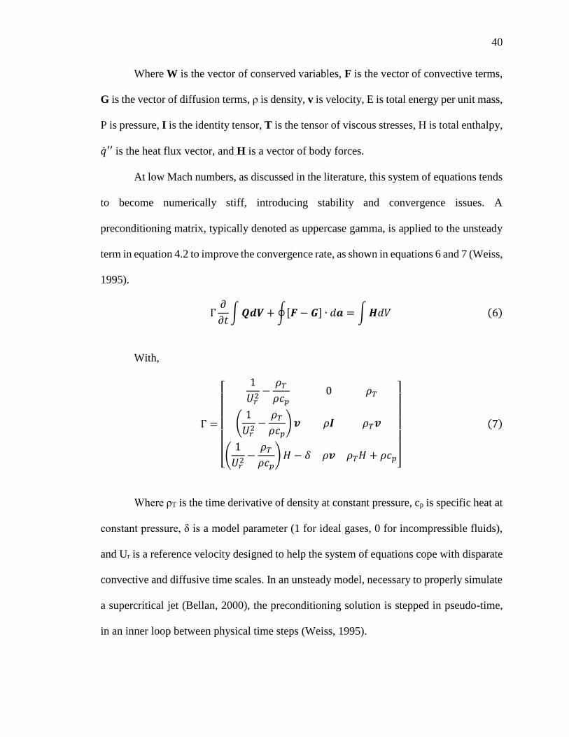
40
Where W is the vector of conserved variables, F is the vector of convective terms,
G is the vector of diffusion terms, ρ is density, v is velocity, E is total energy per unit mass,
P is pressure, I is the identity tensor, T is the tensor of viscous stresses, H is total enthalpy,
��′′ is the heat flux vector, and H is a vector of body forces.
At low Mach numbers, as discussed in the literature, this system of equations tends
to become numerically stiff, introducing stability and convergence issues. A
preconditioning matrix, typically denoted as uppercase gamma, is applied to the unsteady
term in equation 4.2 to improve the convergence rate, as shown in equations 6 and 7 (Weiss,
1995).
Γ𝜕
𝜕𝑡∫𝑸𝒅𝑽 + ∮[𝑭 − 𝑮] ∙ 𝑑𝒂 = ∫𝑯𝑑𝑉 (6)
With,
Γ =
[
1
𝑈𝑟2−
𝜌𝑇
𝜌𝑐𝑝0 𝜌𝑇
(1
𝑈𝑟2−
𝜌𝑇
𝜌𝑐𝑝)𝒗 𝜌𝑰 𝜌𝑇𝒗
(1
𝑈𝑟2−
𝜌𝑇
𝜌𝑐𝑝)𝐻 − 𝛿 𝜌𝒗 𝜌𝑇𝐻 + 𝜌𝑐𝑝
]
(7)
Where ρT is the time derivative of density at constant pressure, cp is specific heat at
constant pressure, δ is a model parameter (1 for ideal gases, 0 for incompressible fluids),
and Ur is a reference velocity designed to help the system of equations cope with disparate
convective and diffusive time scales. In an unsteady model, necessary to properly simulate
a supercritical jet (Bellan, 2000), the preconditioning solution is stepped in pseudo-time,
in an inner loop between physical time steps (Weiss, 1995).

41
Reynolds-Averaged Navier-Stokes
The full Navier-Stokes equations are not solved numerically in STAR-CCM+.
Instead, they are subjected to a Reynolds decomposition, resulting in the Reynolds-
Averaged Navier Stokes (RANS) equations. The Reynolds decomposition consists of
breaking a solution variable into parts, as shown in equation 8.
𝜙 = �� + 𝜙′ (8)
Where 𝜙 is a primitive variable such as pressure, or a velocity component, �� is an
averaged value, and 𝜙′ is its fluctuating component. For a steady solution, this averaging
is analogous to time-averaging, and for unsteady solutions, it is an average of inner
iterations. The mean-value momentum conservation equation now contains an extra term,
as shown in equations 9 and 10.
𝜕
𝜕𝑡(𝜌��) + ∇ ∙ (𝜌��×��) = −𝛁 ∙ ��𝑰 + ∇ ∙ (𝑻 + 𝑻𝒕) + 𝒇𝒃 (9)
Where Tt is the Reynolds stress tensor,
𝑻𝒕 = −𝜌 [𝑢′𝑢′ 𝑢′𝑣′ 𝑢′𝑤′
𝑢′𝑣′ 𝑣′𝑣′ 𝑣′𝑤′
𝑢′𝑤′ 𝑣′𝑤′ 𝑤′𝑤′ ] (10)
Closure to the RANS equations is achieved by modeling this tensor in terms of the
averaged value of primitive variables (Reynolds, 1895). This is most commonly performed
by an eddy-viscosity model.
k-Omega SST Turbulence Model
All eddy viscosity turbulence models are based on the Boussinesq hypothesis,
which states that the momentum transfer associated with turbulent eddies can be

42
approximated with an eddy viscosity term, μt (Boussinesq, 1877). Equation 11 shows how
the Reynolds stress tensor can now be made proportional to the mean strain rate tensor.
𝑻𝒕 = 2𝜇𝑡𝑺 −2
3(𝜇𝑡𝛁 ∙ ��)𝑰 (11)
This relationship assumes isotropy in turbulence, and for most flows and ideal gases
this does not present a significant problem. However, in near- and supercritical media,
where flow variables, thermodynamic properties and transport properties can all have large
spatial and temporal gradients, the Boussinesq assumption is probably not appropriate.
Additionally, the fluctuating component of the Reynolds decomposition described above
assumes constant fluid properties. These effects can effectively “smear-out” real-fluid
phenomena during model run-time and currently represent a fundamental limitation to
RANS models with respect to SC fluids.
k-omega SST is a two-equation turbulence model noted for its superior
performance in calculating boundary layers with adverse pressure gradients, jets and shear
flows, and its versatility in simultaneously handling wall-bounded flows and the freestream
without modification (Menter, 1994). It is less sensitive to inlet boundary conditions than
the also widely-used k-epsilon two-equation model. It uses two new transport properties, a
turbulent kinetic energy term, k, and a specific turbulent dissipation rate, ω. SST is
presented in equations 12 and 13.
𝜕
𝜕𝑡(𝜌𝑘) + ∇ ∙ (𝜌𝑘��) = 𝛁 ∙ [(𝜇 + 𝜎𝑘𝜇𝑡)∇𝑘] + 𝑃𝑘 − 𝜌𝛽∗𝑓𝑏∗(𝜔𝑘 − 𝜔0𝑘0) (12)
𝜕
𝜕𝑡(𝜌𝜔) + ∇ ∙ (𝜌𝜔��) = ∇ ∙ [(𝜇 + 𝜎𝜔𝜇𝑡)∇𝜔] + 𝑃𝜔 − 𝜌𝛽𝑓𝛽(𝜔2 − 𝜔0
2) (13)
Where 𝜎𝑘 and 𝜎𝜔 are model coefficients, Pk and Pw are production terms, 𝑓𝑏∗ is the

43
free-shear modification factor, and 𝑓𝛽 is the vortex stretching modification factor.
Large Eddy Simulation
STAR-CCM+ also features an LES solver. Large eddy simulation is seen as a
compromise between the computationally expedient but lower-fidelity RANS and
computationally prohibitive but highly realistic Direct Numerical Simulation (DNS)
approaches to modeling. A decomposition of flow variables still takes place, but instead of
Reynolds averaging, the variables are split spatially according to the size of the
computational grid, as shown in equation 14.
𝜙 = �� + 𝜙′ (14)
Where the tilde overbar represents the filtered value, and the prime represents the
sub-grid value. The filtered values are used in governing equations of the same form seen
above in the RANS model. The added turbulent stress tensor term Tt,, however, now
represents stresses on the subgrid scale, as shown in equation 15.
𝑻𝒕 = 2𝜇𝑡𝑺 −2
3(𝜇𝑡∇ ∙ �� + 𝜌𝑘)𝑰 (15)
Where �� is the large-scale filtered velocity and k is SGS turbulent kinetic energy.
This still constitutes a Boussinesq assumption, but on a much smaller scale than with
turbulence closure methods used with Reynolds averaging. With LES, flow is fully
resolved (no turbulence model required) on scales larger than the grid size, and a sub-grid
scale (SGS) model achieves turbulence closure on the smallest scales. STAR-CCM+ offers
three choices of SGS model. The default model, Wall-Adapting Local-Eddy Viscosity
(WALE) is similar to the older Smagorinsky SGS model, with the advantages of less

44
sensitivity to model coefficient choices no requirement of near-wall damping, similar to
Menter’s SST contribution to the k-omega model (Nicoud, 1999).
NIST REFPROP Data
Thermodynamic and transport properties of nitrogen were extracted from
REFPROP, a software package released by NIST, using an open-source MATLAB script
and compiled into .csv files. These files contain pressure-temperature tabulated fluid
properties and partial derivatives, and were imported into each STAR-CCM+ simulation
file. The code linearly interpolates these tables at each iteration, assigning a realistic fluid
property for each thermodynamic state. Properties were sampled from the library from 64
K to 1000 K and from 0 MPa to 5 MPa, at 500 temperature levels and 500 pressure levels.
Speed of sound, specific heats, enthalpy, thermal conductivity, dynamic viscosity, density
and entropy were included in the model.
Boundary and Initial Conditions
The 2D computational domain has five boundaries: two walls bounding the flow in
the transverse direction, an outlet, a wall bounding the inlet, and the inlet itself. A pressure
outlet set to ambient pressure was selected at the outlet boundary, as this is the
recommended boundary type for this flow regime and solver type, and is typical of the
literature. No additional settings were changed at the outlet. No-slip, adiabatic walls were
selected for all three wall locations. No additional settings were changed for the wall
boundaries.
The experiment specified an operating pressure, inlet temperature and injected jet
velocity, so a velocity inlet was selected to the injector boundary. For the first several

45
simulations, only injection velocity and temperature were changed on the inlet. All other
properties and values were left at default. Attempting to better match results, inlet
conditions were adjusted to represent the fully-developed turbulent pipe flow at jet exit
described in the experiment (Bellan, 2002). Velocity inlet settings are shown in Table 3.4.
Table 3.4 Inlet Boundary Condition Parameters
Initial Runs Matching Experiment
Static Temperature 126.9 K 126.9 K
Turbulence Intensity 0.01 0.0356
Turbulent Length Scale 0.01 m 8.36 E-5 m
Velocity Magnitude 5.04 m/s (constant) Nikuradse Profile, Mean Velocity 5.04 m/s
Turbulence intensity and length scale were calculated based on mean flow velocity
and injector diameter according to equations 16 and 17 (Siemens PLM).
𝐼 = 0.16𝑅𝑒−18 (16)
𝐿0 = 0.038𝐷ℎ (17)
Where Dh is the hydraulic diameter of the channel.
The Nikuradse velocity profile, shown in equation 18, is a relatively flat function
of pipe radius (y-distance) representative of fully-developed turbulent flow (Tuoc, 2009).
𝑢
��= (
𝑦
𝑅)
1𝑛
(18)
Where �� is a time averaged velocity at pipe centerline, R is pipe radius, and n is a
parameter depending on Reynolds number. Here, n =7 for Re ≈ 105.
The 3D quarter-jet boundary conditions are similar, with the inclusion of periodic
interfaces on the bottom and left symmetry planes (matching the flow solution on these
surfaces) and modeling the inlet velocity profile as a function of radius rather than height.

46
First cases were run with an initially flat solution space at chamber temperature and
pressure. The STAR-CCM+ Coupled Solver’s Expert Initialization feature was used to
produce an approximate inviscid flow solution. This feature initializes the pressure,
velocity and temperature fields and reduces overall computation time.
Model settings: RANS
Physics models included in RANS simulations are presented in Table 3.5.
Table 3.5 Physics Models Used in RANS Simulation
Implicit Unsteady User Defined EOS* Two Dimensional
All y + Wall Treatment SST (Menter) K-Omega K-Omega Turbulence
Reynolds-Averaged Navier- Stokes
Coupled Energy Exact Wall Distance
Turbulent Gradients Coupled Flow
Gas
* A number of initial runs were made using the Ideal Gas and Peng-Robinson Real
Gas equations of state but this configuration represents the bulk of results presented below.
Most of the models described in the literature use very high order solvers. In STAR-
CCM+ RANS, the highest available solvers were selected: 2nd-order implicit in space and
2nd order implicit in time. The Expert Driver feature was enabled in the Coupled Solver to
help balance stability and convergence rate. It includes an algorithm to automatically
throttle the Courant-Friedrichs-Lewy (CFL) number. Reasonable residual convergence
was achieved using a time step of 5E-6 s and 10 iterations per time step.
Model Settings: LES
Physics models included in LES cases are presented in table 4.6.

47
Table 3.6 Physics Models Included in LES Simulation
Coupled Energy All y + Wall Treatment Exact Wall Distance
WALE Subgrid Scale Large Eddy Simulation Turbulent
User Defined EOS Gradients Coupled Flow
Gas Implicit Unsteady Three Dimensional
Using LES in STAR-CCM+ gives the user access to higher order solvers. The
MUSCL 3rd-order/CD solver was selected in space and 2nd-order implicit solver selected
in time. The MUSCL solver is intended for highly-accurate simulations of aeroacoustics
and aerodynamics and has a built in gradient threshold trigger that switches to a lower-
order solver to maintain stability. Nominally it is a blended 3rd-order upwind/3rd-order
centered-difference solver, and switches to a 1st-order ENO solver when high gradients are
encountered. Time stepping was not refined for this model to the extent of the RANS case,
as the computation time LES demands required focus to be returned to RANS simulation.
Time step here was 3E-4 s, with 15 iterations per time step. A coarse time step is a likely
source of error in LES results.
Original Test Case Matrix
Table 3.7 outlines the original benchmarking test matrix
Table 3.7 Benchmarking Test Matrix
RANS Subcritical Jet, Ideal Gas EoS
SC Jet, PR EoS SC Jet, REFPROP data
LES Control case Tune Inlet Conditions
Grid/Time Step Independence
The LES model was initially found more sensitive to inlet conditions than the
RANS model, and an incremental approach to benchmarking was desired. As the original
intent was an applied study of mixing for injector design, this was to be followed by an

48
aggressive campaign of simultaneous RANS simulations on local computing assets and
LES simulations on a parallel cluster. Results would then be compared to evaluate the
fidelity of the less computationally-expensive method. Table 3.8 outlines the intended path.
Table 3.8 Nominal Test Matrix
RANS LES
Introduce Crossflow to Single Jet Introduce Crossflow to Single Jet
Introduce Coaxial Shell Flow (Oxidizer), Quiescent Chamber
Introduce Coaxial Shell Flow (Oxidizer), Quiescent Chamber
Multispecies Coaxial Flow Multispecies Coaxial Flow
Multispecies Co-Axial Flow into Crossflow Multispecies Co-Axial Flow into Crossflow
Combustion Case, Tabular Combustion Method
Combustion Case, Tabular Combustion Method
Challenges with LES and Lessons Learned
Simply stated, a gross underestimation was made of the processor-hours required
to perform a thorough LES treatment of a domain of this size. Flow times on the order of
0.1 s take approximately 24 hours using 72 processors with the current grid, and a large
number of runs are necessary to tune and debug a LES simulation. Achieving a benchmark
and generating a new grid with more complicated flow and geometry (and wall effects)
and troubleshooting the new grid in the required time was, in hindsight, unrealistic. The
work necessary for an unsteady combustion simulation campaign in a poorly-understood
thermodynamic regime is also likely beyond the scope of a Master’s thesis. There remains,
however, much to be learned from results that were obtained.
Revised Test Case Matrix
Qualitative LES results were achieved for one case, but mesh independence was

49
not established, and there are notable differences to previous work. Effort was refocused
on 2D RANS modeling to ensure that some meaningful results were obtained in the time
permitted, and to enable some qualitative conclusions to be drawn. The final test matrices
are presented in Table 3.9, Table 3.10, and Table 3.11.
Table 3.9 Test Case Matrix: Supercritical Jet
Supercritical Jet – User-Defined EoS
Steady Unsteady
1st-Order Solvers 2nd-Order Solvers
1st-Order Solvers 2nd-Order Solvers
Reference Mesh Reference Mesh Reference Mesh Reference Mesh
Mesh Level 2 Mesh Level 2 Mesh Level 2 Mesh Level 2
Mesh Level 3 Mesh Level 3 Mesh Level 3 Mesh Level 3
Table 3.10 Test Case Matrix: Atmospheric Jet, User-Defined EoS
Atmospheric Jet – User-Defined EoS
Steady Unsteady
1st-Order Solvers 2nd-Order Solvers
1st-Order Solvers 2nd-Order Solvers
Reference Mesh Reference Mesh Reference Mesh Reference Mesh
Mesh Level 2 Mesh Level 2 Mesh Level 2 Mesh Level 2
Mesh Level 3 Mesh Level 3 Mesh Level 3 Mesh Level 3
Table 3.11 Test Case Matrix: Atmospheric Jet, Ideal Gas EoS
Atmospheric Jet – Ideal Gas EoS
Steady Unsteady
1st-Order Solvers 2nd-Order Solvers
1st-Order Solvers 2nd-Order Solvers
Reference Mesh Reference Mesh Reference Mesh Reference Mesh
Mesh Level 2 Mesh Level 2 Mesh Level 2 Mesh Level 2
Mesh Level 3 Mesh Level 3 Mesh Level 3 Mesh Level 3
Grid Independence
Grid independence was evaluated by comparing density and axial velocity plots

50
along the jet centerline and axial velocity profiles at several streamwise locations.
Comparisons are made using time-averaged data on unsteady solutions. Independence is
established at mesh level 2. The Reynolds number independence was not considered, as
SC jet mixing behavior is seen in the literature to depend chiefly on the thermodynamic
state of the injected fluid rather than injection speed (Zong, 2004). Centerline density for
all three grid levels is presented in Figure 3.2.
Figure 3.2 Centerline Density: Unsteady RANS
Three important features are very similar between these three plots. Core
penetration is approximately 8-10 jet diameters for all cases. Centerline density appears to
approach 150 kg/m3 at 30 jet diameters in all cases. The slope of density decay in the
transition zone matches closely between grid levels 2 and 3, and grid independence is
declared for mesh level 2 for this criterion. Centerline axial velocity is compared in Figure
3.3.
0
50
100
150
200
250
300
350
400
450
500
0 5 10 15 20 25 30
Den
sity
[kg
/m3]
x/D
Reference Mesh
Mesh Level 2
Mesh Level 3
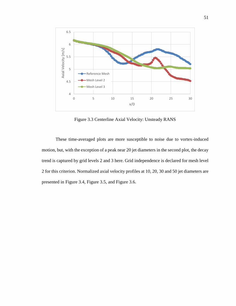
51
Figure 3.3 Centerline Axial Velocity: Unsteady RANS
These time-averaged plots are more susceptible to noise due to vortex-induced
motion, but, with the exception of a peak near 20 jet diameters in the second plot, the decay
trend is captured by grid levels 2 and 3 here. Grid independence is declared for mesh level
2 for this criterion. Normalized axial velocity profiles at 10, 20, 30 and 50 jet diameters are
presented in Figure 3.4, Figure 3.5, and Figure 3.6.
4
4.5
5
5.5
6
6.5
0 5 10 15 20 25 30
Axi
al V
elo
city
[m
/s]
x/D
Reference Mesh
Mesh Level 2
Mesh Level 3

52
Figure 3.4 Axial Velocity Profiles: Unsteady RANS, Reference Mesh
Figure 3.5 Axial Velocity Profiles: Unsteady RANS, Mesh Level 2
-0.2
0
0.2
0.4
0.6
0.8
1
1.2
-12 -8 -4 0 4 8 12
u/u
_0
r/D
x/D = 10
x/D = 20
x/D = 30
x/D = 50
0
0.1
0.2
0.3
0.4
0.5
0.6
0.7
0.8
0.9
1
-15 -10 -5 0 5 10 15
u/u
_0
r/D
x/D = 10
x/D = 20
x/D = 30
x/D = 50

53
Figure 3.6 Axial Velocity Profiles: Unsteady RANS, Mesh Level 3
With the exception of the axial velocity distribution at 50 jet diameters, this data
matches quite well in all three cases. Grid independence from this perspective is achieved
at the reference grid level. Overall, grid independence is declared at grid level 2, and that
data is used for unsteady RANS results in the following section.
-0.1
0
0.1
0.2
0.3
0.4
0.5
0.6
0.7
0.8
0.9
1
-12 -8 -4 0 4 8 12
u/u
_0
r/D
x/D = 10
x/D = 20
x/D = 30
x/D = 50

54
4. Results and Discussion
The following chapter presents and discusses data gathered from several RANS
simulations and one LES simulation of a test case from a 2002 Branam and Mayer
experiment (Branam, 2002). Current data is compared to the original experimental data as
well as results from an LES simulation conducted by Hickey and Ihme using Stanford’s
CharLESx solver. First is a walkthrough of initial incremental RANS benchmarking efforts.
This is followed by the author’s attempt to harness the power and accuracy of LES, and
finally an extensive comparison of RANS results using NIST REFPROP data.
Preliminaries: First Steps in Benchmarking
An incremental approach to modeling supercritical fluids was taken to ensure the
best possible matching of previous results. Elements of added complexity were added one
at a time, beginning with a subcritical case using software default settings. If the reader
prefers to proceed directly to results, they are discussed for unsteady RANS and LES using
real fluid properties and inlet conditions are presented in the next section.
An atmospheric jet using the ideal gas EoS is first simulated for illustrative
purposes, and for comparison to supercritical cases using the same code. Several initial
steady-state runs were based on half-jet grids with a symmetry plane along the jet
centerline. This grid is equivalent to the top half of the reference grid described in the
previous section and an example is shown in Figure 4.1.

55
Figure 4.1 Half-jet velocity contour, reference mesh
Density is plotted along the jet centerline for a subcritical jet in Figure 4.2.
Figure 4.2 Centerline Density of a 1 atm jet using ideal gas EoS
This illustrates typical single-phase gas jet behavior. A relatively intact potential
core is seen penetrating to approximately 12 jet diameters, a transition region follows as
jet density decays between 12 and 25 jet diameters, and self-similarity is achieved in the
vicinity of 30-40 jet diameters. The half-jet grid is used because of a jet curving tendency
tentatively attributed to baroclinic torque, as discussed in (Zong, 2004). This is examined
in Figure 4.3 and Figure 4.4.
0
0.5
1
1.5
2
2.5
3
0 5 10 15 20 25 30
Den
sity
[kg
/m3 ]
x/D

56
Figure 4.3 Pressure contour of a steady-state jet
Figure 4.4 Density contour of a steady-state jet
This causes curvature in the jet, complicating analysis of velocity profiles and
properties along the centerline. For this reason, all data for steady jets is taken from half-
jet grids. This does not significantly impact results, as the flow physics of the jets of interest
is inherently unsteady, and is analyzed as such (Bellan, 2000).
It is obvious that the ideal gas EoS is not suitable for a simulation at supercritical
temperature and pressure. At 4 MPa and 298 K, the chamber conditions of Bellan’s 2002
experiment, the ideal gas law under-predicts density by approximately 50%. The Peng-
Robinson real gas EoS is substituted into the model. A brief error analysis is performed to
ascertain its accuracy relative to the ideal gas EoS, as shown in Figure 4.5, Figure 4.6,
Figure 4.7 and Figure 4.9.

57
Figure 4.5 N2 Density Calculation Using PR EoS Compared to NIST Data on a 3.5 MPa
Isobar
Figure 4.6 N2 Density Calculation Using PR EoS Compared to NIST Data on a 130 K
Isotherm
0
100
200
300
400
500
600
700
110 120 130 140 150 160
Den
sity
[kg
/m^3
]
T [K]
STAR-CCM+
EoS Solution
NIST Data
0
50
100
150
200
250
3 3.1 3.2 3.3 3.4 3.5 3.6 3.7
Den
sity
[kg
/m^3
]
P [MPa]
STAR-CCM+
EoS Solution
NIST Data

58
Figure 4.7 Percent Error of Density Calculation on an Isobar
Figure 4.8 Percent Error of Density Calculation on an Isotherm
This compares well with the EoS errors cited in the literature for density
calculations, and errors of approximately 5% are generally considered acceptable in this
region. A centerline density plot for a STAR-CCM+ steady supercritical jet, using the PR
EoS, is shown in Figure 4.9.
0
1
2
3
4
5
6
110 115 120 125 130 135 140 145 150 155
Erro
r [%
]
T [K]
STAR-CCM+ Error %
EoS Solution Error %
4.5
4.6
4.7
4.8
4.9
5
5.1
5.2
3 3.1 3.2 3.3 3.4 3.5 3.6 3.7
Erro
r [%
]
P [MPa]
STAR-CCM+ Error %
EoS Solution Error %

59
Figure 4.9 Centerline Density of a supercritical jet using the PR EoS, constant properties
The proper density ranges at experiment operating conditions are now represented.
The density profile is compared to published CharLES results from Hickey and Ihme,
matching experimental data from Branam and Mayer’s much cited 2002 experiment
(Hickey, 2013) in Figure 4.10.
0
50
100
150
200
250
300
350
400
450
500
0 5 10 15 20 25 30 35
Den
sity
[kg
/m3 ]
x/D

60
Figure 4.10 Centerline Density Comparison to CharLES results
The current model captures centerline density decay, but does not contain the
characteristic sharp inflection at the end of the potential core and overpredicts the core
penetration. To this point, simulations have been run assuming constant fluid properties,
including viscosity, specific heat, and thermal conductivity. The literature makes it quite
clear that this is an unrealistic assumption, given the degree to which fluid properties vary
in this thermodynamic regime. Going forward, a user-defined EoS is used, consisting of
complete nitrogen property data stored in pressure-temperature lookup tables which are
extracted from the NIST code REFPROP, and imported into the STAR-CCM+ simulation
files. Figure 4.11 shows the effect of this change on the density profile.
0
50
100
150
200
250
300
350
400
450
500
0 5 10 15 20 25 30 35
Den
sity
[kg
/m3 ]
x/D
STAR-CCM+Results, PR EoS
CharLES Results(Hickey, 2013)

61
Figure 4.11 Centerline Density Comparison to CharLES Results, User-Defined EoS
Potential core penetration is significantly reduced, and self-similar region density
approaches previous results. This is good evidence that use of real fluid properties adds
fidelity to the simulation. The LES case is presented next in some detail.
LES Results
Large eddy simulation was run for 680 ms of flowtime (sufficient for more than 3
flow-throughs) in a symmetrical quarter jet, in a grid of approximately 11.5 million control
volumes. Jet exit velocity profile, turbulence intensity and turbulent length scales are
configured to represent fully developed turbulent pipe flow. Axial velocity profile giving
a mean flow velocity of 5.04 m/s at jet exit is presented in Figure 4.12.
0
50
100
150
200
250
300
350
400
450
500
0 5 10 15 20 25 30 35
Den
sity
[kg
/m3]
x/D
STAR-CCM+, UD EoS
CharLES Results(Hickey, 2013)

62
Figure 4.12 Nikurasde Fully Developed Turbulent Flow Velocity Profile
Figure 4.13, Figure 4.14, Figure 4.15 and Figure 4.16 compare velocity magnitude
and temperature contours to CharLES results from (Hickey, 2013). CharLES contours are
white-hot, with velocity range of 0-5.6 m/s, and temperature range of 125.6 to 306.7 K.
Figure 4.13 Velocity Magnitude Contour, CharLES Results (Hickey, 2013)
Figure 4.14 Velocity Magnitude Contour, LES Results, Current Work
0
1
2
3
4
5
6
7
0 0.0005 0.001 0.0015 0.002
Axi
al v
elo
city
[m
/s]
Inlet Position [m]

63
Figure 4.15 Temperature Contour, CharLES Results, (Hickey, 2013)
Figure 4.16 Temperature Contour, LES Results, Current Work
These snapshot contours indicate that similar flow feature scales are being captured
in both simulations, but diffusion of jet velocity and temperature is slower in current work.
Jet centerline density for the current simulation is shown in Figure 4.17.
Figure 4.17 Centerline Density, LES Results, 680 ms Flowtime, Current Work
The trend of decay is captured, but potential core penetration again does not exactly
0
50
100
150
200
250
300
350
400
450
500
0 5 10 15 20 25 30
Den
sity
[kg
/m3 ]
x/D
LES Results, CurrentWork
CharLES Results(Hickey, 2013)

64
match previous results. The penetration length is however closer to previous work, but
STAR-CCM+ LES here under-predicts the penetration by approximately 2 jet diameters.
RANS Results: Comparison with Previous Work
Velocity magnitude and temperature (snapshot) contours are compared to CharLES
results in Figure 4.18, Figure 4.19, Figure 4.20, and Figure 4.21.
Figure 4.18 Velocity Magnitude Contour, CharLES Results, (Hickey, 2013)
Figure 4.19 Velocity Magnitude Contour, RANS Results, Current Work

65
Figure 4.20 Temperature Contour, CharLES Results, (Hickey 2013)
Figure 4.21 Temperature Contour, RANS Results, Current Work
Again, velocity magnitude and temperature are diffused much more quickly in
CharLES results, and flow feature scale is coarser in this RANS simulation. Centerline
density decay is better predicted compared with CharLES, however, as shown in Figure
Figure 4.22.

66
Figure 4.22 RANS Centerline Density Compared to CharLES Results
This is the best density decay agreement seen so far, although a slight
overprediction of potential core penetration persists. Figure 4.23 shows centerline density
experimental data and RANS model results for a similar but not identical case from
(Branam, 2003), normalized with respect to density at jet exit. It is compared to current
results.
0
50
100
150
200
250
300
350
400
450
500
0 5 10 15 20 25 30 35
Den
sity
[kg
/m3 ]
x/D
Unsteady RANS, CurrentWork
CharLES Results (Hickey,2013)

67
Figure 4.23 Centerline Density: Current Work Compared to Case 6 (3.9 MPa, 133 K, 5.4
m/s), (Branam, 2003)
Branam and Mayer find this is a short core penetration relative to their entire test
matrix. They suggest this may be due to the heat transfer phenomenon characteristic to
supercritical fluid; this case in particular features a jet injected above the temperature range
for enhancement, and the jet needs to absorb less energy to achieve ambient temperature.
The jet thus dissipates more smoothly, resulting in a shorter core. This case in particular
speaks well of current modeling efforts, as the jet with which current work is compared is
injected at a higher temperature, its temperature reaches the ambient condition more
quickly, and density decays faster (6-7 jet diameters vs. the current 8-9). Core penetration
is compared with overall experimental results in (Branam, 2003) as they plot this
characteristic with respect to ratio of injected jet density to ambient density in Figure 4.24.
Calculated density ratio of current work is approximately 10.07.
0
0.2
0.4
0.6
0.8
1
1.2
0 5 10 15 20 25 30
ρ/ρ
_max
x/D
Unsteady RANS, CurrentWork
Model (Branam, 2003)
Experiment (Branam,2003)

68
Figure 4.24 Potential Core Penetration vs. Density Ratio (Branam, 2003)
Current unsteady RANS results, suggesting a penetration of 8-9 jet diameters
(indicated by the red arrow), agree well with the majority of data represented on this plot
for an injected/ambient density ratio of 10. Current RANS results indicate an under-
prediction of penetration, about 4 jet diameters, indicated by the blue arrow.
Axial velocity profiles normalized with respect to individual profile maximum
velocities are presented in Figure 4.25.

69
Figure 4.25 Axial Velcocity Profiles, Unsteady RANS
Resulting jet half-width locations are presented in Figure 5.25.
Figure 4.26 Jet Half-Width Locations, Unsteady RANS
The half-angle of jet divergence is calculated as ∝= 𝑡𝑎𝑛−1 (𝑟/𝐷
𝑥/𝐷) using axial
velocity data for the first 30 jet diameters. The spreading angle (twice the half-angle) from
current work is approximately 10.94°. This is compared to tabulated data from (Branam,
0
0.1
0.2
0.3
0.4
0.5
0.6
0.7
0.8
0.9
1
-15 -10 -5 0 5 10 15
u/u
_0
r/D
x/D = 10
x/D = 20
x/D = 30
x/D = 50
-10
-8
-6
-4
-2
0
2
4
6
8
10
0 10 20 30 40 50 60
r/D
x/D

70
2003) in Figure 4.27.
Figure 4.27 Tabular Jet Spreading Angle Data (Branam, 2003)
Case 5, to which we compare, shows a slightly lower density ratio, and a smaller
calculated spreading angle with respect to axial velocity. The calculated angle from current
work however falls evenly between Raman and shadowgraph technique measurements.
A density contour from current work is compared against a shadowgraph image
from (Branam, 2002) for a similar case injected jet in Figure 4.28, and Figure 4.29.

71
Figure 4.28 Shadowgraph Image: Case 3, 4 MPa, 4.9 m/s, 123 K Injected N2 Jet
(Branam, 2002)
Figure 4.29 Density Contour (Snapshot) Unsteady RANS, Current Work
The current model shows a greater propensity for the jet to cast off large eddies
asymmetrically, and does not capture the small, sub-millimeter scale density fluctuations
of the experiment. This shadowgraph image, however, captures approximately only the
first 13 jet diameters, and would be mostly composed of potential core. All contours

72
representing current work capture up to 30 jet diameters. A shadowgraph of the same flow
case from Branam & Mayer’s 2002 paper is presented overlaid with contours
corresponding to measured streamwise turbulent length scales in Figure 4.30 and
transverse length scales in Figure 4.31.
Figure 4.30 Streamwise Direction Turbulent Length Scales, Case 3 (Branam, 2002)
Figure 4.31 Transverse Direction Turbulent Length Scales, Case 3 (Branam, 2002)

73
The length scales observed in this 2002 experiment, as seen below, match well with
calculated Taylor microscales, which are generally within one order of magnitude of jet
exit diameter in this case. Turbulent length scales for current work are estimated based on
model transport quantities. Integral, Taylor and Kolmogorov microscales are calculated
according to equations 1-4, per (Branam, 2002).
𝐿𝑖𝑛𝑡 =𝑘
32
휀(1)
𝐿𝑇𝑎𝑦 = (15𝜈��2
휀)
12
(2)
Where,
�� = (𝑢2 + 𝑣2 + 𝑤3
3)
12
(3)
𝐿𝐾𝑜𝑙 = (𝜈3
휀)
14
(4)
Using a k-omega model, the definition of specific turbulent dissipation is used and
shown in equations 5 and 6:
𝜔 =휀
𝑘𝛽∗(5)
휀 = 𝜔𝑘𝛽∗ (6)
Where k is turbulent kinetic energy, ε is turbulent dissipation rate, ν is kinematic
viscosity, u and v are velocities, ω is specific turbulence dissipation, and β* is a k-omega
turbulence model constant, usually 0.09, which is used in this case.
Estimated integral length scales are presented in Figure 4.32, Taylor microscales
are presented in Figure 4.33, and Kolmogorov microscales are presented in Figure 4.34.

74
Figure 4.32 Integral Length Scales at Various x/D Locations, Unsteady RANS
Figure 4.33 Taylor Microscales at Various x/D Locations, Unsteady RANS
1.00E-04
1.00E-03
1.00E-02
-8 -6 -4 -2 0 2 4 6 8
Len
gth
sca
le [
m]
r/D
x/D = 10
x/D = 20
x/D = 30
1.00E-05
1.00E-04
1.00E-03
1.00E-02
1.00E-01
-8 -6 -4 -2 0 2 4 6 8
Len
gth
sca
le [
m]
r/D
x/D = 10
x/D = 20
x/D = 30

75
Figure 4.34 Kolmogorov Microscales at Various x/D Locations, Unsteady RANS
Length scales are compared to those calculated for Branam’s 2003 experiment,
normalized with respect to jet diameter. Calculated length scales are compared in Figure
4.35.
Figure 4.35 Calculated Turbulent Length Scales
1.00E-06
1.00E-05
1.00E-04
-8 -6 -4 -2 0 2 4 6 8
Len
gth
sca
le [
m]
r/D
x/D = 10
x/D = 20
x/D = 30
0.0001
0.001
0.01
0.1
1
10
100
0 0.5 1 1.5 2 2.5 3 3.5 4 4.5 5
L/D
r/D
Integral: Current Work Taylor: Current Work
Kolmogorov: Current Work Integral (Branam, 2003)
Taylor (Branam 2003) Kolmogorov (Branam, 2003)

76
There is a difference in magnitude between calculated values at this location
between the two simulations, as the relative size of integral and Taylor microscales seem
to reverse in current work. This can partially be attributed to Branam’s use of a different
commercial code with k-epsilon closure vs the current use of a k-omega closure. This also
highlights the need for tuning of the turbulence model parameters of current work.
Although the magnitude of these length scales differ, the trend is the same, and the
Kolmogorov scale matches well. Other properties and settings of Branam’s code are
unknown at this time.
RANS Results: Comparison of Subcritical and Supercritical Results
Results from unsteady RANS modeling of a supercritical jet are here compared
with single-phase gas jet mixing simulations run at subcritical pressures to demonstrate the
ability of the current code to represent key differences (and similarities) in flow physics,
and to highlight the importance of modeling real gas effects in the supercritical regime.
Centerline density profiles are shown in figure Figure 4.36, normalized with respect to jet
exit density.

77
Figure 4.36 Normalized Centerline Density: Supercritical and two Subcritical
Simulations, Unsteady RANS, Current Work
This figure serves to illustrate the effect of modeling real gas effects even at
atmospheric conditions, as the subcritical case described above was run with ambient
conditions of 298 K and 1 atm. The supercritical case has a shorter core penetration, and
the density decay in the transition region is more aggressive, given the much stronger
density gradient. Centerline axial velocity decay is compared for these cases in Figure 4.37.
0
0.2
0.4
0.6
0.8
1
1.2
0 5 10 15 20 25 30
ρ/ρ
_max
x/D
Supercritical
Subcritical, User-Defined EoS
Subcritical, IdealGas EoS

78
Figure 4.37 Centerline Axial Velocity: Supercritical and two Subcritical Simulations,
Unsteady RANS, Current Work
Unsurprisingly, the supercritical case shows a slower decay of axial velocity at the
centerline, as fluid speed is matched but density and therefore kinetic energy of the jet is
much higher in that case. Interestingly, using real fluid properties has a large impact on the
dissipation of energy from the jet, and this is likely due to variation in dynamic viscosity
in the transverse direction, as this is transport quantity is what will regulate the exchange
of momentum across the shear layer of the jet. This difference is examined in Figure 4.38.
2
2.5
3
3.5
4
4.5
5
5.5
6
6.5
0 5 10 15 20 25 30
Axi
al V
elo
city
[m
/s]
x/D
Supercritical
Subcritical, User-Defined EoS
Subcritical, IdealGas EoS

79
Figure 4.38 Dynamic Viscosity Profiles at x/D = 10: Supercritical and two Subcritical
Simulations, Unsteady RANS, Current Work
This confirms the above assumption, with supercritical case viscosity being several
times that of the real gas subcritical case. The assumption of constant fluid properties in
the ideal gas case (specifically μ=1.79E-5 Pa-s here) explains the similarity in velocity
decay between this case and the supercritical case in Figure 4.37. Note in particular how
the dynamic viscosity varies across the jet in the supercritical case (more than a factor of
two) and the sharpness of the viscosity gradient in the transverse direction. There are
similarly large gradients in specific heat, thermal conductivity and isentropic
compressibility in the shear layer.
Final Thoughts
The STAR-CCM+ RANS simulations described above capture the expected single-
phase gas jet mixing behavior expected in the literature. A strong tendency for asymmetric
vortex shedding is observed, indicating why unsteady simulation is preferred. Additionally,
7.50E-06
1.25E-05
1.75E-05
2.25E-05
2.75E-05
-4 -3 -2 -1 0 1 2 3 4
Dyn
amic
Vis
cosi
ty [
Pa
s]
r/D
Supercritical
Subcritical, User-DefinedEoS
Subcritical, Ideal Gas EoS

80
no atomization or droplet formation is produced. In a qualitative manner, a commercial
code, when fed real gas properties, reproduces the proper flow physics. However, the
results presented above indicate that the margin for error in specific measurements is high,
and much further fine-tuning of the commercial code is required to match experimental
data and previous numerical results. Although the accurate reproduction of supercritical
mixing phenomena absolutely requires real fluid thermodynamic and transport properties,
there is a computational cost associated with this, and in particular with the use of tabular
data. Based on the work performed here on a parallel cluster, the use of tables introduces a
27.2% increase in CPU-hours compared with use of standard equations of state. It should
be noted the majority of simulations were performed on a single cluster node, and this
additional cost is not expected to scale linearly as cell counts grow and additional nodes
are added.
Plots of simulation residuals and important monitor quantities can be found in the
Appendix.

81
5. Conclusions and Recommendations
The commercial code STAR-CCM+ was demonstrated to reproduce the relevant
flow physics when using imported tabular real fluid data. The author remains confident
that a code such as this can be fine-tuned to more accurately represent mixing parameters
such as density decay, axial velocity profiles and species concentrations in a multi-species
flow. The code can then be applied to a cross-flow, and eventually inform a combustion
model. The goal of this work remains design-oriented, and will apply to injectors in direct-
fire s-CO2 power cycles and liquid-propellant rockets. The following observations were
made:
1. Of the model configurations examined, unsteady RANS simulation using k-
omega SST turbulence closure provided the closest match of core penetration
length to previous results. Still, there remains an over-prediction of potential
core penetration of approximately 30% (Hickey, 2013).
2. There is a strong tendency in current unsteady RANS simulation for the jet to
shed large vortices asymmetrically. This echoes previous assertions in the
literature that turbulent mixing of a supercritical jet is an inherently unsteady
phenomenon, and is why unsteady RANS simulation was necessary (Bellan,
2000).
3. Results from velocity magnitude and temperature contours of current unsteady
RANS show a slower velocity decay and slower transition to ambient
temperature than LES results in the literature (Hickey, 2013).
4. Small turbulent structures from LES in literature were not captured in current
unsteady RANS simulation, despite grid refinement. This is due to Reynolds

82
averaging of the flow and modeling of small turbulent eddies as eddy viscosity.
LES may be necessary to correctly predict penetration length, but further tuning
of the turbulence model parameters could reproduce previous work at less
computational expense. Current LES work needs model refinement but shows
flow features of similar scale to previous work.
Future Work
The constant properties assumption inherent to the Reynolds decomposition is a
necessary feature of all RANS simulation. This can, however, be mitigated by the future
development of turbulence models custom to the supercritical regime (Bellan, 2000).
Developing these models will likely require a certain amount of LES work, just as sub-grid
scale models for LES required research using DNS (Miller, 2001). Additional work is also
required in fine-tuning model and solver parameters to more closely capture the
experimental data.
Having determined the suitability for commercial code to tackle supercritical
mixing problems, important next steps toward the goals of improved injector design in
liquid rockets and s-CO2 cycles are:
1. Refine model constants and turbulent inlet conditions of unsteady RANS
simulation to better match Case 5 from (Branam, 2003).
2. Introduce a passive scalar into unsteady RANS simulations to better quantify
the mixing process. This is the numerical equivalent of injecting a dye into an
experiment, and will identify the path of injected fluid as the jet evolves.
3. Create 3D unsteady RANS domain (quarter-jet) for comparison to experiment.
4. Complete grid independence study in LES model, refine time step for better

83
residual convergence.
5. Refine model constants and turbulent inlet conditions of LES model to better
match Case 5 from (Branam, 2003) and CharLES results from (Hickey, 2013).
6. Compare unsteady RANS and LES results with the addition of a multispecies
crossflow.
7. Compare unsteady RANS and LES results with a multispecies crossflow and
co-axial injection of a fuel and oxidizer.

84
REFERENCES
About Us. Retrieved June 26, 2017 from http://www.cascadetechnologies.com/about-us/
Artham, S. K. (2016). An Experimental Study of Momentum-Driven Unsteady Jets.
Master of Science Thesis, Embry-Riddle Aeronautical University.
Barata, J., Gökalp, I., and Silva, A. (2003). Numerical Study of Cryogenic Jets Under
Supercritical Conditions. Journal of Propulsion and Power, 19(1), 142-147.
Bellan, J. (2000). Supercritical (and subcritical) fluid behavior and modeling: drops,
streams, shear and mixing layers, jets and sprays. Progress in Energy and
Combustion Science, 26, 329-366.
Benedict, M., Webb, G. B., and Rubin, L. C. (1940). An Empirical Equation for
Thermodynamic Properties of Light Hydrocarbons and Their Mixtures I.
Methane, Ethane, Propane and n-Butane. The Journal of Chemical Physics,
8(334).
Birk, A., McQuaid, M., and Gross, M. (1995). Liquid Core Structure of Evaporating
Sprays at High Pressures – Flash X-Ray Studies. Army Research Laboratory.
Boussinesq, J. (1877). Essai sur la théorie des eaux courantes. Paris, France : Imprimerie
Nationale.

85
Branam, R., and Mayer, W. (2002). Length scales in cryogenic injection at supercritical
pressure. Experiments in Fluids, 33, 422-428.
Branam, R., and Mayer, W. (2003). Characterization of Cryogenic Injection at
Supercritical Pressure. Journal of Propulsion and Power, 19(3), 342-355.
Brun, K., McClung, A., and Davis, J. (2014). Novel Supercritical Carbon Dioxide Power
Cycle Utilizing Pressurized Oxy-combustion in Conjunction with Cryogenic
Compression. Southwest Research Institute report.
Chehroudi, B., Talley, D., and Coy, E. (1999). Initial Growth Rate and Visual
Characteristics of a Round Jet into a Sub- to Supercritical Environment of
Relevance to Rocket, Gas Turbine, and Diesel Engines. 37th AIAA Aerospace
Sciences Meeting and Exhibit. 11-14 January, 1999, Reno, NV.
Chen, Y.-S., and Kim, S.-W. (1987) Computation of turbulent flows using an extended k-
epsilon turbulence model. NASA Technical Report, Marshall Space Flight Center,
Huntsville, AL.
Chung, T.-H., Lee, L. L., and Starling, K. E. (1984). Applications of Kinetic Gas
Theories and Multiparameter Correlation for Prediction of Dilute Gas Viscosity
and Thermal Conductivity. Industrial & Engineering Chemistry Fundamentals,

86
23(1), 8-13.
Cutrone, L., Ihme, M., and Herrmann, M. (2006). Modeling of high-pressure mixing and
combustion in liquid rocket injectors. Proceedings of the Summer Program,
Center for Turbulence Research, 2006, 269-281.
Ely, J. F., and Hanley, H. J. M. (1981). A Computer Program for the Prediction of
Viscosity and Thermal Conductivity in Hydrocarbon Mixtures. National Bureau
of Standards, Boulder, Colorado.
Fellouah, H., Ball, C. G., and Pollard, A. (2009). Reynolds number effects within the
development region of a turbulent round free jet. International Journal of Heat and
Mass Transfer, 52, 3943-3954.
Fu, H., et al. (2016). The Sunway TaihuLight supercomputer: system and applications.
Science China Information Sciences, 59.
Fuller, E. N., Schettler, P. D., and Giddings, J. C. (1966). New method for prediction of
binary gas-phase diffusion coefficients. Industrial & Engineering Chemistry,
58(5), 18-27.
Harstad, K. G., Miller, R. S., and Bellan, J. (1997). Efficient High-Pressure State
Equations. American Institute of Chemical Engineers Journal, 43(6), 1605-1610.

87
Hickey, J.-P., and Ihme, M. (2013). Supercritical mixing and combustion in rocket
propulsion. Annual Research Briefs, Center for Turbulence Research, 21-36.
Ivancic, B., Mayer, W., Krülle, G., and Brüggemann, D. (1999). Experimental and
numerical investigation of time and length scales in LOX/GH2-Rocket
combustors. 35th AIAA/ASME/SAE/ASEE Joint Propulsion Conference and
Exhibit. June 20-23, 1999, Los Angeles, CA.
Jacobsen, R. T., and Stewart, R. B. (1973). Thermodynamic Properties of Nitrogen
Including Liquid and Vapor Phases from 63 K to 2000 K with Pressures to 10,000
Bar. The Journal of Physical and Chemical Reference Data, 2(4), 757-922.
Kim, T., Kim, Y., Kim, S.-Y. (2011). Numerical study of cryogenic liquid nitrogen jets at
supercritical pressures. The Journal of Supercritical Fluids, 56, 152-163.
Lemmon, E.W., Huber, M.L., McLinden, M.O. NIST Standard Reference Database
23: Reference Fluid Thermodynamic and Transport Properties-REFPROP,
Version 9.1, National Institute of Standards and Technology, Standard Reference
Data Program, Gaithersburg, 2013.
Lewis, T., and Rochau, G. E. (2012). Developments with Sandia’s Supercritical Carbon
Dioxide Brayton Cycle and Advance Energy Technologies. 2012 Power Sources

88
Conference, June 11-14, 2012.
Menter, F. R. (1994). Two-Equation Eddy-Viscosity Turbulence Models for Engineering
Applications. AIAA Journal, 32 (8), 1598-1605.
Miller, R. S., Harstad, K. G., and Bellan, J. (2001). Direct numerical simulations of
supercritical fluid mixing layers applied to heptane-nitrogen. Journal of Fluid
Mechanics, 436, 1-39.
Milone, D. V. (2009). Computational Model and Experimental Data on the Natural
Circulation of Supercritical Carbon Dioxide. Proceedings of S-CO2 Power Cycle
Symposium 2009. April 29-30, 2009, Troy, NY.
Nicoud, F., and Ducros, F. (1999). Subgrid-Scale Stress Modeling Based on the Square
of the Velocity Gradient Tensor. Flow, Turbulence and Combustion, 62, 183-200.
Oefelein, J. C., and Yang, V. (1998). Modeling High-Pressure Mixing and Combustion
Processes in Liquid Rocket Engines. Journal of Propulsion and Power, 14(5), 843-
857.
Peng, D.-Y., and Robinson, D. B. (1975). A New Two-Constant Equation of State.
Industrial & Engineering Chemistry Fundamentals, 15(1), 59-64.

89
Polikhov, S., and Segal, C. (2007). Experimental Study of Subcritical to Supercritical Jet
Mixing. 45th AIAA Aerospace Sciences Meeting and Exhibit. 8-11 January 2007,
Reno, Nevada.
Pointwise, Inc., Pre-Processing and Computational Grid Generation Application,
Pointwise, [Computer Software], Ver. 17.5 Release 5, Fort Worth, TX. Retrieved
July 19, 2016.
Pope, S. (2000). Turbulent Flows (1st ed.) Cambridge, United Kingdom: Cambridge
University Press.
Reynolds, O. (1895). On the Dynamical Theory of Incompressible Viscous Fluids and the
Determination of the Criterion. Philosophical Transactions of the Royal Society
of London, 186, 123-164.
Roy, A., and Segal, C. (2010). Experimental Study of Fluid Jet Mixing at Supercritical
Conditions. Journal of Propulsion and Power, 26(6), 1205-1211.
Siemens AG Product Management. Spotlight On… Turbulence. Retrieved July 2, 2017,
from
https://thesteveportal.plm.automation.siemens.com/articles/en_US/FAQ/Spotlight
-on-Turbulence

90
Siemens Product Lifecycle Management Software Inc. (n.d.). The Steve Portal. Retrieved
July 2, 2017, from https://thesteveportal.plm.automation.siemens.com.
Siemens Product Lifecycle Management Software Inc. (n.d.). STAR-CCM+ User Guide.
Retrieved June 13, 2017, from https://stevedocs.cd-
adapco.com/starccmplus_latest_en/.
Siemens Product Lifecycle Management Software Inc., Computational Dynamics
Analysis & Design Application, STAR-CCM+, [Computer Software], Ver.
10.06.010, Orlando, FL. Retrieved April 11, 2017.
Siemens Product Lifecycle Management Software Inc., Computational Dynamics
Analysis & Design Application, STAR-CCM+, [Computer Software], Ver.
12.02.011, Orlando FL. Retrieved April 17, 2017.
Strutt, J. W. (1879). On the instability of jets. Proceedings of the London Mathematical
Society, 4-13.
Suo-Anttila, A., and Wright, S. (2011). Computational Fluid Dynamics Code for
Supercritical Fluids. SCO2 Power Cycle Symposium. May 24-25, 2011, Boulder,
Colorado.

91
Takahashi, S. (1974). Preparation of a generalized chart for the diffusion coefficients of
gases at high pressures. Journal Of Chemical Engineering Of Japan, 7(6), 417-
420.
The Mathworks, Inc., Mathematics Application, MATLAB, [Computer Software], Ver.
R2016b (9.1.0.441655), Natick, MA. Retrieved September 7, 2016.
Thermophysical Properties of Fluid Systems. National Institute of Standards and
Technology. Retrieved July 2, 2017 from
http://webbook.nist.gov/chemistry/fluid/.
Tuoc, T. K. (2009). A theory of turbulence. Part 1: Towards solutions of the Navier-
Stokes equations. Retrieved July 4, 2017 from
https://www.researchgate.net/publication/45877717_A_theory_of_turbulence_Par
t_1Towards_solutions_of_the_Navier-stokes_equations.
Turkel, E. (1987). Preconditioned Methods for Solving the Incompressible and Low
Speed Compressible Equations. Journal of Computational Physics, 72, 277-298.
Vreman, A. W. (2004). An eddy-viscosity subgrid-scale model for turbulent shear flow:
Algebraic theory and applications. Physics of Fluids, 16(10), 3670-3681.
Weiss, J. M., and Smith, W. A. (1995). Preconditioning Applied to Variable and Constant

92
Density Flows. AIAA Journal, 33(11), 2050-2057.
Wu, P.-K., Shahnam, M., Kirkendall, K., Carter, C., and Nejad, A. (1999). Expansion and
Mixing Processes of Underexpanded Supercritical Fuel Jets Injected into
Superheated Conditions. Journal of Propulsion and Power, 15(5), 642-649.
Yang, V. (2000). Modeling of supercritical vaporization, mixing, and combustion
processes in liquid-fuelled propulsion systems. Proceedings of the Combustion
Institute, 28, 925-942.
Yoonhan, A., Seong, J. B., et al. (2015). Review of supercritical CO2 power cycle
technology and current status of research and development. Nuclear Engineering
And Technology, 47, 647-661.
Zong, N., Meng, H., Hsieh, S.-Y., and Yang, Y. (2004). A numerical study of cryogenic
fluid injection and mixing under supercritical conditions. Physics of Fluids,
16(12), 4248-4261.

93
A. Model Convergence Data
Figure 5.1 Residuals, Unsteady RANS, Supercritical
Figure 5.2 Monitor of Density at x/D = 10, Unsteady RANS, Supercritical

94
Figure 5.3 Monitor of Surface Average Density, Unsteady RANS, Supercritical
Figure 5.4 Residuals, Unsteady RANS, Subcritical

95
Figure 5.5 Surface Average of Density, Unsteady RANS, Subcritical
Figure 5.6 Monitor of Density at 10 Jet Diameters, Unsteady RANS, Subcritical

96
Figure 5.7 Residuals, LES
Figure 5.8 Monitor of Density at x/D = 10, LES

97
Figure 5.9 Monitor of Surface Average Density, LES