numerical study of noise shielding by airframe...

Numerical Study of Noise Shielding by Airframe Structures

Changzheng Huang* and Dimitri Papamoschou† University of California, Irvine, CA 92697,USA

This study is motivated by the development of ultra-quiet advent aircraft that use jet noise shielding by the airframe. Current methods to predict shielding from aircraft surfaces rely on formulae developed for diffraction of sound from point sources. However, the jet noise source is distributed, directional, and with finite spatial coherence. Development of reliable predictive tools for jet noise shielding therefore requires a different approach. In this study we use the Boundary Element Method to assess progressively more complex interactions between sources and shields. For validation, we start with the classic problem of a plane wave interacting with a sphere. Shielding of a point source by a rectangular plate is compared with empirical formulae as well as experimental data. Finally, we examine the interaction of a wavepacket – simulating the jet noise source – with a rectangular plate. The wavepacket model appears to capture important elements of jet noise diffraction as measured in experiments.

Nomenclature a = sphere radius c∞ = speed of sound k = wave number n = outward unit normal to object surface N = shape function in boundary element method p = acoustic pressure q = normal velocity on object surface r = radius of cylindrical coordinate system r0 = radius of wavepacket cylinder R = distance of an observer from noise source θ = polar angle from jet axis ρ = air density ω = radian frequency ψ = Green’s function for Helmholtz equation

I. Introduction

T HIS study is motivated by the development of ultra-quiet advanced aircraft that use jet noise shielding by the airframe. In such aircraft the engines would be mounted over the wing (OTW). Significant experimental

research on OTW conventional and short-takeoff airplanes occurred in the 1970s (Ref.1 for example). Important trends were established for the changes in the spectrum of acoustic emission versus shield parameters. However, the investigations were not extensive enough to develop high-fidelity empirical tools for jet noise shielding prediction. In addition, there was little emphasis on the physics of the jet noise source and its interaction with the shield surface. Commercially the OTW concept did not find support, with application to only one relatively obscure aircraft (the Fokker VFW614). No significant progress occurred in this research area after the 1970s. The advent of the ultra-efficient Hybrid Wing-Body (HWB) airplane, where the engines are naturally placed on top of the wing, has reinvigorated the OTW concept for jet noise shielding. The HWB design allows sufficient planform area for shielding of both the forward-emitting turbomachinery sources and the aft-emitting jet noise sources. To properly integrate the engine with the airframe for jet noise shielding, physics-based predictive tools must be developed. The challenge is that jet noise is a distributed and directive source, whose exact nature remains * Research Specialist, Department of Mechanical and Aerospace Engineering, [email protected].

American Institute of Aeronautics and Astronautics

092407

1

† Professor, Department of Mechanical and Aerospace Engineering, [email protected], AIAA Associate Fellow.

mailto:[email protected]

mailto:[email protected]

unknown. The current “state of the art” in empirical prediction of jet noise shielding involves approximating the noise source as a small number of discrete sources2 combined with insertion loss formulas developed for barrier insertion losses of sound from point sources. The insertion loss formula is based on Maekawa’s experiments3 and involves only the Fresnel number. The current state of the art is thus inadequate because jet noise is a distributed source of finite spatial coherence and the barrier-insertion relations were developed for point sources. Development of reliable, physics-based predictive tools for jet noise shielding is inextricably connected to properly describing the jet noise source. Given the complexity of sound generation by turbulent mixing, one must resort to simplified models that retain some of the essential physics -- such as the wavepacket model for noise generation from large-scale structures. We seek a computational approach that facilitates the exploration of such models and their eventual comparison to experimental results performed in our facilities. The Boundary Element Method (BEM) provides such an approach. Our aim is not the development of computational algorithms for sound scattering per se. Sophisticated codes for scattering already exist, although they have not addressed the problem of jet noise shielding4. Instead, we use BEM to test a variety of noise source models, in combination with shields, to understand the salient physics of the problem and develop predictive methodologies. These methodologies will not be inherent to BEM and could be incorporated in other computational methods. In this paper we describe a step-by-step approach in testing and validating BEM for sound shielding first in simple situations and progressing to more complex. In order of complexity, the scattering problems addressed the following interactions:

• Plane wave scattered by sphere, to be compared to exact analytical solution. • Sound wave from point source scattered by rectangular plate, to be compared to Maekawa’s curve3 and

experiments. • Sound from wavepacket (simulating jet noise emission) scattered by a rectangular plate.

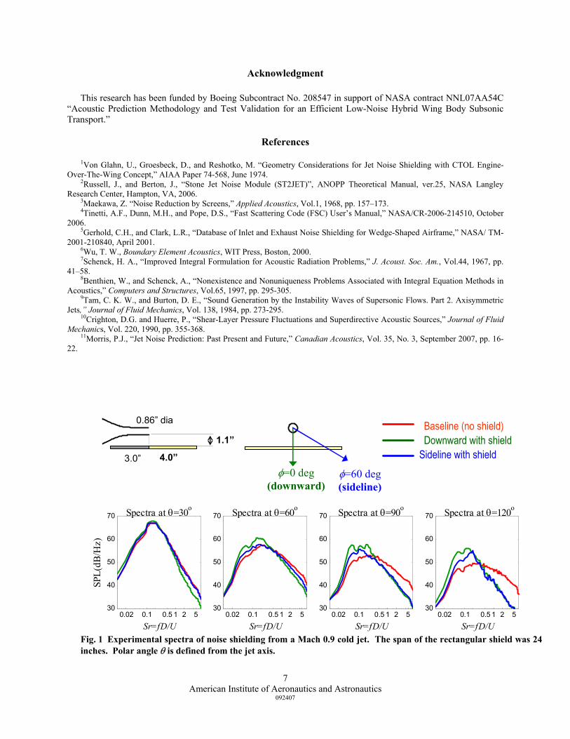
II. Some Experimental Data To appreciate the nature of jet noise shielding, it is instructive to examine some acoustic data involving simple jets and shields. As mentioned in the Introduction, significant experimental work on jet noise shielding occurred in the 1970s; however, the range and documentation quality of published data is not sufficient to develop a thorough understanding of the trends and accordingly develop prediction tools. For this reason we recently started a parametric experimental study of jet noise shielding in subscale aeroacoustic facilities at U.C. Irvine. Figure 1 shows narrowband sound pressure level spectra for one of the configurations tested. The spectra are plotted against Strouhal number Sr=fDj/Uj. With increasing polar angle θ from the jet axis shielding becomes more pronounced for Sr>0.5 but there substantial noise excess for Sr<0.5. This is consistent with trends observed in previous works. Earlier works attributed the excess noise to jet scrubbing the shielding surface. However for the experiment shown in Fig. 1 it was verified, using Pitot surveys, that the jet did not contact the shielding plate. The excess noise therefore is not necessarily connected to scrubbing and may also be caused by the jet noise source and its interaction with the surface. Any physical model should be able to predict not only the noise suppression but also the noise excess created by the “shield.” Models relying on point source approximation are bound to be unsatisfactory for two principal reasons: (a) for the point source, there is no distinction between near- and far-fields, whereas the jet pressure field is very different in the near field (where it interacts with the plate) than in the far field; (b) using point sources it would be difficult to include the directionality of the jet noise without making ad-hoc, empirical modifications. In this paper we will also present experimental data of a point source shielded by a plate. The point source was created by four impinging in an arrangement similar to that used by Gerhold and Clark.5

III. Boundary Element Method A schematic diagram for the boundary element acoustics is illustrated in Fig. 2. In the acoustic medium we have

a noise source S and a receiver R located at xS and xR respectively. The noise source can be a plane sound wave, a point source, or a distributed source. To reduce the noise exposure for the receiver, some kind of structure such as a panel is placed between the noise source and the receiver. We are primarily interested in how much noise can be reduced by the presence of the shielding panel. This basic model is used to study the shielding of jet engine noise by airframe structures. To study noise shielding by structures, the Helmholtz equation is to be solved,

2 2 0p k p∇ + = (1)


092407

2

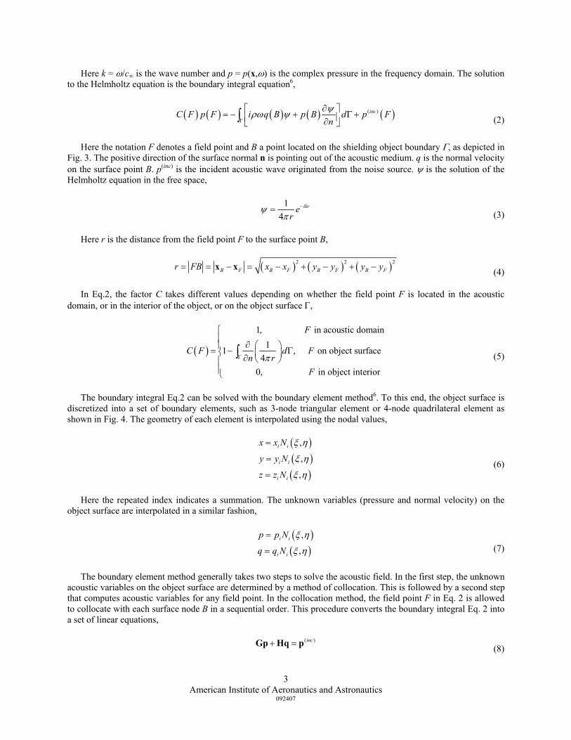
Here k = ω/c∞ is the wave number and p = p(x,ω) is the complex pressure in the frequency domain. The solution to the Helmholtz equation is the boundary integral equation6,

( ) ( ) ( ) ( ) ( )( )incC F p F i q B p B d p Fnψρω ψ

Γ

∂ = − + Γ + ∂ ∫ (2)

Here the notation F denotes a field point and B a point located on the shielding object boundary Γ, as depicted in Fig. 3. The positive direction of the surface normal n is pointing out of the acoustic medium. q is the normal velocity on the surface point B. p(inc) is the incident acoustic wave originated from the noise source. ψ is the solution of the Helmholtz equation in the free space,

1

4ikre

rψ

π−= (3)

Here r is the distance from the field point F to the surface point B,

( ) ( ) ( )2 2 2B F B F B F B Fr FB x x y y y y= = − = − + − + −x x (4)

In Eq.2, the factor C takes different values depending on whether the field point F is located in the acoustic domain, or in the interior of the object, or on the object surface Γ,

( )

1, in acoustic domain11 , on object surface

40, in object interior

F

C F d Fn r

FπΓ

∂ = − Γ ∂

∫ (5)

The boundary integral Eq.2 can be solved with the boundary element method6. To this end, the object surface is discretized into a set of boundary elements, such as 3-node triangular element or 4-node quadrilateral element as shown in Fig. 4. The geometry of each element is interpolated using the nodal values,

( )( )( )

,

,

,

i i

i i

i i

x x N

y y N

z z N

ξ η

ξ η

ξ η

=

=

= (6)

Here the repeated index indicates a summation. The unknown variables (pressure and normal velocity) on the object surface are interpolated in a similar fashion,

( )( )

,

,i i

i i

p p N

q q N

ξ η

ξ η

=

= (7)

The boundary element method generally takes two steps to solve the acoustic field. In the first step, the unknown acoustic variables on the object surface are determined by a method of collocation. This is followed by a second step that computes acoustic variables for any field point. In the collocation method, the field point F in Eq. 2 is allowed to collocate with each surface node B in a sequential order. This procedure converts the boundary integral Eq. 2 into a set of linear equations,

(8) ( )inc+ =Gp Hq p


092407

3

Here p and q are vectors of pressure and normal velocity variables respectively, and the coefficient matrices G and H are given by,

ij ij j

ij

ij ij j

G C N dn

H i N d

ψδ

ρω ψ

Γ

Γ

∂ = + Γ ∂

= Γ

∫

∫ (9)

For each surface node B, either the acoustic pressure or the normal velocity is given as a boundary condition. By moving the known terms to the right hand side and keeping the unknown variables on the left hand side, Eq. 8 can be written as,

=Ax b (10)

Here x is a vector of unknown variables (either pressure or normal velocity) on the object surface. At the natural resonant frequencies, Eq. 10 may become singular in an exterior scattering problem. To overcome this difficulty, some CHIEF (Combined Helmholtz Integral Equation Formulation) points may be used to introduce additional constraints in Eq. 107,8. Then the over-determined system of linear equations can be solved in a least square sense. With the acoustic variables solved for the object surface nodes, it is straightforward to compute the acoustic field by the use of the boundary integral equation (Eq.2). Next we present the verification of our BEM program on a benchmark scattering problem.

IV. Wavepacket Model for Jet Noise Jet noise sources are extremely complex and the subject of intense research and debate. It is generally agreed that

sound emission in the aft direction, at shallow angles to the jet axis, is caused by large-scale turbulent structures while noise emitted at large angles to the jet axis is caused by fine-scale turbulent motions. The large-scale structures can be modeled as instability waves that grow and then decay with axial distance. The resulting wavepacket model for jet noise stems from the seminal works by Tam and Burton9 and by Crighton and Huerre10 that have successfully captured salient elements of noise emission for jets and shear layers. Below we describe the wavepacket in its simplest axisymmetric form. More complex forms are possible by superposition of modes.

The jet is replaced by a cylinder r=r0 (for illustration see Fig. 10) on which we prescribe the pressure perturbation

(11) tiexptxrp ω−= )(),,( 00

Denoting the spatial Fourier transform of p0(x) as , the far-field solution for the pressure is)(ˆ0 kp 11

ticRi ee

rc

H

cp

RitRp ωω

θω

θω

πθ −

∞

∞ ∞

−= /

0)1(

0

0

sin

cosˆ),,( (12)

Specifically for a Gaussian wavepacket, the prescribed pressure has the form

(13) xixxbxi eeexAxp αα ε

20 )(

0 )()( −−==

whose Fourier transform is


092407

4

bkxki ee

bkp 4/)()(

0

20)(ˆ ααπε −−−= (14)

Important quantities with respect to noise emission are the convective Mach number Mc=ω/(αc∞) and the width of the Gaussian envelope controlled by b. For the case computed here, Mc=0.71, x0=0, and b=461 m-2, corresponding to an envelope length (down to 1% of peak amplitude) of 0.2 m. We select frequencies according to the Strouhal number Sr=ωDj/(2πUj) where Dj=2r0=0.02 m is the jet diameter and Uj=350 m/s is the jet exit velocity. Values of Sr around 0.1 to 0.2 correspond to peak noise emission. The convective velocity Uc=ω/α is assumed to be 70% of the jet exit velocity Uj.

V. Verification of BEM Program To study noise shielding by general airframe structures, we have developed a computer program to implement

the boundary element method. Before the BEM program is used for study of acoustic shielding, it must be verified on benchmark test examples. One such standard test example is the acoustic scattering of a plane wave by a rigid sphere, for which there is an analytical solution to compare with.

Figure 5 shows a schematic diagram of a plane acoustic wave passing around a rigid sphere of radius a. With the time harmonic factor eiωt omitted in relevant expressions, the incident pressure wave can be written as,

( ) ( ) (( ) cos

02 1 cosinc ikz ikr m

m mm

p e e m i j kr Pθ )θ∞

=

= = = +∑ (15)

Here θ is the polar angle, i is the complex number unit, jm is the m-th order spherical Bessel function, and Pm is the m-th order Legendre function. The scattered pressure field is,

( ) ( )( ) ( ) ( )( ) (1)

(1)0

2 1 cosmsca mm m

m m

j kap m i h kr P

h kaθ

∞

=

′= + − ′ ∑ (16)

Here h(1) is the spherical Hankel function of first kind. The superscript prime in Eq. 16 denotes differentiation with respect to the argument. The total acoustic field is the summation of the incident field and the scattered field.

This analytical solution is used to check the accuracy of the numerical results from the BEM program. Two cases are considered here. The first case is for a fixed frequency that corresponds to a wavenumber parameter of ka=10. We look at the total pressure values for field points located on a measurement circle on the yz-plane as depicted in Fig. 5. Specifically, we take the radius of the measurement circle to be Rm = 3a. The comparison between the BEM result and the analytical solution is shown in Fig. 6, where the total pressure amplitude is plotted out against polar angles varying from 0° to 180°. The agreement between these two approaches is excellent.

The second case is to look at a fixed field point with noise source frequencies varied. The field point is chosen to be point F on the measurement circle. Its polar coordinates are (Rm, θ) = (3a, 180). The result of the total pressure amplitude as a function of ka is shown in Fig. 7. Again the BEM result has a good agreement with the exact solution. This verifies the accuracy of our BEM computer program. Next we will use the BEM program to study noise shielding of point sources by airframe structures such as a panel structure.

VI. Numerical Results on Noise Shielding With the BEM program verified, we now look at some numerical examples. Shielding will be quantified in terms

of the insertion loss (IL), which is defined as,

2( )

10 ( )10 logWIP

WOP

pILp

= − (17)

Here p(WIP) refers to the pressure value with the panel in place, and p(WOP) is the pressure value without the panel in place. For a given source-shield arrangement, the insertion loss is a function of both the location of the receiver and the frequency of the noise source.


092407

5

Our first computational case is the noise shielding of a point source by a panel structure. The panel size is 24 in × 7 in × 1/8 in as depicted in Fig. 8. The origin O of the coordinate system xyz coincides with the center of the panel. A point noise source is located above the panel off the center by a distance of 1.25in, i.e., the coordinate of the point source is (0 in. , 0 in. , 1.25 in.). The receiver is located at the point (0 in., 0 in., -39 in.). Figure 9 plots the insertion loss as a function of frequency for this receiver. Shown are the results of the BEM computation, Maekawa’s empirical formula, and experimental data. There is general agreement in the trends of all three types of data, although Maekawa’s formula overestimates the insertion loss. Comparison between with experiment and BEM is good except at very low frequency where the experimental insertion loss shows a spike. One should keep in mind that the experimental source is not a perfect point source (it has a small but finite volume) and that the experimental distances could be off by a few percent. Nevertheless, the agreement of BEM with experiment is encouraging.

The next case is the wavepacket of Section IV and its interaction with a solid surface. The computational setup is depicted in Fig. 10. The shielding plate has dimensions of 0.2 m × 0.6 m × 0.01 m and is placed 0.04 m below the jet axis. We first examine the far-field pressure of the wavepacket alone and compare it to the analytical solution (Eq.12). For the BEM computation, the wavepacket cylinder must be truncated to a finite length, whereas in the theoretical model the cylinder extends to ±∞ in the axial direction. In this computation the wavepacket length was 0.80 m. The pressure on the cylinder surface is prescribed as a Gaussian distribution defined by Eq. 13. The “active” part of the wavepacket (down to 1% of peak amplitude) occupies the central 0.2 m of its total length. The plot of the pressure amplitude on the wavepacket surface is depicted in Fig. 11. Given the narrow region of the peak pressure value, it is important to use sufficient number of mesh points to resolve the Gaussian distribution. We checked grid convergence by using two types of meshes as shown in Fig. 12. One was a uniform mesh and the other was non-uniform mesh with more mesh points concentrated in the center region. We obtained essentially the same simulation results from these two mesh sizes, indicating the BEM result is convergent and mesh-independent. Figure 13 shows the plot of pressure amplitude at an observation radius of R=1 m for variable polar angle. BEM predictions for two Strouhal numbers, Sr=0.1 and 0.2, were computed and compared with the corresponding analytical solutions. The agreement of BEM prediction and theory is very good overall. At low polar angles there are small deviations due to the finite axial extent of the computational wavepacket.

We then insert a plate barrier as depicted in Fig. 10. The span of the barrier is 0.6 m and the thickness is 0.02 m. The resulting insertion loss versus polar angle for Sr=0.1 is plotted in Fig. 14. At low polar angles, the barrier causes noise suppression. As we increase the polar angle, we observe amplification in pressure level, manifested as a negative insertion loss. While this result may be surprising at first, it is consistent with the experimental measurements of Fig. 1. A possible physical explanation is a follows: the jet noise source (simulated here by the wavepacket) is highly directional, with intense radiation at shallow angles to the jet axis and weak radiation at large polar angles, as shown in Fig. 12. Inserting a barrier in the manner shown in Fig. 10, a significant portion of the high-intensity sound is diffracted around the trailing edge and directed toward the “quiet” region. This causes amplification in sound pressure level at the high polar angles. We expect this phenomenon to be dominant at low frequencies for which the extent of the source is large relative to the barrier size. As the frequency increases, the source becomes more compact and thus better shielded by the barrier. At this point, our computations resolved only Sr=0.1. Computation at high Sr, for which we expect sound suppression, will require large computational resources which we hope to have available in the near future. For now it appears that the wavepacket model captures a key element of jet noise shielding that cannot be predicted using point source models.

VII. Conclusion This study has been motivated by the need of reliable and physics-based prediction methods for jet noise

shielding. The success of such methods is inextricably connected to the proper description of the jet noise source. We seek a computational approach that facilitates the exploration of various jet noise source models and their eventual comparison to experimental results. The Boundary Element Method (BEM) provides such an approach. We use BEM to test a variety of noise source models, in combination with shields, to understand the salient physics of the problem and develop predictive methodologies. These methodologies will not be inherent to BEM and could be incorporated in other computational methods. In this paper, we first validated the BEM against the classical solution for plane wave diffraction around a sphere. Then we computed the problem of a point source shielded by a rectangular plate. The computed insertion loss is in good agreement with experimental data. Finally we simulated jet noise using a wavepacket model and examined its interaction with a plate barrier. We observed amplification (instead of suppression) of sound pressure level at low frequency, which is consistent with experimental data and cannot be readily explained by point source approximation of jet noise.


092407

6

Acknowledgment This research has been funded by Boeing Subcontract No. 208547 in support of NASA contract NNL07AA54C

“Acoustic Prediction Methodology and Test Validation for an Efficient Low-Noise Hybrid Wing Body Subsonic Transport.”

References 1Von Glahn, U., Groesbeck, D., and Reshotko, M. “Geometry Considerations for Jet Noise Shielding with CTOL Engine-

Over-The-Wing Concept,” AIAA Paper 74-568, June 1974. 2Russell, J., and Berton, J., “Stone Jet Noise Module (ST2JET)”, ANOPP Theoretical Manual, ver.25, NASA Langley

Research Center, Hampton, VA, 2006. 3Maekawa, Z. “Noise Reduction by Screens,” Applied Acoustics, Vol.1, 1968, pp. 157–173. 4Tinetti, A.F., Dunn, M.H., and Pope, D.S., “Fast Scattering Code (FSC) User’s Manual,” NASA/CR-2006-214510, October

2006. 5Gerhold, C.H., and Clark, L.R., “Database of Inlet and Exhaust Noise Shielding for Wedge-Shaped Airframe,” NASA/ TM-

2001-210840, April 2001. 6Wu, T. W., Boundary Element Acoustics, WIT Press, Boston, 2000. 7Schenck, H. A., “Improved Integral Formulation for Acoustic Radiation Problems,” J. Acoust. Soc. Am., Vol.44, 1967, pp.

41–58. 8Benthien, W., and Schenck, A., “Nonexistence and Nonuniqueness Problems Associated with Integral Equation Methods in

Acoustics,” Computers and Structures, Vol.65, 1997, pp. 295-305. 9Tam, C. K. W., and Burton, D. E., “Sound Generation by the Instability Waves of Supersonic Flows. Part 2. Axisymmetric

Jets,” Journal of Fluid Mechanics, Vol. 138, 1984, pp. 273-295. 10Crighton, D.G. and Huerre, P., “Shear-Layer Pressure Fluctuations and Superdirective Acoustic Sources,” Journal of Fluid

Mechanics, Vol. 220, 1990, pp. 355-368. 11Morris, P.J., “Jet Noise Prediction: Past Present and Future,” Canadian Acoustics, Vol. 35, No. 3, September 2007, pp. 16-

22.

Baseline (no shield)Downward with shield

Sideline with shieldφ=0 deg

(downward)

4.0”

1.1”

3.0”

0.86” dia

φ=60 deg(sideline)

0.02 0.1 0.5 1 2 530

40

50

60

70

SPL(

dB/H

z)

Sr=fD/U

Spectra at θ=30o

0.02 0.1 0.5 1 2 530

40

50

60

70

Sr=fD/U

Spectra at θ=60o

0.02 0.1 0.5 1 2 530

40

50

60

70

Sr=fD/U

Spectra at θ=90o

0.02 0.1 0.5 1 2 530

40

50

60

70

Sr=fD/U

Spectra at θ=120o

Fig. 1 Experimental spectra of noise shielding from a Mach 0.9 cold jet. The span of the rectangular shield was 24inches. Polar angle θ is defined from the jet axis.


092407

7

Fig. 2 Schematic diagram of t from the source point S towar

AcAc

Fig. 3 Diagram showing a fielscattering problem, the positiv

Am

S ( ), ,S S S Sx y z=x

R ( ), ,R R R Rx y z=x

y

x

z

panel

S ( ), ,S S S Sx y z=x

R ( ), ,R R R Rx y z=x

y

x

z

panel

he noise shielding problem. A structural panel is used to shield the noise originatedd receiver R.

B

F

n

Γ

S

Object interior

oustic medium ( )incp

B

F

n

Γ

S

Object interior

oustic medium ( )incp

d point F, a surface node B on the object surface boundary Γ. In an exterior e direction of the surface normal n is pointing out of the acoustic domain.

erican Institute of Aeronautics and Astronautics

092407

8

Fig. 4 Bilinea

\

Fig.5 Diagram showing radius Rm is drawn on th

x

y

z

a mR

( )inc ikz i tp e e ω=

F θ

an acoustic plane wave impinging on a rigid sphere of radius a. A measurement circle of

x

y

z

ξ

η

(1) (2)

(3)(4)

( )( )( )

,

,

,

i i

i i

i i

x x N

y y N

z z N

ξ η

ξ η

ξ η

=

=

=

Quadrilateral Master element

(1) (2)

(3)(4)

-1

-1

1

1

( ) ( )( ) ( )( ) ( )( ) ( )

1

2

3

4

1 1 4

1 1 4

1 1 4

1 1 4

N

N

N

N

ξ η

ξ η

ξ η

ξ η

= + +

= − +

= − −

= + −

x

y

z

ξ

η

(1) (2)

(3)(4)

( )( )( )

,

,

,

i i

i i

i i

x x N

y y N

z z N

ξ η

ξ η

ξ η

=

=

=

Quadrilateral Master element

(1) (2)

(3)(4)

-1

-1

1

1

( ) ( )( ) ( )( ) ( )( ) ( )

1

2

3

4

1 1 4

1 1 4

1 1 4

1 1 4

N

N

N

N

ξ η

ξ η

ξ η

ξ η

= + +

= − +

= − −

= + −

r interpolation for a quadrilateral element.

e yz-plane. A field point F is also shown on the measurement circle at polar angle θ.


092407

9

Fig. 6 Plot of pressure amplitude versus polar angle θ on the measurement circle for plane wave diffracted by sphere. Wave number parameter ka=10.

Fig. 7 Plot of pressure amplitude versus wave number parameter ka for plane eave diffraction by sphere. The field point F is located on the measurement circle at θ=180 deg.


092407

10

Fig. 8 Sche point sourc

Fig. 9 Plot

1/8"

7"

24"

x

y

z

1.25"

39"

Point source

Receiver

ikr1p = e4πr

O

1/8"

7"

24"

x

y

z

1.25"

39"

Point source

Receiver

ikr1p = e4πr

O

matic diagram of noise shielding by a panel structure. Panel size is 24” × 7” × 1/8”. Thee and the receiver are located right above and below the center of the panel, respectively.

-5

0

5

10

15

20

25

0 2000 4000 6000 8000 10000

f (Hz)

Inse

rtion

Los

s (dB

)

BEMExperimentMaekawa

of insertion loss versus frequency for point source and rectangular plate arrangement of Fig. 8.


092407

11

x

r

r0=0.010 mθ

ys=0.040 m

R = 1.000 mxs=0.200 m

x0=0

Fig. 10 Illustration of wavepacket model for jet noise and shielding setup

Fig. 11 directio

(a) (b)(a) (b)

Distribution of pressure amplitude on wavepacket cylinder. (a) Contour plot on cylinder surface. Radialn is scaled up for better visualization; (b) pressure profile on surface.


092407

12

(a) (b)(a) (b)

Fig. 12 Computational mesh used for wavepacket cylinder. The radial direction is scaled up 20 times for better visualization. (a) Uniform mesh; (b) non-uniform mesh.

Fig. 13 Far-field pressure of wavepacket without shielding. Comparison of the BEM prediction with analytical solution.


092407

13

-8.0

-6.0

-4.0

-2.0

0.0

2.0

4.0

6.0

30 60 90 120 150 180θ (deg)

Inse

rtion

Los

s (dB

)

Sr =0.1

Fig. 14 Insertion loss prediction of BEM for the interaction of wavepacket with plate at Sr=0.1.


092407

14

numerical study of noise shielding by airframe...

Documents