o shoring, exporting, and jobs - home | economics | uci
TRANSCRIPT
Offshoring, Exporting, and Jobs
Jose L. GroizardDepartament d’Economia Aplicada
Universitat de les Illes Balears
Priya Ranjan∗
Department of EconomicsUniversity of California, Irvine
Antonio Rodriguez-LopezDepartment of Economics
University of California, Irvine
October 2013
Abstract
We construct a two-sector model—one producing a homogeneous good and the other pro-ducing differentiated goods—with labor market frictions to study the impact of offshoring onintrafirm, intrasectoral, and intersectoral reallocation of jobs, and on the economy-wide unem-ployment rate. A reduction in the offshoring cost affects intrafirm and intrasectoral reallocationin the differentiated-good sector through a job-relocation effect, a productivity effect, and acompetition effect. The key parameters determining the impact of offshoring on reallocation ofjobs at various margins as well as on the economy-wide unemployment rate are the elasticityof substitution between inputs and the elasticity of demand for differentiated goods. Allowingdifferentiated-good firms to export creates an additional channel through which a reduction inthe cost of offshoring affects jobs and unemployment. We also show that the implications ofa reduction in the cost of trading final goods are different from those of a reduction in theoffshoring cost.
JEL Classification: F12, F16
Keywords: heterogeneous firms, offshoring costs, search frictions, unemployment
∗Corresponding author. Department of Economics, University of California, Irvine. Address: 3151 Social SciencePlaza, Irvine, CA 92697-5100, USA. Telephone number: +1 (949) 824-1926. Fax number: +1 (949) 824-2182. E-mail:[email protected].
1 Introduction
Offshoring refers to the relocation of a part of the production process abroad either within the firm’s
boundary or through arm’s length trade. Since the relocation of the production process goes hand
in hand with the relocation of jobs, it gives rise to the fear—fed by media stories—that there are
job losses in the country whose firms engage in offshoring.1 Not only has this caused anxiety among
the public at large, but politicians in the U.S. (on both sides of the aisle) and Europe have done
fear-mongering regarding offshoring.2 This has also given rise to calls to throw sand in the wheels
of offshoring to stem job losses. However, this simplistic story ignores the various channels through
which offshoring can affect jobs. Before implicating offshoring as the main source of job losses,
we need to understand its overall employment effects and not just the immediate job-relocation
effect. This paper constructs a two-sector theoretical model with labor market frictions to identify
the channels through which offshoring affects job flows (at the firm and industry levels) and the
economy-wide unemployment rate.
In our set up, one sector produces a homogeneous good using only domestic labor. The other
sector has heterogeneous firms producing differentiated goods. The differentiated-good firms use a
continuum of intermediate inputs, which are combined using a constant elasticity of substitution
(CES) production function. The production of each intermediate input can be either offshored
or undertaken using domestic labor, but offshoring is subject to heterogeneous costs a la Gross-
man and Rossi-Hansberg (2008). There are search frictions in both sectors affecting the hiring of
domestic workers. Workers are mobile across sectors but because of differences in search parame-
ters, unemployment rates and wages differ across sectors. The economy-wide unemployment rate
depends on both the sectoral unemployment rates as well as on the share of workers in each sector.
We show that a decrease in the variable cost of offshoring affects employment in the differentiated-
good sector not only by affecting employment at the firm level, but also through changes in the
number of firms. Following a reduction in the variable cost of offshoring, offshoring firms increase
the fraction of inputs they offshore, which reduces their domestic employment. We call this the
job-relocation effect. But also, offshoring firms become more productive as a result of lower input
costs, which allows them to charge a lower price. Whether the resultant increase in demand for their
1For example, The Economist (Jan 19th, 2013) says: “But offshoring from West to East has also contributed tojob losses in rich countries, especially for the less skilled, yet increasingly for the middle classes too... In a survey byNBC News and the Wall Street Journal in 2010, 86% of Americans polled said that offshoring of jobs by local firmsto low-wage locations was a leading cause of their country’s economic problems.”
2The same article in The Economist above notes: “Barack Obama’s presidential campaign last year repeatedlyclaimed that his rival, Mitt Romney, had sent thousands of jobs overseas when he was working in private equity.Mr Romney, in turn, attacked Chrysler, a car firm, for planning to make Jeeps in China. France’s new Socialistgovernment has appointed a minister, Arnaud Montebourg, to resist ‘delocalisation’. Germany’s chancellor, AngelaMerkel, worries publicly about whether the country will still make cars in 20 years’ time.”
1
products translates into higher domestic employment depends on two parameters: the elasticity of
substitution between differentiated-good varieties and the elasticity of substitution between inputs.
We call this the productivity effect of offshoring on employment. Lastly, a decline in the cost of
offshoring makes the competitive environment tougher, leading to a reduction in the demand faced
by individual firms. We call this last effect the competition effect of offshoring.
For offshoring firms, the job-relocation and competition effects reduce domestic employment,
while the productivity effect—assuming the elasticity of substitution between varieties is higher than
the elasticity of substitution across inputs—increases domestic employment. Since non-offshoring
firms experience only the competition effect, they reduce their employment. A decline in offshoring
costs leads to an increase in the mass of offshoring firms, but the impact on the overall mass
of firms in the differentiated-good sector is ambiguous. Combining the effects at the intensive
and extensive margins, the net effect of a decline in the offshoring cost on employment in the
differentiated-good industry depends on two key parameters: the elasticity of substitution between
inputs and the elasticity of demand for differentiated goods.3 A low value of the former is more
conducive to net job creation—a value below 1 implies complementarity between offshored inputs
and domestic labor. Similarly, a high value of the latter—implying a greater increase in the demand
for differentiated goods following a reduction in offshoring costs—is more likely to lead to net job
creation. We provide numerical examples to highlight the key results.
How these employment changes affect the economy-wide rate of unemployment depends on
two factors: the degree of search frictions in each sector and the change in the composition of
the workforce. If the degree of search frictions is higher in the differentiated-good sector then
the unemployment rate is higher there as well. Now, if in response to a decrease in the cost of
offshoring there is a decline in employment in the differentiated-good sector—so that workers move
to the (lower unemployment) homogeneous-good sector—then the economy-wide unemployment
rate would decline. In the opposite case where workers move to the differentiated-good sector, the
economy-wide unemployment rate increases.
Our model also allows us to study the implications of changes in search frictions. For example,
a decrease in search frictions in the differentiated-good sector makes it cheaper to hire domestic
labor in that sector and consequently offshoring declines. Therefore, the impact on firm-level
employment is similar to that of an increase in the cost of offshoring with one difference: there is
an additional positive effect on the employment of all firms because the marginal cost of production
for all differentiated-good firms declines. Regarding the economy-wide unemployment rate, there
3By extensive margin, we refer to changes in employment due to entry and exit of firms. On the other hand, byintensive margin we mean employment changes due to expansions and contractions of existing firms.
2
are two forces at work. While the composition of the labor force matters, as was the case when the
offshoring cost changed, now the unemployment rate in the differentiated-good sector declines as
well, which would tend to reduce the economy-wide unemployment rate.
The model described above does not allow differentiated-good firms to export. However, an
important stylized fact in micro-level data is that importing of inputs and exporting go hand in
hand in many firms. For example, Bernard, Jensen, and Schott (2009) document that 42% of the
U.S. civilian employment at private firms was in trading firms, while 30% of the employment was
at the firms that do both export and import. As well, Bernard, Jensen, Redding, and Schott (2007)
show that 79% of firms in the U.S. that import also export. In an important extension of our basic
model, we show how offshoring can increase exporting and thereby be an important source of job
creation for trading firms.
We extend the model to a North-South world where our original country, the North, offshores
some inputs to the South and the differentiated-good producers in both countries can export to
each other. The South has a comparative advantage in producing inputs and hence, while the two
countries are symmetric with respect to exporting, only the North offshores. In this setting it is
shown that a decrease in the cost of offshoring makes the Northern firms more productive relative
to the Southern firms in both markets. As a consequence, the numbers of entrants and exporting
firms increase in the North, which leads to net job creation at the extensive margin—in the absence
of exporting opportunities, there is no guarantee of net job creation at the extensive margin. At
the intensive margin, in addition to the job relocation, productivity, and competition effects arising
from Northern firms’ sales to their domestic market, these effects arise as well for Northern firms’
export sales. While the job-relocation and productivity effects for export sales are similar to those
for domestic sales, the competition effect in the export market is different. In particular, while
the competition effect relevant for domestic sales leads to job destruction, the competition effect
relevant for exports leads to job creation. This offshoring-induced job creation due to exporting
possibilities increases the likelihood that the overall effect of offshoring on differentiated-good sector
employment is positive.
The impact on the economy-wide unemployment rate depends again on the composition of the
workforce and the extent of search frictions in the two sectors. The extended model also allows
us to do comparative statics with respect to the trading cost of differentiated goods. One notable
result compared to the case of a change in the offshoring cost is the absence of job-relocation and
productivity effects. In fact, we show that a decline in the offshoring cost and a decline in the cost
of trading differentiated goods can have opposite effects on the economy-wide unemployment rate.
Lastly, the two trading costs interact in significant ways: the impact of a decrease in the cost of
3
trading differentiated goods on job flows is larger the smaller the offshoring cost and vice-versa.
Irrespective of its impact on unemployment, offshoring always increases welfare. Intuitively,
offshoring always leads to productivity improvements for the economy, which shows up in the form
of a decline in the differentiated-good price index and, consequently, in an increase in welfare.
Given our simplifying assumption of a representative household which diversifies away labor in-
come risk, everyone gains from offshoring. However, this result needs to be treated with caution
because in reality labor income risks are unlikely to be diversified away completely, and therefore,
unemployed individuals are necessarily worse off than employed individuals; if offshoring increases
unemployment, it necessarily makes some people—the newly unemployed—worse off.
1.1 Related Literature
Our modeling of offshoring by heterogeneous firms is informed by stylized facts. In our model
there is a fixed cost of offshoring, a feature that we share with the workhorse offshoring model
of Antras and Helpman (2004). An implication is that only the most productive firms offshore,
which is consistent with the stylized fact that importing firms are on average more productive
and larger than purely domestic firms (see, e.g., Bernard, Jensen, Redding, and Schott, 2007 for
the U.S.). We go beyond Antras and Helpman (2004) in postulating a production function with a
continuum of inputs with the set of offshored inputs being determined endogenously and responding
to changes in offshoring costs. This is consistent with the evidence in Goldberg, Khandelwal,
Pavcnik, and Topalova (2010) who find that a decline in input trade costs expands the set of
imported intermediate inputs for Indian firms, which then translates into an increase in the number
of final products they produce. Similarly, Gopinath and Neiman (2013) show that a large part of
the import adjustment in response to a large currency depreciation in Argentina took the form
of a decline in the number of imported inputs at the firm level. This channel, which Gopinath
and Neiman (2013) call the sub-extensive margin, can explain 45% of the decline in Argentina’s
imports, and is also responsible for the decline in firm-level productivity. Hence, their evidence is
also supportive of the offshoring productivity effect obtained in our model.4
Empirical evidence also suggests that complementarity/substitutability between inputs may
be crucial in determining the labor market implications of offshoring. Therefore, we use a CES
production function which allows us to study how the impact of offshoring depends on the elasticity
of substitution (or complementarity) among inputs. Using data on the U.S. multinationals, Harrison
and McMillan (2011) find that when the tasks performed by the subsidiary of a multinational
4There is further empirical support for the impact of offshoring on firm productivity. For example, Amiti andKonings (2007) (for Indonesia) and Topalova and Khandelwal (2011) (for India) find the positive effect of lower inputtariffs on productivity to be much stronger than the effect lower output tariffs.
4

are complementary to the tasks performed at home, offshoring leads to more job creation in the
United States; however, offshoring causes job losses when the tasks performed in the subsidiary
are substitutes for the tasks performed at home. This is consistent with our theoretical result that
offshoring is more likely to cause job creation via the productivity effect if inputs are complementary.
Our paper is related to the growing literature on the impact of globalization on labor markets
with search frictions. Pioneers of this literature are Carl Davidson and Steven Matusz, who in
a series of papers study the implications of introducing unemployment arising from labor market
frictions in trade models. As discussed in Davidson and Matusz (2004), their work has focused
more on the roles of efficiency in job search, the rate of job destruction, and the rate of job
turnover in the determination of comparative advantage. Moore and Ranjan (2005) show how
trade liberalization in a skill-abundant country can reduce the unemployment of skilled workers
and increase the unemployment of unskilled workers. Since each sector employs only one type
of labor, there is no intersectoral reallocation of labor. Felbermayr, Prat, and Schmerer (2011)
study the impact of a reduction in the cost of trading final goods on unemployment in a one-sector
model with firm heterogeneity. Since their model has only one sector, there is no intersectoral
reallocation of labor there either. Neither of these papers studies the implications of offshoring on
unemployment.
Our structure with a homogeneous-good sector and a differentiated-good sector—with firm
heterogeneity in the latter—is similar to the structure of Helpman and Itskhoki (2010), as is the
use of a static model of search frictions. One difference in the modeling of labor market frictions
is that while wages are determined by multilateral bargaining in the Helpman-Itskhoki model, we
use the competitive-search approach of Shimer (1996) and Moen (1997) where firms post wages
and workers direct their search. The most important difference, however, is that our main interest
lies in studying the implications of offshoring on unemployment, while they study the implications
of trade liberalization in final goods. To this end, we use a production function for firms in the
differentiated-good sector which uses a continuum of inputs with heterogeneous offshoring costs.
As a result, we identify some channels of influence such as the job-relocation effect, the productivity
effect, and the domestic- and export-market competition effects, which arise due to the offshoring
structure of our model. In the extension with differentiated-good trade we also provide comparative
statics with respect to a decrease in the cost of trading final goods and obtain results similar to
Helpman-Itskhoki. We also show that a decrease in the offshoring cost can lead to a very different
intersectoral reallocation of resources compared to a decrease in the trading cost of final goods.
Mitra and Ranjan (2010) study the impact of offshoring on unemployment in a two-sector model
similar to ours where firms in one of the two sectors offshore. Their offshoring structure is much
5
simpler, with perfectly competitive firms producing with two inputs, only one of which can be
offshored. Our production structure with a continuum of inputs with all of them being potentially
offshorable—with the fraction of offshored inputs depending on offshoring costs—is more general.
As well, the introduction of firm heterogeneity allows us to obtain the implications of offshoring
at both the intensive and extensive margins. Ranjan (2013) studies the role of wage-bargaining
institutions in determining the impact of offshoring on unemployment. Neither of these papers has
firm heterogeneity and therefore, cannot study the heterogeneous response of firms to a change
in the cost of offshoring. Davidson, Matusz, and Shevchenko (2008) also study the implications
of offshoring in a job-search model with the focus on the offshoring of high-tech jobs on low- and
high-skilled workers’ wages, and on overall welfare.
A related recent paper by Egger, Kreickemeier, and Wrona (2013) also studies the implications
of offshoring in a model with firm heterogeneity. Their focus is on the implications of offshoring
for inequality in the distribution of income, both within and between entrepreneurs and workers.
They extend the model to allow for unemployment, which in their setting is driven by fair-wage
considerations. Their Cobb-Douglas production function, same as in Antras and Helpman (2004),
restricts the model to the case of unitary elasticity of substitution between domestic labor and
offshored inputs. In our set up, unemployment arises due to search friction and our CES produc-
tion function with a continuum of inputs allows us to study different degrees of substitution and
complementarity between domestic labor and offshored inputs. As well, none of the papers on
offshoring and unemployment account for the link between offshoring and exporting activities of
firms, which is a novel feature of our paper.
The offshoring structure in our model is related to the trade-in-tasks structure of the model
of Grossman and Rossi-Hansberg (2008). While Grossman and Rossi-Hansberg (2008) assume
perfect complementarity between tasks, we use a CES production function and show how the
results depend crucially on the elasticity of substitution between inputs.5 Also, Grossman and
Rossi-Hansberg (2008) do not have labor market frictions and they do not consider either firm het-
erogeneity or exporting possibilities. Bernard, Redding, and Schott (2007) address the predictions
of final-good trade liberalization on gross job flows in their Heckscher-Ohlin model with Melitz-type
firm heterogeneity; however, neither do they have any labor market frictions, nor do they study
the impact of offshoring.
There is a growing empirical literature dealing with the impact of offshoring on employment,
which is the main concern of our paper. The evidence is mixed. Gorg (2011) provides a compre-
5By assuming perfect complementarity between tasks, Grossman and Rossi-Hansberg (2008) work with the specialcase in which the offshoring productivity effect is maximum.
6
hensive survey of this literature.6
Note that none of the above papers explicitly takes into account the possibility of offshoring
creating jobs through the export channel identified in our theoretical framework. However, the
positive effect of offshoring on employment found in many papers is consistent with the job creating
effects of offshoring through exporting. There are some papers which look at the impact of exporting
on employment without establishing a causal link between offshoring and the exporting activities
of a firm. Biscourp and Kramarz (2007) find that exporting has a positive impact on job growth in
French firms while importing has a negative effect on job growth. Using firm-level data from the
U.S., Davidson and Matusz (2005) find that net exports are positively associated with job creation.
Lastly, using a matched employer-employee data from Denmark, Hummels, Jorgensen, Munch,
and Xiang (2011) find that exporting is positively associated with employment but offshoring is
negatively associated with employment. Our theoretical framework suggests a causal link between
offshoring and exporting; that is, it is possible that some of the positive effect of exporting on
employment can be ascribed to offshoring by firms.
2 The Model
In this section we present our model with labor market frictions, heterogeneous firms, and het-
erogeneous offshoring costs. The model assumes a country with two sectors: a differentiated-good
sector and a homogeneous-good sector. Production in the homogeneous-good sector uses only do-
mestic labor, but heterogeneous firms in the differentiated-good sector can offshore a fraction of
their inputs.
We begin by defining preferences and demand, then we discuss our search approach for the labor
market, and describe the homogeneous- and differentiated-good sectors, with special attention on
differentiated-good firms’ offshoring decisions. Lastly, we define the equilibrium of this model and
describe how the economy-wide unemployment rate is determined.
2.1 Preferences and Demand
The country is populated by a continuum of households in the unit interval. Households’ preferences
are defined over a continuum of differentiated goods and a homogeneous good. Following Helpman
and Itskhoki (2010), we assume that the utility function for the representative household is given
by
U = H +η
η − 1Zη−1η , (1)
6See the discussion of following works in Gorg (2011): Gorg and Hanley (2005) for Ireland, Ibsen, Warzynski,and Westergard-Nielsen (2010) for Denmark, Amiti and Wei (2005) for the U.K., Amiti and Wei (2009) for the U.S.,Hijzen and Swaim (2007) for a multi-country study, and Wagner (2011) for Germany.
7
where H denotes the consumption of the homogeneous good, Z =(∫
ω∈Ω zc(ω)
σ−1σ dω
) σσ−1
is the
CES consumption aggregator of differentiated goods, and η > 1 is the elasticity of demand for Z (η
governs the substitutability between homogenous and differentiated goods).7 In Z, zc(ω) denotes
the consumption of variety ω, Ω is the set of differentiated goods available for purchase, and σ > 1
is the elasticity of substitution between differentiated-good varieties. It is assumed that σ > η so
that differentiated-good varieties are better substitutes for each other than for the homogeneous
good. The homogeneous good is the numeraire—its price is 1.
For differentiated goods, the representative household’s demand for variety ω is given by zc(ω) =
p(ω)−σ
P 1−σ PZ, where p(ω) is the price of variety ω, P =[∫ω∈Ω p(ω)1−σdω
] 11−σ is the price of the CES
aggregator Z, and hence, PZ is the aggregate spending on differentiated goods. Given the quasi-
linear utility function in (1), it follows that Z = P−η, and therefore, the demand for variety ω can
be rewritten as
zc(ω) = p(ω)−σP σ−η. (2)
It follows that the representative household spends p(ω)zc(ω) = p(ω)1−σP σ−η on this variety.
The representative household spends its labor income, E, on homogeneous and differentiated
goods. Given the quasi-linearity in (1), it follows that amount E−PZ = E−P 1−η is spent on the
homogeneous good. Therefore, the indirect utility function is given by
V = E +P 1−η
η − 1, (3)
which is increasing in spending, E, and decreasing in the differentiated-good price index, P . Given
that there is a unit measure of identical households, equation (2) is also the market demand, E is
equivalent to the total labor income in the economy, and PZ is the country’s total expenditure on
differentiated goods.
2.2 Labor Market and Search Frictions
As in Helpman and Itskhoki (2010), each household is composed of a fixed supply of L workers,
with each member willing to devote one unit of labor to production activities in either sector. Given
that households are located in the unit interval, the total size of the country’s workforce is also L.
We assume free mobility of workers across sectors.
Labor markets in both sectors are characterized by search frictions. While search frictions
are traditionally introduced in a dynamic framework, Helpman and Itskhoki (2010) convincingly
showed that the key insights in a model of trade with search frictions can be as easily generated
7The qualitative results of this paper would be unchanged with a homothetic utility function (however, the algebrabecomes tedious). The Appendix in Helpman and Itskhoki (2010) provides an outline of how to handle the case ofhomothetic utility.
8
using a static framework, and this is the approach we adopt. In our description of the labor
market, the only difference from Helpman and Itskhoki (2010) is in wage setting: while they
assume a multilateral-bargaining approach, we use the competitive-search approach pioneered by
Shimer (1996) and Moen (1997) where firms post wages and workers direct their search.8
Firms post vacancies and wages to attract workers. Higher wages attract more workers, requiring
less vacancies for each worker that a firm intends to hire. We assume that each firm j in sector
i, for i ∈ H,Z, decides to post a vacancy in a sub-market ij. Denote the number of vacancies
posted by a firm j in sector i by Vij , and the number of applicants attracted to the job by Uij . The
firm-worker matching function in sub-market ij is given by
Mij(Uij , Vij) = miUβijV
1−βij ,
where β ∈ [0, 1]. We define the job-finding rate of a worker in sub-market ij as
aij(θij) ≡Mij(Uij , Vij)
Uij= Mij(1, θij),
where θij ≡ VijUij
is the labor market tightness in that sub-market. Given our Cobb-Douglas matching
function, it follows that aij(θij) ≡ miθ1−βij . Also, the vacancy-filling rate of a firm in sub-market ij
is
qij(θij) ≡Mij(Uij , Vij)
Vij= Mij(θ
−1ij , 1);
that is, qij(θij) ≡ miθ−βij and aij(θij) = qij(θij)θij . In terms of the numeraire good, the wage rate
offered by firm j in sector i is wij , and the cost of posting a vacancy in sector i is γi.
2.2.1 The Homogeneous-Good Sector’s Problem
The market for the homogeneous good is perfectly competitive and the production of one unit of
the good requires one unit of labor. We assume that there are single-worker firms in this sector.
Since the price of the homogeneous good is 1, the homogeneous-good firm’s profit maximization
problem is equivalent to the following cost minimization problem:
minwHj,θHj
wHj +
γHqHj (θHj )
s.t. aHj (θHj )wHj ≥ w, (4)
where the firm chooses the wage to offer, wHj , and the tightness in the sub-market, θHj , so as to
minimize its total labor costs. These costs are given by the sum of the wage paid to the worker
8Since we are working with large firms, if firms choose employment first and then enter into a wage negotiationwith workers, firms have an incentive to strategically overhire workers as first pointed out by Stole and Zwiebel (1996).This makes wage determination analytically complicated, involving partial differential equations. The advantage ofthe wage-posting approach is that since firms post wages and vacancies simultaneously, there is no overhiring effect,which makes the model easy to solve. The results with wage bargaining are qualitatively similar.
9
and the total recruiting cost, γH/qHj (the firm must post 1/qHj vacancies to fill one job). The
constraint in (4) states that the offered wage must be large enough so that the worker’s expected
income from a job in that sub-market, aHjwHj , is no less than the worker’s outside opportunity, w.
Since the constraint always binds, the solution to the cost-minimization problem is given by
wHj =
(βγH1− β
)1−β wβ
mH
and θHj =(1− β)w
βγH. (5)
Note that the solution is independent of j and thus, we can drop the firm subscript j.
Since the market is perfectly competitive, the equilibrium value of w is determined by the zero-
profit condition: 1 = wH +γH/qH (θH ). Substituting the expressions for wH and θH from above into
the zero-profit condition we get
w =[ββ(1− β)1−βmHγ
β−1H
] 1β. (6)
Lastly, using (6) we rewrite wH and θH as a function of the exogenous parameters:
wH =β (7)
θH =(1− β)1β
(mH
γH
) 1β
. (8)
The expression for wH is same as in the Nash bilateral-bargaining case if the worker’s bargaining
power is β.
2.3 Setup in the Differentiated-Good Sector
2.3.1 Production
As in Melitz (2003), firms in the differentiated-good sector are heterogeneous in productivity. The
productivity of a producer is denoted by ϕ, and the cumulative distribution function of the produc-
tivity levels of all differentiated-good firms is given by G(ϕ), with the probability density function
denoted by g(ϕ). Each firm must pay a sunk entry cost of fE in units of the homogeneous good,
after which it will observe its realization of productivity drawn from G(ϕ).
Each differentiated good is produced using a continuum of inputs in the interval [0, 1]. Inputs
are ordered so that higher indexed inputs have a higher cost of offshoring, therefore, lower indexed
inputs are offshored first. If a firm with productivity ϕ offshores its inputs up to α(ϕ), where
α(ϕ) ∈ [0, 1], its production function is given by z(ϕ) = ϕY (ϕ), where
Y (ϕ) =
(∫ α(ϕ)
0y∗(α)
ρ−1ρ dα+
∫ 1
α(ϕ)y(α)
ρ−1ρ dα
) ρρ−1
(9)
is a CES inputs aggregator. In Y (ϕ), [0, α(ϕ)] denotes the range of offshored inputs, y∗(α) denotes
the firm’s requirement of foreign input α, y(α) denotes the firm’s requirement of domestic input α,
10
and ρ ≥ 0 is the elasticity of substitution/complementarity between inputs, which plays a crucial
role in our results.9 By allowing the degree of complementarity/substitutability across inputs to
vary, our approach generalizes the structure of Grossman and Rossi-Hansberg (2008), who focus
their analysis on the case of perfect complementarity (ρ = 0).
There are fixed and variable costs of offshoring inputs. If the firm with productivity ϕ decides
to offshore, so that α(ϕ) > 0, it must pay a fixed cost of fo in units of the homogeneous good.
In addition, the firm requires foreign labor to meet variable offshoring costs. The cost of hiring a
unit of foreign labor is w∗. We assume that one unit of foreign labor is not identical to one unit
of domestic labor. In particular, to obtain one unit of input α, a firm either employs one unit of
domestic labor, or λk(α) > 1 units of foreign labor. That is, y(α) = ` and y∗(α) = `∗
λk(α) , where
` and `∗ denote, respectively, units of domestic and foreign labor. As in the model of Grossman
and Rossi-Hansberg (2008), the term λk(α) accounts for the additional costs of making foreign-
produced input α compatible with domestic inputs. It involves a general component, λ, and an
input-specific component, k(α). The inputs are ordered by their offshoring cost so that k(α) is
strictly increasing in α.
2.3.2 Profit Maximization
Each differentiated-good firm decides whether to offshore or not. Having decided to offshore, the
firm decides on what fraction of inputs to offshore, how much domestic and foreign labor to hire,
what wage to post for domestic workers, and which sub-market to post its vacancies in. We establish
the following lemma for a firm with productivity ϕ.
Lemma 1. Let α(ϕ) be the fraction of inputs offshored by a firm with productivity ϕ, and let L
and L∗ denote the total amounts of domestic and foreign labor employed for the production of the
composite input Y (ϕ). Then
Y (ϕ) =[κ(ϕ)L
∗ ρ−1ρ + υ(ϕ)L
ρ−1ρ
] ρρ−1
, (10)
where κ(ϕ) ≡ λ1−ρρ K[α(ϕ)]
1ρ , K[α(ϕ)] =
∫ α(ϕ)0 k(α)1−ρdα, and υ(ϕ) ≡ [1− α(ϕ)]
1ρ .
The profit-maximization problem for a differentiated-good firm with productivity ϕ is
maxα(ϕ),L,L∗,w
Z(ϕ),θ
Z(ϕ)
p(ϕ)ϕY (ϕ)− w∗L∗ −
[wZ (ϕ) +
γZqZ [θZ (ϕ)]
]L
s.t. aZ [θZ (ϕ)]wZ (ϕ) ≥ w,
(11)
where Y (ϕ) is given by (10). In the above expression, the total cost of a unit of domestic labor
for a firm with productivity ϕ is given by the wage, wZ (ϕ), plus the recruiting cost, γZ/qZ [θZ (ϕ)].
9Inputs are gross complements if ρ ∈ [0, 1), they are gross substitutes if ρ > 1, and they are neither substitutesnor complements if ρ = 1 (Y (ϕ) becomes the Cobb-Douglas function).
11
Note that the worker’s outside opportunity in the constraint in (11) is again w. This is due to our
free-mobility assumption, which implies that workers are indifferent between searching in either
sector.
From the maximization problem in (11), note that irrespective of the amount of domestic labor,
L, that a firm hires, it will always minimize the cost of hiring a unit of domestic labor. That is,
the firm solves
minwZ
(ϕ),θZ
(ϕ)
wZ (ϕ) +
γZqZ [θZ (ϕ)]
s.t. aZ [θZ (ϕ)]wZ (ϕ) ≥ w. (12)
Since the outside opportunity of workers, w, is predetermined, it is easily verified that wZ (ϕ) and
θZ (ϕ) are independent of ϕ. Using (6) we obtain the following solution for wZ and θZ :
wZ =βmH
mZ
(γZγH
)1−β(13)
θZ =1
γZ
[(1− β)mH
γ1−βH
] 1β
. (14)
Let wZ denote the total cost of a unit of domestic labor; that is, wZ = wZ + γZ/qZ (θZ ). Given
that qZ (θZ ) = mZθ−βZ
, and using equations (13) and (14), it follows that
wZ =mH
mZ
(γZγH
)1−β. (15)
Note from (15) that in the special case when the labor market parameters are identical across
sectors (mH = mZ , γH = γZ ) then wZ = 1, so that the cost of hiring a unit of labor is identical
across the two sectors. More generally, given the parameters governing search frictions in the two
sectors (mH , mZ , γH , γZ , and β), the labor market outcomes of interest, wH , θH , wZ , θZ , and wZ ,
are determined by (7), (8), (13), (14), and (15).
Since the cost of hiring domestic labor in the differentiated-good sector, wZ , is independent
of ϕ—as is the cost of hiring foreign labor, w∗—the differentiated-good firm’s profit-maximization
problem in (11) yields a standard mark-up pricing over the firm’s marginal cost. To obtain the
marginal cost for a firm with productivity ϕ, we need to know first the cost of a unit of Y (ϕ). Non-
offshoring firms hire only domestic labor: α(ϕ) = 0 and thus equation (10) collapses to Y (ϕ) = L
for these firms. Hence, the cost of one unit of Y (ϕ) for non-offshoring firms is simply wZ . The
following lemma shows the value of α(ϕ) and the cost of one unit of Y (ϕ) for offshoring firms.
Lemma 2. For offshoring firms α(ϕ) = α and the cost of one unit of Y (ϕ) is c(α)wZ , where
α = k−1
(wZλw∗
), (16)
c(α) =[k(α)ρ−1K(α) + 1− α
] 11−ρ . (17)
For α > 0, c(α) ∈ (w∗/wZ , 1), c′(α) < 0, and c(α)wZ ∈ (w∗, wZ ).
12
Equation (16) simply says that the marginal cost of offshoring input α, given by λk(α)w∗,
equals the cost of producing it using domestic labor, wZ . Therefore, an offshoring firm offshores
input α if and only if λk(α)w∗ ≤ wZ . Since k−1′(·) > 0, a decline in λ or w∗ makes offshoring more
attractive and hence α increases.10 As well, domestic labor market institutions affect the extent of
offshoring—any factor that raises wZ increases α. The lemma above also shows that all offshoring
firms offshore the same fraction of inputs α. However, larger firms offshore more in absolute terms.11
2.3.3 Pricing
Since the cost of a unit of Y (ϕ) is wZ for non-offshoring firms, the marginal cost of producing
differentiated goods for a non-offshoring firm with productivity ϕ iswZϕ . From Lemma 2, the
marginal cost for an offshoring firm with productivity ϕ isc(α)w
Zϕ . The term c(α) accounts for the
Grossman-Rossi-Hansberg offshoring productivity effect: by offshoring a fraction of its inputs, the
marginal cost of a firm with productivity ϕ is lower than the firm’s marginal cost if it only employs
domestic labor,c(α)w
Zϕ <
wZϕ .
Given the fixed cost of offshoring, fo, there exists an offshoring cutoff productivity level, ϕo,
such that a firm offshores if and only if its productivity is no less than ϕo. Therefore, the price set
by a firm with productivity ϕ can be written as
p(ϕ) =
(σ
σ − 1
)c(α)Iϕ≥ϕowZ
ϕ, (18)
where Iϕ ≥ ϕo is an indicator function taking the value of 1 if ϕ ≥ ϕo, and zero otherwise.
Using this price equation and the market demand function for each variety in equation (2), we
obtain that this firm’s gross profit function (before deducting fixed costs) is given by
π(ϕ) =p(ϕ)1−σP σ−η
σ. (19)
Note that p′(ϕ) < 0 and π′(ϕ) > 0, so that more productive firms charge lower prices and have
larger profits.
10Corner solutions exist if (i) λk(0)w∗ ≥ wZ , so that α = 0 and domestic firms never offshore, or (ii) λk(1)w∗ ≤ wZ ,so that α = 1 and domestic firms only employ foreign labor. For simplicity, in our analysis we only consider interiorsolutions.
11Gopinath and Neiman (2013) find evidence from Argentina that larger firms offshore a larger fraction of inputs.As in their theoretical model, we can use input-level fixed costs to generate the result that larger firms offshore a greaterfraction of inputs. Let us assume that there is a fixed cost, fI , associated with the offshoring of input I. Now, thefirm’s indifference condition between offshoring and procuring an input domestically is given by λk[α(ϕ)]w∗l(ϕ)+fI =l(ϕ)wZ , where l(ϕ) is the quantity purchased of this particular input, and α(ϕ) is the input for which the cost ofdomestic production (right-hand side) equals the cost of offshoring (left-hand side). We can rewrite the above equationas k[α(ϕ)] = [1/(λw∗)] [wZ − fI/l(ϕ)] . Also, l′(ϕ) > 0 since more productive firms sell more output. Therefore, α(ϕ)is increasing in ϕ, i.e. α′(ϕ) > 0: more productive firms offshore a greater fraction of inputs. Under this approach,however, the model’s tractability is reduced significantly and offshoring affects employment through the same channelswe will identify below.
13

2.3.4 Cutoff Productivity Levels
For every producing firm, there is a fixed cost of operation, f , in units of the homogeneous good.
Hence, besides the cutoff productivity level that separates offshoring and non-offshoring firms, ϕo,
there exists a cutoff level ϕ that determines whether or not a firm produces: firms with productivity
levels below ϕ do not produce because their gross profits are not large enough to cover the fixed
cost of operation. Thus, ϕ is defined as the level of productivity such that π(ϕ) = f .
Assuming that ϕ < ϕo, so that there is a set of firms with productivity levels between ϕ and ϕo
which produce but do not offshore, we get from equation (18) that p(ϕ) =(
σσ−1
)wZϕ . Substituting
p(ϕ) into equation (19) to obtain π(ϕ), we can write the zero-cutoff-profit condition as
P = (σf)1
σ−η
[(σ
σ − 1
)wZϕ
] σ−1σ−η
. (20)
Moreover, using (20) to substitute for P in equation (19), along with equation (18), we can conve-
niently rewrite π(ϕ) as
π(ϕ) =
(ϕ
c(α)Iϕ≥ϕoϕ
)σ−1
f, (21)
for ϕ ≥ ϕ.
As ϕo separates out non-offshoring and offshoring firms, a firm with productivity ϕo must be
indifferent between offshoring and not offshoring. Using equation (21), this indifference condition
can be written as (ϕo
c(α)ϕ
)σ−1
f − f − fo =
(ϕoϕ
)σ−1
f − f.
It follows that the relationship between the cutoff productivities ϕo and ϕ is given by
ϕo = BΓ(α)ϕ, (22)
where B =(fof
) 1σ−1
and
Γ(α) =
[c(α)σ−1
1− c(α)σ−1
] 1σ−1
. (23)
Note that in order for ϕ < ϕo, we need to satisfy BΓ(α) > 1, which we assume to be the case (a
sufficient condition is c(1) > [f/(fo + f)]1
σ−1 ). It can be verified that the gap between ϕ and ϕo
decreases with α and f, and increases with fo.
2.3.5 Free-Entry Condition and the Mass of Firms
Every period, a potential firm will enter if the value of entry is no less than the required sunk entry
cost, fE . The potential entrant knows its productivity only after entry, and hence, the pre-entry
14
expected profit for each period is
Π ≡∫ ϕo
ϕ[π(ϕ)− f ]g(ϕ)dϕ+
∫ ∞ϕo
[π(ϕ)− f − fo]g(ϕ)dϕ. (24)
At the end of every period, an exogenous death shock hits a fraction δ of the existing firms, and
hence, the value of entry is Πδ . Given unbounded entry, the free-entry condition is then
Π
δ= fE . (25)
The mass of producing firms in the differentiated-good sector, N , is composed of non-offshoring
firms and offshoring firms. Let s ∈ n, o denote offshoring status, with n meaning “not offshoring”
and o meaning “offshoring”. If Ns represents the mass of firms with offshoring status s, it must be
the case that N = Nn +No. In steady state, the firms that die every period due to the exogenous
death shock are exactly replaced by successful entrants so that δNn = [G(ϕo)−G(ϕ)]NE and
δNo = [1−G(ϕo)]NE , where NE denotes the mass of entrants every period. To obtain Nn, No,
and N in terms of wZ , α, ϕ and ϕo, we need to obtain an expression for NE . Section B.2 in the
Appendix derives NE along with market-share expressions for non-offshoring and offshoring firms.
2.3.6 Employment
We now turn our attention to the determination of employment in the differentiated-good sector.
Offshoring firms demand foreign labor for the inputs in the range [0, α] and domestic labor in the
range (α, 1]. On the other hand, non-offshoring firms demand only domestic labor. Let Ls(ϕ)
denote the demand for domestic labor of a firm with productivity ϕ and offshoring status s, for
s ∈ n, o. The following lemma shows the expressions for Ln(ϕ) and Lo(ϕ).
Lemma 3. The demand for domestic labor of a firm with productivity ϕ ≥ ϕ and offshoring status
s, for s ∈ n, o, is given by
Ls(ϕ) =
(σ−1)wZ
(ϕϕ
)σ−1f if s = n
(1−α)(σ−1)c(α)σ−ρw
Z
(ϕϕ
)σ−1f if s = o.
(26)
We can also obtain an expression for aggregate domestic employment in the differentiated-good
sector. Let Ls denote the average domestic employment of producing firms with offshoring status
s, so that Ln =∫ ϕoϕ Ln(ϕ)g(ϕ | ϕ ≤ ϕ < ϕo)dϕ and Lo =
∫∞ϕoLo(ϕ)g(ϕ | ϕ ≥ ϕo)dϕ. The total
employment of domestic labor in the differentiated-good sector is then given by LZ = NnLn+NoLo,
where NnLn is the domestic employment of active non-offshoring firms, and NoLo is the domestic
employment of offshoring firms. Using the expressions for Nn and No from above, we rewrite LZ
as
LZ =NE
δ
[∫ ϕo
ϕLn(ϕ)g(ϕ)dϕ+
∫ ∞ϕo
Lo(ϕ)g(ϕ)dϕ
]. (27)
15

In the analysis below, we use equations (26) and (27) to understand the different channels through
which offshoring costs and labor-market search frictions affect employment in the differentiated-
good sector.
2.4 Equilibrium and the Unemployment Rate
Let us now define this model’s equilibrium and the economy-wide unemployment rate.
Definition 1. Given π(ϕ) and Π in (21) and (24), an equilibrium is a 4-tuple (wZ , α, ϕ, ϕo) that
solves (15), (16), (22), and (25). The equilibrium exists and is unique.12
The economy-wide unemployment rate is a weighted average of sectoral unemployment rates,
with the weights given by the share of workers searching in each sector. The sectoral unemployment
rates are determined by search friction parameters. In particular, the unemployment rate in sector
i, for i ∈ H,Z, is
ui = 1− ai(θi). (28)
Recall that ai(θi) ≡ miθ1−βi is the job-finding rate in sector i, with θi denoting the sector’s labor
market tightness. Denote the number of workers who decide to search in sector i by Li, so that
L = LH + LZ . (29)
Hence, the economy-wide unemployment rate, u, is
u = uHLHL
+ uZLZL
(30)
The expression for u is similar to the one derived by Helpman and Itskhoki (2010). As in their model,
given that L is fixed, the economy-wide unemployment rate increases either when more workers
search in the sector with the highest unemployment rate or when the sectoral unemployment rate
rises in either sector.
For LZ and LH , note first that it must be the case that Li = (1− ui)Li for i ∈ H,Z, where
Li is the amount of labor employed in sector i. Therefore
LZ =LZ
1− uZ, (31)
where LZ is given by (27). LH is then determined from (29), which then implies that the amount
of labor employed in the homogeneous-good sector is calculated as
LH = (1− uH )
(L− LZ
1− uZ
). (32)
12See proof of existence and uniqueness of equilibrium in section B.1 in the Appendix.
16

Lastly, the aggregate income of workers is given by E = wHLH + wZLZ . Plugging in (32) into
the previous equation, and using (28) and the condition aHwH = aZwZ = w—ensured by the
assumption of free intersectoral mobility of labor—we obtain
E = wHLH + wZLZ = wL. (33)
That is, the aggregate labor income of a household—and hence of the entire country—is simply
the product of the expected job income for each member of the household, w, and the number of
members of the household, L.
3 Offshoring Costs, Job Flows, and Unemployment
In this section we discuss the model’s implications for the effects of a change in offshoring costs on
firm- and industry-level employment in the differentiated-good sector as well as on the economy-
wide unemployment rate.
Our measures of offshoring costs are the general component of the variable cost of offshoring
inputs, λ, and the fixed cost of offshoring inputs, fo. Recall that the offshoring cost of a unit of
input α is λk(α)w∗ for α ∈ [0, 1] (where k(α) is the input-specific component of the offshoring cost),
so that a decrease in λ implies a proportional decline in the offshoring costs of all inputs. We focus
on the impact of a change in λ, and leave the discussion of a change in fo for section B.3 in the
Appendix.
3.1 Firm-Level Employment Responses
For an existing firm with productivity ϕ that does not change its offshoring status s after a change
in λ, its labor demand response is entirely accounted for by changes in Ls(ϕ), which is defined in
(26) in Lemma 3 . Hence, for this type of firms we can look at the elasticity of Ls(ϕ) with respect
to λ, ζLs(ϕ),λ, which is given by
ζLs(ϕ),λ =
−(σ − 1)ζϕ,λ if s = n
− α1−αζα,λ − (σ − ρ)ζc(α),λ − (σ − 1)ζϕ,λ if s = o,
(34)
where ζϕ,λ, ζα,λ, and ζc(α),λ also denote elasticities. The following lemma presents the signs of these
elasticities.
Lemma 4. ζα,λ < 0, ζc(α),λ > 0, ζϕ,λ < 0, ζϕo,λ > 0.
A decline in the variable cost of offshoring leads to a greater fraction of inputs being offshored;
that is, ζα,λ < 0. Since the jobs associated with the production of these inputs are relocated abroad,
we use the term “job relocation” to refer to this effect on domestic labor demand. In equation (34)
17
the job-relocation effect is given by − α1−αζα,λ > 0, and thus, after a decline in λ this effect is a
source of domestic job losses for offshoring firms.
A decline in the offshoring cost also improves the productivity of firms engaged in offshoring:
their marginal costs (c(α)w
Zϕ ) decline, as they can purchase inputs abroad at a lower cost: ζc(α),λ > 0.
The lower marginal cost allows these firms to charge lower prices and increase their market shares.
We call the impact of the increased productivity on the demand for domestic labor the “productivity
effect”. In equation (34) the productivity effect is given by −(σ− ρ)ζc(α),λ. Note that whether the
increased demand for the offshoring firm’s product translates into greater domestic employment at
the firm level depends on two parameters, σ and ρ. The higher the elasticity of substitution between
varieties (σ), the greater the increase in the demand for the good of a firm whose marginal cost
declines. On the other hand, a high elasticity of substitution between inputs (ρ)—so that domestic
labor can be easily replaced by cheaper foreign labor—reduces the likelihood that the increase in
demand for the firm’s output translates into an increase in demand for domestic labor. In the end,
after a decline in λ, the firm’s domestic-labor demand increases through the productivity channel
if and only if ρ < σ. In general, note that the productivity effect on employment is stronger the
higher σ is and the lower ρ is.
From (26) we know that the firm demand for labor and ϕ have an inverse relationship: an
increase in ϕ reduces the residual demand for each firm, which negatively affects firm-level profits—
see equation (21)—and firm-level labor demand. We term the impact on a firm’s labor demand
resulting from a change in ϕ the “competition effect”. In equation (34) the competition effect
is given by −(σ − 1)ζϕ,λ > 0 and thus, after a decline in λ this effect is a source of job losses
for all firms. One way to intuitively understand this effect is that an increase in ϕ is associated
with a decrease in the aggregate price index, P—see equation (20). A decrease in P is akin to a
toughening of the competitive environment, leading to a decline in the demand for a firm’s product
and consequently to a decline in the firm’s demand for labor.
Equation (34) misses the labor-demand responses of firms whose offshoring status changes:
initially non-offshoring firms that start to offshore, and vice versa. More explicitly, in equation (34)
the offshoring cutoff rule, ϕo, separates non-offshoring and offshoring firms, but ϕo also changes
with λ. In particular, ζϕo,λ > 0 in Lemma 4 implies that ϕo declines after a decline in λ. In this
case, those firms between the new and old ϕo face a discontinuity in their domestic-labor demands
as they begin to offshore: these firms’ domestic-labor demands jump from Ln(ϕ) to Lo(ϕ). From
equation (26) note that when a firm changes from Ln(ϕ) to Lo(ϕ) due to a decline in λ, the same
three effects described above are present and the only source of job creation is the productivity
effect if ρ < σ.
18
The following proposition shows the net effects of a change in the variable cost of offshoring on
firm-level employment.
Proposition 1. (Offshoring costs and firm-level employment)
A decline in the offshoring cost, λ, causes: (i) the death of the least productive non-offshoring
firms, who then destroy all their jobs; (ii) job destruction at surviving non-offshoring firms; (iii)
an ambiguous domestic labor response at existing offshoring firms if ρ < ρ, where ρ ∈ (1, σ), but
job destruction otherwise; (iv) an ambiguous domestic labor response at existing firms that begin to
offshore if ρ < σ, but job destruction otherwise.
Part (i) refers to the job destruction due to the death of firms between the old and new ϕ—
these firms are wiped out due to the competition effect. Part (ii) refers to non-offshoring firms
that survive after the decline in offshoring costs. Equation (34) shows that for these firms only the
competition effect is present and hence, each of these firms destroys domestic jobs by contraction.
Part (iii) refers to firms that offshore before and after the decline in offshoring costs. For these
firms the impact of a change in λ on domestic employment is given by the second line of (34)
and they are subject to all the effects described above: the job-relocation effect, the productivity
effect, and the competition effect. The productivity effect dominates the competition effect if and
only if ρ < ρ, where ρ ∈ (1, σ). If that is the case, and without further assumptions about the
job-relocation effect, the net impact on firm-level employment is ambiguous. Given that ρ > 1,
it follows that if there is complementarity between inputs (ρ < 1), the productivity effect always
dominates the competition effect, making job creation by expansion more likely.13 In the case of
ρ ≥ ρ, the productivity effect does not dominate the competition effect and hence, ζLo(ϕ),λ > 0
and these firms experience job losses. Lastly, part (iv) refers to the labor-demand response of firms
that begin to offshore after the decline in offshoring costs. For these firms, the job-relocation and
competition effects cause job destruction, while the productivity effect causes job creation if and
only if ρ < σ.
3.2 Industry-Level Employment Responses
This section describes how a change in the offshoring cost, λ, affects the composition of firms and
total domestic employment in the differentiated-good sector. The following proposition describes
the changes in the mass of active firms, the mass of offshoring firms, and the mass of entrants when
λ declines.
13As mentioned in section 1.1, Harrison and McMillan (2011) find empirical evidence showing that offshoringcauses job creation in U.S. multinational firms that perform complementary tasks at home and abroad, and jobdestruction if tasks are substitutes.
19
Proposition 2. (Offshoring costs and the mass of firms)
After a decline in λ, the mass of offshoring firms, No, increases. However, there is an ambiguous
response in the mass of entrants, NE, the mass of active firms, N , and the mass of non-offshoring
firms, Nn. The higher the value of η, the more likely it is that NE, N , and Nn increase after a
decline in λ. In the special case with η → 1, NE, N , and Nn decline.
In spite of the tougher competitive environment and the exit of some low productivity non-
offshoring firms, which cannot survive the competition from (the now more productive) offshoring
firms, the effect on NE , N , and Nn is ambiguous due to the role played by the elasticity of demand
for differentiated goods, η. If η is high, a decline in λ causes a large reallocation of expenditure
towards differentiated goods, driving entry up. Even with a low η, the increase in the fraction of
offshoring firms is large enough to lead to an increase in No.
Now, we can separate out the extensive- and intensive-margin components of net domestic
employment changes in the differentiated-good sector. Taking the derivative of equation (27) with
respect to λ, we find that the effect of λ on LZ can be decomposed into its extensive- and intensive-
margin components as
dLZdλ
=
[−Ln(ϕ)g(ϕ)
dϕ
dλ
]NE
δ+LZNE
dNE
dλ︸ ︷︷ ︸Net extensive margin
+
[(Ln(ϕo)− Lo(ϕo)) g(ϕo)
dϕodλ
+
∫ ϕo
ϕ
dLn(ϕ)
dλg(ϕ)dϕ+
∫ ∞ϕo
dLo(ϕ)
dλg(ϕ)dϕ
]NE
δ︸ ︷︷ ︸Net intensive margin
. (35)
The net extensive margin consists of two components: the change in domestic employment due to
non-offshoring firms that stop (or start) producing because of the effect of λ on ϕ, and the change
in domestic employment due to the effect of λ on on the mass of entrants, NE . The net intensive
margin has three components: the first term accounts for the change in domestic employment of
firms that change their offshoring status due to the effect of λ on ϕo; the second term accounts for
the change in domestic employment of continuing non-offshoring firms; and the third term accounts
for the change in domestic employment of continuing offshoring firms. The following proposition
looks at each of the components of equation (35).
Proposition 3. (Offshoring costs and net changes in sector-Z’s employment)
A decline in λ has the following effects on domestic employment in the differentiated-good sector:
(i) an ambiguous net effect at the extensive margin: job destruction is more likely when η approaches
1, and job creation is more likely when η approaches σ; (ii) an ambiguous net effect at the intensive
margin if ρ < σ but job destruction otherwise; (iii) an ambiguous effect overall: net job creation is
more likely for higher η and lower ρ. If η → 1 and ρ ≥ 1, net job destruction is guaranteed.
20
Regarding part (i), the net effect at the extensive margin is ambiguous —in spite of the destruc-
tion of domestic jobs due to the death of non-offshoring firms between the old and new ϕ—due to
the ambiguity of NE discussed in Proposition 2. In the η → 1 case, NE declines and hence there
is job destruction at the extensive margin. Part (ii) concerns the signs and relative magnitudes of
the three net-intensive-margin components in equation (35). Expanding the results in Proposition
1, we obtain that even though surviving non-offshoring firms destroy domestic jobs after a decline
in λ (positive sign for the second term), the ambiguous domestic employment response of new and
existing offshoring firms—ambiguous signs for the first term (if ρ < σ) and third term (if ρ < ρ)—
carries over to the overall net-intensive-margin effect. Adding the extensive and intensive margins,
we obtain that the overall effect of a decline in offshoring costs is ambiguous in general; however,
net job creation is more likely the higher the η and the lower the ρ. In the special case with η → 1
and ρ ≥ 1, the job destruction at the extensive margin dominates any possible job creation at the
intensive margin.
An interesting implication of these results is that the impact of offshoring on jobs differs across
industries. In industries where there is a strong complementarity between domestic and offshored
inputs (very low ρ) or the elasticity of demand for the industry’s product is high (high η), then off-
shoring may lead to an increase in employment. In other cases, however, a decrease in employment
is the more likely outcome.
3.3 Offshoring Costs and the Economy-Wide Unemployment Rate
From (30) we know that the economy-wide unemployment rate is u = uHLHL +uZ
LZL . Also, equations
(8), (14), and (28) imply that sectoral unemployment rates, uH and uZ , depend exclusively on
search friction parameters and, therefore, are not affected by offshoring costs.14 Thus, a change
in offshoring costs affects the economy-wide unemployment rate only through its impact on the
workforce composition. Given that LH = L− LZ and using equation (31), we can rewrite (30) as
u = uH +
(uZ − uH1− uZ
)LZL. (36)
It follows thatdu
dλ=
[uZ − uHL(1− uZ )
]dLZdλ
, (37)
and hence dudλ and
dLZ
dλ have the same sign if uZ > uH , and they have opposite signs if uZ < uH .
Suppose the search parameters are such that uZ < uH . In this case, if η is sufficiently high and ρ
is sufficiently low so that a decline in offshoring costs increases the share of the workforce affiliated
14This result is analogous to the result of independence between final-good trade costs and sectoral unemploymentrates in Helpman and Itskhoki (2010).
21
with sector Z, then the economy-wide unemployment rate declines because workers are moving
from the high-unemployment sector (H) to the low-unemployment sector (Z). In general, however,
we know from Proposition 3 that the impact of offshoring on LZ is ambiguous and therefore, from
(37) it follows that the same must be true for the economy-wide unemployment rate. Nevertheless,
we can write the following corollary to Proposition 3.
Corollary 1. If search frictions are higher in the differentiated-good sector so that uZ > uH , a
decline in offshoring costs is likely to reduce unemployment when ρ is high and η is low. If uH > uZ ,
a decline in offshoring costs is likely to reduce unemployment when ρ is low and η is high.
3.4 Numerical Exercise
This section presents a numerical exercise that highlights the effects of offshoring costs on firm-
and industry-level domestic employment in the differentiated-good sector, and on the economy-wide
unemployment rate. It also shows how these effects depend on both the degree of substitutabil-
ity/complementarity across inputs, ρ, and the elasticity of demand for differentiated goods, η.
Our labor-market search friction parameters are β = 0.5, mH = mZ = 1, γH = 0.52, and
γZ = 0.58. These parameters imply wH = 0.5, θH = 0.92, wZ = 0.53, θZ = 0.83, wZ = 1.06,
and a higher unemployment rate in the differentiated-good sector: uH = 3.85% and uZ = 8.96%.
The cost of hiring a unit of foreign labor, w∗, is 0.5. We assume that the productivity of firms in
the differentiated-good sector is Pareto distributed in the interval [ϕmin,∞) with the cumulative
distribution function, G(ϕ) = 1 −(ϕminϕ
)ψ, where ψ is the parameter of productivity dispersion
(a higher ψ implies less heterogeneity).15 We assume ϕmin = 1, ψ = 3.5, and set the elasticity of
substitution between varieties, σ, to 3.5. The size of the workforce, L, is set to 15 and the sunk
entry cost fE = 0.8. The fixed cost of operation and the fixed cost of offshoring, f and fo, are
set to 0.05. We assume that 12% of firms receive the exogenous death shock at the end of every
period: δ = 0.12. For the functional form of k(α), we assume that k(α) = e+ bαd, where e, b, and
d are positive constants. It follows that α =[
1b
(wZ
λw∗ − e)] 1
d. Let us assume that e = 1, b = 20,
and d = 2.5. These values, along with w∗ = 0.5 and wZ = 1.06, imply that for an interior solution
to exist (α ∈ (0, 1)) and to satisfy λk(α) > 1 for every α, it must be the case that λ ∈ (1, 2.12).
Besides λ, we also allow ρ and η to vary.
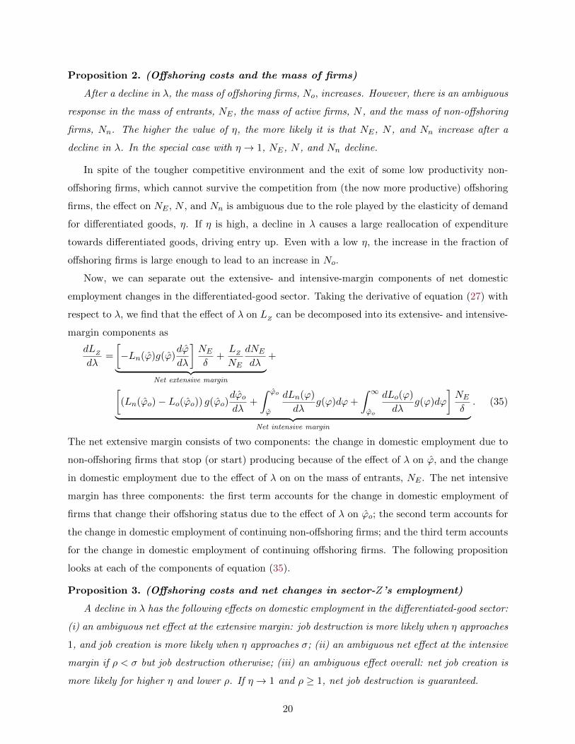
Let us now look at firm-level employment responses in the differentiated-good sector when λ
changes. Let L(ϕ) denote the demand for domestic labor of a firm with productivity ϕ so that
L(ϕ) = 0 if ϕ < ϕ, L(ϕ) = Ln(ϕ) if ϕ ∈ [ϕ, ϕo), and L(ϕ) = Lo(ϕ) if ϕ ≥ ϕo, where Ls(ϕ) is
15The theoretical results established earlier do not hinge on the assumption of a particular distribution. We usethe Pareto distribution for this numerical exercise because of its wide popularity in international trade models withheterogeneous firms, but similar results are obtained with other commonly used distributions.
22
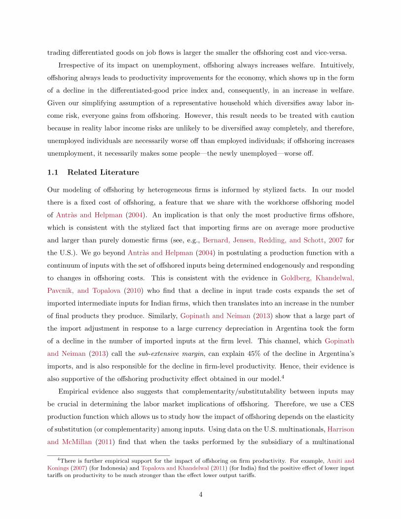
1 1.5 2.5 3 3.5 40
0.5
1
1.5
2
2.5
3
3.5
ϕ
λH
λLL(ϕ)
ϕϕ′ ϕoϕ′o
(a) Perfect input complementarity (ρ = 0)
1 2 2.5 3 40
0.5
1
1.5
2
2.5
3
3.5
ϕ
λH
λLL(ϕ)
ϕ ϕ′ ϕoϕ′o
(b) High input substitutability (ρ = 4 > σ)
Figure 1: Firm-level demand for domestic labor in differentiated-good sector: High offshoring cost(λ
H= 1.8) and low offshoring cost (λ
L= 1.2)
defined as in Lemma 3, for s ∈ n, o. Importantly, the elasticity of demand for Z, η, does not
affect firm-level labor outcomes because α, wZ , ϕ, and ϕo are independent of η, and therefore, L(ϕ)
is also independent of η.
Figure 1 shows L(ϕ) for a high offshoring cost (λH
= 1.8) and a low offshoring cost (λL
= 1.2)
under two cases: perfect input complementarity (ρ = 0) and high input substitutability (ρ = 4,
with ρ > σ). In both cases, the decline in λ causes an increase in the cutoff level that determines
whether or not a firm produces (from ϕ to ϕ′), and a decline in the cutoff level that separates
offshoring and non-offshoring firms (from ϕo to ϕ′o). Thus, each figure shows five types of firms
after a decline in λ: firms that never produce (ϕ < ϕ), non-offshoring firms that stop producing
(ϕ ≤ ϕ < ϕ′), non-offshoring firms that continue to produce (ϕ′ ≤ ϕ < ϕ′o), firms that begin to
offshore (ϕ′o ≤ ϕ < ϕo), and continuing offshoring firms (ϕ ≥ ϕo). From both figures, note that after
a decline in λ, we only observe job creation (though very small) for continuing offshoring firms in
the case of perfect input complementarity—for these firms, the productivity effect dominates both
the competition and job-relocation effects. For all other firms with ϕ ≥ ϕ, the decline in λ causes
job destruction: by death for firms with productivities between ϕ and ϕ′, and by contraction for
the rest of the firms.
The comparison of Figures 1a and 1b highlights one of the main results of this paper: the
crucial role of input complementarity/substitutability in determining the impact of offshoring on
domestic employment. Note that the negative impact of a decline in λ on firm-level employment
is much larger for the case of high input substitutability. To look further at this issue, Figure
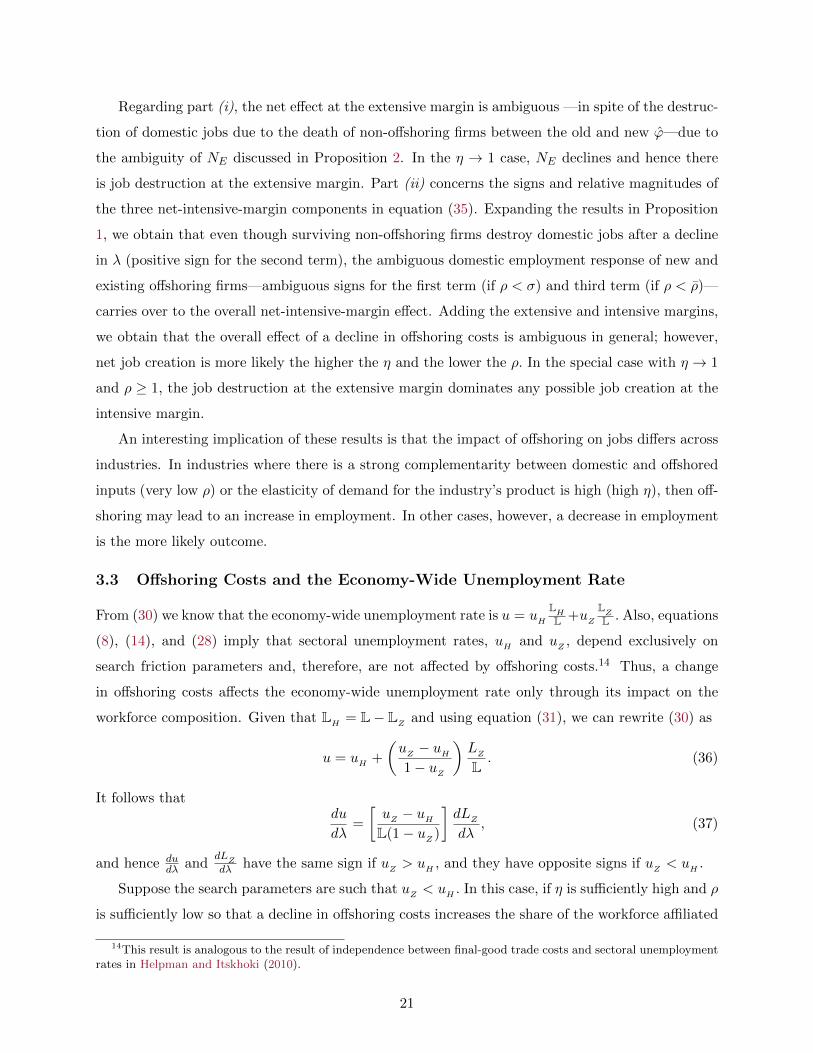
2 shows—from equation (27)—the relationship between λ and total domestic employment in the
23
1.1 1.2 1.3 1.4 1.5 1.6 1.7 1.8
0.3
0.4
0.5
0.6
0.7
0.8
0.9
ρL
ρM
ρH
LZ
λ
(a) Low elasticity of demand for Z (η = 1.5)
1.1 1.2 1.3 1.4 1.5 1.6 1.7 1.8
1.8
2.1
2.4
2.7
3ρL
ρM
ρH
LZ
λ
(b) High elasticity of demand for Z (η = 2.5)
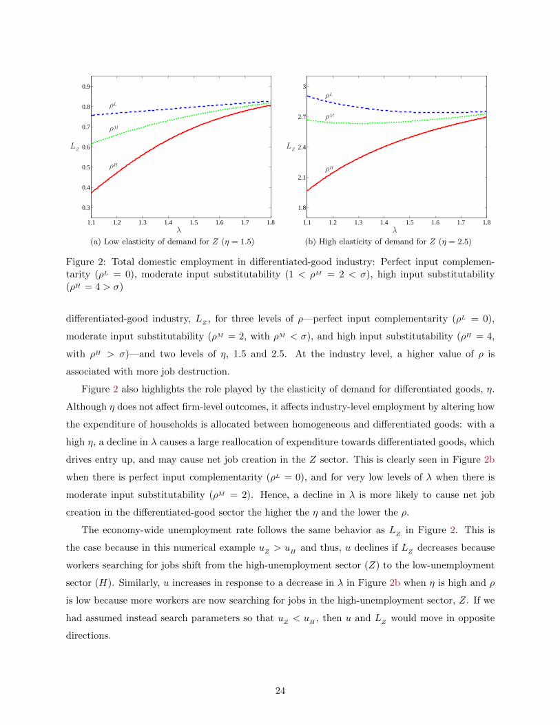
Figure 2: Total domestic employment in differentiated-good industry: Perfect input complemen-tarity (ρL = 0), moderate input substitutability (1 < ρM = 2 < σ), high input substitutability(ρH = 4 > σ)
differentiated-good industry, LZ , for three levels of ρ—perfect input complementarity (ρL = 0),
moderate input substitutability (ρM = 2, with ρM < σ), and high input substitutability (ρH = 4,
with ρH > σ)—and two levels of η, 1.5 and 2.5. At the industry level, a higher value of ρ is
associated with more job destruction.
Figure 2 also highlights the role played by the elasticity of demand for differentiated goods, η.
Although η does not affect firm-level outcomes, it affects industry-level employment by altering how
the expenditure of households is allocated between homogeneous and differentiated goods: with a
high η, a decline in λ causes a large reallocation of expenditure towards differentiated goods, which
drives entry up, and may cause net job creation in the Z sector. This is clearly seen in Figure 2b
when there is perfect input complementarity (ρL = 0), and for very low levels of λ when there is
moderate input substitutability (ρM = 2). Hence, a decline in λ is more likely to cause net job
creation in the differentiated-good sector the higher the η and the lower the ρ.
The economy-wide unemployment rate follows the same behavior as LZ in Figure 2. This is
the case because in this numerical example uZ > uH and thus, u declines if LZ decreases because
workers searching for jobs shift from the high-unemployment sector (Z) to the low-unemployment
sector (H). Similarly, u increases in response to a decrease in λ in Figure 2b when η is high and ρ
is low because more workers are now searching for jobs in the high-unemployment sector, Z. If we
had assumed instead search parameters so that uZ < uH , then u and LZ would move in opposite
directions.
24
3.5 Offshoring and Welfare
While the focus of our paper is on the employment effects of offshoring, we can also derive welfare
implications. Note from equation (3) that the welfare of the representative household is inversely
related to the price index, P, and positively related to the spending, E. From (6) and (33), it
follows that E does not change in response to a change in λ or fo. Since P declines in response to
either a decline in λ or fo (ϕ increases when λ or fo decline, and from (20) we know that P and ϕ
have an inverse relationship) we obtain the following result.
Proposition 4. (Offshoring and Welfare)
A decrease in the cost of offshoring (fixed or variable) leads to an increase in welfare.
Intuitively, offshoring always leads to productivity improvements for the economy, which shows
up in a lower price index for differentiated goods and consequently in an increase in welfare. The
result above is notable because we have labor market frictions in the model and it is possible
for a decrease in the cost of offshoring to lead to an increase in unemployment. As well, our
assumption of a representative household implies everyone gains from offshoring. As mentioned
in the Introduction, some caveats about this result are in order. First, in reality labor income
risk cannot be diversified away, which means that unemployed workers have lower welfare than
employed workers; an increase in unemployment induced by offshoring creates some losers—the
newly unemployed. Second, if workers are highly risk averse, any increase in unemployment caused
by offshoring can inflict large losses on workers by increasing the labor market risk, which then
must be weighed against the efficiency gains inherent in the proposition above. Since the focus
of this paper is on identifying the channels through which offshoring affects unemployment, we
abstract from these broader welfare issues by relying on the simplifying assumption of a risk neutral
representative household.
4 Search Frictions and Jobs
The impact of a change in search frictions can be easily studied in our model. The key equation
for this analysis is equation (15), which we recall is wZ ≡mH
mZ
(γZγH
)1−β. That is, search friction
parameters affect jobs by altering the cost of hiring a unit of domestic labor in the differentiated-
good sector, wZ . Given that β ∈ (0, 1), note that wZ is increasing in γZ and mH , and decreasing
in γH and mZ . There is a reduction in search frictions in sector i when either γi declines or mi
increases. Therefore, a reduction in search frictions in the differentiated-good sector lowers wZ ,
and a reduction in search frictions in the homogeneous-good sector increases wZ . The following
25
lemma contains results that will allow us to understand the effects of changes in search frictions on
offshoring decisions and jobs.
Lemma 5. ζα,wZ> 0, ζc(α),w
Z< 0, ζϕ,w
Z> 0, ζϕo,wZ < 0.
By lowering wZ , a decrease in search frictions in the differentiated-good sector makes offshoring
less attractive, which in turn reduces the fraction of offshored inputs, ζα,wZ> 0, and erodes the
relative cost advantage of offshoring firms, ζc(α),wZ< 0. The proportional decrease in the marginal
cost of offshoring firms is less than that of non-offshoring firms, which leads to a softening of the
competitive environment: ζϕ,wZ> 0. As well, the reduced attractiveness of offshoring leads to an
increase in the offshoring productivity cutoff: ζϕo,wZ < 0.
From (26) we obtain that the elasticity of firm-level domestic employment, Ls(ϕ), with respect
to wZ is given by
ζLs(ϕ),wZ
=
−(σ − 1)ζϕ,w
Z− 1 if s = n
− α1−αζα,wZ − (σ − ρ)ζc(α),w
Z− (σ − 1)ζϕ,w
Z− 1 if s = o.
(38)
After a decline in wZ , employment at non-offshoring firms increases not only because of the compe-
tition effect, −(σ− 1)ζϕ,wZ< 0, but also because of the direct effect of a decrease in their marginal
cost and the consequent increase in demand (accounted for by −1). For offshoring firms we again
have the three effects—job relocation, competition, and productivity—in addition to the direct
effect of a lower marginal cost. As before, the productivity effect moves in the opposite direction
to the other effects if ρ < σ, and in the same direction otherwise. Also ϕo increases, so there are
firms that stop offshoring—for these firms we observe the four effects directly from (26).
Proposition 5. (Search frictions and differentiated-good-sector employment)
A decline in search frictions in sector Z—or an increase in search frictions in sector H—
lowers wZ , which affects sector-Z’s domestic employment and the mass of firms as follows: (i) job
creation due to the birth of low productivity non-offshoring firms; (ii) job creation at continuing
non-offshoring firms; (iii) an ambiguous domestic labor response at continuing offshoring firms if
ρ < ρ, where ρ < σ− 1, but job creation otherwise; (iv) an ambiguous response at firms that switch
from offshoring to non-offshoring if ρ < σ, but job creation otherwise; (v) increases in NE, N ,
and Nn, but an ambiguous response in No; (vi) net job creation at the extensive margin, and an
ambiguous response at the intensive margin and overall if ρ < σ, but net job creation otherwise.
Finally, higher η and ρ promote stronger job creation when wZ declines.
One key difference from the case of a change in offshoring costs is that a change in search
frictions affects the economy-wide unemployment rate not only through its impact on the workforce
26
0.6 0.7 0.8 0.9 1 1.1 1.20
0.5
1
1.5
2
2.5
3
LZ
γZ
(a) Differentiated-good-sector domestic employment
0.6 0.7 0.8 0.9 1 1.1 1.2
4.3%
4.6%
4.9%
5.2%
5.5%
u
γZ
(b) Economy-wide unemployment rate
Figure 3: Search frictions in differentiated-good sector and unemployment
composition, but also through its effect on sectoral unemployment rates. For example, a decline
in γZ affects LZ via a decrease in wZ , but also causes a decline in uZ—see (14) and (28). From
(36) note that, as opposed to the simpler response for a change in λ in (37), the response of u to a
change in γZ is given by
du
dγZ=
1
(1− uZ )L
[(uZ − uH )
dLZdwZ
dwZdγZ
+
(1− uH1− uZ
)duZdγZ
LZ
]. (39)
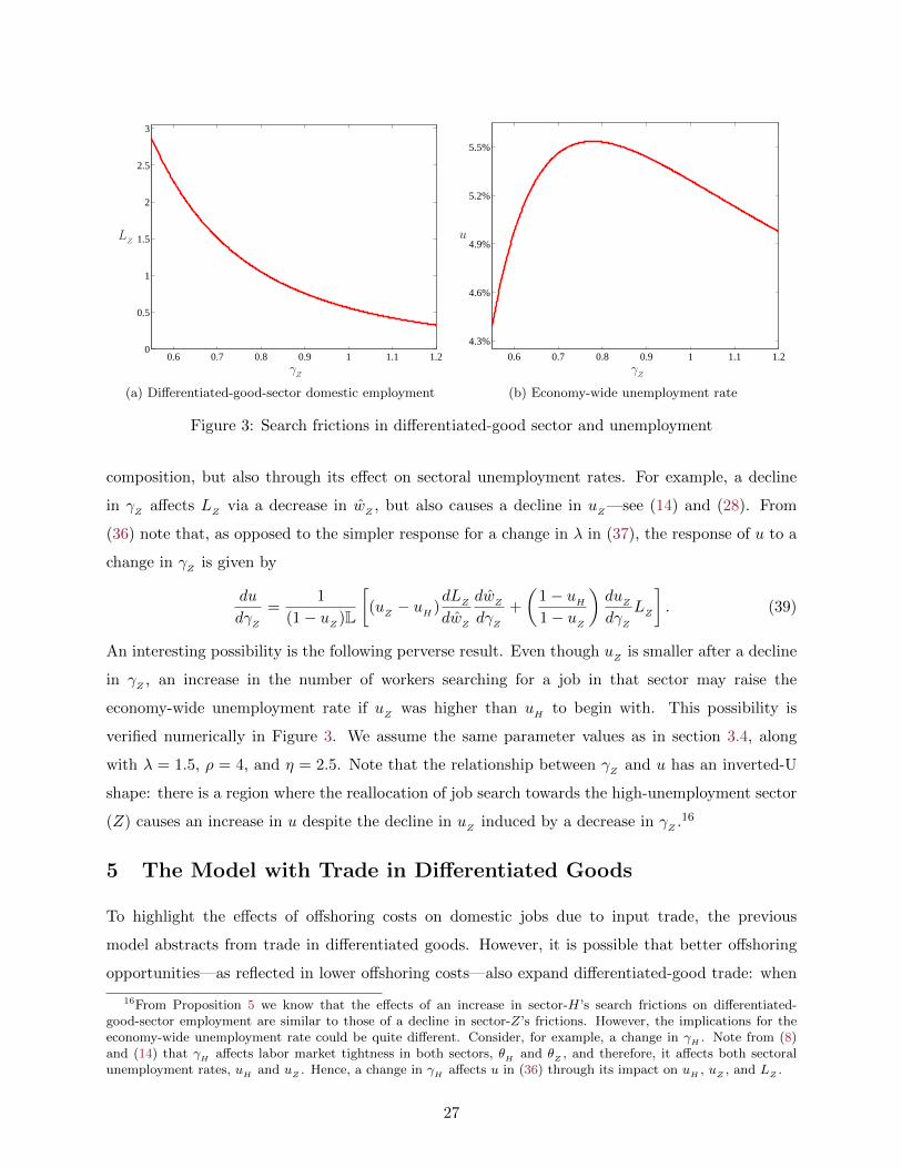
An interesting possibility is the following perverse result. Even though uZ is smaller after a decline
in γZ , an increase in the number of workers searching for a job in that sector may raise the
economy-wide unemployment rate if uZ was higher than uH to begin with. This possibility is
verified numerically in Figure 3. We assume the same parameter values as in section 3.4, along
with λ = 1.5, ρ = 4, and η = 2.5. Note that the relationship between γZ and u has an inverted-U
shape: there is a region where the reallocation of job search towards the high-unemployment sector
(Z) causes an increase in u despite the decline in uZ induced by a decrease in γZ .16
5 The Model with Trade in Differentiated Goods
To highlight the effects of offshoring costs on domestic jobs due to input trade, the previous
model abstracts from trade in differentiated goods. However, it is possible that better offshoring
opportunities—as reflected in lower offshoring costs—also expand differentiated-good trade: when
16From Proposition 5 we know that the effects of an increase in sector-H’s search frictions on differentiated-good-sector employment are similar to those of a decline in sector-Z’s frictions. However, the implications for theeconomy-wide unemployment rate could be quite different. Consider, for example, a change in γH . Note from (8)and (14) that γH affects labor market tightness in both sectors, θH and θZ , and therefore, it affects both sectoralunemployment rates, uH and uZ . Hence, a change in γH affects u in (36) through its impact on uH , uZ , and LZ .
27
a firm begins to offshore, it becomes more competitive in both domestic and foreign final-good mar-
kets. Hence, offshoring costs affect jobs through their impact on trade in differentiated goods as
well. To analyze these employment effects, this section introduces an explicit North-South version
of the model with trade in both intermediate inputs and final goods.
There are two countries, North and South, and two production sectors in each country: a
homogenous-good sector and a differentiated-good sector. The homogeneous good is traded cost-
lessly and is produced under perfect competition, while each variety of the differentiated good is
potentially tradable and is produced under monopolistic competition. Each country is inhabited
by a continuum of households in the unit interval. The number of workers in each household is L
in the North, and L∗ in the South. We denote the variables for the South with a star (*).
The description of preferences, demand, and the labor market for the North is similar to sections
2.1 and 2.2. Since our focus is on the North labor market, we abstract from any labor imperfections
in the South and assume it has a perfectly competitive labor market. One unit of Southern labor
produces w∗ < 1 units of the homogeneous good, and therefore, the wage in the South is w∗ as long
as some homogeneous good is produced there—which we assume to be the case. The preferences
of the representative household in the South are the same as in the North and hence, the South’s
market demand for variety ω is z∗c(ω) = p∗(ω)−σP ∗σ−η, where p∗(ω) is the Southern price of variety
ω and P ∗ is the South’s differentiated-good price index. The aggregate spending in the South is
simply E∗ = w∗L∗.
In both countries, producers in the differentiated-good sector are heterogeneous in productivity.
After drawing its productivity, each firm decides whether or not to produce for the domestic and
export markets. The decision to produce or not for a market is determined by the ability of the firm
to cover the fixed cost of selling in that market. Thus, in this extension there is two-way trade in
final differentiated goods. Moreover, costless trade in the homogeneous good ensures trade balance
between the two countries. As before, we assume that w∗ < wZ , so that the differentiated-good
producing firms in the North have an incentive to offshore input production to the South.
To keep the analysis tractable in the North-South extension, we make the simplifying assumption
that there are no fixed costs of offshoring (fo = 0), so that every producing firm in the North
offshores. This allows us to clearly isolate the channels through which variable offshoring costs
affect job flows and the economy-wide unemployment rate via their impact on trade in final goods.17
The production function of a Northern firm with productivity ϕ is defined as in section 2.3.1.
17In section B.4 in the Appendix we show the benchmark case with fo = 0. In this case, a decrease in λ benefits allfirms proportionately, and therefore, leaves ϕ—the minimum productivity level needed to cover the domestic-marketfixed costs—unaffected. However, the intensive-margin effects and the overall effect remain qualitatively similar.Figures B.1 and B.2 in the Appendix are plotted using the same parameters as in Figures 1 and 2, except that fo = 0.
28
The absence of fixed costs of offshoring implies that every active Northern firm offshores and hence
α(ϕ) = α for each of them. Equation (16) and Lemma 1 hold, and therefore, the marginal cost of
a Northern firm with productivity ϕ for selling in the Northern market isc(α)w
Zϕ . If the Northern
firm decides to export its finished good, its marginal cost for selling in the Southern market isτc(α)w
Zϕ , where τ > 1 accounts for an iceberg export cost—the Northern firm must ship τ units
of the good for one unit to reach the Southern market. Assuming market segmentation and given
CES preferences, the prices that a Northern firm with productivity ϕ sets in the domestic (D) and
export (X) markets are given by pD(ϕ) =(
σσ−1
)c(α)w
Zϕ and pX(ϕ) =
(σσ−1
)τc(α)w
Zϕ , respectively.
Using these pricing equations and the market demand functions, we obtain that this firm’s gross
profit functions—before deducting fixed costs—from selling in the domestic and export markets are
πD(ϕ) = 1σpD(ϕ)1−σP σ−η and πX(ϕ) = 1
σpX(ϕ)1−σP ∗σ−η, respectively.
Southern firms only use South labor. The production function for a Southern firm with pro-
ductivity ϕ is z∗(ϕ) = A∗ϕY ∗, where A∗ < 1 is an aggregate productivity factor for Southern
firms—they are less efficient than Northern firms in the production of differentiated goods—and
Y ∗ =(∫ 1
0 y∗(α)
ρ−1ρ dα
) ρρ−1
. With y∗(α) = `∗, and as L∗ = `∗, the production function is equiv-
alent to z∗(ϕ) = A∗ϕL∗. The marginal cost for this firm is then w∗
A∗ϕ from selling domestically,
and τw∗
A∗ϕ from selling in the Northern market. Therefore, the prices set by a Southern firm with
productivity ϕ are p∗D(ϕ) =(
σσ−1
)w∗
A∗ϕ in the domestic market, and p∗X(ϕ) =(
σσ−1
)τw∗
A∗ϕ in the
export market. This firm’s gross profit functions from selling in the domestic and export markets
are π∗D(ϕ) = 1σp∗D(ϕ)1−σP ∗σ−η and π∗X(ϕ) = 1
σp∗X(ϕ)1−σP σ−η, respectively.
5.1 Equilibrium in the North-South Model
There are fixed costs of selling in each market. These fixed costs along with the CES demand system
imply the existence of cutoff productivity levels that determine the tradability of each differentiated
good in each market. For Northern firms there are two cutoff productivity levels: one for selling in
the domestic market, ϕD, and one for selling in the South, ϕX .18 Similarly, ϕ∗D and ϕ∗X denote the
cutoff productivity levels for Southern firms.
As before, we assume that all fixed costs are in terms of the homogeneous good. For r ∈ D,X,let fr be the fixed cost of selling in market r for the Northern firms, and let f∗r be the fixed cost
of selling in market r for the Southern firms. Therefore, the cutoff productivity levels satisfy
πr(ϕr) = fr and π∗r (ϕ∗r) = f∗r , for r ∈ D,X. Thus, using the gross profit functions from the
18This version of the model assumes fo = 0 so that every producing Northern firm offshores. As in the benchmarkmodel, relaxing this assumption (i.e assuming instead fo > 0) implies the existence of a cutoff productivity level, ϕo,above which firms would offshore. Thus, Northern firms would be subject to three cutoff productivity levels: ϕD,ϕX , and ϕo. Depending on the differences between the fixed costs of production, offshoring, and exporting, we canhave various possible rankings of these cutoffs.
29
previous section, we obtain the following zero-cutoff-profit conditions:
pD(ϕD)1−σP σ−η = σfD, (40)
pX(ϕX)1−σP ∗σ−η = σfX , (41)
p∗D(ϕ∗D)1−σP ∗σ−η = σf∗D, (42)
p∗X(ϕ∗X)1−σP σ−η = σf∗X . (43)
Combining (40) and (43), and (41) and (42)—and using the pricing equations from the previous
section—we obtain
ϕ∗X =
(f∗XfD
) 1σ−1
[τw∗
A∗c(α)wZ
]ϕD, (44)
ϕX =
(fXf∗D
) 1σ−1
[τA∗c(α)wZ
w∗
]ϕ∗D. (45)
These equations indicate the link between the cutoff levels for firms selling in the same market.
Moreover, using the zero-cutoff-profit conditions (40)-(43), we can substitute out P and P ∗ in the
gross profit functions from the previous section to rewrite them as
πr(ϕ) =
(ϕ
ϕr
)σ−1
fr, (46)
π∗r (ϕ) =
(ϕ
ϕ∗r
)σ−1
f∗r , (47)
for r ∈ D,X.There is free entry of firms in both countries. Each entrant in either country must pay a sunk
entry cost in terms of the homogeneous good. The entry cost in the North is fE and the entry
cost in the South is f∗E . As a firm knows its productivity only after entry, the per-period pre-entry
expected profits for Northern and Southern potential entrants are, respectively, given by
Π ≡∫ ∞ϕD
[πD(ϕ)− fD] g(ϕ)dϕ+
∫ ∞ϕX
[πX(ϕ)− fX ] g(ϕ)dϕ, (48)
Π∗ ≡∫ ∞ϕ∗D
[π∗D(ϕ)− f∗D] g(ϕ)dϕ+
∫ ∞ϕ∗X
[π∗X(ϕ)− f∗X ] g(ϕ)dϕ, (49)
where the first term in Π and Π∗ represents the expected profits from selling domestically, and the
second term represents the expected profits from exporting. Given the exogenous death rate, δ, the
value of entry in the North is Πδ and the value of entry in the South is Π∗
δ . Therefore, the free-entry
conditions are
Π
δ= fE , (50)
Π∗
δ= f∗E . (51)
30
We can now define the equilibrium in the North-South model.
Definition 2. Given πr(ϕ), π∗r (ϕ), Π, and Π∗ in (46), (47), (48) and (49), an equilibrium is
a 6-tuple (wZ , α, ϕD, ϕX , ϕ∗D, ϕ
∗X) that solves (15), (16), (44), (45), (50), and (51). A sufficient
condition for the existence and uniqueness of equilibrium is that τ is sufficiently large so that
ϕD < ϕX and ϕ∗D < ϕ∗X .
As is usual in Melitz-type heterogeneous-firm models, we assume that the iceberg export cost
is large enough so that ϕD < ϕX and ϕ∗D < ϕ∗X : exporting firms always produce for the domestic
market. In section C.1 in the Appendix we show the existence and uniqueness of equilibrium under
this assumption.
Once we solve for the equilibrium, P and P ∗ are easily determined from (40) and (41). We can
also solve for the number of firms selling in each market. Let N and N∗ denote, respectively, the
masses of sellers of differentiated goods in the North and South. In the North, N is composed of a
mass of ND Northern firms and a mass of N∗X Southern firms, so that N = ND + N∗X . Similarly,
N∗ = N∗D +NX , where N∗D is the mass of Southern producers selling domestically, and NX is the
mass of Northern exporters. In steady state, the firms that die due to the exogenous death shock are
exactly replaced by successful entrants so that δNr = [1−G(ϕr)]NE and δN∗r = [1−G(ϕ∗r)]N∗E ,
where NE and N∗E denote the masses of Northern and Southern entrants every period, G(ϕ) is the
cumulative distribution function from which Northern and Southern firms draw their productivities
after entry, and r ∈ D,X. Thus, to obtain expressions for ND, NX , N∗D, and N∗X in terms of
wZ , α, and the cutoff levels, we need to derive first the expressions for NE and N∗E . Section C.2 in
the Appendix derives NE and N∗E .
5.2 Employment
Employment in the differentiated-good sector in the North is determined as follows. Recall that
with fo = 0, every producing Northern firm offshores. Hence, Northern firms demand Southern
labor for inputs in the range [0, α], and demand Northern labor for inputs in the range [α, 1]. Let
Lr(ϕ) denote the demand for domestic labor of a Northern firm with productivity ϕ to produce for
market r, where r ∈ D,X. The following lemma presents Lr(ϕ).
Lemma 6. The amount of Northern labor required by a Northern firm with productivity ϕ to
produce for market r is given by
Lr(ϕ) =(1− α)(σ − 1)
c(α)1−ρwZ
(ϕ
ϕr
)σ−1
fr if ϕ ≥ ϕr, (52)
and zero otherwise, for r ∈ D,X.
31
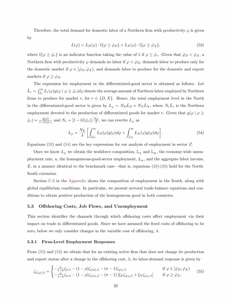
Therefore, the total demand for domestic labor of a Northern firm with productivity ϕ is given
by
L(ϕ) = LD(ϕ) · Iϕ ≥ ϕD+ LX(ϕ) · Iϕ ≥ ϕX, (53)
where Iϕ ≥ ϕr is an indicator function taking the value of 1 if ϕ ≥ ϕr. Given that ϕD < ϕX , a
Northern firm with productivity ϕ demands no labor if ϕ < ϕD, demands labor to produce only for
the domestic market if ϕ ∈ [ϕD, ϕX), and demands labor to produce for the domestic and export
markets if ϕ ≥ ϕX .
The expression for employment in the differentiated-good sector is obtained as follows. Let
Lr =∫∞ϕrLr(ϕ)g(ϕ | ϕ ≥ ϕr)dϕ denote the average amount of Northern labor employed by Northern
firms to produce for market r, for r ∈ D,X. Hence, the total employment level in the North
in the differentiated-good sector is given by LZ = NDLD + NX LX , where NrLr is the Northern
employment devoted to the production of differentiated goods for market r. Given that g(ϕ | ϕ ≥ϕr) = g(ϕ)
1−G(ϕr)and Nr = [1−G(ϕr)]
NEδ , we can rewrite LZ as
LZ =NE
δ
[∫ ∞ϕD
LD(ϕ)g(ϕ)dϕ+
∫ ∞ϕX
LX(ϕ)g(ϕ)dϕ
]. (54)
Equations (52) and (54) are the key expressions for our analysis of employment in sector Z.
Once we know LZ we obtain the workforce composition, LZ and LH , the economy-wide unem-
ployment rate, u, the homogeneous-good-sector employment, LH , and the aggregate labor income,
E, in a manner identical to the benchmark case—that is, equations (28)-(33) hold for the North-
South extension.
Section C.3 in the Appendix shows the composition of employment in the South, along with
global equilibrium conditions. In particular, we present sectoral trade-balance equations and con-
ditions to obtain positive production of the homogeneous good in both countries.
5.3 Offshoring Costs, Job Flows, and Unemployment
This section identifies the channels through which offshoring costs affect employment via their
impact on trade in differentiated goods. Since we have assumed the fixed costs of offshoring to be
zero, below we only consider changes in the variable cost of offshoring, λ.
5.3.1 Firm-Level Employment Responses
From (52) and (53) we obtain that for an existing active firm that does not change its production
and export status after a change in the offshoring cost, λ, its labor-demand response is given by
ζL(ϕ),λ =
− α
1−αζα,λ − (1− ρ)ζc(α),λ − (σ − 1)ζϕD,λ if ϕ ∈ [ϕD, ϕX)
− α1−αζα,λ − (1− ρ)ζc(α),λ − (σ − 1) [ξDζϕD,λ + ξXζϕX ,λ] if ϕ ≥ ϕX ,
(55)
32
where each ζ · ,λ represents an elasticity with respect to λ, ξD = LD(ϕ)L(ϕ) , and ξX = 1 − ξD.19 The
following lemma shows the signs of the elasticities in the right-hand side of equation (55).
Lemma 7. ζα,λ < 0, ζc(α),λ > 0, ζϕD,λ < 0, ζϕX ,λ > 0.
The elasticities ζα,λ and ζc(α),λ are identical to those obtained in the benchmark case, and
as before, they give rise to the job-relocation and productivity effects. Note, however, that the
coefficient of ζc(α),λ in (55) is −(1−ρ) rather than −(σ−ρ) as was the case in equation (34) for the
benchmark model. The difference arises because the productivity effect for offshoring firms in the
benchmark case has two components: an absolute productivity effect and a relative productivity
effect. The latter arises from the fact that the productivity of these firms—and consequently their
market share—increases relative to the productivity of non-offshoring firms. Since all firms offshore
in the North-South extension, only the absolute productivity effects is present, and therefore,
complementarity between inputs (ρ < 1) is both necessary and sufficient for the productivity effect
to be a source of job creation.
Additionally, we have competition effects in both the domestic and export markets—these effects
are driven, respectively, by ζϕD,λ and ζϕX ,λ. Note that after a fall in λ, the competitive environment
becomes tougher in the North, ζϕD,λ < 0: as profit opportunities for Northern firms increase due
to the decline in λ—Northern firms become more competitive relative to Southern firms—entry
expands in the North to the point that the free-entry condition is satisfied again. This reduces the
residual domestic demand for all Northern firms, and hence, ϕD (the productivity that is needed to
exactly meet fD) increases. After a decline in λ, the domestic-market competition effect is a source
of job losses for both exporting and non-exporting firms. On the other hand, entry of Southern
firms decreases—their profit opportunities decline and hence entry must decrease to satisfy the
free-entry condition—and therefore, Northern firms face an easier competitive environment in the
South. This is reflected in a lower ϕX (ζϕX ,λ > 0) and a higher residual demand for the good of each
Northern exporter. This is the new effect introduced by our extension with trade in differentiated
goods. We label it “export-market competition effect” and after a decline in λ, is a source of job
creation for exporting firms.
From (55) note that non-exporting firms experience the same three effects as offshoring firms
in the benchmark case: job-relocation, productivity, and (domestic-market) competition effects.20
19ξD =fD/(ϕ
σ−1D
)
fD/(ϕσ−1D
)+fX/(ϕσ−1X
), which is the same for every ϕ ≥ ϕX .
20If we assume fo > 0 (so that an offshoring cutoff productivity level, ϕo, exists) and if the fixed costs are suchthat ϕD < ϕo < ϕX—so that the most productive firms do both exporting and offshoring while the least productivefirms do neither—then a decrease in λ will have an unambiguous adverse effect on jobs in the non-offshoring Northernfirms (those firms with productivities between ϕD and ϕo), a result that was present in the benchmark case. Otherthan that, the qualitative results of the North-South model remain unchanged, and therefore, we use the fo = 0assumption in the interest of clarity and to focus on the new effects arising due to exporting possibilities.
33
In addition to these three effects, exporting firms experience the export-market competition effect.
The following proposition describes the net effects of a change in the offshoring cost on these firms’
employment, along with the net effects on firms that change their production or export status.
Proposition 6. (Offshoring costs and Northern firm-level employment)
In the North’s differentiated-good sector, a decline in λ leads to: (i) the death of the least
productive non-exporting firms, who then destroy all their jobs; (ii) an ambiguous domestic labor
response at surviving non-exporting firms if ρ < ρ, where ρ < 1, but job destruction otherwise; (iii)
an ambiguous domestic labor response at existing exporting firms if ρ < ρ, where ρ ∈ (1, σ), but
job destruction otherwise; (iv) an ambiguous domestic labor response at existing firms that start
exporting.
Part (i) follows from the result that ϕD increases in response to a decline in λ. Regarding
part (ii), recall that for active non-exporting firms, the only source of job creation after a decline
in λ is the productivity effect when ρ < 1—input complementarity is necessary but not sufficient
for job creation in these firms. As for part (iii), we know that continuing exporting firms have
also the export-market competition effect as a source of job creation. This effect dominates the
domestic-market competition effect and hence, these firms may create jobs even if ρ > 1 : input
complementarity is neither necessary nor sufficient for job creation in continuing exporting firms
after a decline in λ. Concerning part (iv), note that as ϕX declines some active Northern firms
change their status from non-exporting to exporting. From (53) we can see that these firms have
a discrete jump in their labor-demand function as they begin to export. These firms may create
jobs after a decline in λ, even if ρ > σ, because of the job creating force of the export-market
competition effect.
We perform a numerical exercise to illustrate our main results. We use the same assumptions
and parameter values as in section 3.4, with the exception of the value for fo, which is zero in
the North-South extension. We also have additional parameters. The total size of the workforce
in the South, L∗, is set at 15 (identical to the North). As in the North, the sunk entry cost in
the South is f∗E = 0.8. The fixed costs of operating domestically and the fixed costs of exporting
are identical across countries, fD = f∗D = fX = f∗X = 0.05. We set the aggregate productivity
parameter for Southern differentiated-good firms, A∗, to 0.48. Lastly, we set the iceberg cost for
trade in differentiated goods, τ , at 1.7.
Figure 4 presents L(ϕ), given in (53), for a high offshoring cost (λH
= 1.8) and a low offshoring
cost (λL
= 1.2) for the cases of perfect input complementarity (ρ = 0) and high input substitutabil-
ity (ρ = 4 > σ). Consistent with the first part of Proposition 6, after a decline in λ Figures 4a
and 4b show job destruction by death for firms with productivities between ϕD and ϕ′D. For firms
34
1 1.2 1.4 1.6 20
0.1
0.2
0.3
0.4
0.5
0.6
ϕ
λH
λL
L(ϕ)
ϕDϕ′
Dϕ
Xϕ′
X
(a) Perfect input complementarity (ρ = 0)
1 1.4 1.8 20
0.1
0.2
0.3
0.4
0.5
0.6
ϕ
λH
λLL(ϕ)
ϕDϕ′
Dϕ
Xϕ′
X
(b) High input substitutability (ρ = 4 > σ)
Figure 4: Firm-level demand for Northern labor in sector Z: High offshoring cost (λH
= 1.8) and
low offshoring cost (λL
= 1.2)
with ϕ ≥ ϕ′D, Proposition 6 says that the impact of a decline in offshoring costs on employment
is ambiguous. In the case of perfect input complementarity (Figure 4a), our numerical example
shows job creation for firms that begin to export (ϕ ∈ [ϕ′X , ϕX)), and job destruction in the other
cases. However, with ρ = 0, the decline in employment is small for both continuing non-exporting
firms (ϕ ∈ [ϕ′D, ϕ′X)) and continuing exporting firms (ϕ ≥ ϕX). On the other hand, Figure 4b
shows that for a high elasticity of substitution between inputs, a decrease in λ causes a decline in
employment for all firms; however, the decline is smaller (in proportion to previous employment)
for firms that begin to export.21 As in Figure 1, Figures 4a and 4b show the importance of ρ in
determining the impact of offshoring on firm-level employment.
5.3.2 Industry-Level Employment Responses
Changes in offshoring costs affect the number of firms in the economy, and hence there are also
changes at the extensive margin of employment. The following proposition looks into the responses
of the different masses of Northern firms when λ changes.
Proposition 7. (Offshoring costs, differentiated-good trade, and the masses of firms)
For Northern firms, a decline in the offshoring cost, λ, causes: (i) increases in the mass of
entrants (NE) and the mass of exporting firms (NX); (ii) an ambiguous effect on the mass of firms
21In the comparison of Figures 1a and 4a, note that while a decline in offshoring costs leads to net job creationfor the most productive firms in Figure 1a, it leads to net job destruction for the most productive firms in Figure 4a.Recall, however, that Figure 1a was constructed using fo = 0.05, while we use fo = 0 in the construction of Figure4a. For the model without differentiated-good trade with fo = 0, Figure B.1 in the Appendix shows that a decreasein offshoring costs leads to small job losses even for high productivity firms.
35
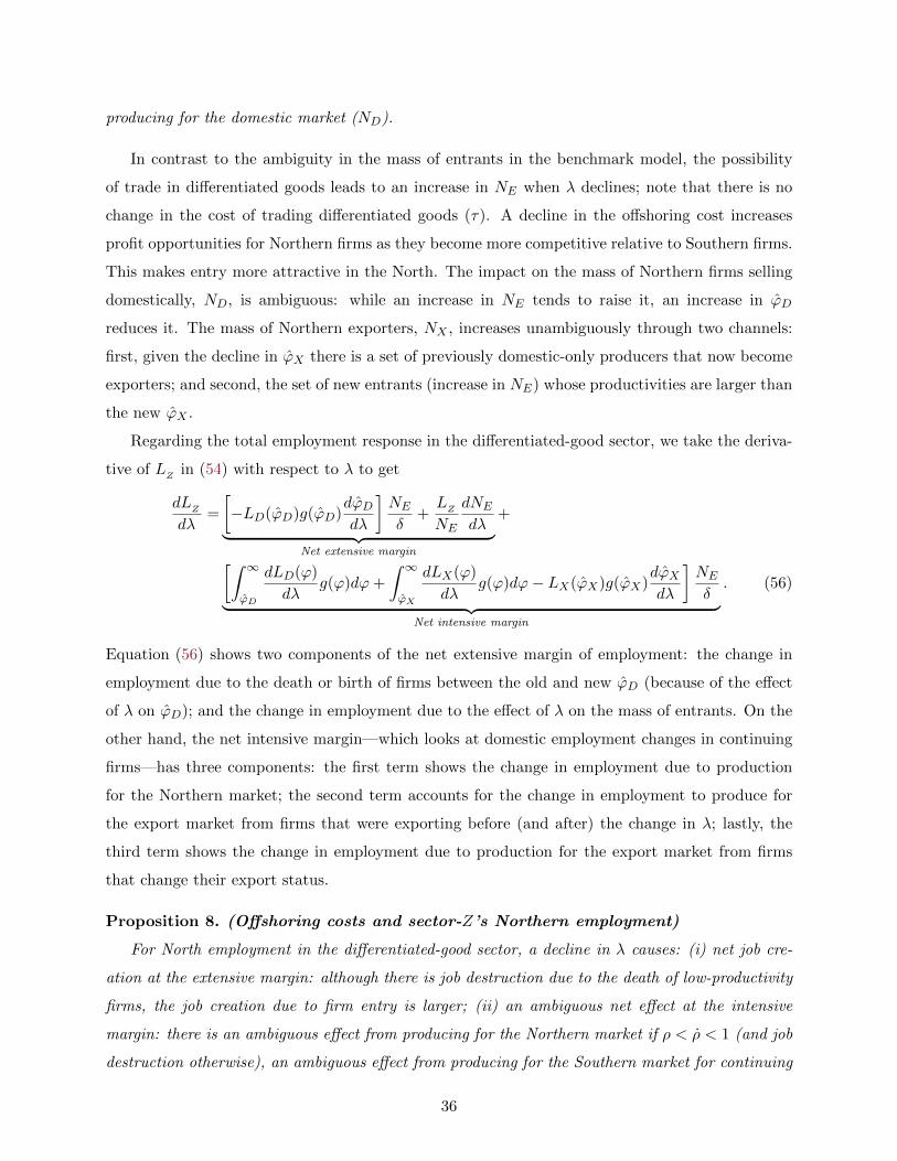
producing for the domestic market (ND).
In contrast to the ambiguity in the mass of entrants in the benchmark model, the possibility
of trade in differentiated goods leads to an increase in NE when λ declines; note that there is no
change in the cost of trading differentiated goods (τ). A decline in the offshoring cost increases
profit opportunities for Northern firms as they become more competitive relative to Southern firms.
This makes entry more attractive in the North. The impact on the mass of Northern firms selling
domestically, ND, is ambiguous: while an increase in NE tends to raise it, an increase in ϕD
reduces it. The mass of Northern exporters, NX , increases unambiguously through two channels:
first, given the decline in ϕX there is a set of previously domestic-only producers that now become
exporters; and second, the set of new entrants (increase in NE) whose productivities are larger than
the new ϕX .
Regarding the total employment response in the differentiated-good sector, we take the deriva-
tive of LZ in (54) with respect to λ to get
dLZdλ
=
[−LD(ϕD)g(ϕD)
dϕDdλ
]NE
δ+LZNE
dNE
dλ︸ ︷︷ ︸Net extensive margin
+
[∫ ∞ϕD
dLD(ϕ)
dλg(ϕ)dϕ+
∫ ∞ϕX
dLX(ϕ)
dλg(ϕ)dϕ− LX(ϕX)g(ϕX)
dϕXdλ
]NE
δ︸ ︷︷ ︸Net intensive margin
. (56)
Equation (56) shows two components of the net extensive margin of employment: the change in
employment due to the death or birth of firms between the old and new ϕD (because of the effect
of λ on ϕD); and the change in employment due to the effect of λ on the mass of entrants. On the
other hand, the net intensive margin—which looks at domestic employment changes in continuing
firms—has three components: the first term shows the change in employment due to production
for the Northern market; the second term accounts for the change in employment to produce for
the export market from firms that were exporting before (and after) the change in λ; lastly, the
third term shows the change in employment due to production for the export market from firms
that change their export status.
Proposition 8. (Offshoring costs and sector-Z’s Northern employment)
For North employment in the differentiated-good sector, a decline in λ causes: (i) net job cre-
ation at the extensive margin: although there is job destruction due to the death of low-productivity
firms, the job creation due to firm entry is larger; (ii) an ambiguous net effect at the intensive
margin: there is an ambiguous effect from producing for the Northern market if ρ < ρ < 1 (and job
destruction otherwise), an ambiguous effect from producing for the Southern market for continuing
36
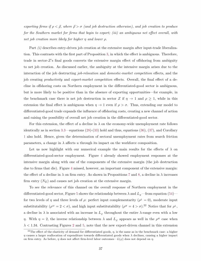
exporting firms if ρ < ~ρ, where ~ρ > σ (and job destruction otherwise), and job creation to produce
for the Southern market for firms that begin to export; (iii) an ambiguous net effect overall, with
net job creation more likely for higher η and lower ρ.
Part (i) describes entry-driven job creation at the extensive margin after input-trade liberaliza-
tion. This contrasts with the first part of Proposition 3, in which the effect is ambiguous. Therefore,
trade in sector-Z’s final goods converts the extensive margin effect of offshoring from ambiguity
to net job creation. As discussed earlier, the ambiguity at the intensive margin arises due to the
interaction of the job destructing job-relocation and domestic-market competition effects, and the
job creating productivity and export-market competition effects. Overall, the final effect of a de-
cline in offshoring costs on Northern employment in the differentiated-good sector is ambiguous,
but is more likely to be positive than in the absence of exporting opportunities—for example, in
the benchmark case there is net job destruction in sector Z if η → 1 and ρ ≥ 1, while in this
extension the final effect is ambiguous when η → 1 even if ρ > σ. Thus, extending our model to
differentiated-good trade expands the influence of offshoring costs, creating a new channel of action
and raising the possibility of overall net job creation in the differentiated-good sector.
For this extension, the effect of a decline in λ on the economy-wide unemployment rate follows
identically as in section 3.3—equations (28)-(33) hold and thus, equations (36), (37), and Corollary
1 also hold. Hence, given the determination of sectoral unemployment rates from search friction
parameters, a change in λ affects u through its impact on the workforce composition.
Let us now highlight with our numerical example the main results for the effects of λ on
differentiated-good-sector employment. Figure 4 already showed employment responses at the
intensive margin along with one of the components of the extensive margin (the job destruction
due to firms that die). Figure 4 missed, however, an important component of the extensive margin:
the effect of a decline in λ on firm entry. As shown in Propositions 7 and 8, a decline in λ increases
firm entry (NE) and causes net job creation at the extensive margin.
To see the relevance of this channel on the overall response of Northern employment in the
differentiated-good sector, Figure 5 shows the relationship between λ and LZ—from equation (54)—
for two levels of η and three levels of ρ: perfect input complementarity (ρL = 0), moderate input
substitutability (ρM = 2 < σ), and high input substitutability (ρH = 4 > σ).22 Notice that for ρL ,
a decline in λ is associated with an increase in LZ throughout the entire λ-range even with a low
η. With η = 2, the inverse relationship between λ and LZ appears as well in the ρH case when
λ < 1.34. Contrasting Figures 2 and 5, note that the new export-driven channel in this extension
22The effect of the elasticity of demand for differentiated goods, η, is the same as in the benchmark case: a higherη causes a larger reallocation of expenditure towards differentiated goods when λ declines, causing a higher impacton firm entry. As before, η does not affect firm-level labor outcomes—L(ϕ) does not depend on η.
37
1.1 1.2 1.3 1.4 1.5 1.6 1.7 1.8
0.5
0.6
0.7
0.8
0.9
ρL
ρM
ρH
LZ
λ
(a) η = 1.5
1.1 1.2 1.3 1.4 1.5 1.6 1.7 1.8
1.1
1.2
1.3
1.4
1.5
1.6
ρL
ρM
ρH
LZ
λ
(b) η = 2
Figure 5: Northern employment in sector Z and offshoring costs: Perfect input complementarity(ρL = 0), moderate input substitutability (ρM = 2 < σ), high input substitutability (ρH = 4 > σ)
makes net job creation in sector Z more likely.
5.4 Trade Liberalization in Differentiated Goods
As mentioned earlier, our two-sector structure is similar to Helpman and Itskhoki (2010), except
for the differences in (i) the wage-setting approach in the labor market, and (ii) the production
function of differentiated-good firms, which in our case allows us to analyze the implications of
offshoring. As to the consequences of final-good trade liberalization—which is the only type of
trade liberalization that Helpman-Itskhoki consider—the results of our model are the same as
in their asymmetric-countries case.23 The following lemma shows the signs for the relationship
between the cost of trading differentiated goods, τ , and the cutoff productivity levels.
Lemma 8. ζϕD,τ < 0, ζϕX ,τ > 0, ζϕ∗D,τ < 0, ζϕ∗X ,τ > 0.
Hence, as pointed out by Melitz (2003), a decline in the cost of trading differentiated goods
leads to an increase in the domestic productivity cutoff and a decrease in the exporting cutoff in
both countries. Given that τ does not affect wZ , α, or c(α), the impact on firm-level Northern
employment in sector Z can be easily derived from (52) and (53) as follows:
ζL(ϕ),τ =
−(σ − 1)ζϕD,τ if ϕ ∈ [ϕD, ϕX)
−(σ − 1) [ξDζϕD,λ + ξXζϕX ,λ] if ϕ ≥ ϕX .(57)
23While asymmetry in the Helpman-Itskhoki setup arises due to differences in labor market frictions across coun-tries, in our setup there is no labor market frictions in the South. Nevertheless, labor market frictions in the Northare sufficient to generate differences in the costs of producing differentiated goods across countries and therefore, ourresults with respect to changes in τ described below are very similar to those in Helpman and Itskhoki (2010).
38
It follows from Lemma 8 that non-exporting firms shed jobs—the least productive of them die while
the rest destroy jobs by contraction. Continuing exporting firms experience two opposing effects:
they experience a contraction from selling to the home market, and an expansion from selling to
the foreign market. Also, since ϕX declines, some previously purely-domestic firms start exporting.
These firms experience a discrete jump in labor requirements to meet export sales. It is worth
contrasting the effects of a decline in τ (final-good trade liberalization) with those of a decline in
λ (input trade liberalization): the job-relocation and productivity effects are only present in the
latter case.
The impact on overall employment in the differentiated-good sector is given bydL
Zdτ , whose
expression is similar to (56) with dλ replaced by dτ . As in the Helpman-Itskhoki model, τ does not
affect sectoral unemployment rates and therefore, the response of the economy-wide unemployment
rate, dudτ , is analogous to (37) with dλ replaced by dτ : similar to the effect of λ, τ affects the
unemployment rate only through its impact on the workforce composition,LZL and
LHL .
As was also the case in Helpman and Itskhoki (2010), it is difficult to derive analytical results for
economy-wide unemployment in the case of two asymmetric countries. We can, however, provide
intuitive results that we confirm with numerical illustrations. If the North has a comparative
advantage in the differentiated-good sector, then a decline in τ increases both LZ and the share
of the workforce going to the differentiated-good sector in the North. If labor market frictions
are higher in the differentiated-good sector so that uZ > uH , then a reduction in τ also leads
to an increase in unemployment in the North. Therefore, the effect of τ on the economy-wide
unemployment rate depends on two factors: (ii) whether the North has a comparative advantage in
the differentiated-good sector; and (ii) whether the search frictions are higher in the differentiated-
good sector or the homogeneous-good sector. In contrast, the results in the previous sections for
a change in offshoring costs obtain irrespective of whether the North has a comparative advantage
in the differentiated-good sector as long as the equilibrium is one with incomplete specialization.
Continuing with our numerical example, Figure 6 shows the relationship between τ and LZ for
two levels of offshoring costs (λH
= 1.8, λL
= 1.2), two levels of η (1.5 and 2), and ρ = 2. In this
example the North has a comparative advantage in producing differentiated goods and therefore, it
shows an inverse relationship between τ and LZ .24 Figure 6 also highlights the strong interaction
between input trade liberalization and final-good trade liberalization. Note that the effect of final-
good trade liberalization on LZ crucially depends on the extent of input trade liberalization: the
24We choose the value of A∗ so that the North is always—throughout our assumed range for λ—a net exporterof differentiated goods. Importantly (and realistically), even if the North is a net exporter of (final) differentiatedgoods, the North may still run a deficit in its sector-Z’s trade balance. This may be the case because sector Z in theNorth is a net importer of inputs (due to offshoring), and the value of these net imports may well be larger than thevalue of its net exports of final goods.
39
1.3 1.4 1.5 1.6 1.7 1.8 1.9 2 2.1
0.7
0.8
0.9
1λL
λH
LZ
τ
(a) η = 1.5
1.3 1.4 1.5 1.6 1.7 1.8 1.9 2 2.1
1.2
1.4
1.6
1.8
2 λL
λH
LZ
τ
(b) η = 2
Figure 6: Northern employment and final-good trade costs in sector Z: High offshoring cost (λH
=
1.8) and low offshoring cost (λL
= 1.2)
impact of a reduction in τ on differentiated-good-sector employment is larger the lower the λ.
Figure 6a also shows that input trade liberalization and final-good trade liberalization can have
opposite effects on LZ , and hence different labor market implications. Note that when η = 1.5 and
τ is high (e.g. τ = 2), the decline in offshoring costs from λH
to λL
causes net job destruction
in the differentiated-good sector. On the other hand, for both values of λ a reduction in τ causes
net job creation in the differentiated good sector. This implies that input trade liberalization and
final-good trade liberalization can have opposite effects on the economy-wide unemployment rate.
Figure 7 highlights this point by showing the relationship between u and λ, and u and τ , for the
cases of perfect input complementarity and high input substitutability. In this numerical example
uZ > uH—labor market frictions are higher in sector Z—and thus, LZ and u move in the same
direction when either λ or τ changes. Note that in the ρH
case, input trade liberalization (a decline
in λ) causes a decrease in the economy-wide unemployment rate because workers searching for jobs
move from the high-unemployment sector (Z) to the low-unemployment sector (H); the opposite
happens with final-good trade liberalization (a decline in τ). With perfect input complementarity,
both types of liberalization increase the economy-wide unemployment rate. Hence, input trade
liberalization is more likely to have the opposite effect on the economy-wide unemployment rate
than final-good trade liberalization for lower η and higher ρ.
Lastly, we can also do comparative statics with respect to the parameters governing search
frictions in the North-South extension. The results are similar to those derived in the benchmark
model except for the addition of the export competition effect. We present those results in section
40
1.1 1.2 1.3 1.4 1.5 1.6 1.7 1.8
4.03%
4.06%
4.09%
4.12%
4.15%
4.18%ρL
ρH
u
λ
(a) Changes in offshoring cost
1.3 1.4 1.5 1.6 1.7 1.8 1.9 2 2.1
4.06%
4.09%
4.12%
4.15%
4.18%
4.21%
4.24%
ρL
ρH
u
τ
(b) Changes in differentiated-good trade cost
Figure 7: Unemployment rates can move in opposite directions (η = 1.5): Perfect input comple-mentarity (ρL = 0) and high input substitutability (ρH = 4 > σ)
C.4 in the Appendix.
6 Conclusions
We constructed a two-sector theoretical model with labor market frictions to study the impact of
offshoring on job flows at the firm and industry levels and on the economy-wide unemployment rate.
We identify three channels through which a reduction in the cost of offshoring affects intrafirm and
intrasectoral reallocation in the differentiated-good sector: a job-relocation effect, a productivity
effect, and a competition effect. After a decline in offshoring costs, the job-relocation and com-
petition effects generate job losses, while the productivity effect can generate job expansions for
offshoring firms. The key parameters determining the impact of offshoring on reallocation of jobs
at various margins as well as on the economy-wide unemployment are the elasticity of substitution
between inputs and the elasticity of demand for differentiated goods.
Allowing differentiated-good producing firms to export creates an additional channel through
which a reduction in the cost of offshoring affects jobs and unemployment. Since offshoring lowers
the marginal cost of production, firms gain a competitive advantage in the export market, leading to
more job creation at both the intensive and the extensive margins. The implications of a reduction
in the cost of trading differentiated goods for job flows and unemployment can be very different
from those of a reduction in the offshoring cost. As well, the two trading costs interact in significant
ways. The impact of a decrease in the cost of trading differentiated goods on job flows is larger the
smaller the offshoring cost.
41
References
Amiti, M., and J. Konings (2007): “Trade Liberalization, Intermediate Inputs, and Productivity:
Evidence from Indonesia,” American Economic Review, 97(5), 1611–1638.
Amiti, M., and S.-J. Wei (2005): “Fear of Service Outsourcing: Is It Justified?,” Economic
Policy, 20(42), 308–347.
(2009): “Service Offshoring and Productivity: Evidence from the US,” The World Econ-
omy, 32(2), 203–220.
Antras, P., and E. Helpman (2004): “Global Sourcing,” Journal of Political Economy, 112(3),
552–580.
Bernard, A. B., J. B. Jensen, S. J. Redding, and P. K. Schott (2007): “Firms in Interna-
tional Trade,” Journal of Economic Perspectives, 21(3), 105–130.
Bernard, A. B., J. B. Jensen, and P. K. Schott (2009): “Importers, Exporters and Multi-
nationals: A Portrait of Firms in the U.S. that Trade Goods,” in Producer Dynamics: New
Evidence from Micro Data, pp. 513–552. University of Chicago Press.
Bernard, A. B., S. J. Redding, and P. K. Schott (2007): “Comparative Advantage and
Heterogeneous Firms,” Review of Economic Studies, 74(1), 31–66.
Biscourp, P., and F. Kramarz (2007): “Employment, Skill Structure and International Trade:
Firm-Level Evidence for France,” Journal of International Economics, 72(1), 22–51.
Davidson, C., and S. J. Matusz (2004): International Trade and Labor Markets: Theory,
Evidence, and Policy Implications. W. E. Upjohn Institute.
(2005): “Trade and Turnover: Theory and Evidence,” Review of International Economics,
13(5), 861–880.
Davidson, C., S. J. Matusz, and A. Shevchenko (2008): “Outsourcing Peter To Pay Paul:
High-Skill Expectations And Low-Skill Wages With Imperfect Labor Markets,” Macroeconomic
Dynamics, 12(4), 463–479.
Egger, H., U. Kreickemeier, and J. Wrona (2013): “Offshoring Domestic Jobs,” CESifo
Working Paper Series 4083, CESifo Group Munich.
Felbermayr, G., J. Prat, and H.-J. Schmerer (2011): “Globalization and labor market out-
comes: Wage bargaining, search frictions, and firm heterogeneity,” Journal of Economic Theory,
146(1), 39–73.
Goldberg, P. K., A. K. Khandelwal, N. Pavcnik, and P. Topalova (2010): “Imported
Intermediate Inputs and Domestic Product Growth: Evidence from India,” Quarterly Journal of
Economics, 125(4), 1727–1767.
Gopinath, G., and B. Neiman (2013): “Trade Adjustment and Productivity During Large
Crises,” American Economic Review, forthcoming.
Gorg, H. (2011): “Globalization, Offshoring and Jobs,” in Making Globalization Socially Sustain-
able, ed. by M. Bacchetta, and M. Jansen. World Trade Organization.
42
Gorg, H., and A. Hanley (2005): “Labour Demand Effects of International Outsourcing: Evi-
dence from Plant-Level Data,” International Review of Economics & Finance, 14(3), 365–376.
Grossman, G. M., and E. Rossi-Hansberg (2008): “Trading Tasks: A Simple Theory of
Offshoring,” American Economic Review, 98(5), 1978–97.
Harrison, A., and M. McMillan (2011): “Offshoring Jobs? Multinationals and U.S. Manufac-
turing Employment,” Review of Economics and Statistics, 93(3), 857–875.
Helpman, E., and O. Itskhoki (2010): “Labour Market Rigidities, Trade and Unemployment,”
Review of Economic Studies, 77(3), 1100–1137.
Hijzen, A., and P. Swaim (2007): “Does Offshoring Reduce Industry Employment?,” National
Institute Economic Review, 201(1), 86–96.
Hummels, D., R. Jorgensen, J. R. Munch, and C. Xiang (2011): “The Wage Effects of
Offshoring: Evidence from Danish Matched Worker-Firm Data,” Working Paper 17496, National
Bureau of Economic Research.
Ibsen, R., F. Warzynski, and N. Westergard-Nielsen (2010): “Employment Growth and In-
ternational Trade: A Small Open Economy Perspective,” Aarhus School of Business, Department
of Economics.
Melitz, M. J. (2003): “The Impact of Trade on Intra-Industry Reallocations and Aggregate
Industry Productivity,” Econometrica, 71(6), 1695–1725.
Mitra, D., and P. Ranjan (2010): “Offshoring and Unemployment: The Role of Search Frictions
Labor Mobility,” Journal of International Economics, 81(2), 219–229.
Moen, E. R. (1997): “Competitive Search Equilibrium,” Journal of Political Economy, 105(2),
385–411.
Moore, M. P., and P. Ranjan (2005): “Globalisation vs Skill-Biased Technological Change:
Implications for Unemployment and Wage Inequality,” Economic Journal, 115(503), 391–422.
Ranjan, P. (2013): “Offshoring, Unemployment, and Wages: The Role of Labor Market Institu-
tions,” Journal of International Economics, 89(1), 172–186.
Shimer, R. (1996): “Contracts in a Frictional Labor Market,” manuscript, Massachusetts Institute
of Technology.
Stole, L. A., and J. Zwiebel (1996): “Intra-Firm Bargaining under Non-Binding Contracts,”
Review of Economic Studies, 63(3), 375–410.
Topalova, P., and A. Khandelwal (2011): “Trade Liberalization and Firm Productivity: The
Case of India,” Review of Economics and Statistics, 93(3), 995–1009.
Wagner, J. (2011): “Offshoring and Firm Performance: Self-Selection, Effects on Performance,
or Both?,” Review of World Economics, 147(2), 217–247.
43