', ' ' *.:·;,: ' - '' ''- ' ' ' ' - ~-', ' ~:' :,::: :~

~"sb)'>0000-":'::=1i7 &INS 1 rA kNng pa e ;f;00XtE :;-- e~--i!_~~· I:wol o-Dei: er·,~

'-''" ' "-''' '''" '- : - ' '

.=.:;V S~t :;: ::--': ::::: 0 00 ft0:fu00,X0

- :; :;: . : - -.;-- . -::,,: - : .--:--,

sSATS I NSTITUTE

........ O. TCHN.LOY-,. ;

i·:-·...i-· :· ·�-:·.: -..I. .-·- : -· .·- .·. - -;--: -I - · ·.··-- -·:: :r ·I ·

i ···

:·i:

·- ·:r'-: ·.· ·T i·

:i:�.

-'·� .

''

ri.

'i'

·,;··.·- ·r

r :

Some Recent Advances in Network Flows

Ravindra K. Ahuja,Thomas L. Magnanti,

andJames B. Orlin

OR 203-89 October, 1989

1

Some Recent Advances in Network Flows

Ravindra K. Ahuja, Thomas L. Magnanti, James B. Orlin

Abstract

The literature on network flow problems is extensive, and over the past 40 yearsresearchers have made continuous improvements to algorithms for solving several classes

of problems. However, the surge of activity on the algorithmic aspects of network flowproblems over the past few years has been particularly striking. Several techniques haveproven to be very successful in permitting researchers to make these recent contributions:

(i) scaling of the problem data; (ii) improved analysis of algorithms, especially amortized

average case performance and the use of potential functions; and (iii) enhanced data

structures. In this survey, we illustrate some of these techniques and their usefulness in

developing faster network flow algorithms. Our discussion focuses on the design of faster

algorithms from the worst case perspective and we limit our discussion to the following

fundamental problems: the shortest path problem, the maximum flow problem, and the

minimum cost flow problem. We consider several representative algorithms from each

problem class including the radix heap algorithm for the shortest path problem, preflow

push algorithms for the maximum flow problem, and the pseudoflow push algorithms for

the minimum cost flow problem.

1. Introduction .......................................................................................................................... 2

1.1 Applica tions . ...................................................... 3

1.2 Complexity Analysis .......................................................................................... 91.3 Notation and Definitions ................................................................................. 11

1.4 Network Representations ................................................................................. 12

1.5 Search Algorithms ......................................... 13

1.6 Obtaining Improved Running Times .......................................... 14

2. Shortest Paths ...................................................................................................................... 16

2.1. Basic Label Setting Algorithm ............... ................... ........... ............ 17

2.2 Heap Implementations ......................................... 19

2.3 Radix Heap Implementation ............................................................................ 21

2.4 Label Correcting Algorithms . ......................................... 26

3. Maximum Flows ................................................................................................................ 28

3.1 Generic Augmenting Path Algorithm ........................................................... 32

3.2 Capacity Scaling Algorithm ......................................... 33

3.4 Preflow Push Algorithms ................................................................................. 38

3.5 Excess Scaling Algorithm ......................................... 44

3.6 Improved Preflow Push Algorithms ......................................... 46

4. Minimum Cost Flows ....................................................................................................... 48

4.1 Background .......................................................................................................... 50

4.2 Negative Cycle Algorithm ......................................... 50

4.3 Successive Shortest Path Algorithm .............................................................. 51

4.4 Right-Hand-Side (RHS) Scaling Algorithm ......................................... 53

4.5 Cost Scaling Algorithm ..................................................................................... 54

4.6 A Strongly Polynomial Algorithm ......................................... 59

References .................................................................................................................... 61

2

Some Recent Advances in Network Flows

1. Introduction

The field of networks flows has evolved in the best tradition of applied mathematics:it was borne from a variety of applications and continues to contribute to the practice in

many applied problem settings; it has developed a strong methodological core; and, it has

posed numerous challenging computational issues. In addition, the field has inspired

considerable research in discrete mathematics and optimization that go beyond the specific

setting of networks: for example, decomposition methods for integer programming, thetheory of matroids, and a variety of min/max duality results in finite mathematics.

From the late 1940s through the 1950s, researchers designed many of the

fundamental algorithms for network flows -- including methods for shortest pathproblems, and the so called maximum flow and minimum cost flow problems. The

research community can also point to many fine additional contributions in the 1960s and

1970s, and particularly to the creation of efficient computational methods for minimumcost flow problems. Over the past two decades, the community has also made a continuous

stream of research contributions concerning issues of computational complexity of network

flow problems (especially the design of algorithms with improved worst case performance).

Nevertheless, the surge of activity on this particular aspect of network flows over the pastfive years has been especially striking. These contributions have demonstrated how the useof clever data structures and careful analysis can improve the theoretical performance ofnetwork algorithms. They have revealed the power of methods like scaling of problem data

(an old idea) for improving algorithmic performance; and, they have shown that, in some

cases, new insights and simple algorithmic ideas can still produce better algorithms.

In addition, this research also resolved at least one important theoretical issue. As

researchers from the computer science and operations research communities were

developing new results in computational complexity throughout the last two decades, they

have been able to show how to solve large classes of linear programs, including network

flow problems, in computational time that is polynomial in the dimension of the problem,i.e., in the number of nodes and arcs. This type of result was actually old hat for manynetwork flow problems. Indeed, for the special cases of shortest path problems andmaximum flow problems, the research community had previously developed polynomial

time algorithms that depended only on the number of nodes and arcs in the underlying

network, and not on the values of the cost and capacity data (these types of algorithms aresaid to be strongly polynomial). An important unresolved question was whether the singlecommodity network flow model minimum cost flow problem was a member of this sameproblem class. This question has now been answered affirmatively.

Our purpose in this paper is to survey some of the most recent contributions to thefield of network flows. We concentrate on the design and analysis of provably good (that is,polynomial-time) algorithms for three core models: the shortest path problem, themaximum flow problem, and the minimum cost flow problem. As an aid to readers whomight not be familiar with the field of network flows and its practical utility, we alsoprovide a brief glimpse of several different types of applications. We will not coverimportant generalizations of the three core models which include (i) generalized networkflows, (ii) multicommodity flows, (iii) convex cost flows, and (iv) network design.

This paper is an abbreviated and somewhat altered version of a chapter that we haverecently written for a handbook targeted for a management science and operations researchaudience (see Ahuja, Magnanti and Orlin [1989]). This paper differs from the longer versionin several respects. For example, we describe some different applications and present adifferent radix heap implementation of Dijkstra's shortest path algorithm. For more detailson the material contained in this paper, we refer the reader to our chapter or to aforthcoming book that we are writing on network flows (Ahuja, Magnanti and Orlin [toappear]). Goldberg, Tardos and Tarjan [19891 have also written a survey paper on networkflow algorithms that presents an in-depth treatment of some of the material contained inthis paper.

1.1 Applications

Networks are quite pervasive. They arise in numerous application settings and inmany forms. In this section, we briefly describe a few sample applications that are intendedto illustrate a range of applications and to be suggestive of how network flow problems arisein practice.

For the purposes of this discussion, we will consider four different types of networksarising in practice:

* Physical networks (Streets, railbeds, pipelines, wires)* Route networks (Composite physical networks)* Space-time networks (Scheduling networks)

4

Derived networks and combinatorial models (Sometimes through problemtransformations).

Even though they are not exhaustive and overlap in coverage, these four categories

provide a useful taxonomy for summarizing a variety of applications. We will illustrate

applications in each of these categories. We first introduce the basic underlying network

flow model and some useful notation.

The Network Flow Model

Let G = (N, A) be a directed network where N is a set of n nodes and A is a set of mdirected arcs (i, j) each with an associated cost cij, and an associated capacity uij. We

associate with each node i E N an integer number b(i) representing its supply or demand. If

b(i) > 0, then node i is a supply node; if b(i) < 0, then node i is a demand node; and if b(i) = 0,

then node i is a transshipment node. The minimum cost flow problem is an optimization

model formulated as follows:

Minimize E cij xij (1.la)

(i, j) A

subject to

,xij - A xji = b(i), for all i N, (1.lb)

{j:(i,j)e A} {j:(j,i)e A}

0 < xij < uij, for all (i, j) E A. (1.lc)

We refer to the vector x = (xij) as the flow in the network. The constraint (1.lb) states

that the total flow out of a node minus the total flow into that node must equal the net

supply/demand of the node. We refer to this constraint as the mass balance constraint. The

flow must also satisfy the lower bound and capacity constraints (1.lc) which we refer to as

the flow bound constraints. The flow bounds might model physical capacities, contractual

obligations or simply operating ranges of interest.

The following special cases of the minimum cost flow problem play a central role in

the theory and applications of network flows.

5

The shortest path problem. In the shortest path problem we wish to determine directed

paths of smallest cost from a given node s to all other nodes. If we choose the data in theminimum cost flow problem as b(s) = (n - 1), b(i) = -1 for all other nodes, and uij = n for

all arcs, then the optimal solution sends one unit flow from node s to every other node

along a shortest path.

The maximum flow problem. In the maximum flow problem we wish to send the

maximum possible flow in a network from a specified source node s to a specified sink

node t. To model this problem as a minimum cost flow problem, we add an additional arc(t, s) with cost cts = -1 and capacity uts = o, and set the supply/demand of all nodes and

the cost of all other arcs to zero. Then the minimum cost solution maximizes the flow on

arc (t, s) which equals the flow from the source node to the sink node.

Physical Networks

Physical networks are perhaps the most common and the most readily identifiable

classes of networks. Indeed, when most of us think about networks, we typically envision a

physical network, be it a communication network, an electrical network, a hydraulic

network, a mechanical network, a transportation network, or increasingly these days, a

computer chip. Table I summarizes the components of many physical networks that arise

in these various application settings.

Table I. Ingredients of some Common Physical Networks

Application Physical Analog of Physical Analog of Arcs FlowNodes

Communication Telephone exchanges, Cables, fiber optic links, Voice messages,systems computers, trans- microwave relay links data, video

mission facilities, transmissionssatellites

Hydraulic systems Pumping stations, Pipelines Water, gas, oil,reservoirs, lakes hydraulic fluids

Integrated Gates, registers, Wires Electrical currentcomputer circuits processorsMechanical systems Joints Rods, beams, springs Heat, energyTransportation Intersections, airports, Highways, railbeds, Passengers, freight,systems rail yards airline routes vehicles, operators

.... ~ S ,.

6

Route Networks

Route networks are composite entities that frequently model complex distributionand logistics decisions. The traditional operations research transportation problem isillustrative. A shipper with an inventory of goods at its warehouses must ship togeographically dispersed retail centers, each with a given customer demand. Each arcconnecting a supply point to a retail center incurs costs based upon some physical network,in this case the transportation network. Rather than solving the problem directly on thephysical network, we preprocess the data and construct transportation routes.Consequently, an arc connecting a supply point and retail center might represent adistribution channel with several legs: (i) from a warehouse (by truck) to a rail station, (ii)from the rail station to a rail head elsewhere in the system, (iii) from the rail head (by truck)to a distribution center, and (iv) from the distribution center (on a local delivery truck) tothe final customer. If we assign the arc the composite distribution cost of all theintermediary legs, as well as with the distribution capacity for this route, this problembecomes a classic network transportation model defined over a bipartite graph: find theflows from warehouses to customers that minimize overall costs.

Similar applications arise in all of the problem settings we have mentioned in ourdiscussion of physical networks. In some applications, however, the network mightcontain intermediate points that serve as transshipment nodes - they neither generate flowor consume flow. Pumping stations in a water resources network would be an example. Inthese applications, the network model is a general minimum cost flow problem, ratherthan a classical transportation problem.

Space Time Networks

Frequently in practice, we wish to schedule some production or service activity overtime. In these instances it is often convenient to formulate a network flow problem on a"space--time network" with several nodes representing a particular facility (a machine, awarehouse, an airport) but at different points in time. In many of these examples, nodesrepresent specific 2-dimensional locations on the plane. When we introduce an additionaltime dimension, the nodes represent three dimensional locations in space-time.

In the airline scheduling problem, we want to identify a flight schedule for anairline. In this application setting, each node represents both a geographical location (e.g.,an airport) and a point in time (e.g., New York at 10 A.M.). The arcs are of two types: (i)

_I 1 I__III Il·lll�-C-l_ ·L-l·IIII--�.Y(IIII·.·IIIIYXII.-I�I. - .^- ·-- 1^1.�. 1I.·ILIY-·X--..·-�I- .��---�-LII--·_LY��..- -

7

service arcs connecting two airports, for example, New York at 10 A.M. to Boston at 11 A.M.;

and (ii) layover arcs that permit a plane to stay at New York from 10 A.M. until 11 A.M. towait for a later flight, or to wait overnight at New York from 11 P.M. until 6 A.M. the nextmorning. If we identify revenues with each service leg, a flow in this network (with no

external supply or demand) will specify a set of flight plans (circulation of airplanes through

the network). A flow that maximizes revenue will prescribe a schedule for an airline's fleet

of planes. The same type of network representation arises in many other dynamic

scheduling applications.

Figure 1, which represents a core planning model in production planning, the

economic lot size problem, is another important example. In this problem context, we wishto meet prescribed demands dt for a product in each of the T time periods. In each period,

we can produce at level xt and/or we can meet the demand by drawing upon inventory It

from the previous period.

dt

X 1XT

XT

dT - 1 dT

Figure 1. Network Flow Model of the Economic Lot Size Problem.

The network representing this problem has T + 1 nodes: one node t = 1, 2, . .., T

represents each of the planning periods, and one node 0 represents the "source" of allproduction. The flow on arc (0, t) prescribes the production level xt in period t, and the flow

on arc (t, t + 1) represents the inventory level It to be carried from period t to period t + 1.

The mass balance equation for each period t models the basic accounting equation:

8

incoming inventory plus production in that period must equal demand plus finalinventory. The mass balance equation for node 0 indicates that all demand (assuming zerobeginning and final inventory over the entire planning period) must be produced in someperiod t = 1, 2, . . ., T. Whenever the production and holding costs are linear, this problemis easily solved as a shortest path problem (for each demand period, we must find theminimum cost path of production and inventory arcs from node 0 to that demand point).If we impose capacities on production or inventory, the problem becomes a minimum costflow model.

Derived Networks and Combinatorial Models

This category includes specialized applications and illustrates that sometimesnetwork flow problems arise in surprising ways from problems that on the surface mightnot appear to have a network structure at all. The following examples illustrate this point.

A Dating Problem. A dating service receives data from p men and p women. This datadetermines what pairs of men and women are mutually compatible. The dating servicewants to determine whether it is possible to find p pairs of mutually compatible couples.(This type of "assignment" model arises in many guises: for example, when assigning jobsto machines each of which can perform only part of the job mix).

The Problem of Representatives. A town has p residents R 1, R 2,..., Rp; q clubs C 1, C2 ,...,Cq, and r political parties P1, P2, .. , Pr. Each resident is a member of at least one club and

belongs to exactly one party. Each club must nominate one of its members for townrepresentation so that the number of representatives belonging to political party Pk is atmost uk. Does a feasible representation exist? This type of model has applications inseveral resource assignment settings. For example, if the residents Rj are workers, the clubC i is the set of workers who can perform a certain task, and the political party Pk

corresponds to a particular skill class.

Both of these problems are special cases of the problem of determining an (integer)feasible flow in a network.t The feasible flow problem is to identify a flow x in a network G

t The network flow model satisfies a remarkable property that endows it with the ability to modelmany combinatorial problems, namely, whenever the capacity and supply/demand data are integral,the problem has an integer solution. This integrality property is a standard result in network flowtheory but is not particularly germane to the remainder of this paper; so we won't establish it here. Fordetails see, for example, Ahuja, Magnanti and Orlin [1989]).

9

satisfying the constraints (1.lb) and (1.lc). We show this transformation for the problem ofrepre-sentatives. We represent the clubs by nodes labeled C 1, C 2 ... , Cq, residents by nodeslabeled R 1, R 2,..., Rp, and political parties by nodes labeled P1, P2 , . ., Pr. We draw an arc(Ci, Rj) whenever the resident R i is a member of the club Cj, and an arc (Rj, Pk ) if theresident Rj belongs to the political party Pk We then add a fictitious source node s and afictitious sink node t. For each node C i we add an arc (s, C i) with capacity one, and for eachnode Pi we add an arc (Pi, t) with capacity uk. We now solve a maximum flow problem

from node s to node t in the network. If the maximum flow saturates all of the arcs

emanating from s, then we have found a feasible representation in the problem ofrepresentatives; otherwise no feasible representation is possible. In the former case, weobtain a feasible representation maximization by nominating resident Rj whenever flow onarc (Ci, Rj) is one for some C i.

1.2 Complexity Analysis

There are three basic approaches for measuring the performance of an algorithm::

empirical analysis, worst-case analysis, and average-case analysis. Empirical analysis

typically measures the computational time of an algorithm using statistical sampling on adistribution (or several distributions) of problem instances. The major objective ofempirical analysis is to estimate how algorithms behave in practice. Worst-case analysisaims to provide upper bounds on the number of steps that a given algorithm can take onany problem instance. Therefore, this type of analysis provides performance guarantees.The objective of average-case analysis is to estimate the expected number of steps taken byan algorithm. Average-case analysis differs from empirical analysis because it providesrigorous mathematical proofs of average-case performance, rather than statistical estimates.Each of these three performance measures has its relative merits, and is appropriate forcertain purposes. Nevertheless, this paper focuses primarily on worst-case analysis.

For a worst-case analysis, we bound the running time of network algorithms interms of several basic problem. parameters: the number n of nodes, the number m of arcs,and upper bounds C and U on the cost coefficients and the arc capacities. Whenever C (orU) appears in the complexity analysis, we assume that each cost (or capacity) is integervalued. To express the running times, we rely extensively on O( ) notation. For example,we write that the running time of the excess-scaling algorithm for the maximum flowproblem is O(nm + n2 log U). This means that if we count the number of arithmetic stepstaken by the algorithm, then for some constant c the number of steps taken by any instance

10

with parameters n, m and U is at most c(nm + n 2 log U). The important fact to keep in

mind is that the constant c does not depend on the parameters of the problem.

Unfortunately, worst case analysis does not consider the value of c. In some unusual cases,

the value of the constant c might be enormous, and thus the running times might be

undesirable for all values of the parameters. Although ignoring the constant terms might

have this undesirable feature, researchers have widely adopted the O( ) notation for several

reasons, primary because (i) ignoring the constants greatly simplifies the analysis, and (ii) or

many algorithms including the algorithms presented here, the constant factors are small

and do not contribute nearly as much to the running times as do the factors involving n, m,CorU.

The running time of a network algorithm is determined by counting the number of

steps it performs. The counting of steps relies on the assumption that each comparison and

basic arithmetic operation, be it an addition or division, counts as one step and requires an

equal amount of time. This assumption is justified in part by the fact that O( ) notation

ignores differences in running times of at most a constant factor, which is the time

difference between an addition and a division on essentially all modern computers.

Nevertheless, the reader should note that this assumption is invalid for digital computers if

the arithmetic opeartions are far too large to fit into a single memory location, for example

if the numbers are of the size 2n . In order to ensure that the numbers involved are not too

large, we will sometimes assume that log U = O(log n) and log C = O(log n). Equivalently,

we assume that the costs and capacities are bounded by some polynomial in n. We refer to

this assumption as the similarity assumption, which is a very reasonable assumption in

practice. For example, if we were to restrict costs to be less than 100n 3, we would allow costs

to be as large as 100,000,000,000 for networks with 1,000 nodes.

An algorithm is said to be a polynomial time algorithm if its running time is

bounded by a polynomial function of the input length. The input length of a problem is the

number of bits needed to represent it. For a network problem, the input length is a low

order polynomial function of n, m, log C and log U. Consequently, a network algorithm is a

polynomial time algorithm if its running time is bounded by a polynomial function of n,

m, log C and log U. A polynomial time algorithm is said to be a strongly polynomial time

algorithm if its running time is bounded by a polynomial function in only n and m, and

does not involve log C or log U. For example, the time bound of O(nm + n 2 log U) is

polynomial time, but it is not strongly polynomial. For the sake of comparing (weakly)

polynomial time and strongly polynomial time algorithms, we will typically assume that

11

the data satisfies the similarity assumption, which is quite reasonable in practice. If we

invoke the similarity assumption, then all polynomial time algorithms are strongly

polynomial time because log C = O(log n) and log U = O(log n). As a result, interst in

strongly polynomial time algorithms is primarily theoretical.

An algorithm is said to be an exponential time algorithm if its running time grows

as a function that can not be polynomially bounded. Some examples of exponential time

bounds are O(nC), 0 (2 n) and O(nlOg n). We say that an algorithm is pseudopolynomial

time if its running time is polynomially bounded in n, m, C and U. Some instances of

pseudopolynomial time bounds are O(m + nC) and O(mC).

Related to the O( ) notation is the U( ), or "big omega", notation. Just as O( ) specifies

an upper bound on the computational time of an algorithm, to within a constant factor, Q( )

specifies a lower bound on the computational time of an algorithm again to within a

constant factor. We say that an algorithm runs in 2(f(n, m)) time if for some example, the

algorithm requires at least q f(n, m) time for some constant q.

1.3 Notation and Definitions

We consider a directed graph G = (N, A) consisting of a set N of nodes and a set A of

arcs whose elements are ordered pairs of distinct nodes. A directed network is a directed

graph with numerical values attached to its nodes and/or arcs. As before, we let n = I N Iand m = I A I. We associate with each arc (i, j) E A, a cost cij and a capacity uij. We assume

throughout that uij > 0 for each (i, j) E A. Frequently, we distinguish two special nodes in a

graph: the source s and the sink t.

An arc (i, j) has two end points, i and j. The arc (i, j) is incident to nodes i and j, and

it emanates from node i. The arc (i, j) is an outgoing arc of node i and an incoming arc of

node j. The arc adjacency list of node i, A(i), is defined as the set of arcs emanating from

node i, i.e., A(i) = {(i, j) E A: j eN}. The degree of a node is the number of incoming and

outgoing arcs incident to that node.

A directed path in G = (N, A) is a sequence of distinct nodes and arcs i, (i1, i2 ), i 2, (i2 ,

i 3), i3,... ,( ir_1, ir), ir satisfying the property that (ik, ik+1) E A for each k = 1,..., r-1. Anundirected path is defined similarly except that for any two consecutive nodes ik and ik+1

on the path, the path contains either arc (ik, ik+1) or arc (ik+1 , ik). We refer to the nodes

12

i 2 , i3,... , ir 1 as the internal nodes of the path. A directed cycle is a directed path togetherwith the arc (ir, il). An undirected cycle is an undirected path together with the arc (i r , i)

or (i1 , ir). We shall often use the terminology path to designate either a directed or an

undirected path, whichever is appropriate from context. For simplicity of notation, we shalloften refer to a path as a sequence of nodes i - i2 - . -ik. At other times, we refer to it as

its set of arcs.

Two nodes i and j are said to be connected if the graph contains at least one

undirected path from i to j. A graph is said to be connected if all pairs of nodes are

connected; otherwise, it is disconnected. In this paper, we always assume that the graph G is

connected. We refer to any set Q c A with the property that the graph G' = (N, A-Q) is

disconnected, and no subset of Q has this property, as a cutset of G. A cutset partitions the

graph into two sets of nodes, X and N-X. We shall alternatively represent the cutset Q as the

node partition (X, N-X).

A graph G' = (N', A') is a subgraph of G = (N, A) if N' c N and A' c A. The

subgraph G' is spanning if N' = N. A graph is acyclic if it contains no undirected cycle. A

tree is a connected acyclic graph. A subtree of a tree T is a connected subgraph of T. A tree T

is said to be a spanning tree of G if T is a spanning subgraph of G. Arcs belonging to a

spanning tree T are called tree arcs, and arcs not belonging to T are called nontree arcs. A

spanning tree of G = (N, A) has exactly n-1 tree arcs.

In this paper, we assume that logarithms are of base 2 unless we state otherwise. We

represent the logarithm of any number b by log b.

1.4 Network Representations

The complexity of a network algorithm depends not only on the algorithm itself, but

also upon the manner used to represent the network within a computer and the storage

scheme used for maintaining and updating the intermediate results. The running time of

an algorithm (either worst-case or empirical) can often be different by representing the

network more cleverly and by using different data structures.

One computer representation of a network is the node-arc incidence matrix, which is

the constraint matrix of the mass balance constraints for the minimum cost flow problem.

This representation has n rows, one row corresponding to each node; and m columns, one

13

column corresponding to each arc. The column corresponding to each arc (i, j) has twonon-zero entries: a +1 entry in the row corresponding to node i and a -1 entry in the rowcorresponding to node j. This representation requires nm words to store a network, ofwhich only 2m words have non-zero values. Clearly, this network representation is notspace efficient. Another popular way to represent a network is the node-node adjacencymatrix representation. This representation stores an n x n matrix I with the property thatthe element Iij = 1 if arc (i, j) e A, and Iij = 0 otherwise. The arc costs and capacities are also

stored in n x n matrices. This representation is adequate for very dense networks, but is notattractive for storing a sparse network (i., e., one with m << n2 ) .

A more attractive representation for storing a sparse network is the adjacency listrepresentation. Recall that the adjacency list of node i is defined as the list of arcsemanating from that node. We may store each A(i) as a singly linked list. Occasionally, onealso wants to store the set B(i) of arcs directed into node i. This too may be stored as a singlylinked list. For the purposes of this paper, the adjacency list representation is adequate.However, one can often get a constant time speedup in performance in practice by relyingon more space efficient representations known as the forward star and reverse starrepresentations, which are described in more detail in Ahuja, Magnanti and Orlin [1989].

1.5 Search Algorithms

Search algorithms are fundamental graph techniques; different variants of search lie

at the heart of many maximum flow and minimum cost flow algorithms. Searchalgorithms attempt to find all nodes in a network that satisfy a particular property. For thepurpose of illustration, let us suppose that we wish to find all the nodes in a graph G =(N, A) that are reachable through directed paths from a distinguished node s, called thesource. At every point in the search algorithm, all nodes in the network are in one of thetwo states: marked or unmarked. The marked nodes are known to be reachable from thesource, and the status of unmarked nodes is yet to be determined. Each marked node iseither examined or unexamined. The algorithm maintains a set LIST of unexaminednodes. At each iteration, the algorithm selects a node i from LIST, deletes i from LIST, andthen scans every arc (i, j) in its adjacency list A(i). If (i,j) is scanned and node j is unmarkedthen the algorithm marks node j and adds it to LIST. The algorithm terminates when LISTis empty. When the algorithm terminates, all the nodes reachable from source are marked,and all unmarked nodes are not reachable. It is easy to see that the search algorithm

14

terminates in O(m) time, because the algorithm examines any node and any arc at mostonce.

The algorithm, as described, does not specify the order for examining and adding

nodes to LIST. Different rules give rise to different search techniques. If the set LIST ismaintained as a queue, i.e., nodes are always selected from the front and added to the rear,

then the search algorithm selects the marked nodes in the first-in, first-out order. This kind

of search amounts to visiting the nodes in order of increasing distance from s; therefore,this version of search is called a breadth-first search. It marks nodes in the nondecreasing

order of their distance from s, with the distance from s to i measured as the minimum

number of arcs in a directed path from s to i.

Another popular method is to maintain the set LIST as a stack, i.e., nodes are always

selected from the front (usually called TOP in a stack) and added to the front; in this

instance, the search algorithm selects the marked nodes in the last-in, first-out order. Thisalgorithm performs a deep probe, creating a path as long as possible, and backs up one node

to initiate a new probe when it can mark no new nodes from the tip of the path.Hence, this version of search is called a depth-first search.

1.6 Obtaining Improved Running Times

Several different techniques have led to improvements in the running times ofnetwork flow algorithms. Two broad techniques have recently proven to be very successful:

(i) enhanced data structures with improved analysis of algorithms (especially amortized

average case performance and the use of potential functions); and (ii) scaling of the problemdata.

Data Structures

Data structures are critical to the performance of algorithms, both in terms of their

worst case performance and in terms of their behavior in practice. In fact, the distinctionbetween an algorithm and its data structures is somewhat arbitrary, since the procedures

involved in implementing operations for data structures are quite properly viewed asalgorithms. Within the area of network optimization, researchers have developed anumber of data structures. Most notable are dynamic trees and Fibonacci heaps. Some datastructures, such as dynamic trees, are quite intricate and support a large number ofoperations. Other data structures, such as distance labels for maximum flow problems, are

15

not significant in isolation, but they are very useful aspects of the overall algorithm design.

We will discuss several data structures, including radix-heaps and distance labels, that have

led to improved running times for network flow problems. To prove the improved

performance due to data structure enhancements, researchers often rely on amortized

complexity analysis. We illustrate amortized complexity analysis in the study of radix

heaps. We illustrate a companion analysis technique called "potential function" analysis,

in discussing the excess scaling technique for the maximum flow problem.

Scaling

We now briefly outline the major ideas involved in scaling. The basic approach in

scaling is to solve a problem P as a sequence of K problems P(1),..., P(K). The first problem

P(1) is a very rough approximation to P. The second problem is a less rough approximation.

Ultimately, problem P(K) is the same as problem P. In order to solve problem P(i), we start

with an optimal solution to problem P(i-1) and reoptimize it. The scaling approach isuseful for many problems because: (i) The problem P 1 is easy to solve. (ii) The optimal

solution of problem Pk-1 is an excellent starting solution of problem Pk, since Pk-l and Pk

are quite similar. Hence, starting with the optimum solution of Pk-1 often speeds up the

search for an optimum solution of Pk (iii) For problems satisfying the similarity

assumption, the number of problems solved is O(log n). Thus for this approach to work,

reoptimization needs to be only a little more efficient than optimization.

We describe two approaches to scaling. The first is the bit-scaling approach. The idea

in bit-scaling is to define problem P(k) by approximating some part of the data to the first k

bits. We illustrate this idea on the maximum flow problem. Suppose we write all of the

capacities in binary, and each number contains exactly K bits. (We might need to pad the

number with leading O's in order to make each number K bits long.) For example, supposethat K = 6, and that u1 2 = 011010. We solve the maximum flow problem as a sequence of 6

problems P(1), . . ., P(6), obtaining P(k) from the original problem by considering each arccapacity as only its leftmost k bits. For example, in problem P(3), u 1 2 = 011. Gabow [1985],

showed that Dinic's [1970] maximum flow algorithm takes only O(nm) time to optimize

P(k) starting with an optimal solution from P(k-1). The resulting running time for Gabow's

scaling technique is O(nm log U), which, under the similarity assumption, was a significant

improvement over Dinic's running time of O(n2m).

An alternative approach to scaling considers a sequence of problems P(1), . . ., P(K),

each involving the original data, but in this case we do not solve the problem P(k)

16

optimally, but solve it approximately, with an error of Ak. Initially A1l is very large, and it

subsequently converges geometrically to 0. Usually, we can interpret an error of Ak as

follows. From the current nearly optimal solution xk, there is a way of modifying some orall of the data by at most Ak so that the resulting solution is optimum. Section 3.2, our

discussion of the capacity scaling algorithm for the maximum flow problem illustrates this

type of scaling.

2. Shortest Paths

Shortest path problems are the most fundamental and also the most commonly

encountered problems in the study of transportation and communication networks. The

shortest path problem arises when trying to determine the shortest, cheapest, or the mostreliable path between one or many pairs of nodes in a network. More importantly,algorithms for a wide variety of combinatorial optimization problems such as vehicle

routing and network design often call for the solution of a large number of shortest path

problems as subroutines. Consequently, designing and testing efficient algorithms for the

shortest path problem has been a major area of research in network optimization.

We consider a directed network G = (N, A) with an integer arc length cij associated

with each arc (i, j) A, and as before let C denote the largest arc length in the network. We

define the length of a path as the sum of the lengths of arcs in the path. The shortest path

problem is to determine a shortest (directed) path from a distinguished node s to every

other node in the network. Alternatively, this problem is to send one unit of flow from

node s to each of the nodes in N - {s} at minimum cost. Hence the shortest path problem is

a special case of the minimum cost flow problem stated in (1). It is possible to show that bysetting b(s) = n - 1 and and b(i) = -1 for all i E N - {s} in (lb) and each uij = n, the minimum

cost flow problem determines shortest paths from node s to every other node.

We assume that the network contains a directed path from node s to every othernode in the network. We can satisfy this assumption by adding an arc (s, i) with large cost

for each node i that is not connected to s by a directed path. We also assume that the

network does not contain a negative cycle (i.e., a directed cycle of negative length). In thepresence of a negative cycle, say W, the linear programming formulation of the shortestpath problem has an unbounded solution, since we can send an infinite amount of flowalong W. All the algorithms we suggest fail to determine the shortest simple paths (i.e.,

17

those that do not repeat nodes) if the network contains a negative cycle. However, these

algorithms are capable of detecting the presence of a negative cycle.

The shortest path problem has a uniquely simple structure that has allowed

researchers to develop several intuitively appealing algorithms. The following geometric

solution procedure for the shortest path problem gives a nice insight into the problem. We

construct a string model with strings representing arcs, knots representing nodes, and thelength of the string between two knots i and j is proportional to cij. After constructing the

model, we hold the knot representing node s in one hand, the knot representing node t in

the other, and pull our hands apart. Then one or more paths will be held tight; these are

the shortest paths from node s to node t. (Notice that this approach has converted the cost

minimization shortest path problem into a related maximization problem. In essence, it is

solving the shortest path problem by implicitly solving its linear programming dual

problem.)

Researchers have studied several different (directed) shortest path models. The

major types of shortest path problems are: (i) finding shortest paths from one node to all

other nodes when arc lengths are non-negative; (ii) finding shortest paths from one node to

all other nodes for networks with arbitrary arc lengths; (iii) finding shortest paths from

every node to every other node; and (iv) finding various types of constrained shortest paths

between nodes. In this paper, we discuss the problem types (i) and (ii) only.

The algorithmic approaches for solving problem types (i) and (ii) can be classified

into two groups--label setting and label correcting. The label setting algorithms are

applicable to networks with non-negative arc lengths, whereas label correcting algorithms

apply to networks with negative arc lengths as well. Each approach assigns tentative

distance labels (shortest path distances) to nodes at each step. Label setting algorithms

designate one or more labels as permanent (optimum) at each iteration. Label correcting

algorithms consider all labels as temporary until the final step when they all become

permanent.

2.1. Basic Label Setting Algorithm

The label setting algorithm is called Dijkstra's algorithm since it was discovered by

Dijkstra [1959] (and also independently by Dantzig [1960], and Whiting and Hillier [1960]).. In

this section, we shall study several implementations of Dijkstra's algorithm. We shall first

18

describe a simple implementation that requires O(n2 ) running time. In the next two

sections, we shall discuss several implementations that achieve improved running times in

theory or in practice.

Dijkstra's algorithm finds shortest paths from the source node s to all other nodes in

a network with non-negative arc lengths. The basic idea in the algorithm is to fan out from

node s and label nodes in order of their distances from s. Each node i has a label, denoted by

d(i): the label is permanent once we know that it represents the shortest distance from s to i;

otherwise it is temporary. At each iteration, the label of a node i is its shortest distance from

the source node along a path whose internal nodes are all permanently labeled. The

algorithm selects a node i with the minimum temporary label, makes it permanent, and

scans arcs in A(i) to update the distance labels of adjacent nodes. The algorithm terminates

when it has designated all nodes as permanent. The correctness of the algorithm relies on

the key observation that it is always possible to designate the node with the minimum

temporary label as permanent. The following algorithmic description specifies the details of

a rudimentary implementation of the algorithm.

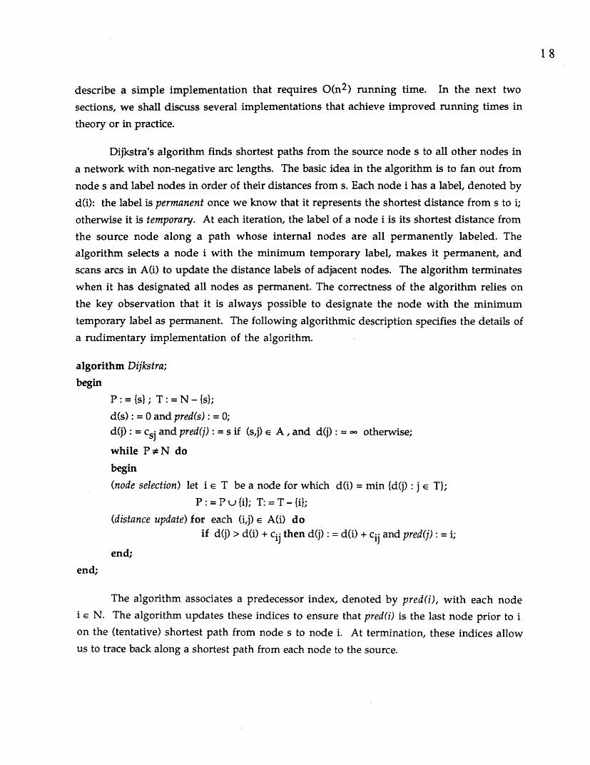
algorithm Dijkstra;

begin

P: = {s}; T:=N-{s};

d(s): = 0 and pred(s) : = 0;

d(j): = Csj and pred(j): = s if (s,j) E A, and d(j): = o otherwise;

while P N do

begin

(node selection) let i E T be a node for which d(i) = min {d(j): j E T};

P: = P u {i}; T: = T- {i};

(distance update) for each (i,j) E A(i) doif d(j) > d(i) + cij then d(j): = d(i) + cij and pred(j): = i;

end;

end;

The algorithm associates a predecessor index, denoted by pred(i), with each node

i e N. The algorithm updates these indices to ensure that pred(i) is the last node prior to i

on the (tentative) shortest path from node s to node i. At termination, these indices allow

us to trace back along a shortest path from each node to the source.

19

The computational time for Dijkstra's algorithm can be split into the time required

by the following two basic steps: (i) node selection; and (ii) distance update. In the most

straightforward implementation, the algorithm performs the node selection step at most n

times and each such step requires examining each temporarily labeled node. Thus the total

time is O(n2 ). The algorithm performs the distance update step I A(i) I times for node i.

Overall, the algorithm performs this step I A(i) I = m times. Each distance updateis N

step takes O(1) time, resulting in O(m) total time for all distance updates. Consequently, this

implementation of Dijkstra's algorithm runs in O(n2 ) time. This time bound is the best

possible for completely dense networks, but can be improved for sparse networks. In thenext two sections we shall discuss several such improvements.

2.2 Heap Implementations

A heap (or priority queue) is a data structure that allows us to perform the following

operations on a collection H of objects, each having an associated real number called its key.

We need to perform the following operations on the heap.

find-min(H): Find and return an object of minimum key.

insert(x, H) : Insert a new object x with predefined key into a collection of objects.

decrease(value, x, H): Reduce the key of an object x from its current value to value, which

must be smaller than the key it is replacing.

delete-min(x, H): Delete an object x of minimum key from the collection H of objects.

If we implement Dijkstra's algorithm using a heap, then H would be the collection

of nodes with finite temporary distance labels and the key of a node would be its distance

label. The algorithm would perform the operation find-min(i, H) to locate a node i with

minimum distance label and perform the operation delete-min(i, H) to delete it from the

heap. Further, while scanning the arc (i, j) in A(i), if the algorithm finds that d(j) = -a, then

it updates d(j) and performs the operation insert(j, H); otherwise, if the distance update step

decreases d(j) to a smaller value, say val, then it performs decrease(val, i, H). Clearly, thealgorithm performs the operations find-min, delete-min and insert at most n times and the

operation decrease at most m times. We now describe the running times of Dijkstra's

algorithm if it is implemented using different data structures.

20

Binary Heap Implementation (Williams [1964]). The binary heap data structure takes O(log

n) time to perform every heap operation. Consequently, a binary heap version of Dijkstra's

algorithm runs in O(m log n) time. Notice that the binary heap implementation is slower

than the original implementation of Dijkstra's algorithm for completely dense networks,

but is faster for sparse networks.

d-Heap Implementation (Johnson [1977a]). For a given parameter d > 2, the d-heap datastructure takes O (logdn) time for every heap operation except delete-min which takes O(dlogdn) time. Consequently, the running time of this version of Dijkstra's algorithm is O(m

logdn + nd logdn). An optimal choice of d occurs when both the terms are equal. Hence, d

= max { 2, rm/nl } and the resulting running time is O(m logdn). Observe that for

completely dense networks (i.e., m = (n 2)) the running time of d-heap implementation isO(n2 ) which is comparable to that of the original implementation, and for very sparsenetworks (i.e., m = O(n)), the running time of d-heap implementation is O(n log n) which is

comparable to that of the binary heap implementation. For networks with intermediate

densities, the d-heap implementation runs faster than both the other implementations.

Fibonacci Heap Implementation (Fredman and Tarjan [1984]). The Fibonacci heap data

structure performs every heap operation in 0(1) amortized (average) time except delete-min

which takes O(log n) time. Hence the running time of this version of Dijkstra's algorithm

is O(m + n log n). This time bound is consistently better that of binary heap and d-heap

implementations for all network densities. This implementation is also currently the best

strongly polynomial algorithm for solving the shortest path problem.

Johnson's Implementation (Johnson [1982]). Johnson's data structure is applicable only

when all arc lengths are integer. This data structure takes O(log log C) time to perform each

heap operation. Consequently, this implementation of Dijkstra's algorithm runs in

O(m log log C). Notice that for problems that satisfy the similarity assumption, Johnson's

implementation is faster than the Fibonacci heap implementation if m < (n log n) /

(log log n) and slower if m > (n log n)/(log log n). Therefore, for Johnson's implementation

to be faster than Fibonacci heap implementation, the network must be very sparse.

Other implementation of Dijkstra's algorithm have been suggested by Johnson

[1977b], van Emde Boas, Kaas and Zijlstra [1977], Denardo and Fox [1979] and Gabow [1985].

21

2.3 Radix Heap Implementation

We now describe a radix heap implementation of Dijkstra's algorithm, whose

running time is comparable to the best algorithm listed previously when applied to

problems satisfying the similarity assumption. The choice of the name radix-heap reflects

the fact that the radix heap implementation exploits properties of the binary representation

of the distance labels. The algorithm we present is a variant of the original radix heap

algorithm presented in Ahuja, Mehlhorn, Orlin, and Tarjan [1988], which in turn extends

an algorithm proposed by Johnson [1977b]. The radix heap algorithm and its analysis

highlight the following key concepts that underlie recent improvements in network flow

algorithms:

(i) How running times might be improved through careful implementation of data

structures.

(ii) How to obtain improved running times by exploiting the integrality of the data and the

fact that the integers encountered are not too large.

(iii) The algorithm and its analysis are relatively simple, especially as compared to other

heap implementations and their analyses.

(iv) The analysis of the radix heap implementation relies on evaluating directly the total

time for two of its operations (find-min and update) rather than the maximum time for a

single iteration. In fact, the maximum time for a given find-min operation is O(n log(nC))

in the implementation we describe, while the sum of the computational times for all find-

mins is also O(n log (nC)); thus, the average time per find-min is O(log (nC)). In order to

establish this time bound, we must adopt a more global perspective in the running time

analysis.

The radix heap implementation relies on the use of buckets for storing nodes. This

idea has also been used in other shortest path algorithms, notably those proposed by Dial

[1969] and by Denardo and Fox [1979]. Before illustrating the radix heap implementation, as

a staring point we first present a very simple bucket scheme algorithm due to Dial [1969].

Suppose that we maintain 1 + nC buckets numbered 0, 1, . . ., nC. Recall that nC is

an upper bound on the length of any path in G, and hence is an upper bound on the

shortest path from node 1 to any other node.

22

Simple Storage Rule. Store a node j with temporary distance label d(j) in bucket numbered

d(j).

This storage rule is particularly easy to enforce. Whenever a temporary label for

node j changes from k to k', we delete node j from bucket k and add it to bucket k'. Each of

these operations takes O(1) steps if we use doubly linked lists to represent nodes in the

buckets. To carry out the find-min operation, we scan the buckets to look for the minimum

non-empty bucket. However, to carry out this operation efficiently, we exploit the

following elementary property of Dijkstra's algorithm.

Observation 2.1. The distance labels that Dijkstra's algorithm designates as permanent are

non-decreasing.

This observation follows from the fact that at every iteration, the algorithm

permanently labels a node i with the smallest temporary distance label d(i), and, since arc

lengths are non-negative, scanning arcs in A(i) during the distance update step does notdecrease the distance label of any node below d(i). Let Pmax denote the maximum distance

label of a permanently labeled node; i.e., it is the distance label d(i) of the node i most

recently designated as permanent. By Observation 2.1, we can search for the minimumnon-empty bucket starting with bucket Pmax. Thus, the total time spent scanning buckets is

O(nC).

The simple storage rule is unattractive from a worst-case perspective since it requires

an exponential number of buckets. (We stress our use of the phrase worst case here.

Although Dial's algorithm has unattractive worst case performance, a minor variant of it is

very effective in practice.) In order to improve the worst case performance, we must

drastically reduce the number of buckets; however, if we are not careful, doing so could lead

us to incur other significant costs. For example, if we could reduce the number of buckets to

one, then in order to find the minimum distance label we would have to scan the contents

of the bucket, and this task would take O(n) per find-min operation. This one bucket

scheme is the same as Dijkstra's original algorithm. Suppose instead that we modified the

simple storage rule so that bucket k stored all nodes whose distance label was in the range

R(k-1) to Rk - 1, for some fixed R > 2. Even if R = 2, it would still take O(n) time to find the

minimum distance labael in a bucket, unless we used more sophisticated data strucutres.

The radix heap algorithm that we discuss next takes an alternate approach: it uses different

sized buckets and stores many, but not all, labels in some buckets.

23

The radix heap algorithm uses only 1 + Flog(nC)l buckets, numbered 0, 1, 2, .. ., K =Flog(nC)l. In order to describe the storage scheme and the algorithm, we first assume thatthe distance labels are stored in binary form. The binary representation is not reallyrequired at an implementation level, but it is helpful for understanding the algorithm.

In order to see how the radix heap storage rule works, let us consider an example.

Suppose at some point in the algorithm, the largest distance label of a permanently labelednode (in binary) is Pmax = 10010 and that nC is 63, or 111111 in binary. We will store

temporary nodes in buckets with the following ranges for their distance labels.

Range(O) = 10010

Range(l) = 10011

Range(2) = 0

Range(3) = 10100,...,10111

Range(4) = 11000,..., 11111

Range(5) = 0

Range(6)= 100000,...,111111.

Thus, if node j has a temporary distance label of d(j) = 10101 (in binary), we store it inbucket number 3. In general, we determine the ranges for the buckets as follows. Bucket 0contains all temporary nodes whose distance label equals Pmax. Any other temporary nodediffers from Pmax in one or more bits. Bucket k for k > 1 contains all of the nodes whoseleftmost difference bit is bit k. The label d(j) we just considered differs from Pmax in both

bits 1 and 3, so we store its node j in bucket number 3.

Radix Heap Storage Rule. For each temporary node j, store node j in bucket k if the node'sdistance label d(j) and Pmax differ in bit k and agree in all bits to the left of bit k.

We can make two immediate observations about this storage scheme.

Observations 2.2.

(a) If Pmax < d(i) < d(j), then node i belongs either to the same bucket as node j or to a lower

numbered bucket.

(b) If the i-th bit of Pmax is 1, then bucket i is empty (for instance, bucket 2 in our example).

24

The first observation follows easily from the radix heap storage rule. The secondobservation follows from the fact the label of every temporarily labeled node is at leastPmax and thus the label of no temporary node can agree with Pmax in every bit to the left ofbit i and have a 0 as its i-th bit.

Now consider the mechanics for performing the find-min step, and for updating thestorage structure as Pmax changes. To carry out the find-min operation, we sequentially

scan buckets to find the lowest indexed non-empty bucket B. (This operation takesO(log(nC)) time per find-min step and O(n log(nC)) time in total.) Having located bucket B,we scan its content in order to select the node i with minimum distance label. We thenreplace Pmax by d(i), and we modify the bucket assignments so that they again satisfy the

radix heap storage rule.

To illustrate the operations needed to carry out the find-min step, suppose that theminimum non-empty bucket from our example is bucket 4. Thus d(i) lies between 11000and 11111. Pmax differs from d(i) in the 4-th bit, and agrees in bit j for j > 4. Thus each nodein a bucket k for k > 5 still satisfies the storage rule when we increase Pmax to value d(i).

The only nodes that shift buckets are those currently in bucket 4, since they agree with d(i)in all bits k for k > 4 and thus differ, if at all, in bit 1,2, or 3. In general, the algorithm

satisfies the following property:

Observation 2.3. Suppose that the node with minimum temporary distance label (asdetermined by the find-min operation) lies in bucket B. Then after the algorithm hasupdated Pmax and enforced the storage rule, each node in bucket B will shift to a smaller

indexed bucket. Every other node stays in the same bucket it was in prior to the find-minstep.

Since we change the label of any node and re-configure the storage of nodes onlyafter the algorithm has updated Pmax, the preceding observation implies the following

result.

Observation 2.4. Whenever a node with a temporary distance label moves to a differentbucket, it always moves to a bucket with a lower index. Consequently, the number of node-shifts is O(n log(nC)) in total.

We have shown that the number of node-shifts is O(n log(nC)). Therefore, toachieve the desired time bound of O(m + n log(nC)) for the algorithm as a whole, we must

25

show that the other operations -- assigning nodes to buckets and finding the node withminimum temporary distance label - do not require any more than this amount of work.First, we show that we need not compute the binary representation of the distance labels.Then we consider the time to find the minimum distance label.

To implement the radix heap implementation, we need not determine the binaryrepresentation of the distance labels. Rather, we can rely solely on the the binaryrepresentation of Pmax. Determining this representation requires O(log(nC)) time, since

the number of bits in any distance label is at most log(nC). Knowing the binaryrepresentation of Pmax, we can then

(i) compute all of the bucket ranges in an additional O(log(nC)) time; and

(ii) determine the bucket for storing node j by sequentially scanning bucket ranges. Forexample, suppose that node j currently lies in bucket B, and that we have just updated itsdistance label d(j). We can determine the new bucket for node j by sequentially scanningthe ranges of buckets B, B-1, B-2, . . . until we locate the bucket whose range contains d(j).For each node j, the number of scanning steps over all iterations is bounded by the numberof buckets plus the number of times that we update d(j). Since the number of updates of d(-)is at most m in total, the running time for re-establishing the radix heap storage rule isO(m + n log(nC)) in total.

Now consider the time spent in the find-min operation. Recall that we first searchfor the minimum indexed non-empty bucket B. This search takes O(log(nC)) time per find-min, or O(n log(nC)) time in total. We must also search B for the minimum distance labeld(i). The time to find the minimum label is proportional to the number of nodes in B,which is bounded by n-1. But this bound is unsatisfactory. However, by Observation 2.3, weknow that each node scanned in bucket B must move after we have replaced Pmax by d(i).

Thus the number of distance labels we scan in the find-min operation is bounded by thenumber of times that nodes change buckets, which is bounded by O(n log(nC)) over alliterations. We have thus proved that the sum of the times to carry out the find-minoperations is O(n log (nC)). Note that establishing this bound requires that we view thealgorithm globally by looking at the relationship among its overall steps; looking at eachcomponent step individually does not provide us with sufficient information to assess thecomputational work this precisely. The analysis of many contemporary network flowalgorithms requires a similar "amortization" approach that bounds the average, rather thanthe maximum amount of work per iteration.

26

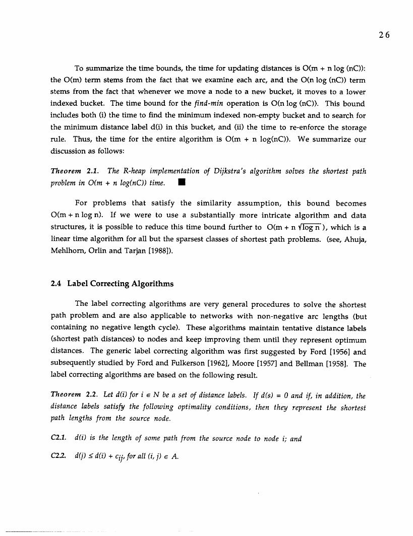
To summarize the time bounds, the time for updating distances is O(m + n log (nC)):the O(m) term stems from the fact that we examine each arc, and the O(n log (nC)) termstems from the fact that whenever we move a node to a new bucket, it moves to a lowerindexed bucket. The time bound for the find-min operation is O(n log (nC)). This boundincludes both (i) the time to find the minimum indexed non-empty bucket and to search forthe minimum distance label d(i) in this bucket, and (ii) the time to re-enforce the storagerule. Thus, the time for the entire algorithm is O(m + n log(nC)). We summarize ourdiscussion as follows:

Theorem 2.1. The R-heap implementation of Dijkstra's algorithm solves the shortest path

problem in O(m + n log(nC)) time. a

For problems that satisfy the similarity assumption, this bound becomes

O(m + n log n). If we were to use a substantially more intricate algorithm and datastructures, it is possible to reduce this time bound further to O(m + n log n ), which is alinear time algorithm for all but the sparsest classes of shortest path problems. (see, Ahuja,

Mehlhorn, Orlin and Tarjan [1988]).

2.4 Label Correcting Algorithms

The label correcting algorithms are very general procedures to solve the shortestpath problem and are also applicable to networks with non-negative arc lengths (butcontaining no negative length cycle). These algorithms maintain tentative distance labels(shortest path distances) to nodes and keep improving them until they represent optimumdistances. The generic label correcting algorithm was first suggested by Ford [1956] andsubsequently studied by Ford and Fulkerson [1962], Moore [1957] and Bellman [1958]. Thelabel correcting algorithms are based on the following result.

Theorem 2.2. Let d(i) for i E N be a set of distance labels. If d(s) = 0 and if, in addition, thedistance labels satisfy the following optimality conditions, then they represent the shortestpath lengths from the source node.

C2.1. d(i) is the length of some path from the source node to node i; and

C2.2. d(j) < d(i) + cij, for all (i, j) E A.

27

Proof. Let P, consisting of the nodes s = i - i2 - ... - ik = j be any directed path from s tosome node j. Condition C2.2 implies that d(i2) < d(i1 ) + cili2 d(i3 ) < d(i2 ) + ci2i3.. .,

n

d(ik) < d(ik-l) + Cik lik. Combining these inequalities yields d(j) = d(ik) < I cij.(i,j)eP

Therefore d(j) is a lower bound on the length of any directed path from s to j including any

shortest path to node j. By condition C2.1, d(j) is an upper bound on the length of the

shortest path. Thus d(j) is the length of a shortest path from node s to node j. ·

The label correcting algorithm is a general procedure for successively updating the

distance labels until they satisfy the condition C2.2. The following algorithmic statement

formally describes a generic version of the label correcting algorithm.

algorithm label correcting;

begin

d(s): = 0 and pred (s): = 0;

d(j): = o for each j E N - (s};while some arc (i, j) satisfies d(j) > d(i) + cij do

begind(j): = d(i) = cij

pred (j): = i;

end;

end;

In general, the label correcting algorithm terminates finitely if there is no negative

cost circuit; however, the proof of finiteness is particularly simple when the data is integral.

Since each d(i) is bounded from above by nC and below by -nC, and each updating of d(i)

decreases it by at least one unit, the algorithm updates d(i) at most 2nC times. Hence the

total number of distance updates is 2n2 C. Since each iteration updates some distance label,

the algorithm performs O(n2 C) iterations. There are a large number of possible

implementations of the label correcting algorithm. Here we present three specific

implementation of the generic label correcting algorithm that exhibit certain nice

properties.

First-In, First-Out (FIFO) Implementation. This implementation maintains a queue, Q, of

all nodes whose shortest path distances are possibly non-optimum. The algorithm removes

__ __1-__··.11 -- _1__1_.-_1.1_1111�------LII�_- .

28

the front node from Q say node i, examines each arc (i, j) in A(i) and checks whether d(j) >d(i) + cij. If so, it changes d(j) to d(i) + cij and adds node j to the rear of Q. The algorithmterminates when Q is empty. It is possible to show (see, e.g., Ahuja, Magnanti and Orlin[1989]) that this algorithm runs in O(nm) time. This is the best strongly polynomial timealgorithm to solve the shortest path problem with arbitrary arc lengths. Bellman [1958]

suggested this FIFO implementation of the label correcting algorithm.

Deque Implementation. A deque is a two sided queue; i.e., it is a data structure that stores aset so that elements can be added or deleted from the front as well as the rear of the set. Thedeque implementation of the label correcting algorithm is the same as the FIFOimplementation with one exception: if the algorithm has examined a node earlier (i.e., thenode is not now in Q but has appeared there before) then it adds the node to the front of Q;otherwise it adds the node to the rear of Q. This implementation does not run inpolynomial time, but has been found in practice to be one of the fastest algorithms forsolving the shortest path problems in sparse networks. D'Esopo and Pape [1974] suggestedthe deque implementation of the label correcting algorithm.

Scaling Label Correcting Algorithm. This recent implementation of the label correctingalgorithm is due to Ahuja and Orlin [1988] and ensures that it alters node labels only ifdoing so decreases them by a sufficiently large amount. The algorithm performs a numberof scaling phases and maintains a parameter A which remains unchanged throughout ascaling phase. Initially A = 2 Flog Ul. In the A-scaling phase, the algorithm updates adistance label d(j) only when d(j) > d(i) + cij + A/2. When no arc satisfies d(j) > d(i) + cij +A/2, then the algorithm replaces A by A/2 and begins a new scaling phase. The algorithm

terminates when A < 1. Ahuja and Orlin show that this version performs O(n2 log C)iterations and can be implemented so that it runs in O(nm log C) time.

3. Maximum Flows

The maximum flow problem is another basic network flow model. Like the shortestpath problem, the maximum flow problem often arises as a subproblem in more complexcombinatorial optimization problems. Moreover, this problem plays an important role insolving the minimum cost flow problem (see Rock [1980], Bland and Jensen [1985], andGoldberg and Tarjan [1987]).

29

The maximum flow problem has an extensive literature. Numerous researchcontributions, many of which often have built upon their precursors, have producedalgorithms with improved worst-case complexity and some of these improvements havealso produced faster algorithms in practice. The first formulation of the maximum flowproblem was given by Ford and Fulkerson [1956], Dantzig and Fulkerson [1956] and Elias,

Feinstein and Shannon [1956], who also suggested algorithms for solving this problem.

Since then researchers have developed many improved algorithms. Figure 3.1 summarizes

the running times of some of these algorithms. In the figure, n is the number of nodes, mis the number of arcs and U is an upper bound on the integral arc capacities. The

algorithms whose time bounds involve U assume integral capacities; the other algorithms

apply to problems with arbitrary rational or real capacities.

In this paper we shall study some of these algorithms, namely,

(i) the basic augmenting path algorithm developed by Ford and Fulkerson [19561;

(ii) the shortest augmenting path algorithm due to Dinic [1970] and Edmonds and

Karp [1972] and as modified by Orlin and Ahuja [1987];

(iii) the capacity scaling algorithm proposed by Gabow [1985] and modified by

Orlin and Ahuja [1987];

(iv) the preflow push algorithms developed by Goldberg and Tarjan [1986]; and

(v) the excess scaling algorithm proposed by Ahuja and Orlin [1987].

# Discoverers

1 Edmonds and Karp [1972]

2 Dinic [1970]

3 Karzanov [1974]

4 Cherkasky [1977]

5 Malhotra, Kumar and Maheshwari [1978]

6 Galil [1980]

7 Galil and Naamad [1980]; Shiloach [1978]

8 Shiloach and Vishkin [1982]

9 Sleator And Tarjan [1983]

10 Tarjan [1984]

11 Gabow [1985]

12 Goldberg [1985]

13 Goldberg and Tarjan [1986]

14 Cheriyan and Maheshwari [1987]

15 Ahuja and Orlin [1987]

Running Time

O(nm2 )

O(n2 m)

O(n3 )

O(n2 {--j)

O(n3 )

O(n5 / 3 m2/3)

O(nm log2 n)

O(n3)

O(nm log n)

O(n3)

O(nm log U)

O(n3)

O(nm log (n 2 /m))

O(n2 -j)

O(nm + n2 log U)

(a) O(nm + n2¥1ogU)

16 Ahuja, Orlin and Tarjan [1988]

17 Cheryian and Hagerup [1989]0(b) nm In log in 2U

O(nm + n 2 log3 n)1

Figure 3.1. Running times of maximum flow algorithms.

We first define some notation. We considerpositive integer capacity uij associated with every arc

two distinguished nodes of the network. A flow x

conditions

a directed network G = (N, A) with a(i, j) E A. The source s and sink t are

is a function x: A -- R satisfying the

1 This is a randomized algorithm. The other algorithms are deterministic.

30

31

Xji - E xij = 0, for all i N -{s, t},{j: (j,i) e A} ) {j: (i,j) A} (3.1a)

C jt V, (3.lb){j: (j, t) Aj (3.1b)

O < xij < uij, for all (i, j)E A, (3.1c)

for some v > 0. We refer to v as the value of flow x. The maximum flow problem is todetermine the maximum possible flow value v and a flow x that achieves this flowvalue.

In considering the maximum flow problem, we impose two assumptions: (i) all arccapacities are finite integers; and (ii) for every arc (i, j) in A, (j, i) is also in A. It is easy toshow that we incur no loss of generality in making these assumptions.

The concept of residual network plays a central role in the discussion of all themaximum flow algorithms we consider. Given a flow x, the residual capacity, rij, of any arc

(i, j) A represents the maximum additional flow that can be sent from node i to node jusing the arcs (i, j) and (j, i). The residual capacity has two components: (i) uij - xij, theunused capacity of arc (i, j), and (ii) the current flow xji on arc (j, i) which can be cancelled toincrease flow from node i to node j. Consequently, rij = uij - xij + xji. We call the network

consisting of only those arcs with positive residual capacities as the residual network (withrespect to the flow x), and represent it as G(x).

Recall from Section 1.3 that a set of arcs Q c A is a cut if the subnetwork G' = (N, A -Q) is disconnected and no subset of Q has this property. A cut partitions the set N into

two subsets. Conversely, any partition of the node set as S and S = N - S defines a cut.

Consequently, we denote an s-t cut as [ S, S ]. A cut [ S, S ] is called an s-t cut if s S and

t S. We define the capacity of an s-t cut as u[S, S] = X _ uij . Each maximum flowieS jS

algorithm that we consider finds both a maximum flow and a cut of minimum capacity.These values are equal, as is well known from the celebrated max-flow min-cut theorem.

Theorem 3.1 (Max-Flow Min-Cut Theorem). The maximum value of flow from s to tequals the minimum capacity of all s-t cuts. U

32

3.1 Generic Augmenting Path Algorithm

A directed path from the source to the sink in the residual network is called an

augmenting path. We define the residual capacity of an augmenting path as the minimumresidual capacity of any arc in the path. Observe that by the definition of an augmenting

path, its capacity is always positive. Hence the presence of an augmenting path implies that

we can send additional flow from source to sink. The generic augmenting path algorithm is

essentially based on this simple idea. The algorithm proceeds by identifying augmenting

paths and augmenting flows on these paths until no such path exists. The following high-level (and flexible) description of the algorithm summarizes the basic iterative steps,without specifying any particular strategy for how to determine augmenting paths.

algorithm augmenting path;

begin

X: = 0;

while G(x) contains a path from s to t do

begin

identify an augmenting P from s to t;8: = min {rij: (i, j) e P;

augment units of flow along P and update G(x);

end;

end;

We now discuss the augmenting path algorithm in more detail. Since an

augmenting path is any directed path from s to t in the residual network, by using any

graph search technique such as the breadth-first search or depth-first search, we can find

one, if the network contains any, in O(m) time. If all capacities are integral, then the

algorithm would increase the value of the flow by at least one unit in each iteration and

hence would terminate in a finite number of iterations. The maximum flow value,

however, might be as large as nU, and the algorithm could perform O(nU) iterations and

take O(nmU) time to terminate. This bound on the number of iterations is not polynomial

for large values of U; e.g., if U = 2 n, the bound is exponential in the number of nodes. We

shall next describe two specific implementations of the generic algorithm that perform a

polynomial number of augmentations.

33

3.2 Capacity Scaling Algorithm

The generic augmenting path algorithm is slow in the worst case because it could

perform a large number of augmentations, each carrying a small flow. Hence, one natural

specialization of the augmenting path algorithm would be to augment flow along a path

with the maximum (or nearly maximum) residual capacity. The capacity scaling algorithm

uses this idea. The capacity scaling algorithm was originally developed by Gabow [19851.

Here, we present a modification of the original algorithm.

The capacity scaling algorithm uses a parameter A. For any given flow x, we define

the A-residual network, G(x, A), as the subnetwork consisting of arcs with residual capacity

of at least A. Initially A = 2rlog U. We refer to a phase of the algorithm during which A

remains constant as a scaling phase, or a A-scaling phase, if we wish to emphasize the

specific value of A. In the A-scaling phase, the algorithm identifies a directed path from s

to t in G(x, A) and augments A units of flow. When G(x, A) contains no augmenting path,

the algorithm replaces A by A/2 and repeats the computations. In the last scaling phase, A

= 1 and hence G(x, A) = G(x). Consequently, at the end of the last scaling phase, the

algorithm terminates with a maximum flow.

The efficiency of the algorithm depends upon the fact that it performs at most 2m

augmentations per scaling phase. To establish this result, consider the flow at the end of the

A-scaling phase. Let x' be this flow and let its flow value be v'. Further, let S be the set of

nodes reachable by a directed path from s in G(x', A). Since G(x', A) contains no

augmenting path from the source to the sink, t o S. Hence (S, S), with S = N - S, is an s-t

cut. The definition of S implies that the residual capacity of every arc in (S, S) is strictly

less than A. Therefore, the residual capacity of the cut (S, S) is at most mA. Consequently,

the maximum flow value v* satisfies the inequality v* - v' < mA. In the next scaling

phase, each augmentation carries at least A/2 units of flow and so this phase can perform at

most 2m augmentations. Since the number of scaling phases is at most Flog Ul, we have

established the following result.

Theorem 3.2. The capacity scaling algorithm solves the maximum flow problem within

O(m log U) augmentations. a

By using a breadth-first-search algorithm, we can identify an augmenting path in

G(x, A) in O(m) time per augmentation for a total running time of O(m2 log U). It is

possible to improve even further on the complexity of the capacity scaling algorithm to

34

O(nm log U) by augmenting flows along shortest paths in G(x, A), as presented by Orlin and

Ahuja [1987].

3.3 Shortest Augmenting Path Algorithm

Another natural specialization of the augmenting path algorithm is to augment flow

along a "shortest path" from the source to the sink, defined as a directed path in the residual

network consisting of the fewest number of arcs. If we always augment flow along a

shortest path, then from one iteration to the next the length of a shortest path either stays

the same or increases. Moreover, as we will see, within m augmentations, the algorithm is

guaranteed to increase the length of a shortest path. Since no path contains more than n-1

arcs, this property guarantees that the number of augmentations are at most (n-l)m. This

algorithm, called the shortest augmenting path algorithm, was independently discovered by

Edmonds and Karp [1972] and Dinic [1970]. Here we shall describe a modified version of the

algorithm developed by Orlin and Ahuja [1987].

It is easy to determine a shortest augmenting path by performing a breadth-first-

search of the residual network. This approach would take O(m) steps per augmentation in

the worst case as well as in the practice. Using the concept of distance labels, described

below, we can reduce the (amortized) average time per augmentation to O(n). Distance

labels were developed for the maximum flow problem by Goldberg [1985] in the context of

preflow push algorithms. They are closely connected to the consept of -complementary

slackness as developed by Bertsekas [1979] and [1986] for the assignment and min cost flow

problems.

Distance Labels

A distance function d: N - Z + with respect to the residual capacities rij is a function

from the set of nodes to the non-negative integers. We say that a distance function is valid

if it satisfies the following two conditions:

C3.1. d(t) = 0;

C3.2. d(i) < d(j) + 1 for every (i, j) E A with rij > 0.

We refer to d(i) as the distance label of node i and condition C3.2 as the validity

condition. The following observations about the distance labels are easy to prove.

35

Observation 3.1. If distance labels are valid then each d(i) is a lower bound on the length of

the shortest (directed) path from node i to node t in the residual network. If for each node

i, the distance label d(i) equals the length of the shortest path from node i to t in the residual

network, then we call the distance labels exact.

Observation 3.2. If d(s) > n, then the residual network contains no path from the source to

the sink.

Admissible Arcs and Admissible Paths

We refer to an arc (i, j) in the residual network as admissible if it satisfies

d(i) = d(j) + 1. Other arcs are inadmissible. We call a path from s to t consisting entirely of

admissible arcs an admissible path. The shortest augmenting path algorithm uses the

following observation.

Observation 3.3. An admissible path is a shortest augmenting path from the source to the

sink.

Every arc (i, j) in an admissible path P satisfies the conditions

(i) rij > 0, and

(ii) d(i)= d(j) + 1.

The first property implies that P is an augmenting path and the second property

implies that if P consists of k arcs then d(s) = k. Since d(s) is a lower bound on the length of

any path from the source to the sink (from Observation 3.1), the path P must be a shortest

path.

The Algorithm

The shortest augmenting path algorithm proceeds by augmenting flows along

admissible paths. It obtains an admissible path by successively building it up from scratch.

The algorithm maintains a partial admissible path, i.e., a path from s to some node i

consisting solely of admissible arcs, and iteratively performs advance or retreat steps from

the last node (i.e., tip) of the partial admissible path, called the current-node. If the current-

node i is incident to an admissible arc (i, j), then we perform an advance step and add arc (i,

j) to the partial admissible path; otherwise, we perform a retreat step and backtrack by one

36

arc. After backtracking one arc, we relabel d(i) = min(l+d(j): rij > 0). There is at least one

admissible arc directed from i after the relabel operation.

We repeat these steps until the partial admissible path reaches the sink node at

which time we perform an augmentation. We repeat this process until the flow ismaximum. We can describe the algorithm formally as follows.

initialize. Perform a (reverse) breadth-first search of the residual network starting with the

sink node to compute distance labels d(i). (If d(s)= oo then quit, since there is no s-t flow.)

Let P = 0 and i = s. Go to advance(i).

advance(i). If the residual network contains no admissible arc (i, j), then go to retreat(i). If

the residual network contains an admissible arc (i, j), then set pred(j): = i and P: = P u {(i, j)}.If j = t then go to augment; otherwise, replace i by j and repeat advance(i).

retreat (i). Update d(i): = min {d(j) + 1: rij > 0 and (i, j) E A(i)). (This operation is called a

relabel step.) If d(s) n, then STOP. Otherwise, if i = s then go to advance(i); otherwise

delete (pred (i), i) from P, replace i by pred(i) and go to advance(i).

augment. Let 6: = min {rij: (i, j) E P). Augment 6 units of flow along P. Set P: = o, i: = s

and go to advance(i).

The shortest augmenting path algorithm uses the following data structure to identify

admissible arcs emanating from a node in the advance steps. Recall that we maintain the

arc list A(i) which contains all arcs emanating from node i. Each node i has a current-arc

which is an arc in A(i) and is the next candidate for testing admissibility. Initially, the

current-arc of node i is the first arc in A(i). Whenever the algorithm has to find an

admissible arc emanating from node i, it tests whether its current-arc is admissible. If not,

then it designates the next arc in the arc list as the current-arc. The algorithm repeats this

process until either it finds an admissible arc or it reaches the end of the arc list. In the latter

case, the algorithm declares that A(i) contains no admissible arc. It then performs a relabel

operation and again designates the first arc in A(i) as the current-arc of node i.

We next give an outline of a proof that the algorithm runs in O(n2 m) time.

37

Lemma 3.1. (a) The algorithm maintains valid distance labels at each step.

(b) Each relabel step increases the distance label of a node by at least one

unit.

Proof Sketch. Perform induction on the number of relabel operations and augmentations. U

Lemma 3.2 Each distance label increases at most n times. Consequently, the total number

of relabel steps is at most n2.

Proof. This lemma follows directly from Lemma 3.1(b) and Observation 3.2. m

Lemma 3.3 . The algorithm performs at most nm/2 augmentations.

Proof. Each augment step saturates at least one arc, i.e., decreases its residual capacity to

zero. Suppose that the arc (i, j) becomes saturated at some iteration, and let d' be the

distance labels at the time of the saturation. Thus d'(i) = d'(j) + 1). Let d" be the distance

labels at the time of the subsquent push in arc (i,j). Prior to the time of this push, we must

have sent flow back from node j to node i, (at which point the distance label of j is d*(j)

d'(i) + 1. For a subsequent push in (i,j), the distance label d"(i) > d*(j) + 1 d'(i) + 2).Hence, between two consecutive saturations of arc (i, j), d(i) increases by at least 2 units.

Consequently, any arc (i, j) can become saturated at most n/2 times and the total number ofarc saturations is no more than nm/2. U

Theorem 3.3. The shortest augmenting path algorithm runs in O(n2 m) time.

Proof. Since each retreat step relabels a node, the total number of retreat steps is O(n2). The

time to perform the retreat/relabel steps is O(n I A(i) I = O(nm). The total augmentationieN

time is O(n2 m) since there are at most nm/2 augmentations and each augmentation

requires O(n) time. The number of advance steps is bounded by the augmentation time

plus the number of retreat steps which is again O(n 2 m). The theorem follows from theseobservations. a

38

3.4 Preflow Push Algorithms

The inherent drawback of augmenting path algorithms is that sending flow along a

path can be computationally expensive, i.e., it takes O(n) time in the worst case. The

preflow push algorithms overcome this drawback and therefore provide dramatic

improvements in worst-case complexity. To understand this point better, consider an

(artificially extreme) example given in Figure 3.2. When we apply any augmenting path

algorithm to this problem, it would discover 10 augmenting paths each of length 10, and

would augment unit flow along each of these paths. But, observe that all of these paths

have the first 8 arcs in common, but still each augmentation traverses this set of arcs. If we

could have pushed 10 units of flow from node 1 to node 9, and then sent a unit flow along

10 different paths of length 2, we would have saved a fair amount of repetitive work in

traversing the common set of arcs. This observation is the essential idea underlying the

preflow push algorithms. Karzanov [1974] suggested the first preflow push algorithm for

the maximum flow problem. The generic distance directed preflow push algorithm we

describe here is due to Goldberg and Tarjan [1986], and this algorithm in turn is based on alayered network preflow push algorithm due to Shiloach and Vishkin [1982].

The preflow push algorithms push flows along individual arcs. These algorithms do

not satisfy the mass balance constraints at intermediate stages. In fact, these algorithms

permit the flow entering a node to exceed the flow leaving the node. In other words, apreflow is a function x: A - R + that satisfies (3.lb), (3.1c), and the following relaxation of

(3.1a).

E Xji E- xij 0, for alli e N- s, t}.{j: (j, i ) (j: (i, j) E A

The preflow push algorithms maintain a preflow at each intermediate stage. For a given

preflow x, we define the excess of each node i E N as

e(i) = I xji - xij.{j: (j, i) E A) {j: (i, j) E A)

We refer to a node with positive excess as an active node. We adopt the convention that

the source and sink nodes are never active. Preflow push algorithms always maintain

optimality of the solution and strive to achieve feasibility. Consequently, the basic step in

this algorithm is to select an active node and try to eliminate its excess by pushing flow to its

neighbors. Since ultimately we want to send flow to the sink, we push flow to the nodes

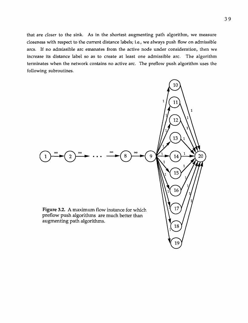
39

that are closer to the sink. As in the shortest augmenting path algorithm, we measure

closeness with respect to the current distance labels; i.e., we always push flow on admissible

arcs. If no admissible arc emanates from the active node under consideration, then we

increase its distance label so as to create at least one admissible arc. The algorithm

terminates when the network contains no active arc. The preflow push algorithm uses the

following subroutines.

Figure 3.2. A maximum flowpreflow push algorithms areaugmenting path algorithms.

40

procedure pre-process;

begin

x: = 0;

compute exact distance labels d(i); (Quit is there is no s-t path with possitive capacity.)Xsj: = Usj for each arc (s, j) E A(s);

d(s): = n;

end;

procedure push/relabel(i);

beginif there is an admissible arc (i, j) then

push 8: = min{e(i), rij} units of flow from node i to node j

else replace d(i) by min {d(j) + 1: (i, j) E A(i) and rij > 01};

end;

A push of units from node i to node j decreases both e(i) and rij by units and

increases both e(j) and rji by units. We say that a push of units of flow on arc (i, j) is

saturating if = rij and non-saturating otherwise. A non-saturating push at node i

reduces e(i) to zero. We refer to the process of increasing the distance label of a node as a

relabel operation. The purpose of the relabel operation is to create at least one admissible

arc on which the algorithm can perform further pushes.

The following generic version of the preflow push algorithm combines the

subroutines just described.

algorithm preflow push;

begin

pre-process;

while the network contains an active node do

begin

select an active node i;

pushlrelabel(i);

end;

end;

It might be instructive to visualize the generic preflow push algorithm in terms of a

physical network whose arcs represent flexible water pipes, nodes represent joints, and the

41

distance function measures how far nodes are above the ground; and in this network, wewish to send water from the source to the sink. In addition, we visualize flow in anadmissible arc as water flowing downhill. Initially, we move the source node upward, andwater flows to its neighbors. In general, water flows downhill toward the sink; however,occasionally flow becomes trapped locally at a node that has no downhill neighbors. At thispoint, we move the node upward, and again water flows downhill toward the sink.Eventually, no flow can reach the sink. As we continue to move nodes upward, theremaining excess flow eventually flows back toward the source. The algorithm terminateswhen all the water flows either into the sink or into the source.

We now indicate how the algorithm keeps track of active nodes for the push/relabelsteps. The algorithm maintains a set S of active nodes. It adds nodes to S that becomeactive following a push and are not already in S, and deletes nodes from S that becomeinactive following a non-saturating push. Several data structures are available for storing Sso that the algorithm can add, delete, or select elements from it in 0(1) time. Further, toidentify admissible arcs emanating from a node, the algorithm uses the current-arc data

structure described earlier for the shortest augmenting path algorithm.

We now analyze the worst case complexity of the generic preflow push algorithm.We first notice that distance labels are always valid and each relabel operation strictly

increases a distance label. The proof of this result is similar to Lemma 3.1 because, as in theshortest augmenting path algorithm, the preflow push algorithm pushes flow only on

admissible arcs and relabels a node only when no admissible arc emanates from it. We alsoneed the following results.

Lemma 3.4. For each i E N, d(i) < 2n.

Proof Sketch. The algorithm relabels only active nodes. The proof amounts to showing

that for each active node i, the residual network contains a path P from node i to node s.The fact that d(s) = n and that d(k ) < d(l) + 1 for every arc (k, 1) in the path implies thatd(i) < d(s)+n-1 < 2n. U

Lemma 3.5. The algorithm performs at most nm saturating pushes.

Proof. Similar to that of Lemma 3.3. a

Lemma 3.6. The algorithm performs O(n2m) non-saturating pushes.

42

Proof. Omitted (See Goldberg and Tarjan [1986]). m

The running time of the generic preflow push algorithm is comparable to the bound

of the shortest augmenting path algorithm. However, the preflow push algorithm has

several nice features, in particular, its flexibility and its potential for further improvements.

By specifying different rules for selecting active nodes for push/relabel steps, we can derive

many different algorithms with different worst-case complexity from the generic version.

The bottleneck operation in the generic preflow push algorithm is the number of non-

saturating pushes; however, many specific rules for examining active nodes substantially

decrease the number of non-saturating pushes. We shall consider the following

implementations: (i) the first-in, first-out (FIFO) preflow push algorithm; (ii) the highest

label preflow push algorithm; and (iii) the excess scaling algorithm.

FIFO Preflow Push Algorithm

Before we describe the FIFO preflow push algorithm, we define the concept of a

node-examination. In an iteration, the generic preflow push algorithm selects a node, say

node i, and performs a saturating push or a non-saturating push or relabels the node. If the

algorithm performs a saturating push, then node i might still be active, but it is not

mandatory for the algorithm to select this node again in the next iteration. The algorithm

may select another node for push/relabel. However, it is easy to incorporate the rule that

whenever the algorithm selects an active node, it keeps pushing flow from that node until

either its excess becomes zero or it is relabeled. Consequently, there might be several

saturating pushes followed either by a non-saturating push or a relabel operation. We refer

to this sequence of operations as a node examination. We shall henceforth assume that the

preflow push algorithms adhere to this rule.

The FIFO preflow push algorithm examines active nodes in the FIFO order. The

algorithm maintains a queue Q of active nodes. It selects a node i from the front of this

queue, performs pushes from this node and adds newly active nodes to the rear of the

queue. The algorithm examines node i until either it becomes inactive or it is relabeled.

In the latter case, we add node i to the rear of the queue. The algorithm terminates when

the queue of active nodes is empty.

For the purpose of analysis, we partition the total number of node examinations into

different phases. The first phase consists of the nodes that become active during the pre-

process step. The second phase consists of all nodes that are in the queue after the

43

algorithm has examined all the nodes in the first phase. Similarly, the third phase consistsof all the nodes that are in the queue after the algorithm has examined all the nodes in thesecond phase, and so on. To bound the number of phases in the algorithm, we consider thetotal change in the potential function F = max d(i): i is active) over an entire phase. If thealgorithm performs no relabel operation in a phase, then the excess of every node that isactive at the beginning of the phase moves to nodes with smaller distance labels, and Fdecreases by at least one unit. However, if the algorithm performs at least one relabeloperation in the phase, then F might increase by as much as the maximum increase in anydistance label. Lemma 3.4 implies that the total increase in F over all the phases is 2n 2.Combining the two cases, we find that the total number of phases is O(n2 ). Each phaseexamines a node at most once. Hence, we have the following result.

Theorem 3.4. The FIFO preflow push algorithm runs in O(n3 ) time. a

Highest Label Preflow Push Algorithm

The highest label preflow push algorithm, also proposed by Goldberg and Tarjan[1986], always pushes flow from an active node with the highest distance label. For thisalgorithm there is a simple proof that the number of non-saturating pushes is O(n3 ).(Cheryian and Maheshwari [1987] improve this elementary bound and show that thenumber of non-saturating pushes is O(n2 Cfl).) Let h* = max {d(i): i is active). We consider asequence of pushes during which no relabel occurs. The algorithm first examines nodeswith distance labels equal to h*. These nodes push flow to nodes with distance label equalto h* - 1, and these nodes, in turn, push flow to nodes with distance label to h* - 2, and soon until either the algorithm has relabeled a node or there are no more active nodes. If anode is relabeled, then the algorithm repeats the same process. But if the algorithm doesnot relabel any node during n consecutive node examinations, then all the excess reachesthe sink (or the source) and the algorithm terminates. Since the algorithm performs atmost 2n2 relabel operations, we immediately obtain a bound of O(n3 ) on the number ofnode examinations. Since each node examination entails at most one non-saturating push,the highest label preflow push algorithm performs O(n3 ) non-saturating pushes and runs inthe same time. As stated, above, Cheriyan and Maheshwari [1987] have improved theanalysis of the algorithm so as to show that the highest label preflow push algorithm has atmost O(n2 i) pushes and runs in the same time.

44

Theorem 3.5. (Cheryian and Maheshwari). The highest label preflow push algorithm

solves the maximum flow problem in O(n 2 fl) time. U

Cheryian and Maheshwari have also shown that this bound is tight in the sense that

for some classes of maximum flow problems, the algorithm actually performs Q (n 2v/- )

computations. In addition, they have shown that for certain suitably chosen networks, the

FIFO preflow push algorithm performs 2(n3) computations and the generic preflow push

algorithm performs Q(n 2m) computations. These interesting results showed that the time

bounds for these three variants of the preflow push algorithm are all tight.

3.5 Excess Scaling Algorithm

The excess scaling algorithm, developed by Ahuja and Orlin [1987], is similar to the

capacity scaling algorithm discussed in Section 3.2. Recall that the generic augmenting path

algorithm performs O(nU) augmentations and the capacity scaling algorithm improves the

number of augmentations to O(m log U) by ensuring that each augmentation carries

"sufficiently large" flow. In the generic preflow push algorithm as well, non-saturating

pushes carrying small amount of flow can in theory be a bottleneck in the algorithm. The

excess scaling algorithm assures that each non-saturating push carries "sufficiently large"

flow so that the number of non-saturating pushes is "sufficiently small."

Let emax = max {e(i): i is active) and let A denote an upper bound on emax. We refer

to A as the excess-dominator. We refer to a node with e(i) > A/2 > emax/ 2 as a node with

large excess, and refer to other nodes as nodes with small excess . The excess scaling

algorithm always pushes flow from a node with large excess. This choice assures that

during non-saturating pushes, the algorithm sends relatively large excess closer to the sink.

The excess scaling algorithm also does not allow the maximum excess to increase

beyond A. This algorithmic strategy might prove to be useful for the following reason.

Suppose several nodes send flow to a single node j, creating a very large excess. It is likely

that node j cannot send the accumulated flow closer to the sink, and thus the algorithm will

need to increase its distance and return much of its excess back to the nodes it came from.

Thus, pushing too much flow to any node is also likely to be wasted effort.

The previous two conditions, namely, that each non-saturating push must carry at

least A/2 units of flow and that no excess should exceed A, imply that we must carefully

45

select the active nodes for push/relabel operations . The following selection rule is one that

ensures the proper behavior:

Node Selection Rule. Among all nodes with large excess, select a node with the smallest

distance label (breaking ties arbitrarily).

We are now in a position to give a formal description of the excess scaling algorithm.

algorithm excess scaling;

begin

pre-process;

A: = 2 Flog U1l

while A > 1 do

begin (A-scaling phase)

while the network contains a node i with large excess do

begin

among all nodes with large excess, select a node i with the

smallest distance label;

perform push/relabel(i) while ensuring that no node excess

exceeds A;

end;

A:=A/2;

end;

end;

The excess scaling algorithm uses the same pushlrelabel(i) step as the genericpreflow push algorithm but with one slight difference. Instead of pushing 6 = min {e(i), rij)

units of flow, it pushes = min {e(i), rij, A - e(j)} units. This change ensures that the

algorithm permits no excess to exceed A.

The excess scaling algorithm performs a number of scaling phases with the value of

the excess-dominator A decreasing from phase to phase. The algorithm performs O(log U)

scaling phases. We now briefly discuss the worst-case complexity of the algorithm.

Lemma 3.7. The algorithm satisfies the following two conditions:

(i) Each non-saturating push sends at least A/2 units of flow.

(ii) No excess ever exceeds A.

_ _____11_1__1__1�^�___�

46

Proof Sketch. The proof uses the facts that for a non-saturating push on arc (i, j), node imust be a node with large excess, node j must be a node with small excess (since node i is anode with large excess with the smallest distance label and d(j) < d(i)), and a push carriesmin {e(i), rij, A - e(j)} flow. U

Lemma 3.8. The excess scaling algorithm performs O(n2 log U) non-saturating pushes.

Proof Sketch. We use the potential function F = I e(i) d(i) / A to prove the lemma.iE N

The potential function increases whenever the scaling phases begins and we replace A byA/2. This increase is O(n2 ) per scaling phase and O(n2 log U) over all scaling phases.

Increasing the distance label of a node i by increases F by at most (because e(i) <A). Thus the total increase in F due to the relabel operations is O(n2 ) over all scaling phases

(by Lemma 3.4). Each non-saturating push carries at least A/2 units of flow to a node with asmaller distance label and hence decreases F by at least A/2 units. These observations give abound of O(n2 log U) on the number of non-saturating pushes. U

Theorem 3.6. The excess scaling algorithm solves the maximum flow problem in O(nm +

n2 log U) time.

Proof. This result follows from Lemma 3.8 and the fact that performing saturating pushes,relabel operations, and finding admissible arcs requires O(nm) time. This accounting

ignores the time needed to identify a large excess node with the smallest distance label.Available simple data structures allow us to perform this computation at an average cost ofO(1) time per push, hence this time is not a bottleneck operation for the algorithm.

3.6 Improved Preflow Push Algorithms

Ahuja, Orlin and Tarjan [1988] have suggested several improved versions of theoriginal excess scaling algorithm. These improvements emerge from the proof of Lemma3.8. This proof bounds the number of non-saturating pushes by estimating the totalincrease in the potential F. Observe that there is an imbalance in this estimate: O(n2 log U)of the increase is due to phase changes, but only O(n2 ) is due to relabelg operations. Ahuja,Orlin and Tarjan improve this estimate by decreasing the contribution of the phasechanges, at the cost of increasing the contribution of the relabel operations. They suggest

47

two algorithms: the stack scaling algorithm and the wave scaling algorithm. The stackscaling algorithm performs O(n2 logU/ log log U) non-saturating pushes and runs in O(nm+ n2 logU/ log log U) time. The wave scaling algorithm performs O(n2 flogU) non-

saturating pushes and runs in O(nm + n2 ¥`logU) time.

Our approach so far has been to reduce the number of non-saturating pushes by

carefully examining the active nodes. An orthogonal approach would be to reduce the total

time of the push operations without necessarily reducing their number. We can achieve

this goal by using the dynamic tree data structure of Sleator and Tarjan [1983]. The

following basic idea underlies the dynamic tree data structure implementation of the

shortest augmenting path algorithm. The shortest augmenting path algorithm repeatedlyidentifies a path consisting solely of admissible arcs and augments flows on these paths.

Each augmentation saturates some arcs on this path. If we delete all the saturated arcs from

this path we obtain a set of path fragments. The dynamic tree data structure stores thesepath fragments (in a very clever way) and uses them later to identify augmenting pathsquickly. Further, this data structure allows the algorithm to augment flow over a pathfragment of length k in O(log k) time.

Ahuja, Orlin and Tarjan [1988] have conjectured that, given a version of the preflow pushalgorithm with a bound of p nm on the total number of non-saturating pushes, therunning time of the algorithm can be reduced from O(p) to O(nm log ((p/nm) +2)) by using

dynamic trees. Although proving such a general theorem is still an open problem,researchers have established this result for each version of the preflow push algorithm

developed so far. For example, Goldberg and Tarjan [1986] improved the running time of

their FIFO preflow push algorithm from O(n3 ) to O(nm log(n2 /m)) and Ahuja, Orlin and

Tarjan [1988] improved the running times of their stack scaling and wave scaling

algorithms to O(nm + log ( n logU ) +2) and O(nm (log (n U) +2)) res-m log logU m

pectively. Recently, Cheryian and Hagerup developed a randomiazed algorithm for solving

the maximum flow problem in O(nm + n2 log3 n) steps. This time bound is the best

strongly polynomial time bound for all networks in which m/n > log 2n.. However, it doesnot dominate the time bound of O(nm + n2 /log U) unless U > nl°g5 n. For example, for n =1000, U must exceed 21,000,000.

48

4. Minimum Cost Flows

The minimum cost flow problem is another core network flow model which is of

considerable theoretical interest and has a great many practical applications. Recent

research contributions, obtained using a number of different algorithmic approaches, have

lead to a series of improvements in the worst-case running times of methods for solving

the minimum cost flow problem. Figure 4.1 reports the running times of some minimum

cost flow algorithms. In the table, n, m, C and U respectively represent the number ofnodes, number of arcs, the largest arc costs and the largest arc capacity in the network. In the

table, S( · ) is the running time of the best shortest path algorithm and M( · ) is the

running time of the best maximum flow algorithm.

Polynomial Time Algorithms

Discoverers Running Time

Edmonds and Karp [1972]

Rock [1980]

Rock [1980]

Bland and Jensen [1985]

Goldberg and Tarjan [1988a]

Goldberg and Tarjan [1988b]

Ahuja, Goldberg, Orlin and Tarjan [1988]

O(m log U S(n, m, C))

O(m log U S(n, m, C))

O(n log C M(n, m, U))

O(n log C M(n, m, C))

O(nm log(n2 /m) log (nC))

O(nm log n log(nC))

O(nm log log U log(nC))

Strongly Polynomial Time Algorithms

Tardos [1985]

Orlin [1984]

Fujishige [1986]

Galil and Tardos [1986]

Goldberg and Tarjan [1988a]

Goldberg and Tarjan [1988b]

Orlin [1988]

O(m4 )

O(m 2 log n S(n, m))

O(m 2 log n S(n, m))

O(n 2 log n S(n, m))

O(nm2 log n log(n2 /m))

O(nm2 log2 n)

O(m log n S(n, m))

Figure 4.1. Polynomial time algorithms for the minimum cost flow problem.

1

2

3

4

5

6

7

1

2

3

4

5

6

7

49

For the sake of comparing the polynomial and strongly polynomial time algorithms

for the shortest path and maximum flow problems, we invoke the similarity assumption.Recall, that the time bounds incorporate the assumption that each arithmetic operationtakes O(1) steps, and this assumption is most appropriate when the numbers satisfy thesimilarity assumption. For problems that satisfy the similarity assumption, the best bounds

for these problems are as follows:

Polynomial Time Bounds

S(n, m, C) = O(min (m log log C, m + n log C))

M(n, m, C) = O(nm log(n o U+ 2))

Strongly Polynomial Time Bounds

S(n, m) = O(m + n log n)

M(n, m) = O(nm log(n2 /m))

or O(nm + n2 log3 n)l

Discoverers

Johnson [1982], and

Ahuja, Mehlhorn, Orlin and

Tarjan [1988]

Ahuja, Orlin and Tarjan [1988]

Discoverers

Fredman and Tarjan [1984]

Goldberg and Tarjan [1986]

Cheryian and Hagerup [1989]

In this paper, we shall discuss some of the algorithms mentioned in the table. Weshall first describe two classical algorithms: the negative cycle algorithm and the successive

shortest path algorithm. We then present two polynomial time algorithms: the RHS-

scaling algorithm based on Edmonds and Karp [1972] scaling technique, and based on thepresentation by Orlin [1988], and the cost scaling algorithm due to Goldberg and Tarjan

[1988a]. We have chosen to discuss these algorithms because they illustrate the ideas of

scaling rather nicely.

1 Recall that this algorithm uses randomization. The other algorithms are deterministic.

50

4.1 Background

We have already given a linear programming formulation (1) of the minimum cost

flow problem. In considering the problem, we make the following assumptions:

(i) all arc costs are non-negative;

(ii) the network connects every pair of nodes by a path of infinite capacity (possibly of

large cost);

(iii) for every pair of nodes i and j, the arc set A does not contain both (i, j) and (j,i).

It is easy to show that the first two assumptions impose no loss of generality. We do

incur some loss of generality by imposing the third assumption of minimum cost flow;

however, we make this assumption solely for notational convenience.

Our algorithms rely on the concept of residual networks. In this section, we define

the residual network G(x) corresponding to a flow x as follows: We replace each arc (i, j) E

A by two arcs (i, j) and (j, i). The arc (i, j) has cost cij and residual capacity rij = uij - xij, and

the arc (j, i) has cost -cij and residual capacity rji = xij. The residual network consists only of

arcs with positive residual capacity.

A dual solution to the minimum cost flow problem is a vector ir of node potentials.

We assume that 7r(1) = 0. The reduced costs c with respect to the node potentials xr aredefined as cij = cij - x(i) + ir(j). A pair x, c of flow and node potentials is optimum if it

satisfies the following linear programming optimality conditions:

C4.1. (Primal Feasibility) x is a feasible flow.

C4.2. (Dual Feasibility) cij > 0 for every arc (i, j) in the residual network G(x).

4.2 Negative Cycle Algorithm

The negative cycle algorithm, attributed to Klein [1967], builds upon the observation

that whenever the residual network contains a negative cycle, we can improve upon the

cost of the current flow by sending additional flow in this cycle. At every iteration, the

algorithm identifies a negative cycle by solving a shortest path problem and augments

maximum possible flow in the cycle. The algorithm terminates when the residual network

contains no negative cycle. This solution is a minimum cost flow.

__ .IIIIIXII·_�._

51

The generic version of the negative cycle algorithm runs in pseudo-polynomial time

since the algorithm improves the objective function value by at least one unit in every

iteration and the maximum possible improvement in the objective function is mCU.

Recently, researchers have suggested the following two polynomial time versions of the

negative cycle algorithm.

(i) Cancelling cycles with maximum improvement. Barahona and Tardos [1987] show that

if the negative cycle algorithm always augments flow along a cycle that gives the maximum

improvement in the objective function, then the algorithm terminates within O(m

log(mCU)) iterations. Since identifying a cycle with maximum improvement is difficult (in

particular, it is NP-hard), they describe a method based upon solving an auxiliary

assignment problem to determine a set of disjoint augmenting cycles with the property thataugmenting flows along these cycles improves the flow cost by at least as much as aug-

menting flow along any single cycle. Their algorithm solves O(m log(mCU)) assignment

problems.

(ii) Cancelling cycles with minimum mean cost. The mean cost of a cycle is its cost divided

by the number of arcs it contains. Goldberg and Tarjan [1988b] showed that if the negativecycle algorithm always augments flow along a cycle whose mean cost is minimum, then the

algorithm performs O(nm min {log(nC), m log n}) iterations. Goldberg and Tarjan also

describe an implementation of a variant of this approach that runs in O(nm log n min{log(nC), m log n}) time.

4.3 Successive Shortest Path Algorithm

The negative cycle algorithm maintains primal feasibility of the solution at every

step and attempts to achieve dual feasibility. In contrast, the successive shortest path

algorithm, as introduced by Busaker and Gowen [1961], maintains dual feasibility of the

solution at every step and strives to attain primal feasibility. This algorithm maintains a

solution that satisfies the non-negativity and capacity constraints, but violates the

supply/demands constraint of the nodes. Such a solution is called a pseudoflow. For anypseudoflow x, we define the imbalance of a node i as

e(i) = b(i) + E xji - Z xij, for all i E N.(j: (j,i) E A) (j: (i, j) E A}

I� �I _ __1_1·ll____lsl^____-----� .�-

52

If e(i) > 0 for some node i, then e(i) is called the excess of node i. If e(i) < 0, then -e(i) is

called its deficit. A node i with e(i) = 0 is called balanced. The residual networkcorresponding to a pseudoflow is defined in the same way that we define the residual

network for a flow. The correctness of the "successive shortest path algorithm" rests on the

following result:

Lemma 4.1. Suppose a pseudoflow x satisfies the dual feasibility condition C4.2 with respect

to the node potentials r. Furthermore, suppose that x' is obtained from x by sending flow

along a shortest path from a node k to a node I in G(x). Let d ( ) denote the shortest path

distances from node k to all other nodes in G(x). Then x' also satisfies the dual feasibilityconditions with respect to the node potentials r - d.

Proof Sketch. Since x satisfies the dual feasibility conditions with respect to the node

potentials r, we have cij > 0 for all (i, j) in G(x). It is possible to show that x also satisfies the

dual feasibility conditions with respect to the node potentials ar' = I - d. Further, the newreduced cost c'ij (defined with respect to the potentials 7') of every arc in the shortest path

from node k to node I is zero. Augmenting flow on any arc (i, j) in this path might add arc(j, i) to the residual network. (The augmentation adds no arcs not on the shortest path.)But since c'ij is zero, c'ji is also zero and so arc (j, i) also satisfies C4.2. U

The successive shortest path algorithm starts with a zero flow and zero node

potentials. At each iteration the algorithm selects a node k with excess and a node I withdeficit, determines shortest path distances d from k to all other nodes, updates node

potentials as 7r = - d, and sends (augments) flow on the shortest path from node k to node

1. The algorithm terminates when the solution satisfies the supply/demand constraint.

The node potentials play a very important role in the successive shortest path

algorithm. Besides using them to prove the correctness of the algorithm, we use them to

ensure that the arc lengths are non-negative, thus enabling us to solve the shortest path

subproblems more efficiently. The successive shortest path algorithm performs O(nU)

iterations since at each iteration it reduces the excess of some node i by at least one unit and

initially e(i) < U. Consequently, we have a pseudo-polynomial bound on the running time

of the algorithm. We next show how to use a scaling technique to make this time bound

polynomial.

53

4.4 Right-Hand-Side (RHS) Scaling Algorithm

The RHS-scaling algorithm is originally due to Edmonds and Karp [1972]. The

version we present here is a modification due to Orlin [1988]. The RHS-scaling algorithm is

a polynomial time version of the successive shortest path algorithm. The inherent

drawback in the successive shortest path algorithm is that augmentations may carry

relatively small amounts of flow, resulting in a fairly large number of augmentations in the

worst case. The RHS-scaling algorithm guarantees that each augmentation carries

sufficiently large flow and thereby reduces the number of augmentations substantially. Weshall illustrate RHS-scaling on the uncapacitated minimum cost flow problem, i.e., aproblem with uij = oo for each (i, j) A. This algorithm can be applied to the capacitated

minimum cost flow problem after it has been converted into an uncapacitated problem

using a standard transformation (see Ahuja, Magnanti and Orlin [1989]). The followingalgorithmic description gives a formal statement of the algorithm.

algorithm RHS-scaling;begin

x: = 0, e: = b;let r be the shortest path distances in G(0);

A = 2log Ul;while the network contains a node with nonzero imbalance dobegin { A-scaling phase}

S(A):= {i E N: e(i) > A};T(A): = {i E N: e(i) < -A);while S(A) • 0 and T(A) * o do

beginselect a node k E S(A) and a node 1 e T(A);determine shortest path distances d() from node k to all other nodes in

the residual network G(x) with respect to the reduced costs cij;

let P denote the shortest path from node k to node 1;update tr: = - d;augment A units of flow along the path P;update x, S(A) and T(A);

end;A: =A/2;

end;end;

The correctness of the RHS-scaling algorithm rests on the following result:

54

Lemma 4.2. The residual capacities of arcs in the residual network are always integer

multiples of A.

Proof. We use induction on the number of augmentations and scaling phases. The initial

residual capacities are a multiple of A because they are either 0 or . Each augmentation

changes the residual capacities by 0 or A units and preserves the inductive hypothesis. A

decrease in the scale factor by a factor of 2 also preserves the inductive hypothesis. m

We next bound the number of augmentations that the algorithm performs. The

algorithm performs a number of scaling phases; we refer to a scaling phase with a specific

value of A as the A-scaling phase. At the beginning of the A-scaling phase, either S(2A) = 0

or T(2A) = o. We consider the case when S(2A) = o. A similar proof applies when T(2A) = 0.

Consequently, at the beginning of the phase, A < e(i) < 2A for each i e S(A). Each

augmentation in the phase starts at a node in S(A), ends at a node with a deficit, and carries

A units of flow (by Lemma 4.2); therefore it decreases I S(A) I by one. Since, initially I S(A) I <

n, the algorithm performs at most n augmentations per phase. Since the algorithm requires

1 + Flog U1 scaling phases, we obtain the following result:

Theorem 4.1. The RHS-scaling algorithm solves the uncapacitated minimum cost flow

problem in O(n log U. S(n, m, C)) time, where S(n, m, C) is the time needed to solve a

shortest path problem with non-negative arc lengths. a

The capacitated problem can be solved in O(m log U S(n, m, C)) time (See Orlin

[1988]). These RHS-scaling algorithms are weakly polynomial since the running times of

algorithms contains a 'log U' term. Orlin, however, has developed a similar strongly

polynomial version of this algorithms that we shall briefly discuss in Section 4.6.

4.5 Cost Scaling Algorithm

We now describe a cost scaling algorithm for the minimum cost flow problem. This

algorithm is due to Goldberg and Tarjan [1988a] and can be viewed as a generalization of the

preflow push algorithm for the maximum flow problem discussed in Section 3.4. The cost

scaling algorithm performs O(log(nC)) scaling phases and within each phase it bears a close

resemblance to the preflow push algorithm for the maximum flow problem. This approach

suggests an important relationship between the maximum flow and minimum cost flow

problem and provides a partial explanation as to why solving the minimum cost flow

55

problem is almost O(log(nC)) times harder than solving the maximum flow problem. We

also note that a non-scaling version of the algorithm is due to Bertsekas [1986].

The cost scaling algorithm relies on the concept of e- optimality. A flow x is said to

be e- optimal for some > 0, if x together with some node potentials r satisfies the following

E- optimality conditions:

C4.3. (Primal Feasibility) x is primal feasible.

C4.4. (Dual Feasibility) cij > - £ for every arc (i, j) in the residual network.

These conditions are a relaxation of the original optimality conditions and reduce toC4.3 and C4.4 when e is zero. The following lemma is useful for analyzing the cost scaling

algorithm.

Lemma 4.3. (Bertsekas [19791. Any feasible flow is &optimal for E2 C. Any e-optimal

feasible flow for e < 1/n is an optimum flow.

Proof. See Bertsekas [1979] (Alternatively, see Ahuja, Orlin, and Magnanti [1988].) U

The cost scaling algorithm treats e as a parameter and iteratively obtains -optimalflows for successively smaller values of E. Initially e = C, and finally e < 1/n. The algorithmperforms cost scaling phases by repeatedly applying an improve-approximation procedurethat transforms an -optimal flow into an e/2-optimal flow. After 1 + log(nC)1 cost scalingphases, < 1/n and the algorithm terminates with an optimum flow. In the improve-

approximation procedure we say that an arc (i, j) is admissible if - < cij < 0 and inadmissible

otherwise. More formally, we can state the algorithm as follows.algorithm cost-scaling;

begin

ic: = 0 and e: = C;

let x be any feasible flow;

while e > 1 /n do

begin

improve-approximation (, x, it);

: = E/2;

end;

x is an optimum flow for the minimum cost flow problem;

end;

56

procedure improve-approximation(, x, 7i);

beginif ij > O then xij:= 0

else if cij < 0 then xij := uij;

compute node imbalances;

while the network contains an active node (i.e., node with positive excess) do

begin

select an active node i;

pushlrelabel(i);

end;

end;

procedure push/relabel(i);

begin

if the network contains an admissible arc (i, j) thenpush 6 = min (e(i), rij} units of flow from node i to node j

else replace nr(i) by r(i) + e/2;

end;

As in our earlier discussion of preflow push algorithms for the maximum flowproblem, if 6 = rij then we refer to the push as saturating; otherwise it is non-saturating.

We also refer to the updating of the potential of a node as a relabel operation. The purpose

of a relabel operation is to create new admissible arcs. Moreover, we use the same data

structure used in the maximum flow algorithms to identify admissible arcs. For each node

i, we maintain a current arc (i, j) which is the current candidate for pushing flow out of the

node i. The current arc is found by sequentially scanning the arc list A(i).

The correctness of the cost scaling algorithm rests on the following results:

Lemma 4.4. The improve-approximation procedure always maintains 4e2-optimality of the

pseudoflow, and at termination yields an E12-optimal flow.

Proof Sketch. First show that the adjustment of arc flows at the beginning of the procedure

yields an E/2-optimal pseudoflow (in fact, it is a O-optimal pseudoflow). Then perform

induction on the number of pushes and relabel steps. U

57

In the last scaling phase, < 1/n and by Lemma 4.3, we obtain an optimum flow ofthe minimum cost flow problem. We now analyze the worst-case complexity of the costscaling algorithm. The complexity analysis uses the following lemma which is ageneralization of Lemma 3.2 and Lemma 3.3 in the context of the maximum flow problem.Lemma 4.5. (Goldberg and Tarjan [1987].) (a) The improve-approximation procedurerelabels a node O(n) times and hence performs O(n2 ) relabel operations in total.

(b) The improve-approximation procedure performs O(nm) saturating pushes.

Proof. Omitted. a

As in the generic preflow push algorithm for the maximum flow problem, thebottleneck operation in the improve-approximation procedure is the number of non-saturating pushes. It is possible to show that the generic version of the improve-approximation procedure, i.e., a version that permits us to select active nodes in anyarbitrary order for the push/relabel operations, performs O(n2 m) non-saturating pushes.Here we shall describe a specific implementation of the generic version, called the waveimplementation that performs O(n3 ) non-saturating pushes per execution of the procedure.Goldberg [1987] and Bertsekas and Eckstein [1988] independently developed thisimplementation of the cost-scaling preflow-push algorithm. The following result is crucialto the analysis of the wave implementations.

Lemma 4.6. The admissible network, i.e., the subnetwork consisting of all admissible arcs inthe network, is acyclic throughout the improve-approximation procedure.

Proof Sketch. One can show that the admissible network at the beginning of the procedure(after adjustments of arc flows) contains no arc and, hence, is acyclic. One then performinduction of the number of relabels and pushes. a

The wave implementation uses the fact that the admissible network is acyclic. As iswell known, nodes of an acyclic network can be numbered in a so called topological order,that is, so that v < w for each arc (v, w) in the network. Determining a topological order isrelatively easy and requires O(m) time. The wave implementation maintains a list of allnodes, LIST, in the topological order irrespective of whether nodes are active or not. Itexamines each node in LIST in the topological order. If the currently chosen node is active,the algorithm performs a push/relabel step on this node until the node either (i) gets rid ofits excess, or (ii) is relabeled. In the former case, the algorithm examines the next node inthe topological order. In the latter case, the relabel of node v changes the admissible

58

network as well as the topological ordering. However, it is possible to show that if we move

node v from its current position in LIST to the first position, then nodes are again

topologically ordered with respect to the new admissible network. The algorithm again

starts examining nodes in LIST in order, starting at the first position.

Observe that if the algorithm has performed no relabel operations as it examined

nodes in LIST, then all active nodes have discharged their excesses and the pseudoflow has

become a flow. This result follows from the fact that when the algorithm examines nodes

in the topological order, active nodes always push flow to higher numbered nodes, which

in turn push flow to higher numbered nodes, and so on. Since the algorithm relabels nodes

O(n2 ) times, we immediately obtain an O(n3 ) bound on the number of node examinations.

Each node examination generates at most one non-saturating push. Consequently, the

wave implementation of the improve-approximation procedure performs O(n3 ) non-

saturating pushes. Since all other steps take O(nm) time per execution of the improve-

approximation procedure and the algorithm calls this procedure O(log(nC)) times, we

obtain the following result.

Theorem 4.2. The wave variant of the cost scaling algorithm solves the minimum cost

flow problem in O(n3 log(nC)) time. U

Researchers have developed several improvements of the cost scaling algorithm.

Using both finger tree (see, e.g., Mehlhorn [1984]) and dynamic tree data structures, Goldberg

and Tarjan [1988a] obtain an O(nm log(n2 /m) log(nC)) bound for the cost scaling algorithm.

For completely dense networks, the wave algorithm has the advantage of

simultaneously being simple and very efficient. Unfortunately, the algorithm is

increasingly less efficient as the network gets sparser and sparser. Fortunately, if the

network is sparse, there is another simple algorithm that achieves a running time that is

nearly O(log nC) times the running time for a maximum flow algorithm. This variant of

the cost-scaling algorithm is due to Ahuja, Goldberg, Orlin and Tarjan [1988] and is called

the double scaling algorithm.

The double scaling algorithm combines ideas from both the RHS-scaling and cost

scaling algorithms and obtains an improvement not obtained by either algorithm alone.

The double scaling algorithm is the same as the cost scaling algorithm discussed in the

previous section except that it uses a more efficient version of the improve-approximation

procedure. The improve-approximation procedure in the previous section relied on a

60

arc whose flow exceeds 2nA at any point during the A-scaling phase will have positive flow

at each subsequent iteration. A natural operation would then be to contract (or shrink) anysuch arc and continue the scaling procedure on a problem involving fewer nodes. (Tardos[1985] developed a dual approach to the one presented here. Fujishige [1986] and Orlin [1984]used a similar approaches for their algorithms.) The strongly polynomial algorithm uses

the fact that within O( log n) scaling phases, we can always contract a new arc. Since we canperform the contraction at most n times, the algorithm performs O( n log n) scaling phases.However, the significant reduction in the running time is to reduce the number of shortest

path computations performed by the algorithm in these phases to O(n log n). Toaccomplish the reduction in the number of shortest path computations, we can modify the

RHS-scaling algorithm as follows:

1. If all of the flows in the (contracted) network are 0, then set A = max (e(i): i E N).

2. The algorithm finds a shortest path from a node i with e(i) > 2A/3 to a node j

with e(j) < -2A/3. (In the RHS scaling algorithm, the path would have been

from a node with excess > A to a node with "excess" < -A.)

3. The algorithm contracts any arc (i,j) for which the flow exceeds 3nA.

The modifications of the RHS-scaling algorithm are quite modest; nevertheless, theproof of the O(n log n) bound on the number of shortest path computations is relativelycomplex. However, the essence of the proof is as follows. We refer to a node i as "active"during the A-scaling phase if it is involved in an augmentation, i.e., A units of flow are sent

on a shortest path starting or ending at node i during the phase. It is possible to show that

the number of augmentations is at most the sum of the number of active nodes taken overall phases. Moreover, it is possible to show show that any active node is contracted (i.e.,incident to a contracted arc) within 3 log n scaling phases. Since there are at most ncontractions throughout the algorithm, this bounds the sum of the number of active nodesat O(n log n) and thus implies a bound of O(n log n) on the number of shortest pathcomputations.

The capacitated problem with n nodes and m arcs may be transformed into anuncapacitated problem with (m + n) nodes and 2m arcs through a standard technique ofinserting a node into the "middle" of each arc. Thus the strongly polynomial algorithm forthe uncapacitated problem yields a strongly polynomial algorithm for the capacitatedproblem, whose running time is O(m log n (m + n log n)). Orlin [1988] provides the detailsof this algorithm and the proof of its complexity.

59

pseudoflow push method. The double scaling algorithm relies on an augmenting path

based method instead. This approach sends flow from a node with excess to a node with

deficit over an admissible path, i.e., a path in which each arc is admissible.

The double scaling algorithm also incorporates ideas from the RHS-scaling

algorithm so as to reduce the number of augmentations to O(n log U) for an uncapacitated

problem by ensuring that each augmentation carries sufficiently large flow. This approach

gives us an algorithm that does cost scaling in the outer loop and within each cost scaling

phase performs a number of RHS-scaling phases; hence, this algorithm is called the double

scaling algorithm. A simple version of the double scaling algorithm runs in

O((nm log U/loglog U) log(nC)) time, which would be the best polynomial bound to solve

the (capacitated) cost flow problem for non-dense problem classes satisfying the similarity

assumption. However, Ahuja, Goldberg, Orlin and Tarjan showed how to improve the

running time by a further factor of O(logU/(loglogU) 2) by incorporating the dynamic tree

data structure.

4.6 A Strongly Polynomial Algorithm

We shall now briefly discuss the strongly polynomial algorithm due to Orlin [1988]

which is currently the best strongly polynomial algorithm for solving the minimum cost

flow problem. This algorithm is an improvement of the RHS-scaling algorithm described

in Section 4.4. This algorithm improves on the other strongly polynomial algorithms

given in Figure 4.1.

The RHS-scaling algorithm is weakly polynomial because its worst case bound

contains the term 'log U' which is the number of scaling phases it performs. For

exponentially large values of U, the number of scaling phases might not be bounded by any

polynomial function of n and m. For example, if U = 2 n, then the algorithm performs n

scaling phases. Orlin [1988] uses several ideas found in the RHS-scaling algorithm to

convert the 'log U' term to 'log n' so that the algorithm becomes strongly polynomial. The

key idea is in identifying arcs whose flow is so large in the A-scaling phase, that they are

guaranteed to have positive flow in all subsequent phases. In the A-scaling phase, the flow

in any arc can change by at most nA units, since there are at most n augmentations and each

augmentation carries A units of flow. If we sum the changes in flow in any arc over all

scaling phases, the total change is at most n(A + A/2 + A/4 + ... 1) = 2nA. Consequently, any

61

Acknowldgement

The research of the first and third authors was supported in part by the Presidential

Young Investigator Grant 8451517-ECS of the National Science Foundation, by Grant

AFORS-88-0088 from the Air Force Office of Scientific Research, and by Grants from Analog

Devices, Apple Computer, Inc., and Prime Computer.

References

Ahuja, R.K., A.V. Goldberg, J.B. Orlin, and R.E. Tarjan. 1988. Finding Minimum-Cost Flows

by Double Scaling. Working Paper No. 2047-88, Sloan School of Management, M.I.T.,

Cambridge, MA.

Ahuja, R.K., T.L. Magnanti and J.B. Orlin. 1989. Network Flows, in Handbooks in

Operations Research and Management Science, Vol. I: Optimization.

Ahuja, R. K., T. L. Magnanti and J. B. Orlin. Network Flows: Theory and Algorithms. To

appear.

Ahuja, R.K., K. Mehlhorn, J.B. Orlin, and R.E. Tarjan. 1988. Faster Algorithms for the

Shortest Path Problem. Technical Report No. 193, Operations Research Center, M.I.T.,

Cambridge, MA. To appear in J. of ACM.

Ahuja, R.K., and J.B. Orlin. 1987. A Fast and Simple Algorithm for the Maximum Flow

Problem. Working Paper 1905-87, Sloan School of Management, M.I.T., Cambridge, MA.

1987. To appear in Oper. Res.

Ahuja, R.K., and J.B. Orlin. 1988. Improved Primal Simplex Algorithms for the Shortest

Path, Assignment and Minimum Cost Flow Problems. Working Paper 2090-88, Sloan

School of Management, M.I.T., Cambridge, MA.

Ahuja, R.K., J.B. Orlin, and R.E. Tarjan. 1988. Improved Time Bounds for the Maximum

Flow Problem. Working Paper 1966-87, Sloan School of Management, M.I.T., Cambridge,

MA. To appear in SIAM J. of Comput.

Barahona, F., and E. Tardos. 1987. Note on Weintraub's Minimum Cost Flow Algorithm.

Research Report, Dept. of Mathematics, M.I.T., Cambridge, MA.

62

Bellman, R. 1958. On a Routing Problem. Quart. Appl. Math. 16, 87-90.

Bertsekas, D.P. 1979. A Distributed Algorithm for the Assignment Problem. Working

Paper, Laboratory for Information Decision Systems, M.I.T., Cambridge, MA.

Bertsekas, D.P. 1986. Distributed Relaxation Methods for Linear Network Flow Problems.

Proc. of 25th IEEE Conference on Decision and Control, Athens, Greece.

Bertsekas, D.P., and J. Eckstein. 1988. Dual Coordinate Step Methods for Linear Network

Flow Problems. To appear in Math. Prog., Series B.

Bland, R.G., and D.L. Jensen. 1985. On the Computational Behavior of a Polynomial-Time

Network Flow Algorithm. Technical Report 661, School of Operations Research and

Industrial Engineering, Cornell University, Ithaca, N.Y.

Busaker, R.G., and P.J. Gowen. 1961. A Procedure for Determining a Family of

Minimal-Cost Network Flow Patterns. O.R.O. Technical Report No. 15, Operational

Research Office, John Hopkins University, Baltimore, MD.

Cheriyan, J., and S.N. Maheshwari. 1987. Analysis of Preflow Push Algorithms for

Maximum Network Flow. Technical Report, Dept. of Computer Science and Engineering,

Indian Institute of Technology, New Delhi, India.

Cherkasky, R.V. 1977. Algorithm for Construction of Maximum Flow in Networks with

Complexity of O(V2 ~4 ) Operation, Mathematical Methods of Solution of Economical

Problems 7, 112-125 (in Russian).

Dantzig, G.B. 1960. On the Shortest Route through a Network. Man. Sci. 6, 187-190.

Dantzig, G.B., and D.R. Fulkerson. 1956. On the Max-Flow Min-Cut Theorem of Networks.

In H.W. Kuhn and A.W. Tucker (ed.), Linear Inequalities and Related Systems, Annals of

Mathematics Study 38, Princeton University Press, 215-221.

Denardo, E.V., and B.L. Fox. 1979. Shortest-Route Methods: 1. Reaching, Pruning and

Buckets. Oper. Res. 27, 161-186.

Dial, R. 1969. Algorithm 360: Shortest Path Forest with Topological Ordering. Comm.

ACM 12, 632-633.

63

Dijkstra, E. 1959. A Note on Two Problems in Connexion with Graphs. Numeriche

Mathematics 1, 269-271.

Dinic, E.A. 1970. Algorithm for Solution of a Problem of Maximum Flow in Networks with

Power Estimation, Soviet Math. Dokl. 11, 1277-1280.

Edmonds, J., and R.M. Karp. 1972. Theoretical Improvements in Algorithmic Efficiency for

Network Flow Problems. J. ACM 19, 248-264.

Elias, P., A. Feinstein, and C.E. Shannon. 1956. Note on Maximum Flow Through a

Network. IRE Trans. on Infor. Theory IT-2, 117-119.

Ford, L.R., Jr. 1956. Network Flow Theory. Report P-923, Rand Corp., Santa Monica, CA.

Ford, L.R., Jr., and D.R. Fulkerson. 1956. Maximal Flow through a Network. Canad. J.

Math. 8, 399-404.

Ford, L.R., Jr., and D.R. Fulkerson. 1962. Flows in Networks.. Princeton University Press,

Princeton, NJ.

Fredman, M.L., and R.E. Tarjan. 1984. Fibonacci Heaps and Their Uses in Improved

Network Optimization Algorithms. 25th Annual IEEE Symp. on Found. of Comp. Sci,

338-346, also in J. of ACM 34(1987), 596-615.

Fujishige, S. 1986. An O(m3 log n) Capacity-Rounding Algorithm for the Minimum Cost

Circulation Problem: A Dual Framework of Tardos' Algorithm. Math. Prog. 35, 298-309.

Gabow, H.N. 1985. Scaling Algorithms for Network Problems. J. of Comput. Sys. Sci. 31,

148-168.

Galil, Z. 1980. O(V5 / 3 E2 / 3 ) Algorithm for the Maximum Flow Problem, Acta Informatica

14, 221-242.

Galil, Z., and A. Naamad. 1980. An O(VE log2 V) Algorithm for the Maximum Flow

Problem. J. of Comput. Sys. Sci. 21, 203-217.

Galil, Z., and E. Tardos. 1986. An O(n2 (m + n log n) log n) Min-Cost Flow Algorithm.

Proc. 27th Annual Symp. on the Found. of Comp. Sci. , 136-146.

___�__��

64

Goldberg, A.V. 1985. A New Max-Flow Algorithm. Technical Report MIT/LCS/TM-291,

Laboratory for Computer Science, M.I.T., Cambridge, MA.

Goldberg, A.V. 1987. Efficient Graph Algorithms for Sequential and Parallel Computers.

Ph.D. Thesis. Department of Electrical Engineering and Computer Science. MIT

Goldberg, A.V., S.A. Plotkin, and E. Tardos. 1988. Combinatorial Algorithms for the

Generalized Circulation Problem. Research Report, Laboratory for Computer Science,

M.I.T., Cambridge, MA.

Goldberg, A.V., E. Tardos, and R.E. Tarjan. 1989. Network Flow Algorithms. Manuscript.

Goldberg, A.V., and R.E. Tarjan. 1986. A New Approach to the Maximum Flow Problem.

Proc. 18th ACM Symp. on the Theory of Comput., 136-146.

Goldberg, A.V., and R.E. Tarjan. 1987. Solving Minimum Cost Flow Problem by Successive

Approximation. Proc. 19th ACM Symp. on the Theory of Comp..

Goldberg, A.V., and R.E. Tarjan. 1988a. Solving Minimum Cost Flow Problem by

Successive Approximation. (A revision of Goldberg and Tarjan [1987].) To appear in Math.

of Oper. Res.

Goldberg, A.V., and R.E. Tarjan. 1988b. Finding Minimum-Cost Circulations by Canceling

Negative Cycles. Proc. 20th ACM Symp. on the Theory of Comp., 388-397.

Johnson, D. B. 1977a. Efficient Algorithms for Shortest Paths in Sparse Networks. J. ACM

24, 1-13.

Johnson, D. B. 1977b. Efficient Special Purpose Priority Queues. Proc. 15th Annual

Allerton Conference on Comm., Control and Computing, 1-7.

Johnson, D. B. 1982. A Priority Queue in Which Initialization and Queue Operations Take

O(log log D) Time. Math. Sys. Theory 15, 295-309.

Karzanov, A.V. 1974. Determining the Maximal Flow in a Network by the Method of

Preflows. Soviet Math. Doklady 15, 434-437.

Klein, M. 1967. A Primal Method for Minimal Cost Flows. Man. Sci. 14, 205-220.

�1_1·1_ ^_ _I II� _I __ ���I�

65

Malhotra, V. M., M. P. Kumar, and S. N. Maheshwari. 1978. An O(I V I 3 ) Algorithm for

Finding Maximum Flows in Networks. Inform. Process. Lett. 7, 277-278.

Mehlhorn, K. 1984. Data Structures and Algorithms. Springer-Verlag.

Moore, E. F. 1957. The Shortest Path through a Maze. In Proceedings of the International

Symposium on the Theory of Switching Part II; The Annals of the Computation Laboratory

of Harvard University 30, Harvard University Press, 285-292.

Orlin, J. B. 1984. Genuinely Polynomial Simplex and Non-Simplex Algorithms for the

Minimum Cost Flow Problem. Technical Report No. 1615-84, Sloan School of

Management, M.I.T., Cambridge, MA.

Orlin, J. B. 1988. A Faster Strongly Polynomial Minimum Cost Flow Algorithm. Proc. 20th

ACM Symp. on the Theory of Comp., 377-387.

Orlin, J. B., and R. K. Ahuja. 1987. New Distance-Directed Algorithms for Maximum Flow

and Parametric Maximum Flow Problems. Working Paper 1908-87, Sloan School of

Management, Massachusetts Institute of Technology, Cambridge, MA.

Pape, U. 1974. Implementation and Efficiency of Moore-Algorithms for the Shortest Route

Problem. Math. Prog. 7, 212-222.

Rock, H. 1980. Scaling Techniques for Minimal Cost Network Flows. In V. Page (ed.),

Discrete Structures and Algorithms . Carl Hansen, Munich, 101-191.

Shiloach, Y., 1978. An O(nI log 2(I)) Maximum Flow Algorithm. Technical Report STAN-

CS-78-702, Computer Science Dept., Stanford University, CA.

Shiloach, Y., and U. Vishkin. 1982. An O(n2 log n) Parallel Max-Flow Algorithm. J.

Algorithms 3 , 128-146.

Sleator, D. D., and R. E. Tarjan. 1983. A Data Structure for Dynamic Trees, J. Comput. Sys.

Sci. 24, 362-391.

Tardos, E. 1985. A Strongly Polynomial Minimum Cost Circulation Algorithm.

Combinatorica 5, 247-255,

___ __ I

66

Tarjan, R. E. 1984. A Simple Version of Karzanov's Blocking Flow Algorithm, Oper. Res.

Letters 2, 265-268.

Van Emde Boas, E. P., R. Kaas, and E. Zijlstra. 1977. Design and Implementation of an

Efficient Priority Queue. Math. Sys. Theory 10, 99-127.

Whiting, P. D., and J. A. Hillier. 1960. A Method for Finding the Shortest Route Through a

Road Network. Oper. Res. Quart. 11, 37-40.

Williams, J. W. J. 1964. Algorithm 232: Heapsort. Comm. ACM 7, 347-348.

I __ _ __ 1 (·11^ .- · --