AFRL-SR-AR-TR-05-

O2S&

REPORT DOCUMENTATION PAGE OMB Noo074-0188Public reporting burden for this collection of information is estimated to average 1 hour per response, including the time for reviewing instructions, searching existing data sources, gathenng and maintainingthe data needed, and completing and reviewing this collection of information. Send comments regarding this burden estimate or any other aspect of this collection of information, including suggestions forreducing this burden to Washington Headquarters Services, Directorate for Information Operations and Reports, 1215 Jefferson Davis Highway, Suite 1204, Arlington, VA 22202-4302, and to the Office ofManagement and Budget, Paperwork Reduction Project (0704-0188), Washington, DC 20503

1. AGENCY USE ONLY (Leave 2. REPORT DATE 3. REPORT TYPE AND DATES COVEREDblank) 0510612005 Final Performance Report, 02/01/03-12/31/044. TITLE AND SUBTITLE 5. FUNDING NUMBERSDesign Tools for Zero Net Mass Flux Devices: CFD Effort F49620-03-1-0146

6. AUTHOR(S)Rajat Mittal, PhD

7. PERFORMING ORGANIZATION NAME(S) AND ADDRESS(ES) 8. PERFORMING ORGANIZATIONREPORT NUMBER

The George WashingtonUniversity801 2 2 nd St. NWWashington DC 20052

9. SPONSORING / MONITORING AGENCY NAME(S) AND ADDRESS(ES) 10. SPONSORING / MONITORINGAGENCY REPORT NUMBER

AFOSR4015 Wilson BoulevardRoom 713 NA -Arlington VA 22203-1954

11. SUPPLEMENTARY NOTES

12a. DISTRIBUTION I/AVAILABILITY STATEMENT 12b. DISTRIBUTION CODEApproved for public release; distribution unlimited.

13. ABSTRACT (Maximum 200 Words)

Numerical simulations have been used to examine the fluid dynamics of zero-net mass flux devices. The emphasis is onextracting insights that can be used in developing simple models of these actuators for use in separation control. Theunsteady evolution of a transitional synthetic jet in the absence of cross-flow is investigated by time-accurate three-dimensional direct numerical simulations of incompressible Navier-Stokes equations and the results compared with one ofthe test cases designated for the NASA CFD Validation of Synthetic Jets and Turbulent Separation Control. The validatedresults are then used for a comprehensive analysis of the flow inside the cavity and the jet slot. The flux of vorticity fromthese devices is considered to be an important factor in the control of separated flow and in the current study, we have usednumerical simulations to extract scaling laws for this quantity. A theoretical model is also proposed for determining thepressure losses in ZNMF slots and orifices and numerical simulations used to determine the scaling of some of the keyparameters in this theoretical model.

14. SUBJECT TERMS 15. NUMBER OF PAGES32

Flow Control, Synthetic jets, Computational Fluid Dynamics 16. PRICECODE

17. SECURITY CLASSIFICATION 18. SECURITY CLASSIFICATION 19. SECURITY CLASSIFICATION 20. LIMITATION OF ABSTRACTOF REPORT OF THIS PAGE OF ABSTRACT UU

Unclassified Unclassified UnclassifiedNSN 7540-01-280-5500 Standard Form 298 (Rev. 2-89)

Prescribed by ANSI Std. Z39-18298-102

20050715 006 1

• p

I. Objectives

1. Simulate 3-D, incompressible, local interaction of a synthetic jet with a boundary layer.Guidance for test cases will be taken from test cases designated for LaRC workshop on"CFD Validation of Synthetic Jets and Turbulent Separation Control."

2. Develop in coordination with experimental team at University of Florida, reduced ordermodels and scaling laws for Zero Net Mass Flux Devices.

II. Introduction

With the onset of MEMS (Micro-Electromechanical Systems) technology the field of active flowcontrol was presented with a promising opportunity of application of the micro/meso devices.Over the past decade ZNMF (Zero-net mass flux) actuators or synthetic jets, as they arepopularly known, have emerged as versatile actuators with potential applications ranging fromthrust vectoring ofjets (Smith & Glezer, 1997), mixing enhancement (Chen et al., 1999; Davis &Glezer, 1999), heat transfer enhancement (Smith et al., 1998; Crook et al., 1999) to triggeringturbulence in boundary layers (Rathnasingham & Breuer, 1997, 2003; Lee & Goldstein, 2001)and active flow control (Wygnanski, 1997; Smith et al, 1998b; Amitay et al, 1999; Crook et al.,1999). The versatility of these actuators is primarily attributed to the following reasons: (a) theyprovide unsteady forcing that is more effective than steady or pulsed forcing, (b) since the jetsare synthesized from the working fluid, complex fluid circuits are not required, and (c) actuationfrequency can usually be tuned to a particular flow configuration.

A typical synthetic jet actuator consists of a jet orifice opposed on one side by an enclosed cavityconsisting of three components: an oscillatory driver, a cavity and an orifice or slot. Theoscillating driver compresses and expands the fluid in the cavity by alternating the cavity volumeat an exciting frequency to create oscillations. These time-periodic changes in volume of thecavity cause a stream of vortices to be generated at the edges of the orifice, imparting finitemomentum into the surrounding fluid, although the net mass-flux through the orifice is zero.Interaction of these vortical structures with the external flow field has been found to causeformation of closed recirculation regions with the modification of the flow boundary, therebycausing global modifications to the base flow on scales larger than the characteristic lengthscales of the synthetic jets themselves (Smith & Glezer, 1997; Amitay et al, 1997). Bothexperimental and numerical investigations have been carried out for synthetic jets operating in aquiescent medium and one interacting with an external boundary for afore mentionedapplications. However, several questions remained unanswered in terms of the fundamental flowphysics governing these flows.

In Section 11(a), the unsteady evolution of a transitional synthetic jet in the absence of cross-flowis investigated by time-accurate three-dimensional direct numerical simulations ofincompressible Navier-Stokes equations. The flow configuration is similar to the one studied byYao et al (2004) and the results from the computations are validated using their measurements.

Although numerous parametric studies provide a glimpse of how the actuator performance,depends on geometrical, structural and flow parameters (Rathnasingham & Breuer, 1997; Crook

2 T STtTýý F -A,-pProved for Public Release

Distribution Unlimited

& Wood, 2001; He et al., 2001; Gallas et al., 2003), one of the key aspects of the design anddeployment of these actuators are development of scaling laws. The ongoing parametric studiesin collaboration with the experimental studies at the University of Florida have been reported inSection 111(b). The flux of vorticity from these devices is considered to be an important factor inthe control of separated flow. In the current study we have used numerical simulations to extractscaling laws for this quantity and this study is discussed in Section III(c).

One of the key aspects of low dimensional modeling of these actuators is the pressure loss acrossthe orifice. Depending on the Reynolds number, the pressure losses might be linear or non-linear(Gallas et al., 2004). These losses are however difficult to measure experimentally and numericalsimulations provide an excellent way of analyzing the same. Here we use our simulations toexamine various aspects of these pressure losses. A theoretical model has been used in order tosimplify the governing equations and numerical approach is used to evaluate the unknowncoefficients.

Ill. Accomplishments

a. Numerical Study of a Transitional Synthetic Jet in Quiescent Flow

The formation of zero-net-mass-flux (ZNMF) synthetic jets from a cavity is modeled by theunsteady, incompressible Navier-Stokes equations, written in tensor form as

=0axi

au, a(uu1 ) ap 1 82uiat axi ax, Re ax18xi

where the indices, i = 1, 2, 3, represent the x, (x), x2 (y), X3 (z) directions, respectively, p is thepressure and the components of the velocity vector u are denoted by ul (u), u2 (v) and U3 (w),respectively. The equations are non-dimensionalized with the appropriate length and velocityscales where Re represents the Reynolds number. The Navier-Stokes equations are discretizedusing a cell-centered, collocated (non-staggered) arrangement of the primitive variables (u, p). Inaddition to the cell-center velocities (u), the face-center velocities (U), are also computed.Similar to a fully staggered arrangement, only the component normal to the cell-face iscalculated and stored. The face-center velocity is used for computing the volume flux from eachcell. The advantage of separately computing the face-center velocities has been initially proposedby Zang, Street and Koseff (1994) and discussed in the context of the current method in Ye at al(2004). The equations are integrated in time using a second-order accurate fractional stepmethod. In the first step, the pressure field is computed by solving a Poisson equation. A second-order Adams-Bashforth scheme is employed for the convective terms while the diffusion termsare discretized using an implicit Crank-Nicolson scheme which eliminates the viscous stabilityconstraint. The pressure Poisson equation is solved with a Krylov-based approach. The solveruses weighted-averaging of second order central difference scheme and second order upwindscheme for the discretization of convective face velocities. The QUICK scheme (Leonard, 1979)obtained by setting the weighting factor 0 = 1/8 is used in some of the present computations.

3

Care has been taken to ensure that the discretized equations satisfy local and global massconservation constraints as well as pressure-velocity compatibility relations. The code has beenrigorously validated by comparisons of several test cases against established experimental andcomputational data. Details have been presented elsewhere (Najjar & Mittal, 2003; Bozkurttas etal., 2005).

The geometry used in the computations is relatively simple as compared to the apparatus used inthe experiments. In the computations, the shape of the cavity is approximated to be a rectangularbox without taking into consideration the finer details that make up the interior of the cavity usedin the experiments. Previous numerical studies by Utturkar et al (2003) on the sensitivity of thesynthetic jets to the design of the jet cavity have shown that the large differences in the internalcavity flow, with symmetric forcing, do not translate into similar differences in the external flow.A schematic of the geometry used in the simulations is shown in figure 1 and it consists of arectangular cavity connected to the external domain through a narrow rectangular orifice or slot.The origin of the coordinate system is fixed in the jet exit plane along the jet centerline in thesymmetry plane. Note that x, y and z are in the cross stream, streamwise and spanwise directions,respectively. While the cavity is defined by the width (W) and height (H), the jet slot ischaracterized by width (d) and height (h). Care has been taken to match, as closely as possible,the geometrical parameters such as the ratios hid and Wid used in the computations with those inthe experiments. However, it should be noted that cavity height (H) and the slot height (h) cannot be properly defined in the experiments of Yao et al (2004) as the width varies gradually fromW in the cavity to d at the slot exit. Also, it should be noted that the experiments were carried outusing a finite aspect ratio jet slot (aspect ratio of 28) in an enclosed box causing themeasurements in the symmetry plane to be affected by the end-wall effects of the slot anddomain size effects within short distances from the jet exit plane. In the present study, the ratiosh/d, W/d and H/d are chosen to be 2.6, 2.45 and 4.95, respectively. In the experiments, the fluidis periodically expelled from and entrained into the cavity by an oscillating diaphragm mountedon one of the side walls of the cavity. The diaphragm oscillation is modeled in the computationsby specifying sinusoidal velocity boundary condition Vo sin2ntft at the bottom of the cavity.While Vo is determined by trying to match Re in the experiments, the frequency f is determinedby matching St used in the experiments. The effects of three-dimensionality, grid resolution andspanwise domain size on the predictions are studied systematically by a sequence ofcomputations detailed in Table 1.

4

mL

Peid., .Outflow

Periodic

JI00 l.o

PacaavitVD)iaphragrm// :, •

Pl•satile velocity

boundary condition

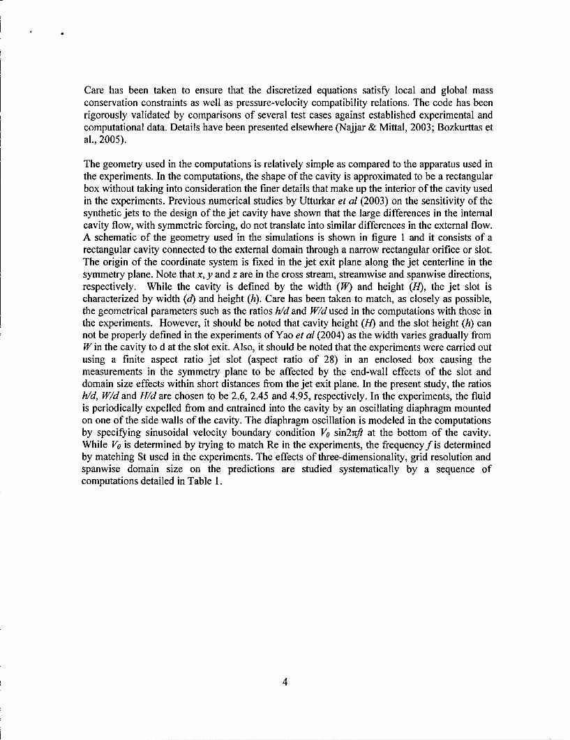
(a) Experimental Setup (b) Computational domain

Figure 1: Schematic of the geometry.

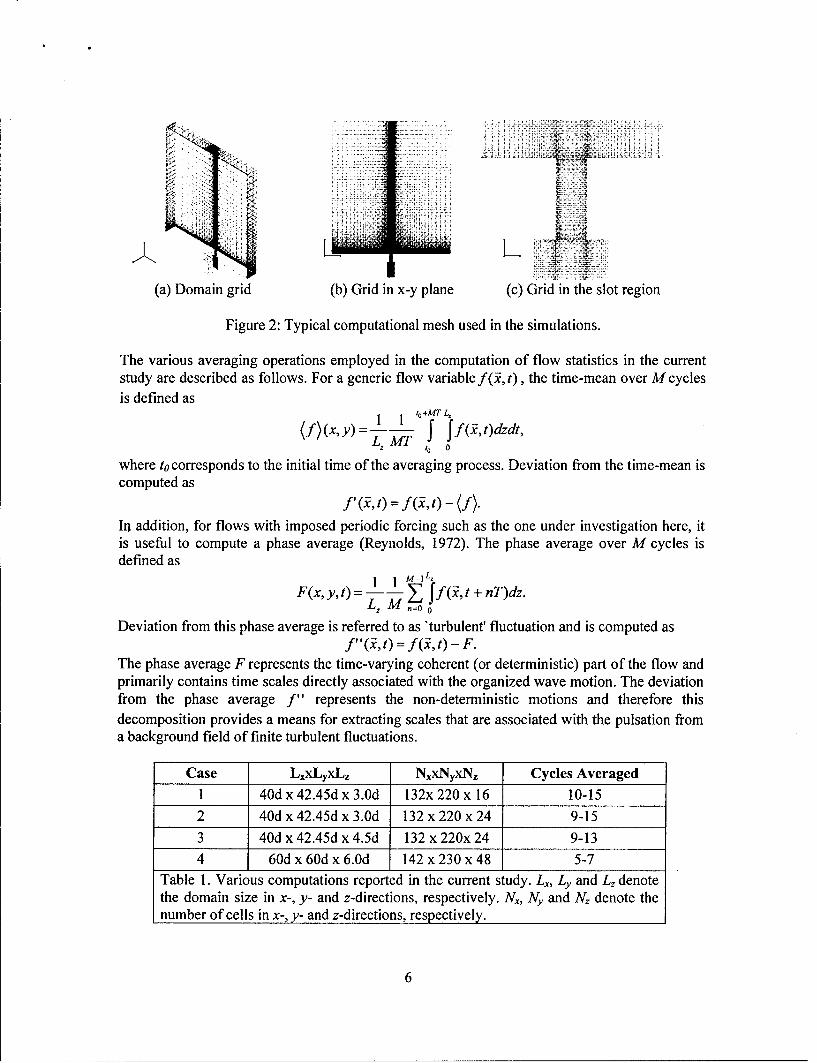
Figure I shows the boundary conditions used in the computations. An outflow velocity boundarycondition is prescribed on the east, west and north boundaries to allow them to respond freely tothe flow created by the jet, and periodic boundary conditions are prescribed in the spanwise (z)direction. The periodicity in the span is intended to model the spanwise homogeneous flowthrough a slot with an infinite spanwise extent. Figures 2a and 2b show, respectively, the domainmesh and an x-y slice of a typical three-dimensional mesh used in the slot region in thecomputations. Grids used in the current work are non-uniform in both x- and y-directions, anduniform in the spanwise (z) direction. Sufficient clustering is provided in the slot-region (figure2c) along x- and y-directions to resolve the vortex structures that form at the slot exit, as well asthe shear layer in the slot. Typically 32x55 grid points are used across the slot. A time stepcorresponding to 14,000 steps per cycle is employed in the calculations. The computations areperformed on a single 2.8 GHz Pentiume 4 processor-based workstation and the CPU timeincurred for Case 4 was around 270 hours per cycle. The three-dimensionality in the solution isinstigated by introducing a small sinusoidal spatial perturbation in the w-velocity over a fewhundred time-steps in the first cycle, and thereafter the three-dimensionality is allowed todevelop on its own through the inherent instability of the flow. The solution was allowed toevolve for several cycles to eliminate transient effects, and only the later cycles detailed in Table1 were used in the computation of flow statistics defined below.

5

Nf

(a) Domain grid (b) Grid in x-y plane (c) Grid in the slot region

Figure 2: Typical computational mesh used in the simulations.

The various averaging operations employed in the computation of flow statistics in the currentstudy are described as follows. For a generic flow variable f(,, t), the time-mean over M cyclesis defined as

(f)(xy) f 1 f+ ,t)dzdt,L, MT 1o o

where to corresponds to the initial time of the averaging process. Deviation from the time-mean iscomputed as

f'(3E, t) = f (-, t) -f.

In addition, for flows with imposed periodic forcing such as the one under investigation here, itis useful to compute a phase average (Reynolds, 1972). The phase average over M cycles isdefined as

-1 Lz

F(x,yt)- -0 f(i, t + nT)dz.L, M n=o0

Deviation from this phase average is referred to as 'turbulent' fluctuation and is computed asf " (5, t) = f(i, t) - F.

The phase average F represents the time-varying coherent (or deterministic) part of the flow andprimarily contains time scales directly associated with the organized wave motion. The deviationfrom the phase average f " represents the non-deterministic motions and therefore thisdecomposition provides a means for extracting scales that are associated with the pulsation froma background field of finite turbulent fluctuations.

Case LxxLyxLz NxxNyxNz Cycles Averaged

1 40d x 42.45d x 3.Od 132x 220 x 16 10-152 40d x 42.45d x 3.Od 132 x 220 x 24 9-153 40d x 42.45d x 4.5d 132 x 220x 24 9-134 60d x 60d x 6.Od 142 x 230 x 48 5-7

Table 1. Various computations reported in the current study. L•, Ly and L, denotethe domain size in x-, y- and z-directions, respectively. N,, Ny and N, denote thenumber of cells in x-, y- and z-directions, respectively.

6

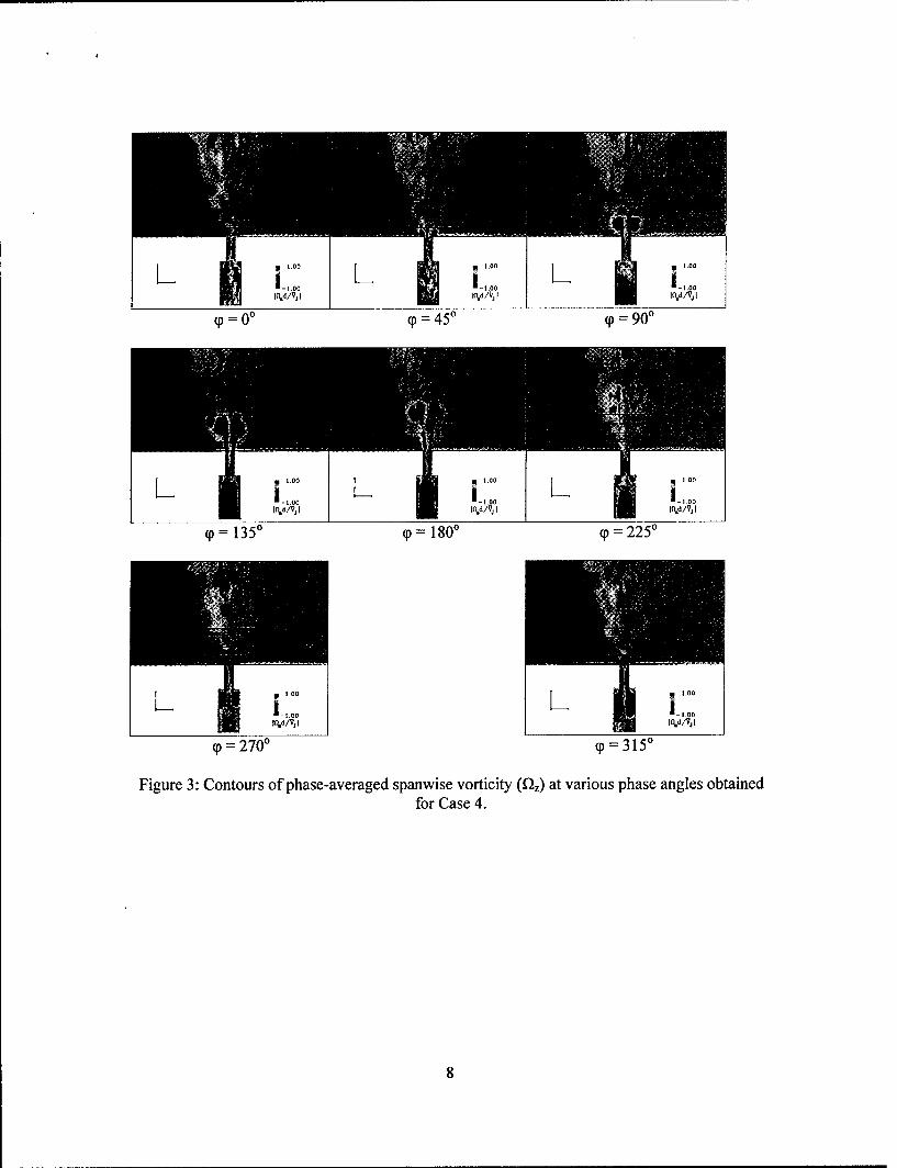
Contours of phase-averaged spanwise vorticity (D,.) obtained for Case 4 are plotted in figure 3 asa function of phase angle T for every 45'. Phase angle p = 0' is arbitrarily chosen to correspondto the commencement of the upward motion of the diaphragm modeled here by the pulsatilevelocity boundary condition at the bottom of the cavity. The horizontal lines seen in thebackground above the jet exit plane are separated from each other and from the slot exit bydistance d. At p = 00, the plot shows some remnants of the previous vortex pair in the near-fieldand the separation of the shear layer in the interior of the slot caused by the suction of theambient fluid into the cavity before the upward motion of the diaphragm began. The plot alsoshows the presence of corner vortices in the cavity. At 450 in phase, a new vortex pair rolls up atthe edges of the slot and its size is of the order of the slot width. The plot also shows separationof the shear layer at the inner edges of the slot. When the rollup process is completed at themaximum-expulsion phase of 900, the vortex pair detaches from the exit plane and grows in sizeas it advects downstream. At p = 135', small-scale structures begin to appear on the rim ofvortex pairs. Also, the rollup of the shear layer at the inner lip of the slot advects downstreamleading to Kelvin-Helmholtz-type instabilities that mark the first stage in the transition process.The expulsion phase is completed and the ingestion phase is commenced at (T = 1800, by whichtime the vortex pair has advected sufficiently downstream (y/d Z 4) that it is not affected by thesuction of ambient fluid into the cavity. At this juncture, the vortex pair loses coherence andbegins to mix with the ambient fluid. At T (- 2250, the vortices lose their individual identity, andthe suction generates vortex rollup in the interior of the cavity. At maximum-ingestion phase of2700, the mixing of the primary vortex pair is complete, resulting in a fully developed turbulentjet beyond y/d = 3. The vortex pair inside the cavity as seen at ip = 3150 starts to grow in sizewhile it descends and engulfs the cavity before the next cycle is begun.

Figure 4 depicts a sequence of plots of isosurfaces of vorticity magnitude obtained for Case 4during the seventh cycle for every 45' in phase. The figure clearly depicts the process oftransition of the primary vortex pair into a fully developed turbulent jet. At the maximum-expulsion phase of 900, the plot shows the presence of spanwise-periodic counter-rotating rib-like vortical structures in the streamwise direction. These streamwise rollers coil around thecores of the primary vortex pair. As the primary vortex pair advects downstream in thesubsequent phases, these spanwise instabilities undergo rapid amplification leading tobreakdown of the primary vortex pair due to three-dimensional vortex stretching and completemixing of the vortices with the ambient fluid within a short distance from the orifice. Thisprocess of transition is consistent with the phase-locked smoke visualizations of a synthetic jet atRe = 766 by Smith and Glezer (1998a).

7

1.00-1.00I_,o L1,,.o0o L'." .

, I•,/v~tiO, /Vj tod/Vji

(P 00 450 cp=900

J100 J 100 V

1.0-1.00 -100Ichd/Vt t~avjI td/VjI

=13 50 (P 1800 p= 2 2 50

%qd/Vt Io ý/V, I

=2 700 p= 3 15 '

Figure 3: Contours of phase-averaged spanwise vorticity (Dz) at various phase angles obtainedfor Case 4.

8

200 ' 200 2,00

900 ==450 9=900

200 2.00

2 0 - 2 .0 0,, /Va I v/A

S27009 = 3150

Figure 5: Isosurfaces of instantaneous vorticity magnitude colored by v-velocity at various phaseangles obtained for Case 4 during the seventh cycle.

Plot of phase-averaged time history of v-velocity obtained from the computations along thevertical centerline at y/d = 0.1 is shown in figure 5. Also included in this plot are the PIV and theLDV measurements of Yao et al (2004). Whereas the computed results show grid convergence,the PIV and LDV measurements show differences amongst themselves with respect to the peakamplitudes and alignment in phase. Even though the PIV data align with the computations atmaximum-ingestion phase (9 = 2700), the maximum-expulsion in the PIV measurements leadsthe computational results by as much as 140 in phase. Nevertheless, in the comparisons of crossstream distributions of various velocity profiles, the results from the simulations at maximum-

9

expulsion phase are validated against the PIV data at p = 90' rather than at p 760 as theagreement is better at p = 900 (not shown here) than at ( = 760.

y/d = 0.1 1CaseCase 2Case 3

- Case 4SPIV. y/d 0.1

0a LDV. y/d =0.08

1 0

00

-1

0 90 180 270 360Phase angle ý, degrees

Figure 5: Plot of phase-averaged v-velocity along the vertical centerline at y/d= 0.1.

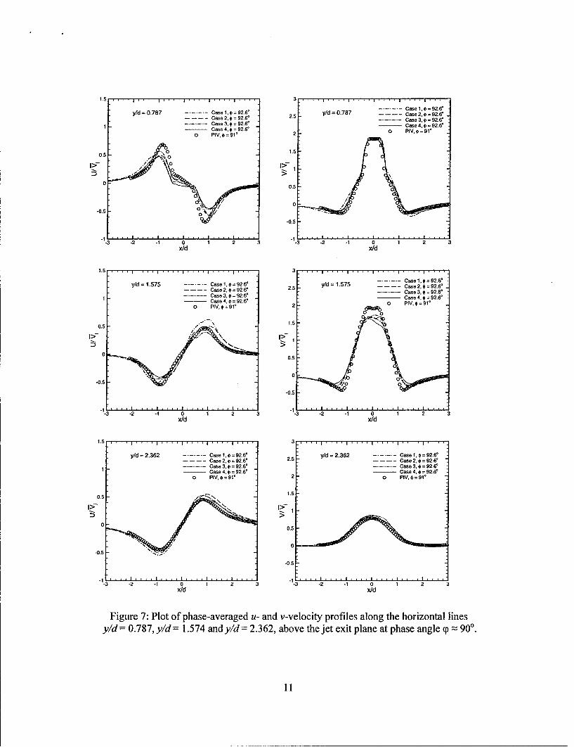
Figure 6 shows the plots of phase-averaged v-velocity profile along the centerlinex/d = 0.0 above the jet exit plane at phase angles 9 z 90' and p = 2700. At the maximum-expulsion phase (( p 900), the computed velocity profiles closely agree with the measurementsfor y/d > 2, and for y/d < 2 the magnitude of the maximum centerline velocity in thecomputations takes a slightly lower value than the measurements. This difference can beattributed to the end wall effects in the experiments that cause the fluid to accelerate betweenshear layers formed at the slot end walls. At the maximum-ingestion phase, results from thecomputations match the measurements until up toy/d = 4 beyond which the computations show higher velocity magnitude than the measurements.Figure 7 shows the comparisons with the measurements of the cross stream distributions ofphase-averaged u- and v-velocity profiles above the jet exit plane at y/d= 0.787, 1.575 and 2.362at p z 900 .

7 . III 17

xld = 0.0xld=O0.0 Case 1, #= 92.6°-. .. Case 1, •= 272.6 i/6Case 2, •= 92.6° 6 Case 2, •= 272.6= / .

Case 3,$= 92.6° -..-..-..-.. Case 3,•= 272.6° /Case 4,#= 92.6° Case 4, •= 272.6°S0 PlV, •= 91 Q PIV, •= 271 =

C4

3 3

2 00 2

0 0.6 I .... 1.5 2 2.5 -2 -1.5 -1 -0.5 0 0.5 1wv/vv.

Figure 6: Plot of phase-averaged v-velocity profile along the vertical centerline x/d=-.0 above thejet exit plane at phase angles (p 900 and (p 2700.

10

S....... Case 1,€ 92.6°

y/d = 0.787 - -. - --- Case 1 ,.ý = 92.6 ° y/d = 0.787 . . . .Case 2, 1 = 92.6*Case 2,0 = 92.6' 2.5 . . .. Case 3, = 92.6'

..... Case 3, 0 = 92.6° __ Case 4, = 92.6°_Case 4, _92Ca0 4, 4 = 92.6'

0 PIV,4 =91 ° 2 0 PIV, 0 91*

\0 1.50.50

00.

0.5

' 0-00

-0.5

.3 -2 ... 1 .. 0 I .. 1 . .2I.....3, I, tI, =,, -2 -1 0 1 2 ... 3

x/d x/d

S....... Case 1. = 92.6'y/d =1.575 ------- Case 1, 0 = 92.6* y/d =1.575 Case 2, 0 = 92.6'

Case 2, 0 = 92.6" 2.5 - ..-..-..- . Case 3, 0 = 92.6 °----------.Case 3. , = 92.6' Case 4, 0 = 92.6'

- Case 4, = 92.6° C 0 ,4, 0 9260 PIV,4 =91° 2 0 PIV,e l=91l

05-1.5I• \I>-

0°.5

00.5

0.

-0.5

x/d x/d

1.5 3

y/d =2.362 ------- Case 1 , 0 = 92.6' y/d =2.362 ------- Case I, 0 = 92.6*

S. . . .- C a se 2 , 0 = 9 2 .6 ' 2 .5 C ase 2 , = 92 .6'

-.-.-.---- Case 3, = 92.6 -..-..--.-- Case 3, = 92.6 °1_- - Case 4, = 92.6 ° Case 4, = 92.6'

o PIV,* =91' 2 o0 PIV.,=91*

0.5 -1.5

I>->

0 0.5

-0.5

-0.5

"1-3 . .-2 I ... 1 .. 0 I .. 1 .. 2 !.. 3 "1.3, ... 2 I ... 1 .. 0 1 .. II.. 2 3 ..

x/d x/d

Figure 7: Plot of phase-averaged u- and v-velocity profiles along the horizontal lines

y/d= 0.787, y`/d= 1.574 andy/d= 2.362, above the jet exit plane at phase angle p = 900.

11

S....... Case 1, =272.6* ....... Case 1, =272.6*y/d= 0.787 Case 2, =272.6* y/d =0.787 ---- Case2, =272.6'

0.4 ......... Case 3, = 272.6 ....... Case3,#=272.6°.••0 PCaV,4 72 0 IV¢ 21

Case 4, =272.6° 0.2 Case 4, € = 272.6°o PIV, p= 271' 0 PIV, ,271*

0.2

0

I>o

.0.2

-0.2

.- 0.4

-0.4

-0.6 . '. .. 1 1 2 3 .0=3-6 '' 1-3 -2 -1 0 1 2 -1 0 1 2 3

x/d x/d

0.6 ... I .. .. .. ...... 0.4 1 1 1 1 . . I . I .

-------. Case 1. =272.6 ....... Case 1, 0 = 272.6°y/d = 1.575 Case 2.0 272.6o yd .1.575 Case 2, = 272.6'

0.4 -..-..-... Case 3,= 272.6W ---... Case 3, t = 272.6'__ Case4, ,=272.6° 0.2 Case 4,* = 272.6°

o PIV, =271* 0 PIV,t=271f

0.2

0-

0 .02

-0.2-

-0.40-0.-

-0.4 06 L..

-0.3 -2 0 1 2 3 3 .2 0 2

x/d x/d

------. Case 1, = 272.6* ------- Case 1, = 272.6"y/d =2.362 Case 2, = 272.6 y/d =2.362 Case 2, = 272.6'

0.4 Case 3, =272.6" . .... Case 3. t = 272.6*Case 4. € = 272.6* 0.2 Case 4, 0 = 272.6*

o PIV,271 271

0.2-0

0 0

0-7-

-0.2

-0.4

-0._6 . . . . -L . . . . -1 . . , a . . ! , i ,2 .. -0.63-21 .2- 3 - 1 0 1 2 3

x/d x/d

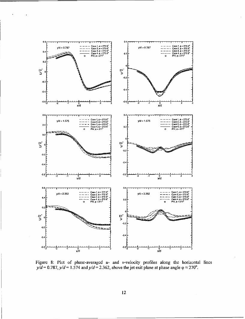
Figure 8: Plot of phase-averaged u- and v-velocity profiles along the horizontal linesy/d = 0.787, y/d = 1.574 and y/d = 2.362, above the jet exit plane at phase angle p ý 2700.

12

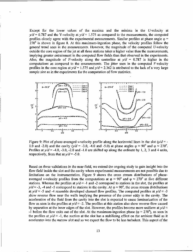
Except for the lower values of the maxima and the minima in the U-velocity aty/d = 0.787 and the V-velocity at y/d = 1.575 as compared to the measurements, the computedprofiles closely agree with the experimental measurements. Similar profiles at phase angle (p =

2700 is shown in figure 8. At this maximum-ingestion phase, the velocity profiles follow thegeneral trend seen in the measurements. However, the magnitude of the computed U-velocityoutside the core region of the jet at all three stations takes a higher value than the measurements,implying greater entrainment in the computed flow fields than that observed in the experiments.Also, the magnitude of V-velocity along the centerline at y/d = 0.787 is higher in thecomputations as compared to the measurements. The jitter seen in the computed V-velocityprofiles in the core region at y/d = 1.575 and y/d = 2.362 is attributed to the lack of a very largesample size as in the experiments for the computation of flow statistics.

*=92.6* J Case2 ,=272.6' ---- Case2---- -Case3 ---- -Case 3

5Yld-2.0 Case 4" Case 4 y/d -1.0

4 3y/d=-2.0

-32* Y/d=-3.0-

2

i y/d = -4.0

y/d = -5.0 "5

-0.5 0 0.5 1 -1 -0.5 0 0.5 1x/d x/d

Figure 9: Plot of phase-averaged v-velocity profile along the horizontal lines in the slot (y/d -

1.0 and -2.0) and the cavity (y/d = -3.0, -4.0 and -5.0) at phase angles :5 90' and T : 2700.Profiles at y/d = -4.0, -3.0, -2.0 and -1.0 are shifted up along the ordinate by 1, 2, 3 and 4 units,respectively, from that aty/d= -5.0.

Based on these validations in the near-field, we extend the ongoing study to gain insight into theflow field inside the slot and the cavity where experimental measurements are not possible due tolimitations on the instrumentation. Figure 9 shows the cross stream distributions of phase-averaged v-velocity profiles from the computations at T 'z 90' and 9 p 2700 at five differentstations. Whereas the profiles at y/d = -l and -2 correspond to stations in the slot, the profiles aty/d z -3, -4 and -5 correspond to stations in the cavity. At y = 900, the cross stream distributionsat y/d - -5 and -4 resemble developed channel flow profiles. The computed profiles at y/d = -3show reverse flow near the walls implying the presence of the comer eddy in the cavity. Theacceleration of the fluid from the cavity into the slot is expected to cause laminarization of theflow as seen in the profiles at y/d z -2. The profiles at this station also show reverse flow causedby separation at the inner edges of the slot. However, the profiles become more uniform at y/d-1 before the flow exits out of the slot. At the maximum-ingestion phase (p = 2700), as seen inthe profiles at y/d z -1, the suction at the slot has a stabilizing effect on the ambient fluid as itaccelerates into the narrow slot and so we expect the flow to be less turbulent. This aspect of the

13

flow is looked at in more detail using spectral analysis discussed later. However, the flowrecovers the developed profile at y/d z -2 before it exits out of the slot and rolls up into a vortexpair in the cavity. Profiles at y/d 2 -3 and -4 show recirculation regions characterized by thevortex pair in the cavity. At y/d = -5, the profiles do not show any flow reversals as this station isnot within the reach of the vortex pair at this instant in phase.

6 ------- Case 1Case 2 .

____ Case 45 o PIV

4

37

2

0 0.2 0.4 0.6 0.8 1

<v>/ V

Figure 10: Plot of time-averaged v-velocity profile along the vertical centerline x/d= 0.0 abovethe jet exit plane.

Figure 10 shows the comparisons of the computed time-averaged v-velocity profiles with theexperiments along the vertical centerline above the jet exit plane. The plot shows consistentlylower values in the computed profiles as compared to the measurements. The cross streamdistributions of the time-averaged u- and v-velocity profiles are shown in figure 11 at threestations (y/d = 0.787, 1.575 and 2.362) above the jet exit plane. While the computed <u>-velocity profiles consistently show higher values than the measurements outside the core regionof the jet at all stations, the computed <v>-velocity profiles closely match the experimentsexcept for the lower values along the jet centerline as compared to the measurements. Time-averaged v-velocity profiles at five stations in the slot and the cavity are shown in figure 12. It isinteresting to note that while the velocity in the shear layer at y/d = -1 is positive, the velocity isnegative in the shear layer at y/d --2 implying that somewhere in between these two stations, themean cross stream distribution is zero across the slot since the net mass flux is zero. In thecavity, <v>-velocity is positive in the shear layer at all three stations, whereas it is negative in thecore

14

0.4 I. . I ' I 0.6 - - - ý

------- Case Iy/d =0.787 Case2 y/d= 0.787 ------- Case 1

0.3 ...... Case3- -.. .Case2ase4 o .... .Case3.2Case4 -0 Case40 PIV 0.4 0 o PIV

0.4- 0. iP>-0.2 0

I>;- 0.17A 0. 2

V0-

-0.1

00.

-0.2 -0 I

-3 -2 -1 0 1 2 3 -3 -2 -1 0 1 2 3x/d x/d

0.4 0.6

y/d =1.575 ------- Case I y/d =1.575 01ob ------- Case I

0.3 Case2 o Case2--------. Case 3 . .Case 3

-- Case 4 _ _ i Case 4o PIV 0.4 0 PIV

0.2

I>- 0.1 7 7

"V 00

-0.1N0

7o_

-0.2

.0 .3.3 . . . . .. . . .1 .. .. . .. .. . . . . .- . . . I . . . . I . . . . ! . .-3 2 -1 0 1 2 3-02- -2 -1 0 2 3

x/d x/d

0.4 . . . . . . . . . . . 0.6 , j . . . .

y/d 2.362 ------- Case 1 y/d =2.362 ----.-- Case I0.3 7 Case2 0 Case2.--------- Case 3 .. o ...... Case 3

- Case 4 ______ Case 40 PiV 0.4 0 PIV

0.2

7ooA ~0.2

V 0

-0.10

-0.2

.0 "3-3 .. . 2 I .. . JO* 1.. 0! . . . . 2 ! . . 0 -3 . .. -2 ! .. -1 . . 0 i . . 1 . . 2 I . . 3

x/d /d

Figure 11: Plot of time-averaged u- and v-velocity profiles along the horizontal linesy/d = 0.787, y/d= 1.574 andy/d = 2.362, above thejet exit plane.

15

-.----- Case 1Case 25 ....----- Case 3Case 4

4 -l

y/d =-2.03> - Vo", N

A S2 f - " "-'- • ~y~d =-3 0 - - -- -

0 -• y/d = -4.0

-1 -0.S 0 0.S 1

x/d

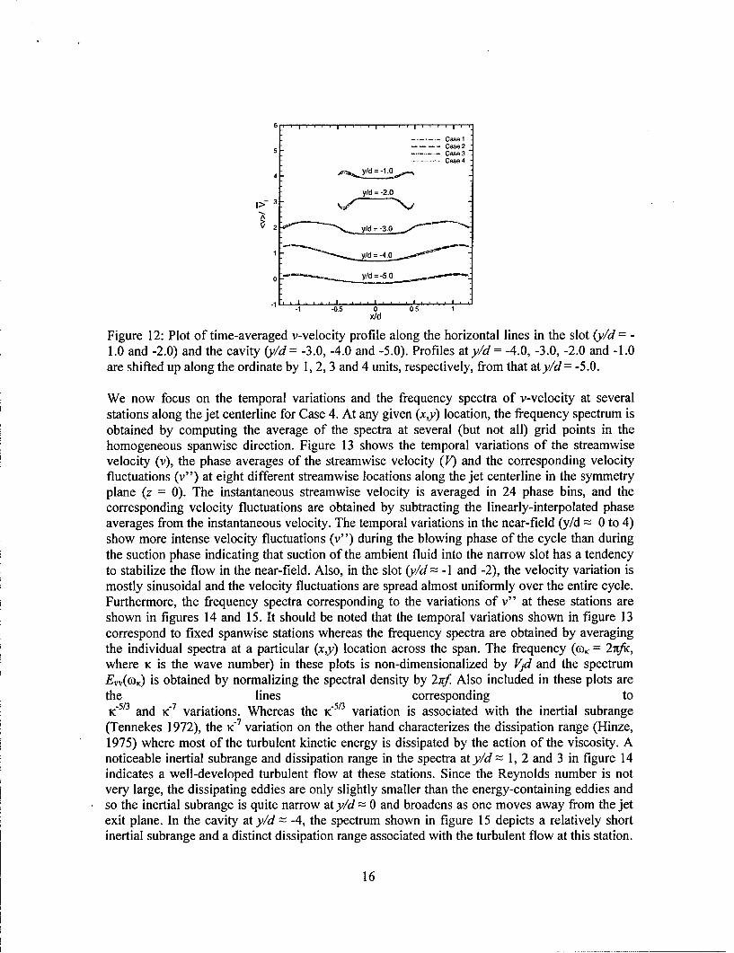
Figure 12: Plot of time-averaged v-velocity profile along the horizontal lines in the slot (y/d -

1.0 and -2.0) and the cavity (y/d = -3.0, -4.0 and -5.0). Profiles at y/d = -4.0, -3.0, -2.0 and -1.0are shifted up along the ordinate by 1, 2, 3 and 4 units, respectively, from that aty/d= -5.0.

We now focus on the temporal variations and the frequency spectra of v-velocity at severalstations along the jet centerline for Case 4. At any given (xy) location, the frequency spectrum isobtained by computing the average of the spectra at several (but not all) grid points in thehomogeneous spanwise direction. Figure 13 shows the temporal variations of the streamwisevelocity (v), the phase averages of the streamwise velocity (P) and the corresponding velocityfluctuations (v") at eight different streamwise locations along the jet centerline in the symmetryplane (z = 0). The instantaneous streamwise velocity is averaged in 24 phase bins, and thecorresponding velocity fluctuations are obtained by subtracting the linearly-interpolated phaseaverages from the instantaneous velocity. The temporal variations in the near-field (y/d- 0 to 4)show more intense velocity fluctuations (v") during the blowing phase of the cycle than duringthe suction phase indicating that suction of the ambient fluid into the narrow slot has a tendencyto stabilize the flow in the near-field. Also, in the slot (y/d -1 and -2), the velocity variation ismostly sinusoidal and the velocity fluctuations are spread almost uniformly over the entire cycle.Furthermore, the frequency spectra corresponding to the variations of v" at these stations areshown in figures 14 and 15. It should be noted that the temporal variations shown in figure 13correspond to fixed spanwise stations whereas the frequency spectra are obtained by averagingthe individual spectra at a particular (xy) location across the span. The frequency (co, = 27ific,where K is the wave number) in these plots is non-dimensionalized by V.d and the spectrumEVV(coK) is obtained by normalizing the spectral density by 27.f Also included in these plots arethe lines corresponding toK"513 and K-7 variations. Whereas the k-513 variation is associated with the inertial subrange(Tennekes 1972), the K 7 variation on the other hand characterizes the dissipation range (Hinze,1975) where most of the turbulent kinetic energy is dissipated by the action of the viscosity. Anoticeable inertial subrange and dissipation range in the spectra at y/d = 1, 2 and 3 in figure 14indicates a well-developed turbulent flow at these stations. Since the Reynolds number is notvery large, the dissipating eddies are only slightly smaller than the energy-containing eddies andso the inertial subrange is quite narrow at y/d : 0 and broadens as one moves away from the jetexit plane. In the cavity at y/d = -4, the spectrum shown in figure 15 depicts a relatively shortinertial subrange and a distinct dissipation range associated with the turbulent flow at this station.

16

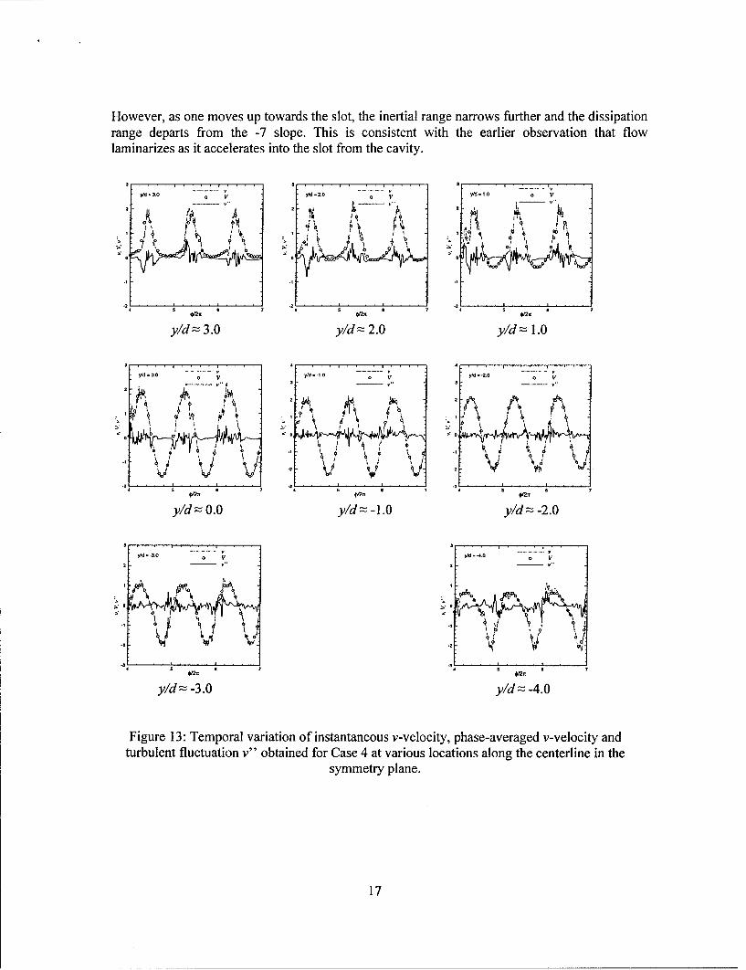
However, as one moves up towards the slot, the inertial range narrows further and the dissipationrange departs from the -7 slope. This is consistent with the earlier observation that flowlaminarizes as it accelerates into the slot from the cavity.

I .. . I ' '~ ... L _ . . . . . I . . .,.. . . . .. . . . .. , .......... I - -

yd-3,0 o V y.O = 2.0 0 v y79 - 1.0 0 V

V 0

2 . '. . .. . . . . . .4 5 7 4 , 4 1

iity/d 3.0 y/d 2.0 y/d 1.0

y/d 0.0 0 V y/d--,4. vo V

2 37 3- .

77

V V VVy/d -0 y/d 10 y/dz; -2.0

y/d.3 - D yld--400

-2 --2 AV

.3 L

02 V 2.

y/dz -3.0 y/d z -4. 0

Figure 13: Temporal variation of instantaneous v-velocity, phase-averaged v-velocity andturbulent fluctuation v" obtained for Case 4 at various locations along the centerline in the

symmetry plane.

17

10'

102

"(y"d2..0)\\10 -

S(y/d=].O)

102 _

(y/d= 0. 0) .

10'

10", Case 4 ' ,

10 1 . .. ..

10" 100 10wDd/ Vj

Figure 14: Frequency spectra corresponding to turbulent fluctuations v" along the centerline aty/dz 0.0, 1.0, 2.0 and 3.0 for Case 4. Note that the spectrum aty/d- 1.0, 2.0 and 3.0 is shifted upby two, four and six decades, respectively, from that at y/d 0.0. Dash-dot-dot and dashed linescorrespond to K-5 /3 and k-7 variations, respectively.

.- N \ \ N

10.

100 (/d 2) A-.,..

100s

10.2\ "

(y/d -4.0)

10 10

0) d/V.

Figure 15: Frequency spectra corresponding to turbulent fluctuations v" along the centerline aty/d =-1.0, -2.0, -3.0 and -4.0 for Case 4. Note that the spectrum at y/d =-3.0, -2.0 and -1.0 isshifted up by two, four and six decades, respectively, from that aty/d = -4.0. Dash-dot-dot and dashed lines correspond to K-51 3 and K< variations, respectively.

18

b. Low Dimensional Modeling of ZNMF Actuators

Ongoing experimental and computational studies are focused on ZNMF actuators in bothquiescent and grazing flows; however numerous unresolved issues remain concerning thefundamental governing physics of these devices, effectively hindering their modeling, design andoptimization. For example, the unsteady flow in the orifice or slot plays a large role indetermining the actuator performance. While numerous parametric studies have examinedvarious orifice geometry and flow conditions, a clear understanding of the loss mechanisms isstill lacking. Detailed numerical simulations (and companion experiments) can be used toelucidate the underlying physics but are not practical as a design tool. Instead, accurate lowdimensional models are required to facilitate the effective design of ZNMF actuators for specificapplications. While the ultimate goal is to develop models suitable for use in boundary layer flowcontrol in which the ZNMF actuator interacts with a grazing flow, the ongoing collaborativeeffort focuses on experimental and computational efforts to first understand and model theoscillatory orifice flow in the simpler case without a grazing flow. In particular, experimentaldata and numerical simulations are used to explore the flow behavior and develop componentsfor a low-order lumped element model of more commonly employed sharp-edged orifice or slotof a ZNMF actuator. The effects of various governing dimensionless parameters are examined.

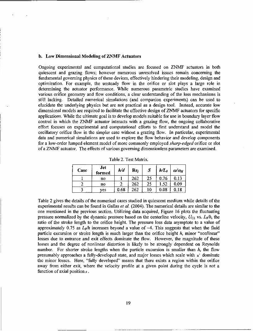
Table 2. Test Matrix.

Case JetCase_ formed h/d Re, S hiLo W0H

1 no 1 262 25 0.76 0.132 no 2 262 25 1.52 0.093 yes 0.68 262 10 0.08 0.18

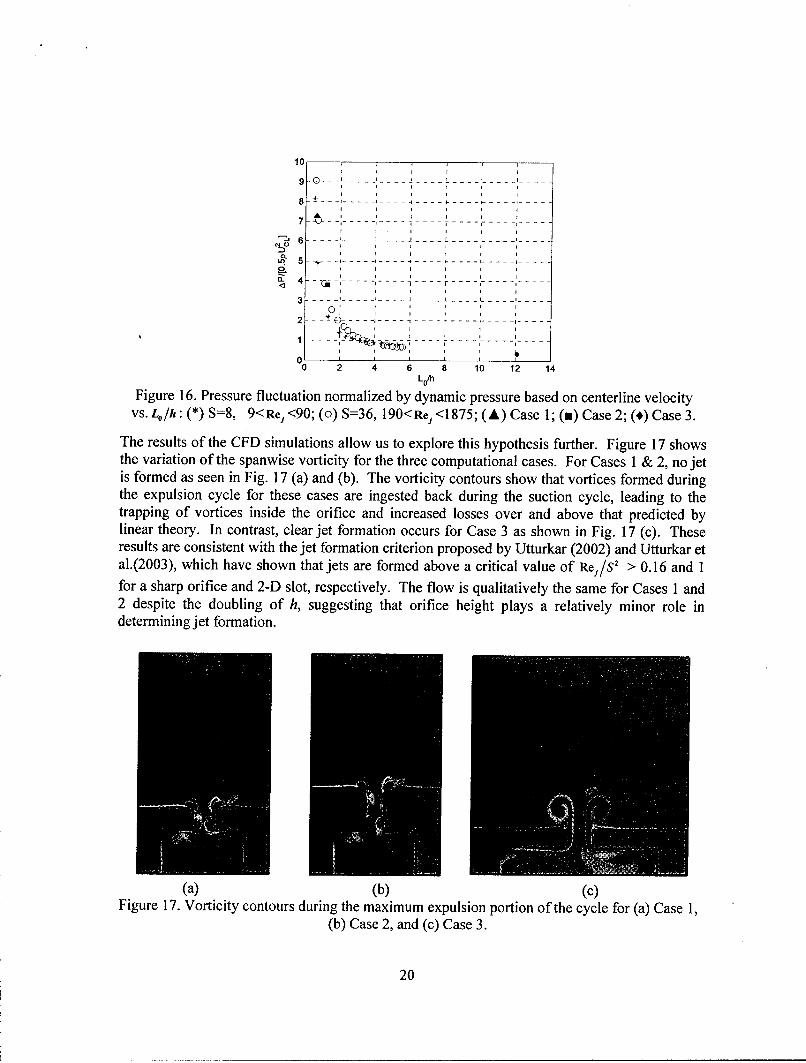
Table 2 gives the details of the numerical cases studied in quiescent medium while details of theexperimental results can be found in Gallas et al. (2004). The numerical details are similar to theone mentioned in the previous section. Utilizing data acquired, Figure 16 plots the fluctuatingpressure normalized by the dynamic pressure based on the centerline velocity, UcL vs. Lo/h, theratio of the stroke length to the orifice height. The pressure loss data asymptote to a value ofapproximately 0.75 as Lo/h increases beyond a value of -4. This suggests that when the fluidparticle excursion or stroke length is much larger than the orifice height h, minor "nonlinear"losses due to entrance and exit effects dominate the flow. However, the magnitude of theselosses and the degree of nonlinear distortion is likely to be strongly dependent on Reynoldsnumber. For shorter stroke lengths when the particle excursion is smaller than h, the flowpresumably approaches a fully-developed state, and major losses which scale with u' dominatethe minor losses. Here, "fully developed" means that there exists a region within the orificeaway from either exit, where the velocity profile at a given point during the cycle is not afunction of axial position x.

19

10

9 -- -- - ----- - - -

I I I I I I

7 - ---- - -. .- --- - . .- - . . .-- - -- -- . . . - - - - -- -- --

7 - - -'- -

'a 5 - --+I---------- --

3 - - - I26 ,' - - ,

2 , l I I I

3 1 - -

010 2 4 6 8 10 12 14

Lo/h

Figure 16. Pressure fluctuation normalized by dynamic pressure based on centerline velocityvs. Lo/h: (*) S=8, 9<Re, <90; (o) S=36, 190<Re, <1875; (A) Case 1; (a) Case 2; (*) Case 3.

The results of the CFD simulations allow us to explore this hypothesis further. Figure 17 showsthe variation of the spanwise vorticity for the three computational cases. For Cases 1 & 2, no jetis formed as seen in Fig. 17 (a) and (b). The vorticity contours show that vortices formed duringthe expulsion cycle for these cases are ingested back during the suction cycle, leading to thetrapping of vortices inside the orifice and increased losses over and above that predicted bylinear theory. In contrast, clear jet formation occurs for Case 3 as shown in Fig. 17 (c). Theseresults are consistent with the jet formation criterion proposed by Utturkar (2002) and Utturkar etal.(2003), which have shown that jets are formed above a critical value of Re,/S 2 > 0.16 and 1for a sharp orifice and 2-D slot, respectively. The flow is qualitatively the same for Cases 1 and2 despite the doubling of h, suggesting that orifice height plays a relatively minor role indetermining jet formation.

(a) (b) (c)Figure 17. Vorticity contours during the maximum expulsion portion of the cycle for (a) Case 1,

(b) Case 2, and (c) Case 3.

20

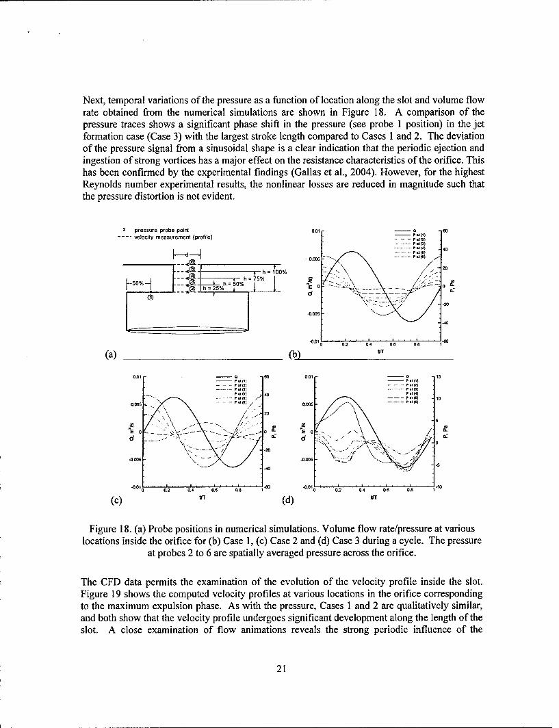
Next, temporal variations of the pressure as a function of location along the slot and volume flowrate obtained from the numerical simulations are shown in Figure 18. A comparison of thepressure traces shows a significant phase shift in the pressure (see probe 1 position) in the jetformation case (Case 3) with the largest stroke length compared to Cases 1 and 2. The deviationof the pressure signal from a sinusoidal shape is a clear indication that the periodic ejection andingestion of strong vortices has a major effect on the resistance characteristics of the orifice. Thishas been confirmed by the experimental findings (Gallas et al., 2004). However, for the highestReynolds number experimental results, the nonlinear losses are reduced in magnitude such thatthe pressure distortion is not evident.

x pressure probe point Q.01 - a. velocity measurement (profile) p M()

-- W- - (2)P =t (3)' "t 0; 40P , t(10005 ....... ",M r)//

ii~ h~OO% /20t h= 100%

ih=25% a:.. .

S- / -20

-0.011 . . . . . . A -60

0 0.2 0.4 0.6 oe.

(a) (b) UT

0.01 - -- o0 0.01 - - 15P SItll ____ P efltl- P-- 521 - P Mf

P .t (3] p itI

P .1(1 Y; P40t 10

aO00 - -• P* ) o 0.00P

20

I.-L.•. .r.=•< o •- 0: / 0

K d00" !.. v_- . 0s- -.•

•OOD -40D -, A

-0A0.0 . . - -0.010 L-100.2 0.4 0.8 0.0 02 004 002 0.8

(c) UT (d) UT

Figure 18. (a) Probe positions in numerical simulations. Volume flow rate/pressure at variouslocations inside the orifice for (b) Case 1, (c) Case 2 and (d) Case 3 during a cycle. The pressure

at probes 2 to 6 are spatially averaged pressure across the orifice.

The CFD data permits the examination of the evolution of the velocity profile inside the slot.Figure 19 shows the computed velocity profiles at various locations in the orifice correspondingto the maximum expulsion phase. As with the pressure, Cases 1 and 2 are qualitatively similar,and both show that the velocity profile undergoes significant development along the length of theslot. A close examination of flow animations reveals the strong periodic influence of the

21

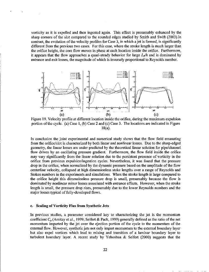
vorticity as it is expelled and then ingested again. This effect is presumably enhanced by thesharp corners of the slot compared to the rounded edges studied by Smith and Swift (2003).Incontrast, the evolution of the velocity profiles for Case 3, in which ajet is formed, is significantlydifferent from the previous two cases. For this case, where the stroke length is much larger thanthe orifice height, the core flow moves in phase at each location inside the orifice. Furthermore,it appears that the flow approaches a quasi-steady behavior for large Lc/h and is dominated byentrance and exit losses, the magnitude of which is inversely proportional to Reynolds number.

3 3-bo5 -

225

2 2

l0,. l 1.5. . .. ........... . ." "- --'0 . ''

01 1T : * 1 .

00 0.

o :25 0.5 0175 It1 . 0 02 0.4 0.6 00. S ... 1 0 5 0t O2 0.4 0.0 GAs I

yfd yld yld

(a) (b) (c)Figure 19. Velocity profile at different location inside the orifice, during the maximum expulsionportion of the cycle. (a) Case 1, (b) Case 2 and (c) Case 3. The locations are indicated in Figure

18(a).

In conclusion the joint experimental and numerical study shows that the flow field emanatingfrom the orifice/slot is characterized by both linear and nonlinear losses. Due to the sharp-edgedgeometry, the linear losses are under predicted by the theoretical linear solution for pipe/channelflow driven by an oscillating pressure gradient. Furthermore, the flow field inside the orificemay vary significantly from the linear solution due to the persistent presence of vorticity in theorifice from previous expulsion/ingestion cycles. Nevertheless, it was found that the pressuredrop in the orifice, when normalized by the dynamic pressure based on the amplitude of the flowcenterline velocity, collapsed at high dimensionless stoke lengths over a range of Reynolds andStokes numbers in the experiments and simulations. When the stroke length is large compared tothe orifice height this dimensionless pressure drop is small, presumably because the flow isdominated by nonlinear minor losses associated with entrance effects. However, when the strokelength is small, the pressure drop rises, presumably due to the lower Reynolds numbers and themajor losses typical of fully-developed flows.

c. Scaling of Vorticity Flus from Synthetic Jets

In previous studies, a parameter considered key to characterizing the jet is the momentumcoefficient C•, (Amitay et al., 1999; Seifert & Pack, 1999) generally defined as the ratio of the netmomentum imparted by the jet over the ejection portion of the cycle to the momentum of theexternal flow. However, synthetic jets not only impart momentum to the external boundary layerbut also expel vortices which lead to mixing and transition of a laminar boundary layer toturbulent boundary layer. A recent study by Yehoshua & Seifert (2000) suggests that the

22

vorticity flux is an important factor for grazing flows. Past simulations and experiments haveshown that the vorticity flux is the key aspect that determines the "formation" of synthetic jets inquiescent flow (Utturkar et al., 2003). This flux of vorticity, f(v during the expulsion can bedefined as,

T/2 d/2Q Ifd12, udydt

0 0

where 4, is the vorticity component of interest and T is the time period.

It would therefore be useful to develop scaling laws for the vorticity flux of ZNMF jets ingrazing flows. Based on previous simulations we propose the following functional dependenceas,

C -fin(St,- ,Re.j

Vj d Vj d

where, 6/d and U.. / V are dependent on the incoming boundary layer.

Here we report some of the preliminary findings for developing this scaling law. 2-Dcomputations have been performed for simplified geometry for ZNMF actuator for fixed cavitywidth (W/D = 3) and slot height (h/d = 1). Functional dependencies are studied by varying oneof the parameters with the others held fixed. Due to the extensive range of the probabilities, wehave chosen relatively low Reynolds number cases for preliminary studies. The range of thesame has been in listed in Table 3.

Table 3. Range of parameters varied

Parameters Range_ _ _d 0.5-3.0

u- /VJ 0.5-4.0

Re1 93.75-500

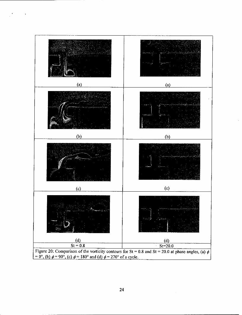
This set of calculations yield a range of Reynolds number based on the boundary layer thickness(Re, = U.1 /v) of 125 - 4000 while for that of Strouhal number, St is found to be 0.1 - 26.7. Itis found that during the expulsion phase the actuator expels vortices which essentially trip theboundary layer in the proximity of the jet. In the process vortices formed are carried furtherdownstream by the interacting boundary layer. Figure 20 shows the vorticity contours of asynthetic jet interacting with the laminar boundary at Re6=1000 for St = 0.8 and 20.0. For St =0.80 (Rej = 125, S = 10) the expelled vortices are swept away by the laminar boundary layer. Forthe same Rej = 125, at significantly high Stokes number (S=20) the vortices formed are notcompletely expelled, and are ingested back as seen in Figure 20. This indicates that forsufficiently high St the vorticity flux might not be having a significant affect on the boundarylayer.

23

(a) (a)

(b) (b)

(c) (c)

(d) (d)St = 0.8 St=20.0

Figure 20: Comparison of the vorticity contours for St = 0.8 and St = 20.0 at phase angles, (a) %6= 0', (b) 0 = 90', (c) 0 = 1800 and (d) 0 = 270' of a cycle.

24

d/2

The normalized instantaneous vorticity flux, Q(t) = f',udy based on the magnitude of vorticity0

across the slot exit, has been shown in Figure 2 1(a) as function of phase for St = 3.2 and U /v =

4. For fixed Rej = 125 and S = 10 (St = 3.2), the time averaged vorticity flux is plotted as afunction of 6/d in Figure 21(b). For very low values of 5/das expected there is a highmagnitude of vorticity which decreases towards to an asymptotic with an increase in theboundary layer thickness. For ,5/d > 2 this variation is marginal indicating that the vortices arenot able to penetrate boundary layer at these values.

20 12

1115

10

10 9 ,

85 6

5.574

-10 3

2-15 ""200 0 ,,,., , I_,_____ _________ ,_____ ,___ ,_,__

0 360 720 1080 1440 0 1 2 3 4

48/d

(a) (b)Figure 21: (a) Normalized Qv(t) across the slot exit as a function of the phase for four cycles, (b)normalized K•v across the slot exit as a function of the varying 8/d.

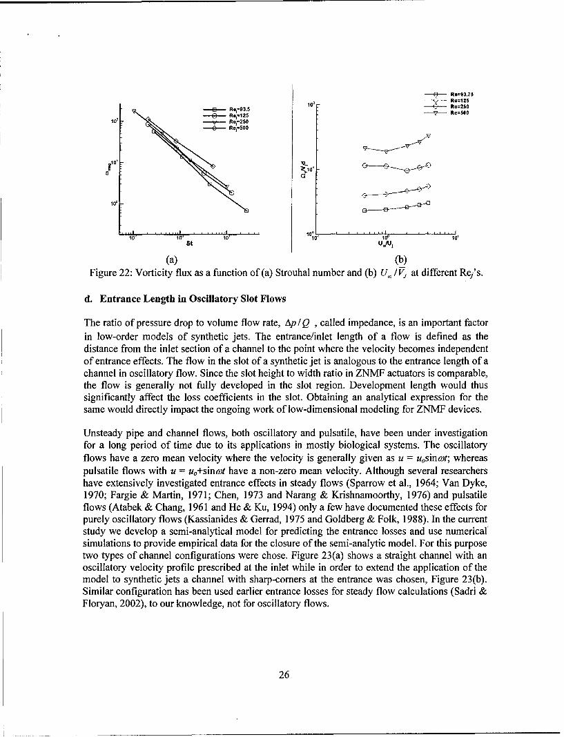
Figure 22(a) shows the variation of the vorticity flux n, with increasing St. Here St has beenvaried from 0.10 to 26.67 for four different Rej's while fixing U, / V, =4. The plot shows analmost a linear behavior of ), with respect to St for all the Reynolds numbers. This is similar tothe experimental findings for quiescent flows. On the other hand the vorticity flux shows a weakdependence on U./ over a range of 0.5 to 4 with the other parameters fixed, seen in Figure

22(b). We are currently analyzing the data for a power law type scaling, -=- 81.St U

where /,,2 and c-are to be determined.

25

-B---R.:93.70

lol- Re=125

1--- Re =93 Re=250

-0- - Re =12510' V Re,=250

E) Re,-500

3 _4

10°0 .

100 10,

St UJUj

(a) (b)Figure 22: Vorticity flux as a function of(a) Strouhal number and (b) U.I /V, at different Rey's.

d. Entrance Length in Oscillatory Slot Flows

The ratio of pressure drop to volume flow rate, ApIQ , called impedance, is an important factorin low-order models of synthetic jets. The entrance/inlet length of a flow is defined as thedistance from the inlet section of a channel to the point where the velocity becomes independentof entrance effects. The flow in the slot of a synthetic jet is analogous to the entrance length of achannel in oscillatory flow. Since the slot height to width ratio in ZNMF actuators is comparable,the flow is generally not fully developed in the slot region. Development length would thussignificantly affect the loss coefficients in the slot. Obtaining an analytical expression for thesame would directly impact the ongoing work of low-dimensional modeling for ZNMF devices.

Unsteady pipe and channel flows, both oscillatory and pulsatile, have been under investigationfor a long period of time due to its applications in mostly biological systems. The oscillatoryflows have a zero mean velocity where the velocity is generally given as u = uosinaot; whereaspulsatile flows with u = uo+sino)t have a non-zero mean velocity. Although several researchershave extensively investigated entrance effects in steady flows (Sparrow et al., 1964; Van Dyke,1970; Fargie & Martin, 1971; Chen, 1973 and Narang & Krishnamoorthy, 1976) and pulsatileflows (Atabek & Chang, 1961 and He & Ku, 1994) only a few have documented these effects forpurely oscillatory flows (Kassianides & Gerrad, 1975 and Goldberg & Folk, 1988). In the currentstudy we develop a semi-analytical model for predicting the entrance losses and use numericalsimulations to provide empirical data for the closure of the semi-analytic model. For this purposetwo types of channel configurations were chose. Figure 23(a) shows a straight channel with anoscillatory velocity profile prescribed at the inlet while in order to extend the application of themodel to synthetic jets a channel with sharp-comers at the entrance was chosen, Figure 23(b).Similar configuration has been used earlier entrance losses for steady flow calculations (Sadri &Floryan, 2002), to our knowledge, not for oscillatory flows.

26

Q(t) =QSinai. -. . a .. ...

(a) LE

1(t) =u.Sinal . ............ .

(b)

Figure 23: Schematic of entrance flow in a (a) straight channel and (b) channel with a sharp-comers.

The governing equations for flow through 2-D channel of height, h with rigid walls as seen inFigure 23(a), can be non-dimensionalized based on the Stokes number, S. Assuming there is nocross-component of the velocity and integrating across a section of the channel the N-S equationscan be simplified in terms of the axial velocity, u as,

S2 aQ a 'd -9j . au_+__ fu~d P

at axl , x 0-

where Q(t) and P are the volumetric flow rate and average pressure across the channel heightrespectively.

We assume a profile of the axial velocity of the following form based on the analytical solutionfor developing laminar steady flow in a channel given by Fargie and Martin (1971),

S( u o ( t ) f o r 0 < _ y < _ c e ( x )

uo(t)f(a,y,S) fora(x)<•y<_l

where, f(a,y,S) = Real cosh(S')- cosh(S'z)- based on the theoretical model given for unsteadywhre fayS)= I cosh(S') - I1

fully-developed flows by Loundon and Tordesillas (1998), uo(t) is the oscillatory velocity, a(x) isthe core length ((1-a) is the boundary layer thickness) , S'= Sli and z=y-all-a.

The continuity equation yields the form of uo(t) based on KI(S) ,a known integral function of Sas,

u4 (Q(t)2(a + (1 - a)K, (s))

27

This yields a final form of the solution for the pressure loss by integrationover the entrance length LE as,

-P s2 = -Q2 K2(S) QK 3 (S')'j

- at 4L(K1 (S))2 2 0o(1-aXa+(I-a)K1 (S))

where K2 and K3 are again known integral functions of S. The first term on the RHS representsthe loss coefficient due to the inviscid acceleration, the second due to entrance loss from theconvective term and the third are due to the viscous effects. Hence we can obtain a closed formexpression for determining the loss coefficients in the entrance length of a channel.

The key unknown for the closed form expression is the core length a(x) which essentially is afunction of the entrance length LE. The entrance length for pulsatile flows is given asLE/h = 2.64/St when an oscillation is superimposed on a steady flow (Fung, 1997). This showsthat the entrance length for these flows is inversely proportional to the Strouhal number. Theobjective here is to develop similar scaling law for a purely oscillatory flow using numericalsimulations, which then would be used to obtain an expression for ax(x).

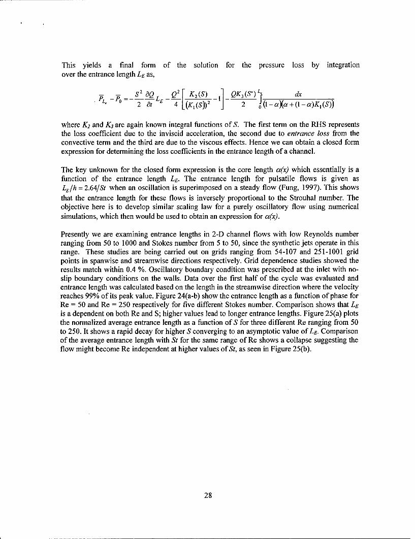
Presently we are examining entrance lengths in 2-D channel flows with low Reynolds numberranging from 50 to 1000 and Stokes number from 5 to 50, since the synthetic jets operate in thisrange. These studies are being carried out on grids ranging from 54-107 and 251-1001 gridpoints in spanwise and streamwise directions respectively. Grid dependence studies showed theresults match within 0.4 %. Oscillatory boundary condition was prescribed at the inlet with no-slip boundary conditions on the walls. Data over the first half of the cycle was evaluated andentrance length was calculated based on the length in the streamwise direction where the velocityreaches 99% of its peak value. Figure 24(a-b) show the entrance length as a function of phase forRe = 50 and Re = 250 respectively for five different Stokes number. Comparison shows that LE

is a dependent on both Re and S; higher values lead to longer entrance lengths. Figure 25(a) plotsthe normalized average entrance length as a function of S for three different Re ranging from 50to 250. It shows a rapid decay for higher S converging to an asymptotic value of LE. Comparisonof the average entrance length with St for the same range of Re shows a collapse suggesting theflow might become Re independent at higher values of St, as seen in Figure 25(b).

28

25-

Ss=1o -w S=-l-a--- SIS -- S=2O

4 ---8--4--- $2 s=3o 0 -x0s3

5-J

2 .10

O .. . .0 .0 120 .50 . .2030 60 0 120 150 1800

20 10

(a) (b)Figure 24: Entrance length variation as a function of phase for varying Stokes number at (a) Re =

50 and (b) Re = 250.

12 10-y-U--R::50 RU-- - 5R00SRe.100 1 R::100

- - R-250 - R. 250

!lop

•"" •\ 0"

00

2 st

0 10 20 30 .10 10' 10S St

(a) (b)Figure 25: Average entrance length as a function of (a) Stokes number, and (b) Strouhal number.

Bibliography

1. Amitay, M., Honohan, A., Trautman, M., and Glezer, A., "Modification of theAerodynamic Characteristics of Bluff Bodies Using Fluidic Actuators," AIAA 97-2004,1997.

2. Amitay, M., Kibens, V., Parekh, D., and Glezer, A., "The Dynamics of FlowReattcahment Over a Thick Airfoil Controlled by Synthetic Jet Actuators," AIAA 99-1001, 1999.

3. Atabek, B.H and Chang, C.C., "Oscillatory flow near the entry of a circular tube,"Z.fangew.Math & Phys., Vol. 12, pp.185, 1961.

29

4. Bozkurttas, M., Dong, H., Seshadri, V., Mittal, R., Najjar,F. "Towards NumericalSimulation of Flapping Foils on Fixed Cartesian Grids, "AIAA 43rd Aerospace SciencesMeeting and Exhibit, Jan 10-13, Reno, Nevada, AIAA 2005-0079

5. Chen, R.Y., "Flow in the Entrance Region at Low Reynolds Numbers," ASME J.. FluidsEng., Vol. 95, pp. 153-158, 1973.

6. Chen, Y., Liang, S., Anug, K., Glezer, A. and Jagoda, J., "Enhanced mixing in a

Simulated Combustor Using Synthetic Jet Actuators," AIAA 99-0449, 1999.

7. Crook, A., Sadri, A. M., and Wood, N. J., "The Development and Implementation ofSynthetic Jets for the Control of Separated Flow," AIAA 99-3176, 1999.

8. Crook, A. and Wood, N.J., "Measurements and Visualizations of the Synthetic jets,"AIAA 01-0145, 2001.

9. Davis, S.A. and Glezer, A., "Mixing Control of Fuel jets using Synthetic jetsTechnology: Velocity Field measurement," AMAA 99-0447, 1999.

10. Fargie, D. and Martin, B.W., "Developing laminar flow in a pipe of circular cross-section," Proceedings of the Royal Society of London, Series A, Mathematical andPhysical Sciences, Vol. 321 (1546) 'pp. 461-476, 1971.

11. Fung, Y. C. "Biomechanics circulation," 2 nd edition, Springer- Velag, pp. 188-189, 1997.

12. Gallas, Q., Holman, R., Nishida, T., Caroll, B., Sheplak, M. and Cattafesta, L., "LumpedElement modeling of Piezoelectric-Driven Synthetic Jet Actuators," AIAA Journal, Vol.41, No. 2, pp. 240-247, 2003.

13. Gallas, Q., Holman, R., Raju, R., Mittal, R, Sheplak, M., and Cattafesta, L., "LowDimensional Modeling of Zero-Net Mass-Flux Actuators," AMAA 2004-2413, 2004.

14. Goldberg, I.S. and Folk, R.T., , "Solutions for Steady and Nonsteady Entrance Flow in asemi-infinite circular tube at very Low Reynolds number," ASME Journal of AppliedMathematics, Vol. 48, pp. 770, 1988.

15. He, Y.Y., Cary, A.W. and Peters, D.A., " Parametric and Dynamic modeling forSynthetic Jet Control of a Post-Stall Airfoil," AIAA 01-0733, 2001.

16. He,X. and Ku, D.N., "Unsteady entrance flow development in a straight tube," Journal ofBiomechanical Eng., Vol. 116(3),pp. 355-60, 1994.

17. Hinze, J. 0., Turbulence, McGraw-Hill, 1975.

18. Kassianides, E. and Gerrad, J.H., "Calculation of Entrance length in Physiological flow,"Medical and Biological Engineering, pp. 558, 1975.

19. Lee, C. Y. and Goldstein, D. B., "DNS of Microjets for Turbulent Boundary LayerControl," AIAA 01--1013, 2001.

20. Leonard, B. P., "A Stable and Accurate Convection Modeling Procedure Based onQuadratic Upstream Interpolation," Comput. Methods Appl. Mech. Engrg., Vol. 19, 1979,pp. 59--98.

21. Loudon, C. and Tordesillas, A. "The use of the dimensionless Womersley number tocharacterize the unsteady nature of internal flow," Journal of Theoretical Biology,Vol.19 1, pp. 63-78, 1998.

30

22. Najjar, F. M. and Mittal, R., "Simulations of Complex Flows and Fluid-StructureInteraction Problems on Fixed Cartesian Grids," FEDSM2003--45577, Proc. FEDSM'03,4th ASME-JSME Joint Fluids Engineering Conference, Honolulu, Hawaii, 2003, pp.l184-196.

23. Narang, B.S., and Krishnamoorthy, G., "Laminar Flow in the Entrance Region of ParallelPlates,"ASMEJ. Appl. Mech., Vol. 43, pp. 186-188, 1976.

24. Rathnasingham, R. and Breuer, K. S., "System Identification and Control of a TurbulentBoundary Layer," Phys. Fluids A, Vol. 9, No. 7, 1997, pp. 1867--1869.

25. Rathnasingham, R. and Breuer, K. S., "Active Control of Turbulent Boundary Layers," .J.Fluid Mech., Vol. 495, 2003,

26. Sadri, R.M. and Floryan, J.M., " Accurate evaluation of the Loss coefficient and theEntrance length of the inlet region of a channel," Journal of Fluids Engineering, Vol.124, pp. 685-693.

27. Smith, D., Amitay, M., Kibens, V., Parekh, D., and Glezer, A., "Modification of LiftingBody Aerodynamics Using Synthetic Jet Actuators," AIAA 98-0209, 1998.

28. Smith, B. L. and Glezer, A., "Vectoring and Small-Scale Motions Effected in Free ShearFlows Using Synthetic Jet Actuators," AIAA 97-0213, 1997.

29. Smith, B. L. and Glezer, A., "The Formation and Evolution of Synthetic Jets, Phys.Fluids, Vol. 10, No. 9, 1998, pp. 2281--2297.

30. Smith, B. L., and Swift, G. W., "Power Dissipation and Time-Averaged Pressure inOscillating Flow Through a Sudden Area Change," J. Acoust. Soc. Am., Vol. 113, No. 5,May 2003.

31. Sparrow, E.M. and Lin, S.H., "Flow Development in the Hydrodynamics EntranceRegion of Tubes and Ducts," Physics of Fluids, Vol. 7, pp.338-347, 1964.

32. Tennekes, H. and Lumley, J. L., A First Course in Turbulence, The MIT Press, 1972.

33. Utturkar, Y., "Numerical Investigation of Synthetic Jet Flow Fields," MS Thesis,Department of Mechanical Engineering, University of Florida, 2002.

34. Utturkar, Y., Holman, R., Mittal, R., Carroll, B., Sheplak, M., and Cattafesta,L., "A JetFormation Criterion for Synthetic Jet Actuators," AIAA 03-0636, 2003.

35. Van Dyke, M., "Entry flow in a Channel," J. Fluid Mechanics, Vol. 44, pp. 813-823,1970.

36. Wygnanski, I., "Boundary Layer and Flow Control by Periodic Addition of Momentum,"AIAA 97-2117, 1997.

37. Yao, C. S., Chen, F. J., Neuhart, D., and Harris, J., "Synthetic Jets in Quiescent Air,"Proc. NASA LaRC Workshop on CFD Validation of Synthetic Jets and TurbulentSeparation Control, Williamsburg, Virginia, March 29-31, 2004.

38. Ye, T., Mittal, R., Udaykumar, H. S., and Shyy, W., "An Accurate Cartesian GridMethod for Viscous Incompressible Flows with Complex Immersed Boundaries, J.Comp. Phys., Vol. 156, 1999, pp. 209-240.

39. Yehoshua, T. and Seifert, A. "Boundary Condition Effects on Oscillatory MomentumGenerator," AMAA 03-3710, 2003.

31

40. Zang, Y., Street, R. L., and Kossef, J. R., "A non-staggered Grid, Fractional Step Methodfor Time-Dependent Incompressible Navier-Stokes Equations in CurvilinearCoordinates," J. Comp. Phys., Vol. 114, 1994, pp. 18--33.

IV. Personnel Supported

Dr. Rajat Mittal (Professor)Dr. Haibo Dong (Research Scientist)Reni Raju (Graduate Student)Rupesh B. Kotapati (Graduate Student)

V. Publications Resulting from the Grant

1. Raju, R., Mittal, R., Gallas, Q. and Cattafesta III, L.N., "Scaling of Vorticity Flux andEntrance Length Effects in Zero-Net Mass-Flux devices," AIAA 2005-4751, June2005.

2. Mittal, R., Iaccarino, G., "Immersed Boundary Methods," Annual Review of FluidMechanics, Vol. 37, pp.239-261, 2005.

3. Mittal, R., Kotapati, R.B., Cattafesta III, L.N., "Numerical Study of Resonant Interactionsand Flow Control in a Canonical Separated Flow," AIAA 2005-1261, 2005.

4. Kotapati, R.B., Mittal, R., "Time-Accurate Three-Dimensional Simulations of SyntheticJets in Quiescent Air," AIAA 2005- 0103, 2005.

5. Mittal, R., Kotapati, R.B., "Resonant Mode Interaction in a Canonical Separated Flow,"IUTAM Symposium on Laminar-Turbulent Transition, 13-17 December 2004,Bangalore, India.

6. Gallas, Q., Holman, R., Raju, R., Mittal, R, Sheplak, M., and Cattafesta, L., "LowDimensional Modeling of Zero-Net Mass-Flux Actuators," AIAA 2004-2413, 2004.

7. Ravi, B., R. Mittal, R., and Najjar, F., M. "Study of Three-Dimensional Synthetic JetFlowfields using Direct Numerical Simulation," AIAA 2004-009 1, 2004.

VI. Interactions

1. Mittal, R., Kotapati, R.B., Cattafesta III, L.N., "Numerical Study of Resonant Ihteractionsand Flow Control in a Canonical Separated Flow," AIAA 43rd Aerospace SciencesMeeting and Exhibit, Reno, Nevada, Jan 10-13, 2005.

2. Kotapati, R.B., Mittal, R., "Time-Accurate Three-Dimensional Simulations of SyntheticJets in Quiescent Air," AIAA 43rd Aerospace Sciences Meeting and Exhibit, Reno,Nevada, Jan 10-13, 2005.

3. Mittal, R., Kotapati, R.B., "Resonant Mode Interaction in a Canonical Separated Flow,"IUTAM Symposium on Laminar-Turbulent Transition, Bangalore, India, 13-17 December2004.

32

4. Rupesh, R.B., Ravi, B. R., Raju, R. , Mittal, R., , Gallas, Q. and Cattafesta, L., "Case 1:Time-Accurate Numerical Simulations of Synthetic Jets in Quiescent Air," NASA LaRCWorkshop on CFD Validation of Synthetic Jets and Turbulent Separation Control, 29-31March, 2004, Williamsburg, Virginia.

5. Ravi, B., R. Mittal, R., and Najjar, F., M. "Study of Three-Dimensional Synthetic JetFlowfields using Direct Numerical Simulation," 42nd AIAA Aerospace SciencesMeeting and Exhibit, Reno, Nevada, 5-8 January 2004.

33