obiee: advanced use cases - amazon s3 · pdf fileobiee: advanced use cases obiee: advanced use...
TRANSCRIPT

OBIEE: Advanced Use Cases
OBIEE:
Advanced Use Cases
By: Justin Ball, BI Developer at Nature’s Sunshine

Agenda
Agenda
1). Review OBIEE Report Request Architecture
2). Using Selection Steps to list top 10 productscompared to remaining products
3). Fragmentation for Sales and Customer Behavior real-time reporting
4). Automated RPD deployment

Selection Steps
Selection Steps

Power User Training – Create Analysis
Report Request Architecture
• The first time the results tab is select, or when
a report runs, a request is made to the data
warehouse database for data
• Returned data is then stored in memory on
the BI Server
• Subsequent runs of the report result in
requests only to the BI Server
• Any logic applied will result in a request to the
BI Server against cached data
• *If a new column is added, a new request will
go to the data warehouse when clicking the
results tab
Data
Warehouse
BI
Server
BI
Server
First Report Run Next Report Runs*

Power User Training – Create Analysis
Report Request Architecture : Example 1
First Report Run Next Report Runs
• Function added to metric
• Request goes to
cached data on BI Server

Power User Training – Create Analysis
Report Request Architecture : Example 2
First Report Run Next Report Runs
• Aggregation logic is changed
• Request goes to
cached data on BI Server

Power User Training – Create Analysis
Override Default Aggregation Rule : Overview
• Use More Options icon to override default aggregation
rule for a column
Default Aggregation
Changed Aggregation

Power User Training – Create Analysis
Override Default Aggregation Rule : Failed Example
• Change in aggregate happens against result set in memory on BI server (no new data
warehouse database request made)
• A report with monthly data can’t provide an aggregate such as a MIN, MAX, AVG of
values that happened within that month
• This is because the query against the database returned pre-aggregated data at the
month level and stored that on the BI Server (values that happened within the month
won’t exist).
No Change In Data

Power User Training – Create Analysis
Override Default Aggregation Rule : Successful Example
• Add detail data field in Criteria tab
• Then place the detail field(s) in the excluded columns area on the Layout pane after
selecting Result tab
1). Return data at
day level
2). Exclude Date field
from View
3). Select new Aggregate
Planned Cost Sum
Planned Cost Min
Power User Training – Advanced Features
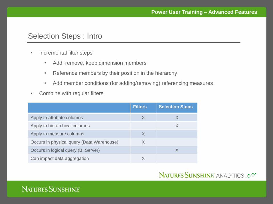
Selection Steps : Intro
• Incremental filter steps
• Add, remove, keep dimension members
• Reference members by their position in the hierarchy
• Add member conditions (for adding/removing) referencing measures
• Combine with regular filters
Filters Selection Steps
Apply to attribute columns X X
Apply to hierarchical columns X
Apply to measure columns X
Occurs in physical query (Data Warehouse) X
Occurs in logical query (BI Server) X
Can impact data aggregation X

Power User Training – Advanced Features
Selection Steps : Where is it?
• Selection Steps are accessed at the
bottom of the Results tab

Power User Training – Advanced Features
Selection Steps : Example
• Example: List top 10 products based on order amount and list sum of
remaining products grouped together

Power User Training – Advanced Features
Selection Steps : Example : Part 1
• First we might try a report with: Order Amount,
Product Name, Rank by Order Amount
• Display Product Name if rank < 11, and sum
all other products and label as ‘Other’

Power User Training – Advanced Features
Selection Steps : Example : Part 1 : Results
• Result is not right, what happened?
WITH
SAWITH0 AS (select sum(case when T392311.W_XACT_TYPE_CODE = 'Regular' then T377244.LOCAL_NET_AMT else 0 end ) as c1
from
W_SALES_ORDER_LINE_A T377244 /* Fact_Agg_W_SALES_ORDER_LINE_A */ ,
W_STATUS_D T389005 /* Dim_W_STATUS_D_Order_Status */ ,
W_XACT_TYPE_D T392311 /* Dim_W_XACT_TYPE_D_Sales_Ordlns */
where ( T377244.XACT_TYPE_WID = T392311.ROW_WID and T377244.ORDER_STATUS_WID = T389005.ROW_WID and T389005.DELETE_FLG =
'N' ) ),
SAWITH1 AS (select distinct T179453.PRODUCT_NAME as c1
from
(SELECT
DATASOURCE_NUM_ID,
INTEGRATION_ID,
PRODUCT_DESCR,
PRODUCT_NAME,
LANGUAGE_CODE
FROM
W_PRODUCT_D_TL
WHERE
LANGUAGE_CODE = 'US'
) T179453)
select D1.c1 as c1, D1.c2 as c2, D1.c3 as c3
from ( select distinct 0 as c1,
D1.c1 as c2,
case when Case when D1.c1 is not null then Rank() OVER ( ORDER BY D1.c1 DESC NULLS LAST ) end < 11 then D2.c1 else
'Others' end as c3
from
SAWITH0 D1,
SAWITH1 D2 ) D1 where rownum <= 300001
Power User Training – Advanced Features
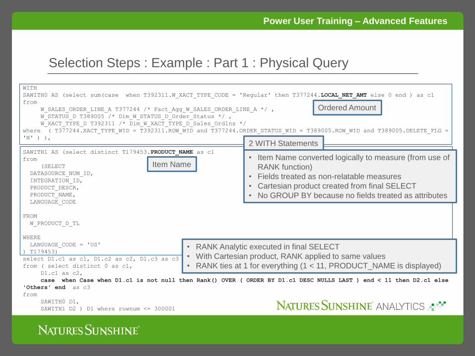
Selection Steps : Example : Part 1 : Physical Query
Item Name
Ordered Amount
2 WITH Statements
• Item Name converted logically to measure (from use of
RANK function)
• Fields treated as non-relatable measures
• Cartesian product created from final SELECT
• No GROUP BY because no fields treated as attributes
• RANK Analytic executed in final SELECT
• With Cartesian product, RANK applied to same values
• RANK ties at 1 for everything (1 < 11, PRODUCT_NAME is displayed)

Power User Training – Advanced Features
Selection Steps : Example : Part 1 : Query Result Sets
select sum(case when T392311.W_XACT_TYPE_CODE = 'Regular' then T377244.LOCAL_NET_AMT else 0 end ) as c1
from
W_SALES_ORDER_LINE_A T377244 /* Fact_Agg_W_SALES_ORDER_LINE_A */ ,
W_STATUS_D T389005 /* Dim_W_STATUS_D_Order_Status */ ,
W_XACT_TYPE_D T392311 /* Dim_W_XACT_TYPE_D_Sales_Ordlns */
where ( T377244.XACT_TYPE_WID = T392311.ROW_WID and T377244.ORDER_STATUS_WID = T389005.ROW_WID and
T389005.DELETE_FLG = 'N' )
SAWITH1 AS (select distinct T179453.PRODUCT_NAME as c1
from
(SELECT
DATASOURCE_NUM_ID,
INTEGRATION_ID,
PRODUCT_DESCR,
PRODUCT_NAME,
LANGUAGE_CODE
FROM
W_PRODUCT_D_TL
WHERE
LANGUAGE_CODE = 'US')
1st WITH
2nd WITH

Power User Training – Advanced Features
Selection Steps : Example : Part 1 : RANK
Final SELECT (with additional RANK field added to see Rank of 1)
select D1.c1 as c1, D1.c2 as c2, D1.c3 as c3, c4
from ( select distinct 0 as c1,
D1.c1 as c2,
case when Case when D1.c1 is not null then Rank() OVER ( ORDER BY D1.c1 DESC NULLS LAST )
end < 11 then D2.c1 else 'Others' end as c3,
Rank() OVER ( ORDER BY D1.c1 DESC NULLS LAST ) as c4
from
SAWITH0 D1,
SAWITH1 D2 ) D1 where rownum <= 300001
• There is nothing to join on, so a Cartesian
product is created
• All products ranked equally
• RANK applied against a Cartesian product
• RANK and other Oracle Analytic functions apply after
the result set returns as they are intra-row functions
Power User Training – Advanced Features
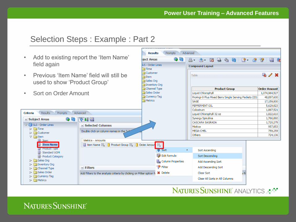
Selection Steps : Example : Part 2
• Add to existing report the ‘Item Name’
field again
• Previous ‘Item Name’ field will still be
used to show ‘Product Group’
• Sort on Order Amount

Power User Training – Advanced Features
Selection Steps : Example : Part 2 : Physical Query
• The query now relates results from the first result set with the second
• A GROUP BY is also applied
OBISUBWITH0 AS (select D1.c1 as c1
from
(select D1.c2 as c1,
Case when D1.c1 is not null then Rank() OVER ( ORDER BY D1.c1 DESC NULLS LAST ) end as c2
from
(select sum(case when T392311.W_XACT_TYPE_CODE = 'Regular' then T377244.LOCAL_NET_AMT else 0 end ) as c1,
T179453.PRODUCT_NAME as c2
from
(SELECT DATASOURCE_NUM_ID, INTEGRATION_ID, PRODUCT_DESCR, PRODUCT_NAME, LANGUAGE_CODE
FROM W_PRODUCT_D_TL
WHERE LANGUAGE_CODE = 'US'
) T179453,
W_PRODUCT_D T186904 /* Dim_W_PRODUCT_D */ ,
W_SALES_ORDER_LINE_A T377244 /* Fact_Agg_W_SALES_ORDER_LINE_A */ ,
W_STATUS_D T389005 /* Dim_W_STATUS_D_Order_Status */ ,
W_XACT_TYPE_D T392311 /* Dim_W_XACT_TYPE_D_Sales_Ordlns */
where ( T179453.DATASOURCE_NUM_ID = T186904.DATASOURCE_NUM_ID and T179453.INTEGRATION_ID =
T186904.INTEGRATION_ID and T186904.ROW_WID = T377244.PRODUCT_WID and T377244.XACT_TYPE_WID = T392311.ROW_WID and
T377244.ORDER_STATUS_WID = T389005.ROW_WID and T389005.DELETE_FLG = 'N' )
group by T179453.PRODUCT_NAME ) D1
) D1
where ( D1.c2 <= 11 ) ),
1st WITH
WITH Name
GROUP BY

Power User Training – Advanced Features
Selection Steps : Example : Part 2 : Physical Query
• 2nd WITH relates to product from 1st WITH
SAWITH0 AS (
select
sum(case when T392311.W_XACT_TYPE_CODE='Regular' then T377244.LOCAL_NET_AMT else 0 end) as c1,
T179453.PRODUCT_NAME as c2
from
(SELECT DATASOURCE_NUM_ID, INTEGRATION_ID, PRODUCT_DESCR, PRODUCT_NAME, LANGUAGE_CODE
FROM W_PRODUCT_D_TL
WHERE LANGUAGE_CODE = 'US'
) T179453,
W_PRODUCT_D T186904 /* Dim_W_PRODUCT_D */ ,
W_SALES_ORDER_LINE_A T377244 /* Fact_Agg_W_SALES_ORDER_LINE_A */ ,
W_STATUS_D T389005 /* Dim_W_STATUS_D_Order_Status */ ,
W_XACT_TYPE_D T392311 /* Dim_W_XACT_TYPE_D_Sales_Ordlns */
where (
T179453.DATASOURCE_NUM_ID = T186904.DATASOURCE_NUM_ID
and T179453.INTEGRATION_ID = T186904.INTEGRATION_ID
and T186904.ROW_WID = T377244.PRODUCT_WID
and T377244.XACT_TYPE_WID = T392311.ROW_WID
and T377244.ORDER_STATUS_WID = T389005.ROW_WID
and T389005.DELETE_FLG = 'N'
and T179453.PRODUCT_NAME in
(select distinct D1.c1 as c1
from OBISUBWITH0 D1 ))
group by T179453.PRODUCT_NAME order by c2 )
2nd WITH
Relate to Product from 1st WITHGROUP BY

Power User Training – Advanced Features
Selection Steps : Example : Part 2 : Incorrect Results
• ‘Others’ Product Group seems low
• That is because it is wrong, CASE
statement is only changing the value
of the name for the 11th product

Power User Training – Advanced Features
Selection Steps : Example : Part 2 : Order Amount Formula
• Change the formula of Order Amount
1) If ranked 1 – 10, then
show the Ordered Amount SUM
grouped by the Product/Item
2) Else, take the total Ordered
Amount for all products and
subtract from the total the
values for products ranked 1 –
10 so we are left with the
remaining SUM of products 11+

Power User Training – Advanced Features
Selection Steps : Example : Part 2 : New Results
• Each product ranked higher than 10th shows the SUM of all
products ranked higher than 10th per the CASE statement
• Each product ranked higher than 10th shows the value of
‘Others’ as it’s product group per the CASE statement for
Product Group

Power User Training – Advanced Features
Selection Steps : Example : Part 2 : RANK
• Add a Rank field and sort ascending on that field to see the
top 10 products based on rank
Power User Training – Advanced Features
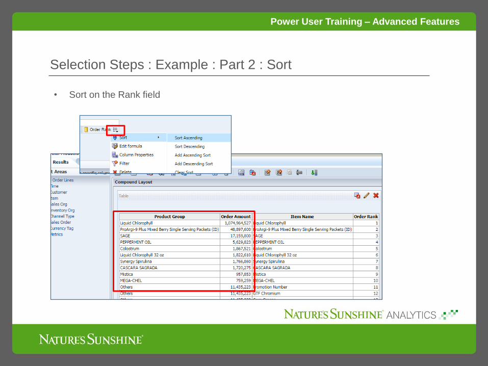
Selection Steps : Example : Part 2 : Sort
• Sort on the Rank field

Power User Training – Advanced Features
Selection Steps : Example : Add Selection Step
• Use Selection Steps to keep only the top 11 rows (top 10
products plus ‘Others’ group)

Power User Training – Advanced Features
Selection Steps : Example : Selection Step Results
• Results after Selection
Step of Order Amount
for Top 10 products
compared to total Order
Amount of all other
products

Power User Training – Advanced Features
Selection Steps : Example : Hide Columns
• Hide columns that are not essential for the end user to see
2). Left click edit icon next
to object, then select Hidden
1). Click edit icon on view

Power User Training – Advanced Features
Selection Steps : Example : Alternative Hide Columns
• Hide columns quickly by right clicking the column header area
in the Results tab
Power User Training – Advanced Features
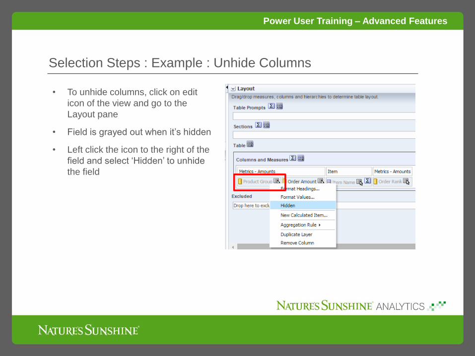
Selection Steps : Example : Unhide Columns
• To unhide columns, click on edit
icon of the view and go to the
Layout pane
• Field is grayed out when it’s hidden
• Left click the icon to the right of the
field and select ‘Hidden’ to unhide
the field

Power User Training – Advanced Features
Selection Steps : Example : Graph
• Add a new graph view
• Notice issue when comparing
large with small amounts on the
same graph
• Issue also with ‘Others’ group
showing an Item Name with it
Large scale makes it difficult to
compare small with large valuesc

Power User Training – Advanced Features
Selection Steps : Example : Graph : Visualization
• Improve visualization of product sales comparison by using Log Base 10 function
or Log (natural log) function
• Add Order Amount measure again
• Copy logic (edit formula) from existing Order Amount measure on report, then
apply Log10 or Log (natural log) – Shown on Next Slide

Power User Training – Advanced Features
Selection Steps : Example : Graph : Visualization
• Apply Log base 10 or Log function to measure logic
• Optionally add sort on LOG Base 10 measure

Power User Training – Advanced Features
Selection Steps : Example : Graph : Hide Columns Globally
• Graph views do not have a hide column feature that’s specific for that view
• Hide Item Name in Criteria tab to have hidden from Graph and all other views
• With Item Name hidden, only Product Group value will show on graph
• Hidden columns are still used in database query

Power User Training – Advanced Features
Selection Steps : Example : Graph : Update Layout
• Move LOG Base 10 Measure
into Measures area of Layout
pane for graph
• Keep Item Name in Group By
area so it’s applied to the
database query; the field
values just won’t show in the
view
• ‘Excluded’ fields will not be
part of the database query

Power User Training – Advanced Features
Selection Steps : Example : Graph : Using LOG Summary
• Good data visualization for data with a very large range is accomplished
with the LOG (natural log) or LOG10 (log base 10) functions
• This example uses LOG10; LOG will scale out to 22 (in this example) with
bars being slightly more spread apart
• Showing the graph side by side with tabular data helps the user visualize
how each product in the top 10 compares to all products while being able
to also review exact values

Real Time
Real Time w/Fragmenting

Real Time
Base Data Model
• Customer Value Score Fact
• Sales Orders Fact
• Web Page Visits Fact

WITHSAWITH0 AS (select sum(T29.ORDER_TOTAL_AMOUNT) as c1,
T13.STATE_REGION as c2from
CUSTOMER_DIM T13,SALES_ORDER_HEADER_FACT T29
where ( T13.CUSTOMER_KEY = T29.CUSTOMER_KEY )group by T13.STATE_REGION)select D1.c1 as c1, D1.c2 as c2, D1.c3 as c3 from ( select distinct 0 as c1,
D1.c2 as c2,D1.c1 as c3
fromSAWITH0 D1
order by c2 ) D1 where rownum <= 65001
Real Time
Example Analysis: No Fragmentation
One Physical QueryResults

Real Time
Combine Real Time Data
• Web Activity
• Sales Orders
• Physical layer contains ODS connection for replicated data from multiple
transactional sources

Real Time
Fragmentation / Federation
• Splicing together data from multiple data sources and reported as if from the same
data source
• Configured in the Logical Table Source
• ‘Fragmentation Content’ tells BI Server when to get data from a specific source
• ‘WHERE clause’ filter is passed down to physical query
Fragmentation
Rules
Real Time
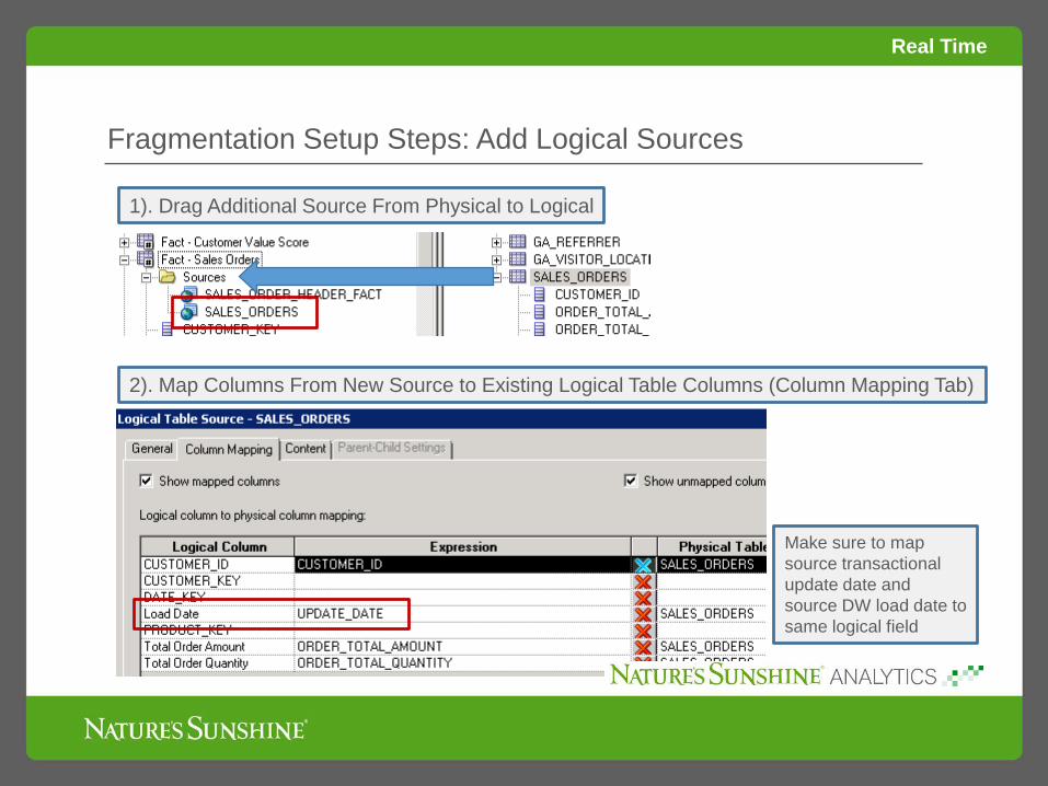
Fragmentation Setup Steps: Add Logical Sources
1). Drag Additional Source From Physical to Logical
2). Map Columns From New Source to Existing Logical Table Columns (Column Mapping Tab)
Make sure to map
source transactional
update date and
source DW load date to
same logical field

Real Time
Fragmentation Setup Steps: Fragment DW
3). Add Fragmentation Content Expression For DW Table (Content Tab)
Combine this source
with other sources to
include data from both
sources in query

Real Time
Fragmentation Setup Steps: Fragment Other Sources
4). Add Fragmentation Content Expression For Other Source(s)
For transactional
sources, include
WHERE clause for
physical query

Real Time
Fragmentation Setup Steps: Repository Variable
Example uses V_ETL_LOAD_DATE as Repository Variable
• Created repository variable with initialization block obtaining MAX(LOAD_DATE) from
ETL_LOAD_DATES table
• Load DW data for dates at or before load date; Load transactional data for the rest

Real Time
Example Analysis: Fragmentation
• Fragmentation also applied to dimensions
• Load Date variable set to 3/27/16
Real Time
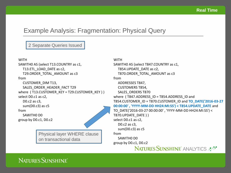
Example Analysis: Fragmentation: Physical Query
WITHSAWITH0 AS (select T13.COUNTRY as c1,
T13.ETL_LOAD_DATE as c2,T29.ORDER_TOTAL_AMOUNT as c3
fromCUSTOMER_DIM T13,SALES_ORDER_HEADER_FACT T29
where ( T13.CUSTOMER_KEY = T29.CUSTOMER_KEY ) )select D0.c1 as c2,
D0.c2 as c3,sum(D0.c3) as c5
fromSAWITH0 D0
group by D0.c1, D0.c2
WITHSAWITH0 AS (select T847.COUNTRY as c1,
T854.UPDATE_DATE as c2,T870.ORDER_TOTAL_AMOUNT as c3
fromADDRESSES T847,CUSTOMERS T854,SALES_ORDERS T870
where ( T847.ADDRESS_ID = T854.ADDRESS_ID and T854.CUSTOMER_ID = T870.CUSTOMER_ID and TO_DATE('2016-03-27 00:00:00' , 'YYYY-MM-DD HH24:MI:SS') < T854.UPDATE_DATE and TO_DATE('2016-03-27 00:00:00' , 'YYYY-MM-DD HH24:MI:SS') < T870.UPDATE_DATE ) )select D0.c1 as c2,
D0.c2 as c3,sum(D0.c3) as c5
fromSAWITH0 D0
group by D0.c1, D0.c2
2 Separate Queries Issued
Physical layer WHERE clause
on transactional data

Real Time
Example Analysis: Fragmentation: Logical Query
DetailFilter: ADDRESSES.ADDRESS_ID = CUSTOMERS.ADDRESS_ID and CUSTOMERS.CUSTOMER_ID = SALES_ORDERS.CUSTOMER_ID and TIMESTAMP '2016-03-27 00:00:00.000' < CUSTOMERS.UPDATE_DATE and TIMESTAMP '2016-03-27 00:00:00.000' < SALES_ORDERS.UPDATE_DATE
Fragmentation filter applied

Automate Deployment
Automating OBIEE Deployment

Automate Deployment
Manual Deployment: Deploy Steps
1). Get RPD File (and change password)
2). Deploy in Enterprise Manager
3). Restart
4). Update User/Pass/JDBC

Automate Deployment
Manual Deployment: Risk
• Time to deploy: 25 minutes (large implementation)
• Risk
• Upload wrong RPD
• Forget to change password to target password
• Enter wrong password when deploying in Enterprise Manager
• Forget to update database user/pass after deploy
• Enter wrong database user/pass after deploy
• Need longer maintenance window because of risk (45 minutes)

Automate Deployment
Automated Deployment: Deploy Steps
1). Execute Script
2). Optionally watch the process

Automate Deployment
Automated Deployment: Risk
• Time to deploy: 3 minutes
• Risk
• Execute script against wrong environment
• Maintenance window: 5 minutes

Automate Deployment
Automated Deployment: Setup
1). Create target connections patch file
• Save RPD as XML
• Can use text editor program or utility
(like sed) to extract ‘ConnectionPool’
lines:
• sed -n '/<ConnectionPool name/,/<\/ConnectionPool>/p' rpd.xml > connection_pools.xml
• Add XML root, repository and declare nodes
• <?xml version="1.0" encoding="UTF-8" ?><Repository xmlns:xsi="http://www.w3.org/2001/XMLSchema-instance"><DECLARE>...<ConnectionPool> lines ...</DECLARE></Repository>

Automate Deployment
Automated Deployment: Setup
2). Download Rittman Deploy w/Restart Script
• http://www.oracle.com/technetwork/issue-archive/2011/11-nov/o61bi-486594.html
• Auto deploy script will call this to deploy updated RPD in target environment
3). Download Auto Deploy Script Associated With This Presentation at UTOUG