object detection as supervised...
TRANSCRIPT

11/9/2015
1
Object detection as supervised classification
Tues Nov 10
Kristen Grauman
UT Austin
Today
• Supervised classification
• Window-based generic object detection
– basic pipeline
– boosting classifiers
– face detection as case study

11/9/2015
2
Recognizing flat, textured
objects (like books, CD
covers, posters)
Reading license plates,
zip codes, checks
Fingerprint recognition
Frontal face detection
What kinds of things work best today?
What kinds of things work best today?

11/9/2015
3
Generic category recognition:
basic framework
• Build/train object model
– (Choose a representation)
– Learn or fit parameters of model / classifier
• Generate candidates in new image
• Score the candidates
Supervised classification
• Given a collection of labeled examples, come up with a
function that will predict the labels of new examples.
• How good is some function we come up with to do the
classification?
• Depends on
– Mistakes made
– Cost associated with the mistakes
“four”
“nine”
?Training examples Novel input

11/9/2015
4
Supervised classification
• Given a collection of labeled examples, come up with a
function that will predict the labels of new examples.
• Consider the two-class (binary) decision problem
– L(4→9): Loss of classifying a 4 as a 9
– L(9→4): Loss of classifying a 9 as a 4
• Risk of a classifier s is expected loss:
• We want to choose a classifier so as to minimize this
total risk
49 using|49Pr94 using|94Pr)( LsLssR
Supervised classification
Feature value x
Optimal classifier will
minimize total risk.
At decision boundary,
either choice of label
yields same expected
loss.
If we choose class “four” at boundary, expected loss is:
If we choose class “nine” at boundary, expected loss is:
4)(9 )|9 is class(
4)(4) | 4 is (class4)(9 )|9 is class(
LP
LPLP
x
xx
9)(4 )|4 is class( LP x

11/9/2015
5
Supervised classification
Feature value x
Optimal classifier will
minimize total risk.
At decision boundary,
either choice of label
yields same expected
loss.
So, best decision boundary is at point x where
To classify a new point, choose class with lowest expected
loss; i.e., choose “four” if
9)(4) |4 is P(class4)(9 )|9 is class( LLP xx
)49()|9()94()|4( LPLP xx
P(4 | x) P(9 | x)

11/9/2015
6
Probability
Basic probability
• X is a random variable
• P(X) is the probability that X achieves a certain value
•
• or
• Conditional probability: P(X | Y)
– probability of X given that we already know Y
continuous X discrete X
called a PDF-probability distribution/density function
Source: Stev e Seitz
Example: learning skin colors
• We can represent a class-conditional density using a
histogram (a “non-parametric” distribution)
Feature x = Hue
P(x|skin)
Feature x = Hue
P(x|not skin)
Percentage of skin pixels in each bin

11/9/2015
7
Example: learning skin colors
• We can represent a class-conditional density using a
histogram (a “non-parametric” distribution)
Feature x = Hue
P(x|skin)
Feature x = Hue
P(x|not skin)Now we get a new image,
and want to label each pixel as skin or non-skin.
What’s the probability we
care about to do skin detection?
Bayes rule
)(
)()|()|(
xP
skinPskinxPxskinP
posterior priorlikelihood
)()|( )|( skinPskinxPxskinP
Where does the prior come from?
Why use a prior?

11/9/2015
8
Example: classifying skin pixels
Now for every pixel in a new image, we can
estimate probability that it is generated by skin.
Classify pixels based on these probabilities
Brighter pixels
higher probability
of being skin
Example: classifying skin pixels
Gary Bradski, 1998

11/9/2015
9
Gary Bradski, 1998
Example: classifying skin pixels
Using skin color-based face detection and pose estimation
as a video-based interface
Generative vs. Discriminative Models
• Generative approach: separately model class-conditional
densities and priors
then evaluate posterior probabilities using Bayes’ theorem
• Discriminative approach: directly model posterior
probabilities
• In both cases usually work in a feature space
Slide f rom Christopher M. Bishop, MSR Cambridge

11/9/2015
10
This same procedure applies in more general circumstances
• More than two classes
• More than one dimension
General classification
H. Schneiderman and T.Kanade
Example: face detection
• Here, X is an image region
– dimension = # pixels
– each face can be thoughtof as a point in a high
dimensional space
H. Schneiderman, T. Kanade. "A Statistical Method for 3D Object Detection Applied to Faces and Cars". IEEE Conference
on Computer Vision and Pattern Recognition (CVPR 2000) http://www-2.cs.cmu.edu/afs/cs.cmu.edu/user/hws/www/CVPR00.pdf Source: Stev e Seitz
Today
• Supervised classification
• Window-based generic object detection
– basic pipeline
– boosting classifiers
– face detection as case study

11/9/2015
11
Generic category recognition:
basic framework
• Build/train object model
– Choose a representation
– Learn or fit parameters of model / classifier
• Generate candidates in new image
• Score the candidates
Window-based models
Building an object model
Car/non-car
Classifier
Yes, car.No, not a car.
Given the representation, train a binary classifier

11/9/2015
12
Window-based models
Generating and scoring candidates
Car/non-car
Classifier
Window-based object detection: recap
Car/non-car
Classifier
Feature
extraction
Training examples
Training:1. Obtain training data
2. Define features
3. Define classifier
Given new image:1. Slide window
2. Score by classifier

11/9/2015
13
Discriminative classifier construction
106 examples
Nearest neighbor
Shakhnarovich, Viola, Darrell 2003Berg, Berg, Malik 2005...
Neural networks
LeCun, Bottou, Bengio, Haffner 1998Rowley, Baluja, Kanade 1998…
Support Vector Machines Conditional Random Fields
McCallum, Freitag, Pereira 2000; Kumar, Hebert 2003…
Guyon, Vapnik
Heisele, Serre, Poggio, 2001,…
Slide adapted from Antonio Torralba
Boosting
Viola, Jones 2001, Torralba et al. 2004, Opelt et al. 2006,…
Boosting intuition
Weak
Classifier 1
Slide credit: Paul Viola

11/9/2015
14
Boosting illustration
Weights
Increased
Boosting illustration
Weak
Classifier 2

11/9/2015
15
Boosting illustration
Weights
Increased
Boosting illustration
Weak
Classifier 3

11/9/2015
16
Boosting illustration
Final classifier is
a combination of weak
classifiers
Boosting: training
• Initially, weight each training example equally
• In each boosting round:
– Find the weak learner that achieves the lowest weighted training error
– Raise weights of training examples misclassified by current weak learner
• Compute final classifier as linear combination of all weak
learners (weight of each learner is directly proportional to
its accuracy)
• Exact formulas for re-weighting and combining weak
learners depend on the particular boosting scheme (e.g.,
AdaBoost)Slide credit: Lana Lazebnik

11/9/2015
17
Viola-Jones face detector
Main idea:
– Represent local texture with efficiently computable
“rectangular” features within window of interest
– Select discriminative features to be weak classifiers
– Use boosted combination of them as final classifier
– Form a cascade of such classifiers, rejecting clear
negatives quickly
Viola-Jones face detector

11/9/2015
18
Viola-Jones detector: features
Feature output is difference between
adjacent regions
Efficiently computable
with integral image: any
sum can be computed in
constant time.
“Rectangular” filters
Value at (x,y) is
sum of pixels
above and to the
left of (x,y)
Integral image
Computing the integral image
Lana Lazebnik

11/9/2015
19
Computing the integral image
Cumulative row sum: s(x, y) = s(x–1, y) + i(x, y)
Integral image: ii(x, y) = ii(x, y−1) + s(x, y)
ii(x, y-1)
s(x-1, y)
i(x, y)
MATLAB: ii = cumsum(cumsum(double(i)), 2);
Lana Lazebnik
Computing sum within a rectangle
• Let A,B,C,D be the values of the integral image at the corners of a rectangle
• Then the sum of original image values within the rectangle can be computed as:
sum = A – B – C + D
• Only 3 additions are required for any size of rectangle!
D B
C A
Lana Lazebnik

11/9/2015
20
Viola-Jones detector: features
Feature output is difference between
adjacent regions
Efficiently computable
with integral image: any
sum can be computed in
constant time
Avoid scaling images
scale features directly
for same cost
“Rectangular” filters
Value at (x,y) is
sum of pixels
above and to the
left of (x,y)
Integral image
Considering all
possible filter
parameters: position,
scale, and type:
180,000+ possible
features associated
with each 24 x 24
window
Which subset of these features should we
use to determine if a window has a face?
Use AdaBoost both to select the informative
features and to form the classifier
Viola-Jones detector: features

11/9/2015
21
Viola-Jones detector: AdaBoost
• Want to select the single rectangle feature and threshold that best separates positive (faces) and negative (non-
faces) training examples, in terms of weighted error.
Outputs of a possible rectangle feature on faces and non-faces.
…
Resulting weak classifier:
For next round, reweight the examples according to errors,
choose another filter/threshold
combo.
Perc
eptu
al a
nd S
enso
ry A
ugm
ente
d C
om
puti
ng
Vis
ual O
bje
ct R
eco
gnit
ion T
uto
rial
Vis
ual O
bje
ct R
eco
gnit
ion T
uto
rial
AdaBoost AlgorithmStart with uniform weights on training
examples
Evaluate weighted error for each feature,
pick best.
Re-weight the examples:Incorrectly classified -> more weightCorrectly classified -> less weight
Final classifier is combination of the weak ones, weighted according to error they had.
Freund & Schapire 1995
{x1,…xn}For T rounds

11/9/2015
22
Perc
eptu
al a
nd S
enso
ry A
ugm
ente
d C
om
puti
ng
Vis
ual O
bje
ct R
eco
gnit
ion T
uto
rial
Vis
ual O
bje
ct R
eco
gnit
ion T
uto
rial
First two features selected
Viola-Jones Face Detector: Results
• Even if the filters are fast to compute, each new
image has a lot of possible windows to search.
• How to make the detection more efficient?

11/9/2015
23
Cascading classifiers for detection
• Form a cascade with low false negative rates early on
• Apply less accurate but faster classifiers first to immediately
discard windows that clearly appear to be negative
Training the cascade
• Set target detection and false positive rates for
each stage
• Keep adding features to the current stage until
its target rates have been met • Need to lower AdaBoost threshold to maximize detection (as
opposed to minimizing total classification error)
• Test on a validation set
• If the overall false positive rate is not low
enough, then add another stage
• Use false positives from current stage as the
negative training examples for the next stage

11/9/2015
24
Viola-Jones detector: summary
Train with 5K positives, 350M negativesReal-time detector using 38 layer cascade6061 features in all layers
[Implementation available in OpenCV]
Faces
Non-faces
Train cascade of classifiers with
AdaBoost
Selected features, thresholds, and weights
New image
Viola-Jones detector: summary
• A seminal approach to real-time object detection
• Training is slow, but detection is very fast
• Key ideas
Integral images for fast feature evaluation
Boosting for feature selection
Attentional cascade of classifiers for fast rejection of non-
face windows
P. Viola and M. Jones. Rapid object detection using a boosted cascade of simple features.
CVPR 2001.
P. Viola and M. Jones. Robust real-time face detection. IJCV 57(2), 2004.

11/9/2015
25
Perc
eptu
al a
nd S
enso
ry A
ugm
ente
d C
om
puti
ng
Vis
ual O
bje
ct R
eco
gnit
ion T
uto
rial
Vis
ual O
bje
ct R
eco
gnit
ion T
uto
rial
Viola-Jones Face Detector: ResultsPe
rce
ptu
al a
nd S
enso
ry A
ugm
ente
d C
om
puti
ng
Vis
ual O
bje
ct R
eco
gnit
ion T
uto
rial
Vis
ual O
bje
ct R
eco
gnit
ion T
uto
rial
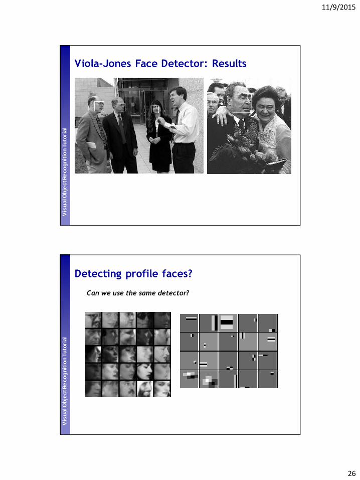
Viola-Jones Face Detector: Results
11/9/2015
26
Perc
eptu
al a
nd S
enso
ry A
ugm
ente
d C
om
puti
ng
Vis
ual O
bje
ct R
eco
gnit
ion T
uto
rial
Vis
ual O
bje
ct R
eco
gnit
ion T
uto
rial
Viola-Jones Face Detector: ResultsPe
rce
ptu
al a
nd S
enso
ry A
ugm
ente
d C
om
puti
ng
Vis
ual O
bje
ct R
eco
gnit
ion T
uto
rial
Vis
ual O
bje
ct R
eco
gnit
ion T
uto
rial
Detecting profile faces?
Can we use the same detector?

11/9/2015
27
Perc
eptu
al a
nd S
enso
ry A
ugm
ente
d C
om
puti
ng
Vis
ual O
bje
ct R
eco
gnit
ion T
uto
rial
Vis
ual O
bje
ct R
eco
gnit
ion T
uto
rial
Paul Viola, ICCV tutorial
Viola-Jones Face Detector: Results
Everingham, M., Sivic , J. and Zisserman, A.
"Hello! My name is... Buffy" - Automatic naming of characters in TV video,
BMVC 2006. http://www.robots.ox.ac.uk/~vgg/research/nface/index.html
Example using Viola-Jones detector
Frontal faces detected and then tracked, character
names inferred with alignment of script and subtitles.

11/9/2015
28
Consumer application: iPhoto
http://www.apple.com/ilife/iphoto/
Slide credit: Lana Lazebnik

11/9/2015
29
Consumer application: iPhoto 2009
Things iPhoto thinks are faces
Slide credit: Lana Lazebnik
Consumer application: iPhoto 2009
Can be trained to recognize pets!
http://www.maclife.com/article/news/iphotos_faces_recognizes_cats
Slide credit: Lana Lazebnik

11/9/2015
30
Privacy Gift Shop – CV Dazzle
http://www.wired.com/2015/06/facebook-can-recognize-even-dont-show-face/
Wired, June 15, 2015
Privacy Visor
http://www.3ders.org/articles/20150812-japan-3d-printed-privacy-visors-will-block-facial-recognition-software.html

11/9/2015
31
Boosting: pros and cons
• Advantages of boosting• Integrates classification with feature selection
• Complexity of training is linear in the number of training
examples
• Flexibility in the choice of weak learners, boosting scheme
• Testing is fast
• Easy to implement
• Disadvantages• Needs many training examples
• Other discriminative models may outperform in practice
(SVMs, CNNs,…)
– especially for many-class problems
Slide credit: Lana Lazebnik
Perc
eptu
al a
nd S
enso
ry A
ugm
ente
d C
om
puti
ng
Vis
ual O
bje
ct R
eco
gnit
ion T
uto
rial
Vis
ual O
bje
ct R
eco
gnit
ion T
uto
rial
Window-based detection: strengths
• Sliding window detection and global appearance
descriptors:
Simple detection protocol to implement
Good feature choices critical
Past successes for certain classes

11/9/2015
32
Perc
eptu
al a
nd S
enso
ry A
ugm
ente
d C
om
puti
ng
Vis
ual O
bje
ct R
eco
gnit
ion T
uto
rial
Vis
ual O
bje
ct R
eco
gnit
ion T
uto
rial
Window-based detection: Limitations
• High computational complexity
For example: 250,000 locations x 30 orientations x 4 scales =
30,000,000 evaluations!
If training binary detectors independently, means cost increases
linearly with number of classes
• With so many windows, false positive rate better be low
Perc
eptu
al a
nd S
enso
ry A
ugm
ente
d C
om
puti
ng
Vis
ual O
bje
ct R
eco
gnit
ion T
uto
rial
Vis
ual O
bje
ct R
eco
gnit
ion T
uto
rial
Limitations (continued)
• Not all objects are “box” shaped

11/9/2015
33
Perc
eptu
al a
nd S
enso
ry A
ugm
ente
d C
om
puti
ng
Vis
ual O
bje
ct R
eco
gnit
ion T
uto
rial
Vis
ual O
bje
ct R
eco
gnit
ion T
uto
rial
Limitations (continued)
• Non-rigid, deformable objects not captured well with
representations assuming a fixed 2d structure; or must
assume fixed viewpoint
• Objects with less-regular textures not captured well
with holistic appearance-based descriptions
Perc
eptu
al a
nd S
enso
ry A
ugm
ente
d C
om
puti
ng
Vis
ual O
bje
ct R
eco
gnit
ion T
uto
rial
Vis
ual O
bje
ct R
eco
gnit
ion T
uto
rial
Limitations (continued)
• If considering windows in isolation, context is lost
Figur e cr edit: Der ek Hoiem
Sliding window Detector’s view
11/9/2015
34
Perc
eptu
al a
nd S
enso
ry A
ugm
ente
d C
om
puti
ng
Vis
ual O
bje
ct R
eco
gnit
ion T
uto
rial
Vis
ual O
bje
ct R
eco
gnit
ion T
uto
rial
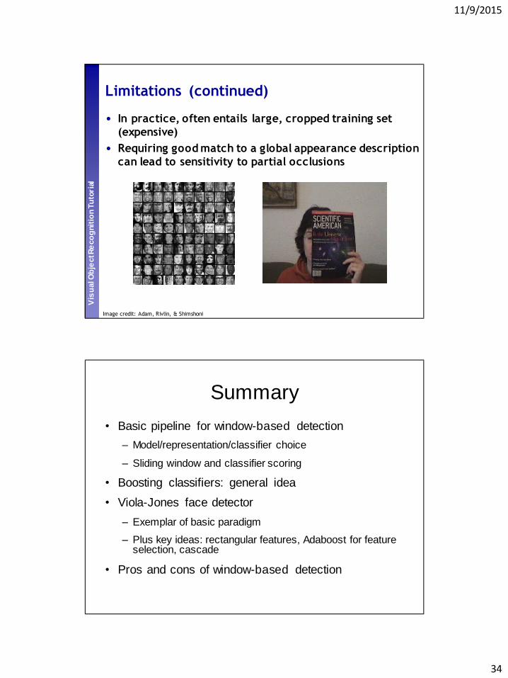
Limitations (continued)
• In practice, often entails large, cropped training set
(expensive)
• Requiring good match to a global appearance description
can lead to sensitivity to partial occlusions
Image credit: Adam, Rivlin, & Shimshoni
Summary
• Basic pipeline for window-based detection
– Model/representation/classifier choice
– Sliding window and classifier scoring
• Boosting classifiers: general idea
• Viola-Jones face detector
– Exemplar of basic paradigm
– Plus key ideas: rectangular features, Adaboost for feature selection, cascade
• Pros and cons of window-based detection