ESM 121

Water Scienceand Management

Exercise 2:

Urban and Agriculture Water Demand

Water Conservation and Water Savings

Samuel Sandoval Solis, PhD

-i-

Table of Contents

Objective..............................................................................................................................1Urban Water Demand..........................................................................................................2

Indoor Water Use.............................................................................................................3Outdoor Water Use........................................................................................................14Future Urban Water Demand.........................................................................................21

-ii-

Objective

The objective of this exercise is to provide examples to estimate:

a) Current water use,

b) Future urban water demands,

c) Agriculture water demands,

d) Irrigation and urban water efficiency, and

e) Water savings.

This exercise will use the population estimation and the Water Use Per Capita (WUPC)

knowledge acquired in the previous exercise (Exercise 1). The concepts in this exercise are very

simple, but they are very illustrative of the complexities involved when estimating future water

demand. This exercise uses the same case of study, the city of Watsonville, now also including

the irrigation area denominated “Pajaro Valley” (Figure 1).

Figure 1 - Watsonville City and Pajaro Valley

1

Urban Water Demand

Urban water use has been divided into two sections, indoor and outdoor water use. Within indoor

water use there is current water use and projected urban water demand. Open the file

Ex_2_Data.xls. In this section we will work on the blue tabs, which are related to urban water

demand. Go to the “Population” tab. Notice that in column D (D17:D25) the population for

Watsonville is already calculated from Exercise 1 (Figure 2)

Figure 2.- Population Tab

Now, let’s move to the “Urban Water Demand” tab. This is the same tab seen in the previous

exercise called “Water Use Per capita” (Figure 3). Just a reminder, in 2010 the Water Use Per

Capita in Watsonville was 120 gpd/person (gallons per day per person), and we will assume that

2012 has the same water use per capita. We will come back later for this number to verify some

of our calculations.

2

Figure 3.- Urban Water Demand Tab

Indoor Water Use

Baseline Scenario

Let’s estimate the indoor water use1 for the Baseline scenario, which represents the current water

use in Watsonville. Indoor water use includes the following uses:

1) Laundry - water used to clean clothes, fabrics and related

2) Dishwashers – water used to wash dishes

3) Faucets – water used in faucets, from washing hands to washing dishes

4) Shower – water used to take a shower

5) Toilet

For laundry water use, Figure 4 shows the water consumption for different types of laundry

machines (vertical and horizontal axis) and models. For the Baseline scenario we are going to

consider a traditional vertical axis machine, 16.1 gpd/person.

1 Cahill, R.J. (2011). Household Water Use and Conservation Models using Monte Carlo techniques for the East

Bay Municipal Utilities District. Master Thesis. Univericity of California, Davis. p. 31-32

3

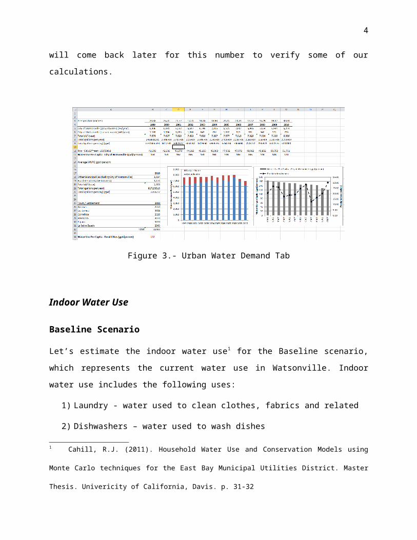
Figure 4

For dishwasher use, Figure 5 shows the water consumption for different types of dishwashers

(high efficiency, average dishwasher and hand washing). For the Baseline scenario we are going

to consider an average dishwasher, 4.7 gpd/person.

Figure 5

So, let’s start calculating the indoor water use in Watsonville. Define the Standard consumption

for Laundry as 16.1 gpd/person and the daily use as 1 per day (Figure 6). The Indoor water use

for the laundry concept is 16.1 gpd/person (Column B * Column D) (Figure 7).

Figure 6

4

Figure 7

Similarly, define that the Standard consumption for a Dishwasher is 4.7 gpd/person and that the

daily use is 1 per day (Figure 8). The Indoor water use for the dishwasher concept is 4.7

gpd/person (cell B10 times cell D10) (Figure 9).

Figure 8

5

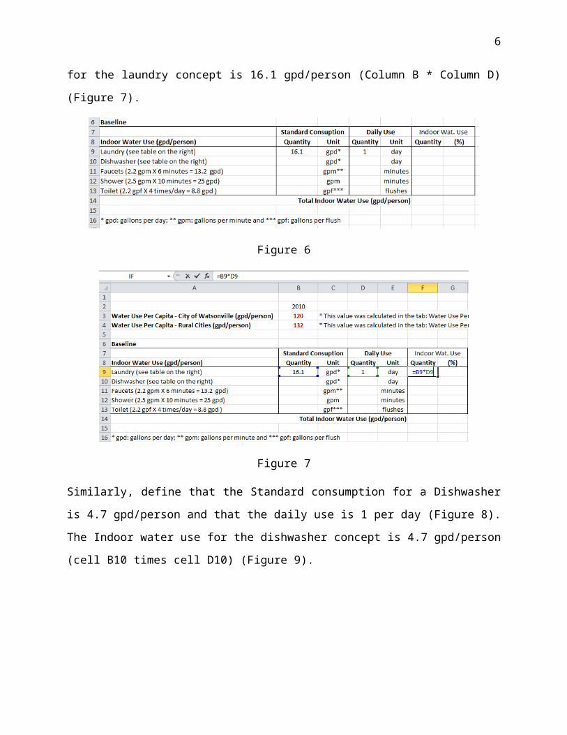
Figure 9

Now, for the faucets (water consumption used to brush your teeth, wash your hands and face,

and rinse the dishes), let’s define the standard flow rate of the faucet as 2.2 gallons per minute

(gpm) and that on average the faucet is open for 6 minutes per day (Figure 10). The indoor water

use for faucets is 13.2 gpd/person (cell B11 times cell D11) (Figure 11).

Figure 10

6

Figure 11

For the shower water consumption, define the standard flow rate of the shower as 2.5 gallons per

minute (gpm) and the average shower length is 10 minutes per day (Figure 12). The indoor water

use for faucets is 25 gpd/person (cell B12 times cell D12) (Figure 13).

Figure 12

7

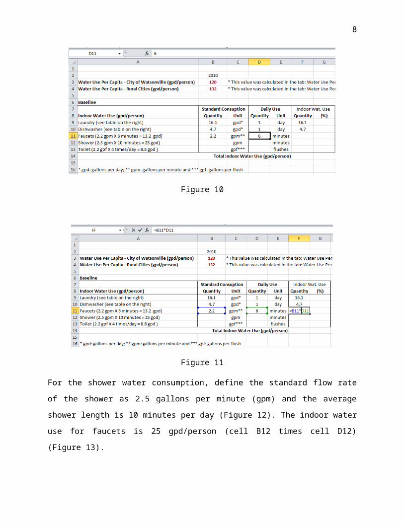
Figure 13

Finally, for the toilet water consumption define the gallons per flush for the standard toilet

considered as 2.2 gallons per flush (gpf) and that the average flushes per day are 4 (Figure 14).

The indoor water use for toilets 8.8 gpd/person (cell B13 times cell D13) (Figure 15).

Figure 14

8

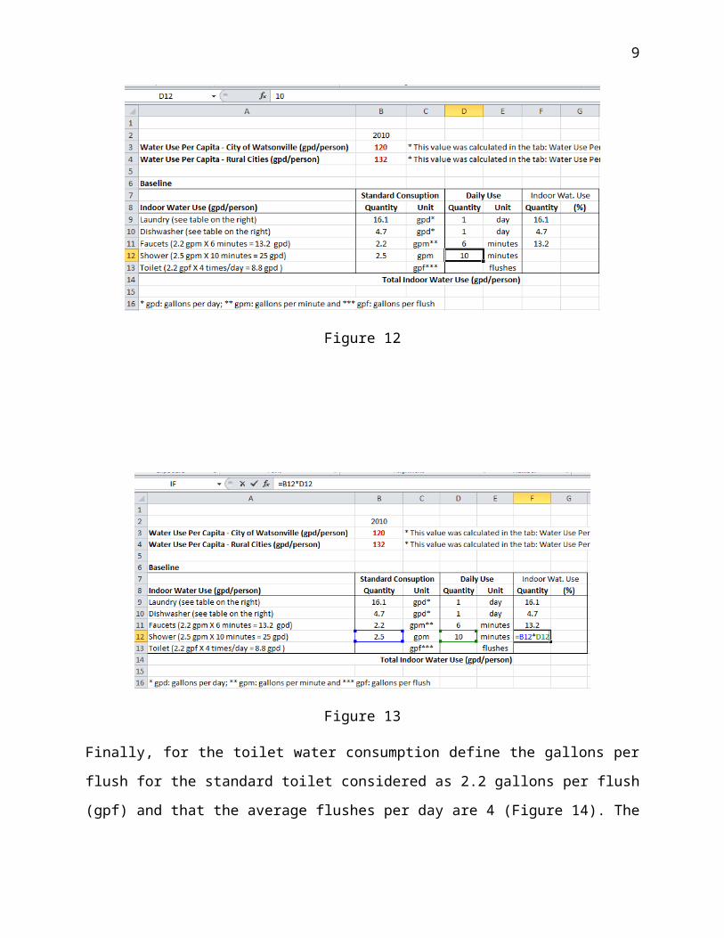
Figure 15

Let’s estimate the indoor daily water user per person by summing all the indoor water use

(Figure 16), which is 67.8 gpd/person

Figure 16

Finally let’s estimate the percentage that each of the concepts represents for the indoor water use

(Figure 17). Notice that shower consumes about one third of the indoor water use (~37%),

laundry a quarter of the use, dishwashers and faucets combined use another quarter (7%

+19%=26% ~ 25%) and toilets use about one eighth of the indoor water use (~13%).

9

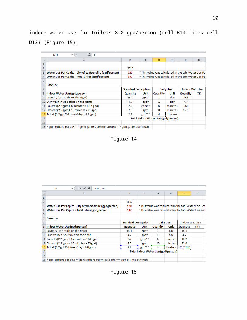
Figure 17

To be turned in: a) a table of the indoor water use, b) Did you have an idea of your indoor water

use before this exercise? Do you think this value is too high? Too low? How does it compare

with other sources? http://www.drinktap.org/consumerdnn/Default.aspx?tabid=85

http://www.h2oconserve.org/wp-content/uploads/2010/11/Indoor-Water-Use-at-Home.pdf

c) Can you compare it to indoor water uses in other countries?

http://www.cbia.org/go/cbia/?LinkServID=E242764F-88F9-4438-9992948EF86E49EA https://www.ec.gc.ca/eau-water/default.asp?lang=En&n=F25C70EC-1

Scenario I –Indoor Conservation

Now, let’s propose that we start conserving water by:

a) Implementing some incentives, such as rebates and component replacements (toilets,

shower nozzles and faucets)

b) Educations campaigns

c) Enforcing new house builders to include water conservation components in their new

home designs

Let’s preserve the daily use quantities and propose the following modifications to the standard

consumptions (Figure 18):

10

Laundry: People are encouraged to switch from vertical axis traditional washers (16.1

gpd/day) to typical horizontal axis washer (6.4 gpd/day),

Dishwashers: People are encouraged to get rid of average dishwashers (4.7 gpd/day) and

start buying high efficiency dishwashers (2.6 gpd/day),

Faucets: Faucet nozzles are switched from 2.2 gpm nozzles to 1.8 gpm nozzles

Showers: Showerheads are swtiched from 2.5 gpm nozzles to 2.0 gpm nozzles.

Toilets: Toilets are switched from 2.2 gpf to 1.8 gpf.

Figure 18

Similarly that in the previous section, let’s estimate the indoor water use of each category by

multiplying the Standard consumption and the daily use (Figure 19). Let’s calculate the total

indoor water use which is 47 gpd/person (Figure 20) and the percentage that each category

represents (Figure 21).

Figure 19

11

Figure 20

Figure 21

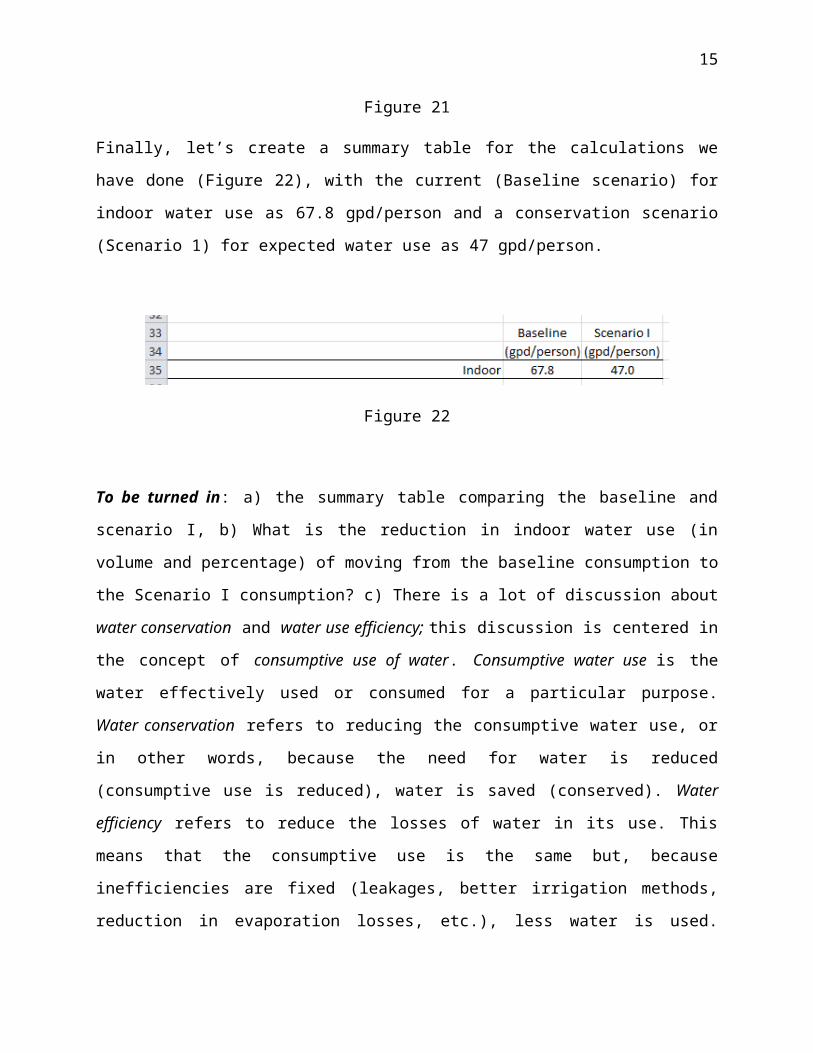
Finally, let’s create a summary table for the calculations we have done (Figure 22), with the

current (Baseline scenario) for indoor water use as 67.8 gpd/person and a conservation scenario

(Scenario 1) for expected water use as 47 gpd/person.

Figure 22

To be turned in: a) the summary table comparing the baseline and scenario I, b) What is the

reduction in indoor water use (in volume and percentage) of moving from the baseline

consumption to the Scenario I consumption? c) There is a lot of discussion about water

conservation and water use efficiency; this discussion is centered in the concept of consumptive

use of water. Consumptive water use is the water effectively used or consumed for a particular

12

purpose. Water conservation refers to reducing the consumptive water use, or in other words,

because the need for water is reduced (consumptive use is reduced), water is saved (conserved).

Water efficiency refers to reduce the losses of water in its use. This means that the consumptive

use is the same but, because inefficiencies are fixed (leakages, better irrigation methods,

reduction in evaporation losses, etc.), less water is used. Question: Can Scenario I be catalogued

as a water conservation or water efficiency policy?

Outdoor Water Use

Evapotranspiration and Water Consumption of Crops and Plants

In this section we will analyze the outdoor water use; using the approach of WUCOLS (2000)2

which depends on different factors:

Geographical location: The mean reference evapotranspiration (ET0) will be used to

account for this.

Mean landscaping area

The type of landscaping: A crop coefficient factor (Kc) will be used to estimate the water

consumption for different types of landscaping

Irrigation efficiency: This factor considers how much of the applied water is beneficial to

the plant

The usual way to estimate the water needs of a plant, crop or, in this case, landscape area

(ETLandscape), is by estimating the Evapotranspiration of that area (ETLandscape, or Evapotranspiration

of the Landscape) (Equation 1). Every crop needs a different amount of water, so here is how

ETLandscape is estimated. First, you need to know the Reference Evapotranspiration (ET0) of the

region. ET0 is the evapotranspiration of a cool-season grass that is used as a reference value. This

value varies depending on the geographic conditions (latitude, longitude, altitude), and climate

conditions (wind speed, relative humidity/vapor pressure, air temperature solar radiation), so this 2 Water Use Classifications of Landscapes Species (WUCOLS) 2000. “A guide to Estimating Irrigation Water

Needs of Landscape Planting in California” University of California Cooperative Extension, Agriculture and Natural

Resources.

13

value accounts for the geographic position of our study. The crop coefficient (Kc) is a scaling

factor, which is used if the crop in question has a water consumption larger than the reference

evapotranspiration (Kc>1) or smaller than the reference crop (Kc<1). ET0 and ETL are expressed

in units of length (usually inches, feet or centimeters), so, if a Landscape has a

evapotranspiration (ETLandscape) of 36 inches, it means that this crop needs a water depth of 36

inches for every square foot of crop during the whole crop season to be successfully produced.

E T Lanscape=E T 0∗Kc [1]

With equation 1, we just have the height of water needed. The volume is obtained by multiplying

the height of water needed by the area covered by the crop (Equation 2), which gives us the

volume of water that the crop needs and not a drop more!

WaterET=ET Landscape∗Area∗Conversion factors [2]

In reality, not all the water that is provided to the plant is used in the evapotranspiration process.

Some of it is lost into the ground or to the atmosphere due to evaporation. This depends on a lot

of things (irrigation method such as drip irrigation, sprinklers, drip irrigation; human behavior

such as leaving the irrigation system turned on).The point is, the applied water depends on the

irrigation efficiency as shown in equation 3:

A W Landscape=Water ET

Irr . Efficiency[3]

Baseline Scenario

Let’s apply the previous equations to our case of study, the outdoor water use in the city of

Watsonville. Let’s start with the equation for the evapotranspiration of the landscape (ETLandscape)

(Eq. 1). There is Reference Evapotranspiration (ET0) data already available for the whole state of

California (http://www.cimis.water.ca.gov/). Figure 23 shows the ET0 values for the climate

station of Watsonville (Station 95). The annual average reference evapotranspiration (ET0) is

38.67 inches, which we will approximate as 39 inches for practical purposes. Then the plant

factor for the landscape (crop coefficients Kc) is obtained from a specialized publication for

14

landscape water irrigation needs3. The grass that we are selecting is a cool season turfgrass

(regular grass) that has a Kc value of 0.8. With these values we can estimate the landscape

evapotranspiration using Equation 1 (ETLanscape=ET0*Kc), which is 31.2 inches/year, as shown in

figure 24.

Figure 23 – ET0 values for the Station of Watsonville (95)

Figure 24 – Evapotranspiration of the Landscape (ETLandscape), Baseline Scenario

To estimate the Landscape’s water requirements we will use Equation 2

(WaterET=ETLandscape*Area*Conversion factors). The average yard area in Watsonville is around

3 Water Use Classifications of Landscapes Species (WUCOLS) 2000. “A guide to Estimating Irrigation Water

Needs of Landscape Planting in California” University of California Cooperative Extension, Agriculture and Natural

Resources.

15

3,000 square feet, and the conversion factor to obtain gallons per year is 0.62. The Landscape’s

water requirement (WaterET) is 58,032 gallons/year (Figure 25).

Figure 25 – Landscape’s Water Requirements (WaterET), Baseline Scenario

Then we can obtain the Applied Water by using equation 3 (AWLandscape=WaterET/Irr.Efficiency),

the irrigation efficiency is estimated to be 0.75 (sprinklers). The applied water is 77,376

gallons/year (Figure 26), which represents 212 gallons/day (figure 27).

Figure 26 – Applied Water (AWLandscape), Baseline Scenario

Figure 27

If we consider that the numbers of persons living on a house is 4 persons per house, the Outdoor

water use per capita is 53.0 gpd/person (Figure 28).

16

Figure 28 - Per Capita Landscape’s Water Requirements, Baseline Scenario

Scenario I –Outdoor Conservation

Now, let’s propose that we start conserving water outdoors by implementing some financial

incentives (paying people to change their lawn) to change the type of landscape from a highly

water consumptive (regular grass) to a less consumptive type of grass (native grass).

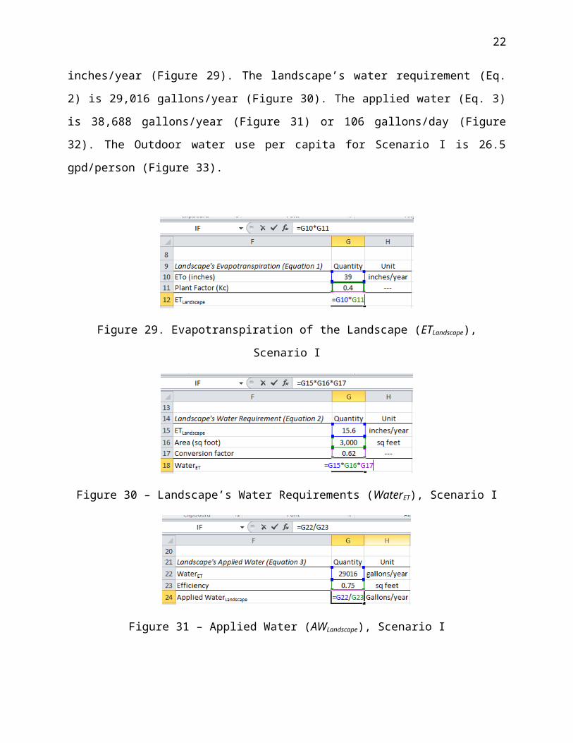
Let’s preserve the rest of the parameters (quantities) and just modify the crop coefficients (Kc)

from 0.8 (regular grass) to 0.4 (native grass). The landscape evapotranspiration (Eq. 1) is 15.6

inches/year (Figure 29). The landscape’s water requirement (Eq. 2) is 29,016 gallons/year

(Figure 30). The applied water (Eq. 3) is 38,688 gallons/year (Figure 31) or 106 gallons/day

(Figure 32). The Outdoor water use per capita for Scenario I is 26.5 gpd/person (Figure 33).

Figure 29. Evapotranspiration of the Landscape (ETLandscape), Scenario I

17

Figure 30 – Landscape’s Water Requirements (WaterET), Scenario I

Figure 31 – Applied Water (AWLandscape), Scenario I

Figure 32

Figure 33 – Per Capita Landscape’s Water Requirements, Scenario I

18

Finally, let’s create a summary table of the Outdoor water use calculations that we’ve done

(Figure 34), with the current (Baseline scenario) indoor water use of 53.0 gpd/person and the

conservation scenario (Scenaio 1) of 26.5 gpd/person.

Figure 34 – Summary Table Outdoors Water Use, Baseline and Scenario I

To be turned in: a) the summary table of the outdoor water uses (such as Fig 34), b) What is the

reduction in outdoor water use (in volume and percentage) of moving from the baseline

consumption to the Scenario I consumption? c) Similar to the indoor analysis, can Scenario I be

catalogued as a water conservation or water efficiency policy? (See the discussion of water

conservation and efficiency on page 13) and d) If we DID NOT change the plant factor “Kc”

(from 0.8 to 0.4) and we proposed to improve the irrigation efficiency by changing the irrigation

method from sprinklers (0.75 efficiency) to drip irrigation (0.95 efficiency), would this new

Scenario II be catalogued as a water conservation or water efficiency policy? Did the

Evapotranspiration of the Landscape (ETLandscape) change or the Landscape’s Water Requirements

(WaterET) change compared to the Baseline Scenario?

Future Urban Water Demand

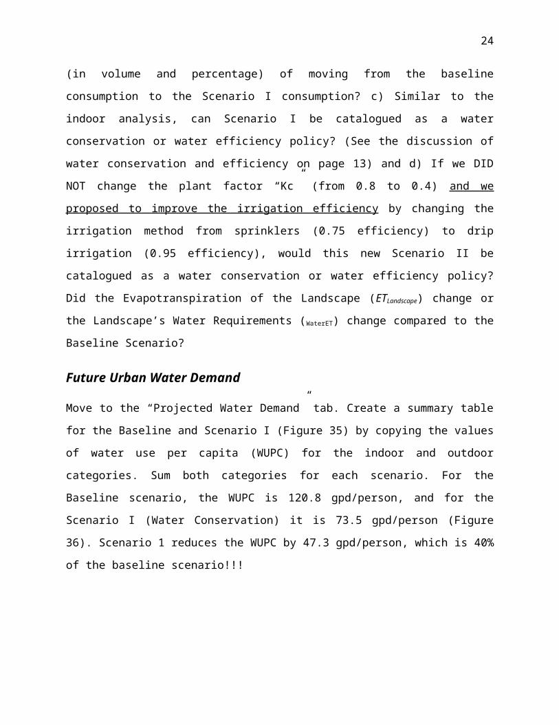
Move to the “Projected Water Demand” tab. Create a summary table for the Baseline and

Scenario I (Figure 35) by copying the values of water use per capita (WUPC) for the indoor and

outdoor categories. Sum both categories for each scenario. For the Baseline scenario, the WUPC

is 120.8 gpd/person, and for the Scenario I (Water Conservation) it is 73.5 gpd/person (Figure

36). Scenario 1 reduces the WUPC by 47.3 gpd/person, which is 40% of the baseline scenario!!!

19

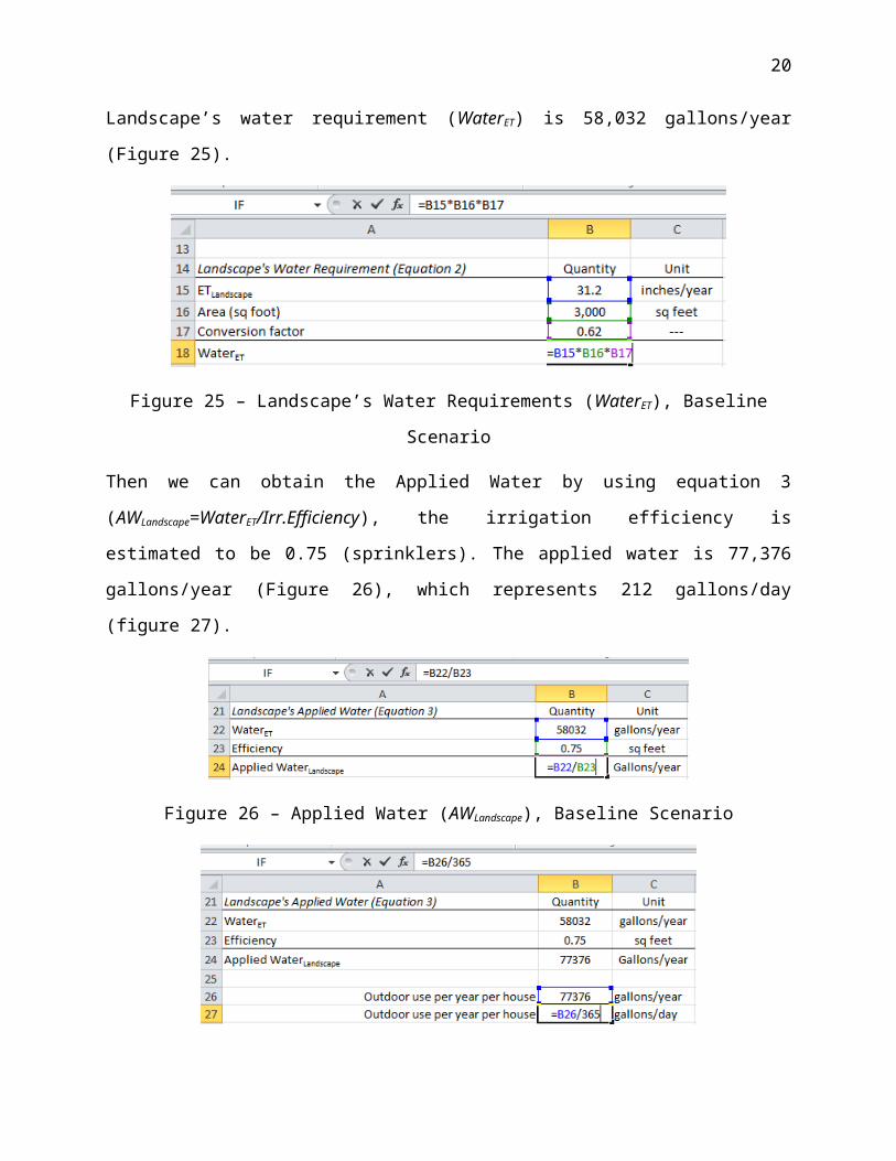
Figure 35

Figure 36

Estimate the share of indoor and outdoor water use for each scenario (Figure 37). Notice that in

the baseline scenario the outdoor water use (44%) is about half of the WUPC, this means that

half of the water is not directly used by the person, it is used to “keep the lawn green.” From the

Baseline to Scenario I, outdoor water use is reduced by half (from 53 gpd/person in the Baseline

Scenario to 26.5 gpd/person in the Scenario I) to about a third (36%) of the WUPC.

Figure 37

To be turned in: a) How much water could be saved indoors (Baseline minus Scenario I)? b)

How much water could be saved outdoors (Baseline minus Scenario I)? c) Where can more

water be saved, indoors or outdoors? d) Before this class, did you realize about the large

consumption of water outdoors compared with indoors? e) Have you noticed that the WUPC for

the Baseline Scenario (120.8 gpd/person) is very similar to the results obtained in Exercise 1

20

(120 gpd/person)!? This is not a coincidence; data was selected carefully to represent the urban

water demand in Watsonville. How do these two calculations support each other? Do you think

having these two calculations makes a stronger argument about their validity and help support

one another?

There are three columns to estimate the future water use for the Baseline Scenario (light orange

color, Figure 38). The first column (Column C) is the water use per capita (WUPC), the second

and third (Column D and E) are the water demand in gallons per year and acre-feet per year,

respectively. The water demand will be calculated until 2030.

Figure 38

21

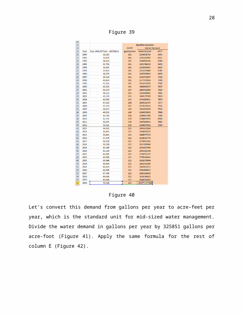
First, let’s estimate the water demand in gallons, which can be obtained by multiplying the

population by the WUPC times 365 days/yr (Figure 39). We had to multiply by 365 days/yr

because the WUPC is in gallons per day per person (gpd/person). Copy the same formula for the

rest of column C (Figure 40).

Figure 39

Figure 40

22

Let’s convert this demand from gallons per year to acre-feet per year, which is the standard unit

for mid-sized water management. Divide the water demand in gallons per year by 325851

gallons per acre-foot (Figure 41). Apply the same formula for the rest of column E (Figure 42).

Figure 41

Figure 42

23

Notice how the chart on the right, it shows the estimated future water demand: If the current

conditions are preserved until 2030 (Baseline scenario), the urban water demand will increase

from ~7,200 AF/year in 2012 to ~9,500 AF/year in 2030, and the city of Watsonville will need

2,300 AF/year more of water which is 32% of the current demand!!! Wwwooww!!!

Now, let’s do a similar procedure to estimate the future water demand for Scenario I (light blue

cell color). In Scenario I, we will consider that every year 5% of the population will move from

the Baseline scenario WUPC (120.8 gpd/person) to a more conservative Scenario I WUPC (73.5

gpd/person). This is represented in columns F and G where it shows the percentage of the

population that is still consuming the WUPC of the Baseline scenario (Column F) and Scenario I

(Column G). In reality, even though as a planner we plan for a smaller water demand, this does

not happen in a blink of an eye. A policy needs time to start working, to develop. This method

of planning also allows us to define goals for the future; e.g. “for 2020, 40% of the population in

Watsonville should be using 73.5 gpd/person or less” or “for 2030, 90% of the population in

Watsonville should be using 73.5 gpd/person or less.” In this way, not only we are proposing

policies, but we are also defining thresholds to be used for monitoring the advancement of the

policy.

To calculate a global WUPC in Watsonville (column H), we will multiply the percentage that is

still using the Baseline WUPC times the Baseline WUPC plus the percentage using Scenario I

WUPC times the Scenario I WUPC (Figure 43), e.g. for 2013 this will be 95%*120.8+5%*73.5

(=F39*$C$10+G39*$E$10). The dollar sign are to fix the WUPC cells (C10 and E10) when

copying the formula. We can calculate this global WUPC for the rest of the years (Figure 44).

Notice that, as Scenario I gains ground, the global WUPC becomes more similar to Scenario I’s

WUPC (73.5 gpd/person).

24

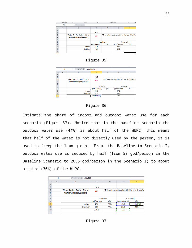
Figure 43

Figure 44

25

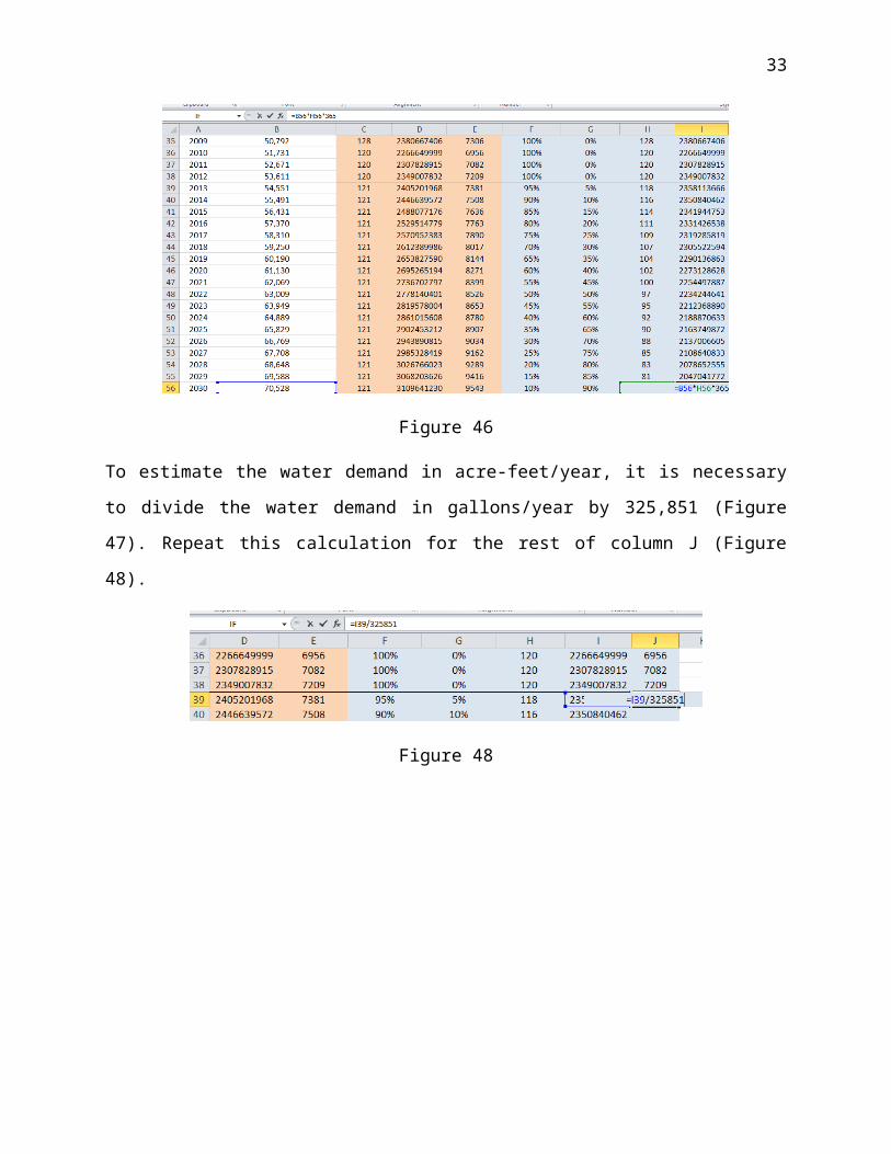
Now let’s do the same procedure as in the previous scenario to calculate the water demand in

gallons per year by multiplying the population (column B) times the global WUPC (Column H)

times 365 days (Figure 45). Copy the same formula for the rest of column I (Figure 46).

Figure 45

Figure 46

To estimate the water demand in acre-feet/year, it is necessary to divide the water demand in

gallons/year by 325,851 (Figure 47). Repeat this calculation for the rest of column J (Figure 48).

Figure 48

26

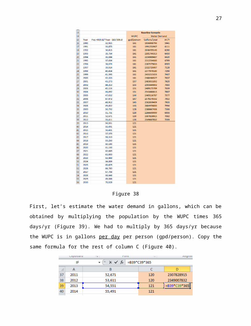
Figure 49

Notice that once again the chart on the right has been modified (Figure 50). While using the

Baseline scenario increases water demand, in Scenario I, when the water conservation is gaining

ground, the water demand starts decreasing. In fact, by conserving water it is possible to go back

to 1990s water demand in 2030!!!

Figure 50

To be turned in: a) Figure 50 (chart) with both water demands, Baseline and Scenario I, b) In

which year will the water demand start to go down? 2014? 2015? 2016?

27

Agriculture Water Demand

Most of the water is used for agriculture, you’ll see. In addition, agricultural water is a hot-hot-

very hot topic in California. People are using water for agriculture but farmers will rarely say

how much water they are using, or let the authorities put in meters to learn how much water

they’ve been using. This does not mean that farmers are wasting water (remember “everyone is

innocent until proven guilty”) In fact, recent trends show that they have been doing better than a

decade ago. What this means is that the job of being a planner is tougher but more interesting.

Please go to the Ag Water Demand Tab (Green Tab) and let’s start with the big picture (Figure

51). According to our calculations for the Baseline scenario, the City of Watsonville is currently

using ~7,209 AF/year (~13%), the rural domestic demand is using 2,508 AF/year (4.5%) and the

agriculture and industrial are using 46,370 AF/Year. Around 82.5% of the water in this region is

being used for Agriculture related purposes!!!!

Figure 51.- Water Uses and Water Demands in Pajaro Valley

Figure 52 and 53 shows the distribution of crops grown in this region; the main crops are

strawberries, vegetable row crops (several types of lettuce, celery, zucchini) and

Raspberries/Blackberries. These three categories add up to 70% of the irrigated area. In fact, a lot

of these commodities in the grocery store come from this area. If we add the 10% of acreage that

is fallowed (nothing is grown here), well, pretty soon we are accounting for 80% of the total

irrigated area in this region, so now we can identify which crops are the big players in this

region.

28

Figure 52.- Crops Acreage

Figure 53 Crop distribution

29

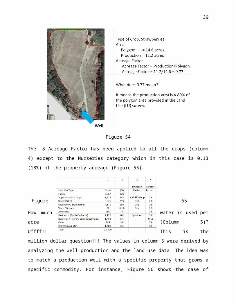
The first step is to calculate the water use for these crops. It is important to clarify that the

acreages that are reported in column 1 are the property acreages and not the production acreages.

In other words, the values in column 1 are the acreage of the properties, but the production area,

which is where the water is applied, is about 80% of the property acreages; take a look at the

calculation shown in Figure 54.

Figure 54

The .8 Acreage Factor has been applied to all the crops (column 4) except to the Nurseries

category which in this case is 0.13 (13%) of the property acreage (Figure 55).

30

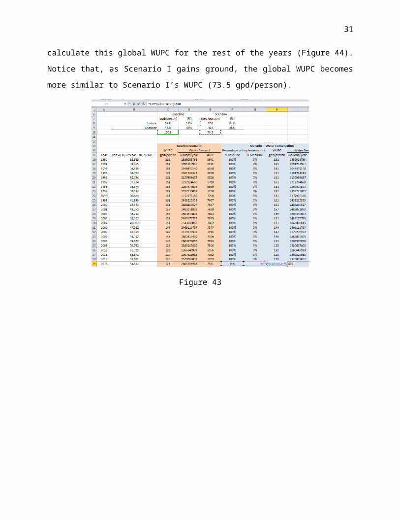
Figure 55

How much water is used per acre (Column 5)? Uffff!! This is the million dollar question!!! The

values in column 5 were derived by analyzing the well production and the land use data. The

idea was to match a production well with a specific property that grows a specific commodity.

For instance, Figure 56 shows the case of using 35AF of water over 11.2 acres of production

area, in which case the water use per acre was 3.1 AF/acre (= 35AF / 11.2 acres)

Figure 56

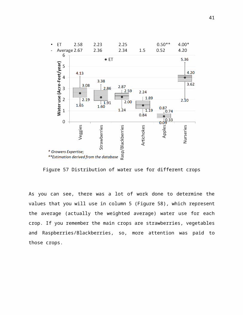
Several properties (polygons) were analyzed and evaluated. Figure 57 shows the distribution of

the water use per acre for each crop- tons of good data!!!. What figure 57 says is that the value

that we are using in column 5 is the average water use per acre for each crop. Notice that in each

crop the water use per acre varied. For instance, for vegetables “veggies” (mostly lettuce), there

were farmers that used 1.65 AF/acre; 50% of the growers used between 2.19 and 3.08 AF/acre,

the average use was 2.67 AF/acre, and some growers used 4.13 AF/acre- as you can see, they

were all over the place!!!!

31

Figure 57 Distribution of water use for different crops

As you can see, there was a lot of work done to determine the values that you will use in column

5 (Figure 58), which represent the average (actually the weighted average) water use for each

crop. If you remember the main crops are strawberries, vegetables and Raspberries/Blackberries,

so, more attention was paid to those crops.

Figure 58

32

The applied water for each crop (column 6) was estimated by multiplying the Acres (column 2)

times the acreage factor (column 4) times the water use per acre (column 5). The formula is

written in the header of column 6 Figure 59.

Figure 59

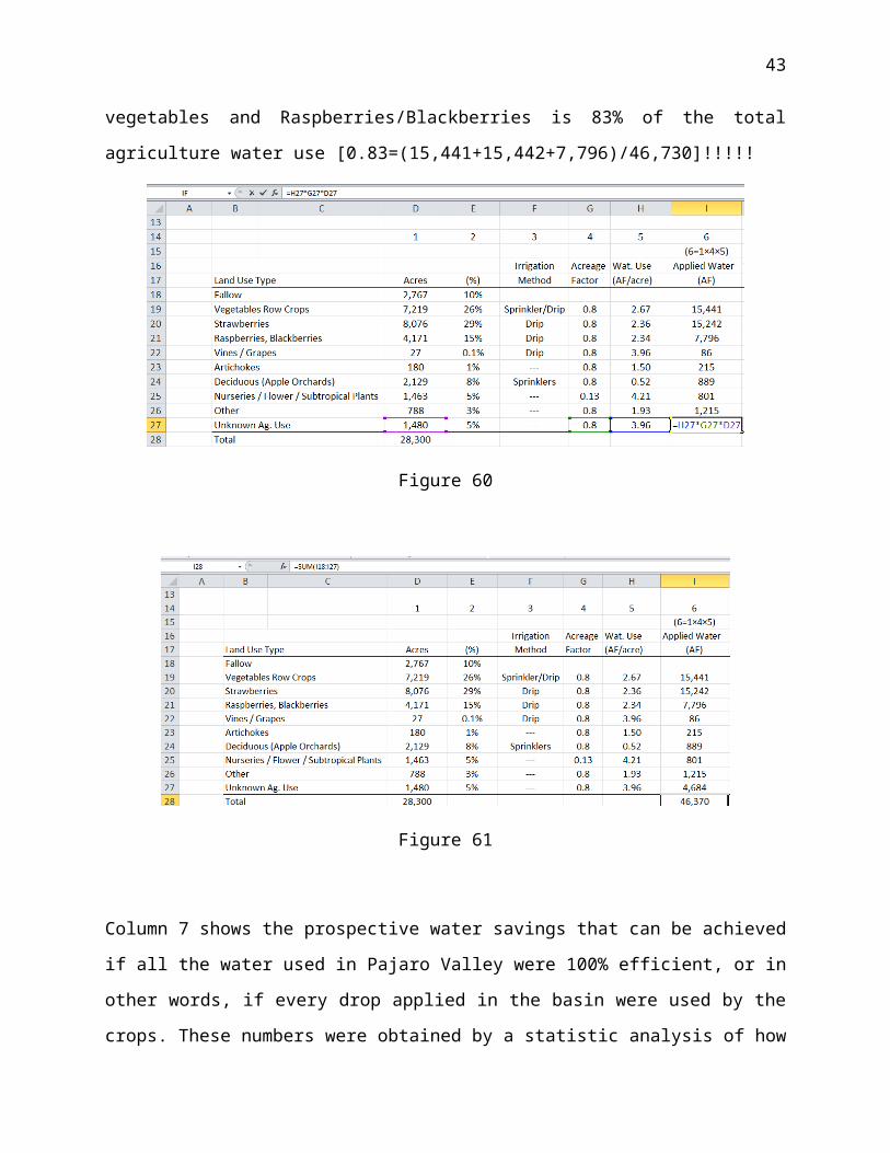
Copying this formula for each crop in Column 6 will help us calculate the agriculture water use

for each crop in Pajaro valley (Figure 60). The total agriculture water use is 46,370 AF/year

(Figure 61) and the water use for strawberries, vegetables and Raspberries/Blackberries is 83%

of the total agriculture water use [0.83=(15,441+15,442+7,796)/46,730]!!!!!

Figure 60

33

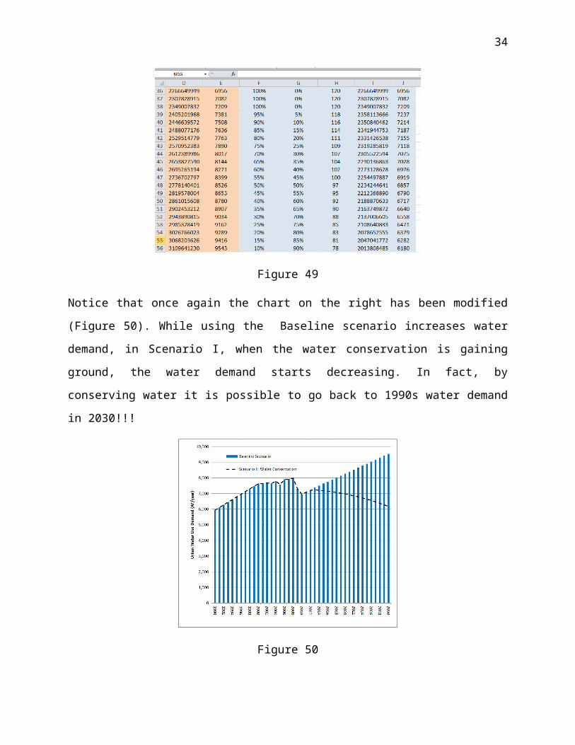
Figure 61

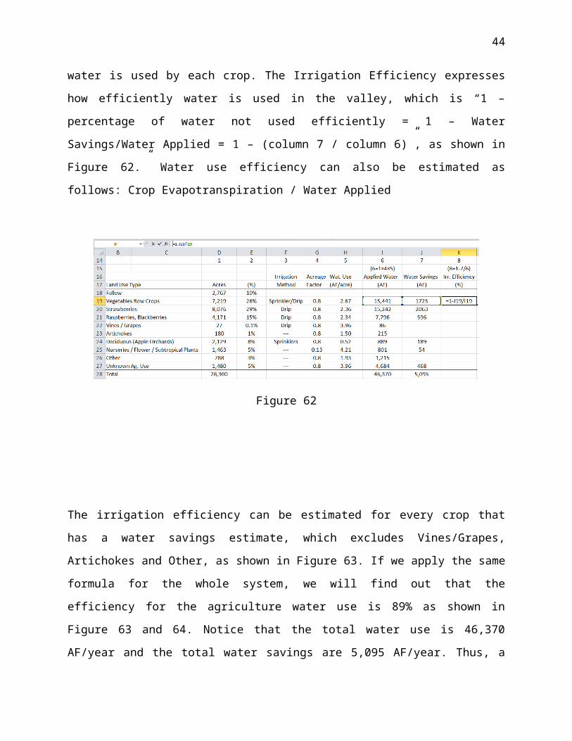
Column 7 shows the prospective water savings that can be achieved if all the water used in

Pajaro Valley were 100% efficient, or in other words, if every drop applied in the basin were

used by the crops. These numbers were obtained by a statistic analysis of how water is used by

each crop. The Irrigation Efficiency expresses how efficiently water is used in the valley, which

is “1 – percentage of water not used efficiently = 1 – Water Savings/Water Applied = 1 –

(column 7 / column 6)”, as shown in Figure 62.” Water use efficiency can also be estimated as

follows: Crop Evapotranspiration / Water Applied

Figure 62

34

The irrigation efficiency can be estimated for every crop that has a water savings estimate, which

excludes Vines/Grapes, Artichokes and Other, as shown in Figure 63. If we apply the same

formula for the whole system, we will find out that the efficiency for the agriculture water use is

89% as shown in Figure 63 and 64. Notice that the total water use is 46,370 AF/year and the total

water savings are 5,095 AF/year. Thus, a rough estimation of the evapotranspiration of the crops

is 41,275 AF/year (46,370 AF/year – 5095 AF-year).

Figure 63

Figure 64

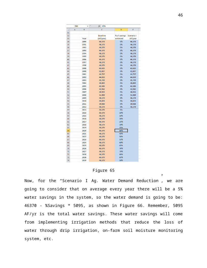
Now, let’s estimate a future water demand for agriculture water use. In the baseline scenario,

let’s consider that on average, the same amount of water will be used, around 46,370 AF/year

(Figure 65), so let’s repeat that value until 2030 in column C.

35

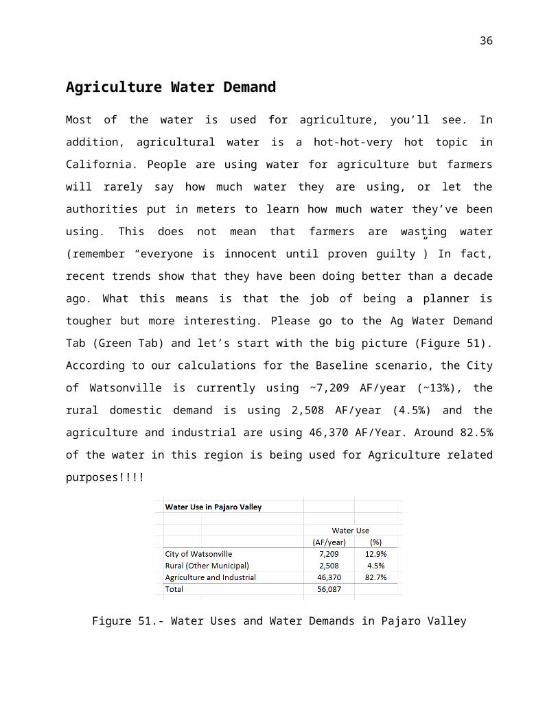
Figure 65

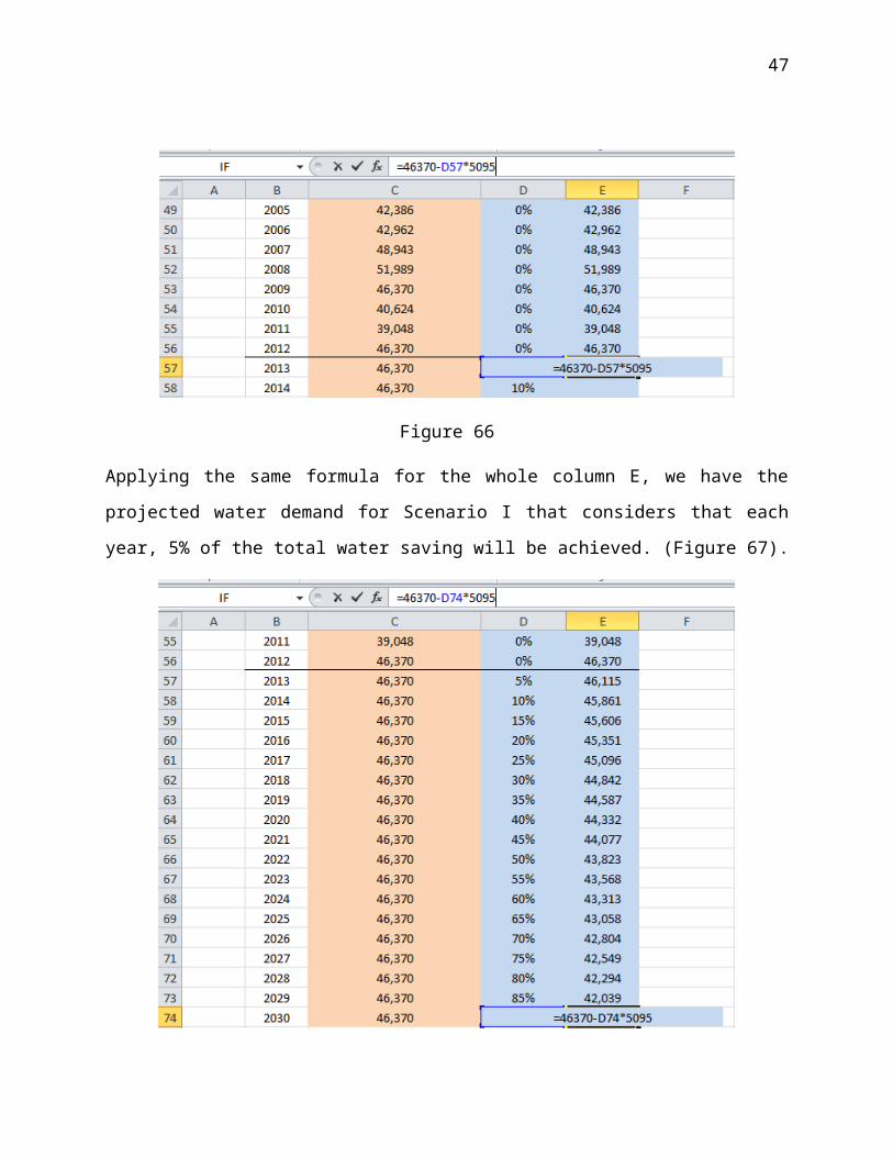
Now, for the “Scenario I Ag. Water Demand Reduction”, we are going to consider that on

average every year there will be a 5% water savings in the system, so the water demand is going

to be: 46370 - %Savings * 5095, as shown in Figure 66. Remember, 5095 AF/yr is the total

water savings. These water savings will come from implementing irrigation methods that reduce

the loss of water through drip irrigation, on-farm soil moisture monitoring system, etc.

36

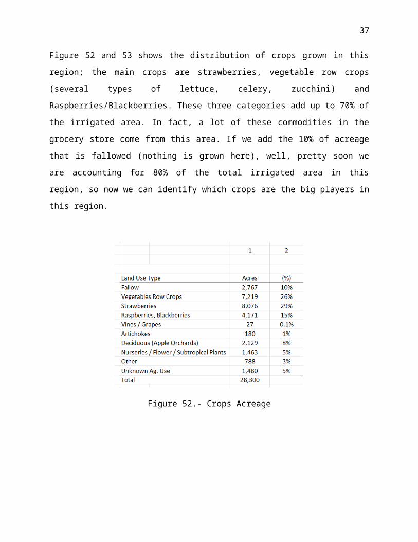
Figure 66

Applying the same formula for the whole column E, we have the projected water demand for

Scenario I that considers that each year, 5% of the total water saving will be achieved. (Figure

67).

Figure 67

37

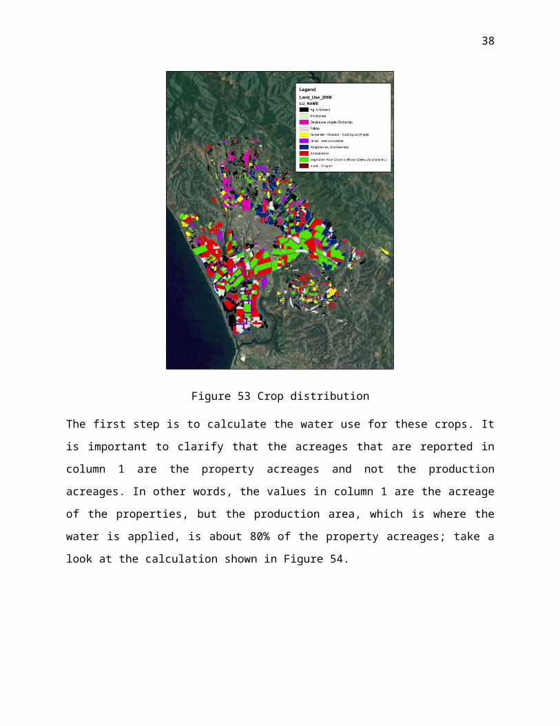
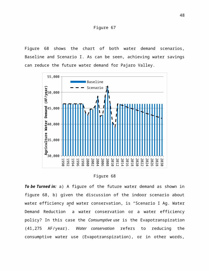
Figure 68 shows the chart of both water demand scenarios, Baseline and Scenario I. As can be

seen, achieving water savings can reduce the future water demand for Pajaro Valley.

199019921994199619982000200220042006200820102012201420162018202020222024202620282030

30,000

35,000

40,000

45,000

50,000

55,000Baseline

Scenario I

Agric

ultu

re W

ater

Dem

and

(AF/

year

)

Figure 68

To be Turned in: a) A figure of the future water demand as shown in figure 68, b) given the

discussion of the indoor scenario about water efficiency and water conservation, is “Scenario I

Ag. Water Demand Reduction” a water conservation or a water efficiency policy? In this case

the Consumptive use is the Evapotranspiration (41,275 AF/year). Water conservation refers to

reducing the consumptive water use (Evapotranspiration), or in other words, because the need for

water is reduced (consumptive use is reduced) water is saved (conserved). Water efficiency refers

to reducing the losses of water in its use, which means that the consumptive use is the same but

because inefficiencies are fixed (leakages, better irrigation methods, reduction in evaporation

losses, and so on) less water is used. Question: Can Scenario I be catalogued as a water

conservation or water efficiency policy?

38

Pajaro Valley Projected Water Demand

Let’s integrate the calculation of urban and agriculture water demands. Let’s move to the tab

“Water Demand Pajaro Valley” (purple tab). There are two set of columns, one for the Baseline

Scenario (orange) and one for Scenario I (light blue) as shown in figure 69.

Figure 69

Actually, we have almost all the data available for every column. Rows 7 and 8 show where the

information is already calculated or how it will be calculated. Let’s start with the baseline

scenario. Column 1 “Municipal” has already been calculated in the “Projected Urban Water

Demand” tab in Column “E”, as it indicates in rows 7 and 8. Let’s get that information by linking

cell “C10” in the current worksheet with cell “E16” in the “Projected Urban Water Demand”

worksheet (as shown in Figure 70). Then let’s copy that same formula for the whole column

(Figure 71)

39

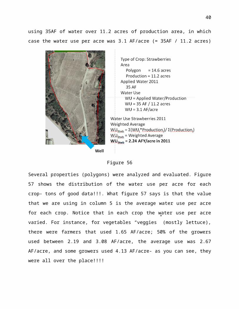
Figure 70

Figure 71

40

Now for Column 2, the baseline calculation for “Rural,” we will consider that the Rural Water

Demand is 35% of the Municipal water demand. That is, multiply Column 1 by a factor of 0.35,

as shown in Figure 72. Figure 73 show the water demand estimation until 2030 for the Rural

sector.

Figure 72

Figure 73

41

For Column 3, the baseline calculation for “Agriculture,” we need to link with the data from the

worksheet “Ag Water Demand” Column “C”. For instance, for year 1990 (Cell “E10”) we need

to recall the data from the worksheet “Ag Water Demand” cell “C34”, as shown in Figure 74.

Figure 75 shows the calculation until 2030.

Figure 74

Figure 75

42

Finally, Column 4 “Total” is the sum of Municipal (column 1), Rural (column 2) and Agriculture

(column 3) as shown in Figure 76. Copy that formula for the whole column. Figure 77 shows the

calculation of the Total baseline water demand until 2030!

Figure 76

Figure 77

43

Now let’s do the same for Scenario I. First, let’s recall the water demand already calculated for

the “Municipal” sector in column 5 of Scenario I from column J of the worksheet “Projected

Urban Water Demand,” as shown in figure 78. Let’s copy that formula for the whole column 5 to

bring the water demand for the Municipal sector of Scenario 1, as shown in Figure 79.

Figure 78

Figure 79

44

Similarly, we will consider that the “Rural” water demand represents 35% of the “Municipal”

water demand as shown in Figure 80. Copy the same formula for all of column 6 of “Rural”

water demand, as shown in figure 81.

Figure 80

Figure 81

45

Data for the “Agriculture” sector, column 7, has to be recalled from the worksheet “Ag Water

Demand” column E, as shown in figure 82. Let’s copy that formula for the whole column 7 to

bring the water demand for the Agriculture sector of Scenario I, as shown in Figure 83.

Figure 82

Figure 83

46

Finally column 8 “Total” is the sum of Municipal (column 5), Rural (column 6) and Agriculture

(column 7) as shown in Figure 84. Copy the formula for the whole column. Figure 85 shows the

calculation of the Total Scenario I water demand until 2030!

Figure 84

Figure 85

47

Let’s take a look at the chart with the water demand under the Baseline scenario and Scenario I

(Figure 86). As can be seen, some of the water efficiency measures proposed in Scenario I can

help save a significant amount of water. The water demand for 2030 for the Baseline and

Scenario I are 59,253 AF/year and 50,128 AF/year, respectively. Even though there was an

increase in population and the value for consumptive water use (evapotranspiration) was

conserved, Scenario I shows that improving the efficiency of the system can help to save water

today and in the future. This type of analysis also helps to define targets to evaluate during the

future implementation of Scenario I.

Figure 86 – Comparison of Water Demands, Baseline Vs. Scenario I

To be turned in: a) A chart similar to Figure 86, b) Is it possible to keep reducing the water

demand in the future? If so, which kind of policies will you apply? Water conservation?

Recycling water? Water harvesting?

48