The Astrophysical Journal, 692:1110–1124, 2009 February 20 doi:10.1088/0004-637X/692/2/1110c© 2009. The American Astronomical Society. All rights reserved. Printed in the U.S.A.

OBSERVATIONAL ANALYSIS OF MAGNETIC RECONNECTION SEQUENCE

Jiong Qiu

Physics Department, Montana State University, Bozeman, MT 59717-3840, USA; qiu@physics.montana.eduReceived 2008 July 17; accepted 2008 October 27; published 2009 February 23

ABSTRACT

We conduct comprehensive analysis of an X2.0 flare to derive quantities indicative of magnetic reconnection in solarcorona by following temporally and spatially resolved flare ribbon evolution in the lower atmosphere. The analysisreveals a macroscopically distinctive two-stage reconnection marked by a clear division in the morphologicalevolution, reconnection rate, and energy release rate. During the first stage, the flare brightening starts at andprimarily spreads along the polarity inversion line (PIL) with the maximum apparent speed comparable to the localAlfven speed. The second stage is dominated by ribbon expansion perpendicular to the PIL at a fraction of the localAlfven speed. We further develop a data analysis approach, namely reconnection sequence analysis, to determinethe connectivity and reconnection flux during the flare between a dozen magnetic sources defined from partitioningthe photospheric magnetogram. It is found that magnetic reconnection proceeds sequentially between magneticcells, and the observationally measured reconnection flux in major cells compare favorably with computationsby a topological model of magnetic reconnection. The three-dimensional evolution of magnetic reconnection isdiscussed with respect to its implication on helicity transfer and energy release through reconnection.

Key words: Sun: activity – Sun: flares – Sun: magnetic fields

Online-only material: color figure

1. INTRODUCTION

Magnetic reconnection governs explosive energy release onthe Sun as manifested in solar flares. In the past decades, obser-vations of flares across the entire atmosphere have given rise tothe standard flare model, which is primarily a two-dimensionalconfiguration. The model captures many macroscopic flare sig-natures (see review by Priest & Forbes 2000) and provides asuccessful qualitative explanation of the evolution and geome-try of the often observed two-ribbon flares (Svestka & Cliver1992). However, magnetic reconnection in the Sun’s corona isthree-dimensional by nature. The observed magnetic field on theSun is highly structured and does not show a two-dimensionalbipolar configuration as in the standard model. Even two-ribbonflares almost always exhibit complex morphologies that can-not be described by a two-dimensional picture. For example,the observed two ribbons in the positive and negative magneticfields are often asymmetric (Fletcher & Hudson 2001), and flarebrightenings are often observed to spread along the ribbon direc-tion (Moore et al. 2001; Fletcher et al. 2004). Furthermore, lackof two-ribbon hard X-ray flares provides strong evidence thatmagnetic energy release is not uniform along the polarity inver-sion line (PIL; Sakao 1994; Krucker et al. 2005). Knowledge ofthe three-dimensional topological structure of the magnetic fieldand its change during the flare is crucial to our understandingof physics of energy storage and release as well as magnetichelicity transfer between topological structures. For the timebeing, such knowledge is only gained from theoretical models(see review by Demoulin 2006).

Recently, Longcope & Beveridge (2007) developed the firstapplicable approach to compute the change of connectivity be-tween topological domains and subsequently the helicity trans-fer between magnetic structures. The model assumes an ini-tial potential field of an active region, which gradually evolvesinto a nonpotential field before the major flare. This is drivenby photospheric plasma motions pushing around magnetic el-ements, whereas the original connectivity is maintained, i.e.,

no reconnection or relaxation is allowed. The build-up of non-potentiality is quantified by the helicity accumulation computedfrom a time sequence of photospheric magnetograms. The pre-flare nonpotential field can only be relaxed through magneticreconnection during the major flare to another potential fieldconstructed from the new boundary, the postflare magnetogram.From the difference between the two potential fields, the modelcan compute the amount and sequence of flux exchange betweentopological domains determined by photospheric magnetic el-ements. Importantly, these physical quantities can be tested byindependent observational measurements, which provides con-straints to the model thus is able to justify or falsify the cal-culation of helicity transfer and energy release by the model.The method was applied to an active region producing an X2.0flare on 2004 November 7 to compute flux exchange betweendomains, helicity transfer, and energy release (Longcope et al.2007).

In this paper, we present an effort toward quantitatively deter-mining evolution of magnetic reconnection from observations.We develop an approach to analyze the connectivity betweenmagnetic cells during magnetic reconnection, which yields therate and sequence of magnetic reconnection to be directly com-pared with the model computation. Reconnection process inthe corona cannot be observed directly but can be tracked viathe temporal and spatial evolution of flare patches in the mag-netic fields in the lower atmosphere, as has been practised bya few groups (Poletto & Kopp 1986; Fletcher & Hudson 2001;Fletcher et al. 2004; Isobe et al. 2002, 2005; Qiu et al. 2002,2004; Saba et al. 2006). In short, following the principle of mag-netic flux conservation from the corona to the lower atmosphereand on typical time and spatial scales of present observations,the coronal magnetic reconnection rate, or reconnection flux perunit time, can be measured by Φ = ∂Φ/∂t = ∂(

∫BldAl)/∂t

(Forbes & Priest 1984). The term on the left denotes the coronalmagnetic reconnection rate, or reconnection flux per unit time.On the right-hand side, Bl is the normal component of magneticfield at the locations of flare patches in the lower atmosphere,

1110

No. 2, 2009 OBSERVATIONAL ANALYSIS OF MAGNETIC RECONNECTION SEQUENCE 1111

(a) 15:49:14 (b) 16:12:41 (c) 16:26:30

TRACE 1600

200 250 300 350E-W (arcsec)

20

40

60

80

100

120

140

S-N

(a

rcse

c)

15:50 16:00 16:10 16:20 16:30Start Time (07-Nov-04 15:47:38)

0

5.0•106

1.0•107

1.5•107

2.0•107

2.5•107

co

un

ts s

-1

flare counts flux

Figure 1. Top: snapshots of the X2.0 flare observed by TRACE 1600 Å on 2004 November 7. Bottom: the light curve of the count rates of the flare at 1600 Å (sameas Figure 7 in Longcope et al. 2007).

which are believed to map the footpoints of field lines reconnect-ing in the corona, and dAl is the elementary newly brightenedflare area at the feet. In this study, we will employ this method tomeasure the temporally and spatially resolved reconnection ratein terms of Φ (in units of Mx s−1) and derive the sequence ofmagnetic reconnection between magnetic sources. In Section 2,we review the X2.0 flare previously modeled by Longcope et al.(2007). In Section 3, we quantitatively examine evolution offlare ribbons with respect to the PIL to gain observational insightinto the three-dimensional evolution of magnetic reconnection.In Section 4, we describe the procedure to derive reconnectionsequence and application to the flare. In Section 5, the analysisresults are briefly compared with the model and discussed re-garding helicity transfer and energy release. Conclusions of thepaper are given in Section 6.

2. TEMPORAL AND SPATIAL EVOLUTION

The standard two-dimensional model assumes a symmetricbipolar configuration and a uniform magnetic reconnection ratealong an infinitely long neutral line in the corona. However, ob-servations reveal that the morphologies of magnetic fields andflares are asymmetric and highly structured. The complex mag-netic field and flare evolution require a full three-dimensionaldescription which deals with both the temporal and spatial evo-lution of magnetic reconnection. To spatially resolve magneticreconnection, in this study, to the first-order approximation, theobserved photospheric magnetic field is partitioned into indi-vidual magnetic cells based on the morphology and evolution ofthe active region (Barnes et al. 2005). Connectivities betweenthese magnetic cells determine the topological structure, whichis often used to describe the magnetic field in the active region(Demoulin et al. 1992, 1994; Longcope 1996).1 Tracking thereconnection rate, inferred from flare evolution, in each of theindividual magnetic cells thus provides the means to determine

1 A thorough investigation on the effects of different ways of partitioning andextrapolation on the field topology is given by Longcope et al. (2009). Theseare not discussed in the present paper, which is focused on the observationalanalysis of reconnection.

the sequence of magnetic reconnection between magnetic do-mains defined by these source elements. In the following text,we refer such analysis as reconnection sequence analysis.

We apply the analysis to a two-ribbon flare occurred at16 UT on 2004 November 7 in NOAA-10696, when the activeregion was at the disk center. The active region was observedby Michelson Doppler Imager (MDI; Scherrer et al. 1995).The flare was observed throughout its evolution by TransitionRegion and Coronal Explorer (TRACE; Handy et al. 1999)in 1600 Å ultraviolet (UV) continuum with the best cadence(2 s) of the instrument and a pixel scale of 0.′′5. Observationsat this wavelength reflect the flare emission in the loweratmosphere, or emission at the feet of flaring loops. Longcopeet al. (2007) comprehensively studied the evolution and topologyof this active region and used a topological model to computeenergy and helicity build-up before the explosion as well ashelicity transfer and energy release during the flare. In thepresent study, flare observations by TRACE and magnetic fieldobservations by MDI are employed to analyze signatures ofmagnetic reconnection and its three-dimensional evolution. InFigure 1, we reproduce the snapshots of the flare and theUV count rates light curve (same as Figure 7 in Longcopeet al. 2007). The flare is composed of two events 40 minutesapart. The first event occurred at 15:40 UT and decayed by16:15 UT. It took place in the core active region. The secondevent set off at 16:25 UT, and resided in the west of the coreregion. In the present study, we limit the analysis to the firstevent. The analysis focuses on quantitative determination ofthe temporal and spatial evolution of magnetic reconnection,which is a crucial step toward understanding the role of magneticreconnection in energy release and helicity transfer.

Figure 2 (top panel) shows the longitudinal magnetogramof the active region obtained by MDI before the flare onset,which is partitioned into a set of positive (denoted by letter “P”)and negative (denoted by the letter “N”) magnetic cells. Weadopt the same partitioning by Longcope et al. (2007), whichis applied to the last magnetogram at the start of the flare. Themagnetic flux in each cell is held constant during the flare withthe assumption that the timescale of magnetic field evolution

1112 QIU Vol. 692

150 200 250 300 350E-W (arcsec)

0

50

100

150

200

S-N

(arc

sec)

P1P2

P3

P4

P5

P6

P7

P8

P9

P13

P15

N1N2

N3 N7N8

N10

N12

magnetic field and flare (contours) on 2004 Nov 7

45 50 55 60 65 70

minutes after 15:00 UT

15 20 25 30 35 40

P1

P2

P3

P4

P5

P6

P7

P8

P9

P13

P15

N1N2

N3N7

N8N10

N12

Figure 2. Top: photospheric magnetogram by MDI superimposed with thecontours of flare areas at the maximum of the flare. “P” and “N” denote thepositive and negative magnetic cells, respectively. Bottom: the temporal andspatial evolution of the flare superimposed on partitioned magnetogram. Timeis indicated by the color code. Specifically, the number below the color barindicates that at the time (minutes after 15:00 UT) indicated by the number, theflare ribbons expand to the areas shaded in the color above this number. Forexample, at 55 minutes after 15:00 UT, the flare ribbons expand to the areasshaded in light blue.

(A color version of this figure is available in the online journal.)

is much longer than the flare duration. Figure 2 (bottom panel)shows the time sequence, as indicated by the color code, offlare brightening observed at 1600 Å superimposed on the co-aligned longitudinal magnetogram. The flare exhibits the wellknown pattern of expanding two bright ribbons, but the magneticfields the ribbons reside in are a lot more complex than a two-dimensional symmetric configuration.

Integrating magnetic flux in flaring regions, we derive timeprofiles of the total reconnection flux Φ(t) in the positiveand negative polarities, as shown in Figure 3. Note that toderive the magnetic flux we use photospheric magnetogramswhich are multiplied by a calibration factor of 1.56 and withprojection effects corrected (Longcope et al. 2007). Differentcalibrations may result in changes in the measured reconnectionflux, but would not affect the time profiles significantly withinthe uncertainties of the measurements (Qiu et al. 2007). In

this study, the time sequence analysis employs 30 s averagedtime profiles of reconnection rates, which significantly reducesfluctuations caused by noise in the magnetograms and byuncertainties in the analysis method (see Qiu et al. 2007). Itis shown that reconnection flux evolves nearly simultaneouslyin both polarities. Theoretically, equal amounts of positive andnegative fluxes should participate in reconnection. We find thatthe median value of the ratio between the total reconnectionfluxes measured in the positive and negative polarities is 1.1,indicating a good balance between the positive and negativefluxes, given that uncertainties in the flux measurements are inthe range of 10%–20% when no magnetic field extrapolation isperformed (Qiu et al. 2007). The reconnection rate Φ(t) in unitsof Mx s−1 is computed as the time derivative of reconnectionflux. On timescales of the order of 1 minute, reconnectionrates Φ(t) derived in the positive and negative polarities arecorrelated: they rise, peak, and decay simultaneously.

Figure 3 shows that magnetic reconnection proceeds in afew episodes. Recognizing major peaks or groups of peaks inthe reconnection rate time profiles, we divide the progress ofreconnection into five episodes as indicated by vertical barsin the figure. These five episodes are also grouped into twomajor stages with an apparent division at 54 minutes after15:00 UT.2 The first stage proceeds for about 10 minutes Thisstage involves about one-third of the total reconnection flux inboth polarities. The second stage sets off with a pronouncedlyincreased reconnection rate, and then reconnection slows downafter 63 minutes. The nominal energy release rate, as indicatedby the time derivative of GOES soft X-ray (1–8 Å) light curve(the so-called “Neupert effect”; Neupert 1968), also exhibits afew peaks, with significant energy release taking place duringthe second stage. An estimate of the thermal energy release rateusing GOES observations and geometric information of the flarewill be given in the last section.

We then derive time profiles of the reconnection rate inmagnetic cells determined from partitioning in Figure 2. A totalof eight positive cells and six negative cells participate in thereconnection at different times during the flare. Reconnectionat two different stages takes place between different pairs ofmagnetic cells. The first stage involves cells right next to thePIL. During this stage, individual flare kernels at a few placesare brightened and then developed into two flare ribbons nearlyalong the PIL. Note that in this event no filament was observedin the active region, and the brightenings in the two ribbonsstarted from the PIL with little separation between the tworibbons at the beginning. During the second stage, most cellsare getting involved, and the two flare ribbons exhibit the well-known pattern of moving apart and nearly perpendicular to thePIL. This main stage of great expansion resembles the two-dimensional arcade-like reconnection (e.g., Moore et al. 2001),and is characterized by evident enhancement in the reconnectionrate and greater amount of reconnection flux as well as energyrelease. Eventually, reconnection ends in a couple of cells adistance away from the PIL.

On macroscopic scales, the first stage is characterized bythe formation of the skeleton of flare ribbons along the PIL,followed by expansion of the ribbons perpendicular to thePIL during the second stage. We, therefore, term these twodistinctive evolution stages as stages of “parallel elongation”and “perpendicular expansion,” respectively. In the following

2 Hereafter, we will record time in terms of minutes after 15:00 UT in bothtext and figures.

No. 2, 2009 OBSERVATIONAL ANALYSIS OF MAGNETIC RECONNECTION SEQUENCE 1113

Figure 3. Time profiles of the total reconnection flux in units of Mx (thin solid line) and the reconnection rate in units of Mx s−1 (thick solid line) integrated in thepositive and negative polarities, respectively. Also shown are soft X-ray flux at 1–8 Å observed by GOES (thin dashed line) and its time derivative (thin dotted line),both normalized to arbitrary units. The maximum of the GOES X-ray flux at 1–8 Å is 6.6 × 10−5 W m−2. The vertical dashed bars indicate five episodes of magneticreconnection: 44–49, 49–54, 54–62, 62–67, and 67–75 minutes after 15:00 UT. The thick dashed vertical bar at 54 minutes indicates the division of two major stages.

sections, we will first quantify the macroscopic evolution of theflare ribbons with respect to the PIL. Then, we will apply thereconnection sequence analysis to measure the reconnectionsequence between individual magnetic cells, which can becommunicable with theoretic or model studies.

3. ELONGATION AND EXPANSION OF FLARE RIBBONS

The distinctive two-stage evolution of flare ribbons with re-spect to the PIL has been reported ever since quality observationsof the lower atmosphere of the flare became available. Mooreet al. (2001) reported six flares exhibiting similar two-stage pat-terns and put forward the scenario of “tether-cutting” or “internalreconnection” followed by the “arcade reconnection” (Moore &La Bonte 1980). Kitahara & Kurokawa (1990) reported, fromHα observations, “the progressive brightenings of flare pointsforming the front lines of the Hα two ribbons,” “followed by theexplosive expansion of Hα two ribbons.” The authors noted thatthe apparent speed of the “progressive brightenings” is on theorder of 100–300 km s−1 (also see Kawaguchi et al. 1982), andcited Vorpahl (1972) suggestion that the sequential reconnectionis triggered by a magnetosonic wave.

In this section, we devise an approach to quantitativelycharacterize evolution of the flare ribbons with respect to thePIL. For this purpose, we first determine the profile of the PILfrom the magnetogram, which is curved and extended nearlyin the east–west direction. We then decompose the spread ofribbon brightening into two directions, parallel (elongation)and perpendicular (expansion) to the local PIL. To quantifythe elongation and expansion of flare ribbons, we measurethe following quantities for each ribbon (see Section 3.1), oreach resolved section of the ribbon (Section 3.2), at each timeframe: the entire ribbon length (l||) projected along the PIL,the distances (dh

|| and dt||) of the two end points, or “head” and

“tail,” of the ribbon along the PIL relative to a fixed point at theeastern end of the PIL, and the mean distance (d⊥) of the ribbon

front perpendicular to the local PIL. The mean perpendiculardistance d⊥ is computed as d⊥ = S/l||, where S is the totalarea enclosed between the outer edge of the ribbon and thesection of the PIL along the ribbon. The time profile of l|| givesa general description of the ribbon growth along the PIL. Timeprofiles of dh

|| and dt|| would indicate the pattern of the apparent

spread of ribbon fronts along the PIL. In this study, the “head”and “tail” refer to the brightening at the western and easternends of the ribbon, respectively, relative to a fixed point at theeastern end of the PIL. Therefore, a growing dh

|| would indicateribbon elongation westward along the PIL, and a decreasing dt

||would indicate ribbon elongation eastward along the PIL. Onthe other hand, a decrease in dh

|| or an increase in dt|| would

indicate “shrinkage,” such as by cooling, of the ribbon alongthe PIL. Our analysis shows that the “shrinkage” of the flareribbon is insignificant, suggesting that the timescale of coolingto the pre-flare radiation level is significantly longer than thetimescales of reconnection evolution and heating of the loweratmosphere. The time profile of d⊥ reflects expansion, if d⊥grows, of the ribbon away from the PIL.

To have a sense of uncertainties in the measurements of thesequantities, we analyze flare images and magnetograms withvarying thresholds of flare emissions and different temporal andspatial smoothing factors to find the mean values as well asdeviations. It is found that deviations in measuring l||, dh

|| , anddt

|| are of order 10% of the mean values. The standard deviationof d⊥ measurement at each time, as estimated by measuringd⊥ in different parts of the ribbon front, ranges from 5% to35% of the mean value for P-ribbon and from 10% to 45% ofthe mean value for N-ribbon. In absolute values, the maximumstandard deviation is about 3.2 Mm at 54 minutes for P-ribbon,and 1.8 Mm at 52 minutes for N-ribbon. The mean standarddeviation is 0.7 Mm for P-ribbon and 0.9 Mm for N-ribbon,respectively. These numbers refer to measurements before70 minutes. After 70 minutes, the number of pixels of the ribbonfront is too small for meaningful estimates. For the same reason,

1114 QIU Vol. 692

45 50 55 60 65 70 75

0

20

40

60

80

ribb

on

le

ng

th (

Mm

)

P-ribbonN-ribbon

45 50 55 60 65 70 75

0

20

40

60

80

100

120

dis

tan

ce

alo

ng

PIL

(M

m)

74(2) km/s

43(1) km/s

10(1) km/s

45 50 55 60 65 70 75minutes after 15:00 UT

0

5

10

15

20

25

dis

tan

ce

pe

rp. P

IL (

Mm

)

27(2) km/s

10(1) km/s

6(1) km/s

2(0) km/s

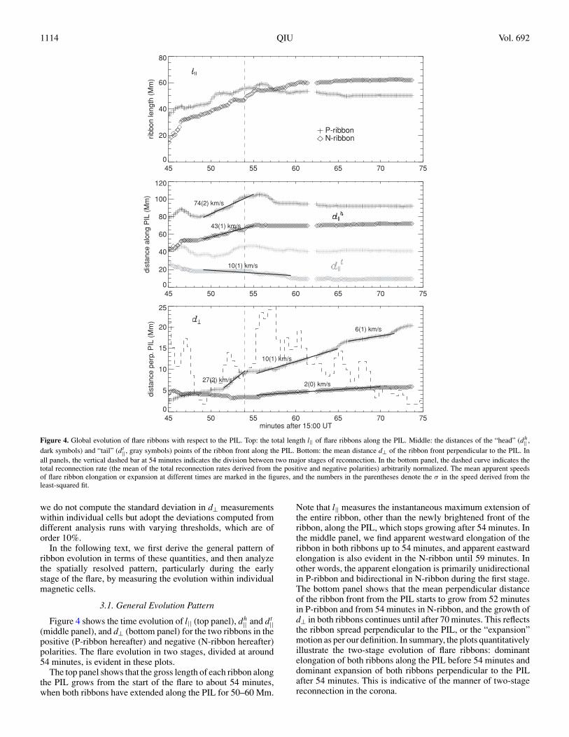
Figure 4. Global evolution of flare ribbons with respect to the PIL. Top: the total length l|| of flare ribbons along the PIL. Middle: the distances of the “head” (dh|| ,

dark symbols) and “tail” (dt||, gray symbols) points of the ribbon front along the PIL. Bottom: the mean distance d⊥ of the ribbon front perpendicular to the PIL. In

all panels, the vertical dashed bar at 54 minutes indicates the division between two major stages of reconnection. In the bottom panel, the dashed curve indicates thetotal reconnection rate (the mean of the total reconnection rates derived from the positive and negative polarities) arbitrarily normalized. The mean apparent speedsof flare ribbon elongation or expansion at different times are marked in the figures, and the numbers in the parentheses denote the σ in the speed derived from theleast-squared fit.

we do not compute the standard deviation in d⊥ measurementswithin individual cells but adopt the deviations computed fromdifferent analysis runs with varying thresholds, which are oforder 10%.

In the following text, we first derive the general pattern ofribbon evolution in terms of these quantities, and then analyzethe spatially resolved pattern, particularly during the earlystage of the flare, by measuring the evolution within individualmagnetic cells.

3.1. General Evolution Pattern

Figure 4 shows the time evolution of l|| (top panel), dh|| and dt

||(middle panel), and d⊥ (bottom panel) for the two ribbons in thepositive (P-ribbon hereafter) and negative (N-ribbon hereafter)polarities. The flare evolution in two stages, divided at around54 minutes, is evident in these plots.

The top panel shows that the gross length of each ribbon alongthe PIL grows from the start of the flare to about 54 minutes,when both ribbons have extended along the PIL for 50–60 Mm.

Note that l|| measures the instantaneous maximum extension ofthe entire ribbon, other than the newly brightened front of theribbon, along the PIL, which stops growing after 54 minutes. Inthe middle panel, we find apparent westward elongation of theribbon in both ribbons up to 54 minutes, and apparent eastwardelongation is also evident in the N-ribbon until 59 minutes. Inother words, the apparent elongation is primarily unidirectionalin P-ribbon and bidirectional in N-ribbon during the first stage.The bottom panel shows that the mean perpendicular distanceof the ribbon front from the PIL starts to grow from 52 minutesin P-ribbon and from 54 minutes in N-ribbon, and the growth ofd⊥ in both ribbons continues until after 70 minutes. This reflectsthe ribbon spread perpendicular to the PIL, or the “expansion”motion as per our definition. In summary, the plots quantitativelyillustrate the two-stage evolution of flare ribbons: dominantelongation of both ribbons along the PIL before 54 minutes anddominant expansion of both ribbons perpendicular to the PILafter 54 minutes. This is indicative of the manner of two-stagereconnection in the corona.

No. 2, 2009 OBSERVATIONAL ANALYSIS OF MAGNETIC RECONNECTION SEQUENCE 1115

We estimate the mean speed of the apparent ribbon spread inthe lower atmosphere by fitting time profiles of the measuredquantities as linear functions of time wherever appropriate. Fromthe top panel, the mean “growth” rate of the ribbon length upto 54 minutes amounts to 40 km s−1. From the middle panel,the apparent speed of the front along the PIL is 70 km s−1

for the P-ribbon, and 10–40 km s−1 for the N-ribbon, with afaster elongation to the west than to the east. From the bottompanel, we estimate the mean speed of apparent expansion forP-ribbon to be nearly 30 km s−1 from 52 minutes, reducingto 6–10 km s−1 after 54 minutes, and 2 km s−1 for N-ribbonfrom 54 minutes onward. When following certain locations offastest expansion along the ribbon, we measure the maximumexpansion speed up to 20 km s−1 in the N-ribbon, while along theP-ribbon, the perpendicular expansion is nearly homogeneousat all locations. Uncertainties, or deviations of different analysisruns and the fitting procedure, are of order 10% of the measuredmean speeds. The measured speeds of the apparent motionsare a fraction of, and at times maybe comparable with, thelocal Alfven speed, which is approximately 100–200 km s−1

in the lower atmosphere3 given an average plasma density of1012−14 cm−3 and magnetic field of 100–500 G in the activeregion. We also note that the flare ribbon in the positive polarityspreads, either parallel or perpendicular to the PIL, with a greaterspeed than in the negative polarity. This is a result of balancedmagnetic reconnection flux, as the negative ribbon resides instronger field, while the positive ribbon expands into weakerfields.

The apparent speed of ribbon elongation parallel to the PILin the lower atmosphere manifests the rate of reconnectionspreading along the assumed direction of the reconnectioncurrent sheet in the corona. The Alfven Mach number of theapparent speed in the corona Mc = Vc/Vca may be estimatedstarting with the flux conservation BcAc = BlAl , where Acis the area through which reconnecting field lines sweep inthe corona in a given instant, Al is the newly brightened areaswept by the flare in the lower atmosphere, and Bc and Blindicate magnetic field in the corona and lower atmosphere,respectively. We may approximate Ac and Al by Ac ≈ Vclcδtand Al ≈ Vlllδt , where V, l, and δt are the instantaneousapparent speed, a characteristic length perpendicular to V, anda given time interval during which reconnection takes place.Subscripts c and l indicate the parameters in the corona and loweratmosphere, respectively. Assuming that within a given instance,δt and l are identical in the corona and the chromosphere(as long as δt is longer than timescales of energy releaseand transfer), we arrive at Mc/Ml = (Vc/Vca)/(Vl/Vla) =(Bl/Bc × √

ρc)/(Bc/Bl × √ρl) = B2

l /B2c × √

ρc/ρl , whereρ is the plasma density. Order-of-magnitude, given the ratio ofthe magnetic field in the corona to the field in the chromosphere,and the ratio of plasmas density, it is seen that Mc/Ml ≈B2

l /B2c × √

ρc/ρl � 1. With the measured Ml ∼ 0.1–0.7, wetherefore arrive at Mc � 0.1–0.7. This is to say, the maximumapparent speed of reconnection spreading in the corona isnearly comparable to the coronal Alfven speed during the stageof parallel elongation, when the reconnection spreads nearlyalong the PIL. The measurements in this event observed at1600 Å are smaller than the speed measured by Kitahara &Kurokawa (1990) studying observations at Hα line center, butlarger than the apparent speed measured by Fletcher et al.

3 With respect to the 1600 Å UV continuum radiation, the lower atmospherewould refer to the chromosphere and below down to the temperature minimumregion.

(2004), who also studied observations in the 1600 Å UVcontinuum. However, for purposes different from this study,Fletcher et al. (2004) made the measurements by identifyingand following individual kernels, while in our measurementswe track the emitting features above a designated threshold atthe two ends of the ribbon along the PIL. The measured speedof the “head” and “tail” along the ribbon yields an estimate of“spread” of reconnection along the PIL, and is not necessarilythe apparent speed of a coherent kernel by Fletcher et al.(2004). Note that these parallel speeds measured in this paperand by Fletcher et al. (2004) are not chromospheric projectionof the reconnection inflow speed, but may be viewed as therate of perturbation propagation, the physical mechanism forwhich remains unknown, along the presumed direction of thereconnection current sheet. On the other hand, the speed of theapparent expansion perpendicular to the PIL may be interpretedas the projection of the coronal inflow speed, which makes anappreciable fraction of the Alfven speed (Mc � Ml ∼ 0.1 at themaximum in this event).

Our analysis reveals “unzipping” of magnetic reconnectionalong the PIL before the perpendicular expansion predominates.The same or similar phenomena have been reported in previousstudies. Apart from the traditional Hα observations of flareribbons (Kitahara & Kurokawa 1990; Moore et al. 2001), Suet al. (2007) showed the bright points observed by TRACE withan initial trajectory more parallel than perpendicular to the PIL.Krucker et al. (2005), Liu et al. (2006), Des Jardins (2007),and Grigis & Benz (2008) showed the parallel motion of hardX-ray footpoints along the PIL using RHESSI observations.These later observations, particularly hard X-ray observations,however, focus on localized sites of the strongest emission,presumably the sites of strongest energy release, whereas ouranalysis with an emphasis on reconnection sequence takesinformation of the entire ribbon by analyzing all the radiationenhancement produced by reconnection energy release.

3.2. Spatially Resolved Evolution

The above analysis yields the general pattern of flare ribbonevolution, by treating each of the two ribbons as a continuouslyextended patch. Examining the TRACE flare movie, we note thatat the start of the flare, brightenings took place at a few spatiallyseparated kernels. From 44 to 49 minutes, the spread of flarebrightenings along the ribbons is less in order, and is dominatedby the brightening filling up the gaps between bright kernels.The elongation pattern became organized, or directional, after49 minutes. To study these details in the initial stage of the flare,we analyze the spatially resolved evolution by measuring d|| andd⊥ in each of the magnetic cells.

Figure 5 shows time profiles of d|| and d⊥ for six majorcells, P3, P5, and P4, in the positive fields, and N1, N2,and N3, in the negative fields. Vertical bars on each curveindicate measurement uncertainties. Since the length of theribbon front in each cell is very small, we do not computethe standard deviation of d⊥ measurements at each time. Asthe primary purpose is to study spatial evolution particularlyduring the early stage, we do not present analysis in other cells,except P4, involved at later times. Also note that even thoughbrightening in the cell P7 occurs at the start of the flare, theflare kernel in P7 rapidly increases in area within 2–3 minutesand does not exhibit a clear pattern of elongation or expansion.Therefore, measurements in P7 are not presented. In each plot,the elongation (in both directions) and expansion of the flarebrightening are captured for each cell. These plots show that,

1116 QIU Vol. 692

P3

45 50 55 60 65 70 75

0

20

40

60

80

100P5

45 50 55 60 65 70 75

0

20

40

60

80

100P4

45 50 55 60 65 70 75

0

20

40

60

80

100

N3

45 50 55 60 65 70 75

0

20

40

60

80N1

45 50 55 60 65 70 75

0

20

40

60

80N2

45 50 55 60 65 70 75

0

20

40

60

80dis

tance (

Mm

)

minutes after 15:00 UT

Figure 5. Spatially resolved evolution of flare brightenings in magnetic cells. In each panel, the three curves from the top to the bottom show measurements (in unitsof Mm) of dh

|| , dt||, and d⊥, respectively, of the ribbon front in a major reconnection cell. Note that d⊥ is magnified by a factor of 2 for clarity. The vertical bars on the

curve indicate the measurement uncertainty. In each panel, the thin solid curve shows the reconnection rate in the cell in units of 1017 Mx s−1.

though less pronounced, the two-stage reconnection is reflectedin individual cells as well. In most cells, elongation along thePIL is prominent between 49 and 54 minutes, and perpendicularexpansion dominates afterward.

The figure also reveals a few details during the first stage,which are not seen in the global pattern. First, at the onset,brightenings started impulsively and simultaneously (within thecadence of the observation) at a few separate sites in differentcells, P3, P5, the boundary of N1 and N2, and also in the middleof N3 two minutes later. The approximate size of the kernelmay be estimated from the distance between the “head” and“tail” at the first time frame. The kernel inside P5 is piece-like, of 10 Mm, or about 7 MDI pixels. Some other kernelsare close to point sources (with the size comparable to theinstrument resolution). Second, the figure shows a precursorepisode from 44 to 49 minutes, when all individual kernelsare both elongating and expanding, filling up gaps betweenseparate kernels into a continuous piece of flare ribbon, whichthen elongates along both the western and eastern directions.Note that in this precursor episode when brightening starts inthe UV-1600 Å continuum, no enhancement in the GOES X-rayemission is observed. From 49 to 54 minutes, the cell P3 exhibitsan elongation motion eastward, while P5 primarily elongateswestward. In the negative polarity, N3 elongates bidirectionally.N1 elongates westward and N2 elongates eastward, both froma middle point between N1 and N2. The spatially resolvedanalysis yields speeds of the apparent expansion comparablewith the values derived for the global pattern. The apparentelongation speed within individual cells is somewhat smallerthan the maximum elongation speed seen in Figure 4, becausethe global elongation includes brightenings successively acrossadjacent cells, particularly along the PIL from P5 to P9 and P6.

4. RECONNECTION SEQUENCE ANALYSIS

The quantitative approach to determine the reconnection se-quence is through a correlation analysis between reconnection

rates derived in individual magnetic cells determined from parti-tioning in Figure 2. In principle, within a given interval, energyrelease takes place simultaneously at conjugate footpoints ofmagnetic field lines that are reconnecting. Therefore, the recon-nection fluxes at these sites evolve along with each other withbalanced positive and negative fluxes. With this principle, wedevelop an approach to pick out pairs of magnetic cells that arereconnecting within a given interval.

We denote the time profile of the reconnection rate of apositive cell during a given time interval as Φp(t, t + Δt), where pis from 1 to Np, Np being the number of positive cells, and denotethat of a negative cell during the same interval as Φn(t, t + Δt),where n is from 1 to Nn, Nn being the number of negativecells. Note that Φp and Φn are reconnection rates, or the timederivative of reconnection flux in the cells, derived from theequation in Section 1 and are not normalized to their maxima. IfΦp(t, t + Δt) and Φn(t, t + Δt) are correlated with a significantcross-correlation coefficient (e.g., greater than 0.5), these twomagnetic cells p and n are considered to be reconnecting duringthis interval from t to t + Δt . In practice, most magnetic cellsare involved in magnetic reconnection with multiple cells atmultiple times with different start and end times. If we divide theentire duration of the flare into intervals with fixed start and endtimes by any means and perform cross-correlation during theseintervals, we would miss out a significant number of peaks thatspan two fixed intervals. Therefore, we devise running intervalswith a fixed length of Δt = 5 minutes (10 time bins) suchthat the first interval starts from the time bin 1 and ends attime bin 10, the second interval starts from time bin 2 andends at 11, and so forth, and cross-correlate Φp(ti , ti + Δt) andΦn(ti , ti + Δt) for any set of p and n over i = 1, Nt − 9, whereNt is the total number of time bins. The length of the intervalshould be chosen in such a way that any single reconnectionpeak can be covered within a certain interval, while any giveninterval does not include more than one reconnection peak.Noting that the typical duration of an individual reconnection

No. 2, 2009 OBSERVATIONAL ANALYSIS OF MAGNETIC RECONNECTION SEQUENCE 1117

45 50 55 60 65 70 75

0.5

0.6

0.7

0.8

0.9

1.0

P7-N3P3-N3P5-N3P6-N3

45 50 55 60 65 70 75

0.5

0.6

0.7

0.8

0.9

1.0

P7-N1P3-N1P5-N1P6-N1

45 50 55 60 65 70 75

0.5

0.6

0.7

0.8

0.9

1.0

P7-N2P3-N2P5-N2P6-N2

minutes after 15:00 UT

corr

ela

tion c

oeffic

ient

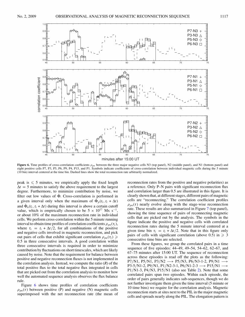
Figure 6. Time profiles of cross-correlation coefficients ρpn between the three major negative cells N3 (top panel), N2 (middle panel), and N1 (bottom panel) andeight positive cells P7, P3, P5, P6, P9, P4, P15, and P1. Symbols indicate coefficients of cross-correlation between individual magnetic cells during the 5 minute(10 bin) interval centered at the time bin. Dashed lines show the total reconnection rate arbitrarily normalized.

peak is � 5 minutes, we empirically apply the fixed lengthΔt = 5 minutes to satisfy the above requirement to the largestdegree. Furthermore, to minimize contribution by noise, wefilter out low values of Φ. Cross-correlation is performed ina given interval only when the maximum of Φp(ti , ti + Δt)and Φn(ti , ti + Δt) during this interval is above a certain cutoffvalue, which is empirically chosen to be 5 × 1017 Mx s−1,or about 10% of the maximum reconnection rate in individualcells. We perform cross-correlation within the 5 minute runninginterval to obtain time profiles of correlation coefficients ρpn(τi),where τi = ti + Δt/2, for all combinations of the positiveand negative cells involved in magnetic reconnection, and pickout pairs of cells that exhibit significant correlation ρpn(τi) �0.5 in three consecutive intervals. A good correlation withinthree consecutive intervals is required in order to minimizecontribution by fluctuations on short timescales, which are likelycaused by noise. Note that the requirement for balance betweenpositive and negative reconnection fluxes is not implemented inthe correlation analysis. Instead, we compute the ratio (R) of thetotal positive flux to the total negative flux integrated in cellsthat are picked out from the correlation analysis to monitor howwell the automated sequence analysis observes the flux balancerule.

Figure 6 shows time profiles of correlation coefficientsρpn(τ ) between positive (P) and negative (N) magnetic cellssuperimposed with the net reconnection rate (the mean of

reconnection rates from the positive and negative polarities) asa reference. Only P–N pairs with significant reconnection fluxand correlation larger than 0.5 are illustrated in this figure. It isclearly shown that, at different stages, different pairs of magneticcells are “reconnecting.” The correlation coefficient profilesρpn(τ ) nearly evolve along with the stage-wise reconnectionrate. These results are also summarized in Figure 7 (top panel),showing the time sequence of pairs of reconnecting magneticcells that are picked out by the analysis. The symbols in thefigure indicate the positive and negative cells with correlatedreconnection rates during the 5 minute interval centered at agiven time bin τi = ti + Δt/2. Note that in this figure onlypairs of cells with significant correlation (above 0.5) in � 3consecutive time bins are selected.

From these figures, we group the correlated pairs in a timesequence of five episodes: 44–49, 49–54, 54–62, 62–67, and67–75 minutes after 15:00 UT. The sequence of reconnectionacross these episodes is read off the plots as the following:P7/N1, P5/N1, P3/N2 −→ P5/N3, P6/N3-1-2, P9/N1 −→P3-5/N1-2, P9/N1, P1/N2-3-1, P6/N1-2-3 −→ P15/N1 −→P1/N1-3, P4/N3, P15/N1 (also see Table 2). Note that somecorrelated pairs span two episodes. Within each episode, theorder of pairs generally indicates sub-sequences, though we donot further investigate them given the time interval (5 minute or10 time bins) we require for the correlation analysis. Magneticreconnection starts at sites next to the PIL in the major magneticcells and spreads nearly along the PIL. The elongation pattern is

1118 QIU Vol. 692

45 50 55 60 65 70 75

0.5

0.6

0.7

0.8

0.9

1.0

P9-N3P4-N3P15-N3P1-N3

45 50 55 60 65 70 75

0.5

0.6

0.7

0.8

0.9

1.0

P9-N1P4-N1P15-N1P1-N1

45 50 55 60 65 70 75

0.5

0.6

0.7

0.8

0.9

1.0

P9-N2P4-N2P15-N2P1-N2

minutes after 15:00 UT

corr

ela

tion c

oeffic

ient

Figure 6. (Continued)

most evident from 49 to 54 minutes. Seen from Figure 2, in thenegative polarities, sequential reconnection occurs along N3,N1, and N2, and in the positive polarities, the spreading alongthe PIL takes place in P7, P3, and P5, and then reconnectioninvolves cells P9 and P6 in the western portion of the activeregion. Magnetic reconnection during the first stage plays therole of forming the skeleton of two ribbons along the PIL innearly a sequential manner. Into the second stage, a greaternumber of magnetic cells are participating in reconnection. Inthe positive polarity, reconnection involving P3 and P5 proceedsinto P4 and P15, both further away from the PIL, and in thenegative polarity, reconnection proceeds within N3 and N1, indirections nearly perpendicular to the local PIL. Ultimately,reconnection sequence ends at P4, P15, N1, and N3 in the coreregion, as well as P1 in the western portion.

The reconnection sequence analysis is able to produce amajor reconnection sequence characterizing how individualmagnetic cells participate in reconnection. This result indicatesthat magnetic reconnection in the corona, on the one hand,does not exhibit a smooth and continuous evolution, and on theother hand, is not entirely chaotic. That magnetic reconnectionproceeds sequentially, but not smoothly, between individualmagnetic cells is most pronounced in Figure 7 (top panel),which reveals different pairs of magnetic cells picked out bythe correlation analysis at different episodes (or peaks). Thedistinctive patterns are evident not only between the two stages,the parallel elongation and the perpendicular expansion, but alsoduring different episodes on shorter timescales. For example,during expansions from P5 to P15, the rise of the reconnectionrate around 64 min is coincident with reconnection penetratinginto the strong field region of P15. Similarly, reconnection peaksaround 67 minutes are coincident with expansion from P3 to P4and from N2 into N8. Note that most peaks in reconnection

rates are registered in a few magnetic cells in both polarities,therefore, these peaks are a reflection of the coronal processrather than artifacts of analyzing highly structured photosphericmagnetograms.

We note that the reconnection sequence analysis is a first-order approach, as we spatially resolve the reconnection rateon scales of individual flux cells other than at pixel level andtemporally resolve reconnection on 1 minute timescale, whichis much longer than the observing cadence of 2 s. This issensible, because below these macroscopic scales, the natureof reconnection is perhaps more sporadic than ordered. It isnoted that even at the present temporal-spatial scales, all cells inreconnection cannot be picked up by the correlation analysis. Forexample, early in the second episode (49–54 minutes), judgedfrom Φ time profiles, P9 and N3 are likely correlated hencereconnecting ahead of P6/N3, but the P9/N3 pair is not selectedby the automatic analysis procedure because Φ in P9 is lowerthan the low cutoff value of 5×1017 Mx s−1. Because of very lowΦ, N8 and N12 are also discarded in the correlation analysis,though they participate in reconnection after 60 minutes. Tohave a sense of how well the correlation analysis works, wesum up reconnection flux in all the correlated pairs picked upby the automated analysis and derive the fraction of correlatedflux to the total reconnection flux at given time bins as shownin Figure 7 (bottom panel) as well as in Table 1.4 It is foundthat on average over three quarters of the total reconnectionflux is picked by the correlation analysis, and the remainder is

4 Note that the total correlated flux in each episode is computed differently inTable 1 and in Figure 7 (bottom panel): in the table, only reconnection flux ineach episode is computed, and in the figure, at each point, the values ofreconnected flux and flux ratio are computed from integral over the 5 minutebox centered at the given time bin.

No. 2, 2009 OBSERVATIONAL ANALYSIS OF MAGNETIC RECONNECTION SEQUENCE 1119

Table 1Reconnection Sequence

Episodes 44–49 49–54 54–62 62–67 67–75(Minutes After 15:00 UT)

Correlated Pairs P7/N1 P5/N1a P3/N1-2 P6/N3-2a P1/N1-3P5/N1 P3/N2a P5/N1-2 P1/N3-1-2a P4/N3P3/N2 P5/N3 P9/N1 P15/N1 P15/N1

P6/N3-1-2 P1/N2-3-1P9/N1 P6/N1-2-3

Total Reconnection Fluxb 1.21/0.69 0.74/0.75 2.04/2.06 1.09/1.03 0.80/0.45Flux Ratio (P/N) 1.77 0.99 0.99 1.07 1.78Total Correlated Fluxb,c 1.21/0.65 0.57/0.69 1.92/2.00 0.75/0.97 0.75/0.31Flux Ratio (P/N)c 1.87 0.83 0.96 0.77 2.43

Notes.a This correlated pair is apparently continued from the previous episode.b The reconnection flux is in units of 1021 Mx, and the numbers before and after the “/” indicate fluxes in the positive and negativepolarities, respectively.c The reconnection flux is calculated for each episode without taking into account the 5 minute box applied in the correlation analysis,different from Figure 7 (bottom panel).

Table 2Reconnection Fluxa

Positive Cells P1 P3 P4 P5 P6 P7 P9 P15

Total Magnetic Flux (1021 Mx) 6.8 1.7 2.2 1.1 1.2 0.3 0.5 0.8Obs. Reconnection Flux (1021 Mx) 1.2 1.5 0.3 1.0 0.5 0.0 0.2 0.3Model Reconnection Fluxb (1021 Mx) 0.61 0.89 0.47 0.88 · · · · · · · · · 0.24Total Reconnection Flux (Fraction) 18% 89% 13% 87% 38% 6% 33% 39%Reconnection Flux in First Stage 0% 47% 0% 47% 10% 6% 2% 3%Reconnection Flux in Second Stage 18% 42% 13% 40% 28% 0% 31% 36%

Negative Cells N1 N2 N3 N7 N8 N12

Total Magnetic Flux (1021 Mx) 5.3 3.1 2.5 1.8 0.9 0.5Obs. Reconnection Flux (1021 Mx) 1.5 1.4 1.5 0.0 0.1 0.0Model Reconnection Fluxb (1021 Mx) 1.43 0.50 1.19 0.34 · · · · · ·Total Reconnection Flux (Fraction) 29% 46% 61% 2% 13% 7%Reconnection Flux in First Stage 9% 8% 16% 1% 0% 0%Reconnection Flux in Second Stage 20% 38% 45% 1% 13% 7%

Notes.a Unless indicated, the reconnection fluxes listed in the table refers to observationally measured fluxes.b The model predicted reconnection flux in a given cell is computed from Table 1 in Longcope et al. (2007) by averaging all thefluxes donated (ΔΨ↓ in their paper) and received (ΔΨ↑) by this cell.

not apparently correlated. In the same plot, we also show theratio of positive to negative flux from correlated cells. The fluxratio usually deviates from unity but the median value comesclose to unity and within the range of uncertainties (see Qiuet al. 2007). When broken down into the five episodes, asshown in Table 1, it is seen that there is relatively larger fluximbalance in the first and last episodes, which may be caused bythe low reconnection rate leading to inaccurate estimates. Theabove analysis provides a qualitative measure of how well thesequence analysis works. Both physical and unphysical reasonscontribute to the flux imbalance. Unphysical reasons includeuncertainties in both the reconnection flux measurements fromflare signatures and the partitioning of the magnetogram, andthe limitation of the present method of correlation analysis.Physically, although our analysis with the presently designatedtemporal and spatial scales captures the major reconnectionsequence faithfully, on fine scales, magnetic reconnection mayproceed in a more complex manner than following a single majorsequence.

Magnetic reconnection is thought to relax the pre-reconnection magnetic field to a low-energy configuration by al-

lowing flux exchanges between magnetic domains. The amountsof flux exchange, or reconnection fluxes, between magnetic cellsare measured from observations. Observations reveal that eachof most magnetic cells does not participate in magnetic recon-nection by its entirety. Table 2 lists the amount of reconnectionflux as a fraction of the total flux in each magnetic cell. In themajor cells P3, P5, N3, and N2, reconnection flux makes closeto or more than half of the total flux, while in other cells, re-connection flux is less than half of the total flux. Also given inthe table is the amount of reconnection flux during two stagesdivided at 54 minutes. For comparison, we also compute themodel predicted reconnection flux by Longcope et al. (2007).The predicted reconnection flux in each cell is the mean ofthe total received flux Δψ↑ and total donated flux Δψ↓ (in ab-solute values) in this cell. The observational measurements ofreconnection flux presented here are systematically larger thanthe numbers from the model prediction, because in this paperwe use the photospheric magnetogram without extrapolation tohigher altitudes, and a lower threshold for the flare radiation andno frame integration to emphasize weak features. These differ-ent steps can raise the measured reconnection flux by about

1120 QIU Vol. 692

45 50 55 60 65 70 75

minutes after 15:00 UT

N 1N 2N 3N 5N 7N 8

P 1P 3P 4P 5P 6P 7P 9P15

(a)

45 50 55 60 65 70 75minutes after 15:00 UT

0.1

1.0

10.0

fraction of correlated flux out of totalratio of positive to negative flux

(b)

Figure 7. Summary plot of reconnection sequence. (a): the time evolution ofconnectivity. Symbols indicate magnetic cells whose reconnection rates arecorrelated with cells in opposite polarities within a 5 minute box centered at thetimes. The curves indicate the net reconnection rate derived in the positive (thicksolid line) and negative (thin solid line) polarities, respectively, normalized toarbitrary units. (b): net reconnection flux summed over all the correlated cellsas a fraction of the total reconnection flux (diamond symbols), and the ratio ofpositive to negative flux in reconnecting cells (plus symbols). In both panels,solid bars indicate five episodes of reconnection, and the thick solid bar at 54minutes indicates the division of two major reconnection stages.

20%–30%, but do not affect the evolution pattern of recon-nection flux and reconnection rate. Minor details may changewhen different sets of parameters are applied in the correlationanalysis. However, our experiments show that these variationswould not significantly modify the major reconnection sequenceshown in the foregoing text. Such analysis, though with ampleroom for improvement, makes it possible to start comparing andbridging observations and models in order to uncover the truethree-dimensional topology of magnetic reconnection. A briefdiscussion of the model–observation comparison will be givenin Section 5.

5. DISCUSSIONS

5.1. Three-Dimensional Evolution of Magnetic Reconnection

Results from the above two sections may be combined toarrive at a picture of the three-dimensional evolution of connec-tivity between magnetic cells. Figure 8 shows the sketch of thereconnection sequence at each given episode as determined fromthe reconnection sequence analysis (see Table 1). In the figure,the pairs of major reconnecting cells determined from correla-

tion analysis are connected by dashed lines, and the arrow oneach cell indicates the direction of the spread within the cell.As the reconnection sequence alone cannot distinguish the pre-reconnection and post-reconnection connectivities, we assumethat the correlation pattern, which is obtained by employing ra-diation signatures, indicates the post-reconnection connectivity.In other words, the correlated pairs of cells are considered to befeet of postflare loops.

In this context, it is seen that in the precursor episode ar-cades of postflare loops are formed in a sequence. Formationof loops connecting P5 and N1 spreads to the west, and for-mation of loops connecting P3 and N2 spreads to the east,suggestive of “unzipping” of magnetic reconnection along theaxis of low-lying arcade. Note that these low-lying loops in-ferred from the correlation analysis would be sheared with re-spect to the PIL. The pattern of connectivity changes sharplyfrom 49 to 54 minutes, when we see a rapid westward elon-gation along P5–P9–P6 in the positive polarity, and meanwhilean eastward elongation from N3 to N1 and then N2, result-ing in the connectivity of P5/N3, P9/N3-1, and P6/N3-1-2.Note that this is also the stage with the most rapid elonga-tion primarily along the PIL, with the apparent speed at timeslarger than 100 km s−1, comparable to the local Alfven speed.If the inferred connectivity refers to the post-reconnection con-nectivity, this stage would characterize the formation of longloops connecting P9/N3-15 and P6/N3-1-2, which are nearlyparallel to the PIL, together with shorter loops connectingP5 and N3, which are more perpendicular to the PIL. After54 minutes, the connectivity pattern would indicate the for-mation of loops connecting the outer edges of P3 (extended toP4), P5 (extended to P15) and N1–N3, as well as P1 and N-cells,which are more perpendicular to the PIL. In summary, the recon-nection sequence suggests the following three-dimensional evo-lution of magnetic reconnection: the formation of short shearedlow-lying loops, the formation of long loops nearly parallel tothe PIL, and the formation of overlying loops more perpendic-ular to the PIL.

Change of connectivities between source magnetic cells bymagnetic reconnection carries along helicity transfer betweendifferent magnetic structures. One plausible consequence of thehelicity transfer is the formation of a flux rope by convertingthe mutual helicity of sheared pre-flare loops to the self-helicity(twist) of the rope (van Ballegooijen & Martens 1989; Longcopeet al. 2007). The reconnection sequence (particularly during theelongation) from above analysis implies such a likely scenario.Hypothetically, during the stage of rapid directional elongation,the formation of long loops would make the axis of the posteriorflux rope, and reconnection in the ensuing expansion stage addstwists to the flux rope. The sequence analysis suggests that P1and N1 or N3 might become the feet of the rope. The totalreconnected flux in P1 and N3 would set an upper limit ofthe rope flux, which is 1.2 to 1.5 × 1021 Mx. The poloidalflux of the rope (or the amount of twist), if in a simplifiedmanner conjectured by Moore et al. (2001), Longcope et al.(2007, Figure 1), Qiu et al. (2007), and Moore et al. (2007),would be very close to the arcade flux threading from P3/4-P5/15 to N1-2-3 formed by reconnection during the second(perpendicular expansion) stage, amounting to (3–4) ×1021 Mx.Therefore, the hypothetical flux rope has at least two to threeturns per unit length on average. The sense of the flux rope is

5 In the following text and Figure 8, we include the pair P9/N3 in the secondepisode from visual inspection of their Φ(t) profiles, though it is not picked outby the automated correlation analysis.

No. 2, 2009 OBSERVATIONAL ANALYSIS OF MAGNETIC RECONNECTION SEQUENCE 1121

P3 P5 P9 P6

P4 P15 P1

N3N1N2

P7

(a) pre-cursor (44 - 49 min)

P3 P5 P9 P6

P4 P15 P1

N3N1N2

P7

(b) elongation (49 - 54 min)

P3 P5 P9 P6

P4 P15 P1

N3N1N2

P7

(c) expansion (54 - 67 min)

P3 P5 P9 P6

P4 P15 P1

N3N1N2

P7

(d) decay (after 67 min)

Figure 8. Sketch of connectivities between magnetic cells and evolution of cell brightening with respect to PIL during the flare. In each panel, circles give therelative positions of major magnetic cells that participate in reconnection and the dotted line marks the PIL. Dashed lines connect positive and negative cells that arereconnecting at a given episode as determined from the sequence analysis. Arrows give the direction of the spread of brightening in the cell with respect to the PIL.

left handed, same as the interplanetary flux rope manifested as aMagnetic Cloud (Longcope et al. 2007). Rigorous computationof the helicity transfer and amount of twist in a full three-dimensional approach, however, has to occur only when the priorconnectivity is known or modeled. The reconnection sequenceanalysis alone cannot answer this question. A preconnectiontopological structure of the corona has to be given, such as inLongcope et al. (2007).

With the notion above, we briefly discuss how the observa-tionally inferred reconnection sequence compares with predic-tions from the topological model (Longcope et al. 2007). Bothagreement and discrepancies are found between the two inde-pendently determined sequences. The topology model predictsthe following sequence in the positive polarity P5−→P15−→P13−→P8−→P4, and in the negative polarity, the sequencefollows along N3−→N1−→N2. In comparison with observa-tional measurements, the topological model captures the gen-eral direction along which flare ribbons form, particularly in thenegative polarity, though it does not distinguish the two-stagereconnection within individual cells as revealed in observations.Effectively, the topological model combines the two stages, theparallel and perpendicular expansions, observed in the flare evo-lution into one. It remains to be investigated what is the physi-cal implication of the observed two-stage evolution to topologicmodels of reconnection. Quantitatively, the model is able to in-clude most magnetic cells that are involved in reconnection asrevealed by flare observations, and the computed reconnectionflux in each cell is comparable with observational measurementsfor the majority of reconnecting cells. As illustrated in Table 2,the model captures five cells (out of the observed eight) in thepositive polarity, and four cells (out of the observed six) in thenegative polarity. Given that the observational measurements inthis paper are the upper limits of the range of values, we mayconsider that the reconnection fluxes from model computationand from observational measurements are consistent and closelycomparable in three major positive cells (P3, P5, P15) and twomajor negative cells (N1 and N3), with minor discrepancies wellwithin the range of uncertainties in measuring the reconnectionflux from observations as well as determining connectivities inthe model. Other discrepancies include the following: in the

positive polarity, the model does not consider P6 and P9, andoverestimates the flux in P4, P2, and P13 in comparison withobservations; in the negative polarity, the model underestimatesthe flux in N2 and overestimates the flux in N7 and N10. How-ever, it is noted that the contribution of reconnection flux bythese significantly mismatched cells is small, which makes up to30% of the total reconnection flux. This though very crude first-order comparison shows a good degree of agreement betweenentirely independent determinations of reconnection fluxes inindividual cells given uncertainties in both methods, which maysuggest that the model reasonably represents the observed evo-lution of reconnection, and, therefore, the change to the helicityand energy estimates by adjusting the model to better reproduceobservations may be expected to be minor. In an ensuing study,we will conduct detailed comparisons between the model andobservation and discuss the implication of the comparison.

5.2. Energy Release

Reconnection releases energy by converting free magneticenergy into heating plasmas and accelerating charged particlesas well as bulk plasmas. The rate of energy release is governed bymacroscopic corona field configuration and microscopic physicsof magnetic reconnection. Among important physical quantitiescharacterizing magnetic reconnection, the macroscopic rateof magnetic reconnection may be inferred by employing theflux conservation principle as performed in this paper. Themacroscopic reconnection rate is equivalent to the inducedelectric field (Ec) integrated along the length of the current sheet,and the work done by this field on the current is equivalent tothe amount of energy release by magnetic reconnection in thecorona. Our knowledge of this other key parameter, current (Ic)or the effective resistivity (ηc), has been largely a matter ofguess.

To make a step closer to understanding energy release, weprobe the relation of the energy release rate to the reconnectionrate so as to shed light on this critical but hardly measurableparameter. Existing observing facilities cannot yield a directmeasurement of the total energy released by reconnection duringa flare, and in this discussion, we only employ an estimate ofthermal energy as an approximation to flare energy release.

1122 QIU Vol. 692

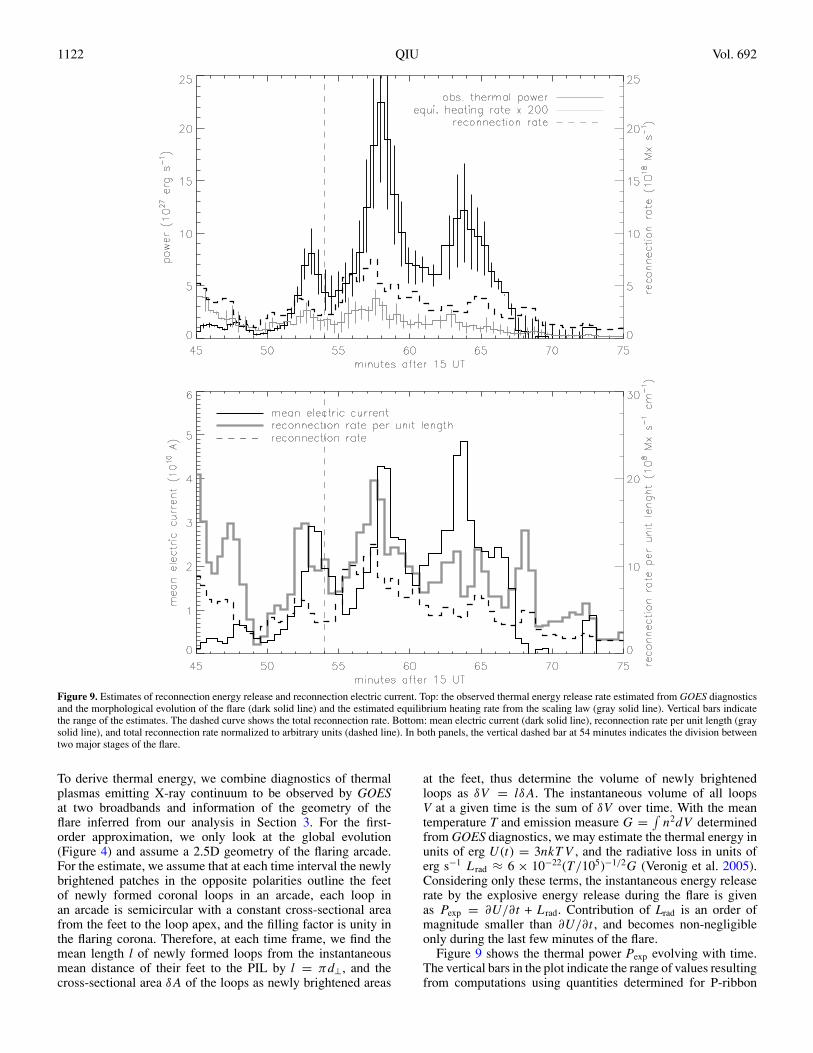
Figure 9. Estimates of reconnection energy release and reconnection electric current. Top: the observed thermal energy release rate estimated from GOES diagnosticsand the morphological evolution of the flare (dark solid line) and the estimated equilibrium heating rate from the scaling law (gray solid line). Vertical bars indicatethe range of the estimates. The dashed curve shows the total reconnection rate. Bottom: mean electric current (dark solid line), reconnection rate per unit length (graysolid line), and total reconnection rate normalized to arbitrary units (dashed line). In both panels, the vertical dashed bar at 54 minutes indicates the division betweentwo major stages of the flare.

To derive thermal energy, we combine diagnostics of thermalplasmas emitting X-ray continuum to be observed by GOESat two broadbands and information of the geometry of theflare inferred from our analysis in Section 3. For the first-order approximation, we only look at the global evolution(Figure 4) and assume a 2.5D geometry of the flaring arcade.For the estimate, we assume that at each time interval the newlybrightened patches in the opposite polarities outline the feetof newly formed coronal loops in an arcade, each loop inan arcade is semicircular with a constant cross-sectional areafrom the feet to the loop apex, and the filling factor is unity inthe flaring corona. Therefore, at each time frame, we find themean length l of newly formed loops from the instantaneousmean distance of their feet to the PIL by l = πd⊥, and thecross-sectional area δA of the loops as newly brightened areas

at the feet, thus determine the volume of newly brightenedloops as δV = lδA. The instantaneous volume of all loopsV at a given time is the sum of δV over time. With the meantemperature T and emission measure G = ∫

n2dV determinedfrom GOES diagnostics, we may estimate the thermal energy inunits of erg U (t) = 3nkT V , and the radiative loss in units oferg s−1 Lrad ≈ 6 × 10−22(T/105)−1/2G (Veronig et al. 2005).Considering only these terms, the instantaneous energy releaserate by the explosive energy release during the flare is givenas Pexp = ∂U/∂t + Lrad. Contribution of Lrad is an order ofmagnitude smaller than ∂U/∂t , and becomes non-negligibleonly during the last few minutes of the flare.

Figure 9 shows the thermal power Pexp evolving with time.The vertical bars in the plot indicate the range of values resultingfrom computations using quantities determined for P-ribbon

No. 2, 2009 OBSERVATIONAL ANALYSIS OF MAGNETIC RECONNECTION SEQUENCE 1123

and N-ribbon separately, and using a variety of temporal andspatial smoothing parameters. It is seen that Pexp is correlatedwith the reconnection rate with a 1–2 minute lag, as also seen,not surprisingly, in the direct time derivative of the GOES softX-ray light curve (Figure 3). The estimated Pexp includingonly those thermal energy terms is about 2 × 1028 erg s−1

at the peak, and the total thermal energy integrated over the20 minute duration of the flare amounts to 8 × 1030 erg. Theratio of the thermal energy release rate to the reconnection rateyields the mean instantaneous current Ic in the reconnectionregion, as shown in Figure 9 (bottom panel). It peaks at5 × 1010 A, and fluctuates during the flare. Note that despitean appreciable reconnection rate before 49 minutes the energyrelease rate is very low. This may suggest that the effectivecurrent is very small during the precursor stage when ribbons areimpulsively “filling up,” or it may be caused by a delay of plasmaheating and radiation at GOES temperature. For this flare, hardX-ray observations by RHESSI missed the impulsive phase, sowe cannot verify whether significant instantaneous nonthermalenergy release takes place at the precursor. The mean effectiveresistivity along the length of the current sheet is estimated tobe ηc = Φ2/Pexpl|| ≈ 10−7 Ω m−1, where Φ is the reconnectionrate.

To compare the explosive energy release via magnetic re-connection during flares with other steady-state situations,we also estimate the heating rate of coronal loops in hydro-static equilibrium, using the geometric quantities inferred inSection 3 and the scaling law given by Schrijver et al. (2004):Pequ = ∂E/∂t = 1.4 × 1014B/llA. The scaling law is derivedfrom nonflaring long-lived coronal loops in active regions. Inthis relation, B is the magnetic field strength at the (chromo-sphere) feet of the loops, which is measured, in this paper, asthe mean magnetic field encompassed by newly brightened rib-bons. The time profile of Pequ is plotted in Figure 9. It is nosurprise that Pequ is smaller than the observed explosive en-ergy release rate Pexp by nearly 3 orders of magnitude, as thescaling law describes the corona heated in a steady-state process(Schrijver et al. 2004). Comparison between Pequ and Pexp yieldsthat the effective resistivity or current during the explosive en-ergy release is raised by 3 orders of magnitudes.

Note that the above estimate of the energy release ratehas to deal with some assumptions, that energy released inreconnection is primarily (or ultimately) converted into thermalenergy in arcades of semicircular loops, and that the coolingtimescales are significantly long so that all heated plasmas areseen by GOES throughout the flare and evolve isothermally. Inreality, during the early impulsive phase, flare loops are likelysheared as suggested by the sequence analysis in the foregoingsections, thus the current may be greater in the early phase thanshown in the figure with a semicircular assumption. The secondassumption of infinitely long cooling time puts our energyestimate as an upper limit of the thermal energy of plasmasdetected by GOES, because of the dependence Pexp ∼ √

V ,V being maximized by the infinite cooling time assumption.Furthermore, comparison of timings of the reconnection rateand the thermal energy release rate (Pexp) is meaningful onlywhen the effective timescale of plasma heating (so as to radiateat the GOES temperature) relative to the timescale of evolutionof magnetic reconnection (a few minutes) is understood. Theapparent lag of the energy release rate with respect to thereconnection rate may be interpreted as due to the interplayof both the reconnection rate and the reconnection current(or effective resistivity) when the timescale of plasma heating

is much shorter than the evolution timescale of magneticreconnection. Finally, the above discussion is confined to energyrelease by a nonideal resistive MHD process (reconnection),which is, presumably, ultimately converted to thermal energy.

In addition, Figure 9 (bottom panel) also shows the meanreconnection rate per unit length along the PIL to be of order(0.5–2)×109 Mx s−1 cm−1, equivalent to a mean electric fieldof 5–20 V cm−1 in the two-dimensional regime. Readers arereminded that although the figure shows an apparent peakof the reconnection rate per unit length at the precursor, itcannot be readily interpreted as the instantaneous reconnectionelectric field. The apparent motion of the flare ribbons before54 minutes is primarily parallel to the PIL, or along theassumed direction of the reconnection current sheet, thus theapparent speed is not equivalent to the reconnection inflowspeed as in the two-dimensional assumption. In general, thereconnection electric field Ec = VlBl has to be measuredwith caution. When the flare evolution cannot be depicted bya two-dimensional model, or the apparent spread cannot beconvincingly decomposed into a component perpendicular tothe direction of the reconnection electric current, determinationof VlBl is dubious if not meaningless.

6. CONCLUSIONS

We employ the reconnection sequence analysis to find thetemporal and spatial evolution of magnetic reconnection. Wepartition the photospheric magnetic field into individual cells,derive time profiles of the reconnection rate in these cells, andobtain the sequence of magnetic reconnection between thesecells from a correlation analysis. The method is applied to anX2.0 two-ribbon flare occurred on 2004 November 7, which ex-hibits several episodes of magnetic reconnection. It is seen thatthe method can pick up pairs of magnetic cells that are reconnect-ing during these episodes in a sequential manner. The analysisyields physical quantities directly comparable with topologicalmodels, thus is promising to provide observational constraintsto justify subsequent calculation of helicity transfer and energyrelease from the model. A brief model–observation comparisonfor one event in the present study shows reasonable agreementbetween independently determined physical quantities, thoughsome details differ and deserve further investigation.

The analysis also reveals two distinctive stages of magneticreconnection, namely, parallel elongation and perpendicularexpansion of flare ribbons with respect to the PIL. Elongationof flare ribbons along the PIL during the first stage proceedsat apparent maximum speeds comparable with the Alfvenspeed in the active region chromosphere, which may reflect thepropagation of perturbation in the corona along the reconnectioncurrent sheet. The apparent perpendicular expansion speed,reflecting the reconnection inflow in the corona, is a fraction(up to 10%) of the local Alfven speed. These two stagesare also marked in time profiles of the reconnection rate andenergy release. Although the elongation, or “unzipping” of flareribbons, has been reported in traditional flare observations (seeMoore et al. 2001, for the most comprehensive discussion) aswell as discovered lately in three-dimensional MHD simulationsof corona reconnection (Linton 2008), it remains unclear whatare the physical mechanisms governing the division of the twodistinctive stages of reconnection.

As the last remark, we note that the reconnection sequenceanalysis method has a few advantages. First, we directly exam-ine the temporal and spatial evolution of the reconnection ratein a quantitative manner, which is physically more meaningful

1124 QIU Vol. 692

than radiation signatures alone. Second, the method avoids somedifficulties in using the radiation signatures for quantitative anal-ysis, such as flat-fielding, nonlinear exposure treatment, seeingeffects in ground-based observations, and unknown intrinsicphysics such as cooling profiles of flaring atmosphere. Theseeffects would produce fluctuations and uncertainties in emis-sion signatures thus pose difficulty in interpreting their timeprofiles and correlation patterns. The reconnection sequenceanalysis only takes the message of the differential brighteningarea regardless of the intensity variations in the flaring region,thus avoiding all the above difficulties. The problem would oc-cur with spatial fluctuations in the magnetograms due to eitherphysical (such as evolution of magnetic fields) and unphysicalreasons. The method is useful to deal with timescales of or-der 30–60 s, which is a compromise between instrumental timeresolution and physical and unphysical conditions that requirea smoothing procedure before analyzing the time profiles. Theresult of our analysis on a flare event suggests that the analy-sis on such timescales as well as spatial scales prescribed bythe present partitioning method yields physically meaningfulmeasurements to provide observational constraints for models.

The author thanks Dana W. Longcope, Richard C. Canfield,and Ronald Moore for insightful discussions, and the referee forconstructively critical comments leading to significant improve-ment of the manuscript. I acknowledge TRACE and SOHO mis-sions for providing quality observations. This work is supportedby NSF grants ATM-0603789, ATM-0748428, and NASA grantNNX08AE44G.

REFERENCES

Barnes, G., Longcope, D. W., & Leka, K. D. 2005, ApJ, 629, 561Demoulin, P. 2006, AdSpR, 37, 1269Demoulin, P., Henoux, J. C., & Mandrini, C. H. 1992, Sol. Phys., 139, 105Demoulin, P., Henoux, J. C., & Mandrini, C. H. 1994, A&A, 285, 1023Des Jardins, A. C. 2007, PhD thesis, Montana State Univ.Fletcher, L., & Hudson, H. 2001, Sol. Phys., 204, 69Fletcher, L., Pollock, J. A., & Potts, H. E. 2004, Sol. Phys., 222, 279

Forbes, T. G., & Priest, E. R. 1984, in Solar Terrestrial Physics: Present andFuture, ed. D. M. Butler & K. Paradupoulous (NASA), 1

Grigis, P. C., & Benz, A. O. 2008, SPD/AGU, SP 44A-05, Fort Lauderdale,Florida

Handy, B. N., et al. 1999, Sol. Phys., 187, 229Isobe, H., Takasaki, H., & Shibata, K. 2005, ApJ, 632, 1184Isobe, H., Yokoyama, T., Shimojo, M., Morimoto, T., Kozu, H., Eto, S.,

Narugake, N., & Shibata, K. 2002, ApJ, 566, 528Kawaguchi, I., Kurokawa, H., Funakoshi, Y., & Nakai, Y. 1982, Sol. Phys., 78,

101Kitahara, T., & Kurokawa, H. 1990, Sol. Phys., 125, 321Krucker, S., Fivian, M. D., & Lin, R. P. 2005, Adv. Space Res., 35, 1707Linton, M. G. 2008, SPD/Karen Harvey Prize Lecture, SPD/AGU, SP 42A-01,

Fort Lauderdale, FloridaLiu, C., Lee, J., Deng, N., Gary, D. E., & Wang, H. 2006, ApJ, 642, 1205Longcope, D. W. 1996, Sol. Phys., 169, 91Longcope, D. W., Barnes, G., & Beveridge, C. 2009, ApJ, in pressLongcope, D. W., & Beveridge, C. 2007, ApJ, 669, L621Longcope, D. W., Beveridge, C., Qiu, J., Ravindra, B., Barnes, G., & Dasso, S.

2007, Sol. Phys., 244, 45Moore, R. L., & La Bonte, B. J. 1980, Proc. Symp., Solar and Interplanetary

Dynamics (Dordrecht: Reidel), 207Moore, R. L., Sterling, A. C., Hudson, H. S., & Lemen, J. R. 2001, ApJ, 552,

833Moore, R. L., Sterling, A. C., & Suess, S. T. 2007, ApJ, 668, 1221Neupert, W. M. 1968, ApJ, 153, L59Poletto, G., & Kopp, R. A. 1986, in The Lower Atmosphere of Solar Flares, ed.

D. F. Neidig (Sunspot, NM: NSO/Sacramento Peak), 453Priest, E., & Forbes, T. 2000, in Magnetic Reconnection (Cambridge: Cambridge

Univ. Press)Qiu, J., Hu, Q., Howard, T. A., & Yurchyshyn, V. B. 2007, ApJ, 659,

758Qiu, J., Lee, J., Gary, D. E., & Wang, H. 2002, ApJ, 565, 1335Qiu, J., Wang, H., Cheng, C. Z., & Gary, D. E. 2004, ApJ, 604, 900Saba, J. L. R., Gaeng, T., & Tarbell, T. D. 2006, ApJ, 641, 1197Sakao, T. 1994, PhD thesis, Tokyo Univ.Scherrer, P. H., et al. 1995, Sol. Phys., 162, 129Schrijver, C. J., Sandman, A. W., Aschwanden, M. J., & DeRosa, M. L.

2004, ApJ, 615, 512Su, Y., Golub, L., & van Ballegooijen, A. A. 2007, ApJ, 655, 606Svestka, Z., & Cliver, E. W. , et al. 1992, in Eruptive Solar Flares, ed. Z. Svestka

(Berlin: Springer), 1van Ballegooijen, A. A., & Martens, P. C. H. 1989, ApJ, 343, 971Veronig, A. M., Brown, J. C., Dennis, B. R., & Schwartz, R. A. 2005, ApJ, 621,

482Vorpahl, J. A. 1972, Sol. Phys., 26, 397