observations in modflow-2005 · 5-10-2006 arlen w. harbaugh and mary c. hill observations in...
TRANSCRIPT
5-10-2006 Arlen W. Harbaugh and Mary C. Hill
OBSERVATIONS IN MODFLOW-2005
The capability to compare model-calculated heads and flows has been added to MODFLOW-2005 (Harbaugh, 2005). This capability is called the Observation Process (OBS), and OBS in MODFLOW-2005 is derived from OBS in MODFLOW-200 (Hill and others, 2000, Chapter 4). OBS in MODFLOW-2005 differs from that in MODFLOW-2000 to coordinate with the movement of the parameter-estimation capabilities to the separate program, UCODE_2005 (Poeter and others, 2005). MODFLOW-2005 retains the ability to compare simulated and observed values for defined observations, but does not contain any capabilities related to the weighting of observations.
OBS in MODFLOW-2005 computes simulated equivalents using the same methods used in OBS in MODFLOW-2000; a description of the methods is provided below, so this document fully replaces Chapter 4 of Hill and others (2000). The code was modified to support the new method of memory management in MODFLOW-2005 (Harbaugh, 2005, ch. 9), to eliminate the small input file that specified data applying to all observations, and to remove the computation of weighted residuals. The input files that specify the actual observations are much the same. Although the input related to observation weights was removed as well as the variable PLOT_SYMBOL, these variables occupied the end of input records. Thus, MODFLOW-2000 observation files can be used for MODFLOW-2005 without removing the unused values because the unneeded values will be ignored. The only required change is that one or more new arguments have been added to item 1 of each of the observation input files, as described in the input instructions presented at the end of this report.
The types of observations supported include hydraulic heads; changes in hydraulic head over time; flows to or from surface-water bodies represented using the General-Head Boundary, Drain, or River Packages; and flow to or from constant-head cells. Before discussing each type of observation, the overarching issue of observation times is discussed.
Observation Times
The user identifies the time of an observation by a stress period number (referred to as the reference stress period, IREFSP) and a time offset (TOFFSET). The time of the observation is the time at the beginning of the reference stress period plus the time offset. The time offset may exceed the length of the reference stress period as long as the resulting observation time is not later than the end of the final stress period. This method of specifying observation time can facilitate construction and maintenance of input files for Observation-Process Packages because it allows the number and length of stress periods and time steps to be changed without changing the observation time definition.
For example, consider a flow system simulated with one steady-state stress period (stress period 1) followed by several transient stress periods (stress periods 2, 3, …). In an observation input file, the user can specify a reference stress period of 2 (the first transient stress period) for all transient observations and define time offsets to identify observation times as the time since the beginning of the transient simulation. In this circumstance, the number and length of transient stress periods and time steps in the Discretization File can be changed without changing the OBS input files, as long as the total simulation time is sufficient to include all specified observation times.
The time unit in the Discretization File need not be the time unit used for TOFFSET. A multiplier (TOMULT) for TOFFSET is provided as a conversion factor for time units. For example, a value of 86400 for TOMULT allows the observation times to be defined in days even though the simulation time is in seconds. TOMULT can be specified as 1.0 if the observation times are specified in the same time units used in the Discretization File.
1
5-10-2006 Arlen W. Harbaugh and Mary C. Hill
When an observation time falls within a transient time step, linear interpolation between the beginning and end of the time step is used to calculate the simulated value. If the first stress period of the simulation is transient, the conditions at the beginning of the first time step are the initial conditions. Head observations at the very beginning of such a time step are not allowed. In this situation, the simulated equivalents would equal the initial conditions and would not change as a result of any model stresses or hydraulic input data. There would be no point in attempting to compute a simulated equivalent for this situation. If this situation is detected, the simulation is stopped. Similarly, flow observations within the first time step of the simulation are not allowed if the first time step is transient. In this situation, the observation would depend on the flow for the initial condition, which is not specifically defined in MODFLOW. When this situation is detected, the flow observation is moved to the end of the first time step.
When an observation falls within a steady-state time step, the observation time is moved to the end of the time step rather than using time interpolation. This convention avoids making a meaningless interpolation because the steady-state flow equation provides no definition for how heads and flows change within a steady-state time step.
Hydraulic-Head Observations
The Hydraulic-Head part of OBS in MODFLOW-2005 supports specification of observations that are hydraulic heads at any location and time. Spatial interpolation is applied when an observation does not correspond directly to a node. The spatial interpolation can apply horizontally and vertically as described in the following sections. Temporal interpolation as described above is used when a head observation does not correspond to the end of a time step.
No-flow (dry) cells occur either because a cell is initially dry or when the hydraulic head in a convertible layer falls below the bottom of a cell. A simulated equivalent is not computed for a head observation in a dry cell. A user-specified value (HOBDRY) is substituted in the output file as an indicator of the dry cell. This is a change from MODFLOW-2000, for which observations were omitted from some output files if dry conditions were simulated.
When multiple observations occur at the same location but at different times, the simulated equivalent can be computed as a head change rather than as an absolute head. The simulated equivalent for the times after the first time is the simulated hydraulic head at the new time minus the simulated hydraulic head at the first time. Although the observations are treated as head changes, the observed values are input as absolute head at each observation time. The program will compute the corresponding change in head.
Horizontal interpolation The finite-difference method calculates hydraulic heads at the center of each variable-head
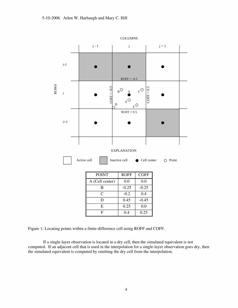
(IBOUND>0) finite-difference cell. If an observation is located at a cell center, then the simulated equivalent is equal to the model-calculated head. Observation wells, however, rarely are located at cell centers and might not be screened throughout the entire thickness represented by the model layer. To account for observation wells located horizontally away from cell centers, simulated hydraulic heads at observation locations need to be calculated by interpolating within the two-dimensional plane of a single layer. Six locations (A-F) for which hydraulic heads might need to be horizontally interpolated are shown in figure 1. Exact interpolation of hydraulic heads, in which the interpolated hydraulic heads would correspond to the hydraulic heads simulated using a locally very fine numerical grid, is not generally possible for block-centered finite-difference methods. Geometric interpolation methods that ignore the variations in hydraulic conductivity, however, are available. In this report, geometric interpolation based on linear, finite-element basis functions is used.
2
5-10-2006 Arlen W. Harbaugh and Mary C. Hill
A linear one-dimensional basis function (equivalent to linear interpolation) is used for locations that are adjacent to two inactive (no flow or constant head) cells, such as location B in figure 1. A linear basis function is also used for locations that are exactly between adjoining cell centers, such as location E. Triangular basis functions are used for locations that are within a triangle formed by the centers of three neighboring cells because the fourth neighboring cell is inactive (locations C and F in figure 1). Quadrilateral basis functions are used for locations such as D in figure 1, which are within a rectangle formed by the centers of four active cells. All basis functions are calculated using local coordinates that are specified by the user and define the observation location within a cell relative to the cell center. These local coordinates are a row offset, ROFF, and a column offset, COFF, that range in value from –0.5 to +0.5, with 0.0 indicating that there is no offset. Use of ROFF and COFF is illustrated in figure 1. Note that ROFF is negative in the direction of decreasing row numbers, and COFF is negative in the direction of decreasing column numbers.
The basis functions used are described in numerous texts and are not discussed in this report. They are equivalent to the one-dimensional simplex, two-dimensional simplex, and quadratic-element basis functions of Segerlind (1976, p. 24, 28, and 258), and the triangular "archetypal" and rectangular-element basis functions of Wang and Anderson (1982, p. 119 and 153).
Errors introduced by using geometric interpolation might become substantial when the hydraulic properties of neighboring cells are different and cell dimensions are large. At such locations, the differences between observed and simulated hydraulic heads might be inaccurate . This problem would be characterized by larger than expected differences between observed and simulated hydraulic heads.
3
5-10-2006 Arlen W. Harbaugh and Mary C. Hill
Inactive cell Cell center
COLUMNS
j
RO
WS
j - 1 j
C
OFF
= -0
.5
CO
FF =
0.5
ROFF = -0.5
ROFF = 0.5
+ 1
Point
C
FD
B
E
A
Active cell
i-1
i
i+1
EXPLANATION
POINT ROFF COFF
A (Cell center) 0.0 0.0
B -0.25 -0.25
C -0.2 0.4
D 0.45 -0.45
E 0.25 0.0
F 0.4 0.25
Figure 1: Locating points within a finite-difference cell using ROFF and COFF.
If a single-layer observation is located in a dry cell, then the simulated equivalent is not computed. If an adjacent cell that is used in the interpolation for a single-layer observation goes dry, then the simulated equivalent is computed by omitting the dry cell from the interpolation.
4
5-10-2006 Arlen W. Harbaugh and Mary C. Hill
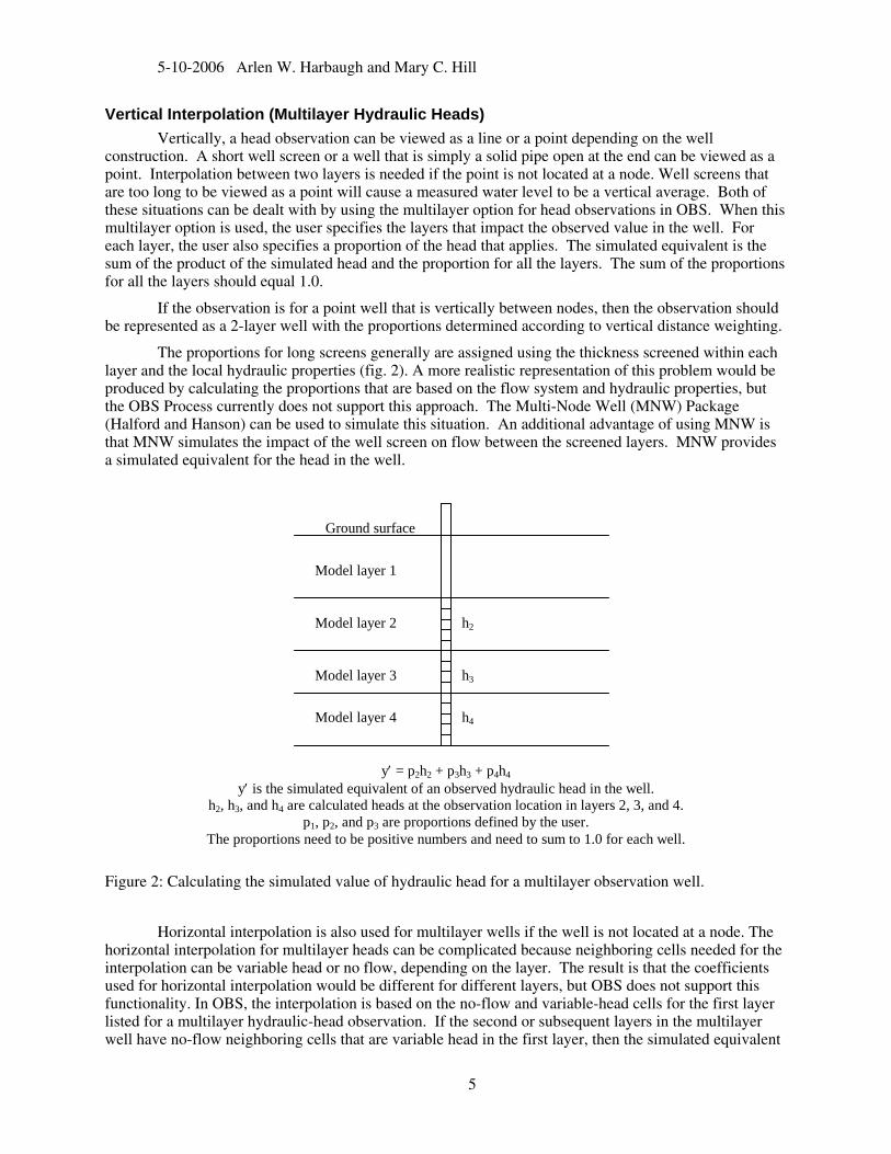
Vertical Interpolation (Multilayer Hydraulic Heads) Vertically, a head observation can be viewed as a line or a point depending on the well
construction. A short well screen or a well that is simply a solid pipe open at the end can be viewed as a point. Interpolation between two layers is needed if the point is not located at a node. Well screens that are too long to be viewed as a point will cause a measured water level to be a vertical average. Both of these situations can be dealt with by using the multilayer option for head observations in OBS. When this multilayer option is used, the user specifies the layers that impact the observed value in the well. For each layer, the user also specifies a proportion of the head that applies. The simulated equivalent is the sum of the product of the simulated head and the proportion for all the layers. The sum of the proportions for all the layers should equal 1.0.
If the observation is for a point well that is vertically between nodes, then the observation should be represented as a 2-layer well with the proportions determined according to vertical distance weighting.
The proportions for long screens generally are assigned using the thickness screened within each layer and the local hydraulic properties (fig. 2). A more realistic representation of this problem would be produced by calculating the proportions that are based on the flow system and hydraulic properties, but the OBS Process currently does not support this approach. The Multi-Node Well (MNW) Package (Halford and Hanson) can be used to simulate this situation. An additional advantage of using MNW is that MNW simulates the impact of the well screen on flow between the screened layers. MNW provides a simulated equivalent for the head in the well.
h3
h4
Model layer 1
Model layer 2
Model layer 3
Model layer 4
y′ = p2h2 + p3h3 + p4h4 y′ is the simulated equivalent of an observed hydraulic head in th
h2, h3, and h4 are calculated heads at the observation location in layersp1, p2, and p3 are proportions defined by the user.
The proportions need to be positive numbers and need to sum to 1.0 f
h2
e well. 2, 3, and 4.
or each well.
Ground surface
Figure 2: Calculating the simulated value of hydraulic head for a multilayer observation well.
Horizontal interpolation is also used for multilayer wells if the well is not located at a node. The horizontal interpolation for multilayer heads can be complicated because neighboring cells needed for the interpolation can be variable head or no flow, depending on the layer. The result is that the coefficients used for horizontal interpolation would be different for different layers, but OBS does not support this functionality. In OBS, the interpolation is based on the no-flow and variable-head cells for the first layer listed for a multilayer hydraulic-head observation. If the second or subsequent layers in the multilayer well have no-flow neighboring cells that are variable head in the first layer, then the simulated equivalent
5

5-10-2006 Arlen W. Harbaugh and Mary C. Hill
will not be computed. Two multilayer observations for which the neighboring cells have differing no-flow and variable-head status are illustrated in figure 3.
Model layer 2
Model layer 3
Model layer 4
Situation that can produce correct spatial interpolation
for multilayer hydraulic-head observations.
Model layer 4 needs to be listed
first.
Situation that can NOT produce correct spatial interpolation for
multilayer hydraulic-head observations.
No layer has no-flow cells that correspond to the no-flow cells
in all other layers.
Variable-head cell No-flow cell Cell center
(A) (B)
Obser- vation well
EXPLANATION
Figure 3: Situations for which the Observation Process (A) can and (B) cannot produce spatial
interpolation for the multilayer hydraulic-head observation shown in figure 2.
The simulated equivalent also is not computed for a multilayer observation if any cells used in the interpolation go dry. Although the cells could be omitted from the interpolation for the layers involved and a simulated head could be calculated, the proportions would no longer be valid. In addition, if the observation occurs within a time step as described in the earlier section “Observation Times”, then the simulated equivalent is not computed if any cell involved in the interpolation is dry for either time step involved.
6

5-10-2006 Arlen W. Harbaugh and Mary C. Hill
Flow Observations at Boundaries Represented as Constant Head
The Constant-Head Flow Package in OBS provides the capability to use flows to or from constant-head cells as observations. Consider a constant-head cell located at finite-difference cell n. Like all finite-difference cells in a three-dimensional grid, the constant-head cell has six faces; these faces will be numbered 1 through 6, and will be designated using p. If the cell adjacent to side p exists and is variable head (IBOUND>0), the flow through cell face p of the constant-head cell can be calculated as:
)h(H pn,np −
∑=
=6
1ppn,n qq
∑=
=′nqcl
1nnnqfy
Cq n,pn, = (1)
where
qn,p is the simulated flow rate through cell face p (L3/T) (negative for flow into the constant-head cell);
Cn,p is the conductance of the material separating the center of the constant-head finite-difference cell from the center of the cell adjacent to side p (L2/T);
hn,p is the hydraulic head in neighboring cell p (L); and
Hn is the specified hydraulic head in the constant-head cell (L).
To calculate the total flow to or from one constant-head cell, the flow through each face for which the neighboring cell exists and is not constant head needs to be accumulated. That is,
(2)
where qn is the flow into (-) or out (+) of the constant-head cell.
A constant-head flow observation commonly is represented by a group of constant-head cells. Summing over nqcl cells, the simulated equivalent to the observation (y’) equals:
(3)
where
fn is a user-defined multiplicative factor.
Generally fn = 1.0. However, fn needs to be less than 1.0 if only part of the flow calculated for the cell is to be included in the simulated equivalent to the observation.
Note that for constant-head flow observations, dry cells are not an issue because constant-head cells do not go dry.
7

5-10-2006 Arlen W. Harbaugh and Mary C. Hill
Flow Observations at Boundaries Represented as Head Dependent
Flow observations often are related to surface-water bodies such as streams and lakes. The physics of such flows often are best represented using one of the three head-dependent boundary packages of MODFLOW-2005, the General-Head Boundary, Drain, or River Package. For the three packages, figure 4 depicts how the ground-water/surface-water interaction is conceptualized, and shows all of the variables that may be included in the calculations. Not all the variables shown are used in all the packages mentioned. For all packages, the variables Kn, An, and Dn are combined to form conductance terms, and these are specified in the package input file. Details of the calculations are presented below.
An
Hn
hn
Kn, DnRBOTn
EXPLANATION
An Area of the water-body within finite difference cell n
Hn Water level in the water body within finite-difference cell n, or, for the Drain Package, the elevation of the drain
Dn Thickness of the water-body bed within finite-difference cell n
RBOTn Elevation of the bottom of the water-body bed
Kn Hydraulic conductivity of the water-body bed within finite-difference cell n
• Finite-difference cell center
hn Calculated hydraulic head for finite-difference cell n
Figure 4: Diagram depicting the quantities used to calculate flow between the ground-water system and a surface-water body.
Basic Head-Dependent Flow Calculations In many circumstances, flow between a single finite-difference cell representing the ground-water
system and the surface-water body (such as a lake or stream) is calculated as:
)h(HAK)h(HCq nnn
nn −=−=Dnnnn
(4)
where,
qn is the simulated flow rate at one cell (L3/T) (negative for flow out of the ground-water system);
Cn is the conductance of the material separating the surface-water body from the ground-water system and is defined as KnAn/Dn (L
2/T);
8
5-10-2006 Arlen W. Harbaugh and Mary C. Hill
Kn is the hydraulic conductivity (L/T) of, for example, the riverbed or lakebed;
Dn is the thickness (L) of the water-body bed within the finite-difference cell;
An is the area of the water body within the finite-difference cell (L2
);
hn is the calculated hydraulic head for finite-difference cell n (L); and
Hn is the water level in the water body within finite-difference cell n, or, for the Drain Package, the elevation of the drain (L).
A dry cell results in qn=0.0.
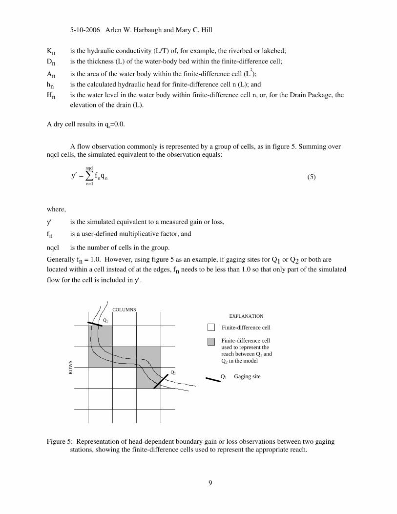
A flow observation commonly is represented by a group of cells, as in figure 5. Summing over nqcl cells, the simulated equivalent to the observation equals:
∑=
=′nqcl
1nnnqfy
(5)
where,
y′ is the simulated equivalent to a measured gain or loss,
fn is a user-defined multiplicative factor, and
nqcl is the number of cells in the group.
Generally fn = 1.0. However, using figure 5 as an example, if gaging sites for Q1 or Q2 or both are located within a cell instead of at the edges, fn needs to be less than 1.0 so that only part of the simulated
flow for the cell is included in y′.
RO
WS
Q1
Q2
COLUMNS
Finite-difference cell
Finite-difference cell used to represent the reach between Q1 and Q2 in the model
Q1 Gaging site
EXPLANATION
Figure 5: Representation of head-dependent boundary gain or loss observations between two gaging
stations, showing the finite-difference cells used to represent the appropriate reach.
9

5-10-2006 Arlen W. Harbaugh and Mary C. Hill
Modifications to the Basic Head-Dependent Flow Calculations OBS can compute flow observations for the General-head Boundary (GHB), Drain (DRN), and
River (RIV) Packages of MODFLOW (Harbaugh, 2005). The relation between calculated flow and calculated hydraulic head in the ground-water system for each package is shown in figure 6.
Positive qn indicates flow into
the subsurface
Negative qn indicates
flow out of the
subsurface Hn
qn = 0
Slope = -Cn = -(KnAn)/Dn
Positive qn indicates flow into
the subsurface
Negative qn indicates
flow out of the
subsurface RBOTn
qn = 0
Slope = -
Hn
Cn = -(KnAn)/Dn
Slope = -Cn = -(KnAn)/Dn
Hn
Negative qn indicates
flow out of the
subsurface
qn
qn
qn
hn
hn
(A)
(B)
hn
(C)
EXPLANATION
e cell (L3/T)
ound-water
/T) of, for
ed
mple, the riverbed
thin the finite-
ing Kn, Dn, and
in the ground-
ead-dependent
body or the
(L)
qn is the simulated flow rate at on
(negative for flow out of the grsystem)
Kn is the hydraulic conductivity (L
example, the riverbed or lakeb
Dn is the thickness (L) of, for exa
or lakebed
An is the area of the water body wi
difference cell (L2)
Cn is the conductance calculated usAn (L
2/T)
hn is the simulated hydraulic head
water system adjacent to the hboundary (L)
Hn is the water level in the water
elevation of the drain (L)
RBOTn is the bottom of the streambed
(C)
qn = 0
Figure 6: The dependence of simulated gains and losses on hydraulic head in the model layer (hn) in: (A)
the General-Head Boundary Package, (B) the Drain Package , and (C) the River Package.
In the General-Head Boundary Package of OBS, equation 4 is used to compute flow at each finite-difference cell, and the calculation is summed for all the cells involved (eq. 5).
In the Drain Package of OBS, flow at each specified finite-difference cell is calculated as in equation 4 except for cells in which the simulated hydraulic head (hn) falls below Hn of figure 6. For these cells the flow is set to zero, so that the Drain Package never allows flow into the ground-water system. The relation between flow and hydraulic heads is as depicted in figure 6B. Mathematically, for finite-difference cell n, this is expressed as:
10

5-10-2006 Arlen W. Harbaugh and Mary C. Hill
qn = Cn(hn - Hn)
qn = 0.0
hn>Hn
hn≤Hn
(6)
The calculation is summed for the cells involved using equation 5.
In the River Package of OBS, flow at each finite-difference cell specified is calculated using equation 4 except when the hydraulic head falls below RBOTn. The relation between flow and hydraulic head is depicted in figure 6C. Mathematically, for finite-difference cell n, this is expressed as:
qn = Cn(Hn - hn)
qn = Cn(Hn - RBOTn)
hn>RBOTn
hn<RBOTn
(7)
The calculation is summed for the cells involved using equation 5.
Observations at Cells Having More Than One Head-Dependent Boundary Feature Represented by the Same Package
MODFLOW allows occurrences of the same head-dependent boundary type in a single finite-difference cell. For example, two canals represented by the Drain Package may cross an area such that they would be represented using the same finite difference cell, as designated by its layer, row, and column. Hence, that layer, row, and column would be listed twice in the Drain Package input file.
To accumulate the information needed to define the simulated equivalent of an observation, OBS uses an observation cell list from the applicable OBS input file, which defines an observation cell group, and additional information specified in the corresponding Ground-Water Flow Process input file. The information for each cell is accumulated by matching cells listed in the Observation Process input file with those listed in the Ground-Water Flow Process input file. For the General-Head Boundary, Drain, and River Packages documented in this work, features match when the cell’s layer, row, and column match. As long as the cell occurs only once in each list of cells, no problem occurs. If the list of cells used to define the observation cell group includes a feature at a cell where more than one feature is defined for the stress period in which the observation occurs in the Ground-Water Flow input file for the same package, a procedure is needed to ensure that the correct feature is included in the simulated equivalent. In OBS, the following sequential matching procedure is used.
If a cell is listed once in the observation cell group, the simulated equivalent for the observation includes flow calculated only for the first occurrence of the cell, as listed in the Ground-Water Flow Process input file for the package of concern for the stress period in which the observation occurs. Note that the stress period in which the observation occurs may be the reference stress period for the observation, or a later stress period, depending on the length of the reference stress period and the values of the time-offset multiplier and the variable TOFFSET. The listing order of cells in the Ground-Water Flow Process input file is determined as follows: all non-parameter cells are listed before all parameter-controlled cells for a given stress period, and the order in which parameters are listed in the head-dependent boundary flow input file for each stress period determines the listing order of parameter-controlled cells. Within the list of cells controlled by a parameter, the order is determined by the cell list in the parameter definition specified near the top of the Ground-Water Flow Process input file.
When a cell in an observation cell group is to be associated with the second or later occurrence of the cell in the Ground-Water Flow Process input for a given stress period, the observation cell group needs to include two or more occurrences of the cell, where the number of occurrences corresponds to the
11

5-10-2006 Arlen W. Harbaugh and Mary C. Hill
sequential occurrence of the feature sought. Occurrences of the cell for which the flow calculated by the Ground-Water Flow Process is not to contribute to the flow observation need to be specified with FACTOR=0.0 (see preceding sections for explanation of FACTOR). For each observation cell group, the program starts at the first cell listed for the stress period in the Ground-Water Flow Process input file and searches for a match for the first cell in the observation cell group. After a match is found, appropriate calculations are done and the search for a match for the next cell in the observation cell group begins, starting at the feature following the feature matching the previous cell in the observation cell group. When the end of the list for the stress period in the Ground-Water Flow Process input file is reached, the search continues at the beginning of the list. This can be confusing and care is needed to obtain the desired results. Searching and matching continues in this fashion until all cells in the observation cell group are matched. For the next observation cell group, the search starts at the beginning of the list for the stress period in the Ground-Water Flow Process input file.
Understanding this search logic is necessary when determining the order in which cells are listed in an observation cell group to ensure that observation cells are matched as intended with features listed for the Ground-Water Flow Process. When the features simulated by a particular package change from one stress period to the next, the list of cells in an observation cell group may not apply appropriately to both stress periods. In this situation, multiple cell groups may need to be defined to specify flow observations in different stress periods.
As an example, consider a model for an area where a series of springs discharge water from intervals at different elevations in an aquifer. For this model, the Drain Package is used and three drain features are specified in each of three finite-difference cells, for a total of nine features. All features are defined using parameters. One parameter is used to simulate three drain features, in rows 5, 6, and 7 of column 6; the elevations of these drain features are 20, 22, and 24 in this model. A second parameter is used to simulate drain features in the same three cells, each having an elevation of 30. A third parameter is used to simulate drain features in the same three cells; the elevation is 45 at the first two cells, and 47 at the third cell. For this model, the Ground-Water Flow Process Drain Package input file, listed with file type DRN in the name file, is as follows:
# DRN input file parameter 3 9 Item 1: npdrn mxl 10 0 Item 2: mxactd idrncb drn-low drn 10.0 3 Item 3: parnam partyp parval nlst 1 5 6 20 1.0 Item 4: lay row col elev condfact 1 6 6 22 1.0 Item 4: lay row col elev condfact 1 7 6 24 1.0 Item 4: lay row col elev condfact drn-med drn 1.0 3 Item 3: parnam partyp parval nlst 1 5 6 30 1.0 Item 4: lay row col elev condfact 1 6 6 30 1.0 Item 4: lay row col elev condfact 1 7 6 30 1.0 Item 4: lay row col elev condfact drn-high drn 10.0 3 Item 3: parnam partyp parval nlst 1 5 6 45 1.0 Item 4: lay row col elev condfact 1 6 6 45 1.0 Item 4: lay row col elev condfact 1 7 6 47 1.0 Item 4: lay row col elev condfact 0 3 Item 5: itmp np drn-low Item 7: Pname drn-med Item 7: Pname drn-high Item 7: Pname
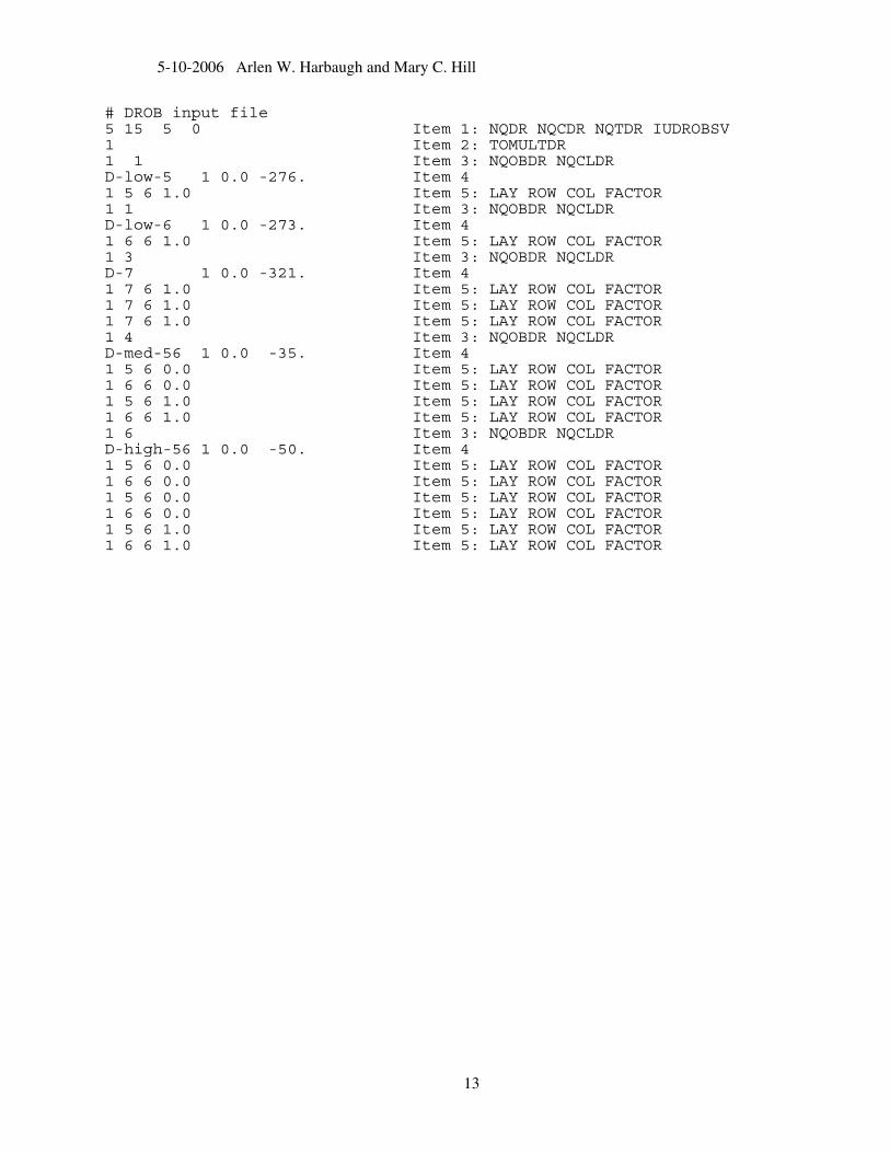
Observations of flow from the springs are represented such that the drain features in rows 5 and 6 at elevations 20 and 22 are associated with observations named D-low-5 and D-low-6, respectively; all the drain features in row 7 are together associated with an observation named D-7, the drain features in rows 5 and 6 at elevation 30 are together associated with an observation named D-med-56, and the springs in rows 5 and 6 at elevation 45 are associated with an observation named D-high-56. The following DROB file correctly associates the five observations with the nine drain features:
12
5-10-2006 Arlen W. Harbaugh and Mary C. Hill
# DROB input file 5 15 5 0 Item 1: NQDR NQCDR NQTDR IUDROBSV 1 Item 2: TOMULTDR 1 1 Item 3: NQOBDR NQCLDR D-low-5 1 0.0 -276. Item 4 1 5 6 1.0 Item 5: LAY ROW COL FACTOR 1 1 Item 3: NQOBDR NQCLDR D-low-6 1 0.0 -273. Item 4 1 6 6 1.0 Item 5: LAY ROW COL FACTOR 1 3 Item 3: NQOBDR NQCLDR D-7 1 0.0 -321. Item 4 1 7 6 1.0 Item 5: LAY ROW COL FACTOR 1 7 6 1.0 Item 5: LAY ROW COL FACTOR 1 7 6 1.0 Item 5: LAY ROW COL FACTOR 1 4 Item 3: NQOBDR NQCLDR D-med-56 1 0.0 -35. Item 4 1 5 6 0.0 Item 5: LAY ROW COL FACTOR 1 6 6 0.0 Item 5: LAY ROW COL FACTOR 1 5 6 1.0 Item 5: LAY ROW COL FACTOR 1 6 6 1.0 Item 5: LAY ROW COL FACTOR 1 6 Item 3: NQOBDR NQCLDR D-high-56 1 0.0 -50. Item 4 1 5 6 0.0 Item 5: LAY ROW COL FACTOR 1 6 6 0.0 Item 5: LAY ROW COL FACTOR 1 5 6 0.0 Item 5: LAY ROW COL FACTOR 1 6 6 0.0 Item 5: LAY ROW COL FACTOR 1 5 6 1.0 Item 5: LAY ROW COL FACTOR 1 6 6 1.0 Item 5: LAY ROW COL FACTOR
13
5-10-2006 Arlen W. Harbaugh and Mary C. Hill
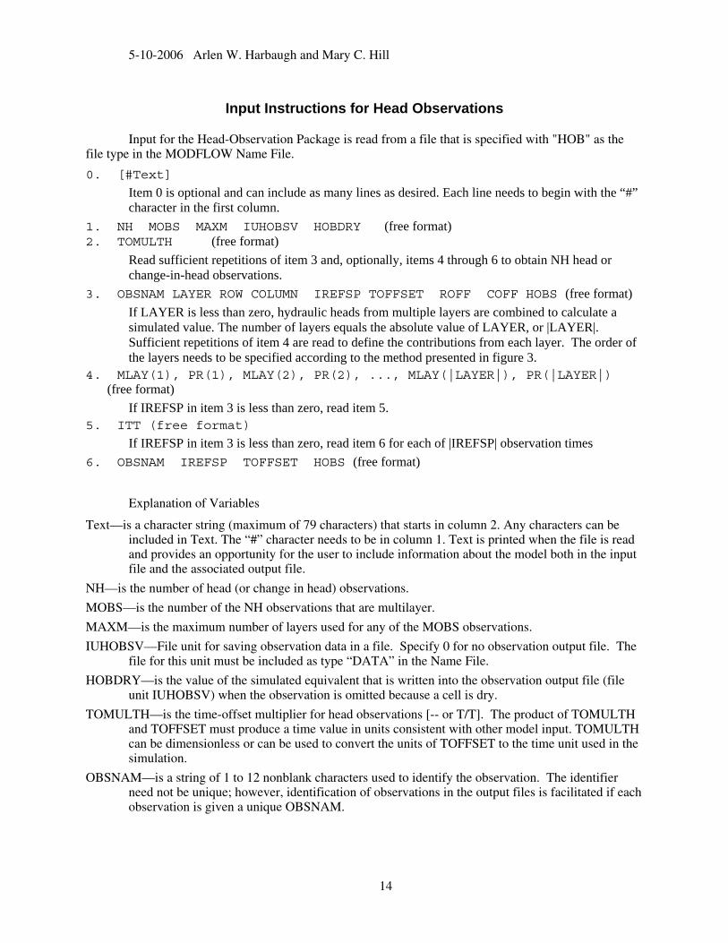
Input Instructions for Head Observations
Input for the Head-Observation Package is read from a file that is specified with "HOB" as the file type in the MODFLOW Name File.
0. [#Text]
Item 0 is optional and can include as many lines as desired. Each line needs to begin with the “#” character in the first column.
1. NH MOBS MAXM IUHOBSV HOBDRY (free format) 2. TOMULTH (free format)
Read sufficient repetitions of item 3 and, optionally, items 4 through 6 to obtain NH head or change-in-head observations.
3. OBSNAM LAYER ROW COLUMN IREFSP TOFFSET ROFF COFF HOBS (free format) If LAYER is less than zero, hydraulic heads from multiple layers are combined to calculate a simulated value. The number of layers equals the absolute value of LAYER, or |LAYER|. Sufficient repetitions of item 4 are read to define the contributions from each layer. The order of the layers needs to be specified according to the method presented in figure 3.
4. MLAY(1), PR(1), MLAY(2), PR(2), ..., MLAY(|LAYER|), PR(|LAYER|) (free format)
If IREFSP in item 3 is less than zero, read item 5. 5. ITT (free format)
If IREFSP in item 3 is less than zero, read item 6 for each of |IREFSP| observation times 6. OBSNAM IREFSP TOFFSET HOBS (free format)
Explanation of Variables
Text—is a character string (maximum of 79 characters) that starts in column 2. Any characters can be included in Text. The “#” character needs to be in column 1. Text is printed when the file is read and provides an opportunity for the user to include information about the model both in the input file and the associated output file.
NH—is the number of head (or change in head) observations.
MOBS—is the number of the NH observations that are multilayer.
MAXM—is the maximum number of layers used for any of the MOBS observations.
IUHOBSV—File unit for saving observation data in a file. Specify 0 for no observation output file. The file for this unit must be included as type “DATA” in the Name File.
HOBDRY—is the value of the simulated equivalent that is written into the observation output file (file unit IUHOBSV) when the observation is omitted because a cell is dry.
TOMULTH—is the time-offset multiplier for head observations [-- or T/T]. The product of TOMULTH and TOFFSET must produce a time value in units consistent with other model input. TOMULTH can be dimensionless or can be used to convert the units of TOFFSET to the time unit used in the simulation.
OBSNAM—is a string of 1 to 12 nonblank characters used to identify the observation. The identifier need not be unique; however, identification of observations in the output files is facilitated if each observation is given a unique OBSNAM.
14
5-10-2006 Arlen W. Harbaugh and Mary C. Hill
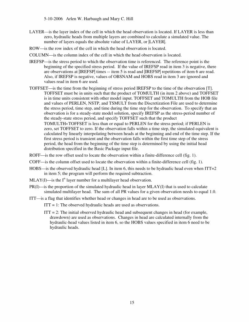
LAYER—is the layer index of the cell in which the head observation is located. If LAYER is less than zero, hydraulic heads from multiple layers are combined to calculate a simulated value. The number of layers equals the absolute value of LAYER, or |LAYER|.
ROW—is the row index of the cell in which the head observation is located.
COLUMN—is the column index of the cell in which the head observation is located.
IREFSP—is the stress period to which the observation time is referenced. The reference point is the beginning of the specified stress period. If the value of IREFSP read in item 3 is negative, there are observations at |IREFSP| times -- item 5 is read and |IREFSP| repetitions of item 6 are read. Also, if IREFSP is negative, values of OBSNAM and HOBS read in item 3 are ignored and values read in item 6 are used.
TOFFSET—is the time from the beginning of stress period IREFSP to the time of the observation [T]. TOFFSET must be in units such that the product of TOMULTH (in item 2 above) and TOFFSET is in time units consistent with other model input. TOFFSET and TOMULTH from the HOB file and values of PERLEN, NSTP, and TSMULT from the Discretization File are used to determine the stress period, time step, and time during the time step for the observation. To specify that an observation is for a steady-state model solution, specify IREFSP as the stress-period number of the steady-state stress period, and specify TOFFSET such that the product TOMULTH×TOFFSET is less than or equal to PERLEN for the stress period; if PERLEN is zero, set TOFFSET to zero. If the observation falls within a time step, the simulated equivalent is calculated by linearly interpolating between heads at the beginning and end of the time step. If the first stress period is transient and the observation falls within the first time step of the stress period, the head from the beginning of the time step is determined by using the initial head distribution specified in the Basic Package input file.
ROFF—is the row offset used to locate the observation within a finite-difference cell (fig. 1).
COFF—is the column offset used to locate the observation within a finite-difference cell (fig. 1).
HOBS—is the observed hydraulic head [L]. In item 6, this needs to be hydraulic head even when ITT=2 in item 5; the program will perform the required subtraction.
MLAY(I)—is the Ith layer number for a multilayer head observation.
PR(I)—is the proportion of the simulated hydraulic head in layer MLAY(I) that is used to calculate simulated multilayer head. The sum of all PR values for a given observation needs to equal 1.0.
ITT—is a flag that identifies whether head or changes in head are to be used as observations.
ITT = 1: The observed hydraulic heads are used as observations.
ITT = 2: The initial observed hydraulic head and subsequent changes in head (for example, drawdown) are used as observations. Changes in head are calculated internally from the hydraulic-head values listed in item 6, so the HOBS values specified in item 6 need to be hydraulic heads.
15
5-10-2006 Arlen W. Harbaugh and Mary C. Hill
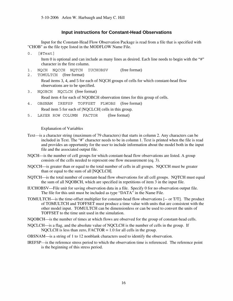
Input instructions for Constant-Head Observations
Input for the Constant-Head Flow Observation Package is read from a file that is specified with "CHOB" as the file type listed in the MODFLOW Name File.
0. [#Text]
Item 0 is optional and can include as many lines as desired. Each line needs to begin with the “#” character in the first column.
1. NQCH NQCCH NQTCH IUCHOBSV (free format) 2. TOMULTCH (free format)
Read items 3, 4, and 5 for each of NQCH groups of cells for which constant-head flow observations are to be specified.
3. NQOBCH NQCLCH (free format) Read item 4 for each of NQOBCH observation times for this group of cells.
4. OBSNAM IREFSP TOFFSET FLWOBS (free format) Read item 5 for each of |NQCLCH| cells in this group.
5. LAYER ROW COLUMN FACTOR (free format)
Explanation of Variables
Text—is a character string (maximum of 79 characters) that starts in column 2. Any characters can be included in Text. The “#” character needs to be in column 1. Text is printed when the file is read and provides an opportunity for the user to include information about the model both in the input file and the associated output file.
NQCH—is the number of cell groups for which constant-head flow observations are listed. A group consists of the cells needed to represent one flow measurement (eq. 3).
NQCCH—is greater than or equal to the total number of cells in all groups. NQCCH must be greater than or equal to the sum of all |NQCLCH|.
NQTCH—is the total number of constant-head flow observations for all cell groups. NQTCH must equal the sum of all NQOBCH, which are specified in repetitions of item 3 in the input file.
IUCHOBSV—File unit for saving observation data in a file. Specify 0 for no observation output file. The file for this unit must be included as type “DATA” in the Name File.
TOMULTCH—is the time-offset multiplier for constant-head flow observations [-- or T/T]. The product of TOMULTCH and TOFFSET must produce a time value with units that are consistent with the other model input. TOMULTCH can be dimensionless or can be used to convert the units of TOFFSET to the time unit used in the simulation.
NQOBCH—is the number of times at which flows are observed for the group of constant-head cells.
NQCLCH—is a flag, and the absolute value of NQCLCH is the number of cells in the group. If NQCLCH is less than zero, FACTOR = 1.0 for all cells in the group.
OBSNAM—is a string of 1 to 12 nonblank characters used to identify the observation.
IREFSP—is the reference stress period to which the observation time is referenced. The reference point is the beginning of this stress period.
16

5-10-2006 Arlen W. Harbaugh and Mary C. Hill
TOFFSET—is the time offset of the observation, from the beginning of stress period IREFSP [T]. TOFFSET must be in units such that the product of TOMULTCH and TOFFSET is in time units consistent with other model input. TOFFSET and TOMULTCH from the CHOB file and values of PERLEN, NSTP, and TSMULT from the Discretization File (Harbaugh, 2005) are used to determine the stress period, time step, and time during the time step for the observation. To specify that an observation is for a steady-state model solution, specify IREFSP as the stress-period number of the steady-state stress period, and specify TOFFSET such that the product TOMULTCH × TOFFSET is less than or equal to PERLEN for the stress period; if PERLEN is zero, set TOFFSET to zero. If the observation falls within a time step, the simulated equivalent is calculated by linearly interpolating between values for the beginning and end of the time step. If the first stress period is transient and the observation falls within the first time step, the simulated equivalent from the end of the time step is used because no flow from the beginning of the time step is available for interpolation.
FLWOBS—is the observed flow from the constant-head boundary into the aquifer (positive) or the flow from the aquifer into the constant-head boundary (negative) [L3/T].
LAYER—is the layer index of a constant-head cell included in the cell group.
ROW—is the row index of a constant-head cell included in the cell group.
COLUMN—is the column index of a constant-head cell included in the cell group.
FACTOR—is the portion of the simulated flow for the cell that is included in the total simulated flow for this cell group (fn of eq. 3).
17

5-10-2006 Arlen W. Harbaugh and Mary C. Hill
Input Instructions for General-Head Boundary Observations
Input for the General-Head-Boundary Observation Package is read from a file that is specified with "GBOB" as the file type listed in the MODFLOW Name File.
0. [#Text]
Item 0 is optional and can include as many lines as desired. Each line needs to begin with the “#” character in the first column.
1. NQGB NQCGB NQTGB IUGBOBSV (free format) 2. TOMULTGB (free format)
Read items 3, 4, and 5 for each of NQGB groups of cells for which general-head-boundary observations are to be specified.
3. NQOBGB NQCLGB (free format) Read item 4 for each of NQOBGB observation times for this group of cells.
4. OBSNAM IREFSP TOFFSET FLWOBS (free format) Read item 5 for each of |NQCLGB| cells in this group.
5. LAYER ROW COLUMN FACTOR (free format) Read items 6 and 7 if IOWTQGB is greater than 0.
Explanation of Variables
Text—is a character string (maximum of 79 characters) that starts in column 2. Any characters can be included in Text. The “#” character needs to be in column 1. Text is printed when the file is read and provides an opportunity for the user to include information about the model both in the input file and the associated output file.
NQGB—is the number of cell groups for which general-head-boundary observations are listed. A group consists of the cells needed to represent one flow measurement (eq. 5).
NQCGB—is greater than or equal to the total number of cells in all cell groups. NQCGB must be greater than or equal to the sum of all |NQCLGB|.
NQTGB—is the total number of general-head-boundary observations for all cell groups. NQTGB must equal the sum of all NQOBGB, which are specified in repetitions of item 3 in the input file.
IUGBOBSV—File unit for saving observation data in a file. Specify 0 for no observation output file. The file for this unit must be included as type “DATA” in the Name File.
TOMULTGB—is the time-offset multiplier for general-head-boundary observations [-- or T/T]. The product of TOMULTGB and TOFFSET must produce a time value in units consistent with other model input. TOMULTGB can be dimensionless or can be used to convert the units of TOFFSET to the time unit used in the simulation.
NQOBGB—is the number of times at which flows are observed for the group of cells.
NQCLGB—is a flag, and the absolute value of NQCLGB is the number of cells in the group. If NQCLGB is less than zero, FACTOR = 1.0 for all cells in the group.
OBSNAM—is a string of 1 to 12 nonblank characters used to identify the observation.
IREFSP—is the reference stress period to which the observation time is referenced. The reference point is the beginning of the stress period.
18

5-10-2006 Arlen W. Harbaugh and Mary C. Hill
TOFFSET—is the time from the beginning of stress period IREFSP to the time of the observation [T]. TOFFSET must be in units such that the product of TOMULTGB and TOFFSET is in time units consistent with other model input. TOFFSET and TOMULTGB from the GBOB file and values of PERLEN, NSTP, and TSMULT from the Discretization File (Harbaugh, 2005) are used to determine the stress period, time step, and time during the time step for the observation. To specify that an observation is for a steady-state model solution, specify IREFSP as the stress-period number of the steady-state stress period, and specify TOFFSET such that the product TOMULTGB×TOFFSET is less than or equal to PERLEN for the stress period; if PERLEN is zero, set TOFFSET to zero. If the observation falls within a time step, the simulated equivalent is calculated by linearly interpolating between values for the beginning and end of the time step. If the first stress period is transient and the observation falls within the first time step, the simulated equivalent from the end of the time step is used because no flow from the beginning of the time step is available for interpolation.
FLWOBS—is the observed flow from the general-head boundary into the aquifer (positive) or the flow from the aquifer into the boundary (negative) [L3/T].
LAYER—is the layer index of a general-head-boundary cell included in the cell group.
ROW—is the row index of a general-head-boundary cell included in the cell group.
COLUMN—is the column index of a general-head-boundary cell included in the cell group.
FACTOR—is the portion of the simulated gain or loss in the cell that is included in the total simulated gain or loss for this cell group (fn of eq. 5).
19
5-10-2006 Arlen W. Harbaugh and Mary C. Hill
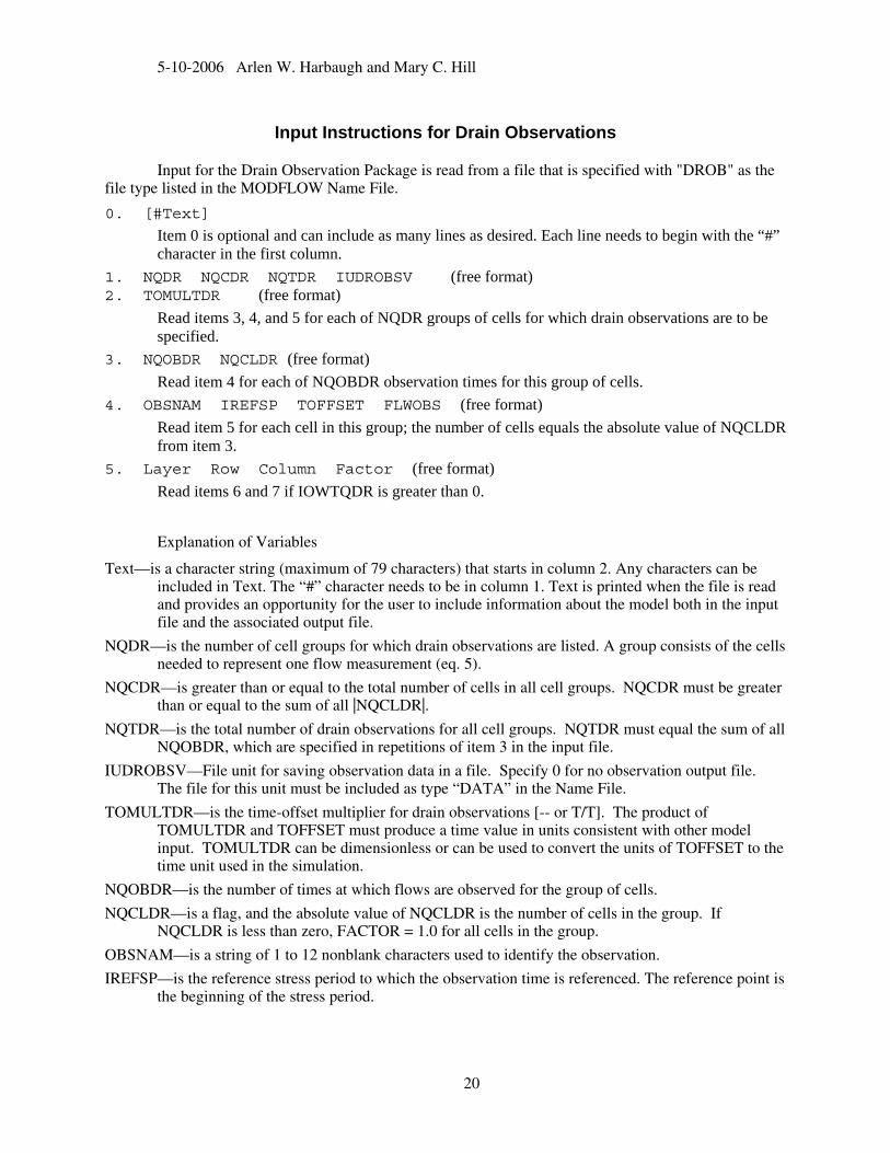
Input Instructions for Drain Observations
Input for the Drain Observation Package is read from a file that is specified with "DROB" as the file type listed in the MODFLOW Name File.
0. [#Text]
Item 0 is optional and can include as many lines as desired. Each line needs to begin with the “#” character in the first column.
1. NQDR NQCDR NQTDR IUDROBSV (free format) 2. TOMULTDR (free format)
Read items 3, 4, and 5 for each of NQDR groups of cells for which drain observations are to be specified.
3. NQOBDR NQCLDR (free format) Read item 4 for each of NQOBDR observation times for this group of cells.
4. OBSNAM IREFSP TOFFSET FLWOBS (free format) Read item 5 for each cell in this group; the number of cells equals the absolute value of NQCLDR from item 3.
5. Layer Row Column Factor (free format) Read items 6 and 7 if IOWTQDR is greater than 0.
Explanation of Variables
Text—is a character string (maximum of 79 characters) that starts in column 2. Any characters can be included in Text. The “#” character needs to be in column 1. Text is printed when the file is read and provides an opportunity for the user to include information about the model both in the input file and the associated output file.
NQDR—is the number of cell groups for which drain observations are listed. A group consists of the cells needed to represent one flow measurement (eq. 5).
NQCDR—is greater than or equal to the total number of cells in all cell groups. NQCDR must be greater than or equal to the sum of all |NQCLDR|.
NQTDR—is the total number of drain observations for all cell groups. NQTDR must equal the sum of all NQOBDR, which are specified in repetitions of item 3 in the input file.
IUDROBSV—File unit for saving observation data in a file. Specify 0 for no observation output file. The file for this unit must be included as type “DATA” in the Name File.
TOMULTDR—is the time-offset multiplier for drain observations [-- or T/T]. The product of TOMULTDR and TOFFSET must produce a time value in units consistent with other model input. TOMULTDR can be dimensionless or can be used to convert the units of TOFFSET to the time unit used in the simulation.
NQOBDR—is the number of times at which flows are observed for the group of cells.
NQCLDR—is a flag, and the absolute value of NQCLDR is the number of cells in the group. If NQCLDR is less than zero, FACTOR = 1.0 for all cells in the group.
OBSNAM—is a string of 1 to 12 nonblank characters used to identify the observation.
IREFSP—is the reference stress period to which the observation time is referenced. The reference point is the beginning of the stress period.
20

5-10-2006 Arlen W. Harbaugh and Mary C. Hill
TOFFSET—is the time from the beginning of stress period IREFSP to the time of the observation [T]. TOFFSET must be in units such that the product of TOMULTDR and TOFFSET is in time units consistent with other model input. TOFFSET and TOMULTDR from the DROB file and values of PERLEN, NSTP, and TSMULT from the Discretization File (Harbaugh, 2005) are used to determine the stress period, time step, and time during the time step for the observation. To specify that an observation is for a steady-state model solution, specify IREFSP as the stress-period number of the steady-state stress period, and specify TOFFSET such that TOMULTDR×TOFFSET is less than or equal to PERLEN for the stress period; if PERLEN is zero, set TOFFSET to zero. If the observation falls within a time step, the simulated equivalent is calculated by linearly interpolating between values for the beginning and end of the time step. If the first stress period is transient and the observation falls within the first time step, the simulated equivalent from the end of the time step is used because no flow from the beginning of the time step is available for interpolation.
FLWOBS—is the observed drain-boundary flow [L3/T]. For the Drain Package only negative values of FLWOBS are expected. Negative values indicate flow out of the ground-water system.
LAYER—is the layer index of a drain cell included in the cell group.
ROW—is the row index of a drain cell included in the cell group.
COLUMN—is the column index of a drain cell included in the cell group.
FACTOR—is the portion of the simulated drain flow in the cell that is included in the total simulated drain flow for this cell group (fn of eq. 5).
21

5-10-2006 Arlen W. Harbaugh and Mary C. Hill
Input Instructions for River Observations
Input for the River Observation Package is read from a file that is specified with "RVOB" as the file type in the MODFLOW Name File.
0. [#Text]
Item 0 is optional and can include as many lines as desired. Each line needs to begin with the “#” character in the first column.
1. NQRV NQCRV NQTRV IURVOBSV (free format) 2. TOMULTRV (free format)
Read items 3, 4, and 5 for each of NQRV groups of cells for which river observations are to be specified.
3. NQOBRV NQCLRV (free format) Read item 4 for each of NQOBRV observation times for this group of cells.
4. OBSNAM IREFSP TOFFSET FLWOBS (free format) Read item 5 for each cell in this group; the number of cells is equal to the absolute value of NQCLRV read in item 3.
5. LAYER ROW COLUMN FACTOR (free format) Read items 6 and 7 if IOWTQRV is greater than 0.
Explanation of Variables
Text—is a character string (maximum of 79 characters) that starts in column 2. Any characters can be included in Text. The “#” character needs to be in column 1. Text is printed when the file is read and provides an opportunity for the user to include information about the model both in the input file and the associated output file.
NQRV—is the number of cell groups for which river observations are listed. A group consists of the cells needed to represent one flow measurement (eq. 5).
NQCRV—is greater than or equal to the total number of cells in all cell groups. NQCRV must be greater than or equal to the sum of all of the cells listed in all cell groups; that is, NQCRV needs to exceed the sum of the absolute values of all of the NQCLRV variables in the repetitions of item 3.
NQTRV—is the total number of river observations for all cell groups. NQTRV must equal the sum of all NQOBRV, which are specified in repetitions of item 3 in the input file.
IURVOBSV—File unit for saving observation data in a file. Specify 0 for no observation output file. The file for this unit must be included as type “DATA” in the Name File.
TOMULTRV—is the time-offset multiplier for river observations [-- or T/T]. The product of TOMULTRV and TOFFSET must produce a time value in units consistent with other model input. TOMULTRV can be dimensionless or can be used to convert the units of TOFFSET to the time unit used in the simulation.
NQOBRV—is the number of times at which flows are observed for the group of cells.
NQCLRV—is a flag, and the absolute value of NQCLRV is the number of cells in the group. If NQCLRV is less than zero, FACTOR = 1.0 for all cells in the group.
OBSNAM—is a string of 1 to 12 nonblank characters used to identify the observation.
22
5-10-2006 Arlen W. Harbaugh and Mary C. Hill
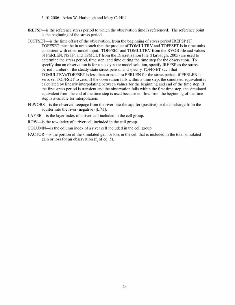
IREFSP—is the reference stress period to which the observation time is referenced. The reference point is the beginning of the stress period.
TOFFSET—is the time offset of the observation, from the beginning of stress period IREFSP [T]. TOFFSET must be in units such that the product of TOMULTRV and TOFFSET is in time units consistent with other model input. TOFFSET and TOMULTRV from the RVOB file and values of PERLEN, NSTP, and TSMULT from the Discretization File (Harbaugh, 2005) are used to determine the stress period, time step, and time during the time step for the observation. To specify that an observation is for a steady-state model solution, specify IREFSP as the stress-period number of the steady-state stress period, and specify TOFFSET such that TOMULTRV×TOFFSET is less than or equal to PERLEN for the stress period; if PERLEN is zero, set TOFFSET to zero. If the observation falls within a time step, the simulated equivalent is calculated by linearly interpolating between values for the beginning and end of the time step. If the first stress period is transient and the observation falls within the first time step, the simulated equivalent from the end of the time step is used because no flow from the beginning of the time step is available for interpolation.
FLWOBS—is the observed seepage from the river into the aquifer (positive) or the discharge from the aquifer into the river (negative) [L3/T].
LAYER—is the layer index of a river cell included in the cell group.
ROW—is the row index of a river cell included in the cell group.
COLUMN—is the column index of a river cell included in the cell group.
FACTOR—is the portion of the simulated gain or loss in the cell that is included in the total simulated gain or loss for an observation (fn of eq. 5).
23
5-10-2006 Arlen W. Harbaugh and Mary C. Hill
Code Modification
This section describes the code changes to the Observation Process from MODFLOW-2000 (Hill and others, 2000) for use in MODFLOW-2005 (Harbaugh, 2005). This version of OBS is designated OBS2. OBS2 consists of 5 packages – Basic (BAS), Constant Head (CHD), General-Head Boundary (GHB), River (RIV), and Drain (DRN). All parts that compute observation weights and weighted sum of squared residuals were removed, and the code was reorganized slightly; however, the code used to compute simulated equivalents has not been changed. Sum of squared difference between the simulated and observed values is computed for each observation type.
Each package has four primary subroutines: Allocate and Read (AR), Simulated Equivalent (SE), Output (OT), and Deallocate (DA). All subroutines designate 7 for the package version, for example OBS2BAS7AR. The AR subroutines use ALLOCATE statements to reserve memory for the data in their respective modules rather than reserving space in the X, Z, and IX arrays used by MODFLOW-2000.
To support the Local Grid Refinement capability, subroutines were created to set pointers to a grid (SOBS2BAS7PNT, for example), and subroutines were created to save the pointers for a grid (SOBS2BAS7PSV, for example). The grid number, IGRID, was added as a subroutine argument to the OBS2 subroutines as appropriate.
OBS2BAS7 computes ITS, the sequential time step counter. OBS uses ITS for tracking when observations occur rather than using stress period and time step numbers. Thus, even if there are no head observations, OBS2BAS7AR and OBS2BAS7SE must be called from the MAIN Program to compute ITS.
OBS2 stores data differently than OBS1. OBS1 establishes global observation variables for storing observation data of all types; conversely, each OBS2 package maintains the data for a particular kind of observation using variables that are internal to that package. It is still possible, however, to obtain a single output file of all observations by specifying the same file unit for saving data for all the observation packages.
Fortran modules were created to store the shared data for each package: OBSBASMODULE, OBSCHDMODULE, OBSGHBMODULE, OBSRIVMODULE, and OBSDRNMODULE. Data that are contained in Fortran modules are passed to subroutines using USE statements. See Chapter 9 of Harbaugh (2005) for further information about the use of Fortran modules in MODFLOW-2005. The following tables describe the data stored in OBS modules.
24
5-10-2006 Arlen W. Harbaugh and Mary C. Hill
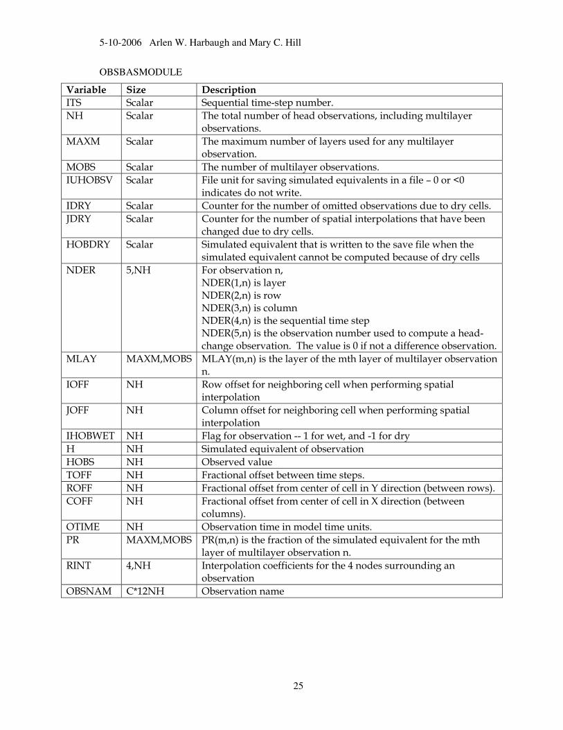
OBSBASMODULE
Variable Size Description ITS Scalar Sequential time-step number. NH Scalar The total number of head observations, including multilayer
observations. MAXM Scalar The maximum number of layers used for any multilayer
observation. MOBS Scalar The number of multilayer observations. IUHOBSV Scalar File unit for saving simulated equivalents in a file – 0 or <0
indicates do not write. IDRY Scalar Counter for the number of omitted observations due to dry cells. JDRY Scalar Counter for the number of spatial interpolations that have been
changed due to dry cells. HOBDRY Scalar Simulated equivalent that is written to the save file when the
simulated equivalent cannot be computed because of dry cells NDER 5,NH For observation n,
NDER(1,n) is layer NDER(2,n) is row NDER(3,n) is column NDER(4,n) is the sequential time step NDER(5,n) is the observation number used to compute a head-change observation. The value is 0 if not a difference observation.
MLAY MAXM,MOBS MLAY(m,n) is the layer of the mth layer of multilayer observation n.
IOFF NH Row offset for neighboring cell when performing spatial interpolation
JOFF NH Column offset for neighboring cell when performing spatial interpolation
IHOBWET NH Flag for observation -- 1 for wet, and -1 for dry H NH Simulated equivalent of observation HOBS NH Observed value TOFF NH Fractional offset between time steps. ROFF NH Fractional offset from center of cell in Y direction (between rows). COFF NH Fractional offset from center of cell in X direction (between
columns). OTIME NH Observation time in model time units. PR MAXM,MOBS PR(m,n) is the fraction of the simulated equivalent for the mth
layer of multilayer observation n. RINT 4,NH Interpolation coefficients for the 4 nodes surrounding an
observation OBSNAM C*12NH Observation name
25

5-10-2006 Arlen W. Harbaugh and Mary C. Hill
OBSCHDMODULE
Variable Size Description NQCH Scalar The number of cell groups. NQCCH Scalar The total number of cells in all cell groups. NQTCH Scalar The number of flow observations, which is the sum of the
number of observation times for all cell groups – 0 or <0 indicates do not write.
IUCHOBSV Scalar File unit for saving simulated equivalents in a file. NQOBCH NQCH The number of observation times for a cell group NQCLCH NQCH The number of cells in a cell group. IOBTS NQTCH The sequential time step number for an observation. FLWSIM NQTCH Simulated equivalent of flow. FLWOBS NQTCH Observed flow. TOFF NQTCH Fractional offset between time steps. OTIME NQTCH Observation time in model time units. QCELL 4,NQCCH Layer, row, column, and FACTOR for cells included in
observations. FACTOR is a value from 0 to 1 that is multiplied by the computed seepage at a cell to determine the contribution to the simulated equivalent seepage for the cell.
OBSNAM C*12,NQTCH Observation name.
OBSGHBMODULE
Variable Size Description NQGB Scalar The number of cell groups. NQCGB Scalar The total number of cells in all cell groups. NQTGB Scalar The number of flow observations, which is the sum of the number
of observation times for all cell groups. IUGBOBSV Scalar File unit for saving simulated equivalents in a file – 0 or <0
indicates do not write. NQOBGB NQCB The number of observation times for a cell group NQCLGB NQGB The number of cells in a cell group. IOBTS NQTGB The sequential time step number for an observation. FLWSIM NQTGB Simulated equivalent of flow. FLWOBS NQTGB Observed flow. TOFF NQTGB Fractional offset between time steps. OTIME NQTGB Observation time in model time units. QCELL 4,NQCGB Layer, row, column, and FACTOR for cells included in
observations. FACTOR is a value from 0 to 1 that is multiplied by the computed seepage at a cell to determine the contribution to the simulated equivalent seepage for the cell.
OBSNAM C*12,NQTGB Observation name.
26

5-10-2006 Arlen W. Harbaugh and Mary C. Hill
OBSDRNMODULE
Variable Size Description NQDR Scalar The number of cell groups. NQCDR Scalar The total number of cells in all cell groups. NQTDR Scalar The number of flow observations, which is the sum of the number
of observation times for all cell groups. IUDROBSV Scalar File unit for saving simulated equivalents in a file – 0 or <0
indicates do not write. NQOBDR NQDR The number of observation times for a cell group NQCLDR NQDR The number of cells in a cell group. IOBTS NQTDR The sequential time step number for an observation. FLWSIM NQTDR Simulated equivalent of flow. FLWOBS NQTDR Observed flow. TOFF NQTDR Fractional offset between time steps. OTIME NQTDR Observation time in model time units. QCELL 4,NQCDR Layer, row, column, and FACTOR for cells included in
observations. FACTOR is a value from 0 to 1 that is multiplied by the computed seepage at a cell to determine the contribution to the simulated equivalent seepage for the cell.
OBSNAM C*12,NQTDR Observation name.
OBSRIVMODULE
Variable Size Description NQRV Scalar The number of cell groups. NQCRV Scalar The total number of cells in all cell groups. NQTRV Scalar The number of flow observations, which is the sum of the number
of observation times for all cell groups. IURVOBSV Scalar File unit for saving simulated equivalents in a file – 0 or <0
indicates do not write. NQOBRV NQRV The number of observation times for a cell group NQCLRV NQRV The number of cells in a cell group. IOBTS NQTRV The sequential time step number for an observation. FLWSIM NQTRV Simulated equivalent of flow. FLWOBS NQTRV Observed flow. TOFF NQTRV Fractional offset between time steps. OTIME NQTRV Observation time in model time units. QCELL 4,NQCRV Layer, row, column, and FACTOR for cells included in
observations. FACTOR is a value from 0 to 1 that is multiplied by the computed seepage at a cell to determine the contribution to the simulated equivalent seepage for the cell.
OBSNAM C*12,NQTRV Observation name.
27
5-10-2006 Arlen W. Harbaugh and Mary C. Hill
REFERENCES
Halford, K.J. and Hanson, R.T., 2002, User guide for the Drawdown-Limited, Multi-Node Well (MNW) Package for the U.S. Geological Survey’s modular three-dimensional finite-difference ground-water flow model, versions MODFLOW-96 and MODFLOW-2000: U.S. Geological Survey Open-File Report 02-293, 33 p.
Harbaugh, A.W., 2005, MODFLOW-2005, the U.S. Geological Survey Modular Ground-Water Model—the Ground-Water Flow Process: U.S. Geological Survey Techniques and Methods 6-A16, variously p.
Harbaugh, A.W., Banta, E.R., Hill, M.C., and McDonald, M.G., 2000, MODFLOW-2000, the U.S. Geological Survey modular ground-water model – user guide to modularization concepts and the ground-water flow process: U.S. Geological Survey Open-File Report 00-92, 121 p.
Hill, M.C., Banta, E.R., Harbaugh, A.W., and Anderman, E.R., 2000, MODFLOW-2000, the U.S. Geological Survey modular ground-water model – user guide to the Observation, Sensitivity, and Parameter-Estimation Processes and three post-processing programs: U.S. Geological Survey Open-File Report 00-184, 209 p.
Poeter, E.P, Hill, M.C., Banta, E.R., Mehl, S., and Christensen, S, 2005, UCODE_2005 and six other computer codes for universal sensitivity analysis, calibration, and uncertainty evaluation: U.S. Geological Survey Techniques and Methods 6-A11, 283 p.
Segerlind, L.J., 1976, Applied finite element analysis: New York, John Wiley and Sons, 422 p. Wang, H.F., and Anderson, M.P., 1982, Introduction to groundwater modeling. Finite difference and
finite element: New York, W.H. Freeman, 237 p.
28