Observations of Nonlinear Internal Wave Runup Into the

Surfzone

GREGORY SINNETT1, FALK FEDDERSEN1, ANDREW J. LUCAS2,

GENO PAWLAK1, AND ERIC TERRILL1

1Scripps Institution of Oceanography, La Jolla, California, USA

2Mechanical and Aerospace Engineering, University of California San Diego, La Jolla,

California, USA

JPO, in preparation

October 4, 2017

Corresponding author address:

G. Sinnett, Scripps Institution of Oceanography, 9500 Gilman Drive, La Jolla CA 92093-0209,

gsinnett@ucsd.edu

1

ABSTRACT

Internal wave runup across the nearshore (18 m depth to shore) has not been previously described. Here,

a dense thermistor array on the Scripps Institution of Oceanography pier (to 8 m depth), a mooring in

18 m depth, and an ADCP in 8 m depth are used to study the cross-shore evolution of the rich and

variable nonlinear internal wave (NLIW) field near La Jolla, CA. Isotherm oscillations spanned much of

the water column at a variety of periods from 18 m depth to the shoreline. At times, NLIWs propagated

into the surfzone decreasing temperature by ≈ 1 ◦C in five minutes. When stratification was strong,

temperature variability had a distinct spectral peak near 10 min periods and upslope NLIW propagation

was coherent at semi-diurnal and harmonic periods. When stratification was weak, temperature vari-

ability at all frequencies decreased and was incoherent between 18 m and 6 m depth at semi-diurnal and

harmonic periods, with no distinct 10 min peak. In 8 m depth, onshore coherently propagating NLIW

events (an isolated, rapid and significant temperature drop and recovery lasting 4–6 h) had front velocity

between 1.4 to 7.4 cm s−1, incidence angles of -5◦ to 23◦, and temperature drops of 0.3◦ to 1.7◦. The

front’s position, temperature drop, and two-layer equivalent height of four events were tracked upslope

until propagation terminated at the onshore runup extent. For these events, front position was quadratic

in time, and normalized front temperature drop magnitude and equivalent two-layer height both de-

crease, collapsing as a linearly decaying function of normalized cross-shore distance. The NLIW event

front velocity and deceleration are consistent with two-layer upslope gravity current scalings. During

the NLIW rundown, the gradient Richardson number falls below 0.25 with near-surface cooling and

near-bottom warming in 8 m depth, indicating shear-driven mixing.

2

1. Introduction

Internal waves (internal isopycnal oscillations) are ubiquitous in the coastal ocean. In coastal1

regions, nonlinear internal waves (NLIW) transport and vertically mix sediment, larvae and nu-2

trients (e.g., Leichter et al. 1996; Pineda 1999; Quaresma et al. 2007; Omand et al. 2011). As3

an aggregation mechanism, internal waves can generate patches and fronts of swimming plankters4

(e.g., Lennert-Cody and Franks 1999; Jaffe et al. 2017). In the nearshore (defined here as depths5

h < 20 m) NLIWs can drive nearshore temperature fluctuations of up to 6◦C at tidal and higher6

frequencies (e.g., Winant 1974; Pineda 1991; Walter et al. 2014). The nearshore semi-diurnal7

internal tide can transport nutrients onshore (Lucas et al. 2011), which can drive nearshore phyto-8

plankton blooms (Omand et al. 2012). Nearshore NLIWs were also correlated with the presence of9

phosphate and fecal indicator bacteria near the surfzone (Wong et al. 2012). Although important10

to nearshore ecosystems, the cross-shore transformation of NLIWs in the nearshore, particularly11

to the surfzone, is poorly understood.12

NLIWs that propagate into the nearshore may be either remotely or locally (on the shelf) gen-13

erated (Nash et al. 2012). On the shelf, NLIW generation and propagation depends on on the14

background shelf stratification (e.g., Zhang et al. 2015), and barotropic tides (e.g., Shroyer et al.15

2011) and can be modified by upwelling and regional-scale circulation (Walter et al. 2016). In16

analogy to a surface gravity wave surfzone, as internal waves propagate into shallow water on17

subcritical slopes, they steepen, become highly nonlinear, and dissipate (e.g., Moum et al. 2003;18

MacKinnon and Gregg 2005), creating an “internal surfzone” (e.g., Thorpe 1999; Bourgault et al.19

2008) where mixing is elevated. Highly nonlinear and dissipating NLIW can have both wave and20

bore-like properties when propagating upslope on the shelf from 120 m to 50 m depth (Moum et al.21

2007). NLIWs sometimes form highly nonlinear solitons trailing the leading edge of the dissipat-22

ing internal tidal bore (e.g., Stanton and Ostrovsky 1998; Holloway et al. 1999). Farther onshore,23

internal wave runup occurs as an internal bore in the “internal swashzone”, analogous to surging24

surface gravity wave runup in the swashzone of a beach (e.g., Fiedler et al. 2015).25

In the nearshore, NLIW internal waves have been observed often as internal bores associated26

with the internal tide. In Monterey Bay (h = 15 m), sharp temperature drops in the bottom 10 m27

associated with the M2 (12 hour period) internal tide steepen into a bore front and precede gradual28

cooling over several hours before temperature quickly recovers amid intensified mixing (Walter29

3

et al. 2012). The 12-h evolution of a semi-diurnal non-linear internal bore near Del Mar California30

was tracked between 60 m and 15 m depth (Pineda 1994). In h ≈ 12 m depth, internal tidal bores31

have been related to nutrient and larvae transport (Pineda 1999). Bottom trapped (cold) bores were32

observed near Huntington Beach in the Southern California Bight in depths between 20 m and33

8 m, attributed to breaking semi-diurnal internal waves (Nam and Send 2011). In the nearshore,34

NLIWs can have significant temporal variation (e.g., Suanda and Barth 2015) associated with35

multiple angles of incidence, and can strongly interact with one another (Davis et al. 2017). Thus,36

observational studies of the nearshore internal surfzone and swashzone require dense spatial and37

fast temporal resolution to adequately resolve the onshore evolution of NLIWs.38

The internal surfzone and swashzone have been delineated in laboratory (e.g., Wallace and39

Wilkinson 1988; Helfrich 1992; Sutherland et al. 2013a) and numerical studies (e.g., Arthur40

and Fringer 2014). Laboratory studies of internal bores typically use a layered lock exchange41

(e.g., Shin et al. 2004; Marino et al. 2005) or motor driven paddle to create an internal disturbance42

(e.g., Wallace and Wilkinson 1988; Helfrich 1992), then quantify the speed and shape of the up-43

slope surge of dense water based on layer density differences and total water depth. Analogous44

to surface wave breaking, conditions affecting the internal wave breaking regime and subsequent45

upslope evolution as a bore were found to be a function of an internal Iribarren number Ir (ratio of46

internal wave steepness to bathymetric slope) or offshore wave frequency and amplitude (Suther-47

land et al. 2013a; Moore et al. 2016). The internal Iribarren number also affected the total upslope48

bore dissipation and eventual transport of artificial tracers (Arthur and Fringer 2016). It is not49

clear, however, how well the relationship between idealized laboratory or numerical simulations50

and NLIW runup in the ocean is, since NLIW runup observations across the nearshore are lacking.51

Scripps beach, the Scripps Institution of Oceanography (SIO) Pier (La Jolla, CA), and sur-52

rounding canyons provide a natural laboratory to study NLIWs in shallow environments. Canyon53

currents have been linked to internal waves in this (and other) canyon systems (Shepard et al. 1974;54

Inman et al. 1976). Recent observations in La Jolla canyon show an active internal wave field at55

the semidiurnal frequency. Energy flux is up canyon as internal oscillations transition to higher56

harmonics (M4 and above), indicating onshore propagation of a highly nonlinear and evolving57

internal wave field (Alberty et al. 2017). In 7 m water depth at the end of the Scripps Institution58

of Oceanography (SIO) pier (this study location), bottom temperature can drop rapidly, 5 ◦C over59

minutes (Winant 1974; Pineda 1991). With a 4-element cross-shore array on the Scripps pier, cold60

4

pulses were observed propagating onshore into the surfzone (Sinnett and Feddersen 2014). How-61

ever, details of internal runup until termination, variability and potential impacts to the nearshore62

are not well observed and have primarily been addressed only in laboratory or numerical settings.63

Here, NLIW observations from 18 m depth all the way to the surfzone are described, with64

emphasis on the internal swashzone component of the runup. Experimental details are described65

in section 2, with some of the first time series and spectral observations of NLIW runup in water66

depths as shallow as h = 2 m in section 3. Observations of individual runup events are described in67

section 4 with an emphasis on collapsing relavant physical properties for comparison to laboratory68

and numerical studies. Discussion of these results are in section 5 and concluding remarks are in69

section 6.70

2. Experimental Details

a. Location and Overview

Temperature and current observations at the Scripps Institution of Oceanography (SIO) pier71

(La Jolla California, 32.867N, 117.257W) were made during fall (29 September to 29 October)72

2014 when stratification is strong (Winant and Bratkovich 1981). The SIO pier is 322 m long and73

extends west-north-west (288◦) into water roughly 7.6 m deep. It is ≈ 500 m southeast of Scripps74

Canyon, the northern arm of the La Jolla canyon system (Figure 1a). The shoreline is roughly75

alongshore uniform from 200 m north to 500 m south of the pier, with mean cross-shore slope76

s ≈ 0.027 from the shoreline to h = 18 m depth before a steep canyon break. The reference77

depth (z = 0) is at the mean tide level (MTL), and the cross-shore origin (x = 0) is defined as the78

shoreline at MTL. The x coordinate axis is aligned with the length of the pier (positive onshore)79

making the y axis oriented alongshore (positive toward the north, Figure 1a). The alongshore80

origin (y = 0) is defined at the northern edge of the pier.81

b. Instrumentation

For 30 day experimental period, a vertical temperature chain was deployed at h = 18 m (de-82

noted S18) directly offshore of the pier at x = −657 m, y = 0 m (green star, Figure 1a) with83

5

14 Seabird SBE56 thermistors sampling at 2 Hz spaced 1 m apart extending from 1 m above the84

bed to 3 m below MTL. An additional SBE56 was tethered to a surface float which continually85

sampled near surface temperature at a fixed level relative to the tide. Concurrently, 36 Onset Hobo86

TidBits and 8 Seabird SBE56 thermistors were deployed on the SIO pier pilings (y = 0 m) at87

various cross-shore sites (−273 m < x < −29 m) and vertical locations (−5.9 m < z < 0.1 m)88

(blue and red circles, Figure 1b). These TidBits and SBE56s sampled water temperature at 3 min89

and 15 s intervals respectively, and were calibrated in the SIO Hydraulics Laboratory temperature90

bath, yielding accuracies of 0.01◦C (TidBits) and 0.003◦C (SBE56). The TidBits have a 5-minute91

response time and are capable of resolving oscillations at periods longer than 10 minutes.92

A pier-mounted Seabird SBE 16plus SeaCAT maintained by the Southern California Coastal93

Ocean Observing System (SCCOOS) measured salinity and temperature at x = −246 m and94

z = −5.8 m (roughly 1.2 m above the bed), sampling every 6 min (square, Figure 1b). Salinity95

was linearly related to temperature over the experiment duration at this site, with salinity of 33.5796

±0.05 psu 90% of the time. A pier-end Precision Measurement Engineering (PME) vertical tem-97

perature chain with 1 m vertical resolution maintained by the SIO Coastal Observing Research and98

Development Center (CORDC) provided temperature measurements at 1 Hz sampling rate with99

0.01◦C accuracy (green circles, Figure 1b). This temperature chain was offline from 2 October100

to 6 October, and again from 16 October to 18 October. Four additional SBE56 thermistors were101

mounted 0.3 m above the bed in depth h ≈ 7.6 m at x = −273 m and alongshore locations spaced102

100 m apart (y = −200,−100, 100 and 200 m, red dots, Figure 1a). These instruments were active103

9-30 October and sampled temperature at 1 Hz to capture alongshore variation and incident event104

angle relative to the slope. Temperature data from near-surface pier-mounted thermistors was re-105

moved at times when they were exposed to air (low tide or large waves) following Sinnett and106

Feddersen (2014). For convenience, the pier-mounted instrument site locations near the 8 m, 6 m,107

4 m and 2 m isobaths (x = −273 m, −219 m, −155 m, and −100 m) are referred to as S8, S6, S4108

and S2 (see Figure 1b) throughout the rest of the manuscript.109

Water column velocity was observed by an upward looking Nortek Aquadopp current profiler110

deployed in 7.6 m depth at S8 (black triangle, Figure 1b). It sampled with 1 min averages and111

0.5 m vertical bin size. The ADCP was placed 5 m north of the pier (y = 5) to reduce pier-piling112

flow disturbance, yet still be consistent with pier-mounted thermistors. Velocity data was rotated113

into the x and y coordinate system based on compass headings taken at deployment. Data above114

6

the surface wave trough or in regions with low acoustic return amplitude were removed (≈ 1.5 m115

below the tidal sea surface).116

Meteorological and tide measurements were made by NOAA station 9410230 at S8. Air tem-117

perature and wind speed (two-minute average) were sampled at z ≈ 18 m at six-minute intervals.118

Surface (tidal) elevation η is calculated from an average of 181 one-second samples reported ev-119

ery six minutes. Hourly significant wave height (Hs) and peak period (Tp) were observed by the120

Coastal Data Information Program (CDIP) station 073 (pressure sensor) mounted to a pier piling121

at S8. When observations were not available, (29 September to 21 October) a realtime spectral122

refraction wave model with very high skill initialized from offshore buoys was used (O’Reilly and123

Guza 1991, 1998). Bathymetry was measured from the pier deck using lead-line soundings every124

10 m on 26 September, 10 October, and 24 October. The bathymetry was then interpolated in x125

and the time dependent bathymetry was used when appropriate. The average slope between S8126

and S4 was s = 0.033 with bathymetry variation less than 0.3 m at any location (slope changes127

< 4%) during the experiment. The outer extent of surface wave breaking (surfzone location xsz)128

was estimated by shoaling surface wave conditions observed at S8 over the measured bathymetry129

with the observed tides following Sinnett and Feddersen (2016).130 FIG. 1

c. Background Conditions

The experiment site has a mixed barotropic tide with amplitudes over the 30 day experiment131

period varying between 0.17 m and 1.05 m on a spring-neap cycle, dominated by the lunar semi-132

diurnal (M2) and lunar diurnal (K1) tidal constituents (Figure 2a). Wind conditions were generally133

calm, with a light afternoon sea breeze rarely peaking above 5 m s−1 (Figure 2b). Pier-end (S8)134

significant wave height Hs varied from 0.3 to 1.5 m over the entire experimental period. Surface135

wave events near days 2, 19, 22 and 27 caused significant wave height to peak well above the mean136

Hs ≈ 0.7 m. Air temperature followed a strong diurnal heating and cooling cycle in the first 10137

days of the record, with diurnal variations ≈ 7◦C (Figure 2d, black). The diurnal air temperature138

variation decreased to ≈ 4◦C after day 10, with a subtle cooling trend seen throughout the record.139

Surface water temperature (from the S18 surface thermistor) varied weakly, but contained a diur-140

nal heating and cooling signature (Figure 2d, red). Diurnal air and near-surface (z > −3.5 m)141

water temperature variability was coherent with an ≈ 4 h lag. Diurnal air and water temperature142

7

variability below z = −3.5 m was incoherent.143FIG. 2

3. Month-long Nonlinear Internal Wave observations from 18 m depth to shore

Temperature observations from 18 m depth to near the shoreline at five cross-shore locations144

(Figure 3a-e) highlight the rich and diverse nonlinear internal wave (NLIW) field present during145

the 30 day observational period. The first 10 days were strongly stratified at S18 (x = −657 m,146

h = 18 m) with a large barotropic tide (Figure 3e). During this time, winds were typically calm,147

with a few events where uw > 4 m s−1. Significant wave height averaged 0.8 m during the first four148

days, then decreased to less than 0.5 m and remained small until day 19. An energetic NLIW field149

is present at S18 during the first 10 days, with large vertical isotherm excursions (20◦C isotherm150

displacement is±6 m, Figure 3e). At this time, cross-shore coherent cooling events at semi-diurnal151

and faster time scales are regularly observed in the otherwise warm shallow water and can reduce152

the S4 temperature by 2.25◦C in only 10 min. Clear examples of NLIW cross-shore excursions153

occur near days 1 and 8 (Figure 3). The 10 day period containing strong internal wave activity154

typical of early fall conditions at this site is denoted “period I”.155

The early to late fall transition between period I and the less active remaining 20 days (termed156

“period II”) is characterized by cooling surface water (z > −7 m) and warming at depth (Fig-157

ure 3e). The transition occurs just after day 10, when warm water extended all the way to the158

bottom at S18 with very weak stratification. At this time, surface gravity waves were weak159

(Hs < 0.5 m), sustained winds were moderate (uw < 5 m s−1) with spring barotropic tides (Fig-160

ure 2). At S18, vertical excursions of the 20◦C isotherm were smaller during period II, usually less161

than±3 m. Near surface diurnal temperature oscillations due to solar heating were±0.2◦C at S18,162

increasing to ±0.5◦C at S2, and were coherently observed at all cross-shore locations. Though163

the water was less stratified and isotherm excursions were smaller at S18, NLIW events were still164

observed during period II (notable in Figure 3 near days 12 and 27). Cross-shore coherent NLIW165

events are described in greater detail by zooming in to a time of energetic NLIW activity (identified166

by the black bar, Figure 3e) during period I.167

The 3.5-day energetic NLIW period (Figure 4) had strong stratification and barotropic tides168

but weak winds and surface waves. Temperature variability at all cross-shore locations is strong,169

containing oscillations at periods near M2, the M4 harmonic (6.2 hour period) and higher frequen-170

8

cies. At S18, the T = 20 ◦C isotherm excursions are over 10 m and NLIW events are coherently171

observed all the way to S2. Mid-water column temperature fluctuations are as high as 4.8 ◦C in172

10 min at S18, but decrease onshore with a maximum temperature fluctuation of 2.0 ◦C at S2.173

The first 1.5 days (days 7 - 8.5) are strongly stratified with very warm surface water and a sharp174

thermocline. Near-bottom M4 temperature variability is present at all cross-shore locations. Strat-175

ification is weaker during days 8.5 to 10.5 (Figure 4), yet temperature variability at all locations176

is still observed primarily at M2 periods, although M4 variability is also present particularly at S8177

(Figure 4d).178

High frequency temperature variability (periods shorter than 3 hours) is superimposed on top179

of the M2 and M4 variability. The cross shore evolution of high frequency variability is visible in180

a 9 hour zoom (Figure 5) of the time period indicated by the black bar in Figure 4e. At S18, the181

T = 20 ◦C isotherm gradually rises during the first hour with little high frequency temperature182

variability. Then, at hour 1.5, the 20◦C isotherm plunges roughly 10 m, beginning a series of183

oscillations at ≈ 10 min period that persist over the next six hours (Figure 5e). The first two184

10 m oscillations of the 20 ◦C isotherm near hour 2 are qualitatively similar to a soliton. These185

superimposed high frequency oscillations at S8 are present at S6, but decay in shallower water,186

though some aspects of the high frequency NLIW field are coherent upslope. For example, near187

hour 7 at S18 (the peak of the M4 period event) a pulse of cold water elevates S8 isotherms (lasting188

roughly 10 min). The cold pulse arrives at progressively later times upslope, until it is finally189

observed at S2 just before hour 8 (Figure 5a-d). The pulse propagated onshore at unknown angle190

and affected temperature in water depths as shallow as 2 m, causing temperature there to drop191

0.7 ◦C in five minutes.192

Although occasional pulses of cold water can be tracked coherently upslope, very little high193

frequency energy is coherent between S18 and S8. A further zoom of 1.5 hours shows temperature194

with the 18.1◦C, 19.6◦C and 21.1 ◦C isotherms highlighted to emphasize the lack of cross-shore195

coherence at high frequency (Figure 6). At S18, isotherms are displaced±0.8 m at≈ 10 min period196

(Figure 6e). At S8, isotherm displacements are ±0.4, reduced from S18 (Figure 6d). However,197

isotherm displacements are not coherent between S18 and S8 with near zero correlation for all lags198

during this active 90 minute period. A transition to temperature variability on longer time scales199

and an upslope isotherm tilt is also evident in Figure 6, as the 90 min average 21.1 ◦C isotherm200

depth is approximately 2 m higher at S4 than at S18. At S8, both the 19.6◦C and 21.1◦C isotherms201

9

contain variability at ≈ 10 min periods, particularly in the last 40 min (Figure 6d). Upslope at S6,202

variability at ≈ 10 min period is evident near the bottom (19.6◦C isotherm), but mid-water depths203

(z ≈ −2 m) contain variability at longer time scales (Figure 6c). The resulting variability of the204

21.1 ◦C isotherm at S4 is predominantly at 20 min periods, with less high frequency variability205

than in deeper waters (compare Figures 6b and d).206FIG. 3

FIG. 4

FIG. 5

FIG. 6

The temperature observations (Figures 3–6) with large amplitude isotherm displacements rela-207

tive to water depth, rapid temperature gradients, and M4 harmonics demonstrate the presence of a208

rich NLIW field. Spectral properties of the NLIW field are explored focusing on the mid-water col-209

umn temperature time-series from z = −9 m at S18, and z = −4 m at S6 (Figure 7a,b). During the210

active period I (first 10 days), large (4–5 ◦C) temperature oscillations are present at both locations.211

The less active period II (days 10–30) still has NLIW activity, although the magnitude (1–2 ◦C) is212

much reduced. To contrast these two periods and locations, a seven day time-period is selected to213

represent period I (red and blue, Figure 7a,b) and period II (purple and green, Figure 7a,b). Tem-214

perature spectra of these four time series were calculated with the multi-taper method (Thomson215

1982) using the JLab toolbox (Lilly 2016). The 95% confidence interval (gray shading) is found216

from the χ2k distribution with the 14 degrees of freedom given by the orthogonal Slepian tapers.217

Period I temperature spectra at S18 (red, Figure 7c) has peaks at M2 and M4 frequencies, and218

decays with frequency up to a broad secondary peak at 6–10 cph (7–10 min period), correspond-219

ing to high frequency variability at S18 in Figure 5. Farther upslope, the S6 temperature spectra220

does not have a clearly defined M2 peak and the S6 M2-band variance is 21% that of S18 (blue,221

Figure 7c). However, at S6 a clear and significant M4 peak is present that has essentially the same222

variance as at S18. The M4 peak indicates either M2 to M4 nonlinear energy transfers between223

S18 and S6 or M4 generation in deeper water likely in the offshore canyons (Alberty et al. 2017).224

An additional small S6 spectral peak is evident near M8 (harmonic of M4, 0.33 cph, 3-hour pe-225

riod) with nearly twice as much variance as at S18, suggesting nonlinear energy transfers from226

M4 to M8 between S18 and S6. The S6 spectra falls off similarly to S18, but does not have the227

broad high-frequency spectral peak, consistent with the reduced onshore high frequency variability228

observed in Figure 5. Between S18 and S6, the M2 variability was coherent (≈ 0.78, above the229

99% confidence level of 0.39) with 20 min phase lag, suggesting propagation albeit at an unknown230

angle. Between S18 and S6, M4 variability also was coherent (0.8), as was the M6 and M8 vari-231

ability (at 0.6 and 0.5), albeit more weakly than M2 and M4. However, variability above 1 cph was232

10

not coherent between S18 and S6, similar to the zero lagged correlation of the 19.6 ◦C isotherm233

elevation between S18 and S8 in Figure 6.234

The period II temperature spectra (Figure 7d) were reduced at all frequencies relative to pe-235

riod I. Spectral peaks at M2, M4 and higher harmonics are still present at S18 in period II (purple,236

Figure 7d), but spectral levels are reduced by a factor of 10 at these frequencies. Furthermore,237

the period I S18 elevated variability at > 1 cph is absent during period II. The period II diurnal238

temperature variability at S6 (green, Figure 7d) is slightly elevated relative to S18, consistent with239

increased solar heating and longwave cooling at the shallower S6 depth, and is coherent between240

S6 and S18. At M2 and higher frequencies, the S6 period II spectra has no significant peaks, was241

incoherent with S18, and had a total variance half that of S18.242 FIG. 7

4. Coherent Upslope Evolution of Individual Nonlinear Internal Wave Events

The rich nonlinear internal wave field observed from S18 (18 m water depth) to near-shoreline243

S2 (Figures 3–6) contains cold pulses that propagate coherently upslope (e.g., Figure 5). The244

runup characteristics of these cold pulses ultimately determine the NLIW cross-shore extent and245

impact to the nearshore region, through for example, larval transport (e.g., Pineda 1999). Here, the246

coherent upslope evolution of individual NLIW events is explored in analogy to laboratory studies247

(e.g., Wallace and Wilkinson 1988; Sutherland et al. 2013a). Events are loosely defined as a248

significant and rapid reduction and recovery of temperature near the pier-end over a few hours, and249

are defined quantitatively later. Detailed analysis is restricted to between S8 and just seaward of250

the surfzone at S2 where high thermistor density (Figure 1b) allowed for coherent upslope tracking251

of NLIW events. The time period is narrowed to 9–28 October (experiment days 11 to 30) when252

the S8 (pier-end) alongshore array (red dots, Figure 1a) was concurrently deployed. A single253

NLIW event is examined first to introduce important event parameters (e.g., event front speed cf).254

Analysis is then broadened to multiple events at S8 and farther onshore, leading to scaling the255

upslope NLIW event evolution.256

a. Example NLIW Event Characteristics

An example 5-h long NLIW event occurred on 26 October (red square, experiment day 28257

bottom of Figure 3e) with large surface wave (Hs ≈ 1.2 m) and moderate wind (uw ≈ 3.5 m s−1)258

11

conditions (Figure 2). This event is selected to highlight NLIW runup properties. Prior to the event259

front arrival at hour 1, S8 temperature was essentially constant near 21.2 ◦C and weakly stratified,260

dT/dz < 0.01◦C m−1 (Figure 8a). After the event front arrival, S8 near-bottom temperature fell261

rapidly (≈ 1◦C in 1 min) and the water column stratified (dT/dz > 0.25◦C m−1). Temperature262

fluctuations of O(0.2 ◦C) at 1–30 min time scales are observed throughout the water column.263

Near bottom temperature began to increase after hour 2 (≈ 0.025◦C min−1), while temperature264

in the upper 3 m cooled slightly. The event concluded between hour 2.75 and 4 as the near-bed265

warmed and the near-surface cooled until the water column was again weakly stratified near hour266

4. During this event, the coldest (bottom) S8 temperature was near 19.4◦C (Figure 8a), but the267

coldest (bottom) S18 temperature before the event was near 20.7 ◦C (not shown). Thus, the coldest268

water at S8 during the event originated from a location deeper than 18 m and traveled horizontally269

upslope more than 384 m to reach S8.270

Velocity associated with the upslope NLIW example event was observed by the ADCP at S8.271

Cross-shore (U ) and alongshore (V ) velocities are decomposed into (e.g., for U ) depth-averaged272

(barotropic) velocity U and is the depth-varying (baroclinic) velocity U ′, so that273

U(z, t) = U(t) + U ′(z, t), (1)

and the vertical average of U ′ is zero. The barotropic component is assumed to be irrotational274

in the experiment domain and slowly varying in time. This decomposition is partially aliased275

by the removal of velocity bins near the tidal sea-surface. Prior to the event onset, barotropic276

velocity magnitude was weak (< 0.05 m s−1) as was baroclinic velocity magnitude (almost always277

U ′ < 0.02 m s−1). However, after the abrupt temperature drop at hour 1 signaling the event arrival278

(Figure 8a), baroclinic velocity U ′ increased, with onshore velocity at depth exceeding 0.06 m s−1279

and offshore velocity near the surface (Figure 8b). The baroclinic current was predominantly in the280

cross-shore (U ′) direction, with a weak alongshore (V ′) component (Figure 8c). Near hour 2, the281

direction of U ′ reverses, and thereafter the near-bed flow is offshore and the near-surface flow is282

onshore, coincident with the bottom temperature recovery (Figure 8a and b). During the recovery283

(2.75 h to 4 h), the transition depth between near-surface cooling and near-bed warming is z ≈284

−3 m (Figure 8a), which is also near the U ′ zero crossing depth.285FIG. 8

The near-bottom upslope event temperature evolution (Figure 9) is key to determining event286

12

parameters. Prior to the event start at hour 1, the region from S8 to the shoreline was essentially287

homogeneous in T (Figure 9a). The pier-end near-bottom T was also largely uniform in the along-288

shore (Figure 9b). At each cross-shore and alongshore location, the event arrival is clearly visible289

as a steep drop in T (the event front) that propagates coherently in the alongshore and cross-shore.290

This T drop then slowly reaches a minimum before beginning to recover near hour 2. At S8, the291

overall temperature drop of about 2 ◦C was fairly uniform spanning 400 m in the alongshore (Fig-292

ure 9b). In the cross-shore, the temperature drop is coherent and reduced onshore to x = −137 m293

(black curve in Figure 9a). Onshore of x = −137 m, neither a sharp nor coherent temperature294

drop is observed (dashed curves in Figure 9a). By hour 4 the event is over and temperature has295

largely recovered to the pre-event value, albeit with occasional remnants of colder water upslope296

(e.g., yellow, magenta, and blue curves at hour 4.2 in Figure 9a).297

The example event’s upslope near-bottom temperature evolution (Figure 9) highlights key298

quantifiable event-front characteristics. The sharp temperature drop indicates the event front arrival299

time tf1, defined as when the 3 minute averaged temperature change dT/dt < −0.033 ◦C min−1300

(gray dots Figure 9). Onshore (+x) NLIW event front propagation is evident from the progression301

of tf1 at different cross-shore locations (Figure 9a). Similarly, the alongshore event front arrivals302

(Figure 9b) indicates a south to north (+y) propagation component, consistent with the observed303

baroclinic velocities (positive near-bottom U ′ and weakly positive V ′ at event start, Figure 8b and304

c). At a particular cross-shore location, the event front passes at a time tf2 defined as where the305

3-minute averaged dT/dt > −0.0067 ◦C min−1 (open circles in Figure 9b), corresponding to the306

“nose” of the front (e.g., Arthur and Fringer 2014). Time tf2 does not necessarily correspond to307

the coldest observed event temperature, but rather to when the sharp event front (rapid T drop) has308

passed the sensor. The temperature drop ∆T associated with the event front is then defined as309

∆T = T (tf1)− T (tf2). (2)

At S8, an event is defined to occur when ∆T > 0.3 ◦C over 9 minutes, and is defined to propagate310

farther upslope (onshore) as long as coherent ∆T > 0.15 ◦C. For this example event, S8 ∆T =311

1.26 ◦C, but as the event propagated onshore the magnitude of the coherent event-front decreased312

to ∆T = 0.34 ◦C at x = −137 m (black curve in Figure 9a). As onshore-coherent ∆T > 0.15 ◦C313

was not observed onshore of x = −137 m (dotted lines, Figure 9a), the NLIW event runup cross-314

13

shore extent is defined as xR = −137 m.315FIG. 9

Event front speed cf and angle θ are calculated using the cross-shore and alongshore event316

arrival time and the observed barotropic velocity. The change in event front alongshore arrival317

position versus time dyf/dt at S8 is estimated from the slope of the linear fit of alongshore front318

location yf versus arrival time when ∆T > 0.3 ◦C at three or more alongshore locations. Similarly,319

the S8 cross-shore change in position versus time, dxf/dt, is found from the arrival time difference320

between bottom sensors at S8 (x = −273 m) and x = −246 m. At S8, the event propagation angle321

estimated as322

θ = arctan

(dxf/dt

dyf/dt

), (3)

which is independent of the barotropic current. Although barotropic motions do not affect θ, they323

do affect cf (in this case by approximately 30%). Accounting for barotropic motions, the event324

front speed is,325

cf = dxf/dt cos θ − U cos θ − V sin θ. (4)

For this example event, S8 front speed is cf = 0.06 m s−1 and incidence angle is θ = 11.2◦.326

Observations of ∆T and cf can be related to idealized two layer laboratory and numerical stud-327

ies of NLIW runup with defined layer height (hi) and layer density (ρ) difference ∆ρ (e.g., Suther-328

land et al. 2013a; Arthur and Fringer 2014). Here, the continuously stratified ocean is related to329

an idealized equivalent two-layer fluid with layer density difference ∆ρ = α∆T (where α is the330

coefficient of thermal expansion) and the equivalent two-layer interface height set by equating the331

change in vertically integrated baroclinic potential energy PE associated with the continuously-332

stratified event front to the potential energy change of a two-layer system with ∆ρ and layer depth333

hi. The instantaneous vertically integrated baroclinic potential energy is334

PE(t) =

∫ h

0

(ρ(z′, t)− ρ0)gz′ dz′, (5)

where ρ0 is a constant reference density, g is gravity, the tidally varying water depth is h = h+ η,335

and z′ is a vertical coordinate referenced to the bed. The change in PE associated with the event336

front is337

∆PE = PE(tf2)− PE(tf1). (6)

14

For a two layer system, the equivalent vertically integrated change in potential energy is338

∆PE = ∆ρgz2IW2, (7)

where zIW approximates hi and is the equivalent two-layer interface height above the bed for the339

stratified event. Rearranging (7) gives zIW as a function of ∆PE and ∆ρ,340

zIW =

(2∆PE

∆ρg

) 12

. (8)

The two-layer equivalent interface height is then found from (8) using the change in PE due to the341

event front in the continuously stratified ocean (6) and ∆ρ = α∆T . For the example event, the342

S8 interface height is zIW = 2.48 m, consistent with the large temperature drop in the bottom 2 m343

and weaker drop at shallower depths. Estimation of zIW depends on adequate vertical temperature344

resolution, restricting zIW calculation to cross-shore locations with at least four thermistors in the345

vertical (Figure 1b). Having defined key parameters associated with the NLIW event front (∆T ,346

cf , zIW, and xR), the observed range and upslope (onshore) evolution of individual events are347

investigated next.348

b. Individual NLIW Event Characteristics

Isolated individual NLIW events are defined when ∆T > 0.3 ◦C at S8 and when no other cold349

pulses occur for ±3 h. This second criteria removes overlapping events (discussed later). With350

this criteria, a total of 14 individual NLIW events with 0.3 ◦C < ∆T < 1.7 ◦C were isolated351

at the pier-end (S8) between 9 and 30 October. Two events had ∆T > 1.5 ◦C, six events had352

1.0 ◦C < ∆T < 1.5 ◦C, three events had 0.5 ◦C < ∆T < 1.0 ◦C and three events had 0.3 ◦C <353

∆T < 0.5 ◦C (left column, Figure 10). All fourteen events were observed coherently propagating354

upslope with reduced ∆T so that 54 m farther onshore (at S6) only 10 events were observed, all355

with ∆T > 0.3 ◦C (second column, Figure 10). Despite the onshore reduction in ∆T , six events356

(associated with the largest ∆T at S8) were still observed at S4 (right column, Figure 10). Farther357

upslope ∆T continued to decrease, but at S2 no coherent ∆T > 0.15 ◦C was observed.358 Table 1

FIG. 10

FIG. 11

At S8, the fourteen events propagated upslope with speeds 1.4 cm s−1 < cf < 7.4 cm s−1359

15

(radial magnitude, Figure 11a). These NLIW events also propagated with a range of incidence360

angles (−5◦ < θ < 23◦, Figure 11a) potentially due to the many internal wave generation lo-361

cations nearby. The slight positive mean θ ≈ 5◦, indicates a south to north NLIW propagation362

tendency, suggesting a possible dominant source near the southern La Jolla canyon (Figure 1a)363

through mechanisms described in Alberty et al. (2017). During the example event (Figure 8), the364

inferred large upslope transport of cold water suggests the event is strongly nonlinear. At S8, event365

nonlinearity is quantified with the ratio of near-bed baroclinic velocity magnitude |U ′b| to front366

speed cf , (|U ′b|/cf), where |U ′b| is averaged for 10 minutes between 0.9 m and 1.9 m above the367

bottom after event onset. For linear internal waves |U ′b|/cf � 1. At S8, the example event detailed368

in section 4a has |U ′b|/cf = 0.7 indicating strong nonlinearity. The fourteen isolated NLIW events369

had |U ′b|/cf between 0.3 and 2.0 with a mean value of 0.7.370

For these 14 NLIW events, the observed S8 cf is compared to two-layer gravity current speeds371

(e.g., Sutherland et al. 2013a; Marleau et al. 2014). A flat-bottom two-layer fluid with interface372

height hi in depth h and upper and lower layer densities ρ0 and ρ0 + ∆ρ, respectively has reduced373

gravity g′ = g(∆ρ)/ρ0. The corresponding gravity current Froude number is (Shin et al. 2004)374

F0 =√δ(1− δ), (9)

where δ = hi/h. The speed of the gravity current front is375

cgc = F0(g′h)1/2 = [(1− δ)g′hi]1/2 ≈

[(1− zIW

h

)g′zIW

]1/2, (10)

where, for a NLIW event, zIW is used for the lower layer height, h is the tidally adjusted water376

depth, and ∆ρ is given by α∆T .377

For these 14 NLIW events, the observed S8 upslope event front speed cf is reasonably well378

predicted by the two two-layer gravity current speed cgc (10) with root mean squared (rms) error of379

0.016 m s−1, squared correlation R2 = 0.44 and best-fit slope of 1.15 (Figure 11b). Although cgc380

is biased high relative to cf , this bias could be accounted for by adjusting the F0 definition (9). The381

reasonably good relationship between cf and cgc indicates that these continuously stratified NLIW382

events (e.g., Figure 8) are reasonably well scaled as a two-layer gravity current (e.g., Shin et al.383

16

2004), even though the events propagate at non-zero incidence angles, the bottom slopes weakly,384

and the event may be propagating into inhomogeneous (stratified) water.385

Not all NLIW occurrences are as simple as the example event (Figures 8 and 9) with its clearly386

defined parameters (e.g., tf1, ∆T and zIW). NLIW runup can be complicated, with overlapping387

cold pulses containing differing cf and θ (Figure 12). A near simultaneous initial cold pulse arrival388

at S8 alongshore locations (gray dots, Figure 12b) indicates a NLIW pulse with θ = 2.2◦ which389

propagates onshore (subsequent gray dots, Figure 12a). A second cold pulse is observed roughly390

1.2 h later at S8 cross-shore and alongshore stations (gray crosses, Figure 12a,b) superimposed391

on the first pulse. The second pulse was observed within the surfzone (at this time surfzone wave392

breaking begins at h = 2 m) and propagated south to north at very high angle and with ∆T393

decreasing in the alongshore (∆T = 1.08 ◦C at y = −200 m but ∆T = 0.17 ◦C at y = 200 m).394

Though the onset of the second pulse is cross-shore coherent, the temperature drop was observed395

nearly simultaneously at x = −55 m, y = 0 m and x = −273 m, y = −200 m (gray crosses in396

Figure 12a) before giving a sense of rapid offshore propagation as temperature recovered between397

hours 3 and 4. Although speculative, this pulse may have swept cold water into the surfzone398

at y < 0 m which was then reflected offshore. The second cold pulse propagated through the399

previously conditioned stratification and current. The criteria requiring isolated events removes400

such complicated overlapping cases (Figure 12) where event parameters are difficult to isolate.401 FIG. 12

c. Upslope NLIW Evolution

At S8, 14 isolated NLIW events have ∆T > 0.3 ◦C with no overlapping cold pulses. To402

compare these NLIW events with idealized two-layer laboratory and modeling studies, the event403

propagation angle is restricted to be nearly shore-normal (|θ| < 15◦, eliminating 2 events). A404

further restriction requires the wavefront to be roughly alongshore uniform, where ∆T is within405

0.5 ◦C at four or more alongshore locations (eliminating 8 more events). Background barotropic406

velocity was low during each event (|U | < 1.3 cm s−1). These restrictions result in four remaining407

events (colored markers in Figures 3e) denoted events A–D that are near normally incident and408

propagate into homogeneous conditions. Thus, these representative events are more consistent with409

a two-layer assumption than the total 14 isolated NLIW events at S8. To relate to laboratory two-410

layer internal runup and gravity current studies, these four events are further required to propagate411

17

into homogeneous T at and onshore of an initial cross-shore location x0. Events B and C had412

homogeneous T at and onshore of S8 prior to the event, and thus the initial cross-shore location413

x0 = xS8 = −273 m. Events A and D had some vertical stratification at S8 prior to the event start.414

However, just 27 m onshore T was vertically and onshore homogeneous, so x0 = −246 m for415

events A and D to insure pre-event homogeneous conditions. Note, the example event in Figures 8416

and 9 is event C. The upslope (onshore) evolution of events A–D (colored dots, Figures 3e) are417

explored in detail to highlight NLIW runup characteristics.418

The onshore propagation distance from x0 is ∆x = x− x0 and elapsed time from front arrival419

at x0 is ∆t = t − tf1(x0). Event A–D fronts propagated onshore and slowed down until reaching420

their eventual total runup distance ∆xR = xR− x0 (dots, Figure 13). The upslope transit time was421

between 42–64 min with ∆xR varying between 100-137 m. The two-layer gravity current speed422

(10) can be expressed as dx/dt and the differential equation can be solved for change in cross-423

shore position x assuming a constant Froude number (9) and a constantly sloping bottom. The424

solution is a quadratic relationship between ∆x and ∆t, which has been confirmed in laboratory425

observations of upslope runup of broken internal solitary waves (e.g., Sutherland et al. 2013a). So,426

for each event, the front position ∆x and elapsed time ∆t are fit to a quadratic427

∆x = −df2

(∆t)2 + cf0∆t, (11)

with best-fit NLIW front speed at x0 (cf0) and constant onshore NLIW deceleration df . The fits428

all have high skill (> 0.98, lines Figure 13). The NLIW deceleration df varies between 5.9 ×429

10−6 m s−2 and 2.4 × 10−5 m s−2 (Table 1). Event D had the highest cf0 (7.84 cm s−1), but also430

had the largest deceleration, limiting the runup distance from x0, ∆xR = xR − x0 to 128 m (blue,431

Figure 13). Event A decelerated less than event D, but had a smaller cf0 (5.86 cm s−1) resulting in a432

similar ∆xR. Event C had high cf0 (6.31 cm s−1) and also less deceleration than event D, allowing433

∆xR = 137 m (blue, Figure 13). Event B had the lowest cf0 (4.51 cm s−1) and deceleration, with434

observed ∆xR = 100 m.435

None of these 4 events were observed to propagate coherently into the surfzone (tick marks436

along ordinate axis in Figure 13). During event A, the significant wave height was very small437

(Hs = 0.32 m, Table 1) and the surfzone was narrow. The event runup halted 56 m offshore of the438

estimated surfzone boundary (green tick mark, Figure 13). Event B with Hs = 0.69 m also halted439

18

more than 35 m from the estimated surfzone boundary. Events C and D had Hs > 1 m (Table 1)440

and with the wider surfzone, the total runup distance ∆xR was observed to within 10 m of the441

estimated surfzone boundary. Events C and D both caused thermistors inside the surfzone to cool442

≈ 0.1◦C in six minutes, though this cooling was insufficient to coherently track further onshore as443

an event ∆T .444 FIG. 13

NLIW event front temperature drop ∆T and equivalent two-layer height zIW generally de-445

creases farther upslope (Figure 14a,b). For events A–D, ∆T at x0 (∆T0) varied between 0.96◦C446

and 1.62◦C (Figure 14a), a factor of 1.7. Upslope ∆T decreases differently amongst events, either447

rapidly (event B, black in Figure 14a) or slowly (event A, green). For events B–D, ∆T < 0.41◦C448

at xR. In contrast, the slowly decaying Event A had ∆T = 0.96◦C at xR. Yet, for event A, no449

significant temperature drop was present 20 m onshore of xR. The zIW at x0 (zIW0) varied between450

2.1 m and 2.5 m (Figure 14b), a much smaller range than for ∆T0. Upslope from x0, zIW reduced451

linearly in a relatively similar manner for all events, in contrast to ∆T . At xR, zIW ranges between452

1–1.5 m, still significant compared to zIW0 . For events A–D, the upslope reduction in dimensional453

cf , zIW, and ∆T and the constant deceleration is qualitatively consistent with laboratory observa-454

tions of internal runup of broken internal solitary waves (Wallace and Wilkinson 1988; Helfrich455

1992; Sutherland et al. 2013a).456 FIG. 14

d. Scaling upslope NLIW evolution

The stratified NLIW events A–D have baroclinic velocity structure and temperature structure457

that is qualitatively consistent with an upslope two-layer gravity current (e.g., Figures 8 and 9).458

Events A–D have |U ′b|/cf that is O(1) (Table 1), also consistent with a gravity current. NLIW459

events A–D have constant deceleration (Figure 13) and their density anomaly (∆T ) and height460

(zIW) are reduced onshore consistent with upslope two-layer gravity currents (Marleau et al. 2014).461

Here, the NLIW event parameters (cf0, df , ∆xR, ∆T and zIW) are scaled and compared to gravity462

current scalings.463

The non-dimensional ∆T/∆T0 and zIW/zIW0 dependence upon non-dimensional runup dis-464

tance ∆x/∆xR is examined in analogy with laboratory studies of the upslope propagation of bro-465

ken internal solitary waves (e.g., Wallace and Wilkinson 1988; Helfrich 1992). Upslope event466

front temperature drop ∆T varied substantially (Figure 14a). However, the normalized ∆T/∆T0467

19

largely collapse as a linearly decaying function of ∆x/∆xR (Figure 15a) with best-fit slope −0.61468

and squared correlation R2 = 0.58. For events A–D, the dimensional zIW upslope dependence469

was not as scattered as for ∆T (Figure 14b). Similarly, the non-dimensional zIW/zIW0 collapse470

very well as a linearly decaying function of ∆x/∆xR (Figure 15b) with best fit slope of −0.56471

and R2 = 0.89, again qualitatively consistent with laboratory studies (Wallace and Wilkinson472

1988; Helfrich 1992; Marleau et al. 2014). The collapse of non-dimensional ∆T and zIW sug-473

gests the dynamics of the continuously stratified internal runup into homogeneous water is largely474

self-similar.475FIG. 15

Laboratory two-layer upslope gravity current deceleration is constant and depends upon g′,476

constant bed slope s, and the ratio hi/h where hi represents gravity current height and h is the total477

water depth (Marleau et al. 2014). Adapting this scaling for continuously stratified NLIW event478

deceleration in a continuously stratified ocean results in479

dgc =1

2g′0s

zIW0

h0

(1− zIW0

h0

), (12)

where g′0 zIW0 , h0 are all at evaluated at x0. Here, the averaged bedslope from S8 to S4 is used480

(s = 0.033). The events A–D best-fit front speed at x0 (cf0) and the constant deceleration df (11)481

are compared to the two-layer gravity current scalings for speed cgc (10) and upslope deceleration482

dgc (12). The events A–D cf0 varies from 0.04–0.08 m s−1 and scale well with the two-layer gravity483

current speed cgc estimated at x0 (Figure 16a) with rms error of 0.013 m s−1 and best-fit slope of484

1.17. Events A–D df scales very well with dgc over a large range (factor 2.5) of deceleration485

(Figure 16b) with rms error of 9 × 10−7 m s−2 and best-fit slope of 0.84. The factor 2.5 variation486

in df is largely due to the ∆T0 variations impacting g′0. The small error of the cf0 and df scalings487

indicates that for normally-incident NLIW events propagating upslope into a homogeneous fluid,488

the two-layer gravity current scalings are appropriate.489FIG. 16

Because both non-dimensional ∆T and zIW are largely self-similar with ∆x/∆xR, the upslope490

evolution of an offshore (at x0) observed NLIW runup event can be estimated knowing the total491

runup distance ∆xR. At the onshore runup limit (∆xR), the event front speed cf = dxf/dt = 0.492

20

With the quadratic front evolution, setting the derivative of (11) to zero and substituting yields,493

∆xR =1

2

c2f0df. (13)

The ∆xR estimated from (13) with cf0 and df reproduces the observed ∆xR defined in section494

4a well (Figure 17a), with rms error of 13 m (less than the 18 m cross-shore resolution of the495

thermistor array, Figure 1b) and a best-fit slope of 0.92 that is near-unity. This demonstrates that496

with knowledge of offshore event front parameters (cf0, df , ∆T0, and zIW0) the upslope distribution497

of these parameters can be well estimated.498

However, event front observations from at least three locations along the axis of propagation499

are required to estimate cf0 and df and thus ∆xR via (13). The gravity current scalings for cgc (10)500

and dgc (12) only require vertical temperature coverage at a single location, and can be used to501

estimate502

∆xR =1

2

c2gcdgc

. (14)

The gravity current scaling based ∆xR (14) significantly overpredicts the observed ∆xR (Fig-503

ure 17b), with rms error of 102 m and best-fit slope of 0.55. Relatively small error in cgc and504

dgc (Figure 16) cascade through (14) to generate these large errors. For example, with the best-fit505

slopes for cgc (0.85) and dgc (1.16) and the scaling (14), the predicted best-fit slope is 0.62, which506

is near the observed best-fit slope of 0.55 (Figure 17b). This demonstrates that predictions of total507

runup distance ∆xR are very sensitive to small errors in runup speed and deceleration.508 FIG. 17

5. Discussion

a. Internal runup and comparison to laboratory and numerical studies

For the 14 events at S8, the event front speed is consistent with a internal gravity current509

(Figure 11b) and the ratio |U ′b|/cf is generally O(1), suggesting that these events are internal bores510

(e.g., Pineda 1994; Moum et al. 2007; Walter et al. 2012; Nam and Send 2011). For the four511

isolated (A–D) events, the ratio |U ′b|/cf is also O(1) (Table 1) and the upslope event evolution512

(speed and constant deceleration) is consistent both with upslope gravity currents (Marleau et al.513

21

2014) and internal runup of laboratory broken internal solitary waves (Helfrich 1992; Sutherland514

et al. 2013a). This all indicates that the internal wave breaking begins well offshore of S8 and515

that S8 and onshore locations are located within the internal swashzone where events propagate as516

bores, in analogy with the swashzone of a beach (e.g., Fiedler et al. 2015).517

The evolution of these continuously stratified dense bores propagating upslope into homoge-518

neous fluid are consistent with two-layer upslope gravity current scalings (e.g., Figure 16) using519

near-bed estimated ∆T and an interface height zIW assuming equivalent potential energy (5–8).520

From flat-bottom numerical simulations, a continuously stratified interface between upper and521

lower layers results in a weak decrease, relative to two-layer theory (10), of the gravity current522

speed cgc (White and Helfrich 2014). With stratification similar to that observed in events A-D, the523

continuously stratified model suggests the cgc found from (10) should be reduced by ≈ 5% (White524

and Helfrich 2014). This indicates that applying the two-layer approximation to these continuously525

stratified internal runup events is appropriate and also may account for some of the cgc bias error526

(Figure 11b).527

The constant upslope two-layer gravity current deceleration can be derived by assuming a weak528

slope such that at all locations the front speed follows the Shin et al. (2004) gravity current speed529

(10) with constant Froude number F0 that depends on δ = zIW/h (Sutherland et al. 2013b; Marleau530

et al. 2014). With h(x) = −sx, the quadratic in time dependence of the front position is derived.531

This requires that zIW/h be constant upslope. For the four isolated events A–D, this assumption532

is valid (Figure 18). For all events, zIW/h ≈ 0.3 at ∆x/∆xR = 0 and doesn’t vary by more than533

±0.1 all the way to ∆x/∆xR = 1 (Figure 18). However, unlike two layer systems, here ∆T is not534

constant in the upslope direction resulting in g′ variations.535FIG. 18

The upslope linear reduction in zIW/zIW0 with ∆x/∆xR is qualitatively consistent with labo-536

ratory internal solitary wave runup for all incident wave amplitudes (Wallace and Wilkinson 1988;537

Helfrich 1992), and with laboratory observations of a two-layer upslope gravity current on shallow538

slopes (Marleau et al. 2014). This supports the assumption that such internal bores are self-similar539

(Wallace and Wilkinson 1988). Note, however, that in laboratory internal solitary wave experi-540

ments, the origin (∆x = 0) is the location where solitary wave breaking is initiated (breakpoint),541

which would be offshore of S8.542

The observed linearly-decaying self-similar ∆T/∆T0 decrease with ∆x/∆xR is also qualita-543

tively consistent with two-layer laboratory upslope normalized density decay (Wallace and Wilkin-544

22

son 1988), although again the origin is relative to the internal solitary wave breakpoint. The two-545

layer laboratory density decay also contained significantly more scatter than did normalized height546

(Wallace and Wilkinson 1988), again consistent with these observations (Figure 15). Upslope547

laboratory ∆T/∆T0 decrease with ∆x/∆xR was attributed to mixing and entrainment from the548

surrounding fluid and backflow from previous events. For the continuously stratified events A–D,549

the reduction in ∆T may also be due to mixing at the event front. Prior to the event start, the550

temperature was homogeneous. With the event arrival, the S8 onshore near-bed and offshore near-551

surface flow and the delayed near-surface cooling (Figure 8) also suggests mixing in the event552

front, as the offshore flowing near-surface water would remain warm otherwise. However, the553

observed ∆T reduction may also be because upslope locations are closer to the surface (higher554

z), and S8 temperature drop is reduced at higher z (Figure 8). Some combination of these two555

mechanisms may explain the upslope ∆T decrease.556

b. Potential vertical mixing during the NLIW rundown

Any mixing at the event front cannot be quantified here. However, after internal runup reaches557

xR, dense water then flows back downslope (rundown) during which significant mixing occurs in558

both observations in h ≈ 15 m (Walter et al. 2012) and numerical simulations (Arthur and Fringer559

2014). Here, vertical mixing in the internal swashzone during the rundown of example event560

C (temperature in Figure 8a) is inferred through the evolution of vertically-integrated potential561

energy PE, buoyancy frequency squared N2, shear-squared S2 and gradient Richardson number562

Ri = N2/S2 that indicates when a stratified flow is dynamically unstable (< 0.25).563

The time evolution of PE(t) is estimated with (5) and the potential energy change related to564

the event start is ∆PE(t) = PE(t)−PE(tf1), which evolves due to both reversible (adiabatic advec-565

tion) and irreversible (mixing) density changes. The stratification is given byN2 = (g/ρ0) ∂ρ(z)/∂z,566

where ∂ρ/∂z is found from a least-squares fit over a mid-depth range at S8 (-5.7 m≤ z ≤ -2.7 m).567

Baroclinic velocity shear-squared S2 = (∆U ′/∆z)2 + (∆V ′/∆z)2 (Figure 19c) is found for568

the same mid-depth range. Here, ∆U ′ (and ∆V ′) is the difference between the vertically averaged569

baroclinic velocity near the top of the mid-depth range (-4.2 m ≤ z ≤ -2.7 m) and near the bottom570

of the mid-depth range (-5.7 m ≤ z ≤ -4.2 m). The vertical distance between the centers of the571

two ranges ∆z = 1.5 m.572

23

Before the event arrival, ∆PE, N2 and S2 were consistent and low (dotted lines, Figure 19a-d).573

At the event onset near hour 1, cold water pulsed onshore (Figure 8a and b) elevating ∆PE at S8574

above 100 Jm−2 (Figure 19a). The cold pulse stratified the water column while creating shear at575

mid-depths, leading toN2 and S2 above 4×10−4 s−2 (Figure 19b-c). During the onrush (hour 1 to 2576

when near bottom U ′ was positive, Figure 8b), Ri was near 1, though always above 0.25 indicating577

that local vertical mixing was unlikely (Figure 19d) consistent with model studies on shallow578

slopes (e.g., Moore et al. 2016). Between hours 2 and 3, near-bed U ′ is offshore as cold water579

begins to advect back downslope (Figure 8b). As S8 bottom temperature increases (Figure 8a),580

∆PE and N2 decrease (Figure 19a and b). However, Ri is consistently above the critical value581

(Figure 19d) indicating that local shear-driven mid-water vertical mixing is still unlikely.582

As the rundown intensifies after hour 3 at S8, mid-water S2 at S8 increases again while N2583

is low, causing Ri to drop below the critical value (Figure 19b-d). At this time, shear-driven584

mixing at mid-depths is possible at S8. The timing of this drop in Ri corresponds with a period585

of bottom warming and surface cooling (Figure 8a), with the transition depth between the cooling586

surface and warming bottom near where U ′ changes sign (z ≈ −3.5 m). The direction of U ′ at587

this time (onshore at the surface and offshore at depth) potentially advects recently mixed cooler588

water near the surface offshore of S8 onshore. After the event, the internal swashzone is slightly589

cooler (compare cross-shore bottom temperature before and after the event at locations offshore of590

xR in Figure 9a and vertical temperature structure at S8 in Figure 8a). The difference in mixing591

between internal runup uprush and downrush is consistent with differences in mixing and sediment592

suspension during uprush and downrun in a surface gravity swashzone (Puleo et al. 2000).593FIG. 19

c. Complexity of NLIW runup in the internal swashzone

For the four isolated events, the upslope evolution of event parameters (cf(x), ∆T (x), zIW(x))594

can be predicted (although ∆xR is over-predicted) given water column observations at some off-595

shore location within the internal swashzone. This can provide insight into the onshore transport596

of intertidal settling larvae (e.g., Pineda 1999) and other tracers exchanged with the surfzone.597

However, these four events were relatively simple (isolated, normally-incident, and homogeneous598

pre-event) - analogous to laboratory observations. Even the 14 events at S8 (Figures 10– 11b) were599

relatively simple. These restrictions on event and isolated event definitions eliminated most period600

24

I NLIW cold pulses and several significant events from period II (e.g., Figures 3 and 4).601

In general, the NLIW field is very complex containing large amplitude isotherm oscillations602

over a range of frequencies (M2, its harmonics, as well above 1 cph) which evolve over spring-neap603

conditions. The broad S18 high frequency spectral peak (centered between 6–10 cph) observed604

during period I (red, Figure 7c) is also present in other studies, particularly near topographic fea-605

tures (e.g., Desaubies 1975; D’Asaro et al. 2007). Overlapping cold pulses at variable angles of606

incidence and potential reflection (e.g., Figure 12) are common. This region onshore of a subma-607

rine canyon system (Figure 1a) may also be unusual in terms of the NLIW field. The observed608

complex NLIW conditions demonstrate that the internal swashzone is more complex than that609

described only from isolated events, similar to a surface gravity wave swashzone.610

The wave by wave evolution of internal runup is likely affected by interaction between in-611

dividual runup events. Runup events can interact via bore-bore capture (potentially observed in612

Figure 12), which in a surface gravity swashzone leads to the largest runup events (e.g., Garcıa-613

Medina et al. 2017). Event interactions also can include modification of background conditions614

through which subsequent waves propagate, or interference between the previous event rundown615

and runup of the next event (e.g., Moore et al. 2016; Davis et al. 2017). Laboratory observations616

indicate internal wave breaking and elevated mixing due to interaction with a previous event’s617

downrush (Wallace and Wilkinson 1988; Helfrich 1992). Downslope bottom flow prior to the618

event (e.g., Helfrich 1992; Sutherland et al. 2013a) was occasionally observed (e.g., hour 1.75619

below z = −6 m in Figure 8b). Although not observed here, the downrush may eventually de-620

tach, similar to laboratory observations of gravity current intrusions (Maurer et al. 2010). This621

complexity of the NLIW runup will also impact onshore larval transport and nutrient dispersion.622

Statistics of the offshore surface gravity field can be related to statistics of runup extent for a623

surface gravity swashzone (e.g., Holland and Holman 1993; Raubenheimer and Guza 1996). For624

example offshore significant wave height, peak period, and beach slope can be used to reasonably625

accurately simulate the cross-shore variance of runup excursion up a beach (e.g., Stockdon et al.626

2006; Senechal et al. 2011). In locations less complicated than the submarine canyon system near627

the SIO pier, offshore internal tide and stratification statistics potentially can be combined with628

beach slope information to parameterize internal runup statistics.629

25

6. Summary

For 30 days between 29 September and 29 October 2014, a dense thermistor array sampled630

temperature in depths shallower than 18 m, and a bottom-mounted ADCP in 8 m depth sampled631

1 minute averaged velocity in 0.5 m vertical bins. A rich and variable internal wave field was632

observed from 18 m depth to the shoreline, with isotherm oscillations at a variety of periods, and633

a high frequency spectral peak (near 10 minute periods) when stratification was strong. Isotherm634

excursions were regularly ± 6 m during periods of high stratification; though isotherm excursions635

were less extreme, variability at all frequencies was reduced, and no high frequency spectral peak636

was observed when stratification decreased.637

Cross-shore coherent pulses of cold water at M2 and M4 time scales were regularly observed638

throughout the observational period. NLIW event (rapid temperature drops and recovery) is evident639

from the baroclinic transport of cold water upslope, occasionally causing temperature drops of640

0.7 ◦C in five minutes in water as shallow as 2 m. Fourteen isolated NLIW events were observed in641

8 m depth propagating upslope with speeds (cf) ranging from 1.4 cm s−1 to 7.4 cm s−1, propagation642

angles (θ) from -5◦ to 23◦ and temperature drops (∆T ) between 0.3 ◦C and 1.7 ◦C, decreasing643

upslope. The two-layer equivalent gravity current height (zIW) decreased linearly upslope from644

initial values between 2.1 m and 2.5 m in 8 m depth and was consistent with observations of645

baroclinic velocity. Baroclinic bottom current during the upslope event propagation (|U ′b|) was646

near the event front propagation speed, indicating high non-linearity, with mean |U ′b|/cf = 0.7.647

The upslope evolution of ∆T , zIW, and cf for four representative events most similar to two-648

layer laboratory conditions (alongshore uniform, shore-normal, isolated and propagating into ho-649

mogeneous fluid) are qualitatively consistent with laboratory observations of broken internal wave650

runup. Normalized ∆T and zIW for these events collapse as a linearly decaying function of nor-651

malized runup distance, and upslope gravity current scalings described the front speed cf0 and652

deceleration df well. The associated total runup distance (∆xR) was also well predicted from cf0653

and df , with rms error less than the resolution of the cross-shore thermistor array. However, ∆xR654

prediction with gravity current scalings has significant error due to sensitivity to cf0.655

Depressed temperature remained in the nearshore region for hours, until receding back downs-656

lope. Bottom temperature warmed and surface temperatures cooled during the receding rundown657

of an example event. The gradient Richardson number remained below the critical value (0.25) at658

26

this time, indicating shear driven mixing was occurring consistent with laboratory and modeling659

studies. The four NLIW events selected to compare with laboratory studies are simple cases. In660

general, NLIW runup is more complicated due to superposition (in ways similar to bore-bore cap-661

ture) interaction with previous (receding) events, or as the diverse offshore NLIW field evolves.662

Any understanding of the internal swashzone beyond the most simple cases may require descrip-663

tions of complex interactions or a statistical approach similar to those used to describe the surface664

gravity wave swashzone.665

Acknowledgments. This publication was prepared under NOAA Grant #NA14OAR4170075/ECKMAN,666

California Sea Grant College Program Project #R/HCME-26, through NOAAS National Sea Grant667

College Program, U.S. Dept. of Commerce. The statements, findings, conclusions and recommen-668

dations are those of the authors and do not necessarily reflect the views of California Sea Grant,669

NOAA or the U.S. Dept. of Commerce. Additional support for F. Feddersen was provided by the670

National Science Foundation, and the Office of Naval Research (ONR). ET, AL, were supported by671

***. B. Woodward, B. Boyd, K. Smith, R. Grenzeback, R. Walsh, J. MacKinnon, A. Waterhouse,672

M. Hamann and many volunteer scientific divers assisted with field deployments. Supplemental673

data was supplied by NOAA, CDIP, SCCOOS and CORDC with help from C. Olfe, B. O’Reilly674

and M. Otero. D. Grimes, S. Suanda and others provided feedback that significantly improved the675

manuscript.676

27

REFERENCES677

Alberty, M. S., S. Billheimer, M. M. Hamann, C. Y. Ou, V. Tamsitt, A. J. Lucas, and M. H. Alford,678

2017: A reflecting, steepening, and breaking internal tide in a submarine canyon. Journal of679

Geophysical Research: Oceans, doi:10.1002/2016JC012583, n/a–n/a.680

Arthur, R. S., and O. B. Fringer, 2014: The dynamics of breaking internal solitary waves on slopes.681

J. Fluid Mech., 761, 360–398.682

— 2016: Transport by breaking internal solitary waves on slopes. J. Fluid Mech., 789,683

doi:doi:10.1017/jfm.2015.723, 93–126.684

Bourgault, D., D. E. Kelley, and P. S. Galbraith, 2008: Turbulence and boluses on an internal685

beach. Journal of Marine Research, 66, doi:doi:10.1357/002224008787536835, 563–588.686

D’Asaro, E. A., R.-C. Lien, and F. Henyey, 2007: High-frequency internal waves on the Oregon687

continental shelf. Journal of Physical Oceanography, 37, doi:10.1175/JPO3096.1, 1956–1967.688

Davis, K. A., R. S. Arthur, E. C. Reid, T. M. DeCarlo, and A. L. Cohen, 2017: Fate of internal689

waves on a shallow shelf. Nature Communications, submitted.690

Desaubies, Y. J. F., 1975: A linear theory of internal wave spectra and coherences near the Vaisala691

frequency. Journal of Geophysical Research, 80, doi:10.1029/JC080i006p00895, 895–899.692

Fiedler, J. W., K. L. Brodie, J. E. McNinch, and R. T. Guza, 2015: Observations of runup and693

energy flux on a low-slope beach with high-energy, long-period ocean swell. Geophysical Re-694

search Letters, 42, doi:10.1002/2015GL066124, 9933–9941.695

Garcıa-Medina, G., H. T. Ozkan-Haller, R. A. Holman, and P. Ruggiero, 2017: Large runup con-696

trols on a gently sloping dissipative beach. Journal of Geophysical Research: Oceans, 122,697

doi:10.1002/2017JC012862, 5998–6010.698

28

Helfrich, K. R., 1992: Internal solitary wave breaking and run-up on a uniform slope. J. Fluid699

Mech., 243, 133–154.700

Holland, K. T., and R. A. Holman, 1993: The statistical distribution of swash maxima on natu-701

ral beaches. Journal of Geophysical Research: Oceans, 98, doi:10.1029/93JC00035, 10271–702

10278.703

Holloway, P. E., E. Pelinovsky, and T. Talipova, 1999: A generalized Korteweg-de Vries model704

of internal tide transformation in the coastal zone. Journal of Geophysical Research: Oceans,705

104, doi:10.1029/1999JC900144, 18333–18350.706

Inman, D., C. Nordstrom, and R. Flick, 1976: Currents in submarine canyons: An air-sea-land707

interaction. Annual Review of Fluid Mechanics, 8, 275–310.708

Jaffe, J. S., P. J. S. Franks, P. L. D. Roberts, D. Mirza, C. Schurgers, R. Kastner, and A. Boch,709

2017: A swarm of autonomous miniature underwater robot drifters for exploring submesoscale710

ocean dynamics. Nature Communications, 8, doi:10.1038/ncomms14189.711

Leichter, J., S. Wing, S. Miller, and M. Denny, 1996: Pulsed delivery of subthermocline water712

to conch reef (Florida Keys) by internal tidal bores. Limnology and Oceanography, 41, 1490–713

1501.714

Lennert-Cody, C. E., and P. J. Franks, 1999: Plankton patchiness in high-frequency intenral waves.715

Marine Ecology Progress Series, 186, 59–66.716

Lilly, J. M., 2016: jlab: A data analysis package for matlab, v. 1.6.2.717

http://www.jmlilly.net/jmlsoft.html.718

Lucas, A., P. Franks, and C. Dupont, 2011: Horizontal internal-tide fluxes support elevated phy-719

toplankton productivity over the inner continental shelf. Limnology and Oceangraphy: Fluids720

and Environment, 1, doi:10.1215/21573698-1258185, 56–74.721

29

MacKinnon, J. A., and M. C. Gregg, 2005: Spring mixing: Turbulence and internal waves722

during restratification on the new england shelf. Journal of Physical Oceanography, 35,723

doi:10.1175/JPO2821.1, 2425–2443.724

Marino, B., L. Thomas, and P. Linden, 2005: The front condition for gravity currents. J. Fluid725

Mech., 536, 49–78.726

Marleau, L. J., M. R. Flynn, and B. R. Sutherland, 2014: Gravity currents propagating up a slope.727

Physics of Fluids, 26, doi:10.1063/1.4872222, 046605.728

Maurer, B. D., D. T. Bolster, and P. F. Linden, 2010: Intrusive gravity currents between two stably729

stratified fluids. Journal of Fluid Mechanics, 647, doi:10.1017/S0022112009993752, 53–69.730

Moore, C. D., J. R. Koseff, and E. L. Hult, 2016: Characteristics of bolus formation and prop-731

agation from breaking internal waves on shelf slopes. Journal of Fluid Mechanics, 791,732

doi:10.1017/jfm.2016.58, 260–283.733

Moum, J., D. Farmer, W. Smyth, L. Armi, and S. Vagle, 2003: Structure and generation734

of turbulence at interfaces strained by internal solitary waves propagating shoreward over735

the continental shelf. JOURNAL OF PHYSICAL OCEANOGRAPHY , 33, doi:10.1175/1520-736

0485(2003)033¡2093:SAGOTA¿2.0.CO;2, 2093–2112.737

Moum, J. N., J. M. Klymak, J. D. Nash, A. Perlin, and W. D. Smyth, 2007: Energy transport738

by nonlinear internal waves. Journal of Physical Oceanography, 37, doi:10.1175/JPO3094.1,739

1968–1988.740

Nam, S., and U. Send, 2011: Direct evidence of deep water intrusions onto the continental shelf741

via surging internal tides. J. Geophys. Res., 116, doi:10.1029/2010JC006692.742

Nash, J. D., S. M. Kelly, E. L. Shroyer, J. N. Moum, and T. F. Duda, 2012: The unpredictable743

nature of internal tides on continental shelves. J. Phys. Ocean., 42, doi:10.1175/JPO-D-12-744

30

028.1, 1981–2000.745

Omand, M. M., F. Feddersen, P. J. S. Franks, and R. T. Guza, 2012: Episodic vertical nutrient746

fluxes and nearshore phytoplankton blooms in Southern California. Limnol. Oceanogr., 57,747

doi:10.4319/lo.2012.57.6.1673, 1673–1688.748

Omand, M. M., J. J. Leichter, P. J. S. Franks, A. J. Lucas, R. T. Guza, and F. Feddersen, 2011:749

Physical and biological processes underlying the sudden appearance of a red-tide surface patch750

in the nearshore. Limnol. Oceanogr., 56, 787–801.751

O’Reilly, W., and R. Guza, 1991: Comparison of spectral refraction and refraction-diffraction752

wave models. Journal of Waterway Port Coastal and Ocean Engineering-ASCE, 117, 199–753

215.754

— 1998: Assimilating coastal wave observations in regional swell predictions. Part I: Inverse755

methods. J. Phys. Ocean., 28, 679–691.756

Pineda, J., 1991: Predictable upwelling and the shoreward transport of planktonic larvae by internal757

tidal bores. Science, 253, doi:10.1126/science.253.5019.548, 548–551.758

— 1994: Internal tidal bores in the nearshore - warm-water fronts, seaward gravity currents and759

the onshore transport of neustonic larvae. J. Marine Res., 52, doi:10.1357/0022240943077046,760

427–458.761

— 1999: Circulation and larval distribution in internal tidal bore warm fronts. Limnology and762

Oceanography, 44, 1400–1414.763

Puleo, J. A., R. A. Beach, R. A. Holman, and J. S. Allen, 2000: Swash zone sediment suspen-764

sion and transport and the importance of bore-generated turbulence. Journal of Geophysical765

Research: Oceans, 105, doi:10.1029/2000JC900024, 17021–17044.766

Quaresma, L. S., J. Vitorino, A. Oliveira, and J. da Silva, 2007: Evidence of sediment resuspen-767

31

sion by nonlinear internal waves on the western portuguese mid-shelf. Marine Geology, 246,768

doi:http://dx.doi.org/10.1016/j.margeo.2007.04.019, 123 – 143.769

Raubenheimer, B., and R. T. Guza, 1996: Observations and predictions of run-up. Journal of770

Geophysical Research: Oceans, 101, doi:10.1029/96JC02432, 25575–25587.771

Senechal, N., G. Coco, K. R. Bryan, and R. A. Holman, 2011: Wave runup during extreme storm772

conditions. Journal of Geophysical Research: Oceans, 116, doi:10.1029/2010JC006819, n/a–773

n/a, c07032.774

Shepard, F., N. Marshall, and P. McLoughlin, 1974: Currents in submarine canyons. Deep-Sea775

Research, 21, 691–706.776

Shin, J. O., S. B. Dalziel, and P. Linden, 2004: Gravity currents produced by lock exchange. J.777

Fluid Mech., 521, doi:10.1017/S002211200400165, 1–34.778

Shroyer, E., J. Moum, and J. Nash, 2011: Nonlinear internal waves over New Jersey’s continental779

shelf. J. Geophys. Res., 116.780

Sinnett, G., and F. Feddersen, 2014: The surf zone heat budget: The effect of wave heating.781

Geophysical Research Letters, 41, doi:10.1002/2014GL061398, 7217–7226.782

— 2016: Observations and parameterizations of surfzone albedo. Methods in Oceanography, 17,783

doi:10.1016/j.mio.2016.07.001, 319 – 334.784

Stanton, T. P., and L. A. Ostrovsky, 1998: Observations of highly nonlinear internal solitons over785

the continental shelf. Geophysical Research Letters, 25, doi:10.1029/98GL01772, 2695–2698.786

Stockdon, H. F., R. A. Holman, P. A. Howd, and A. H. Sallenger, 2006: Em-787

pirical parameterization of setup, swash, and runup. Coastal Engineering, 53,788

doi:http://dx.doi.org/10.1016/j.coastaleng.2005.12.005, 573 – 588.789

Suanda, S. H., and J. A. Barth, 2015: Semidiurnal baroclinic tides on the central Oregon inner790

32

shelf. J. Phys. Ocean., revised.791

Sutherland, B., K. Barrett, and G. Ivey, 2013a: Shoaling internal solitary waves. Journal of Geo-792

physical Research: Oceans, 118, 4111–4124.793

Sutherland, B. R., D. Polet, and M. Campbell, 2013b: Gravity currents shoaling on a slope. Physics794

of Fluids, 25, doi:10.1063/1.4818440, 086604.795

Thomson, D. J., 1982: Spectrum estimation and harmonic analysis. Proceedings of the IEEE, 70,796

1055–1096.797

Thorpe, S., 1999: The generation of alongslope currents by breaking internal waves. J. Phys.798

Ocean., 29, 29–38.799

Wallace, B., and D. Wilkinson, 1988: Run-up of internal waves on a gentle slope in a two-layered800

system. J. Fluid Mech., 191, 419–442.801

Walter, R. K., M. Stastna, C. B. Woodson, and S. G. Monismith, 2016: Observations of non-802

linear internal waves at a persistent coastal upwelling front. Continental Shelf Research, 117,803

doi:http://dx.doi.org/10.1016/j.csr.2016.02.007, 100 – 117.804

Walter, R. K., C. B. Woodson, R. S. Arthur, O. B. Fringer, and S. G. Monismith, 2012:805

Nearshore internal bores and turbulent mixing in southern Monterey Bay. J. Geophys. Res.,806

117, doi:10.1029/2012JC008115.807

Walter, R. K., C. B. Woodson, P. R. Leary, and S. G. Monismith, 2014: Connecting wind-driven808

upwelling and offshore stratification to nearshore internal bores and oxygen variability. J. Geo-809

phys. Res., Oceans, 119, doi:10.1002/2014JC009998, 3517–3534.810

White, B. L., and K. R. Helfrich, 2014: A model for internal bores in continuous stratification.811

Journal of Fluid Mechanics, 761, doi:10.1017/jfm.2014.599, 282–304.812

Winant, C., 1974: Internal surges in coastal waters. J. Geophys. Res., 79,813

33

doi:10.1029/JC079i030p04523, 4523–4526.814

Winant, C. D., and A. W. Bratkovich, 1981: Temperature and Currents on the Southern Cal-815

ifornia Shelf: A Description of the Variability. Journal of Physical Oceanography, 11,816

doi:10.1175/1520-0485(1981)011¡0071:TACOTS¿2.0.CO;2, 71–86.817

Wong, S. H. C., A. E. Santoro, N. J. Nidzieko, J. L. Hench, and A. B. Boehm, 2012: Coupled818

physical, chemical, and microbiological measurements suggest a connection between internal819

waves and surf zone water quality in the Southern California Bight. Continental Shelf Research,820

34, doi:10.1016/j.csr.2011.12.005, 64–78.821

Zhang, S., M. H. Alford, and J. B. Mickett, 2015: Characteristics, generation and mass transport of822

nonlinear internal waves on the washington continental shelf. Journal of Geophysical Research:823

Oceans, 120, 741–758.824

825

826

Generated with ametsocjmk.cls.827

Written by J. M. Klymak828

mailto:jklymak@ucsd.edu829

http://opg1.ucsd.edu/ jklymak/WorkTools.html830

34

Tables

Event Hs (m) uw (m s−1) cf (cm s−1) |U ′b|/cf θ (◦) ∆T0 (◦C) zIW0 (m) df (×10−5 m s−2) ∆xR (m)

A 0.32 1.02 3.8 0.8 2.9 1.29 2.32 1.27 128B 0.69 0.48 3.6 1.2 1.0 0.96 2.10 0.88 100C 1.20 3.36 6.0 0.7 11.2 1.26 2.48 1.32 137D 1.03 2.49 7.4 0.4 3.6 1.62 2.12 2.37 128

Table 1. Summary of example events A–D detailed in section 4. Left to right: Event designator, significant waveheight observed at S8, wind speed, observed event front cross-shore propagation speed, ratio of bottom barocliniccurrent to event propagation speed, propagation angle, event front temperature difference, equivalent two-layer height,deceleration, and total runup distance from x0.

35

Figure Captions

FIG. 1. (a) Google Earth image of the experiment site (La Jolla California) and surroundingnearshore waters. The bathymetry (10 m contour interval, white lines) highlights the La Jolla(southern) and Scripps (northern) Canyon system. The site of a moored temperature chain near the18 m isobath (green star, S18), bottom mounted thermistors (red dots) and the SIO pier (black line)are shown. The x coordinate is chosen to be along the pier (cross-shore). (b) Detail showing thecross-shore (x) instrument deployment locations along the SIO pier (symbols) with reference to themean tide level z = 0 m (blue line), tidal standard deviation (blue dotted) and mean bathymetry(solid black). Three different types of thermistors were deployed, Onset TidBits (blue), SBE56(red) and the Coastal Observing Research and Development Center (CORDC) temperature chain(green). Instrument sites near the 8 m, 6 m, 4 m and 2 m isobaths are indicated (S8, S6, S4, andS2).

FIG. 2. Observed (a) SIO pier tidal elevation η, (b) wind speed uw, (c) significant wave heightHs at the SIO pier-end (S8) and (d) air (black) and surface ocean in 18-m depth (red) temperatureversus time. Wave observations were made by the Coastal Data Information Program (CDIP)station 073. Tidal observations, wind speed and air temperature were observed by NOAA station9410230 located at the pier-end.

FIG. 3. Temperature versus vertical location below the mean tide level (MTL) z and time at cross-shore locations (a) x = −100 m, h ≈ 2 m, denoted S2 (b) x = −155 m, h ≈ 4 m, denoted S4

(c) x = −219 m, h ≈ 6 m, denoted S6 (d) x = −273 m, h ≈ 8 m, denoted S8 (e) x = −657 mh ≈ 18 m, denoted S18. The vertical axes have been scaled to approximate the depth at eachcross-shore location (the vertical scale of plot (e) is compressed to fit on the page). Data in plots(a-d) have been removed (white) when sensors were inoperative or above the water line. Blackdots (right side, all panels) indicate the fixed (relative to MTL) thermistor locations. The blacktriangle in (e) indicates the surface following sensor (surface level η shown as black line). Graysquares at the bottom of (e) indicate the arrival time of isolated events highlighted in section 4,and colored squares indicate the arrival time of events A-D (left to right) which are highlighted indetail in section 4. The black bar on the abscissa indicates the time span highlighted in Figure 4.

FIG. 4. Similar to Figure 3, but with the time axes of all plots zoomed to highlight 3.5 days ofinternal wave activity. The black bar on the abscissa indicates the timespan included in Figure 5.

FIG. 5. Similar to Figure 4, but with the time axes of all plots zoomed to highlight 9 hours begin-

36

ning on 7 October 2014 00:15 PDT. The black bar on the abscissa indicates the timespan includedin Figure 6

FIG. 6. Similar to Figure 5, but with the time axes of all plots zoomed to highlight 1.5 hours be-ginning on 7 October 2014 at 5:49 PDT. The 18.1◦C, 19.6◦C and 21.1◦C isotherms are highlightedwith a black curve in all panels.

FIG. 7. Top panels: Mid-water column temperature at (a) S18 (green star in Figure 1) at z = −9 mand (b) S6 at z = −4 m, versus time. Two 7-day periods containing contrasting internal waveconditions are highlighted at each location. Temperature during days 1.5 - 8.5 in the active period Iis colored red (S18) and blue (S6); and temperature during days 19.2-26.2 in the less active period IIis colored purple (S18) and green (S6). Bottom panels: Temperature spectra vs frequency at bothS18 and S6 for (c) period I and (d) period II. Colors correspond to the highlighted periods in (a)and (b), and frequencies corresponding to the 24-hour (K1), 12-hour (M2), 6-hour (M4), 3-hour(M8) and 10 min periods are highlighted (vertical dotted). The 95% confidence interval for spectraat S18 and S6 are shaded light gray and dark gray, respectively.

FIG. 8. Five-hour time series of a NLIW runup event at S8 beginning at 8:13 am PDT on 26October 2014: (a) S8 1 Hz temperature from near surface to near bed, (b) Cross-shore barocliniccurrent U ′ and (c) alongshore baroclinic current V ′ versus depth and time. In (b) and (c), the bedand mean tidal surface are indicated by the black and blue curves respectively.

FIG. 9. NLIW event example bottom temperature versus time beginning at 8:13 am PDT on 26October 2014 for (a) the cross-shore locations and (b) the pier-end (S8) alongshore locations (reddots in Figure 1a), offset by 0.1◦C in both (a) and (b) for visibility. Gray dots indicate the eventarrival time at all locations and open circles in (a) indicate the temperature change that defines ∆T ,with S8 ∆T = 1.26◦C indicated. The NLIW event ∆T was below the 0.15◦C cutoff thresholdonshore of the runup extent xR = −137 m, indicated by the dotted lines in (a).

FIG. 10. Number (N ) and ∆T distribution (shading) of NLIW events observed between 9 and 30October 2014 at cross-shore locations S8, S6 and S4 (highlighted in Figure 1b). Of the N = 14

events observed at S8, only six were observed at S4, and none with ∆T > 1.5◦C.

FIG. 11. (a) NLIW event front speed cf (radial direction) and incident angle θ at S8 for the 14observed events between 9 and 30 October 2014. Events are plotted as if a viewer were lookingoffshore from the end of the SIO pier. (b) NLIW two-layer gravity current front speed cgc versus

37

event front speed cf (10) for the 14 NLIW events observed at S8. The root-mean-square error is0.016 m s−1, squared correlation R2 = 0.44, and the best-fit slope is 1.15.

FIG. 12. Bottom temperature versus time beginning at 7:37 on 12 October 2014 for (a) cross-shore locations and (b) alongshore locations (as in Figure 9) offset by 0.1◦C for visibility. Graydots indicate the arrival of a NLIW cold pulse propagating with nearly zero angle onshore toxR = −137 m. Gray crosses indicate a second NLIW pulse superimposed on the first, propagatingat high angle from south to north. This second pulse caused significant (≈ 0.8◦C) temperaturereduction in water as shallow as 1 m (x = −55 m).

FIG. 13. NLIW event A-D front propagation distance ∆x versus elapsed time ∆t (colored dots)and quadratic fit (curves) as in (11). There is good agreement (squared correlation> 0.98) betweenthe quadratic fit and observations. For each event, the estimated surfzone boundary location xsz−x0is indicated as a bar on the ordinate.

FIG. 14. NLIW event A-D (colored) (a) ∆T and (b) equivalent two layer interface amplitude zIWvs upslope distance relative to S8 (x − xS8). Note, zIW is only estimated at locations with at leastfour thermistors in the vertical. Events A and D are first estimated at x − xS8 = 27 m as S8 waspre-stratified.

FIG. 15. NLIW event A-D (colored) (a) normalized temperature anomaly ∆T/∆T0 and (b) nor-malized zIW/zIW0 versus normalized upslope propagation distance ∆x/∆xR. The linear fit (dottedblack) to events A-D in (a) has squared correlation R2 = 0.58. The linear fit to all events in (b)has slope -0.56 (dotted black) and R2 = 0.89. Note, zIW is only estimated at locations with fourthermistors in the vertical.

FIG. 16. (a) The best-fit gravity current speed cgc (10) versus NLIW front speed cf0 (11) at x0 withrms error of 0.013 m s−1 and best-fit slope 1.17. (b) Best-fit upslope gravity current decelerationdgc (12) versus NLIW front deceleration df (11) with rms error of 0.2 × 10−5 m s−2 and best-fitslope of 0.84 Both (a) and (b) are for events A-D.

FIG. 17. Predicted NLIW event A-D (colored) propagation distance ∆xR versus observed ∆xRusing (a) best fit front velocity cf0 at x0 and deceleration df , and (b) two layer gravity currentvelocity cgc and deceleration dgc. The rms error is (a) 13 m and (b) 102 m.

FIG. 18. NLIW event A-D (colored) normalized zIW/h versus upslope propagation distance∆x/∆xR.

38

FIG. 19. Five hour time series during event C at S8 of (a) potential energy (5) change from tf1 (b)squared mid-water buoyancy frequency N2, (c) squared mid-water shear S2, and (d) the gradientRichardson number Ri = N2/S2. All values have been lightly smoothed (5-min filter) for visibil-ity. Dotted lines in (a-c) indicate measurements recorded before the arrival of the event front. Thecritical Richardson value (0.25) in (d) indicates the where shear-driven mixing is expected.

39

Figures

250m

10m20m

30m

(a)

(b)

S18

x

y

FIG. 1. (a) Google Earth image of the experiment site (La Jolla California) and surrounding nearshore waters. Thebathymetry (10 m contour interval, white lines) highlights the La Jolla (southern) and Scripps (northern) Canyonsystem. The site of a moored temperature chain near the 18 m isobath (green star, S18), bottom mounted thermistors(red dots) and the SIO pier (black line) are shown. The x coordinate is chosen to be along the pier (cross-shore). (b)Detail showing the cross-shore (x) instrument deployment locations along the SIO pier (symbols) with reference tothe mean tide level z = 0 m (blue line), tidal standard deviation (blue dotted) and mean bathymetry (solid black).Three different types of thermistors were deployed, Onset TidBits (blue), SBE56 (red) and the Coastal ObservingResearch and Development Center (CORDC) temperature chain (green). Instrument sites near the 8 m, 6 m, 4 m and2 m isobaths are indicated (S8, S6, S4, and S2).

40

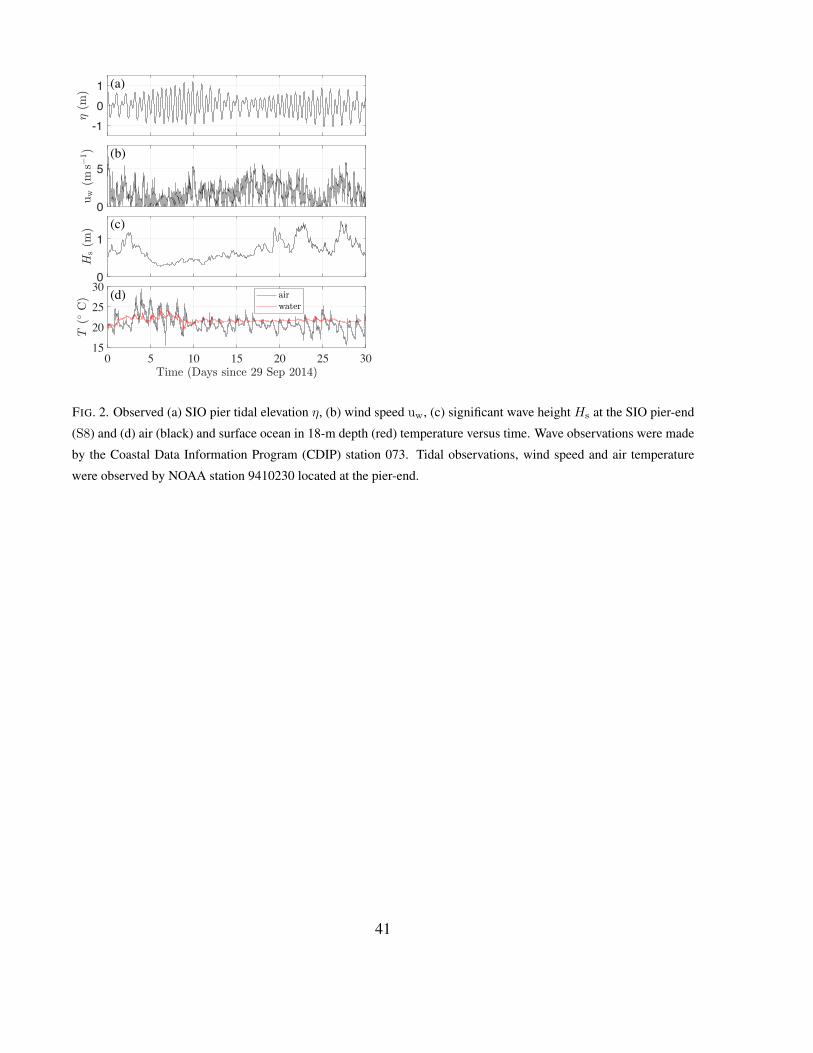
-101

2(m

)(a)

0

5

uw

(ms!

1) (b)

0

1

Hs(m

) (c)

0 5 10 15 20 25 30Time (Days since 29 Sep 2014)

15

20

25

30

T(/

C) (d) air

water

FIG. 2. Observed (a) SIO pier tidal elevation η, (b) wind speed uw, (c) significant wave height Hs at the SIO pier-end

(S8) and (d) air (black) and surface ocean in 18-m depth (red) temperature versus time. Wave observations were made

by the Coastal Data Information Program (CDIP) station 073. Tidal observations, wind speed and air temperature

were observed by NOAA station 9410230 located at the pier-end.

41

FIG. 3. Temperature versus vertical location below the mean tide level (MTL) z and time at cross-shore locations (a)

x = −100 m, h ≈ 2 m, denoted S2 (b) x = −155 m, h ≈ 4 m, denoted S4 (c) x = −219 m, h ≈ 6 m, denoted

S6 (d) x = −273 m, h ≈ 8 m, denoted S8 (e) x = −657 m h ≈ 18 m, denoted S18. The vertical axes have been

scaled to approximate the depth at each cross-shore location (the vertical scale of plot (e) is compressed to fit on the

page). Data in plots (a-d) have been removed (white) when sensors were inoperative or above the water line. Black

dots (right side, all panels) indicate the fixed (relative to MTL) thermistor locations. The black triangle in (e) indicates

the surface following sensor (surface level η shown as black line). Gray squares at the bottom of (e) indicate the arrival

time of isolated events highlighted in section 4, and colored squares indicate the arrival time of events A-D (left to

right) which are highlighted in detail in section 4. The black bar on the abscissa indicates the time span highlighted in

Figure 4.

42

FIG. 4. Similar to Figure 3, but with the time axes of all plots zoomed to highlight 3.5 days of internal wave activity.

The black bar on the abscissa indicates the timespan included in Figure 5.

43

FIG. 5. Similar to Figure 4, but with the time axes of all plots zoomed to highlight 9 hours beginning on 7 October

2014 00:15 PDT. The black bar on the abscissa indicates the timespan included in Figure 6

44

FIG. 6. Similar to Figure 5, but with the time axes of all plots zoomed to highlight 1.5 hours beginning on 7 October

2014 at 5:49 PDT. The 18.1◦C, 19.6◦C and 21.1◦C isotherms are highlighted with a black curve in all panels.

45

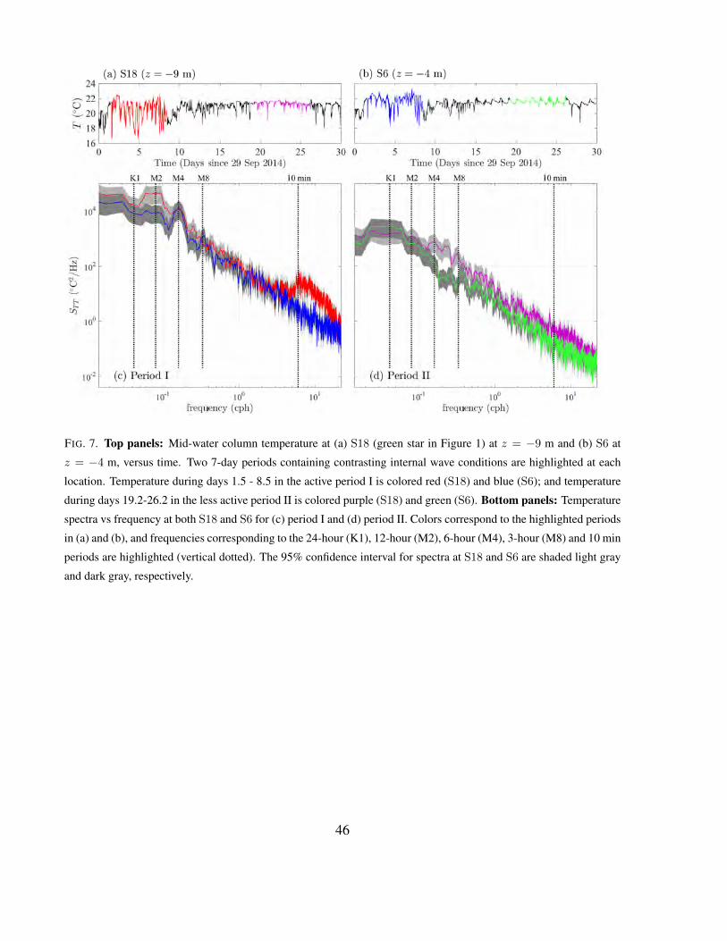
FIG. 7. Top panels: Mid-water column temperature at (a) S18 (green star in Figure 1) at z = −9 m and (b) S6 at

z = −4 m, versus time. Two 7-day periods containing contrasting internal wave conditions are highlighted at each

location. Temperature during days 1.5 - 8.5 in the active period I is colored red (S18) and blue (S6); and temperature

during days 19.2-26.2 in the less active period II is colored purple (S18) and green (S6). Bottom panels: Temperature

spectra vs frequency at both S18 and S6 for (c) period I and (d) period II. Colors correspond to the highlighted periods

in (a) and (b), and frequencies corresponding to the 24-hour (K1), 12-hour (M2), 6-hour (M4), 3-hour (M8) and 10 min

periods are highlighted (vertical dotted). The 95% confidence interval for spectra at S18 and S6 are shaded light gray

and dark gray, respectively.

46

FIG. 8. Five-hour time series of a NLIW runup event at S8 beginning at 8:13 am PDT on 26 October 2014: (a) S8

1 Hz temperature from near surface to near bed, (b) Cross-shore baroclinic current U ′ and (c) alongshore baroclinic

current V ′ versus depth and time. In (b) and (c), the bed and mean tidal surface are indicated by the black and blue

curves respectively.

47

FIG. 9. NLIW event example bottom temperature versus time beginning at 8:13 am PDT on 26 October 2014 for (a)

the cross-shore locations and (b) the pier-end (S8) alongshore locations (red dots in Figure 1a), offset by 0.1◦C in both

(a) and (b) for visibility. Gray dots indicate the event arrival time at all locations and open circles in (a) indicate the

temperature change that defines ∆T , with S8 ∆T = 1.26◦C indicated. The NLIW event ∆T was below the 0.15◦C

cutoff threshold onshore of the runup extent xR = −137 m, indicated by the dotted lines in (a).

48

S8 S6 S4

0

2

4

6

8

10

12

14

N

1:5/C < " T

1:0/C

< "T <

1:5/C

0:5/C

< "T <

1:0/C

0:3/C

< "T <

0:5/C

0:15/C < "T < 0:3/C

No Event

FIG. 10. Number (N ) and ∆T distribution (shading) of NLIW events observed between 9 and 30 October 2014 at

cross-shore locations S8, S6 and S4 (highlighted in Figure 1b). Of the N = 14 events observed at S8, only six were

observed at S4, and none with ∆T > 1.5◦C.

!40/!30/

!20/!10/0/10/

20/

30/

40/

0

0.02

0.04

0.06

0.08

cf (m s!1)

3

(a)

0

0.02

0.04

0.06

0.08

0.1

c gc=

h11!

z IW ~ h

2g

0 zIW

i 1=2

(ms!

1)

0 0.02 0.04 0.06 0.08 0.1cf (m s!1)

(b)

FIG. 11. (a) NLIW event front speed cf (radial direction) and incident angle θ at S8 for the 14 observed events between

9 and 30 October 2014. Events are plotted as if a viewer were looking offshore from the end of the SIO pier. (b) NLIW

two-layer gravity current front speed cgc versus event front speed cf (10) for the 14 NLIW events observed at S8. The

root-mean-square error is 0.016 m s−1, squared correlation R2 = 0.44, and the best-fit slope is 1.15.

49

19.5

20

20.5

21

21.5

22

22.5T

(o C o

ffset

by

0.1)

(a)

x = -55 mx = -73 mx = -100 m (S2)x = -118 mx = -137 mx = -155 m (S4)x = -173 mx = -191 mx = -218 m (S6)x = -246 mx = -273 m (S8)

0 1 2 3 4 5Time (hours from 12 Oct 2014 7:37 PDT)

18

18.5

19

19.5

20

20.5

21

21.5

22

T (o C

offs

et b

y 0.

1)

(b)

y = 200 my = 100 my = 0 my = -100 my = -200 m

FIG. 12. Bottom temperature versus time beginning at 7:37 on 12 October 2014 for (a) cross-shore locations and

(b) alongshore locations (as in Figure 9) offset by 0.1◦C for visibility. Gray dots indicate the arrival of a NLIW

cold pulse propagating with nearly zero angle onshore to xR = −137 m. Gray crosses indicate a second NLIW

pulse superimposed on the first, propagating at high angle from south to north. This second pulse caused significant

(≈ 0.8◦C) temperature reduction in water as shallow as 1 m (x = −55 m).

50

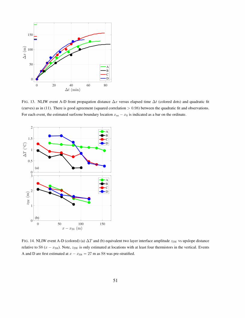
0 20 40 60 80"t (min)

0

50

100

150

"x

(m)

ABCD

FIG. 13. NLIW event A-D front propagation distance ∆x versus elapsed time ∆t (colored dots) and quadratic fit

(curves) as in (11). There is good agreement (squared correlation > 0.98) between the quadratic fit and observations.

For each event, the estimated surfzone boundary location xsz − x0 is indicated as a bar on the ordinate.

0

0.5

1

1.5

2

"T

(/C)

(a)

ABCD

0 50 100 150x! xS8 (m)

0

1

2

3

z IW

(m)

(b)

ABCD

FIG. 14. NLIW event A-D (colored) (a) ∆T and (b) equivalent two layer interface amplitude zIW vs upslope distance

relative to S8 (x− xS8). Note, zIW is only estimated at locations with at least four thermistors in the vertical. Events

A and D are first estimated at x− xS8 = 27 m as S8 was pre-stratified.

51

0

0.2

0.4

0.6

0.8

1"

T="

T0

(a)

ABCD

0 0.2 0.4 0.6 0.8 1"x="xR

0

0.2

0.4

0.6

0.8

1

z IW

=zIW

0

(b)

ABCD

FIG. 15. NLIW event A-D (colored) (a) normalized temperature anomaly ∆T/∆T0 and (b) normalized zIW/zIW0

versus normalized upslope propagation distance ∆x/∆xR. The linear fit (dotted black) to events A-D in (a) has

squared correlation R2 = 0.58. The linear fit to all events in (b) has slope -0.56 (dotted black) and R2 = 0.89. Note,

zIW is only estimated at locations with four thermistors in the vertical.

52

0 0.02 0.04 0.06 0.08 0.1cf0 (m s!1)

0

0.02

0.04

0.06

0.08

0.1c g

c 0=

h11!

z IW

0~ h

0

2g0 0z I

W0

i 1=2

(ms!

1)

(a)

ABCD

0 0.5 1 1.5 2 2.5df (#10!5 m s!2)

0

0.5

1

1.5

2

2.5

dgc

=1 2g0 0s

z IW

0~ h

0

11!

z IW

0~ h

0

2(#

10!

5m

s!2)

(b)

FIG. 16. (a) The best-fit gravity current speed cgc (10) versus NLIW front speed cf0 (11) at x0 with rms error of

0.013 m s−1 and best-fit slope 1.17. (b) Best-fit upslope gravity current deceleration dgc (12) versus NLIW front

deceleration df (11) with rms error of 0.2× 10−5 m s−2 and best-fit slope of 0.84 Both (a) and (b) are for events A-D.

0 50 100 150 200 250Observed "xR (m)

0

50

100

150

200

250

"x

R=

1 2c2 f0

=dob

s(m

)

(a)

ABCD

0 50 100 150 200 250Observed "xR (m)

0

50

100

150

200

250

"x

R=

1 2c2 gc

=dgc

(m)

(b)

FIG. 17. Predicted NLIW event A-D (colored) propagation distance ∆xR versus observed ∆xR using (a) best fit front

velocity cf0 at x0 and deceleration df , and (b) two layer gravity current velocity cgc and deceleration dgc. The rms

error is (a) 13 m and (b) 102 m.

53

0 0.2 0.4 0.6 0.8 1"x="xR

0

0.2

0.4

0.6

0.8

1z I

W(x

)=h(x

)ABCD

FIG. 18. NLIW event A-D (colored) normalized zIW/h versus upslope propagation distance ∆x/∆xR.

0

50

100

"PE

[Jm!

2] (a)

0

2

4

6

8

N2

[s!

2]

#10-4

(b)

0

2

4

6

8

S2

[s!

2]

#10-4

(c)

0 1 2 3 4 5Time (hours from 26 Oct 2014 8:13 PDT)

10-2

10-1

100

101

Ri

(d)

FIG. 19. Five hour time series during event C at S8 of (a) potential energy (5) change from tf1 (b) squared mid-water

buoyancy frequency N2, (c) squared mid-water shear S2, and (d) the gradient Richardson number Ri = N2/S2. All

values have been lightly smoothed (5-min filter) for visibility. Dotted lines in (a-c) indicate measurements recorded

before the arrival of the event front. The critical Richardson value (0.25) in (d) indicates the where shear-driven mixing

is expected.

54