Applied Numerical Mathematics 3 (1987) 347-360 North-Holland

347

OBSERVATIONS ON AN ADAPTIVE MOVING GRID METHOD FOR ONE-DIMENSIONAL SYSTEMS OF PARTIAL DIFFERENTIAL EQUATIONS *

Linda R. PETZOLD Computing and Mathematics Research Division, Lawrence Livermore National Laboratory Livermore, CA 94550, U.S.A.

Recently a scheme has been proposed for choosing a moving mesh based on minimizing the time rate of change of the solution in the moving coordinates for one-dimensional systems of PDEs. In this paper we show how to apply this idea to systems where the time derivatives cannot be solved for explicitly, writing the moving mesh equations in an implicit form. We give a geometrical interpretation of the scheme which exposes some of its weaknesses, and suggest some modifications based on this interpretation which increase the efficiency of the scheme. Finally, we present some numerical experiments which illustrate how well the resulting method works.

1, Introduction

In this paper we describe some observations on an adaptive moving mesh method for

one-dimensional partial differential equations (PDEs) and suggest some improvements to in- crease its efficiency and extend its range of applicability. The resulting scheme is easy to understand, efficient, and can be applied to a wide range of problems.

Several authors have proposed schemes which move the mesh to follow and/or resolve steep wave fronts. One class of methods [l-4] moves the mesh to equidistribute or approximately equidistribute a given mesh function such as the arc length of the solution. Another class of methods [5-71 moves the mesh so that in the transformed coordinates the solution varies less rapidly in time. This latter approach requires a regridding strategy to insert or delete or move nodes to resolve the spatial gradients, but it appears to result in fewer time steps for problems with very steep fronts. It is the second approach that we will study here.

A difficulty with the schemes introduced in [5-71 is that to determine the equation which moves the mesh they require the system to be written in a special form. For example, in [6,7], the system must be written as u, + v 9 G(u) = S, and in [5] as u, = f( u, uX, u,,). While this is no trouble for many classes of important problems, it is not always possible or convenient to write the equations in a standard form as above. Many systems of physical interest are naturally written in a form where the time derivatives are not so easily isolated. There may be several time derivatives in one equation, and other equations may have no time derivatives at all (see for example [8,9]).

In this paper we show how to apply the idea of moving the mesh to minimize the time rate of change in the moving coordinates to systems where the time derivatives cannot be solved for

* This work was performed under the auspices’of the U.S. Department of Energy by Lawrence Livermore National Laboratory under contract no. W-7405-Eng-48.

0168-9274/87/$3.50 0 1987, Elsevier Science Publishers B.V. (North-Holland)

348 L. R. Petzold / Adaptive moving grid method

explicitly. We present a geometrical interpretation of the scheme when it is applied to a scalar PDE which suggests some modifications which improve its efficiency. We discuss how to scale the scheme so that it can be applied to poorly scaled systems, and give other details of our implementation such as the time integration strategy and static rezone strategy. Finally, we present some numerical experiments which illustrate how well this scheme works.

2. Moving mesh equations

One of the difficulties in solving a system of PDEs with a moving front on a nonmoving grid is that, as the front passes through a grid point, the solution at that grid point changes very rapidly. When this happens, it is necessary to use very small time steps to retain accuracy. Because there are usually many grid points that the front needs to pass through (especially in problems such as combustion modelling, where the front must be resolved to maintain accuracy), this constant need for small time steps can slow down a calculation enormously. If the mesh points are moving, but more slowly than the front, as happens in equidistrihution strategies, then a similar problem can occur.

A solution to this problem is to move the grid points at the speed of the front or, more generally, to move the grid so that in the transformed coordinates the solution is changing as slowly as possible. A moving grid scheme is given in [5] which accomplishes this for the system

u,=f(u, u,, u,,). We derive this scheme here for again for completeness. Transforming coordinates to a moving grid system, (1) becomes

ii- u,i = j-(14, ux, u,,). (2) The grid velocity Z? is chosen to minimize the time rate of change of u and x in the new coordinates. Thus J? satisfies

min[ ~~ti/12+oLII~l12] = min[&i2+~-~2] k k

= min ~(f(u)+~,.t)~+*i~]. A 1

Here, (Y is a positive scaling parameter. The sum is over the number of PDEs. This quadratic in R can be minimized at each mesh point, leading to the equation given in [5],

- . f(

x= u, uxr uxx ) l 4

ff + u, l u, 9

where the dot product is over the number of PDEs. Equations for moving the mesh in two or three dimensions are derived similarly.

For equations which are not written in the form (l), it may be inconvenient or impossible to identify f and hence to apply (4) to move the mesh. To overcome this difficulty, the moving mesh equations can be written in a form which does not depend on f explicitly. Consider the genera! equation

qu,, u, u,, u,,) = 0. (5)

L. R. Petzold / Adaptive moving grid method 349

Let UT, be the time derivative of the solution at a nonmoving mesh point xj. Then, changing variables to a moving coordinate system, we have

+ u, + u,k

Now we proceed as before. minimking the time rate of change of u and X,

min[ IIti112+allRl12] = min[xti2+01R2] i 2

(6)

= min[~(u,+u*i)2+ai2]. 2 0)

Solving this quadratic in i at each mesh point for the minimum gives

(u,+ux~)‘u,+(Y~=o, (8)

but by (6) this gives

ark+timu,=O. (9)

This implicit form of the moving mesh equation is applicable to systems of the general form (5), and it reduces to (4) for systems of the form (2) in exact arithmetic. These ideas can be extended in a straightforward way to two dimensions.

3. Geometrical interpretation and modified moving mesh equation

We can obtain some intuition about what the moving mesh scheme is doing by looking at a geometric derivation of it for a scalar PDE. Then it is easy to see how it can be modified slightly to remove some of its weaknesses and make it even more efficient.

Consider a moving front which is illustrated at time t, by the solid line in Fig. 1. The tangent line I, bassing through a given point (& uJ’> at grid point Xj and time t, on the solution curve is given by

u - ui” = u,(x -xi”). 00)

The line I, passing through (x;, uy) which is orthogonal to Zr is given by

u-u;= -(x-xi”)& (11)

Let (x7+*, uy+r ) be the point on 1, which intersects the solution at time t,+r. Then (xT+r, ~7”) satisfies

n+l uj (

n+l - ui”= - xj - x;)/ux.

Now in the limit as t,, I - t, + 0, (12) becomes . U= - k/U, 9

(12)

or rewriting,

g+u;li=o,

which is the same equation (where at = 1) that we derived in Section 2.

(1 ) 3

350

U

I,. R. Petzold / Adaptive moving grid method

T- 'i" J

)$+1

X

Fig. 1. Geometrical interpretation of moving mesh equation.

Thus we see that in the limit as t,, 1 - t, + 0 for a single PDE, the moving mesh equation (9) moves a given mesh point xi along the line segment which is orthogonal to the solution at (Xi, Uj) until it intersects the solution at the next time.

This strategy minimizes the change in u and X, but it may not necessarily lead to the largest possible time step, because the mesh points can easily cross. Consider a very steep moving front as in Fig. 2. The mesh point at j moves at a velocity which is nearly equal to the speed of the front, while the mesh point at j + 1 doesn’t move because the solution has no gradient there. Thus the time steps must be made very small to prevent the mesh points from colliding.

U

d

xn+l j-k1

n+l I u.

I+1

- u(t,) --- la,,, 1

JJ i I xn+l

I: j I u;“)

r{

* ( k x;+, , u” -P

I+1 1 X

Fig. 2. Mesh point crossing problem.

L.R Petzold / Adaptive moving grid method 351

We have dealt with this difficulty by adding a penalty function to the minimization in deriving the moving mesh equations which tries to give nearby nodes nearly equal velocities. Thus we find

for X > 0, which leads to

i

.

Qstj + lij . Uxj + X atj-iZj_1 ij+* - Xj

- Xj_*)' - (Xj+* - Xj)2 I = Om ( xi (15)

As it is written above, the moving mesh equation is not invariant under scalings and translations of u and x. In the next section we show how to derive a weighted moving mesh equation which overcomes this problem. One way of looking at the effect of the penalty term is as an extra diffusion or smoothing term to the mesh velocity (not the solution of the equations). If we had started with an equally spaced mesh, x! - xi-1 = xi+ 1 - xj, then the added term approximates X(A),,. Thus we might think of it as diffusing the mesh velocity. It smooths out differences in the mesh velocity to try to keep mesh points from crossing. It does not entirely eliminate mesh point crossings, but in our experience it has been quite effective in eliminating mesh point crossings as a significant source of difficulties in a calculation.

The penalty term in (15) is important even though mesh points are deleted and moved apart by the regridding strategy after every time step. With the penalty term, the method can take larger time steps, because mesh points are not so likely to cross within a time step.

4. Implementation details

TO be useful, this scheme requires a strategy to adjust the mesh point locations and to add or delete mesh points after every time step to resolve the spatial gradients. It needs a method for advancing the time steps, and a means of dealing with poorly scaled problems.

For the rezone after each time step, we have used the dual reconnecting grid strategy described in [5]. We outline it here. First, a reference mesh is determined which cquidistributes a mesh function based on the first and second deriva&s of the solution. The reference mesh is chosen so that locally,

Ax I] u, I] + (Ax)’ 11 u,, II = TOL < TOL, (16)

where TOL is a user-defined error tolerance, and the number of mesh points is the smallest number which is needed to satisfy the tolerance. In practice, to avoid needless interpolations due to minor chattering, we change the number of mesh points only if it goes up by at least ten percent or down by at least twenty percent. The reason behind this particular choice of mesh function is that since we do not know in advance what equations we will be solving or how they are differenced, a linear combination of Ax ]I u, I] and ( Ax2) II u,, I] can be regarded as some crude measure of the error. We find the equidistributing mesh approximately by inverse interpolation of the integral of the mesh function, where the mesh function m(x) is given by

m(x) = II ux II +@&c II 4, II 9 where bc~ the local optimal mesh spacing, is determined by solving the quadratic equation (16) locally for x.

352 L R Petzold / Adaptive moving grid method

It is possible to interpolate the solution from the old mesh directly onto the reference mesh, but we have avoided this approach because it would in general require interpolating every mesh point on each step, and each interpolation introduces some error into the solution. Instead, we use “le dual reconnecting grid approach, which is a compromise between choosing the best mesh, and avoiding needless interpolations. At the beginning of each time step, there is one dual grid point per reference zone. Then the solution and the grid are advanced using the moving mesh equation (15). A new reference mesh is then generated to satisfy (16). Finally, grid points are added or deleted so that there is exactly one grid point per reference zone, and grid points at the edge of zones which are too close to other grid points are moved apart. This scheme has worked well in practice, and on most time steps requires few interpolations of grid points because the locations of most grid points are not changed during the rezone. The interpolations are accomplished by means of the PCHIP package of monotone interpolation codes by Fritsch and Carlson [lo]. In principle, it should be possible to apply a similar dual reconnecting grid strategy in two dimensions.

Many problems from practical applications are not nicely scaled. Both the moving mesh equations and the static rezone method need to be scaled to compensate for this. We would like the method to be, as nearly as possible, invariant under scalings and translations 3 = ax + b, 1) u = cu + d. In the moving mesh scheme, if we derive the moving mesh equation to minimize instead a weighted I, norm,

N+l

I] ii ]I: = x (iii/wi)*, where ii = ( uT, x)~, i=l

N lii,jU,i j c stj

Wf

’ +a- 4-x i E 1 4+*

N is the number of PDEs in the original system, and wi are weights which we will soon specify, then the resulting moving mesh equation at Xj is given by

i

Zj-ij_1 ij+l - ij

- I = 0.

( Xj - Xj-1)' (xj+l - xj)2

(17)

The weights wi are chosen to be

wi =max(l~i,--Ei,~], floor(i)), i=l, 2 ,..., N+ 1, (18) where Ei,_ is the maximum of the Ith component of ii over all mesh points, and Ei,kh is the minimum of Ei over all mesh points. It is easy to check that if floor(i) is scaled appropriately, the moving mesh equation (17) is invariant under scalings and translations of u and X. The choice of floor(i) can be important, however, especially for components which start out initially flat and later develop gradients. It is worth noting that the parameters cy and X in (17) are, in contrast to the earlier equation (15), now dimensionless. In all of our numerical experiments, including the experiments in the next section, we chose (Y = 1 and X = 0.2. The choice QL = 1 was made because it leads to the minimum of I] i ]I, and thus the largest time step given a simple stepsize selection strategy, in the absence of mesh point crossings. The choice X = 0.2 was made because it appears to result in the best performance, based on the author’s experience, over a wide range of problems. Thus the values of the parameters should be considered to be, for practical purposes, problem-independent.

How the system of PDEs coupled with the moving mesh equation is formulated in the code is an important consideration. Writing the equations in a diffeieirt but analytically equivalent form

L.R. Pettold / Adaptive moving grid method 353

can sometimes lead to a very ill-conditioned matrix in the linear system which is s&red at every time step, resulting in substantially more time steps. These effects are entirely due to roundoff error. Considering for simplicity the PDE (1) coupled with the moving mesh equation (a), we can formulate this system in the implicit form as

ir - u,i = f (u, UX? UJ, R+u;ir=O,

or explicitly as (19

lJ - u,R -f (u, ux, UJ, . x=- f( u, ux9 u,,) l u,/(l + U,’ Uxjr

or, substituting for i in (20a) from (20b), in a totally explicit form,

(204

(2W

fi=fh ux9 Ux,b-U,Cf(U9 ux, U,,)%/(1 +uxmu,)),

k= -f(u, ux, UXJ l %/O + V%). 121)

While these formulations are all equivalent analytically for the explicit PDE (11, the implicit and totally explicit formulations (19) and (21) give much better results than (20). The difference is due to matrix ill-conditioning and is especially pronounced for problems with extremely steep fronts. By writing out the iteration matrices for (19), (20), and (21), we can see that when 1 U, 1

for some nodes is large compared to other terms in the iteration matrix, the iteration matrix of (20) has a much larger condition number than that of (19) or (21), causing the poor results. An example will be given in the next section which illustrates this problem. We do not know whether this is a source of difficulty for moving mesh schemes other than the one that we have studied here.

In the numerical experiments in the next section, the PDEs including the extra term u,x,, coupled with the moving mesh equation (17), were discretized in space using first-order centered differences for U, and u,,. This yields a large system of differential/algebraic equations (DAE). The system is not in standard ODE form because there are now several time derivatives in each equation. We solved this system with the DAE solver DASSL [ll], which uses variable-stepsize variable-order backward differentiation formulas to advance the solution in time. DASSL was restarted with the first-order method after every rezone (after nearly every time step). An option was specified to have DASSL attempt for the time step after a restart the stepsize that it would have used on the next step had there been no restart. This is necessary because the default time step on a restart would otherwise be unreasonably small, which would lead to some misleading statistics as well as long run times.

DASSL is not an optimal choice of solver for this application, for several reasons. Because there are so many restarts, the solver has no chance to increase the order and is almost always using the backward Euler method, with variable stepsize. Secondly, for stiff systems there is a small nonstiff transient after each restart, because of errors introduced in the interpolation phase

of the rezone. The error estimate in DIASSL is not designed with this situation in mind. Nonetheless, it has performed satisfactorily, although not surprisingly there is evidence in the statistics that the code is slower than necessary because of these types of difficulties. However, it is not our purpose in this paper to discuss the design of a DAE solver which is appropriate for

adaptive moving mesh calculations. We are currently considering this problem and will report on it in a future paper.

354

5. Numerical experiments

L.R. Petzold / Adaptive moving grid method

In this section we present two scheme.

numerical examples which illustrate the effectiveness of this

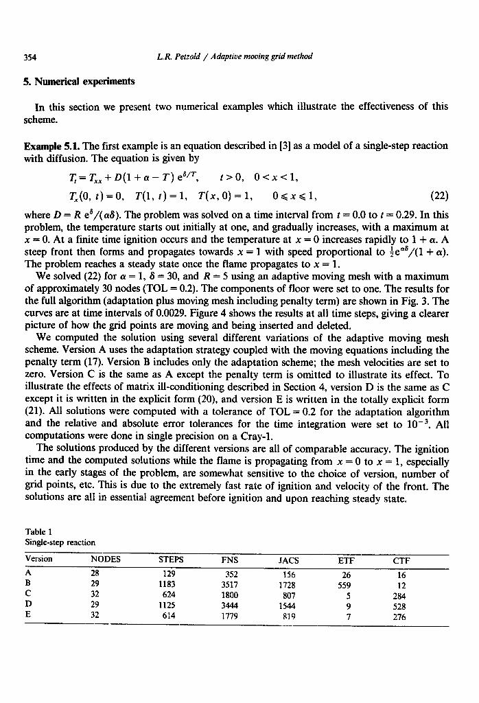
Example 5.1. The first example is an equation described in [3] as a model of a single-step reaction with diffusion. The equation is given by

q = T,. + D(l + (Y - T) es/T, 00, O<X<l,

T,(O, t)=O, T(l, t)=l, T(x,O)=l, O<xal, (22) where D = R es/( (~8). The problem was solved on a time interval from t = 0.0 to t = 0.29. In this problem, the temperature starts out initially at one, and gradually increases, with a maximum at x = 0. At a finite time ignition occurs and the temperature at x = 0 increases rapidly to 1 + QL. A steep front then forms and propagates towards x = 1 with speed proportional to ie”“/(l + cw). The problem reaches a steady state once the flame propagates to x = 1.

We solved (22) for (Y = 1, 6 = 30, and R = 5 using an adaptive moving mesh with a maximum of approximately 30 nodes (TOL = 0.2). The components of floor were set to one. The results for the full algorithm (adaptation plus moving mesh including penalty term) are shown in Fig. 3. The curves are at time intervals of 0.0029. Figure 4 shows the results at all time steps, giving a clearer picture of how the grid points are moving and being inserted and deleted.

We computed the solution using several different variations of the adaptive moving mesh scheme. Version A uses the adaptation strategy coupled with the moving equations including the penalty term (17). Version B includes only the adaptation scheme; the mesh velocities are set to zero. Version C is the same as A except the penalty term is omitted to illustrate its effect. To illustrate the effects of matrix ill-conditioning described in Section 4, version D is the same as C except it is written in the explicit form (20), and version E is written in the totally explicit form (21). All solutions were computed with a tolerance of TOL = 0.2 for the adaptation algorithm and the relative and absolute error tolerances for the time integration were set to 10B3. All computations were done in single precision on a Cray-1.

The solutions produced by the different versions are all of comparable accuracy. The ignition time and the computed solutions while the flame is propagating from x = 0 to x = 1, especially in the early stages of the problem, are somewhat sensitive to the choice of version, number of grid points, etc. This is due to the extremely fast rate of ignition and velocity of the front. The solutions are all in essential agreement before ignition and upon reaching steady state.

Table 1 Single-step reaction

Version NODES STEPS FNS JACS ETF CTF

A 28 129 352 156 26 16 B 29 1183 3517 1728 559 12 C 32 624 1800 807 5 284 D 29 1125 3444 1544 9 528 E 32 634 1779 819 7 276

-

L. R. Petzold / Adaptive moving grid method 355

0.0 0.1 0.2 0.3 0.4 0.5 0.6 0.7 0.8 U" .., 1

axial position

Fig. 3. Single-step reaction with adaptive moving mesh.

The results of the computation using the four different schemes are presented in Table 1. In the table, NODES is the maximum number of grid points used by the code over all time steps, STEPS is the number of time steps needed to complete the problems, FNS is the number of function evaluations that DASSL used, JACS is the number of Jacobian evaluations, ETF is the number of times the time step was reduced due to a failure of the error test in DASSL, and CTF is the number of times the time step was reduced due to failure of the Newton iteration in DASSL to converge.

356 L. R. Petzold / Adaptive moving grid method

M .

0

3.3 0.1 0.2 0.3 0.4 0.5 0.6 0.7 0.8 0.9

axial posk,tLon

Fig. 4. Single-step reaction at all time steps.

It is apparent from Table 1 that the penalty term is very helpful in decreasing the number of time steps by preventing nodes from coming too close together. Version A with the penalty term took approximately five times fewer time steps than version C without that term. It is clear that matrix ill-conditioning can be a significant problem if the equations are formulated in the wrong way; version C using the implicit formulation (19) of the moving mesh equations and version E using the totally explicit formulation (21) required roughly half as many time steps as version D,

L. R Petzold / Adaptive moving grid method 357

which used the explicit formulation (20). All of the versions were faster than not using a moving mesh, and the implicit moving mesh with penalty term computed the solution using approxi- mately one tenth as may time steps as the version with no moving mesh.

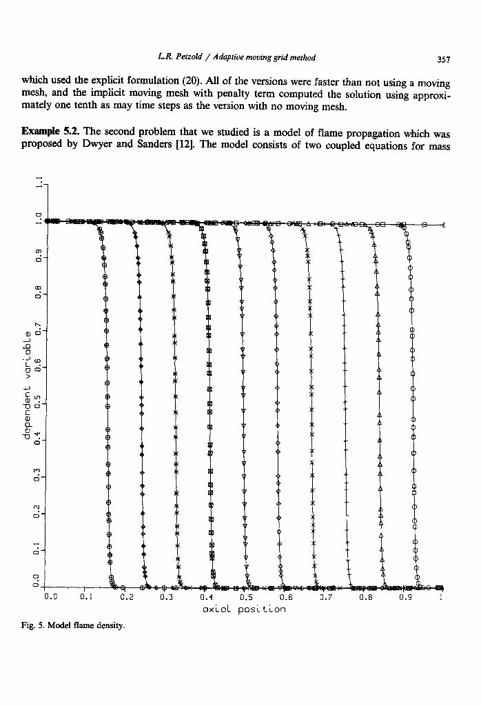
Example 5.2. The second problem that we studied is a model of flame propagation which was proposed by Dwyer and Sanders [12]. The model consists of two coupled equations for mass

n I

>:

>(

x x

x

x x

)(

)(

x

>c

X

>:

x

8

x

x

x

t I - - 0.0 0.1 0.2 0.3 0.4 0.5 0.6 0.7 0.8 0.9 1

axial position

c

Fig. 5. Model flame density.

358 L. R. Petzold / Adaptive moving grid method

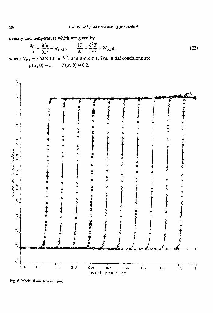
density and temperature which are given by

ap= 3% aT i12T

at ax* --PDF& at= -+&#I

3X2

where NDA = 3.52 X 106 ee41T, and 0 < x < 1. The initial conditions are

P(X, 0) = 1, T( x, 0) = 0.2.

0.0 0.1 0.2 0.3 0.4 0.5 0.6 0.7 0,8 0.9

axial position

Fig. 6. Model flame temperature.

L. R. Petzold / Adaptive moving grid method 359

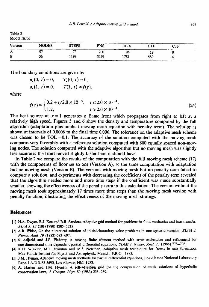
Table 2 Model flame

Version

A B

NODES STEPS

57 73 56 1193

FNS JACS ETF CTF

2oc 96 19 9 3559 1781 589 ,pi

The boundary conditions are given by

P,(O, 1) = 0, q(o, t) = 0,

P,(L t) = 09 T(l, t) = j(t), where

f0 t { 0.2 + t/2.0 x 10-4, t < 2.0 x = 10-4,

1.2, t >, 2.0 x 10-4.

The heat source at x = 1 generates a flame front which propagates from right to left at a relatively high speed. Figures 5 and 6 show the density and temperature computed by the full algorithm (adaptation plus implicit moving mesh equation with penalty term). The solution is shown at intervals of 0.0006 to the final time 0.006. The tolerance on the adaptive mesh scheme was chosen to be TOL = 0.1. The accuracy of the solution computed with the moving mesh compares very favorably with a reference solution computed with 600 equally spaced non-mov- ing nodes. The solution computed with the adaptive algorithm but no moving mesh was slightly less accurate; the front moved slightly faster than it should have.

In Table 2 we compare the results of the computation with the full moving mesh scheme (17) with the components of floor set to one (Version A), TV the same computation with adaptation but no moving mesh (Version IS). The versions with moving mesh but no penalty term failed to compute a solution, and experiments with decreasing the coefficient of the penalty term revealed that the algorithm needed more and more time steps if the coefficient was made substantially smaller, showing the effectiveness of the penalty term in this calculation. The version without the moving mesh took approximately 17 times more time steps than the moving penalty function, illustrating the effectiveness of the moving mesh strategy.

mesh version with

References

111

PI

PI

VI

PI

161

H.A. Dwyer, R.J. Kee and B.R. Sanders, Adaptive grid method for problems in fluid mechanics and heat transfer, AIAA J. 18 (10) (1980) 1205-1212. A.B. White, On the numerical solution of initial/boundary value problems in one space dimension, SIAM J. Numer. Anal. I9 (1982) 683-697. S. Adjerid and J.E. Flaherty, A moving finite element method with error estimation and refinement for one-dimensional time dependent partial differential equations, SIAM J. Numer. Anal. 23 (1986) 778-796. K.H. Winkler, M.L. Norman and M.J. Newman, Adaptive mesh techniques for fronts in star formation, Max-Planck-llnstitut fur Physik und Astrophysik, Munich, F.R.G., 9983. J.M. Hyman, Adaptive moving mesh methods for partial differential equations, L,os Alamos National Laboratory Rept. LA-UR-82-3690, Los Alamos, NM, 1982. A. Harten and J.M. Hyman, A self-adjusting grid for the computation of weak solutions of hyperbolic conservation laws, J. Comput. Phys. 50 (1983) 235-269.

360 LR. Petzold / Adaptive moving grid method

[7] E.J. Kansa, D.L. Morgan and L.K. Morris, A simplified moving finite difference scheme: Application to dense gas dispersion, SIAM J. Sci. Statist. Comput. 5 (3) (1984) 667-683.

[S] M.E. Coltrin, R.J. Kee and J.A. Miller, A mathematical model of the coupled fluid mechanics and chemical kinetics in a chemical vapor deposition reactor, J. Electrochem. Sot. 131 (2) (1984) 425-434.

[9] R.J. Kee, L.R. Petzold, M.D. Smooke and J.F. Grcar, Implicit methods in combustion and chemical kinetics modeling, in: J. Brackbill and B. Cohen, eds., Multiple Time Scales (Academic Press, New York, 1985) 113-144.

[lo] F. Fritsch and R. Carlson, PCHIP final specifications, UCID-30194, Lawrence Livermore National Laboratory, Livermore, CA, 1982.

[ll] L.R. Petzold, A description of DASSL: A differential/ algebraic system solver, in: R.S. Stepleman, ed., Transactions on Scientific Computation I (IMACS, 1982).

[12] H.A. Dwyer and B.R. Sanders, Numerical modeling of unsteady flame propagation, Sandia National Laborato- ries Livermore Rept. SAND77-8275, Livermore, CA, 1978.