Observer-based Fault Detection and Identification for Rotating Machinery

Haedong Jeong, Seungtae Park, and Seungchul Lee*

UNIST

Contents

• Rotating Machinery

• Model-based FDI

• FDI for Rotating Machinery

• Case Study

• Conclusion

2

Contents

• Rotating Machinery

• Model-based FDI

• FDI for Rotating Machinery

• Case Study

• Conclusion

3

Rotating Machinery

• Key component

– Safety and efficiency issues

• Prognostics and Health Management (PHM)

– Data-driven Method (Machine Learning)

– Model-based FDI (Fault detection, isolation and identification)

4

PHM

Hardware Redundancy

Analytic Redundancy

Output Estimation

Parity SpaceParameter Estimation

Observer

UnsupervisedLearning

SupervisedLearning

Data-driven Model-based

Residual Generation

Contents

• Rotating Machinery

• Model-based FDI

• FDI for Rotating Machinery

• Case Study

• Conclusion

5

• Analytic Redundancy

• Residual

– A quantitative difference between target system and mathematical model

– Observer-based residual estimation

Model-based FDI

6Chen, J., & Patton, R. J. (2012). Robust model-based fault diagnosis for dynamic systems (Vol. 3). Springer Science & Business Media.

nonzero if fault existsresidual =

0 if no fault

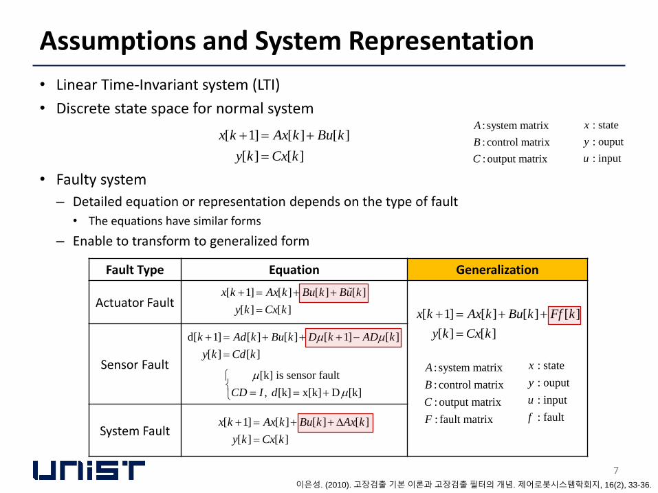
Assumptions and System Representation

• Linear Time-Invariant system (LTI)

• Discrete state space for normal system

• Faulty system

– Detailed equation or representation depends on the type of fault

• The equations have similar forms

– Enable to transform to generalized form

7

[ 1] [ ] [ ]

[ ] [ ]

x k Ax k Bu k

y k Cx k

: system matrix

: control matrix

: output matrix

A

B

C

: state

: ouput

: input

x

y

u

Fault Type Equation Generalization

Actuator Fault

Sensor Fault

System Fault

[ 1] [ ] [ ] [ ]

[ ] [ ]

x k Ax k Bu k Bu k

y k Cx k

d[ 1] [ ] [ ] [ 1] [ ]

[ ] [ ]

k Ad k Bu k D k AD k

y k Cd k

[ 1] [ ] [ ] [ ]

[ ] [ ]

x k Ax k Bu k Ax k

y k Cx k

[k] is sensor fault

, [k] x[k] D [k]CD I d

[ 1] [ ] [ ] [ ]

[ ] [ ]

x k Ax k Bu k Ff k

y k Cx k

: system matrix

: control matrix

: output matrix

: fault matrix

A

B

C

F

: state

: ouput

: input

: fault

x

y

u

f

이은성. (2010). 고장검출기본이론과고장검출필터의개념. 제어로봇시스템학회지, 16(2), 33-36.

Observer-based Residual Generation

• Faulty system

• State estimation via Observer

– Output estimation error (Residual)

• Relation between residual and fault signal

8

[ 1] [ ] [ ] [ ]

[ ] [ ]

x k Ax k Bu k Ff k

y k Cx k

ˆ ˆ ˆ[ 1] [ ] [ ] ( [ ] [ ])

ˆ ˆ[ ] [ ]

x k Ax k Bu k L y k Cx k

y k Cx k

ˆ : state estimation

ˆ : ouput estimation

: observer gain

x

y

L

1

0

ˆe[ 1] [ 1] [ 1]

ˆ( [ 1] [ 1])

[ 1]

C ( ) [ ] [ ]

( ) [0] ( ) [ ]k

k q

q

k y k y k

C x k x k

C k

A LC k Ff k

C A LC A LC Ff k q

Residual

ˆWhen [ 1] [ 1] [ 1]

( ) [ ] [ ]

k x k x k

A LC k Ff k

Observer-based Residual Generation

• Normal case

– The residual value converges to zero-value

• Faulty case

– The residual value converges to specific shape

9

2

0.099 0.011 0 0[ 1] [ ] [ ] [ ]

0.009 0.999 0.009 0.009

[ ] 0 1 [ ]

56.139 0.602 , [ ] , [ ] 5sin( )T

x k x k u k f k

y k x k

L x k R u k k

[ ] 0f k [ ] 4cos( )f k k

1

0

e[ 1] ( ) [0] ( ) [ ]k

k q

q

k C A LC A LC Ff k q

Fourier Decomposition for General Faults

• Fourier Series

– Decompose a function of time into the frequency domain

• General fault signal– Modeling as Fourier series with unknown coefficient

10Lucas V. Barbosa, https://en.wikipedia.org/wiki/Fourier_transform#/media/File:Fourier_transform_time_and_frequency_domains_(small).gif

2

exp expn n

nkR j j

N

Radius PhaseSinusoid

per frequency

2 1

2

2[ ] exp exp

N

n n

n N

nkf k R j j

N

2 1

2

2[ ] exp exp

2 1 2 0 2 1exp exp exp

N

n n

n N

nkf k R j j

N

j k j k j kN N N

2 2 1 1 0 0 1 1 2 2where exp( ) exp( ) exp( ) exp( ) exp( )T

R j R j R j R j R j

• State estimation error

• Output estimation error

Fault Projection Matrix

11

1

0

1

ˆ[ 1] [ 1] [ 1]

( ) [ ] [ ]

( ) [0] ( ) [ ]

ˆ( ) [0] [ ]

[ ]

kk q

q

k

k x k x k

A LC k Ff k

A LC A LC Ff k q

A LC k

k

2 1 2 1

1 1 1 1 1 1

1 1 0 0 1 1

1 1

1 0

ˆ [ ] ( ) ( ) ( ) ( ) ( ) ( )

2 1 2 1[ ] exp ( ) ( ) exp (

j k j kN Nk k kk e I T I T F I T I T F e I T I T F

k j k I T F I T F j k I TN N

1

1) when

2[ ] : fault projection matrix, where exp ( )n

F k

nk T j A LC

N

1

ˆe[ 1] [ 1] [ 1]

ˆ( [ 1] [ 1])

[ 1]

ˆ( ) [0] [ ]

[ ] when

k

k y k y k

C x k x k

C k

C A LC C k

C k k

Recursive Fault Parameter Estimation

• The linear relationship

– Least Square Estimation (LSE) can be used

– The object function and solution

12

e[ 1] where [ ]k kk M M C k

2

1

min e[ 1]n

n k

k

k

J k M

1 1ˆ ˆ ˆ(e[k] )k k k k kK M

Simon, D. (2006). Optimal state estimation: Kalman, H infinity, and nonlinear approaches. John Wiley & Sons.

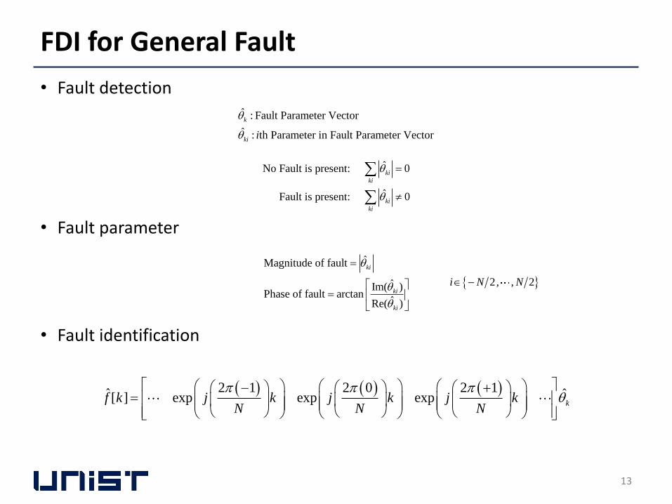
• Fault detection

• Fault parameter

• Fault identification

FDI for General Fault

13

ˆNo Fault is present: 0

ˆFault is present: 0

ki

ki

ki

ki

ˆMagnitude of fault

ˆIm( )Phase of fault arctan

ˆRe( )

ki

ki

ki

2, , 2i N N

ˆ : Fault Parameter Vector

ˆ : th Parameter in Fault Parameter Vector

k

ki i

2 1 2 0 2 1ˆ ˆ[ ] exp exp exp kf k j k j k j kN N N

Contents

• Rotating Machinery

• Model-based Fault Detection and Identification(FDI)

• FDI for Rotating Machinery

• Case Study

• Conclusion

14

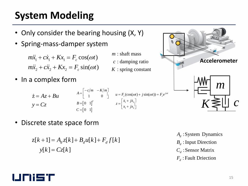
• Only consider the bearing housing (X, Y)

• Spring-mass-damper system

• In a complex form

• Discrete state space form

System Modeling

15

z[ 1] [ ] [ ] [ ]

[ ] [ ]

d d dk A z k B u k F f k

y k Cz k

:System Dynamics

: Input Direction

:Sensor Matrix

: Fault Driection

d

d

d

d

A

B

C

F

1 1 1

2 2 2

cos( )

sin( )

c

c

mx cx Kx F t

mx cx Kx F t

z Az Bu

y Cz

Accelerometer : shaft mass

: damping ratio

: spring constant

m

c

K

m

K c

1 0

0 1

0 1

T

c m K mA

B

C

1 2

1 2

(cos( ) sin( )) j t

c cu F t j t F e

x jxz

x jx

Contents

• Rotating Machinery

• Model-based Fault Detection and Identification (FDI)

• FDI for Rotating Machinery

• Case Study

• Conclusion

16

Case Study 1

• Fault detection and identification

17

[ ] 0.08exp( ) 0.05exp( )exp( ) 0.15exp( )exp( 2 ) 0.1exp( )exp( 2 )8 6 4

f k j k j j k j j k j j k

6 25[ ] 100 where 2

1000

jj k

u k e e

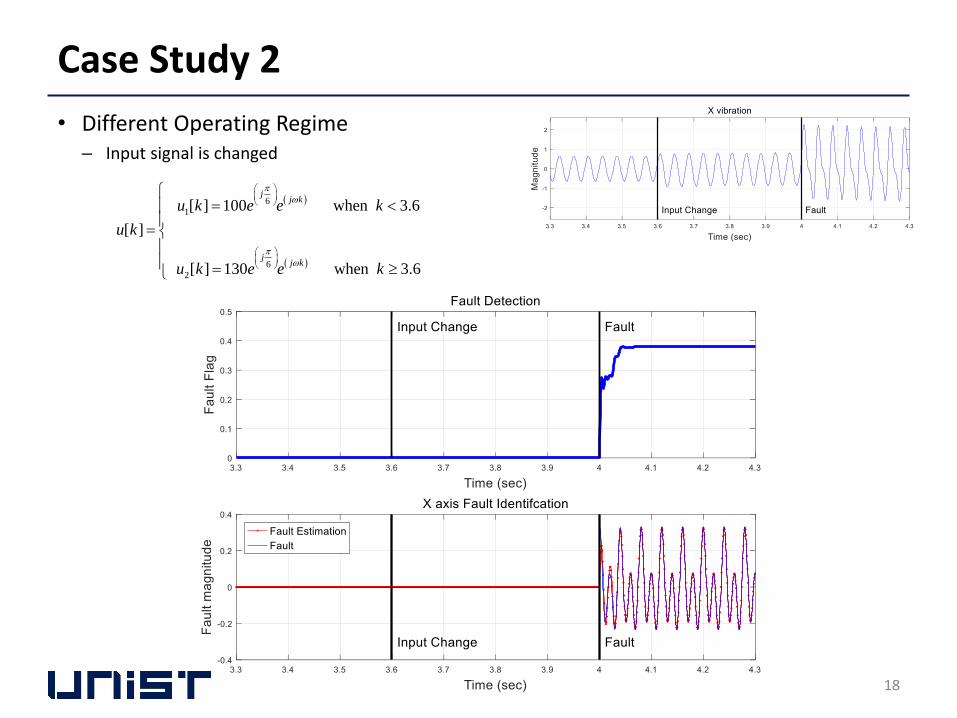
Case Study 2

• Different Operating Regime– Input signal is changed

18

6

1

6

2

[ ] 100 when 3.6

[ ]

[ ] 130 when 3.6

jj k

jj k

u k e e k

u k

u k e e k

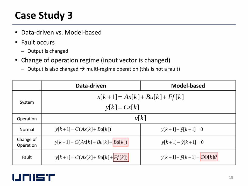
• Data-driven vs. Model-based

• Fault occurs– Output is changed

• Change of operation regime (input vector is changed)– Output is also changed multi-regime operation (this is not a fault)

Case Study 3

Data-driven Model-based

System

Operation

Normal

Change of Operation

Fault

19

[ 1] [ ] [ ] [ ]

[ ] [ ]

x k Ax k Bu k Ff k

y k Cx k

[ 1] ( [ ] [ ])y k C Ax k Bu k

ˆ[ 1] [ 1] [ ] y k y k C k

[ ]u k

ˆ[ 1] [ 1] 0y k y k

[ 1] ( [ ] [ ] [ ])y k C Ax k Bu k Ff k

ˆ[ 1] ( [ ] [ ] [ ])y k C Ax k Bu k Bu k ˆ[ 1] [ 1] 0y k y k

Case Study 3

• Data-driven vs. Model-based

– Under stationary condition

• Observation (Normal) VS Observation (Fault)

• Observation (Fault) VS Fault signal

– Fault detection problem

• Classification problem

20

Dat

a-d

rive

nFD

I

[ 1] [ 1]

( [ ] [ ] [ ])d d d

y k Cx k

C A x k B u k F f k

ˆ[ 1]f k

Signal

Ob

serv

atio

n(N

)O

bse

rvat

ion

(F)

Fau

lt

Case Study 3

• Data-driven vs. Model-based

– Under non-stationary condition (or Transient)

• 1) : The normal state

• 2) : Although the fault occurs, the state is transient

• 3) : The fault state

21

5k

5 8k

8k

Case Study 3

• Data-driven vs. Model-based

– Under non-stationary condition (or Transient)

• 1) : The normal state

• 2) : Although the fault occurs, the state is transient

• 3) : The fault state

22

5k

5 8k

8k

Case Study 4

• Proposed method

– Deterministic study

– But the method can be applied for the stochastic case

• Reduction of the number of basis in the fault projection matrix

• Effect of low-pass filter

23

[ ]k

1 1 1 1 1

2 1 0 1 2

2 2 2 1 2 1 2 2[ ] exp ( ) exp ( ) ( ) exp ( ) exp ( )k j k I T F j k I T F I T F j k I T F j k I T F

N N N N

2 1 2 1

1 1 1

1 0 1[ ] ( ) ( ) ( )j k j k

N Nk e I T F I T F e I T F

The number of basis is determined by sampling rate

Low frequency

Conclusion

• Model-based FDI is introduced

– Observer-based residual estimation

• The fault projection matrix is defined for FDI

• Proposed FDI method is validated through simulation

– 4 case studies

• Future work

– Include uncertainty into model (Modeling error, disturbance)

• Kalman filtered FDI or Unknown input observer-based FDI

– Implementation on testbed

24