Obuda University

PhD Thesis

Drive Control Optimization of Walker Robots

Using Dynamic Simulation Model

by

Istvan Kecskes

Supervisor:

Dr. Peter Odry, College Professor

Applied Informatics and Applied Mathematics

Doctoral School

Budapest, 2018

Members of the Defense Committee:

Members of the Comprehensive Examination Committee:

Date of the Defense:

Abstract

The high-quality energy-efficient regulation of electromechanical systems is an important chal-

lenge for today’s robot technology development. The construction of the dynamic simulation

model is indispensable to the optimization of robot driving controlling, because such a model

estimate adequately the robot’s behavior. The main aspects of the controlling’s quality can be

defined as: fast, energy efficient, battery saver, and ensure vibration-free walking for the robot.

The Szabad(ka)-II hexapod robot with 18 DOF embedded mechatronic devices is suitable for

complex drive control research. My goals also included achieving robustness concerning robot,

environmental and controller parameters since the mechanical and electronic inaccuracy of the

device is not negligible.

Model validation: During the verification and validation of the simulation model, I evaluated

whether the results of the simulation correspond to the real system. The validation procedure

was performed twice, first before the development and optimization of the drive control, then

afterwards, using a selected optimal controller. The former was necessary to develop the optimal

drive control using a realistic model. The latter was required to prove that the goal had been

achieved. For the classification of the validation results, the tolerances and expected error limits

were defined based on the measurement and estimation of system accuracy. During validation,

the motor current showed a significant difference, therefore this issue was discussed in detail.

Determining the main steps of the robot model validation and the numerical and qualitative

grading of the differences are the main scientific results.

Optimizer algorithm: Since the simulation tasks to be run were rather time-consuming, the

efficiency of the optimization algorithm had become a key issue. Algorithms able to find the op-

timum with the lowest number of function calls for multi-variable, non-continuous, non-linear,

mixed-integer problems were used. Heuristic search methods were tested against each other

on quick test functions which incorporate properties similar to those of a robotic simulation

problem. The best results were achieved by the particle swarm optimization method (PSO),

the implementation of which had been paralleled. A new and widely usable method was created

to select the most appropriate optimization search method.

Robust Multi-Objective Multi-Scenario Optimization: In general, quality motor control

needs respond to a number of requirements (such as low power consumption, accuracy, speed,

battery saving), so the system is multi-objective. The simulation model includes environmental

or mission parameters that are not part of the parameters to be optimized but their variation

creates different scenarios. A multi-scenario simulation can be created with the typical values

of these parameters where the optimum is searched for all scenarios at the same time. Such

optimum is more robust than one achieved through a process using separate scenarios since the

intended use of the robot is represented by the multi-scenarios.

Fuzzy Logic Motor Controller: A fuzzy-PI motor controller that can be embedded in the

processor of real robot was developed and optimized using the simulation model. A lookup

table-type solution for the real time operation of the fuzzy controller suitable in the low power

microcontrollers was developed. The feedback of the motor current to the fuzzy controller al-

lowed the option of providing control characteristics that avoid high current-torque fluctuations.

This ensures a softer control behavior or, in extreme cases, inverse directional control, which

can better protect the electromechanic parts and the batteries. This control behavior can be

easily implemented using fuzzy descriptive (linguistic) rules. By measuring the quality of the

motor controller, it was checked that the elaborated fuzzy-based control provided better quality

and robustness compared to the classic PID control.

In case of the Szabad(ka)-II robot, the presented drive optimization achieve 27% faster locomo-

tion and 10% less power consumption compared to an earlier, non-optimized program.

Keywords: Hexapod Robot, Dynamic Model, Fuzzy Logic Control, Robust Optimization, Multi-

Objective Optimization

Abstract

Az elektromechanikai rendszerek minosegi energia-hatekony szabalyzasa a mai robot technologiai

fejlodes egyik fontos kihıvasa. A szimulacios dinamikai modell megepıtese elengedhetetlen,

hiszen a robot hajtas szabalyzast egy olyan modszerrel lehet optimalizalni, amely jol meg-

becsulni a robot viselkedeset. A minosegi szabalyzas fo szempontjai ıgy hatarozhato meg:

gyors, energia-hatekony, akkumulator kımelo, razkodas-mentes jarast biztosıt a robotnak. A

Szabad(ka)-II hatlabu robot, 18 szabadsagfokos beagyazott mechatronikai eszkoz, alkalmas

osszetett hajtas szabalyozasi feladatok kutatasara. Emellett a robot- a kornyezet- es a szabalyzo-

parameterekkel szembeni robusztussag is a kutatasom celjai koze tartozik, mivel az eszkoz

mechanikai es elektronikai pontatlansaga nem elhanyagolhato.

Modell validalas: A szimulacio modell verifikalasa es validalasa alatt felmertem, hogy a

szimulacio eredmenyei megfelelnek-e a valos rendszernek. A validacios eljarast ketszer lett

elvegezve, eloszor a hajtas-szabalyozas fejlesztese es optimalizalasa elott, majd az utan, egy

kivalasztott optimalis szabalyzoval. Az elsore azert volt szukseg hogy egy valosaghu modellen

keressuk az optimalis szabalyzast. A masodik pedig igazolja, hogy valoban megvalosıtottam-

e a kituzott celt. A validalas eredmenyek klasszifikaciojahoz meghataroztam a toleranciakat

illetve varhato hibahatarokat a rendszer pontossaganak a kimerese es becslese alapjan. A

validacio soran a motor arama lenyeges elterest mutatott, ezert reszletesen foglalkoztam ezzel

a kerdeskorrel. A robot modell validalas fo lepeseinek meghatarozasa es az elteresek szamszeru

es minosegi osztalyozasa a fo tudomanyos eredmenyek.

Optimalizalo algoritmus: Mivel idoigenyes szimulacios feladatokat kell futtatni az opti-

malizalo algoritmus hatekonysaga kulcskerdesse valt. Olyan algoritmusok lettek kivalasztva,

amelyek a legkevesebb fuggvenyhıvassal kepesek ratalalni az optimumra sok-valtozos, nem

folytonos, nem-linearis, vegyes egeszszamu problema eseten. Heurisztikus modszereket versenyeztet-

tem gyors tesztfuggvenyeken, amelyekbe ilyen hasonlo tulajdonsagok lettek beepıtve, mint ami

a robot szimulaciora is jellemzo. A reszecskeraj modszert (PSO) erte el a legjobb eredmenyt,

amelynek implementaciojat parhuzamosıtottam. Egy uj es szeleskorben alkalmazhato modszert

kaptam a legjobb optimalizacios kereso algoritmus meghatarozasara.

Robusztus tobbcelu tobbszcenarios optimalizalas: Altalaban a minosegi szabalyzas tobb

szempontnak is meg kell, hogy feleljen (peldaul kis fogyasztas, pontossag, gyorsasag, akku-

mulator kımeles), ezert a rendszer tobb-celu (multi-objektıv). A szimulacios modell tartal-

maz olyan kornyezeti vagy kuldetesi parametereket, amelyek nem tartoznak az optimalizalando

parameterekhez, de ezek valtozasa kulonfele szcenariot kepez. Ezen parameterek tipikus ertekeivel

egy tobb-szcenarios szimulaciot lehet letrehozni, ahol az optimum egyszerre minden szcenariora

van keresve. Az ilyen optimum robusztusabb mint ha csak egy szcenariora lenne keresve a

megoldas, hiszen a robot rendeltetesszeru hasznalatat a kivalasztott tobb szcenario reprezentalja.

Fuzzy-alapu motorszabalyzas: A szimulacios modellezes segıtsegevel fejlesztettem es opti-

malizaltam egy fuzzy-PI motor szabalyzot, amely beagyazhato a valos robotba. A kis tel-

jesıtmenyu mikrovezerloknek megfelelo kereso tablas megoldast fejlesztettem ki a fuzzy szabalyzo

valos ideju futasahoz. A motor aramanak visszacsatolasa a fuzzy szabalyzoba lehetoseget kınalt,

hogy olyan szabalyzasi jelleget biztosıtsak, amely keruli a nagy aram-nyomatek ingadozasokat.

Evvel egy puhabb vagy extrem esetben inverz iranyu szabalyzasi jelleg kaphato, amely jobban

vedi az elektromechanikat, valamint az akkumulatorokat. A fuzzy leıro szabalyaival konnyen

lehet ezt a viselkedest implementalni. A szabalyozas minosegenek meresevel ellenorizve lett,

hogy a kidolgozott fuzzy alapu iranyıtas jobb minoseget es robusztussagot mutat a klasszikus

PID-hez kepest.

Szabad(ka)-II robot eseten a bemutatott hajtas optimalizalas 27%-kal gyorsabb es 10%-kal

kisebb energiafogyasztast tudott elerni egy korabbi nem optimalizalt programhoz kepest.

Acknowledgement

First and foremost, I would like to thank my loving Creator for making me a curious being who

loves to explore His creation and for giving me the opportunity to do this research.

I would like to express the appreciation to my research supervisor Dr. Odry Peter. With-

out his guidance and persistent help this dissertation would not have been possible.

I would also like to show gratitude to my committee, including Prof. Dr. Rudas Imre, Prof.

Dr. Horvath Laszlo, Dr. Vamossy Zoltan, Dr. Galambos Peter and Dr. Pletl Szilveszter. I

must also thank to head of my doctoral school, Prof. Dr. Galantai Aurel.

I thank Cambridge University Press for permission to include Chapter 2 of my dissertation,

which was originally published in Robotica Journal.

I would also like to thank the University of Dunaujvaros for their financial support granted

through the predoctoral fellowship. This work is supported by the EFOP-3.6.1-16-2016-00003

project. The project is co-financed by the European Union.

To my family: you should know that your support and encouragement is worth more than

I can express it on paper.

Contents

1 Introduction 1

1.1 Research Background . . . . . . . . . . . . . . . . . . . . . . . . . . . . . . . . . 1

1.2 Research Objectives . . . . . . . . . . . . . . . . . . . . . . . . . . . . . . . . . . 2

1.3 Document Overview . . . . . . . . . . . . . . . . . . . . . . . . . . . . . . . . . . 2

1.4 Szabad(ka)-II Hexapod Robot . . . . . . . . . . . . . . . . . . . . . . . . . . . . . 3

2 Simulation Modeling 10

2.1 Simulation and validation at other hexapods . . . . . . . . . . . . . . . . . . . . 10

2.2 Szabad(ka)-II Simulation Model . . . . . . . . . . . . . . . . . . . . . . . . . . . . 12

2.3 Model Validation . . . . . . . . . . . . . . . . . . . . . . . . . . . . . . . . . . . . 20

2.4 Comparison of Results and Interpretation of Differences . . . . . . . . . . . . . . 27

2.5 Discussion and Conclusion . . . . . . . . . . . . . . . . . . . . . . . . . . . . . . . 41

2.6 Theses Summary . . . . . . . . . . . . . . . . . . . . . . . . . . . . . . . . . . . . 44

3 Optimization Methods for Trajectory and Motor Controller 47

3.1 Introduction . . . . . . . . . . . . . . . . . . . . . . . . . . . . . . . . . . . . . . . 47

3.2 Selection of Optimization Methods . . . . . . . . . . . . . . . . . . . . . . . . . . 50

3.3 Fuzzy-PI Controller . . . . . . . . . . . . . . . . . . . . . . . . . . . . . . . . . . 54

3.4 Results and Comparison . . . . . . . . . . . . . . . . . . . . . . . . . . . . . . . . 59

3.5 Discussion and Conclusion . . . . . . . . . . . . . . . . . . . . . . . . . . . . . . . 60

3.6 Theses Summary . . . . . . . . . . . . . . . . . . . . . . . . . . . . . . . . . . . . 62

4 Multi-scenario Multi-objective Optimization of Fuzzy-PI Motor Controller 64

4.1 Introduction . . . . . . . . . . . . . . . . . . . . . . . . . . . . . . . . . . . . . . . 64

4.2 Multi-scenario Multi-objective Optimization . . . . . . . . . . . . . . . . . . . . . 64

4.3 Fuzzy-PI Motor Controller . . . . . . . . . . . . . . . . . . . . . . . . . . . . . . . 68

4.4 Results . . . . . . . . . . . . . . . . . . . . . . . . . . . . . . . . . . . . . . . . . . 71

4.5 Discussion . . . . . . . . . . . . . . . . . . . . . . . . . . . . . . . . . . . . . . . . 74

4.6 Theses Summary . . . . . . . . . . . . . . . . . . . . . . . . . . . . . . . . . . . . 75

5 Embedding Optimized Trajectory and Motor Controller 77

5.1 Introduction . . . . . . . . . . . . . . . . . . . . . . . . . . . . . . . . . . . . . . . 77

5.2 Software Architecture . . . . . . . . . . . . . . . . . . . . . . . . . . . . . . . . . 78

5.3 Fuzzy-PI Motor Controller Implementation . . . . . . . . . . . . . . . . . . . . . 80

5.4 Comparison Results of Original and Optimized Driving . . . . . . . . . . . . . . 82

5.5 Discussion and Conclusion . . . . . . . . . . . . . . . . . . . . . . . . . . . . . . . 84

5.6 Theses Summary . . . . . . . . . . . . . . . . . . . . . . . . . . . . . . . . . . . . 85

6 Conclusion 87

iv

References 89

.1 Appendix: Comparison of Szabad(ka)-II with similar robots . . . . . . . . . . . . 98

.2 Appendix: Details of Szabad(ka)-II Dynamic Model . . . . . . . . . . . . . . . . 100

v

1 Introduction

1.1 Research Background

Many universities, research centers and companies have been researching and developing robots

since the 1970s, although most of them are laboratory prototypes. Generally, the incoming

robots have a number of shortcomings, so there is still no widespread use in the industry: they

are slow and not energy-efficient, which would be important for a mobile robot De Santos et al.

(2007).

Energy efficient walker robot development focuses primarily on energy efficient motor drive

and optimal robot’s structure. Various energy-efficient approaches have been studied for multi-

legged robots, where they research to minimize electrical energy by optimizing the structural

parameters of the locomotion de Santos et al. (2009). A complete dynamic model is important

for the development of walker robots and its energy efficient optimization processes: Dynamic

stability was researched by four legged walker robots with different legs and gaits Lin and

Song (2001); neural network-controlled walker robot were optimized using a simulation model

Von Twickel et al. (2012); or the size of actuators are defined using dynamic model of six-legged

robot Carbone and Ceccarelli (2008a).

Fuzzy control of six-legged walker robots is a widespread solution that has been developed in

last 20 years. For example, Pratihar et al. (2000) optimized a fuzzy-based walk controller with

a genetic algorithm. Besides walker robots - such as Sakr and Petriu (2007), fuzzy controller

are also used for crawling robots too Wang et al. (2009). Robust controlling requirements can

be met by fuzzy solutions Tanaka et al. (1996). Fuzzy systems show benefit from the classical,

commonly used PID controllers Kecskes and Odry (2014). Fuzzy controllers have the ability

to comply robustly, i.e. they can produce better results in extreme conditions Kecskes et al.

(2017a). The fuzzy controller can be advantageous compared to other complex controllers,

considering the resource requirement Kecskes et al. (2015a). The advantages of fuzzy control

are outstanding in complex, more freedom structures (robots, especially mobile robots), because

the deduction of model-based controllers are cumbersome task to such robots.

The general definition of the quality of the 4, 6 and 8 legged walkers was not dealt with in

detail. The energy efficiency and speed are the two main quality aspects, but the other aspects

are usually explored in independently, such as vibration and self-defense mechanisms. Exam-

ining preferences between different quality aspects and Pareto solutions are future challenge

in research of walker robots. This dissertation was initiated to following this direction and its

main new scientific result relates to the definition of walking quality.

The Szabad(ka)-II hexapod robot with 3 degree of freedom per leg is an embedded mecha-

tronic system suitable for complex drive control tasks. Using a simulation model the robot’s

behavior in different applications can estimate, even in extreme cases: energy-efficient, vibration

free, or battery-saver drive controls can be developing. The behavior of the robot can be evalu-

ated in extreme cases, which is important because the protection against structural damage is

also included in the task of motor control.

1

1.2 Research Objectives

The main aim is to develop a motor control process based on an effective fuzzy controller that

is capable of controlling systems with a nonlinear dynamics and strong parameter uncertainty.

During the research, mechatronic tools are needed to embed, test, and validate the developed

procedures I have. The Szabad(ka)-II robot is such a device, described in next section 1.4.

Research objectives are follows:

• Build the complete mechatronic simulation model of the robot / manipulator. An elec-

tronically and dynamically realistic model, i.e. the embedded electric control, electric

motors, robot body and ground dynamics are all part of the model. Realistic, that is

sufficiently precise according to measurement errors. It is required to compare the results

generated by the robot / manipulator and the simulation model, and then interpret the

differences. If one of the variables differs more than the expected tolerance, then the

reasons and explanations must be sought.

• It should look for the appropriate, but inexpensive, sensor surface that is needed for

robot walking and drive control. Three dimensional digital accelerometer and gyroscope

mounted on robots can be used well in model validation and gait / walking tracking.

In addition to angular velocity encoders, the current of each drive motor can also be

measured, which can be an important input of the fuzzy controller. The measurement of

the power supply is also useful for validating the model.

• Define the drive quality metrics (objective functions) that can be used to achieve the de-

sired behavior and quantify the robot’s walking quality. Longer-term research purpose is

to determine the preference between the objective functions so that the quality measure-

ment will be appropriate for the various applications of the robot. This assumes that the

desired utility function, which aggregate the multi-objective quality based on preference,

and the drive optimum are sufficiently robust.

• It is necessary to define the gaits or walking tasks (scenarios) where the quality measure-

ment should be carried out, taking into account the objectives and the capabilities of the

robot. It need to choose scenarios that can be carried out in the simulation and in reality

in the given laboratory conditions.

• It should look for the optimal quality drive control according to the selected objective

functions, which includes the parameters of leg trajectory curve and fuzzy-based controller.

Optimization on the simulation model should be run simultaneously on all the specified

scenarios.

• The validation of the obtained drive optimum should be performed. For this, the optimal

controller and trajectory must be embedded in the robot and the measurements should

be made.

1.3 Document Overview

The dissertation is structured as follows.

2

• Chapter 1.4: Introduces the development objectives and motivations of the Szabad(ka)-II

hexapod robot. Describes the basic structural elements of the robot, and compares it to

another similar hexapod robots. Its content has been published in Kecskes et al. (2015b).

• Chapter 2: The realistic dynamic model is an essential element of the computational

optimization. First, the dissertation describes the simulation model and its validation

procedure. The measurements on the real robot are compared to the simulation results

in the validation procedure. A genetic algorithm is used to define the immeasurable

parameters in the model calibration tasks. Its content has been published in Kecskes

et al. (2015b).

• Chapter 3: The motor controllers are developed and optimized using the validated simu-

lation model. The fuzzy logic–based motor controller takes the error of joint angles and

the absolute motor current as the inputs, and produces proportional voltage output. This

chapter describes the selection of the global optimizer algorithm, and the design vari-

able definition related to the motor controller and trajectory curve. Its content has been

published in Kecskes and Odry (2014).

• Chapter 4: The quality definition and quantification of the hexapod robot’s walking are

analyzed as a multi-objective problem. The multi-objectives are aggregated into a scalar

fitness value using preference weights. The multi-scenario simulation approach in applied

to find the optimum for the intended use of the robot instead of a single scenario. In

this chapter, the optimization of a Fuzzy-PI motor controller is described, which can be

embedded in the low-cost microcontrollers on the Szabad(ka)-II robot.

• Chapter 5: The optimized motor controller and trajectory curve are implemented into an

improved real-time framework of the Szabad(ka)-II robot. The initial and the developed

leg-drive systems are compared. Its content has been published in Kecskes et al. (2016).

• Chapter 6: The overall conclusions of the previous chapters.

The research and development related to Szabad(ka) hexapod robot series are wider than the

scope of this dissertation. The parts of the research shown within the blue rectangle in Fig. 1.1

belong to the scope of the present thesis.

1.4 Szabad(ka)-II Hexapod Robot

Nowadays, due to the continuous development of technology, applications in the field of mobile

robotics are becoming increasingly common. Accordingly, researchers show more interest in

development of various mobile devices. The simplest mobile robots have wheels, crawlers or

a combination of these two. For these robots overcoming even small obstacles is difficult. In

contrast to wheeled devices, walker robots have more complex structures in terms of their me-

chanical, electrical and software composition, but when properly built they can easily overcome

much higher and more complex barriers.

Walker robots can be classified into bipeds, quadrupeds, hexapods, octopods and “cen-

tipedes”. With more than two-legged robot structures, it is easier to achieve and maintain

3

Figure 1.1: This Dissertation and the Szabad(ka) Hexapod Robot Series Research and Development

balance and the center of gravity – compared to the size of the robot – can be closer to the

ground than in the case of bipeds. With the right walking algorithm three noncollinear legs of

the robot are on the ground all the same time. Quadrupeds have a disadvantage over structures

with six or more legs namely that if they use a static stable gait then only one leg can be in air

at a time, which results in slow walking speed. Using a dynamic stable gait like the trot gait

two legs can be lifted at the same time, but in this case it is harder to respond to unforeseen

events like obstacle collision.

In case of hexapods, when the fast “tripod” gait is used, there are always three legs on the

ground, and three in the air. Therefore, the walking speed of a hexapod robot can be two or

three times faster than that of a quadruped robot. In case of octopods, due to the extra two feet,

robots can have four feet on the ground and four in the air in the same time, however, there is

a disadvantage, because it is difficult to touch the ground with four feet simultaneously. Eight-

legged robots have greater weight, power consumption and cost more because of the extra legs.

In Kar (2003), a detailed analysis of walking devices was carried out. This analysis separately

dealt with the maximal speed of the robots depending on the number of feet. The publication

Silva and Machado (2007) deals with the evolution of legged locomotion systems, and presents

different possibilities for the implementation. In Silva and Machado (2012) several optimization

examples and methods are presented for minimizing the energy consumption by modifying the

design and walking with evolutionary computation. A detailed classification of gaits was given

in Collins and Stewart (1993).

4

Based on the above, six legged construction is the most practical choice for a walking device.

Simpler wheeled robots are capable of overcoming obstacles with heights smaller than the

radius of their wheels. More advanced wheeled robots using for example the Rocker-Bogie

suspension, like the Curiosity robotic rover are of course able to roll over much higher obstacles.

Bipeds can overcome barriers to the height of their knees. Hexapod structures, depending on

their structural design, are suitable for walking on obstacles up to two to four times higher than

the length of their legs. The main disadvantage of hexapods, compared to the wheeled robots

is that they consume more power, and their walk is relatively uneven. Also, the top speed of

a hexapod is lower than the speed of a wheeled robot of the same size. Collins and Stewart

(1993) also discusses the walker robot’s ability to overcome obstacles.

1.4.1 Developmental Objectives of Szabad(ka) Robots

Applications of a hexapod walker potentially include reaching territories dangerous for humans,

to aid exploration, demining, rescuing, in industrial-, military-, terrestrial or other environments.

While developing Szabad(ka) robots the research objectives were: a) low-price (if necessary

single-use, e.g. tasks in radioactive or contaminated environment), b) optimal structural design

c) optimal walking algorithm for even and rough terrains.

In the case of my current robot, Szabad(ka)-II, the focus was on the dynamic modeling in

order to be able: a) to optimize the motor controlling and walking algorithms, b) to optimize

the robot structure. For these objectives walking on even ground was sufficient. Walking on

uneven ground will be a capability of my next robot, whose development has already started

and is based on the experience obtained from Szabad(ka)-II.

1.4.2 Szabad(ka)-II’s Structural and Mechatronical Properties

Szabad(ka)-II robot is the third robot in Szabad(ka) series. The first robot was made from

plastic (vitroplast), and it used 12 RC servos Odry et al. (2006); Appl-DSP.com (2011). The

second robot Szabad(ka)-I was made mostly from aluminum and was driven by 18 DC servo

motors equipped with planetary gearheads and encoders. It did not have a dynamic model and

its mechanical parameters were concluded using simple static calculations. Burkus and Odry

(2007)

Szabad(ka)-II Burkus et al. (2011) is a complex electro-mechanical system made from alu-

minum and steel. All of its legs have three degrees of freedom, i.e. three servo motors per leg

are used to drive the joints.

The torque transmission between the reductors and the joints was achieved with bevel

gears manufactured by company Maedler. These gears were reworked and adjusted to proper

dimensions. The module number of the bevel gears was determined through experiments.

The required loads used in the experiments were obtained from simulations. Based on the

simulations a 1:1 reduction value was assigned to the bevel gears at the two joints with smaller

loads, (Link1,Link3), while a 1:2 reduction at the joints with higher loads (Link2). The joints in

the body (Coxa-Thorax) use ball bearings (manufactured by SKF), and the joints in the legs

(Tibia-Femur and Femur-Coxa) use plain bearings (manufactured by IGUS).

The shafts on which the gears are mounted are held by the reductor with a single plain

bearing in the smaller reductors, and by a single ball bearing in the larger reductors. Based on

5

preliminary assessments, it was assumed that the shaft play appearing on the reductor shafts

will remain within appropriate limits so the reductors were mounted without using external

bearings for additional support. The reason behind this solution was to reduce size, weight

and complexity. It was subsequently found out that the problem was assessed incorrectly.

The imperfect solution resulted in a 2-3 degree backlash on the reductors’ axes. Because of this

drawback, in the construction of the next robot the single internal bearings will be supplemented

with external ones.

The innovations that were performed on Szabad(ka)-II (Fig. 1.2), the current IT system

and the plans connected to the software are detailed in Burkus et al. (2011). The robot’s micro-

controllers were selected based on the integrated peripheral requirements, previous experiences

and computational demands of the algorithms. The methods of the microcontroller selection

are explained in Burkus and Odry (2008).

The arrangement of the joints is shown in Fig. 1.2. The α joint is located in the body and

it can rotate the next segment in a horizontal plane. The other joints θ1 and θ2 are located in

the legs. These joints can rotate the next segment in a vertical plane.

Figure 1.2: The Szabad(ka)-II Hexapod Robot: Picture, Structure, and Names of Parts

Three kinds of Cartesian coordinate systems should be introduced for the robot kinematics:

1. World coordinate system – (XW , YW , ZW ), where theX−Y plane represents the horizontal

ground; Z axis is directed upward and the origin is at the initial point of the robot. This

coordinate system is shown in Fig. 1.2 in blue.

6

2. Coordinate system of robot body – (XR, YR, ZR), where X axis shows the front side of the

robot and the walking direction in case of straight movement; Z axis is directed upwards;

the origin is placed at the geometric center of the robot body. This is presented in Fig.

1.2 in yellow.

3. Coordinate system of robot legs – (X,Y, Z), where X axis is the leg’s starting direction

from the body; Z axis is directed to front side; the origin is placed in the center of the

first link (Link1). Coordinate system of robot legs depicted in black and shown in Fig.

1.2.

For Szabad(ka)-II, specific DC servo motors were selected from company Faulhaber Faul-

haber.com (2014). These motors are more efficient and have lighter weight than the motors

used in previous robot. The experience gained from the design and exploitation of Szabad(ka)-I

(Burkus and Odry (2008)) was used in the design process of Szabad(ka)-II.

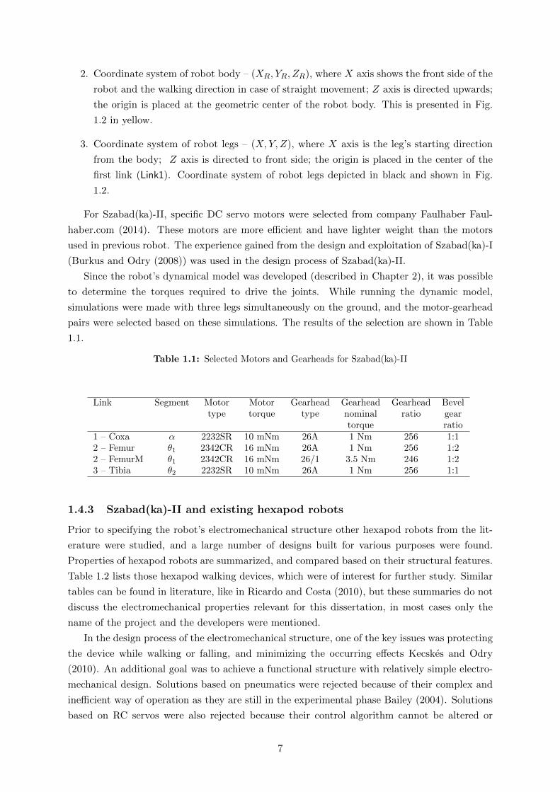
Since the robot’s dynamical model was developed (described in Chapter 2), it was possible

to determine the torques required to drive the joints. While running the dynamic model,

simulations were made with three legs simultaneously on the ground, and the motor-gearhead

pairs were selected based on these simulations. The results of the selection are shown in Table

1.1.

Table 1.1: Selected Motors and Gearheads for Szabad(ka)-II

Link Segment Motor Motor Gearhead Gearhead Gearhead Beveltype torque type nominal ratio gear

torque ratio1 – Coxa α 2232SR 10 mNm 26A 1 Nm 256 1:12 – Femur θ1 2342CR 16 mNm 26A 1 Nm 256 1:22 – FemurM θ1 2342CR 16 mNm 26/1 3.5 Nm 246 1:23 – Tibia θ2 2232SR 10 mNm 26A 1 Nm 256 1:1

1.4.3 Szabad(ka)-II and existing hexapod robots

Prior to specifying the robot’s electromechanical structure other hexapod robots from the lit-

erature were studied, and a large number of designs built for various purposes were found.

Properties of hexapod robots are summarized, and compared based on their structural features.

Table 1.2 lists those hexapod walking devices, which were of interest for further study. Similar

tables can be found in literature, like in Ricardo and Costa (2010), but these summaries do not

discuss the electromechanical properties relevant for this dissertation, in most cases only the

name of the project and the developers were mentioned.

In the design process of the electromechanical structure, one of the key issues was protecting

the device while walking or falling, and minimizing the occurring effects Kecskes and Odry

(2010). An additional goal was to achieve a functional structure with relatively simple electro-

mechanical design. Solutions based on pneumatics were rejected because of their complex and

inefficient way of operation as they are still in the experimental phase Bailey (2004). Solutions

based on RC servos were also rejected because their control algorithm cannot be altered or

7

modified, for it is fixed Braunl (1998). In case of most other robots having at least three

DOF-s per legs, particular attention was paid to the development of the algorithms, while the

optimization of the electromechanical structure was less important. Most of the constructions

were relatively robust, and resulted in a cumbersome walk.

Detailed comparison of Szabad(ka)-II and other similar hexapod robots can be found in

Appendix .1.

Robot’s Name: Year: DOF/leg Description:

Tarry I 1992 3Simulates the walking of the stick insect. Uses RC

servos. Lewinger et al. (2005)

Robot I 1993 2Early mechanism to imitate cockroaches. Forms the

basis of Robot II, III. Center (2008)

TUM 1991 3Introduces a model of hexapod walking machine

following biological principles. Lewinger et al. (2005)

Robot II 1996 3Improved successor of Robot I. It uses 6 watt DC

motors. Center (2008)

Tarry II 1998 3Improved version of Tarry I. Also uses RC servos.

Lewinger et al. (2005)

Lauron III 1999 3DC motors, robust transmission using timing belts.

Celaya and Albarral (2003)

LAVA 1999 3Early differential gear system, driven by DC servo

motors. Zielinska and Heng (2002)

Biobot 2000 3Pneumatic drives, with a cockroach-like foot

structure. Delcomyn and Nelson (2000)

Hamlet 2001 3Complex mechanical solutions, driven by DC servo

motors. Fielding et al. (2001)

RHex 2001 0Intentionally simple structure, driven by 6 DC

motors. Saranli et al. (2001)

Robot III 2002 2–5Enhanced version of Robot III. It uses pneumatics.

Center (2008)

Sprawlita 2001 2Pneumatic structure imitating the cockroach’s gait.

Bailey (2004)

LEMUR II 2002 4Successor of LEMUR I. Uses DC servo motors with

harmonic drives. Kennedy et al. (2002)

Whegs I 2003 1“Wheel with legs” concept. Driven by 6 wheels with

rods. Allen et al. (2003)

Whegs II 2003 1 Improved version of Whegs I. Allen et al. (2003)

Lauron IV 2004 3Enhanced version of Lauron III, with optimized

mechanism. Regenstein et al. (2007)

Genghis II 2004 2Mechanically simple robot with only two degrees of

freedom. Porta and Celaya (2004)

8

AQUA 2004 1Swimming robot with paddles and one degree of

freedom per leg. Georgiades (2005)

BILL-Ant-p 2005 3Ant-like hexapod with RC servos, equipped with a

head and scissors. Lewinger et al. (2005)

Hexapod 2005 2The authors’ first prototype. Ant-like hexapod using

RC servos. Odry et al. (2006)

Gregor I 2006 2/3Cockroach-like robot, using RC servos. Arena et al.

(2006)

ATHLETE 2006 6Rolling or crawling robot, with six wheels. Has a

load capacity of 450 kg. Hauser et al. (2006)

SLAIR 2 2007 3Successor of SLIAR. Has a differential drive with

modified RC servos. Konyev et al. (2008)

ANTON 2007 3Successor of SLIAR 2. Without a differential drive,

with its own reductors. Konyev et al. (2008)

Szabad(ka)-I 2007 3

Hexapod using servo motors. Has reductors, its own

production encoders, and bevel gears for additional

reduction. Burkus and Odry (2008)

HexCrawler 2008 2Hexapod with RC servos and two degrees of freedom.

Janrathitikarn and Long (2008)

Chiara 2008 3/4Very elaborate hexapod using RC servos. Has two

front arms. CMU (2008)

Lynx. BH3-R 2008 3Axisymmetric construction using RC servos. Currie

et al. (2010)

SILO6 2008 3Robust robot, with differential drive, driven by servo

motors. Gonzalez de Santos et al. (2007)

Cassino 2008 3Low cost, hybrid hexapod robot operated by a PLC

with on-off logic. Carbone and Ceccarelli (2008b)

COMET-IV 2009 4Hexapod with hydraulic drive, large dimensions and

weight. Ohroku and Nonami (2008)

Szabad(ka)-II 2009 3

Successor of Szabad(ka)-I. Among others, the DC

servo motors, drives, encoders, and bevel gears were

enhanced. Burkus and Odry (2008)

Oscar 2009 3Self-reconfiguring axisymmetric hexapod robot using

RC servos. Jakimovski et al. (2009)

SpaceClimber 2011 4

A particularly advanced robot using brushless DC

motors and Harmonic Drive gears. Bartsch et al.

(2012)

Octavio 2012 3

Ultra lightweight multi-legged robot that consists of

up to eight isomorphic leg modules with an easy

snap-in system. Von Twickel et al. (2012)

Table 1.2: Comparison of Hexapod Robots

9

2 Simulation Modeling

My complete dynamical simulation-model realistically describes the real low-cost hexapod walker

robot Szabad(ka)-II within prescribed tolerances under nominal load conditions. This validated

model is novel, described in detail, for it includes in a single study: a) digital controllers, b)

gearheads and DC motors, c) 3D kinematics and dynamics of 18 DOF structure, d) ground

contact for even ground, e) sensors and battery model. In my model validation: a) kinematical-

, dynamical- and digital controller variables were simultaneously compared, b) differences of

measured and simulated curves were quantified and qualified, c) unknown model parameters

were estimated by comparing real measurements with simulation results and applying adequate

optimization procedures. The model validation helps identifying both model’s and real robot’s

imperfections: a) gearlash of the joints, b) imperfection of approximate ground contact model,

c) lack of gearhead’s internal non-linear friction in the model. Modeling and model valida-

tion resulted in more stable robot which performed better than its predecessors in terms of

locomotion.

2.1 Simulation and validation at other hexapods

The general usage of the simulation modeling in hexapod robot design are summarized in

Tedeschi and Carbone (2014).

The static verification of a proposed CAD model can more or less determine if a prototype

is viable, but is not sufficient to provide the optimal structure. That was the reason why the

dynamic simulation model of Szabad(ka)-II was created and validated. This kind of modeling

is also important in the development of a robot’s software like in the walking algorithm. Using

a real robot for testing is time consuming and creating various test environments is expensive.

In contrast to this, simulating the target scenarios can be much faster, cheaper and easier. Of

course, it is vital for the dynamic model to provide the adequate results.

From the 32 robots listed in Table 1.2, I found 7 robots (besides Szabad(ka) robots) having

a dynamic simulation model. Table 2.1 summarizes these dynamic models. In this research,

models without a real hardware device were not addressed; therefore these researches were not

included in Table 2.1. The study of dynamic models is more important than kinematic modeling

because Szabad(ka)-II also has a dynamic model. Purely kinematic models do not include those

critical parts which are studied here, such as the motor currents, forces, ground contact model,

gearhead efficiency, gearlash, etc. At the same time dynamic models in most cases contain all

kinematic parts: exact structure of the robot, joint limits, even or uneven ground, obstacles,

etc. It is worth mentioning that kinematic models are usually used for studying robot motion

or walking in various environments like in the case of the following real robots: LAVA Zielinska

and Heng (2002), Genghis II Porta and Celaya (2004), BILL-Ant-p Lewinger et al. (2005),

ATHLETE Hauser et al. (2006), COMET-IV Ohroku and Nonami (2008), Lynx.BH3-R Currie

et al. (2010).

There are a large number of robot simulators available, emphasizing different aspects of

robot simulation Von Twickel et al. (2012). The mentioned models are mostly integrated to the

10

Table 2.1: Simulation Models Comparison of Hexapod Robots

Real Robot’sName

Simulator Purpose of dynamic model Verification/Validation

RHex Saranliet al. (2001)

SimSect“assess the viability of the designthrough simulation studies”

“verify in simulation that thecontrollers of Section 3 are able toproduce fast, autonomous forwardlocomotion of the hexapod platform”

Sprawlita Bailey(2004)

ADAMS“expected observation for the controltrials is based on the results of thesimulated experiments”

“Simulated experiments are powerfultools for verifying expected results ofcomplicated animal experiments.” “Inany case, analyzing the behavior ofthe simulated robot system in the caseof partial sensor failure will certainlybe interesting.”

AQUAGeorgiades (2005)

Simulink“to develop simple gaits that wereimplemented on the robot”

“model was validated withexperiments: The match between thetwo sets of forces was good and itprovided the model validation thatwas sought”

ANTON Konyevet al. (2008)

Simulink

“Development and test of complexreal-time embedded systems consistsof many steps from modeling andsimulation of the plant till theimplementation of the source code inthe real hardware.”

“The results of simulation and theresults of real experiments arepractically identical.”

Cassino Carboneand Ceccarelli(2008b)

Simulink

“dynamics analysis can be carriedout in order to size the actuators fora leg module (Carbone, G. &Ceccarelli, M. 2004)”

none

SpaceClimberBartsch et al.(2012)

“precise visual comparison of thefoot behavior on the ground andbetter tuning of the ground contactparameters in the simulation”

“A comparison between the real robotand the simulated version wasperformed before the simulation wasused for locomotion parameteroptimization.”

OctavioVon Twickel et al.(2012)

YARS

“optimized using evolutionarytechniques together with a physicalsimulation of the machine and itsenvironment”

“tests on hardware are indispensableto validate that the identified controlprinciples are grounded in the physicalworld.” “it has to be sufficientlyprecise to allow transferability ofcontrollers from simulation tohardware with at least qualitativelycomparable behaviors” “Except for afew parameter changes controllersdeveloped in simulation weresuccessfully transferred to hardware.

Szabad(ka)-IBurkus and Odry(2008)

Simulink help the design of Szabad(ka)-II none

Szabad(ka)-IIBurkus et al.(2013)

Simulink optimize robot structure and control The subject of this paper

Matlab/Simulink simulator environment (Simulink Kecskes and Odry (2009a); Konyev et al.

(2008); Bailey (2004); Georgiades (2005); Currie et al. (2010), YARS Von Twickel et al. (2012),

ADAMS Bailey (2004), and SimSect Saranli et al. (2001)). The Szabadka robot models were

also implemented in Simulink, because I already had experience with motor controlling in this

environment.

The elaboration and quantification of the model validation does not exist in these studies,

11

i.e. the comparison between the simulation results and reality is rather descriptive, for example:

• In Von Twickel et al. (2012): “Comparison of performance in hardware and simulation

it has to be sufficiently precise to allow transferability of controllers from simulation to

hardware with at least qualitatively comparable behaviors”

• In Konyev et al. (2008): “The results of simulation and the results of real experiments are

practically identical.”

• In Georgiades (2005): “ . . . model was validated with experiments: The match between the

two sets of forces was good and it provided the model validation that was sought . . . ”

• In Zheng et al. (2013): “good agreement between the simulation and the experiment

results, the errors in the static process is very small (nearly zero) and some errors exist

in the dynamic process (less than 20%)”

• In Rone and Ben-Tzvi (2014): “The maximum error between the disk positions of experi-

mental results and the dynamic virtual power response steady-state component is 2.1961

% in disk 8”

The point in my trials was to quantify the simulation errors in order to be able to compare

different situations and parameters, and run the optimization to tune up certain parameters

of the model, similarly to the research in Bartsch et al. (2012). The Genetic Algorithm (GA)

method was selected to tune up such parameters in my model, since the evolutionary algorithms

are proven as effective solution in the robotic field Rudas and Fodor (2008).

The main aim of these simulation models is to evolve the walking gaits and controllers, like in

Von Twickel et al. (2012); Konyev et al. (2008); Saranli et al. (2001); Bailey (2004); Georgiades

(2005); Currie et al. (2010). Evolutionary robotics, neural controllers and optimization of pa-

rameters are usually developed in simulations. This is due to time and cost constraints, but tests

on hardware are indispensable to validate that the identified control principles are grounded in

the physical world Von Twickel et al. (2012). The attempt to implement the optimized walking

developed with the help of simulation into the real robot is not an unachievable ambition. The

following citation from Nelson et al. (2009) confirms this ambition: “Although developing an

experimental research platform capable of supporting the evolutionary training of autonomous

robots remains a non-trivial task, many of the initial concerns and criticisms regarding embod-

iment and transference from simulated to real robots have been addressed. There are sufficient

examples of evolutionary robotics research platforms that have successfully demonstrated the pro-

duction of working controllers in real robots [9-12]. Also, there have been numerous examples of

successful evolution of controllers in simulation with transfer to real robots [13-19].” This and

the results of the Octavio robot research Von Twickel et al. (2012) confirmed my endeavor to

use the validated simulation model for the development of the robot controller.

2.2 Szabad(ka)-II Simulation Model

This section describes the electromechanical (physical) modeling and simulation of the Szabad(ka)-

II hexapod walker robot. The model includes the kinematics and dynamics of the robot, and

12

Figure 2.1: Control layers of Szabad(ka) robot series, layers of Szabad(ka)-II are highlighted.

also the models of the DC motors and the control electronics. Just like in the case of the real

robot, the control part consists of a trajectory generator (with inverse kinematics) and a simple

PID controller. Szabad(ka)-II includes these two lower control layers due to its mission, but the

higher level layers can be included in the next generation. Fig 2.1 shows the lower and higher

control layers organized in hierarchy used to establish an autonomous robot system:

1. Motor control layer – consists of 18 PID motor controllers, using the signals of the encoder

and current sensors. My earlier articles Kecskes and Odry (2009b,a, 2010); Pap et al.

(2010) dealt with motor control, therefore this subject has not been described here in

detail.

2. Trajectory control layer – generates leg trajectory for each leg based on trajectory param-

eters.

3. Walking control layer – defines trajectory parameters according to the gait.

4. Navigation control layer – consist of SLAM (Simultaneous Localization and Mapping) and

path-planning.

5. Artificial intelligence – top decision unit.

Therefore the model validation includes the two lowest control layers, thus the real properties of

mechanical parts come to the focus. In Fig 2.1 this limitation is illustrated as a switch turned to

position 2, and the trajectory parameters are determined with manual instructions. In practice

these manual instructions are sent from a PC which communicates with the robot via wireless

interface.

Fig. 2.2 details the simulation model of Szabak(da)-II control layers from Fig. 2.1. Besides the

13

structural elements it includes the names of variables, and the sample rates (Fs) used in the

model. The model consists of the following elements:

1. Trajectory generator – calculates the trajectory curves based on trajectory parameters.

The algorithm is the same as the one that runs in the digital control unit of the robot.

The inputs are seven trajectory parameters (Table 1 in appendix); the outputs are the

three-dimensional curves of a one-step walk cycle. More details can be found in Section

2.2.1.

2. Inverse kinematics – transforms the calculated trajectory given in the world coordinate

system (three-dimensional curves) into the desired angles of the links. This is also the

exact copy of the algorithm running in the digital control unit of the robot. Section .2.1

in appendix provides more description.

3. Controller – a model of the PID controller running in the digital control unit of the robot.

The inputs are the angle errors; the outputs are the control signals of the PWM amplifiers.

More details are listed in Section 2.2.2.

4. Amplifier and battery – the inputs are the PWM control signals; the outputs are the

control voltages that appear on the DC motors.

5. DC motors – DC motor-gearheads model of all three links of all the six legs. The inputs

are the control voltages and load torques; the outputs are the angles of links and motor

currents. The motor-gearhead model was validated by comparing simulation results with

measured characteristics (torque graphs) given by the datasheet Faulhaber (2005). Details

can be seen in Section 2.2.5.

6. Ground contact – inverse dynamical model of ground contact (connection between the feet

and ground) using Carnopp friction model. Calculated the reactive forces (as output) from

the ground to the leg based on the feet’s position defined by joint angles (as input). The

holding force in direction ZW and the friction forces in XW −YW directions. The position

of the feet is given in the world coordinate system according to the ground, therefore

first the forward kinematics transformation needs to be performed. The approximation

model of ground contact has been discussed in Kecskes and Odry (2013). Described here

in Section 2.2.6.

7. Inverse dynamics – the inverse dynamic model of the robot legs and body. The inputs are

the kinematics of the body and legs (velocities q and accelerations q are calculated from

angles/positions q inside by derivations); the outputs are the forces acting on the leg links

and the forces acting on the body by the legs. More information is provided in Sections

2.2.3.

8. Robot body – a forward dynamic model; the inputs are the sum of reactive forces and

torques occurring in the six legs (equation 2.1); the output is the kinematics of the body

(3D translation and 3D rotation). See Section 2.2.4.

9. Sensors – encoder and current sensors.

14

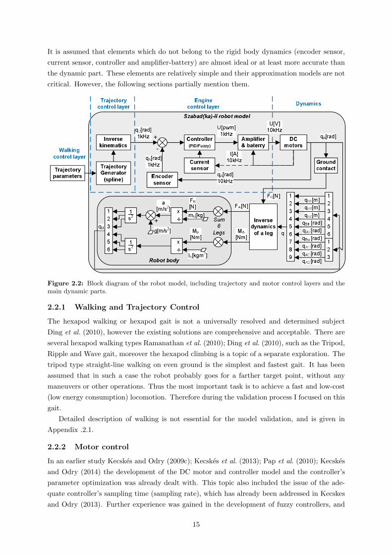
It is assumed that elements which do not belong to the rigid body dynamics (encoder sensor,

current sensor, controller and amplifier-battery) are almost ideal or at least more accurate than

the dynamic part. These elements are relatively simple and their approximation models are not

critical. However, the following sections partially mention them.

Figure 2.2: Block diagram of the robot model, including trajectory and motor control layers and themain dynamic parts.

2.2.1 Walking and Trajectory Control

The hexapod walking or hexapod gait is not a universally resolved and determined subject

Ding et al. (2010), however the existing solutions are comprehensive and acceptable. There are

several hexapod walking types Ramanathan et al. (2010); Ding et al. (2010), such as the Tripod,

Ripple and Wave gait, moreover the hexapod climbing is a topic of a separate exploration. The

tripod type straight-line walking on even ground is the simplest and fastest gait. It has been

assumed that in such a case the robot probably goes for a farther target point, without any

maneuvers or other operations. Thus the most important task is to achieve a fast and low-cost

(low energy consumption) locomotion. Therefore during the validation process I focused on this

gait.

Detailed description of walking is not essential for the model validation, and is given in

Appendix .2.1.

2.2.2 Motor control

In an earlier study Kecskes and Odry (2009c); Kecskes et al. (2013); Pap et al. (2010); Kecskes

and Odry (2014) the development of the DC motor and controller model and the controller’s

parameter optimization was already dealt with. This topic also included the issue of the ade-

quate controller’s sampling time (sampling rate), which has already been addressed in Kecskes

and Odry (2013). Further experience was gained in the development of fuzzy controllers, and

15

their performance was always compared with the PID controller Kecskes and Odry (2009b,a,

2010). The aim of further research is to reach and implement a fuzzy controller which has more

advantages in more aspects:

• Reach better performance compared to other fuzzy or PID controllers in terms of energy

consumption and device protection, as it introduced in Kecskes and Odry (2009a).

• Have sufficiently robust behavior for various loads.

• Safe behavior in case of motor and link overload as much as possible, for example, in case

when the robot gets stuck, collides, falls, etc.

During this model validation and measurements only a simple P controller (P = 0.25) was

implemented in the real robot.

2.2.3 Inverse Dynamics

The six legs of the Szabad(ka)-II robot have identical structure, but since they are driven by

different types of motors and gearheads (see details in Table 1.1), the models of the legs differ

in their parameters. Dynamic model of one leg includes three DC motors for the three joints,

one ground contact, and one inverse dynamical system.

The robotics toolbox of Peter I. Corke Corke (2001) is a Matlab toolbox developed for mod-

eling robot manipulators on fixed stand. It was chosen as the basis of the dynamics in my model,

thus the programming of dynamic formulae was not necessary, and the Simulink implementa-

tion of the robot model was faster. However, in case of walker robots the “manipulator” – i.e.

the robot leg in my case – should be attached to a moving body, and therefore this toolbox had

to be modified. In 2009 when this modeling was started Kecskes and Odry (2009a) the higher

level Simulink’s SimMechanics toolbox was not developed yet, but from 2012 my colleague also

started modeling in SimMechanics Burkus et al. (2013) due to the better usability of its toolbox.

Robot body has six degrees of freedom, three translations (X,Y, Z) and three rotations (roll,

pitch, yaw), while the leg has three more rotational joints. It is possible to build a nine-link

robot manipulator so that the first six elements are the body’s six degrees of freedom without

the weight and volume, and the last three are the actual motor-driven legs Kecskes and Odry

(2009a). Dynamics of robot body is calculated once separately from legs’ inverse dynamics

instead of attaching the same model six times to each leg. Practically the first six DOFs of

nine-link legs represent only the body kinematics, and move the stand points of the last three

DOFs according to the motion of the robot body. If the leg of one such manipulator is

kept on the ground with force F 3×1Gi , and the inverse dynamics is calculated, then the forces

of the leg acting on the body F 3×1Ai ,M3×1

Ai can be obtained. The same is calculated for the

other five legs (”i” index in equation 2.1 refers to the leg numbering; the number in superscript

designate the vector dimensions) and summarizing all these final forces are attained, which

move the body in the six degrees of freedom F 3×1B ,M3×1

B . Knowing the body weight and inertia

the robot’s body kinematics is calculated using double integration q3×1B (it is shown in Fig. 2.2).

F 3×1B =

∑i=1..6

F 3×1Ai ,M3×1

B =∑i=1..6

M3×1Ai (2.1)

16

Furthermore, by using inverse dynamics the torques of the three leg-joints can be attained, which

are feedbacked to the motor-gearheads M3×1Li . All motors are driven by a voltage controller U3×1

i

to make the joints q3×1A move according to the required values defined by the walking controls

q3×6D . Srobot parameter structure of the robot manipulator consists of a series of Links (object

defined by robotics toolbox), in the current case j ∈ 1, . . . , 9.In Appendix .2.2 Table 2 lists the main elements of the Link structure, and Table 3 shows

the parameters of the right front leg (Leg1) required by the robot object in robotics toolbox

Corke (2001). From these parameters one matrix is created and from this matrix one serial-link

object of the robot manipulator can be simply constructed. This object will be the argument

for all other functions used in this toolbox which are called from Simulink at forward kinematic

and inverse dynamics.

The inverse dynamics algorithm (see inverse dynamics block in Fig. 2.2) results reactive

forces F 3×1A and torques M3×1

A from each leg as well as torques occurring in joints M3×1L of

each leg. This algorithm uses Recursive Newton-Euler (RNE) function of the Robot Toolbox

Corke (2001), as described with equation 2.2. Table 7 in Appendix .2.2 contains variables and

parameters of the inverse dynamics model.

τ = fRNE(q, q, q, FGi, Srobot) ∼= I(q)q + C(q, q)q + F (q) +G(q) (2.2)

q = [qBX , qBY , qBZ , qBφ, qBθ, qBψ, qA1, qA2, qA3] = [q6×1B , q3×1A ]

τ = [FAX , FAY , FAZ ,MAφ,MAθ,MAψ,ML1,ML2,ML3] = [F 3×1A ,M3×1

A ,M3×1L ]

2.2.4 Robot body

Modeling of the robot body is relatively simple compared to modeling of other parts; it is based

on forward dynamics, see equation 2.3 and block diagram on Fig. 2.2. Inputs are forces and

torques acting on the body F 3×1B ,M3×1

B (the overall effect of the legs); outputs are the three-

dimensional translation and the three-dimensional rotation of the body in the world coordinate

system q6×1B . These movements can be deducted from Newton’s law a = F/m and the double

integration of accelerations which gives the translation and rotation.

qBk[m] =

∫∫(aB + gk)dtdt =

∫∫ (FBk

(t)

mB+ gk

)dtdt (2.3)

qBk[rad] =

∫∫αBdtdt =

∫∫ (MBk

(t)

IBk

)dtdt

k ∈ X,Y, Z (k ∈ Φ,Θ,Ψ in case of qBk[rad])

Table 5 in Appendix .2.2 contains the parameters of the robot body.

2.2.5 DC Motor and Gearhead

Fig. 2.3 shows the block diagram of the DC motor and gearhead model, and is described by

equations 2.4–2.10. The general model of the DC motor is defined with equation 2.10 and is

described in detail in Krishnan (2001). The gearhead model was added to the DC motor model

17

Figure 2.3: Model of DC motor and gearhead

thus the complete simulation model of the motor-gearhead pair was obtained. The controller

with UM voltage in the motor drive layer presented in Fig. 2.1 is directly connected to this

model.

The kinematic model of the gearhead is a simple multiplication with the constant of the gear

ratio rG (see equations 2.5 and 2.6). The dynamic modeling of this gearhead, however, is not

so trivial due to the internal losses. These losses are modeled by transforming the gearhead’s

inertia JG and the gearhead’s viscous friction BG into the motor side (see equation 2.7). By

doing so these quantities can be added to the internal losses of the motor, which will be the

arguments of the mechanical part of the model.

The original datasheet does not define the BM , BG and JG parameters (only JM is given),

therefore they had to be derived. The viscous friction of the motor was obtained from the

no-load operating point (equation 2.8). The viscous friction of the gearhead was approximated

from the nominal speed ωNG, nominal torque MNG and efficiency ηNG given in the datasheet

(equation 2.9). No solution has been found for the calculation of the gearhead’s inertia based on

the parameters given in the datasheet; moreover it is impossible to measure in my laboratory.

Therefore it had to be assumed that the gearhead’s inertia equals the motor’s inertia JG ≈ JM .

This way the predicted value was not significantly exceeded, because the size and weight of the

rotor and gear are in the same order of magnitude.

[IM , qA] = fM+G(UM ,ML) (2.4)

M =ML

rG(2.5)

qA =1

rG

∫ω(t)dt (2.6)

J = JM +JGr2G, B = BM +

BGr2G

(2.7)

BM =KMI0ω0

(2.8)

BG =MBG

ωNG≈ (1− ηNG)MNG

ωNG(2.9)

18

ω(s) =KMUM (s)

s2(JL) + s(BL+ JR) + (BR+K2M )

(2.10)

+−(sL+R)M(s)

s2(JL) + s(BL+ JR) + (BR+K2M )

IM (s) =UM (s)−KMω(s)

sL+R

Table 4 in Appendix .2.2 summarizes the variables and parameters of the motor-gearhead model.

The gearhead simulation model had been theoretically validated by comparing the charac-

teristic curves of my model with the curves given in the original Faulhaber datasheet Faulhaber

(2005). Fig. 2.4 shows the characteristic curves based on my simulation, which is corresponding

to the plot in datasheet. In the simulation the speed was kept constant at 5000 rpm like in the

datasheet; a Faulhaber 2232012SR motor and a PID controller was used (information about the

gearhead and controller is not mentioned in Faulhaber (2005)).

Figure 2.4: Model characteristics of gearhead

2.2.6 Ground contact

Figure 2.5: Schematic Model of Ground ContactThe ground contact is a special and critical topic in the modeling process, because the

collision between rigid bodies is a complex problem. In order to model the realistic (non-rigid)

collision between the 3D-shaped feet and the ground, one should be deeply involved in the

materials science and non-rigid body dynamics. Generally this is not the subject and aim of

dynamic and kinematic modeling in the field of robotics, because there is not an easy solution

19

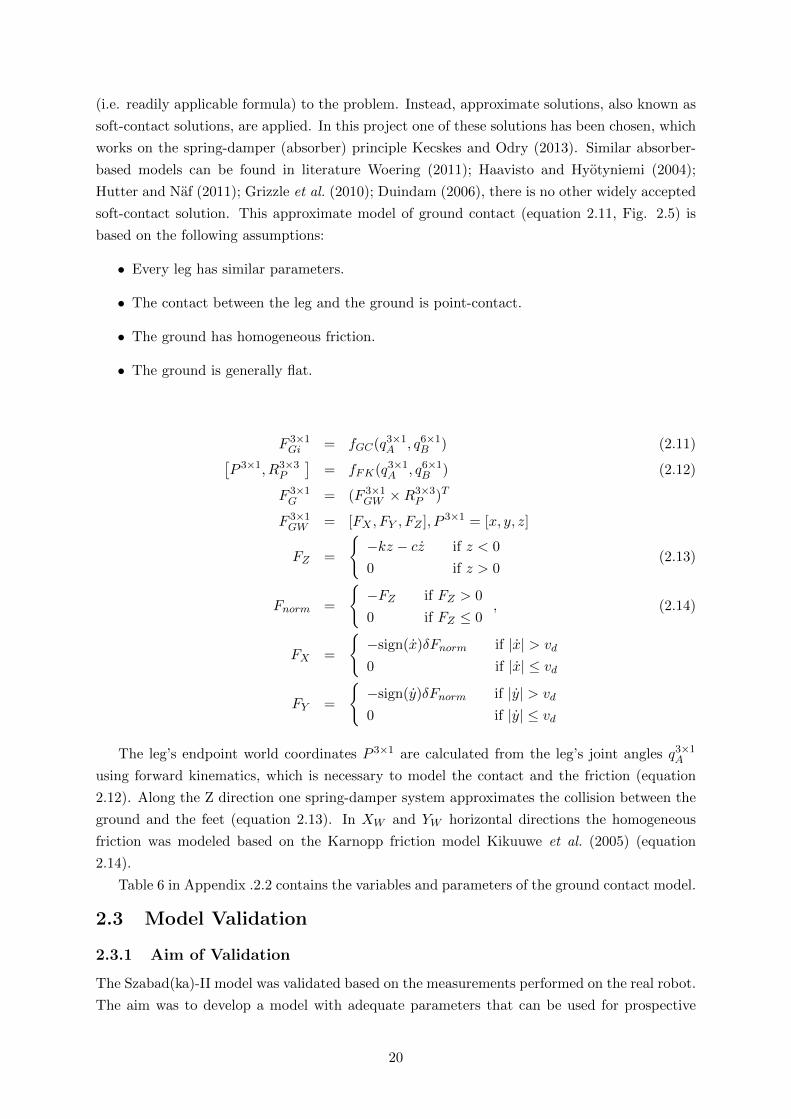
(i.e. readily applicable formula) to the problem. Instead, approximate solutions, also known as

soft-contact solutions, are applied. In this project one of these solutions has been chosen, which

works on the spring-damper (absorber) principle Kecskes and Odry (2013). Similar absorber-

based models can be found in literature Woering (2011); Haavisto and Hyotyniemi (2004);

Hutter and Naf (2011); Grizzle et al. (2010); Duindam (2006), there is no other widely accepted

soft-contact solution. This approximate model of ground contact (equation 2.11, Fig. 2.5) is

based on the following assumptions:

• Every leg has similar parameters.

• The contact between the leg and the ground is point-contact.

• The ground has homogeneous friction.

• The ground is generally flat.

F 3×1Gi = fGC(q3×1A , q6×1B ) (2.11)[

P 3×1, R3×3P

]= fFK(q3×1A , q6×1B ) (2.12)

F 3×1G = (F 3×1

GW ×R3×3P )T

F 3×1GW = [FX , FY , FZ ], P 3×1 = [x, y, z]

FZ =

−kz − cz if z < 0

0 if z > 0(2.13)

Fnorm =

−FZ if FZ > 0

0 if FZ ≤ 0, (2.14)

FX =

−sign(x)δFnorm if |x| > vd

0 if |x| ≤ vd

FY =

−sign(y)δFnorm if |y| > vd

0 if |y| ≤ vd

The leg’s endpoint world coordinates P 3×1 are calculated from the leg’s joint angles q3×1A

using forward kinematics, which is necessary to model the contact and the friction (equation

2.12). Along the Z direction one spring-damper system approximates the collision between the

ground and the feet (equation 2.13). In XW and YW horizontal directions the homogeneous

friction was modeled based on the Karnopp friction model Kikuuwe et al. (2005) (equation

2.14).

Table 6 in Appendix .2.2 contains the variables and parameters of the ground contact model.

2.3 Model Validation

2.3.1 Aim of Validation

The Szabad(ka)-II model was validated based on the measurements performed on the real robot.

The aim was to develop a model with adequate parameters that can be used for prospective

20

research (developing and optimizing the walking algorithm like in Kecskes et al. (2013) and Pap

et al. (2010)). After implementing such a walking algorithm on the real robot it would show

the same behavior, at least within an acceptable confidence interval.

As the outcome of the validation process it is expected that the difference between the results

of the current model and the measurements are within a tolerances. Therefore these tolerances

must be defined primarily from the aspects of walking and control.

2.3.2 Validation progress

Fig. 2.6 shows the validation procedure, where the gray blocks are measurement processes

performed on the robot, the light gray blocks illustrate the simulation processes, and the white

blocks show the validation processes. Basically during validation the measurements on the robot

Figure 2.6: Flow diagram of model validation progress

and the simulation results were compared. First the recorded signals were synchronized, and

then statistical methods were used to quantify the differences. If the difference between these

results was more than the specified tolerances, further studies were conducted to find the reason

of the significant deviation. The reasons of the differences are likely to be the imperfections of

the model because it is only an approximated model. Other reasons might be errors occurred in

the analog or digital measurement processes. The scope of this validation also includes exploring

and correcting these errors, illustrated by the feedback branches in Fig. 2.6. Before comparing

the signals, two prior tasks have to be completed:

• Implementing the measurement modules and communication units on the real robot to

provide the dynamic measurements taken on the robot towards the PC while walking.

21

• Measuring some specific parameters – that were possible to measure in my laboratory –

and were required for the simulation model: weight, dimensions and inertia of robot body

and the leg parts, battery voltage, battery’s internal resistance, etc.

For determining the tolerance values the following aspects should be taken into account: 1) pur-

pose of simulation (Section 2.3.3); 2) imperfection of the model (Section 2.3.4); 3) measurement

error (Section 2.3.5). The following three subsections discuss these in detail.

2.3.3 Simulation Goal

The term “simulation” in this project refers to the calculation procedure performed with the

dynamic robot model, and the determination of the chosen input and environment parameters.

In my simulations the robot is walking on a flat ground with the same walk parameters as the

real robot during the measurements.

Once the goal of a given simulation is defined, the desired precision (tolerance) of certain

physical quantities can be determined. The simulation goals were defined for the following

phases based on my expectations:

• Validation phase – during the validation process

– Goals:

∗ point to possible problems of the real robot or measurements

∗ set guidelines for building an improved robot

∗ determine model imperfections and improve them if it is worthwhile

– Expectations:

∗ estimate non-measureable parameters and their tolerance domain

∗ reveal weaknesses in robot structure and robot mechanics

∗ reveal possible faults of the model

• Prospective phase – during the research with the simulation model

– Goals:

∗ optimize the motor controller, which should be suitable for various gait and for

variable terrain conditions; moreover protect the device in any extreme cases like

falling or collision; see previous research about drop tests in Kecskes and Odry

(2009b)

∗ optimize gait and robot leg trajectories

∗ precisely implement the motor controller and leg trajectories into the robot’s

micro-controllers

– Expectations:

∗ the three-dimensional motions of the legs and the body should be realistic with

a predefined tolerance

∗ suitable modeling of the driving elements (motors, gearheads, links, frictions,

and ground contact) and the motor control unit

22

∗ imitating real events with simulations in different cases – not only in the case of

straight walking, but, for example, in case of a collision

In conclusion it is expected from all kinematic and dynamic parts of the current model to achieve

an acceptable analogy to reality.

2.3.4 Model Imperfections

The question related to the imperfection of this model is what counts or does not count as

negligible value. For example, if the estimation of a certain parameter has 10% tolerance in the

model, the expected deviation from the simulation results should also be at most in this range.

The main reasons for the imperfection of the model could be summarized as follows:

• Mechanical reasons – in reality there is no absolute precision, symmetry and similarity,

although this is assumed in modeling.

– Size differences between legs – causing asymmetric motions and forces in reality.

– Differences in friction parameters between joints.

– Non-homogeneous mass distribution of bodies – inaccuracy of body dynamic mea-

surements calculated by the SolidWorks simulation.

– Non-ideal flatness of the ground – the walk of the robot on an ideally flat ground

is un-accomplishable with an adequate accuracy (∼ 0.1mm), since I do not have

appropriately equipped laboratory.

• Electronic reasons – these are similar to the mechanical reasons only they concern elec-

tronic elements

– Differences between motors and gearheads, and deviation from the given datasheet

values.

– Lack of modeling of encoder sensors–the real encoder sensor has some inaccuracy, a

particular resolution and some delay, which are not dealt with in the current model.

– Lack of modeling of PWM amplifier–it is not modeled either.

– Deviation of power supply parameters from data given datasheet values.

– Battery recharge level – if a battery is applied.

• Approximated modeling – The simple mathematical model of certain robot parts cannot

be described (for example see Section 2.2.6), thus stochastic elements or approximate

solutions should be introduced. However, using very complex algorithms with high com-

putational time they could be more realistically modeled Renda et al. (2014). These parts

usually have a simpler approximate substitute which was also used in the current model

(see Section 2.4.5). The parameters of such approximate models have been more correctly

estimated with the help of optimization.

– The collision of legs with the ground was approximated as point-contact, while in

reality it is a non-rigid touch and friction of three-dimensional surfaces. This simpli-

fication was used for there is no viable alternative, see Section 2.2.6.

23

– The rubber soles on the feet were approximated with absorbers (spring and damper).

– The gearlash (backlash) in the links has not been implemented in the model, because

I was interested in identifying imperfections of the robot and its dynamical model,

rather than describing in detail the transient imperfect behaviour.

• Estimated parameters – There were parameters with no available datasheet value. This

kind of error source is also examined in Renda et al. (2014). In this case calculations were

not done with values determined by any kind of estimation algorithm, but values based and

determined on human estimation and my experience. In several cases certain parameters

were set using simulation and the adequacy was checked based on the expected behaviour.

The deviation of these parameters from the real values can of course be significantly high;

therefore these parameters are often the subject of optimization. This is described in

Section 2.4.

– Internal inertia of the gearhead.

– Friction coefficients, for example, the frictions of gears in the joints, which can change

while moving.

– Gearlash estimated parameters.

• Calculation imperfection of the simulator are related to

– Calculations of the Simulink’s Fixed-Step solver with 5 kHz sample rate, discussed

in paper Kecskes and Odry (2013).

– Integral calculation and rounding errors – probably negligible when compared with

other errors.

2.3.5 Measurement error

The recordings of particular signals were performed with the robot’s data acquisition system

which in this study is referred to as “measurement”. If the difference between reality and

simulation is smaller than the measurement error, this precision counts as false precision. The

measurement error was estimated with the help of:

• Test-Retest Reliability Trochim (2006) – the difference between subsequent measurements.

The measurement of robot walking has been performed several times successively.

• Parallel-Forms Reliability Trochim (2006) – Comparison of simultaneous measurements

taken on robot parts with identical behavior. In the current study there is a difference

between the robot legs, as they are same only in theory.

• Some parameters of electronic elements – Examples: tolerance of measurement-resistors,

bit-depth of ADC, effect of temperature fluctuations, stability of power supply voltage.

• Validation of measuring electronics – This has not been performed with instruments, but it

can be deducted from the experimental results. For example, the sum of all motor currents

must be in accordance with the fluctuation of power supply. (This is accomplishable since

all currents and voltages are measured).

24

2.3.6 Quantification of validation

Table 2.2 describes all physical quantities compared during the validation process. Both robot

and simulation have been measured with Fs = 500Hz sample rate.

Signals from the Table 2.2 can be divided into three groups: digital, analog and supple-

mentary (supplementary measurement are introduced in Section 2.4.4). First the digital signals

have to be validated, and if they show significant deviations, then it is not worth analyzing

the analog signals. In order to find the possible digital errors, simulation of the digital part

should be analyzed in more detail (including the calculation of the desired angle calculated by

the inverse kinematics and control voltage set by the motor controller). This part is trivial,

unlike the analog part, because here a software (C-language program) was simulated, thus only

a program bug could cause any deviations. The error might also be in several different parts of

the measurement system.

The following subsections describe the implemented multiple comparison methods. I denote

the measurement of the robot with X, the number of samples with N , and the simulation mea-

surement with X, considered as an estimation of the real quantity X.

Table 2.2: Used Quantities (Measurement Points on Robot) for Validation

TypeSymbolDim.

Name Description

digitalqD[rad]6 × 3

Desired angles oflinks

Calculated by the inverse kinematical program which runsin the MSP430Fxxxx controllers on the IK board.

digitalUP [V ]6 × 3

Control signals ofPWM amplifier

Calculated by the control algorithm located is theMSP430Fxxxx controllers.

analogq[rad]6 × 3

Angles of linksThe velocity of the angles can be measured with theencoders mounted on the motors, and the absolute anglecan be calculated based on the integration of this velocity.

analogIM [A]6 × 3

Motor currentsThe absolute value of motor current can be measured bythe IK boards.

analogUS [V ]6 × 1

Supply voltages

The voltage of the battery is also measured by the IKboard. Every IK board measures the same voltagetherefore the differences provide information aboutmeasurement errors.

supple-mentary

qPOT [rad](6 × 3)2 × 3

Real angles of links(real-pot)

The potentiometer mounted on two legs: front right (Leg1)and middle right (Leg3)

supple-mentary

qBODY [g]3 × 1

Robot bodyacceleration

Accelerometer mounted to the center of the robot body

2.3.6.1 Timely comparison of one synchronized walking cycle

To express the deviation numerically I can calculate the Mean Squared Error (MSE) value

(equation 2.15), or the Mean Absolute Error (MAE) value (equation 2.16). MAE was used

in order to express the error in a simpler measurement unit, moreover it is used in other robot

model validation Renda et al. (2014); Kubelka et al. (2014). If MAE is to be expressed relatively

then the difference must be compared with the Absolute Mean (AM) value that is the Relative

Mean Absolute Error (RMAE), see equation 2.17.

It seems there is no generally accepted comparison function, for example, besides these

methods some others are used, like the “tip error” Renda et al. (2014), “percentage normalized

25

rms error” Lin et al. (2005).

fMSE(X, X) =

√√√√ 1

N

N∑i=1

(Xi − Xi)2 (2.15)

fMAE(X, X) =1

N

N∑i=1

|Xi − Xi| (2.16)

fRMAE(X, X) =fMAE(X, X)

fMA(X), (2.17)

fMA(X) =1

N

N∑i=1

|Xi|

2.3.6.2 Comparison of mean value of one walking cycle

Obviously it is possible to calculate the average value of the absolute signal. An absolute

expression can be calculated from two mean values, namely from the Difference of Absolute

Means (DAM), see equation 2.18, and a relative expression with the Ratio of Absolute Means

(RAM), see equation 2.19. In this study RAM has mostly been used expressed in percentage.

fDAM (X, X) = |fAM (X)− fAM (X)| (2.18)

fRAM (X) =fDAM (X, X)

fMA(X)(2.19)

2.3.6.3 Spectral comparison

When there is an analog or digital filter, the spectral expression can be the most suitable

comparison method for validating the filter effects. It has been proposed to calculate an FFT-

based spectrum to at least one or more whole walking cycles. I used this method for verifying

the model of motor current measurement, i.e. there is analog low-pass filter in the electronics

(for anti-aliasing).

2.3.6.4 Confidence interval

More measurements have been performed on the walker robot in order to observe the tolerances

and confidence intervals of the whole system (including the robot walking and measurement

system). The measurements have shown a certain deviation but the normal (Gauss) distribution

cannot proved due to the small number of samples. For illustrative purposes one kind of

confidence function was introduced and applied to the mean value of the examined variables.

It determines an interval between the minimum and maximum of all available samples (M)

(equation 2.20).

fCONF (X1, X2, . . . , XM ) =

[min

(fAM

(X1), . . . , fAM

(XM

))max

(fAM

(X1), . . . , fAM

(XM

)) ] (2.20)

26

2.3.7 Tolerance Classification Scale

As it has been mentioned earlier, the tolerance rating scale can be defined based on the aspects

described in subsections 2.3.3, 2.3.4 and 2.3.5. The values of the tolerance domains in Table 2.3

refer to the percentage expression of the fRMAE(X, X) comparison function.

Table 2.3: Numerical and Color Designation of Tolerance Categories

Tolerance domain Category Expected cause of difference

0-2% (green)tolerance of digitalmeasurements

inaccurate sample rating; different roundingerrors between platforms; inaccuratesynchronization

2-10% (yellow)tolerance of analogmeasurements

model imperfection (section 2.3.4);measurement errors (section 2.3.5)

10-30% (orange)moderate differences,acceptable under certainconditions

model imperfection (section 2.3.4);measurement errors (section 2.3.5)

30-50% (red)unacceptably bigdifferences

some important element(s) missing in themodel

50-% (purple) extra differences serious measurement or simulation errors

If the differences are in the red category, i.e. the relative mean deviation is higher than

30% then the corresponding part of the simulation is not considered to be validated. In such

cases the model is so unreliable that its simulation results probably cannot be used for further

development.

2.4 Comparison of Results and Interpretation of Differences

The validation procedure includes several comparison cycles. The feedbacks in Fig. 2.6 refer to

a cyclically repeating development that is improved with each iteration.

1. The first technically functional cycle had been named as the “Trial” case, where the

estimated parameters have been set empirically. During this cycle the serious errors were

corrected and the validation modules refined (see feedbacks in Fig. 2.6).

2. The following cycle included the optimizations cases where the optimization procedure

estimated the mentioned parameters to minimize the differences. GA was implemented

for multi-variable optimization where the fitness value was defined as the reciprocal of the

examined differences. The description of GA can be found in papers Kecskes et al. (2013)

and Pap et al. (2010).

3. In the third cycle an attempt was made to take into account more walking methods

and speeds simultaneously, in order to search for such parameters that provide equally

satisfactory result for all situations (combinations of walking methods and speeds). The

variation of speed emerges as the most important of physical effects over which to challenge

the validity of the model Lin et al. (2005).

2.4.1 The Trial Case

Table 2.4 summarizes the comparison results of the first trial case. It also evaluates and illus-

trates these results with the help of the introduced tolerance domains and corresponding colors.

27

Table 2.4: Numerical expression and color categorization of the validation results in Trial case

Type Meas. Link RAM% RMAE%

digital qD[rad]1 0.193 0.4462 0.164 0.2913 0.010 0.021

digital UP [V ]1 3.696 9.9082 20.09 22.773 2.834 10.60

analog q[rad]1 0.72 4.2532 4.417 12.583 0.168 0.266

analog IM [V ]1 22.10 55.102 15.04 42.113 28.93 41.04

analog US [V ] 0.592 1.282

Except the motor current (see red cells in Table 2.4) the deviations of all other quantities

are within the acceptable precision domain. Moreover it can be assumed that the significant

deviation of other quantities result from this deviation of the motor current. Therefore the

subject of the validation process primarily focused into the motor currents and torques.

The simulated and measured currents differ in shape and in magnitude. Fig. 2.7 shows the

average current of the links compared to the confidence interval defined by measurements. The

average current refers to the average current flow during one walk step cycle. The confidence

intervals of measurements of the forward (FW ) and backward (BW ) walker robot are separately

marked. The three parts of Fig. 2.7 illustrate the values of three links for six legs. The simulation

results at the first and third links show smaller mean values, but the analysis of time curves

suggests that the reasons are not the same. On the second links an asymmetry between the

front and rear legs can be observed.

2.4.2 Issues Related to Motor Currents of Second Links

The deviation on the second links has a different character than on the other two links; the

average currents on the six legs are the same (between simulation and reality) but a deviation

can be observed if the front and rear legs are viewed separately. The average current at the

front and rear legs in simulation are equal (symmetric), while in reality they are not: In Fig.

2.7 it can be seen that in the case of forward walking (FW ) the average current on the front

legs is smaller (∼ 0.16mA) and on the rear legs is higher (∼ 0.23mA), conversely in case of

walking backwards (BW ) it is the opposite.

In order to find out the reasons for the mentioned phenomenon the motor currents in the

second link (Link2) on the front right leg (Leg1) were compared with the motor currents on

the rear right leg (Leg5), see Fig. 2.8. The acceleration of robot body can be seen above in

walking direction XW (measured with an accelerometer). The sign of acceleration concerning

the backward walk was changed in order to make the comparison easier with the forward walk.

The acceleration curves do not differ in terms of shape which means that the robot produces

the same vibrations for both walking directions, i.e. the walk is the same regardless of the

direction. By comparing the currents the same trend can be seen as in the case of mean values

28

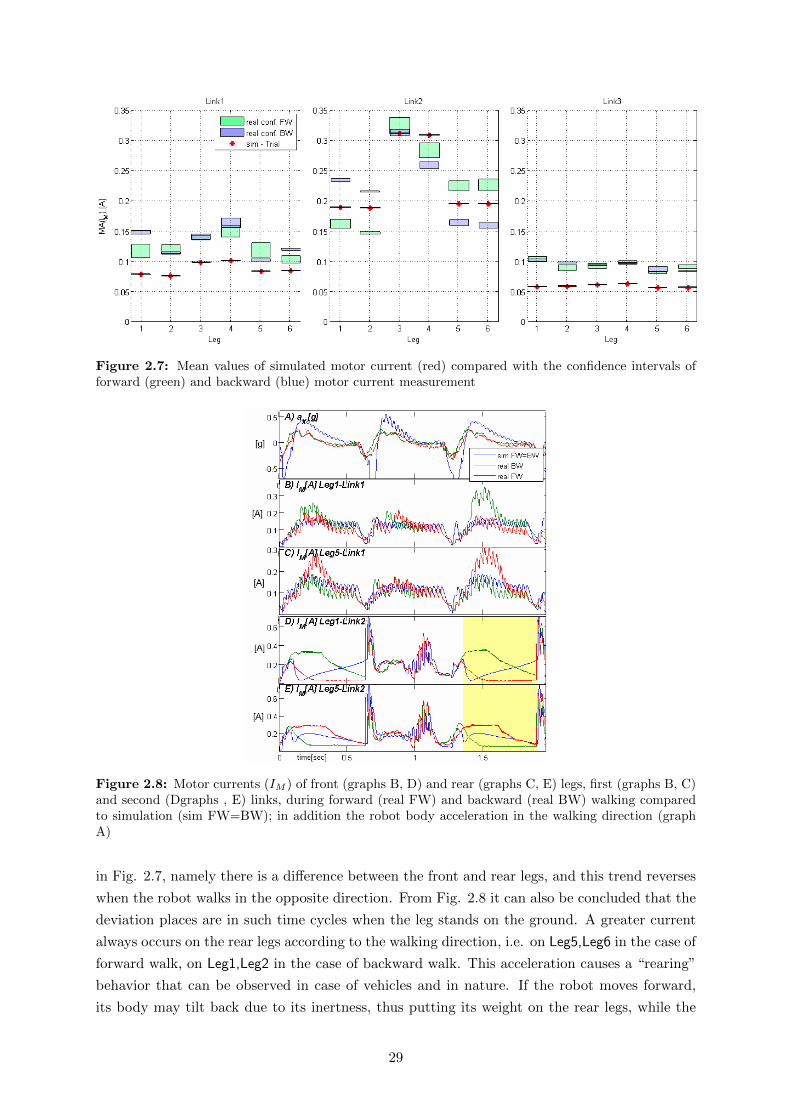
Figure 2.7: Mean values of simulated motor current (red) compared with the confidence intervals offorward (green) and backward (blue) motor current measurement

Figure 2.8: Motor currents (IM ) of front (graphs B, D) and rear (graphs C, E) legs, first (graphs B, C)and second (Dgraphs , E) links, during forward (real FW) and backward (real BW) walking comparedto simulation (sim FW=BW); in addition the robot body acceleration in the walking direction (graphA)

in Fig. 2.7, namely there is a difference between the front and rear legs, and this trend reverses

when the robot walks in the opposite direction. From Fig. 2.8 it can also be concluded that the

deviation places are in such time cycles when the leg stands on the ground. A greater current

always occurs on the rear legs according to the walking direction, i.e. on Leg5,Leg6 in the case of

forward walk, on Leg1,Leg2 in the case of backward walk. This acceleration causes a “rearing”

behavior that can be observed in case of vehicles and in nature. If the robot moves forward,

its body may tilt back due to its inertness, thus putting its weight on the rear legs, while the

29

front end practically rises. The simulated holding forces between the legs and the ground in

direction ZW illustrate this behavior shown in Fig. 2.9: the FZ continuously increases at Leg1

and decreases at Leg5 while it is constant at Leg3.

Figure 2.9: 3D projection of simulated holding forces on front (Leg1), middle (Leg3) and rear (Leg5)feet, and the real and simulated robot acceleration in walking direction (aX)

However, the question, why this asymmetric motor current phenomenon does not occur

in the simulation is still not answered. In the studied simulation the robot moved forward,

moreover, its parameters were optimized with a measurement when the robot also moved for-

ward. It can be said that this model is “prejudiced” to forward walking. In spite of this, in

the simulation the torque (or current) on the rear legs is not as big as in the real robot. The

two bottom graphs (D, E) in Fig. 2.8 (marked with yellow) show the simulation curves when

the force distribution turns at the end of the walking cycle; the front legs have greater current,

while in the measurements zero current remains and a stable strong current can be observed in

the rear-end. In the meantime the robot stops accelerating, i.e. its acceleration reduces to zero,

thus the simulation curve is more logical since the “rearing” phenomenon must also cease.

It was assumed that this phenomenon is caused by the internal stall torque in the gearheads

which for a certain time prevents the reaction forces exerted by the legs to act on the higher speed

motor side. (The motor stall torque is given for Faulhaber serial model 2232 MS = 46.8mNm,

and for the model 2342 MS = 80.0mNm Faulhaber.com (2014), but the gearhead stall torque

is not referred to.) When the forces exerted on the rear legs cease, the links do not move due to

this friction and the gearhead continues to keep the torque on the motor. On the front legs the

30

gearhead stands in a mode that does not transfer torque and when the load acts continuously it

keeps the force due to its friction and the torque is not forwarded to the motor. These holding

forces cease the moment gears start to move. This phenomenon has not been incorporated into

my model.

2.4.3 Issues Related to Motor Currents of Third Links

The motor current curves at the third links are similar in terms of shape; there are differences

only in their magnitude (see Fig 2.22). It could be supposed that the main reason for these

differences is due to the imperfect modeling of friction losses, or any other imperfections in the

other links. Therefore an attempt was made to determine the parameters not measured but

which have significant influence on the phenomenon in the third links. Practically these are the

parameters of the ground contact model: the parameters of the friction model in horizontal, and

the parameters of the spring damper model in vertical axis. In fact, these are approximation

model parts and their parameters cannot be measured, since in reality there are no matching

values. For this reason they can be estimated and validated only with the help of simulation

(see in Section 2.3.3).

GA was used to optimize the mentioned parameters. The aim was to make the motor

currents IM,l,3 at the third links more similar to the measured current IM,l,3. This was realized

with a fitness function based on the mean results of the comparative MAE function calculated

on all six currents in Link3 (equation 2.21). (MAE measurement unit is ampere.)

FIM =1

6

6∑l=1

fMAE(IM,l,3, IM,l,3) (2.21)

The original fitness value of the trial case was 39mA, and after the optimization it was reduced

to 28.8mA, while the confidence interval of the measurements was 13mA. The difference

between the mean current of a walking step (DAM) has also improved: it decreased from

28mA to 9mA. Fig. 2.10 shows these results separately of each of the six legs compared to the

measurement errors. The green blocks are the confidence intervals of the measurements, the

red blocks are the trial simulations and the blue blocks are the optimized simulation cases.

The relatively expressed fitness values are summarized for all three links in Table 2.5, which

shows that the optimization procedure does not essentially affect or improve the deviation on

the first and second links. It further supports my assumption that these optimized parameters

mostly influence the third links. This optimization case marked as Link3-Opt and compared to

Trial case.Table 2.5: RMAE Comparative Values for All Three Links

Meas. LinkRMAE%

TrialRMAE%Link3-Opt

IM [A]1 55.10 50.682 42.11 43.273 41.04 29.20

The optimization was performed several times with various parameters and parameter lim-

its, and the results were similar each time. Table 2.6 contains the trial and optimized values of

31

current parameters.

Figure 2.10: DAM, MAE, AM comparative motor current values in trial (red) and optimized (Link3-Opt) (blue) cases beside the real measurements (green); height of blocks illustrates the confidence interval

2.4.4 Issues Related to Motor Currents of First Links

The mean values (Fig. 2.7 and Fig. 2.10) do not show that the motor-current shapes of the

first links are considerably different; however, the time curves (Fig. 2.11) reveal this difference.

Fig. 2.11 shows the current time curves of the Trial simulation case and the corresponding

measurement. There are some nearly identical short periods where the difference is only in

magnitude – the reasons for this may be similar to the reasons discussed in the case of third

links. In spite of this the currents differ in certain longer periods which, for example, can be

seen between 0.6 − 1.0 second in Fig. 2.11. These deviations are higher than the acceptable

tolerance, see red cells in Table 2.4.

It became evident that robot links have a gearlash (also known as backlash), with a mag-

nitude so large that it can be observed without measurement. The gearlash exists mostly in

the first links but its cause is still to be determined. It might occur both in the gearhead and

between the bevel gears. It was assumed that the intermittent deviation of the motor currents

in Link1 could be traced back to the gearlash, thus this possibility was further analyzed.

It is important to point out that this gearlash does not participate in the control cycle, since

the encoder, mounted onto the motor, measures the angle before the gearlash-phenomenon.

Therefore the angle signals measured with the encoder (signals of link position, named “real-

enc”) contain only the reaction of the gearlash from which it is impossible to properly derive

what is happening on the opposite side of the gears. This is the reason why the angle of the

first link was also measured with a potentiometer named as “real-pot” and marked as qPOT .

32

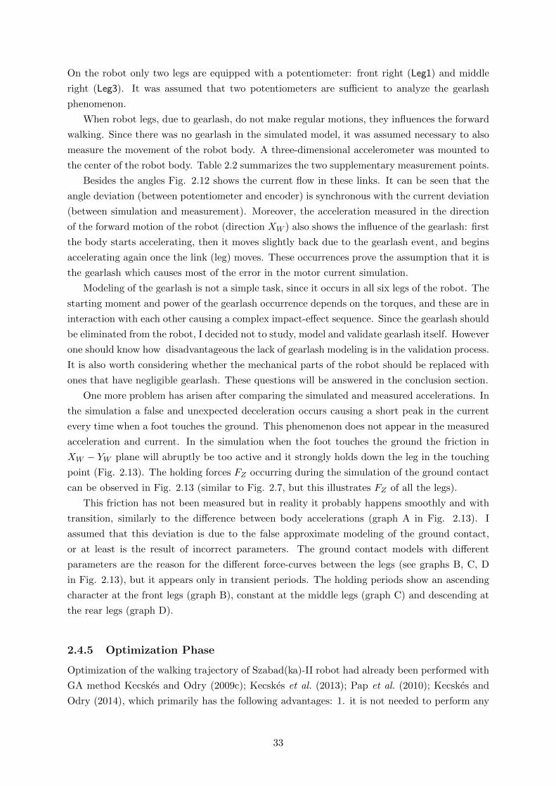
On the robot only two legs are equipped with a potentiometer: front right (Leg1) and middle

right (Leg3). It was assumed that two potentiometers are sufficient to analyze the gearlash

phenomenon.

When robot legs, due to gearlash, do not make regular motions, they influences the forward

walking. Since there was no gearlash in the simulated model, it was assumed necessary to also

measure the movement of the robot body. A three-dimensional accelerometer was mounted to

the center of the robot body. Table 2.2 summarizes the two supplementary measurement points.

Besides the angles Fig. 2.12 shows the current flow in these links. It can be seen that the

angle deviation (between potentiometer and encoder) is synchronous with the current deviation

(between simulation and measurement). Moreover, the acceleration measured in the direction

of the forward motion of the robot (direction XW ) also shows the influence of the gearlash: first

the body starts accelerating, then it moves slightly back due to the gearlash event, and begins

accelerating again once the link (leg) moves. These occurrences prove the assumption that it is

the gearlash which causes most of the error in the motor current simulation.

Modeling of the gearlash is not a simple task, since it occurs in all six legs of the robot. The

starting moment and power of the gearlash occurrence depends on the torques, and these are in

interaction with each other causing a complex impact-effect sequence. Since the gearlash should

be eliminated from the robot, I decided not to study, model and validate gearlash itself. However

one should know how disadvantageous the lack of gearlash modeling is in the validation process.

It is also worth considering whether the mechanical parts of the robot should be replaced with

ones that have negligible gearlash. These questions will be answered in the conclusion section.

One more problem has arisen after comparing the simulated and measured accelerations. In

the simulation a false and unexpected deceleration occurs causing a short peak in the current

every time when a foot touches the ground. This phenomenon does not appear in the measured

acceleration and current. In the simulation when the foot touches the ground the friction in

XW − YW plane will abruptly be too active and it strongly holds down the leg in the touching

point (Fig. 2.13). The holding forces FZ occurring during the simulation of the ground contact

can be observed in Fig. 2.13 (similar to Fig. 2.7, but this illustrates FZ of all the legs).

This friction has not been measured but in reality it probably happens smoothly and with

transition, similarly to the difference between body accelerations (graph A in Fig. 2.13). I

assumed that this deviation is due to the false approximate modeling of the ground contact,

or at least is the result of incorrect parameters. The ground contact models with different

parameters are the reason for the different force-curves between the legs (see graphs B, C, D

in Fig. 2.13), but it appears only in transient periods. The holding periods show an ascending

character at the front legs (graph B), constant at the middle legs (graph C) and descending at

the rear legs (graph D).

2.4.5 Optimization Phase

Optimization of the walking trajectory of Szabad(ka)-II robot had already been performed with

GA method Kecskes and Odry (2009c); Kecskes et al. (2013); Pap et al. (2010); Kecskes and

Odry (2014), which primarily has the following advantages: 1. it is not needed to perform any

33

Table 2.6: Optimized (Link3−Opt) Parameter Values

Parameter Unit Trial value Optimized valueLeg1 Leg2 Leg3 Leg4 Leg5 Leg6 Mean

Gearhead Efficiency – Link3 % 90 37 42 35 40 43 34 38.5Spring constant kN/m 10 1.07 3.64 6.9 4.8 4.98 6.8 4.7Damper constant kNs/m 1 1.0 1.51 1.95 1.49 0.5 1.71 1.21Velocity threshold of friction m/s 0.005 0.0002Velocity of linear friction m/s 0.05 0.08Friction constant N/N 1 1.06

Figure 2.11: Simulated (Trial) and measured motor current IM of first links, left side, with wS = 20speed

mathematical calculation on the target model, only to run the simulation, 2. the time-consuming

calculation can be easily sped up using parallelized computing. In optimization process of the

walking parameters the main issue was to determine the fitness function, i.e. what counts as

optimal walking – dealt with in the above mentioned previous researches. In the current case

however, where the attempt was to estimate the parameters of the approximate model parts,

the emphasis was primarily put on the evaluation of the results and the measurement of their

reliability (using equation 2.21 as the fitness function).

Generally a multi-parameter optimization is required where M is the number of parameters,

and such a parameter combination (a gene in M dimension space) is to be found where the

specified fitness function gives the best value. Parameter values gained by running the GA

optimization cannot be interpreted as exact optimal values, since it can be seen that the opti-

mization process provides similar results for several parameter combinations (within a certain

interval). This means that the parameters do not converge towards the optimum value with

equal speed, when the fitness value is increased to the optimum. When the convergence rate

is small (or this interval is relatively wide), the obtained optimum cannot be considered as

reliable, or this parameter does not significantly play a role in the fitness function. Estimation

and analysis of this convergence rate (CR) was described in my previous paper Kecskes et al.

(2013), where it was expressed in a simple equation (see equation (28) in Kecskes et al. (2013)).

34

Figure 2.12: Comparison of potentiometer-measured angle (real-pot) with simulated (sim) and encoder-measured angle (real-enc), as well as motor currents and robot body acceleration in walking direction(aX)

Figure 2.13: A) the peak-like waves cause the false deceleration in the simulated walking (aXsim)compared with real measurement (aXreal); simulated holding forces at ground contact (FZ): B) frontlegs, C) middle legs, D) rear legs;

Fig. 2.14 illustrates an example of CR values (the internal resistance of battery parameter

Rn battery, [Ω]).

An optimization was performed where the included parameters do not belong only to the

third links (like in the case described Section 2.4.3) but include all other parameters to be esti-

35

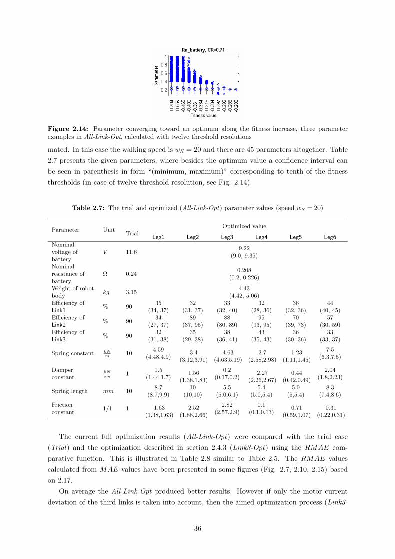
Figure 2.14: Parameter converging toward an optimum along the fitness increase, three parameterexamples in All-Link-Opt, calculated with twelve threshold resolutions

mated. In this case the walking speed is wS = 20 and there are 45 parameters altogether. Table

2.7 presents the given parameters, where besides the optimum value a confidence interval can

be seen in parenthesis in form “(minimum, maximum)” corresponding to tenth of the fitness

thresholds (in case of twelve threshold resolution, see Fig. 2.14).

Table 2.7: The trial and optimized (All-Link-Opt) parameter values (speed wS = 20)

Parameter UnitTrial

Optimized value

Leg1 Leg2 Leg3 Leg4 Leg5 Leg6

Nominalvoltage ofbattery

V 11.69.22

(9.0, 9.35)

Nominalresistance ofbattery

Ω 0.240.208

(0.2, 0.226)

Weight of robotbody

kg 3.154.43

(4.42, 5.06)Efficiency ofLink1

% 9035

(34, 37)32

(31, 37)33

(32, 40)32

(28, 36)36

(32, 36)44

(40, 45)Efficiency ofLink2

% 9034

(27, 37)89

(37, 95)88

(80, 89)95

(93, 95)70

(39, 73)57

(30, 59)Efficiency ofLink3

% 9032

(31, 38)35

(29, 38)38

(36, 41)43

(35, 43)36

(30, 36)33

(33, 37)

Spring constant kNm

104.59

(4.48,4.9)3.4

(3.12,3.91)4.63

(4.63,5.19)2.7

(2.58,2.98)1.23

(1.11,1.45)

7.5(6.3,7.5)

Damperconstant

kNsm

11.5

(1.44,1.7)1.56

(1.38,1.83)

0.2(0.17,0.2)

2.27(2.26,2.67)

0.44(0.42,0.49)

2.04(1.8,2.23)

Spring length mm 108.7

(8.7,9.9)10

(10,10)5.5

(5.0,6.1)5.4

(5.0,5.4)5.0

(5,5.4)8.3

(7.4,8.6)

Frictionconstant

1/1 1 1.63(1.38,1.63)

2.52(1.88,2.66)

2.82(2.57,2.9)

0.1(0.1,0.13)

0.71(0.59,1.07)

0.31(0.22,0.31)

The current full optimization results (All-Link-Opt) were compared with the trial case

(Trial) and the optimization described in section 2.4.3 (Link3-Opt) using the RMAE com-

parative function. This is illustrated in Table 2.8 similar to Table 2.5. The RMAE values

calculated from MAE values have been presented in some figures (Fig. 2.7, 2.10, 2.15) based

on 2.17.

On average the All-Link-Opt produced better results. However if only the motor current

deviation of the third links is taken into account, then the aimed optimization process (Link3-

36

Table 2.8: Final results of the comparison of optimization cases and the trial case

Meas. LinkRMAE Trial RMAE Link3-Opt RMAE All-Link-OptFig. 2.10, Table 2.3 Fig. 2.10 Fig. 2.15

IM [A]1 55.10% 50.68% 30.03%2 42.11% 43.27% 37.35%3 41.04% 29.20% 37.51%

average 46.08% 41.05% 34.96%

Opt) gives a better approximation model. However, the model from the current optimization

(All-Link-Opt) was taken as the final one, which probably demonstrated the best approximation

during this research, at least with the given walking conditions.

Fig. 2.15 shows the difference between the trial and optimized cases broken down for each

single link, and compares them with the confidence interval of the measurements. Mean values

of the fitness results of six legs are marked with dashed lines, and it can be seen that the

optimized case (blue) came closer to the measurements (green) in almost all graphs.

Figure 2.15: DAM , MAE, AM comparisons between trial and optimized cases, walking speed wS = 20

Fig. 2.16 shows the comparison between the measurement and simulation for the sum of

all 18 motor currents. The significant differences are due to the imperfections of the model

discussed in more detail in the next section. The optimization process performed on the model

could not approximate these dynamic differences even after having found the best parameter

combinations. Dynamic differences support the fact that the deviation is caused by effects

not incorporated into the model: major contribution is from the gearlash (discussed in section

2.4.4), followed by the imperfection of ground contact model (discussed in section 2.4.2) and

the imperfection of gearhead model (discussed in section 2.4.2).

37

Figure 2.16: Sum of Motor Currents during One Walk Cycle in Trial and Optimized Case, in the topgraph the speed is wS = 20, and in the bottom the speed is wS = 12 Oscillation in motor current iscaused by the low-resolution stepped curve in desired angle.

2.4.6 Feedback to Improve the Model

In the current research phase modeling of complex gearlash is still a problem, but not insur-

mountable (like in Veres (2013)) and is left for a future research. From the validation and

measurement results I concluded that the gearlash in the first link disturbs the walking (the

other two links do not influence it so significantly, see Table 2.9). With further measurements

and modeling it could be stated that, for a new generation robot how much emphasis should

be placed to solve the following:

• How much effort should be put on the design of the joints and other elements – to what

extent does this influence the quality of walking?

• How precise should the building of particular elements be (the issue of price versus neces-

sity)?

• Is it necessary to build another type of joint or an entirely new leg?

The problem of gearlash in the process of modeling could be further clarified, but it is more likely

that the problem will be corrected mechanically i.e. the gearlash will be avoided in the new

generation robot. In this study the alternatives of the approximate model of ground contact

have not been fully examined; only its parameters were optimized. It can be expected that

after correcting other imperfections, an improved model can be developed repeating a similar

optimization procedure, for example a better model probably would not generate the earlier

mentioned false decelerations. Namely, if a measured variable (referring mostly to the motor

current) has more sources of deviation simultaneously which do not depend only on the selected

parameters, and once they are optimized, they will lead to such a false minimum point which

can result in inaccurate estimation of these parameters. This was concluded partly on the basis

38

of high difference between the calculated optimum values of several legs; moreover these results

seem quite illogical.

The imperfect gearhead model should be further examined to determine whether such a

large deviation in simulation would cause a problem during the planned walking optimization

procedure. In such a case an improved gearhead model should be implemented into the overall

dynamical model. Based on Veres (2013) there are some usable modeling solutions for this issue:

”Most of these papers offer solutions for the modeling and identification of the mechanical system

together with the backlash phenomenon [8, 9, 10, 11, 12, 13]”

2.4.7 Feedback for Building an Improved Robot

During this research, besides perfecting the model, improvement of the robot itself was one of

the most highlighted aims. The main issue in the process of Szabad(ka)-II robot improvement

is how much attention should be paid to particular joints.

In order to answer this question in more detail, an experiment was performed, imitating the

gearlash with some noise added between the angle of the gearhead and bevel gears, while the

robot was run straight. This simple stochastic test likely similar to a realistic gearlash effect,

but it was not validated. Four cases were generated: a) there was no noise; b) noise was added

only into the first links; c) noise was added only into the second links; d) noise was added

only into the third links. The fitness value (i.e. the adequacy) of robot walking was calculated

and taken as a result. Fitness evaluation was taken from Pap et al. (2010) as a starting-point.

Table 2.9 summarizes the results where the numbers were normalized to the first noiseless

case. Besides the numerical expressions the deviation is also presented with colors, significant

deviations are shown with red, orange and yellow, while the negligible values are shown in green.

Table 2.9: Fitness of robot walking deterioration in case of additional noise in links

Property DescriptionNonoise

NoiseinLink1

NoiseinLink2

NoiseinLink3

Sum Gear Torque(f1)

sum of torques occurred inlinks

1 3.28 1.66 1.41

Body Acceleration(f2)

the squared mean of 3Dacceleration of the robot body

1 1.54 0.94 1.09

Body AngularAcceleration (f3)

the squared mean of 3D angle– acceleration of the robotbody

1 2.11 2.35 1.24

Walking Energy PerMeter (f4)

electric energy of walking forone meter

1 1.46 1.06 1.05

Average Velocity(f5)

average forward velocity indirection X (taken inversely inthe fitness function)

1 1.05 1.06 0.94

Fitness Value Papet al. (2010)f = f5

f1f2f3f4

adequacy factor calculatedwith the production of theabove indicators

1 0.07 0.27 0.47

Based on Table 2.9 I concluded that the gearlash-like problems significantly deteriorate the

quality of walking in the first links, while deterioration is less pronounced in the second-, and

39

even less in the third links.

Figures Fig. 2.17 – Fig. 2.21 illustrate a proportional comparison of the motions (kinematics)

and forces (dynamics) in all the 18 links with visual layout: (3 left links + 3 right links) × 3

leg-pairs. In the central graph the colors mark the magnitude of the examined quantity from

lower (blue) to higher (red). The left sub-graph shows the average quantity for each leg-pair

(front legs: Leg1-2, middle legs: Leg3-4, rear legs: Leg5-6), while the top sub-graph summarize

the examined quantity for each link (1,2,3)

The comparison was performed from two aspects:

2.4.7.1 Intensity of the measured signal (AM–STD–PP–V AM)

Intensity of the measured signal is a mixture of characteristic values which intend to indicate the

intensity of the signal based on various aspects: the absolute mean (AM), standard deviation

(STD), peak-to-peak distance (PP ), absolute mean of derivation or speed (V AM). It compares

the product of the four mentioned metrics, see equation 2.22.

fAM−STD−PP−V AM (X) =

√fAM (X)fSTD(X)(max(X)−min(X))fAM (X) (2.22)

Fig. 2.17 illustrates that the motion intensity is the highest in the inside (first links), and is

decreasing moving outwards, while there is no significant difference between the front and rear

legs. Fig. 2.18 shows that the motor current is explicitly intensive in the middle links, and the

highest in the middle legs. Consequently this comparison can answer the questions: to what

extent is each link overloaded, and which links and their corresponding elements should be

stronger? This results could be a guideline during the design of a new generation robot Burkus

et al. (2013).

Figure 2.17: Motion intensity (angle of link) in links during walking

2.4.7.2 Difference between the real and simulated values (MAE, RMAE)

This analysis can show which link has a modeling problem and also suggest any physical prob-

lems with the robot. Simulation error (difference between the real and simulated walk) of the

motion is smaller in the middle links of the front and rear legs (Fig. 2.19). The imperfection,

i.e. the difference, in all other links is roughly the same.

Fig. 2.20 and Fig. 2.21 show that the imperfect simulation of the motor current in the

middle links is more significant, and it illustrates an asymmetry between the right and left side,

40

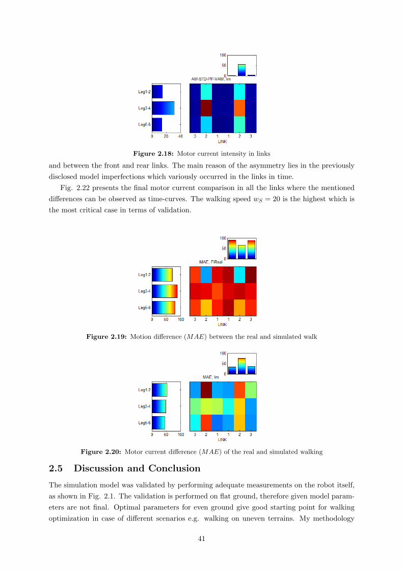
Figure 2.18: Motor current intensity in links

and between the front and rear links. The main reason of the asymmetry lies in the previously

disclosed model imperfections which variously occurred in the links in time.

Fig. 2.22 presents the final motor current comparison in all the links where the mentioned

differences can be observed as time-curves. The walking speed wS = 20 is the highest which is

the most critical case in terms of validation.

Figure 2.19: Motion difference (MAE) between the real and simulated walk

Figure 2.20: Motor current difference (MAE) of the real and simulated walking

2.5 Discussion and Conclusion

The simulation model was validated by performing adequate measurements on the robot itself,

as shown in Fig. 2.1. The validation is performed on flat ground, therefore given model param-

eters are not final. Optimal parameters for even ground give good starting point for walking

optimization in case of different scenarios e.g. walking on uneven terrains. My methodology

41

Figure 2.21: Motor current relative difference (RMAE) of the real and simulated walking

Figure 2.22: Simulated (trial case with blue, optimized case with green) and measured (red) motorcurrent comparison in all the 18 links, displayed is one walking step with speed wS = 20. The significantdifferences between simulation and measurement were discussed in sections 2.4.2 – 2.4.4

and programs can be reapplied for validating the next robot, which will walk on uneven terrain.

The validated model reached the predefined requirements in Section 2.3.3 with the reservation

for the disclosed imperfections: Some structure imperfections of the Szabad(ka)-II robot can be

identified on the basis of the validation process and the simulation results. These are followings:

1. Significant gearlash of the joint – particularly occurring in the first joints of the robot,

which influences the motor currents and harmfully affects the walking. Gearlash was

not implemented in the simulation model and this causes the majority of the differences

between the simulated and measured motor currents.

2. Imperfection of ground contact model – causing an unrealistic contact between the

42

feet and the ground during walking, i.e. it results in short false decelerations and false

peaks of the motor current.

3. Imperfection of gearhead model – neither was the gearhead’s internal non-linear

friction implemented in this model; therefore the gearhead does not behave in the same

way when affected by reactive forces as the real gearhead does. Thus in the simulation

the motor current (or torque) difference between the front and rear legs was not as large

as in reality.

The above mentioned phenomena pointed out: a) the reason of differences between the model

and the real robot; b) the places of imperfections in the model as well as in the robot. It can be

concluded that the gearlash is the most critical mechanical imperfection of the Szabad(ka)-II

robot, which deteriorates the quality of the robot motion. It can cause harmful “jumps” in the

robot motion and in the motor currents and torques. The degree of these jumps is significant

in the first joints as it was shown in sections 2.4.4 and 2.4.7. However this does not mean that

the gearlash is absent or it is completely negligible in the other joints.

The corrections of revealed imperfections of real device are essential in order to create an

improved hexapod robot. To improve the robot structure the followings should be considered:

• Design of a new robot body, including the optimal positioning of the leg mountings and a

better leg geometric design – in order to ensure equal loads of the joints, thereby to avoid

any overloads and achieve the most effective gait.

• One of the most important aims of the feet design is to minimize the unwanted acceleration

in all three dimensions during touchdown. If the feet’s spring factor is too soft it reduces

the walking quality, whereas if the spring is too hard it causes harmful acceleration in the

vertical direction.

• The 3D accelerometer was used only for validating the robot body kinematics till now.

Using the accelerometer’s signal for walking control is also an interesting challenge, which

could improve the walking quality and could be used for the protection of the robot

body. The next robot will be equipped with ground contact sensors. However, I consider

inspecting whether the data received from the single accelerometer can in certain gait

cases or completely replace the 6 ground contact sensors while walking on uneven terrain.

The presented validation procedure revealed that Szabad(ka)-II robot with some structural

improvements could be a more applicable device having higher motion quality and smaller

energy consumption. Finally, the developed simulation model will become useful for further

robot improvement because the robot structure and the drive-control can be faster and cheaper

explored with the model than with the real robot. To my knowledge there were no previous

detailed analyses of hexapod robot’s dynamic model development and validation.

The goal and usage of the Szabad(ka)-II robot simulation model is not a novelty, since

simulations of other hexapod robots – listed in Table 1.1 – were also developed in order to

improve the real robots. These simulations are used to: design the structure, define materials,

improve gait algorithms, trajectories, and motion controllers. In spite of this in the literature I

43

did not find another complete dynamic simulation model with such a detailed specification of

the model and validation as in my case. The Simulink model of Szabad(ka)-II includes:

• The model of the digital controller with a simple walking algorithm

• The realistic model of the DC motors and gearheads

• The 3D kinematics and dynamics of the 18 DOF robot

• The model of the ground contact for even ground

Some novelties were presented in this solution of model validation. These or similar methods

which cannot be found in any other hexapod simulations with a realized robot are:

• Kinematical and dynamical (time-curve) characteristics and variables of digital controllers

were compared at the same time.

• The differences of measured and simulated curves were quantified with various statistical

aspects, and qualification categories were introduced for classification of these compar-

isons.

• The unknown model parameters were estimated with a GA optimization to improve the

dynamical model. In the most extreme case 45 parameters were tuned altogether.

• Beside the model imperfections I was able to point out the imperfections of the real robot

as the conclusion of the measurement and validation procedure.

2.6 Theses Summary

2.6.1 Thesis 1

Basic conditions for validating a dynamic model of a walker robot:

• The purpose of the validated model should be determined and, according

to this, the precision requirement of the measurement variables should be

defined.

• The expected maximum precision of the dynamic model should be estimated.

The model error can not be greater than the error of the measuring system

therefore, first it should be estimated using repeated measurements and de-

viation or confidence interval calculation.

• The same control algorithm or control program must be run in the simulation

model and embedded into the robot.

• Measureable parameters must be measured 1 for the operation of the model

and the others can be estimated by model fitting optimization. It is advisable

to use heuristic optimization methods to search the global optimum of the

1relative to the capabilities of the given laboratory

44

fitting since the behavior of the walker robot is non-linear and not continuous

(primarily due to ground contact) therefore, it is non-differentiable and there

are many are unknown variables 2.

• The measurements shall be performed with the measurement units mounted

on the robot while the robot is moving or walking. The recorded signals shall

first be synchronized with the simulation results with the difference quantified

in accordance with the measurement unit of the tolerances.

• If a variable shows higher deviation that the tolerance the reason for the

deviation should be explained and, if possible, corrected. If the model is only

approximate it is expected that model imperfection is the main reason, but

it is also possible that there is a analog or digital error in the measurement

process. Therefore, the source of errors should be explored. The multi-cycle

improvement of the system belongs to the scope of validation.

This block diagram illustrates the proposed procedure on Fig. 2.6).

In the case of Szabad(ka)-II walker robot the goal was the optimization of the movement,

therefore the parameters of the walking movement and the drive controller of the joints have

been validated. These are: joint angles, controller voltage, motor currents, power voltage and

robot body acceleration. The Szabad(ka)-II robot shows 1-5% tolerance to the joint angles and

voltages, while the motor current and body acceleration shows a higher 25% relative deviation.

The statistical metric used for the Szabad(ka)-II: RMAE (relative mean absolute error).

Comparison to other research results

The tolerance definition during the SPDM robot validation was primarily built around the

purpose of the simulation and validation as well as previous simulation results (Ma et al.,

2004). My solution is different in that I have also taken into account the measurement errors

and the known imperfections of the model.

In the case of Szabad(ka)-II robot, I estimated a total of 45 model parameters using the PSO

search method. Similarly , 21 parameters of a fuzzy controller of another mobile robot is

optimized simultaneously (Odry et al., 2016). The PSO search algorithm was used by others

for fitting of a complex model such as dynamic robot model fitting (Jahandideh and Namvar,

2012). This method was also studied in theory for the robust fitting of complex nonlinear

dynamic systems (Majhi and Panda, 2011).

2.6.2 Thesis 2

In case of dynamic modeling of a walker robots the main reasons for the model’s

errors are: a) gearlash in the joints if it is not modeled, b) ground contact approx-

imation model - causing an unrealistic contact between the feet and the ground

during walking simulation thus, it results in false deceleration in the direction of

the walking and false peaks in the motor current, and c) approximation model of

gearhead, which does not include the internal nonlinear friction.

2The simplest ground contact can be approximated with a one-dimensional spring damper system having twounknowns. In addition to many feet and other unknown parameters, there are many unknown parameters andlarge search space.

45

In the case of Szabad(ka)-II walker robot the gearlash was measured by another sensor, an

external potentiometer, because the backlash occurs after the encoders were mounted on motors.

Since the controller does not receive confirmation of backlash this phenomenon damages to the

driving quality. I did not model the internal non-linear friction of the gearhead therefore, the

simulation does not work the same way when affected by reactive forces as the real gearhead

does. Thus, in the simulation, the motor current (or torque) difference between the front and

rear legs was not as big as in reality.

Comparison to other research results

Such spring-damper-based approximation models are used widely in robot modeling. In fact,

there is no other accepted methods for ground contact: (Woering, 2011; Hutter and Naf, 2011;

Grizzle et al., 2010; Duindam, 2006). Modeling of the gearlash in the joints is rare in robotics

because it is negligible in the most robots due to the partiularities of the mechanical structures.

More realistic dynamic modeling of the gearhead is a specific area, which constitutes a potential

field of further research.

46

3 Optimization Methods for Trajectory and Motor

Controller

3.1 Introduction

This chapter deals with two issues:

• Choose a relatively quick optimization method for a non-differentiable and highly non-

linear multi-variable problem, such as the most problem related to the Szabad(ka)-II robot.

Section 3.2 briefly presents the benchmarking of the optimization methods applied on dif-

ferent test functions. Multi-variable test functions have been selected for the benchmark,

which have similar characters as in the case of the walking simulation of the Szabad(ka)-II

robot (non-linear, discontinuous, integer, etc. ). The best optimizer method is chosen for

the current robot optimization problems.

• Describes the optimization procedure of hexapod walking with the help of the simulation

model: achieve an optimal trajectory curve and an effective motor controller that can be

a preliminary solution before the embedded version. The goal was to obtain a procedure

that can be generally applied for the tuning of fuzzy-based controllers if the simulation

model is available. (The implementable solution was not the focus, it is described in

chapter 4 and 5.) Section 3.3 describe how the design variables are defined of a Fuzzy-PI

motor controller.

The improvement of the robots walking on rough terrain is still in progress, including the

designing of new legs containing ground contact sensors. In the current research phase a rel-

atively simple case - the straight-line tripod walking on flat ground - was available to develop

the optimization of the robot motion and control. In order to obtain real optimal solution an

adequate model is required – this was described in the previous chapter 2.

Controller optimization with the help of the model is important because the systems per-

formance mostly depends on the controllers efficiency Jaen-Cuellar et al. (2013) besides the

structural parameters. Numerous research studies have defined the necessity and role of sim-

ulation, controller optimization and fitness function, for example in the conclusion of articles

Precup et al. (2013), Nelson et al. (2009).

3.1.1 Optimization Issue

This paper further describes an effort to search for the best optimization method that can

most effectively solve the mentioned problem (the best result in terms of performed time and

achieved fitness value). The optimization speed is very important for my system, because the

simulation of one second with Szabad(ka)-II dynamic model takes four minutes in an up-to-date

PC with a i7-2600K processor (i.e., Simulink solver with 0.2ms time step, model of 18 DC mo-

tor, 18 inverse dynamics, etc.). This means one optimization process lasts for several days, and

searching for the best optimization method with adequate parameters would last several months.

47

3.1.2 Reason for Choosing Fuzzy Control

The previous research Kecskes et al. (2013) constitutes the basis of this work, which compares

two optimization methods (GA and PSO) on a robot-walking task with a PI controller. Some of

the most successful applications of fuzzy control have been highly related to conventional con-

trollers, such as proportional-integral-derivative (PID) controller Wang et al. (2009). Currently

a Fuzzy-PI controller is being introduced and both the compared controllers are being tuned up

with the selected optimization method. The literature provides several examples of the applica-

bility of the fuzzy controller, and most of these also apply the optimization for tuning up Fuzzy

parameters, for example: Precup et al. (2013), Shoorehdeli et al. (2009), Wong et al. (2007),

Pratihar et al. (2002), Wai (2003), Wong et al. (2008), Melendez and Castillo (2013), Precup

and Hellendoorn (2011). There are less paper deals with PID controller optimization, such as

Jaen-Cuellar et al. (2013). The main difference between fuzzy logic control and conventional

control is that the former is not based on a properly defined model of the system, but instead

implements the same control ”rules” that a skilled expert would operate Wang et al. (2009).

3.1.3 Fitness Function

The most suitable optimum can be obtained primarily if the quality definition is correctly

determined. The specific robot’s walking optimality is measured by a certain fitness function

(also known as cost- or objective function). In the previous research a multi-objective fitness

function was already defined and used for the same problem Kecskes et al. (2013), Pap et al.

(2010). In this dissertation finally used a multi-scenario and multi-objective fitness formulation

discussed in chapter 4.

The tripod type straight-line hexapod walking on even ground is a simpler scenario, see

Grzelczyk et al. (2017). It has been assumed that in such a case the robot moves towards a

farther target point without any manoeuvres and other operations. More energy would remain

for the other walking modes if the energy consumption was minimized for straight line walking.

Thus the most important task will be to achieve a fast and low-cost 1 locomotion. The presented

fitness function 3.1 expresses the quality measurement of these features. It aggregates the multi-

objectives resulting in a scalar global criterion F (to be maximized) based on the weighted

product method. This described the overall quality of driving of a hexapod walker robot.

Generally the goals of robot walking are Pap et al. (2010):

1. achieving the maximum speed of walking with as little electric energy as possible, similarly

to Erden (2011),

2. keeping the minimal torques on the joints and gears,

3. maintaining the currents of the motors as little discursive and spiky as possible, and

4. keeping the robots body acceleration at a minimum in all three-dimensional directions.

F =100000 · V 2

X

EWALK · FGEAR · FACC · FANGACC · (|ZLOSS |+ 0.03)(3.1)

1low energy consumption

48

Where V 2X is the average walking speed (in direction X); EWALK - electric energy is needed

for crossing unit distance; FGEAR - root mean square of the aggregated gear torques; FACC -

root mean square of acceleration of the robot’s body; FANGACC - root mean square of angular

acceleration of the robot’s body; ZLOSS - loss of height in direction Z during the walk.

In order to obtain the results in accordance with my demands, the following should be

emphasized (equation 3.1): The average velocity tag was squared in order to emphasize it as

much as the small energy consumption and the accelerations, i.e., these two aspects influence

the system oppositely. Table 3.1 presents the six objective functions that refer to the walking

quality (3.2–3.7)

Table 3.1: Multi-objective functions for walking quality evaluation of hexapod robot

Quality Objective Objective Function

Reciprocal of Average WalkingVelocity: The robot goes in the Xdirection (xB), and higher velocity isbetter (tend simulation end time)

V 2X =

1

f1=xB(tend)

tend(3.2)

Gear Torques: Smaller torques in 6legs ×3 gears are better, ML as thetorque introduced in section 2.2.5. Incase of real robot the motor currentIM can be used if the torque is notmeasured. rms – root mean squarevalue

FGEAR = f2 = rms

( ∑6leg×3links

|ML(t)|)

(3.3)

Acceleration of body: Lower bodyacceleration aB is better in all threedimensions: X,Y, Z, aB definition seein section 2.2.4

FACC = f3 = rms(√

aBX(t)2 + aBY (t)2 + aBZ(t)2)

(3.4)

Angular acceleration of body:Lower angular acceleration αB isbetter, αB definition see in section2.2.4

FANGACC = f4 = rms(√

αBΦ(t)2 + αBΘ(t)2 + αBΨ(t)2)(3.5)

Electric energy per meter: Lowerelectrical energy consumption isbetter. Electrical energy derived frommotor current IM and voltage UM

introduced in section 2.2.5

EWALK = f5 =1

xB(tend)

∫ tend

0

∑6leg×3links

|IM (t)UM (t)|dt(3.6)

Loss of body’s height: Thesignificant loss of robot body indicatea excessive soft control, where thewalker robot unable to keep ownheight, in direction Z

ZLOSS = f6 = qBZ(tend)− qBZ(t0) (3.7)

The generalized fitness function (Fg to be minimized) can be defined as follows, see Equation

3.8. This utility function aggregatesM = 6 objectives, which is expressed based on the preceding

49

functions. The original empirically-defined weights can also be seen in equation 3.8.

Fg =M∏m=1

(bm + fm)em (3.8)

b = [0, 0, 0, 0, 0, 0.03]

e = [2, 1, 1, 1, 1, 1]

3.1.4 Leg Trajectory for Straight-Line Walking

The tripod-type hexapod walking is the most appropriate for a fast and low-cost locomotion. For

this walking a three-dimensional ellipse-based trajectory curve was generated that defines the

feet’s desired cyclic movement in relation to the robot body (see Fig. 4.1). The mathematical

description of this deformed half-ellipse trajectory can be found in Kecskes and Odry (2009c).

The trajectory curve and the driving motor controllers behaviour directly influence both

the real or simulated movement. Since the change of the trajectory’s parameters will influence

the optimal values of the other parameters that is, the parameters are not independent - the

optimal parameter set should be found in the multi-dimensional space. Therefore the chosen

motor controllers and the parameters of this trajectory (see Table 3.2) have been optimized

together. The lower (min.) and upper (max.) bounds of these parameters were defined empir-

ically in most cases, with the exception of the upper bound of the fourth ”length of the step”

(TB) parameter given by the structural dimension of the robot.

Table 3.2: Trajectory parameters and its bounds

Parameter Symbol Min. Max.The cycles time duration in [sec] TTIME 0.9 1.7Length of step - stride, in [m] TB 0.1 0.18Height of walk trajectory in [m] TH 0.01 0.04Lift (A) and cycle (A+B) ration TA/(A+B) 0.45 0.75Lowpass FIR filter strength, order in [msec], (integer) TFIR 4 300

The similar trajectory optimization attempt in Erden (2011) did not optimize the motor

controller with this trajectory; this is what is different in the current research.

3.2 Selection of Optimization Methods

There are numerous multi-variable evolutionary optimization methods, and it is generally dif-

ficult to choose the best because the performance of each method is problem-dependent Rao

(2009). Based on my experience (Kecskes et al. (2013), Kecskes and Odry (2009c), Pap et al.

(2010)) and literature (Precup et al. (2013), Rao (2009), Rios and Sahinidis (2013), Erdog-

mus and Toz (2012), Pedersen (2010)) the heuristic and hybrid methods are promising for a

non-linear, multi-variable problems.

Table 3.3 lists the selected methods that are currently under test and comparison. While

selection of the best method the existence of public Matlab implementation was taken into

account in order to avoid algorithm implementation and obtain quick results:

• Genetic Algorithm (GA) can be applied to solve problems that are not well suited for

standard optimization algorithms, including problems in which the objective function is

50

discontinuous, non-differentiable, stochastic, or highly nonlinear Goldberg and Holland

(1988).

• Particle Swarm Optimization (PSO) is one of the most important swarm intelligence

paradigms Wong et al. (2008). The PSO uses a simple mechanism that mimics swarm

behaviour in bird flocking and fish schooling to guide the particles to search for globally

optimal solutions Melendez and Castillo (2013). There is no built-in PSO algorithm in

Matlab 2014a, and thus external source exploration was needed. Considering the charac-

teristics of the available implementations, GoogleCode (2014) seems to be the good choice.

It is easy to learn, has the ordinary Matlab-like syntax, and has only the necessary options.

• Pattern Search (PS) algorithm supported in Global Optimization Toolbox by Matlab

Abramson (2002).

• Gravitational Search Algorithm (GSA) is a never-heuristic optimization method,

which is constructed based on the law of gravity and the notion of mass interactions

Rashedi et al. (2009).

• Simulated Annealing (SA) models the physical process of heating a material and then

slowly lowering the temperature to decrease defects, thus minimizing the system energy

Kirkpatrick et al. (1983).

• Teaching-Learning–Based Optimization (TLBO) is a population-based, new, effi-

cient optimization method, which works on the effect of the influence of a teacher on

learners. Rao et al. (2011)

• Tabu Search (TS) is a heuristic method but is still very limited for dealing with con-

tinuous problems. The directed tabu search (DTS) is a continuous TS that also uses the

Nelder-Mead method and adaptive pattern search. Hedar and Fukushima (2006)

• GLOBAL – The new version of ”multistart clustering global optimization method” uti-

lizes the advantages offered by Matlab, and the algorithmic improvements increase the

size of the problems that can be solved reliably with it Csendes et al. (2008).

3.2.1 Test Functions

Not all the selected optimization methods with various configurations are worth running on the

simulation model of the Szabad(ka)-II robot, because it would take half a year (see Chapter

3.1.1). This led to the application of the methods benchmark on faster test functions, and

offered a kind of pre-selection of methods based on some key characteristic behaviours. The

current dynamic model of hexapod walking - in view of character - is a multi-variable, highly

nonlinear, non-smooth, and a slightly mixed integer problem, i.e., it:

• Has a minimum of seven dimensions: PI controller has seven dimensions (5 trajectory +

2 PI design variables), while the Fuzzy-PI has 17 dimensions (5 trajectories + 12 Fuzzy

design variables).

51

Table 3.3: Selected optimization methods for the benchmark on test functions

Method Symbol SourceOwn implementation of Genetic Algorithm GA-IK Kecskes (2017)Genetic Algorithm in Global Optimization Toolbox byMatlab

GA MathWorks (2014b)

Particle Swarm Optimization PSO GoogleCode (2014)Particle Swarm Optimization with Pattern Searchhybrid

PSO-PS GoogleCode (2014)

Gravitational Search Algorithm GSA Rashedi (2011)Simulated Annealing SA MathWorks (2014c)Pattern Search in Global Optimization Toolbox byMatlab

PS MathWorks (2014a)

Teachinglearningbased optimization TLBO Yarpiz (2015a)Directed Tabu Search DTS Yarpiz (2015b)Multistart clustering global optimization methodGLOBAL, with localsearch UniRandi GLuni Csendes (2004)GLOBAL with local search FminSearch GLfmin Csendes (2004)GLOBAL with local search BFGS GLbfgs Csendes (2004)

• Has non-continuous behaviour due to walking on six legs and the ground contact.

• Has no random parts.

• Contains integer parameters, e.g., the trajectory parameter TFIR is an integer type, see

Table 3.2 and Table 3.5.

The ground contact model of the six legs - a critical part of the dynamic model – has a

discontinuous character as it can be seen in formulae (2.13) and (2.14). The backlash occurrence

at the robots links and gears also has a non-smooth feature.

Therefore test functions have been selected based on the mentioned aspects in order to

ensure the testing of these characters:

• smaller (marked with D4) and larger (D7) dimensions,

• continuous (C1) and discontinuous (C0),

• with integer (I1) and without integer (I0),

• with random (R1) and without random (R0).

Both of them can be seen in formulae 3.9 and 3.10; the rest assemble from the mixing of

presented function tags. The exact optimum is known. Selected methods run as constrained

optimization, and the test function has been scaled in order to support unified side constraints

−1 ≤ x ≤ 1, except the integer parameter, which has 0 ≤ x ≤ 10 ranges. These test functions

can be downloaded from the webpage Appl-DSP.com (2011).

52

fD4C0R0I1 =

∣∣∣∣∣∣∣∣∣∣∣1 + 1

0.1round(10x1)−0.9

∣∣∣+ round(x3)−810 +

+sgn(x4 + 0.4) +

log2(|x2 + 1.3|+ 1), x2 ≥ −0.3

log2(|1.8− x2|+ 1), x2 < −0.3

∣∣∣∣∣∣∣∣ (3.9)

fD7C1R1I0 =

∣∣∣∣∣∣∣∣1 + 1

x1−0.9

∣∣∣+ (x2 + 0.5)2 +√|x3 + 0.2|+

+rand(1)√|x4 + 0.6|+ log2(|x5 + 2|+ 1) + |x6−8|

10 + x7 − 0.6

∣∣∣∣∣ (3.10)

fD7C0R0I1 =

∣∣∣∣∣∣∣∣∣∣∣

∣∣∣1 + 10.1round(10x1)−0.9

∣∣∣+√|0.1round(10x3) + 0.2|+

+(x2 + 0.5)2 +√|x4 + 0.6|+ |x6−8|

10 + sgn(x7 + 0.4)

+

log2(|x5 + 1.3|+ 1), x5 ≥ −0.3

log2(|1.8− x5|+ 1), x5 < −0.3

∣∣∣∣∣∣∣∣∣∣∣(3.11)

−1 ≤ xi ≤ 1 i = 1, 2, 3, 4, 5, 7, 0 ≤ x6 ≤ 10

min(fD4C0R1I1) = 0, min(fD7C1R1I0) = 0, min(fD7C0R0I1) = 0

The discontinuous (C0) and seven dimension (D7) functions are more interesting for the

present problem. Bearing in mind the previous facts and assumptions the D7C0R0I1 function

is the closest to this simulation system as the objective function. It is expected that the robot-

walking problem will be effectively optimized with the methods providing better results for

such a test function that has the same characteristics as the problem. This assumption was

confirmed in this study.

3.2.2 Optimization Benchmark on Test Functions

Each optimization method was run N = 100 times with various configurations on all test func-

tions. The configuration refers to some main parameters of a certain optimization method,

which was randomly selected in each case (for example, in the case of GA: generations, popu-

lation, elite count, crossover type).

Fig. 3.1 shows the results in case of four-dimension test functions, while Fig. 3.2 and Fig. 3.3

illustrate the seven dimension cases. The left-bottom corners represent the best performance,

i.e., the better fitness on the horizontal axis and the smaller number of function calls on the

vertical axis. An acceptance condition was defined, and plotted with a magenta line. Different

performance clouds can be seen in cases of various types of functions. There are more methods

reaching acceptable results for the four-dimension problem (Fig. 3.1). However, in case of seven

dimensions (D7) and discontinuous (C0) benchmark only the PSO, the PSO-PS hybrid, and

TLBO methods reach really acceptable results (Fig. 3.2 and 3.3). The following findings can

be obtained from the clouds in Fig. 3.2 and 3.3:

• The PSO, PSO-PS, and TLBO methods provide the best stable results for all the discon-

tinuous functions.

• The PSO-PS hybrid method contains the good performance of PSO and the stableness of

PS. Thus this will be the best choice for higher dimension problems, especially in the case

of D7C0R0I1 function (left-top graph in Fig. 3.3), which is most similar to the current

robot model.

53

• The GL*, PS and DTS methods reach almost the best results for the continuous functions

without random tags, but in other cases give a lower performance.

• The GA, GA-IK, GSA and SA methods do not reach acceptable results in any case. The

SA method seems to be the weakest for all types of functions.

• The GA methods reach a lower performance but keep roughly similar values for different

test functions. This reinforces the problem-independent character of GA.

• The GSA method is excellent only for the continuous problems without an integer tag,

but very weak for the others.

Figure 3.1: Optimization benchmark on functions of four dimensions (D4) and without integer (I0)

The results of this benchmark contributed and confirmed the effectiveness of the selected

PSO method as mentioned in papers Kecskes et al. (2013), Shoorehdeli et al. (2009), Pedersen

(2010), Wong et al. (2008). Similar benchmark efforts can be found in Rios and Sahinidis (2013)

where the PSO also reaches a very good performance level. In paper Shoorehdeli et al. (2009) a

benchmark of optimization methods (ANFIS, PSO among others) was also applied on a fuzzy

controller, not on the test functions. It also confirmed the PSO usability for tuning the fuzzy

system. The pattern search (PS) can refine the result from PSO (compare PSO and PSO-PS

clouds in Fig. 3.1, 3.2, 3.3). It runs after PSO and is initialized by the best entities of PSO.

Thus, the PSO-PS hybrid has become the best method for us.

3.3 Fuzzy-PI Controller

First of all the design of a controller is primarily defined by the fact that it should be im-

plemented into the microcontrollers of the real Szabad(ka) robot series. This means that the

54

Figure 3.2: Optimization benchmark on functions of seven dimensions (D7) and without integer (I0)

Figure 3.3: Optimization benchmark on functions of seven dimensions (D7) and with integer (I1)

memory and calculation demand of the controller should be maintained within certain bound-

aries. From another aspect only just the available measured quantities can be used as input (of

a Fuzzy controller) due to the given sensor interface.

Based on previous research Kecskes and Odry (2010), Kecskes and Odry (2012) a fuzzy

controller with some rules is enough for obtaining an improved result compared with the simple

PID controller. One of the key things is the fact that fuzzy can include more inputs, while the

PID has only one (the error of control variable). In case of robot link control it is the angle error,

55

i.e., the difference between the desired and measured angle. Besides this the absolute value of

the motor current was put into the fuzzy inputs; it was possible since the electronics on the

Szabad(ka)-II measures this. A similar solution was found in Wang et al. (2009), however the

authors do not explain the role of this current feedback. In addition, if required, the derivative

of angle error and the error of angle velocity could be used as input or the measured angle value

might also be applied in case the controlling behaviour is different in a certain angle section.

3.3.1 Fuzzy inputs and outputs

The block diagram in Fig. 3.4 shows the designed Fuzzy-PI controlling cycle with the inputs

and outputs. The three selected inputs are: error angle AERR, error velocity VERR, and motor

current IMA, while the two outputs are: proportional tag of voltage FzzP , and integrative

tag of voltage FzzI. A controller system with the same parameters and conditions should be

provided for each 18 DC motor of the robot. This controller has been implemented only on the

dynamic model of Szabad(ka)-II robot, when it was tested and optimized.

Figure 3.4: Fuzzy-PI motor control loop in the dynamic model of Szabad(ka)-II robot

3.3.2 Membership Functions and Rules

Fig. 3.5 presents the necessary membership functions (MFs) and the eight rules defined by the

authors, which mostly determine the controlling character:

• The first rule refers to cases when there is no error angle and the outputs come near to

zero.

• The second rule ensures that if the velocity error is small then the integration output

tends toward zero.

• The third and fourth rules ensure the output activity in order to decrease the control

(angle) error.

• The fifth and sixth rules have an opposite influence to the third and fourth rules, but only

when the motor current is high. These rules ensure a softer feature of controlling when

the currents or torques are great, and thus can protect against electrical and mechanical

overload.

56

• The seventh and eighth rules reinforce the integrative output activity for decreasing the

velocity error when the motor current is smaller.

The logic of these rules has been reinforced by earlier research Kecskes and Odry (2010), but

on the other hand the optimization process should select the necessary or dominant rules by

tuning up its weights.

Fig. 3.6 illustrates the output surfaces of the built Fuzzy-PI controller, where the aggregated

effects of the previously described rules can be observed.

Figure 3.5: Rules of Fuzzy-PI controller: first input column is the error angle, second input column isthe absolute motor current, third column is the error, first output column is the proportional tag, andsecond output column is the integrative tag.

3.3.3 Selecting Fuzzy-PI Parameters for Optimization

The number of fuzzy controller parameters depends on the number of all MFs and rules. If it

is assumed that the defined rules are suitable, then only the weight of them count as design

variables. Furthermore there is no need to count separate parameter values for the symmetric

MFs and rules. According to this the current Fuzzy-PI controller has 37 parameters in all:

• 5 method type parameters: AndMethod,OrMethod, ImpMethod,AggMethod,DefuzzMethod

• 9 MFs x 3 parameters (2 scale values+ 1 function type value (trimf or gaussmf))

• weight of 5 rules (8 rules 3 symmetry)

Despite this the parameters of MFs have been reduced by the following method: only the

range values of inputs and outputs have been changed, thus the internal MFs do not change

relative to each other. For the modification of the range values it is also necessary to convert

the parameters of the Fuzzy membership functions, for which the Fuzzy Toolboxs strtchmf

function can be applied. Additionally the MF types have been selected for optimization. The

Matlabs built-in Fuzzy Toolbox supports more MF types; however, the converting of one MF

type into a second type is not a trivial task if the character is to remain. The Fuzzy Toolboxs

mf2mf function also cannot properly convert the MFs in all cases. From the original triangle MF

(trimf) the gauss MF (gaussmf) can be converted in the easiest way, which is why only these

57

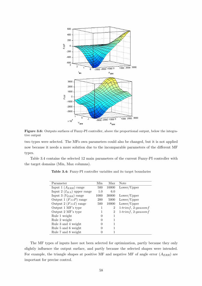
Figure 3.6: Outputs surfaces of Fuzzy-PI controller, above the proportional output, below the integra-tive output

two types were selected. The MFs own parameters could also be changed, but it is not applied

now because it needs a more solution due to the incomparable parameters of the different MF

types.

Table 3.4 contains the selected 12 main parameters of the current Fuzzy-PI controller with

the target domains (Min, Max columns).

Table 3.4: Fuzzy-PI controller variables and its target boundaries

Parameter Min Max NoteInput 1 (AERR) range 500 10000 Lower/UpperInput 2 (IMA) upper range 1.0 6.0Input 3 (VERR) range 1000 30000 Lower/UpperOutput 1 (FzzP ) range 200 5000 Lower/UpperOutput 2 (FzzI) range 500 10000 Lower/UpperOutput 1 MF’s type 1 2 1-trimf , 2-gaussmfOutput 2 MF’s type 1 2 1-trimf , 2-gaussmfRule 1 weight 0 1Rule 2 weight 0 1Rule 3 and 4 weight 0 1Rule 5 and 6 weight 0 1Rule 7 and 8 weight 0 1

The MF types of inputs have not been selected for optimization, partly because they only

slightly influence the output surface, and partly because the selected shapes were intended.

For example, the triangle shapes at positive MF and negative MF of angle error (AERR) are

important for precise control.

58

3.4 Results and Comparison

3.4.1 Optimization Results

The results of optimization can be seen in Table 3.5 for both controller types (PI and Fuzzy-

PI), and for two optimizers, PSO-PS and PSO methods. The PSO-specific configuration were:

the number of generation was selected to NG = 70, the population size was NP = 40, the

inertia weight w = 0.9, the cognitive attraction c1 = 0.5, and the social attraction c2 = 1.5.

These configuration parameters were selected partly from the literature Kecskes et al. (2013),

Shoorehdeli et al. (2009), Erdogmus and Toz (2012), Rao (2009), Pedersen (2010), Wong et al.

(2008), partly from own experience.

Table 3.6 comprises the detailed partial (multi-objectives before aggregation) results of the

fitness evaluation (3.1). However, the Fuzzy-PI-PSO method seems to be the best one if only

the lowest energy consumption and the fastest movement is considered. But the lower accelera-

tions and stability are also important for the quality, and that is why my fitness function (3.1)

takes into account all of these properties. In this respect the Fuzzy-PI by PSO-PS has the best

fitness value (without any significant differences).

Table 3.5: Optimized design variables: trajectory and controllers in Szabad(ka)-II robot model

ParameterFzz-PI byPSO-PS

Fzz-PI byPSO

PI byPSO-PS

PI by PSO

Trajectory

The cycles time duration 1.740 1.733 1.808 1.696Length of step (stride) 0.163 0.161 0.168 0.142Height of walk trajectory 0.0364 0.0329 0.0397 0.0366Lift (A) and cycle (A+B)ratio

0.564 0.544 0.574 0.577

Lowpass FIR filterstrength

12 33 93 9

PIProportional 0.454 0.340Integral 0.147 0.534

Fuzzy-PI

Input 1 range 5126 6369Input 2 upper range 4.4 1.465Input 3 range 11682 12103Output 1 range 2227 2620Output 2 range 2176 6362Output 1 MFs type 2 2Output 2 MFs type 1 2Rule 1 weight 0.066 0.234Rule 2 weight 0.996 0.281Rule 3, 4 weight 0.215 0.496Rule 5, 6 weight 0.385 0.258Rule 7, 8 weight 0.783 0.502

3.4.2 PI and Fuzzy-PI Controllers Simulation Comparison

Fig. 3.7 shows the time diagram of the robot movement (BX), velocity (BV X) acceleration

(BAMag), and the summarized motor currents (ISUM ) for five optimized cases:

• Fuzzy-PI controller optimized with PSO-PS method (red) - the best Fuzzy solution, high

fitness obtained by smaller energy consumption and smaller acceleration, see Table 3.6.

59

Table 3.6: Fitness values in cases of optimized PI and Fuzzy-PI system.

ObjectivesFzz-PI byPSO-PS

Fzz-PI byPSO

PI byPSO-PS

PI by PSO

Gear torques 8.71 9.09 8.82 9.12Body acceleration 1.77 1.89 1.77 1.80Body angular acceleration 16.09 17.09 16.39 17.2Energy per meter 41.96 41.05 42.55 42.5Loss of height -3.8e-3 -5.5e-3 -7.7e-3 -7.3e-3Mean velocity 0.156 0.163 0.152 0.152

Fitness value (higher isbetter)

6.887 6.209 5.644 5.171

Number of function calls 3872 1442 1776 645

• Fuzzy-PI controller optimized with PSO method (yellow) - the Fuzzy reached a little faster

movement than the PI besides a roughly same power consumption and body acceleration.

This was the main reason for the higher fitness value.

• PI controller optimized with PSO-PS method (blue) the best PI solution, the details can

be seen in Table 3.6.

• PI controller optimized with PSO method (green) an interesting trajectory can be ob-

served, very similar to the best Fuzzy-PI solution

• PI controller optimized with GA previously in Pap et al. (2010) (grey) it is important

to present the mentioned typical hexapod gait problem, i.e., the significant fluctuation of

velocity.

Based on the comparison of these four optimized cases and the other results obtained during

the development it can be concluded that some solutions reach the high fitness value by higher

speed, while others reach this value by smaller energy and acceleration. In spite of the difference

between the presented four cases, both control methods in all given solutions generate high

quality walking: the fluctuation of velocity is relatively small compared to a typical inadequate

hexapod walking, illustrated with grey in Fig. 3.7, and found in Pap et al. (2010), Kecskes and

Odry (2010). Mostly the motor currents have different curves due to the fact that the fuzzy

also includes the current in the control decision.

The three-dimensional leg trajectory can be seen in Fig. 3.8, related to the five mentioned

optimized cases in Fig. 3.7. The ellipse-based desired trajectory was also plotted with a little

shift besides the simulated-regulated trajectory. The simulated-regulated angle curves of three

robot leg links illustrated on the right follow the desired angle curves calculated with inverse

kinematics. The explanation of the presented link numeration can be found in Fig. 3 in paper

Burkus et al. (2013).

3.5 Discussion and Conclusion

A new and widely usable method was created for (pre)selecting the potentially best optimization

method(s) used for a given problem. The test functions for a benchmark were created includ-

ing those mathematical characteristics that are interesting or typically describe the examined

objective function (section 3.2.1). The selection of these characteristics was the key point, since

60

Figure 3.7: Comparison of optimized walking with PI and Fuzzy-PI controllers: movement (BX) attop-left, velocity (BV X) at bottom-left, summarized motor current (ISUM ) at top-right, and magnitudeof 3D body acceleration (BAMag) at bottom-right

Figure 3.8: Leg trajectory curves of four optimized cases: the desired and simulated trajectory curves(left), simulated angles of three links (right)

certain methods provide significantly different performance levels for different test functions

with various characteristics (Section 3.2.2). It can be observed that the configuration of the

optimization method also have an influence, because the random change of these parameters

formed a cloud for each method (see coloured clouds in Figures 3.1, 3.2, 3.3). The best set of

61

these parameters can also be deducted from these benchmark results.

In the current demonstrated case the objective function is the straight-line walking quality

aspects of the Szabad(ka)-II robot with a fuzzy motor controller in virtual simulation space

using the dynamic model. The design variables of this system contain both parameters of

the trajectory and the controller. If the optimization methods were tested directly on this

simulation model, the computation would take some months due to the model’s complexity i.e.,

it is specifically computationally expensive. Contrary to benchmarking on fast test functions

this takes a much shorter time: only a few hours. Thus the optimization of the robot model

has been run only with the benchmark-selected methods. The PSO and PSO-PS methods were

selected as best for the function having similar characteristics as the robot walking system. The

PSO-PS hybrid method proves to be effective compared with the earlier optimization attempts

Kecskes et al. (2013), giving significantly better results, independent of the controller type (see

Section 3.4.1). Previously the GA optimization method was used for the same walking problem,

and the results (maximum fitness) were significantly worse F = 3.78 Kecskes et al. (2013). This

research pointed to the fact that a suitable method should be found for each optimization

problem, thus reaching the best results quickly - the global optimum with higher probability.

The well-defined quality formulation and proper fitness function – i.e. multi-objectives and

its preferences – are important according to my experience.

Besides, this research also confirmed that a well-defined fuzzy type controller is a more cus-

tomizable motor controller than a simple PI controller. A relatively simple Fuzzy-PI controller

was constructed based on previous experience (see Chapter 3 in Kecskes and Odry (2010)) in

order to implement it into the microcontrollers of the real robot without any resource prob-

lems. After the optimization procedures - run with similar conditions - the Fuzzy-PI controller

reached nearly 22% better walking quality (FFZZ = 6.88/FPI = 5.64 ∼= 1.22). Of course, the

obtained controller itself is not sufficient to drive the robot with various gaits and on various

terrains, and was not tested yet on the hardware.

The multi-scenario optimization approach is discussed in Chapter 4 while the embedded

controller in Chapter 5.

3.6 Theses Summary

By measuring the quality of the drive control, it is possible to check whether the elaborated

fuzzy-based control has better quality than other controllers (such as classic PID). For compar-

ison, these reference controllers must be built up, and then the tests should be performed with

their best possible settings. To find the best possible parameters the same optimization method

is recommended for a fair comparison. In the control of Szabad(ka)-II robot’s motors, the op-

timized Fuzzy-PI controller reached an average of 20% better global fitness than the optimized

PID controller.

(Santos et al., 1996) also compared Fuzzy-PID controllers with the traditional PID controller.

Although the PID controller was determined by a classical tuning method (Ziegler-Nichols

method) and non by a searching algorithm. Nonetheless, the most of robotics research do not

compare their fuzzy-based controller performance to a simple PID or PI, for example (Mazhari

et al., 2008), so the advantage of fuzzy logic is not expressed.

62

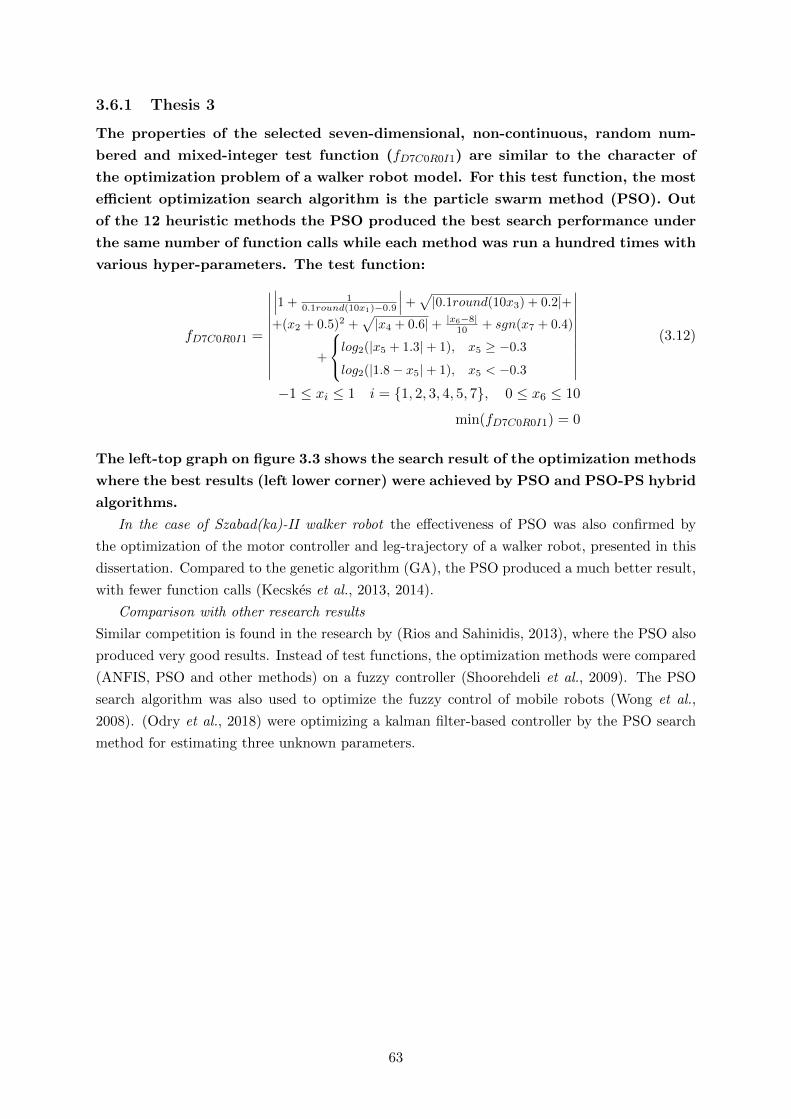
3.6.1 Thesis 3

The properties of the selected seven-dimensional, non-continuous, random num-

bered and mixed-integer test function (fD7C0R0I1) are similar to the character of

the optimization problem of a walker robot model. For this test function, the most

efficient optimization search algorithm is the particle swarm method (PSO). Out

of the 12 heuristic methods the PSO produced the best search performance under

the same number of function calls while each method was run a hundred times with

various hyper-parameters. The test function:

fD7C0R0I1 =

∣∣∣∣∣∣∣∣∣∣

∣∣∣1 + 10.1round(10x1)−0.9

∣∣∣+√|0.1round(10x3) + 0.2|+

+(x2 + 0.5)2 +√|x4 + 0.6|+ |x6−8|

10 + sgn(x7 + 0.4)

+

log2(|x5 + 1.3|+ 1), x5 ≥ −0.3

log2(|1.8− x5|+ 1), x5 < −0.3

∣∣∣∣∣∣∣∣∣∣(3.12)

−1 ≤ xi ≤ 1 i = 1, 2, 3, 4, 5, 7, 0 ≤ x6 ≤ 10

min(fD7C0R0I1) = 0

The left-top graph on figure 3.3 shows the search result of the optimization methods

where the best results (left lower corner) were achieved by PSO and PSO-PS hybrid

algorithms.

In the case of Szabad(ka)-II walker robot the effectiveness of PSO was also confirmed by

the optimization of the motor controller and leg-trajectory of a walker robot, presented in this

dissertation. Compared to the genetic algorithm (GA), the PSO produced a much better result,

with fewer function calls (Kecskes et al., 2013, 2014).

Comparison with other research results

Similar competition is found in the research by (Rios and Sahinidis, 2013), where the PSO also

produced very good results. Instead of test functions, the optimization methods were compared

(ANFIS, PSO and other methods) on a fuzzy controller (Shoorehdeli et al., 2009). The PSO

search algorithm was also used to optimize the fuzzy control of mobile robots (Wong et al.,

2008). (Odry et al., 2018) were optimizing a kalman filter-based controller by the PSO search

method for estimating three unknown parameters.

63

4 Multi-scenario Multi-objective Optimization of Fuzzy-

PI Motor Controller

4.1 Introduction

In this chapter, the optimization of the motor controller differs from previous Chapter in the

following aspects:

• Developing and optimizing a Fuzzy-PI controller which can be embedded into real robot

controllers, into one Texas Instruments MSP430F2618 microcontroller (for each leg). The

fuzzy output is calculated by a previously generated lookup table, which has a constant

number of dimensions and resolution Kecskes et al. (2015a).

• The simulation has multi-scenario properties. The multi-scenario approach is important

to develop a universally optimal and robust motor controller for the intended use of the

robot. See the details in Subsection 4.2.3.

The analyzed and optimized system is a multi-scenario multi-objective problem (MSMO). These

two properties are described in the Section 4.2. The Section 4.3 describes the Fuzzy-PI motor

controller, and the Section 4.4 summarizes the experimental results.

4.2 Multi-scenario Multi-objective Optimization

To search for the optimum solution, user needs to define and quantify the goodness of the

controller, as it was discussed in Section 3.1.3. To the best of the authors’ knowledge, there are

no specific and applicable definitions for robot control problems presents in this dissertation.

Practically, there are no definitions for the required quality aspects, nor is it clear to what

extent the aspects should be optimized. In my proposal, the goodness is divided into simpler

elements (objectives), which are established by common sense and empirical experience. Thus,

the quality description is multi-objective.

4.2.1 Multi-objective Quality Definition

Structural and control optimization issues in dynamic robotic systems are commonly multi-

objective problems, as in Kubler et al. (2005) and as described in my previous research Kecskes

and Odry (2014), Kecskes et al. (2014), Burkus et al. (2013). A multi-objective optimization

process has several objective functions, and when searching for the optimum solution, the criteria

involve finding the best fitness values while compromising between the objectives using any

preference between them Deb and Miettinen (2008).

The determination of the robot walking quality is not a trivial task. However the most

commonly seen criteria are the maximum traction and the minimum power consumption Iag-

nemma and Dubowsky (2004): ”In rough terrain, traction should be maximized. In benign

terrain, power consumption should be minimized.” In addition to the energy consumption and

maximum walking speed, the vibration and jerks that appear in dynamics are addressed. The

64

minimization of such high accelerations or rigid collisions is generally examined in robotics

Carbone (2011).

Five quality objectives were defined for the Szabad(ka)-II robot walking; see Table 4.1 (orig-

inally published in Kecskes and Odry (2014) and mentioned in Section 3.1.3).

Table 4.1: Hexapod walking objectives

Quality Goal Objective Symbol

achieve the maximum walking speed mean velocity in the X direction f5

minimize the electric energy consumptionelectric energy consumption forwalking one meter

f4

minimize the torque on the joints and gears,thus minimizing the jerks in the motorcurrent

root mean square of torquesmeasured in the 18 joints

f1

minimizing the robot’s body acceleration inall three-dimensional directions

root mean square of magnitudeof 3D body acceleration

f2

minimizing the robot’s body angularacceleration in all three-dimensionaldirections

root mean square of magnitudeof 3D body angular acceleration

f3

4.2.2 Aggregation of Multi-objectives

Some type of manual selection is required for the Pareto solution sets that result from the

multi-objective optimizer algorithms, because only one solution at a time can be implemented

in the real application. The scalar fitness values are calculated by aggregating the objectives

by a so–called utility function.

I propose a bias–weighted utility function and the production operation for the aggregation

(geometrical mean) – bias–weighted product type (BWP) utility function. This function has

a bias (bm) and exponent (em) weights for each objective. The bias weights can reduce the

strong influence of near zero values, while the exponent weights express the relative importance

between the objectives. Equation 4.1 describes this utility function resulting in the scalar fitness

value (fSC) for one simulation scenario. The X represents the design variables, M is the number

of objectives.

fSC(X) =M∏m=1

(bm + fm(X))em (4.1)

The well-defined quality formulation and proper weighting of the objectives are important

Kecskes and Odry (2014). In this study these quality definitions are used. However, the

preferences between these objectives are defined carefully and empirically. Different variations

of these preferences are presented in Section 4.4.2.

4.2.3 Multi-scenario Simulation

A driving solution is sought that provides robust and universally optimal behavior for all possible

movements or walking tasks of the walker robot. The scenario-oriented approach offers an

advantageous solution to this issue, as stated in the conclusion of Fadel et al. (2005). The

all-situation problem can thus be decomposed into several scenarios to form multiple objective

65

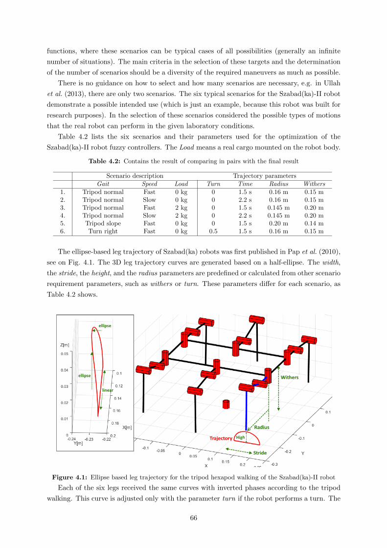
functions, where these scenarios can be typical cases of all possibilities (generally an infinite

number of situations). The main criteria in the selection of these targets and the determination

of the number of scenarios should be a diversity of the required maneuvers as much as possible.

There is no guidance on how to select and how many scenarios are necessary, e.g. in Ullah

et al. (2013), there are only two scenarios. The six typical scenarios for the Szabad(ka)-II robot

demonstrate a possible intended use (which is just an example, because this robot was built for

research purposes). In the selection of these scenarios considered the possible types of motions

that the real robot can perform in the given laboratory conditions.

Table 4.2 lists the six scenarios and their parameters used for the optimization of the

Szabad(ka)-II robot fuzzy controllers. The Load means a real cargo mounted on the robot body.

Table 4.2: Contains the result of comparing in pairs with the final result

Scenario description Trajectory parametersGait Speed Load Turn Time Radius Withers

1. Tripod normal Fast 0 kg 0 1.5 s 0.16 m 0.15 m2. Tripod normal Slow 0 kg 0 2.2 s 0.16 m 0.15 m3. Tripod normal Fast 2 kg 0 1.5 s 0.145 m 0.20 m4. Tripod normal Slow 2 kg 0 2.2 s 0.145 m 0.20 m5. Tripod slope Fast 0 kg 0 1.5 s 0.20 m 0.14 m6. Turn right Fast 0 kg 0.5 1.5 s 0.16 m 0.15 m

The ellipse-based leg trajectory of Szabad(ka) robots was first published in Pap et al. (2010),

see on Fig. 4.1. The 3D leg trajectory curves are generated based on a half-ellipse. The width,

the stride, the height, and the radius parameters are predefined or calculated from other scenario

requirement parameters, such as withers or turn. These parameters differ for each scenario, as

Table 4.2 shows.

Figure 4.1: Ellipse based leg trajectory for the tripod hexapod walking of the Szabad(ka)-II robot

Each of the six legs received the same curves with inverted phases according to the tripod

walking. This curve is adjusted only with the parameter turn if the robot performs a turn. The

66

joint trajectories are calculated from this leg trajectory using inverse kinematics, which was

described in a previous Section 2.2.

4.2.4 Aggregation of Multi-scenario

Parallel execution of these scenarios provides a multi-scenario objective function that is pri-

marily a multi-objective function. Multi-scenario problems are regularly solved by aggregating

all objectives of all scenarios into a large multi-criteria problem, which is confirmed by studies

Fadel et al. (2005), Zhu et al. (2014). The global scalar fitness values (fG) are calculated with

the geometrical mean applied for the scenario’s fitness values (fSC); see equation 4.2.

fG(X) = K

√√√√ K∏k=1

fSC(X, k) (4.2)

fG(X) = K

√√√√ K∏k=1

M∏m=1

(bm + fm,k(X))em

• K is the number of scenarios

• X is the vector of design variables with N elements

• fSC(X, k) is the aggregated fitness value for scenario k

• fG(X) is the global criterion (i.e., the multi-scenario utility function)

4.2.5 Simulation Model

The kinematic model describes the movement, while the dynamic model shows the forces and

torque effects on the robot body and engine, as well as the engine and electrical activity of the

motor. The kinematic and dynamic models are essential for the effective development of robots,

especially if the controllers are under research, which is confirmed by many of my studies, e.g.,

Kecskes and Odry (2012), Kecskes et al. (2017b), Burkus et al. (2013).

The current simulation model of Szabad(ka)-II robot was described in Chapter 2. The inputs

of this simulation are defined by the scenarios parameters detailed in Section 4.2.3. Each of the

simulation scenario includes minimum three walking steps.

4.2.6 Optimization Algorithm

The PSO method was chosen from 12 heuristic optimization methods by a benchmark-based

selection research and the help of specific test functions, described in Chapter 3. The applica-

bility of swarm-based optimizations of hexapod robot structure and walking are summarized in

paper Kecskes et al. (2014).

Here, in this study, I used the already developed algorithm of the PSO. Fig. 4.2 illustrates

the block diagram of the implemented optimization system in a Matlab/Simulink environment.

This implementation is capable of parallelizing iterations, storing iteration results immediately

after its calculation and analyzing the evolution during the work. These functionalities are es-

pecially developed for long term optimizations, when calculation last more days or more weeks.

67

The Matlab code is available in our webpage Kecskes (2017).

Figure 4.2: Block diagram of the PSO optimization system in a Matlab/Simulink environment for theMSMO robot simulation

4.3 Fuzzy-PI Motor Controller

The main advantage of the Fuzzy Logic System is that it can extract heuristic rules that

contain if-then statements from human experience Ullah et al. (2013). Fuzzy logic systems are

introduced to learn the behaviors of the unknown dynamics of the robot and wheel actuators

due to their universal approximation properties. In this way the external disturbances and

approximate errors can be efficiently counteracted by employing smooth robust compensators

Melluso (2012).

The fuzzy controller can provide a more comprehensive solution compared to the PID con-

troller. This is confirmed by my previous studies:

• A fuzzy-PI motor controller with three input variables was constructed and compared

with a previously used PI controller for the Szabad(ka)-II walking robot Kecskes and

Odry (2014)

• A fuzzy route controller was introduced and compared with a simple PID route controller

Kecskes and Odry (2012)

• A fuzzy-I motor controller was developed and optimized in order to ensure better control

performance to protect the Szabad(ka)-II walking robot’s electro-mechanical equipment

against high peaks or jerks. It was compared to PID controller Kecskes et al. (2017b).

4.3.1 Motor Controller of Szabad(ka)-II robot

In this chapter, the Fuzzy-PI controller type is a PI controller, where the P -proportional tag

is defined by a fuzzy logic controller, see Fig. 4.3. This control system includes:

68

• The fuzzy controller is implemented as a lookup table (LUT), published in Kecskes et al.

(2015a). Therefore its name became ”Fuzzy LUT” in this context. This controller has

two inputs: the angle error and the motor current.

• Each of the motor currents are measured by the robot’s microcontroller with a 12–bit

resolution AD converter.

• The desired joint angles are generated, predefined and sent from a Matlab program im-

plemented in PC client side (See details in Chapter 5).

• The measured joint angles are calculated based on an encoder sensor mounted on the

motor.

• The I integrator tag’s output is added to the P proportional tag and results in the control

voltage. This voltage drives a PWM amplifier with a 10–bit resolution DA converter.

Figure 4.3: Block diagram of the Fuzzy-PI motor control design and implemented for 18 joints of theSzabad(ka)-II robot

4.3.2 Fuzzy-P Controller

The aim of the Fuzzy-P controller is the same as the proportional tag of a traditional PID

controller. However this fuzzy controller is capable of taking into account the motor current

and generating softer behavior for high motor currents. Moreover, when the motor current is

extremely high, inverse output can be ensured to protect the electro-mechanical system. These

requirements are represented by the six fuzzy rules; see Table 4.3 and Fig. 4.4.

Fig. 4.5 show the surface that is established by the proposed rules, which will be trans-

formed to a LUT in the embedded implementation.

69

Table 4.3: Rules of the proposed Fuzzy-P controller

Rules Comment

Error AngleMotor

CurrentVoltage Weight

1. zero - null 0.5 direct P controlling rules2. pos - pos 1 for normal behavior3. neg - neg 1

4. zero small null 0.5 inverse P controlling rules5. neg large pos-ex 1 for protection again high6. pos large neg-ex 1 motor current

Figure 4.4: Demonstration of the rules of the proposed Fuzzy-P controller

Figure 4.5: Surface of the proposed Fuzzy-P controller the basis of the Fuzzy-LUT in the embeddedimplementation

This kind of controller was previously tested under extreme mechanical situations Kecskes

and Odry (2010) and proposed to protect the robot in such situations. An adaptive control

mechanism is proposed in Kecskes and Odry (2010) by changing the rule’s weights in the fuzzy

controller: ”The suggested solution of mechanism control lies in the turning on or turning off of

some membership functions in the fuzzy control. Changing the weight of the rules in the control

algorithm I can modify the characteristics of the controller so as to be optimal in the case of

drop test and walking as well.”

In this study, the weights of the fuzzy rules are optimized by the PSO to increase the

70

multi-objective walking quality during multi-scenarios.

4.3.3 Design variables

In this context, the parameters that are changed by the optimizer algorithm called as design

variables, and other parameters that influence the objectives, but are not changed by the opti-

mizer are called as design parameters. In this case, there are some constant design parameters

and there are some that differ between the scenarios (scenario design parameters).

The optimal motor controller is searched for the proposed designed leg trajectories and

walking algorithm discussed in previous chapters. The fitness function is multi-objective as

introduced in Section 4.2.1.

Table 4.4 lists the selected design variables related to the Fuzzy-PI motor controller. The

minimum and maximum values are selected empirically and based on the previous experience

in Kecskes and Odry (2014). The symmetric rules (2-3 and 5-6) are handled together as pro-

posed by Kecskes and Odry (2014). The unit of inputs and outputs are in integer coded format

inherited from the ADC and DAC, but the transfer multipliers are mentioned in Table 4.4 in

the Unit and Domain column. The fuzzy output membership function domain includes three

functions that are convertible to each other without adding or removing any parameters. This

is important in the optimization algorithm for a constant number of design variables.

Table 4.4: Design variables selected fuzzy controller parameters to be optimized

Abbr. Variable Description Min. Value Max ValueUnit andDomain

I Integrator tag 0.1 1 V/radFI1R Fuzzy input 1 (AERR) range 1500 6000 Rad/10430FI2R Fuzzy input 2 (IM ) range 6000 24000 A/2079FOR Fuzzy output 1 (P ) range 500 2000 V/(511/11.3)

FOMFFuzzy output membershipfunction

1 31:trimf /

2:gaussmf /3:pimf

FW1 Fuzzy rule 1 weight 0.1 1 -FW23 Fuzzy rule 2 and 3 weight 0.1 1 -FW4 Fuzzy rule 4 weight 0.1 1 -FW56 Fuzzy rule 5 and 6 weight 0.1 1 -

4.4 Results

4.4.1 Optimization Results

The PSO method was applied to increase the MSMO walking quality of the Szabad(ka)-II robot

by searching for the best motor controller. The MSMO fitness evaluation and aggregation were

described in Section 4.2.2. The design variables of the motor controller and their boundaries

were defined in Section 4.3.3.

The PSO algorithm configuration was selected based on previous experiences Kecskes and

Odry (2014); Kecskes et al. (2014). These parameters include the cognitive attraction of CA =

0.5, Social Attraction of SA = 1.5, generations of NG = 25, population of NP = 25. However,

the population and generation numbers were set relatively small value compared to the final

71

optimization instance. Here, the aim was to research the method, to make the multiple runs of

optimization faster during the development, and run one finale larger optimization for the real

implementation at the end.

Fig. 4.6 graphically shows the statistical analysis of the first optimization (A case). It

confirms that the PSO during the generations continuously found a better solution, as it the

maximum curve (red curve) illustrates in the middle graph. On the other hand there is no proof

that the best solution from the tested 142 iterations - considered ”optimum” - is the real global

optimum. However, the global optimum within a weaker tolerance is expected based on the

previous research Kecskes and Odry (2014).

The given optimum is given in table 4.6, while the fuzzy controller surface for A case is

illustrated in Fig. 4.6.

The preference weights for the MSMO fitness evaluation according to equation 4.1 are listed

in table 4.5 (see A case). The explanation for these preference weights is described in next

subsection, 4.4.2.

Figure 4.6: Statistical results of the PSO (case A) for the Fuzzy-PI controller evaluated by the MSMOapproach; Top graph shows the distribution of the global fitness values (fG) occurring in the searching,the middle graph shows its distribution for each generation, and the bottom graph shows its distributionover generations and populations

72

4.4.2 Various Preference of Multi-objective

There is no universal guidance for predefining the preferences between the objectives as intro-

duced in Section 4.2.2. In this Section, I analyze the effect of changing the preferences to the

optimum values.

Table 4.5 lists the tested preference values, where the preferences for A and B cases are

generated randomly, while the C case preferences are set manually to their default values (bias

b = 0, exponent e = 1). Table 4.6 lists the given optimum for these three cases. I can observe

significant differences between the cases for most of the design variables.

Fig. 4.7 shows the fuzzy surfaces for these three optimums. The observable significant

differences of these surfaces also confirm that the different preference weights lead to different

solutions. These solutions considered as different points in the Pareto front.

Table 4.5: Multi-objective preference change by modifying the weights of the BWP utility function

Utility FunctionCase

Bias weight of utility function(bm)

Exponent weight of utilityfunction (em)

A [0.9 0.8 0.24 0.5 0.8] [0.1 0.7 0.3 0.3 0.1]B [0.4 0.7 0.3 0.4 1.0] [0.2 0.6 0.8 0.1 0.2]C [0.0 0.0 0.0 0.0 0.0] [1.0 1.0 1.0 1.0 1.0]

Table 4.6: Calculated optimums of the design variables by the three different utility function (note:global fitness values are not comparable between the cases, because of the different utility functions)

Design Variables Result A Result B Result CI 0.171 0.160 0.607FI1R 5837 5400 5629FI2R 20111 18693 18242FOR 781 500 527FOMF 2 (gaussmf) 3 (pimf) 3 (pimf)FW1 0.187 0.347 0.581FW23 0.961 0.972 0.889FW4 0.789 0.592 0.702FW56 0.927 0.814 0.188Global fitness (fG) 20.8696 59.5132 1396908

4.4.3 Robustness Comparison

Robust optimization refers to the process of finding optimal solutions for a particular prob-

lem that have the least variability to probable uncertainties Mirjalili and Lewis (2015). The

robustness index introduced by Augusto et al. (2012) is used to evaluate and compare my

optimums, because the robustness is aimed as the secondary performance metric besides the

primary multi-objectives, similar to in Marijt (2009).

The robustness index is calculated for each of the six scenarios in each of the three cases.

The values and distribution of these robustness indices are illustrated in the left panel of Fig.

4.8. The smaller values represent more robust or less sensitive optimums for the changes of the

design variables. solution A shows a slightly higher median value (red line) but with the lowest

maximum, solution B has the highest maximum, and solution C has the lowest median value. It

73

Figure 4.7: Optimal Fuzzy-P surfaces for the A, B, C utility function cases

is difficult to select the most robust solution because the robustness properties deviate between

the scenarios.

The right panel of Fig. 4.8 illustrates the how the five objectives (defined in Table 4.1) differ

between the three cases. The plotted values are averaged over the six scenarios. This analysis

confirms that the preference weights are influenced by the relation between the objectives. For

example, in case A, the exponent for f4 was small (e4 = 0.1), while it was high in case C

(e4 = 1.0), but f4 shows a better value in case C.

Figure 4.8: Comparison statistics of the three optimization cases: left graph shows the distributionof the robustness index (lower is more robust), the right graph shows the average values of the multi-objectives (lower is better)

4.5 Discussion

I studied the issues related to the heuristic evolutionary optimization of motor controllers for

a walking robot using a dynamic simulation model. Defining and quantifying the quality of

hexapod robot walking as a multi-objective problem and how to aggregate the multi-objectives

74

into a scalar fitness value using preference weights were explored, integrating the multi-scenario

simulation approach was also examined in this optimization system. For simulation models in

which the equipment is intended to perform many or an infinite number of missions, a set of

typical scenarios for the intended use can represent the entire set of scenarios. Typical scenarios

are simulated and evaluated in parallel to optimize the system for its intended use.

The optimization results (three example solutions of Fuzzy-PI controller) show high diver-

gences between the optimums for defining different preferences between the objectives. The

preferences are implemented in a utility function with a bias and exponent pair weights for each

objective (BWP).

The manual selection of these weights opens another optimization issue, which I believe is

the important part of the entire system. The sensitivity or robustness analysis can be used

as an external quality aspect to select the appropriate preferences. The method indicates an

automatic definition of the preference weights by the optimum robustness against the design

variables, design parameters or multi-scenarios. This could be the basis of future research.

4.6 Theses Summary

If the intended use of a mobile robot contains several types of movement, then these form a

variety of scenarios in the simulation. If such an optimum are looking for that is suitable for all

scenarios (for the intended use) then it should be search after a compromise optimum between

the scenarios. If the search algorithm runs on only one scenario, it will find a solution that shows

unknown quality for the other scenarios. Thus the quality measurement and the robustness of

the resulted solution are not checked.

For many-objective 1 and / or multi-scenario kind drive optimization, it is reasonable to set

up an automatic weighting criterion that leads to a robust optimum that is equally good for

the different scenarios and robust for the parameters to be optimized.

4.6.1 Thesis 4

The definition of the walking quality of a walker robot is multi-objective, whichin-

cludes low power consumption, fast walking, minimal vibration and robust move-

ment:

F =V 2X

EWALK · FGEAR · FACC · FANGACC · (|ZLOSS |+ b)(4.3)

Where F - the global scalar fitness value to be maximized; V 2X - is the average

walking speed (in direction X); EWALK - electric energy is needed for crossing unit

distance; FGEAR - root mean square of the aggregated gear torques; FACC - root

mean square of acceleration of the robot’s body; FANGACC - root mean square of

angular acceleration of the robot’s body; ZLOSS - loss of height in direction Z during

the walk (relative to ground); b - is a bias to reduce closed to zero effect of this

aspect, defined empirically.

1many-objective has minimum 4 objectives

75

It is desirable for the simulation model to be examined simultaneously for several

different scenarios. The scenarios should be chosen in a manner that they represent

the intended use. It is necessary to look for an optimum that applies to all defined

scenarios so in the optimization, a compromise robust optimum should be found

simultaneously for all the scenarios.

In the case of Szabad(ka)-II walker robot the scenarios were defined as demonstration:

straight walking at a faster and slower speed, walking with slight turning, walking upwards,

walking with load of 2kgs at a faster and slower speed.

Comparison with other research results

For mobile robots, the most common quality criteria are the maximum locomotion speed and

minimal energy consumption (Iagnemma and Dubowsky, 2004). Besides these aspects, the high

acceleration caused by the rigid collision and the number of collisions are minimized in the

robotics researcher (Carbone, 2011). However, in the literature, I did not find a walking quality

definition for mobile robots like the proposed one.

Similarly, (Fadel et al., 2005) suggests a multi-scenario approach to describe these types of

systems. Regarding the number and type of scenarios to be determined, there is no golden rule,

for example, (Ullah et al., 2013) described their system with two scenarios. For multi-scenario

problems, a common approach is to aggregate all the objective values calculated for all the

scenarios (Fadel et al., 2005; Zhu et al., 2014), as well as in case of Szabad(ka)-II robot.

76

5 Embedding Optimized Trajectory and Motor Con-

troller

”There is no way of implementing control strategies other than transforming them into computer

code for chosen processing target” Jovanovic et al. (2002).

5.1 Introduction

The optimized motor controller (described in Chapter 4) and leg-trajectory curve (described in

Chapter 3) were implemented into the real robot system. The fuzzy motor controller and its

Fuzzy-LUT are developed and tested in a simulation environment. The leg-trajectories were

transformed into the joint-trajectories (desired angle of joints) using inverse kinematics as it is

described in Chapter 2. See such curve in Fig. 5.4.

In this chapter, the implementation and the validation procedures are detailed.

5.1.1 Controller Implementation in Micro-controller

In this context 8 or 16 bit with 512Kbyte or lesser amount of memory processors (example the

Intel 8051 core micro-controller or the PIC family) understood under the term ”low-power”.

The low-power micro-controllers are still used in the industry despite the fact that in the last

ten years the evolution of the processors greatly increased, they are a lot faster, more energy

efficient and have greatly increased cache and memory bus efficiency. Mainly due to the fact

that in larger manufactories it’s not easy to substitute a proven technology, due to the costs

and safety reasons. Besides, there is the low-power regulatory needs, they are cheaper, but

embedding and programming is easier.

The necessary computing and memory resources for a fuzzy controller is very wide, and

depends on many things, but basically it can be said that more resources are needed for a

conventional PID controller type.

There is a need for the fuzzy controller implementation in low-power processor due to the

facts described above. Furthermore if there is a more powerful micro-controller, there may also

be the case that less resources remains for the fuzzy controllers, besides performing other tasks

(the remaining resources can be used for another application).

A DC motors should be controlled by a simple structure, calculated with a small number of

operations, because of the limited resources of the micro-controller unit (MCU) on Szabad(ka)-

II robot. The LUT-based implementation of a fuzzy control fulfills this requirement. The LUT

is generated from the original Fuzzy-PI controller optimized in the Matlab environment, using

the fuzzy logic toolbox. The LUT has 2D table due to the Fuzzy-PI controller’s two inputs, and

stored in the flash memory of each robot leg’s MCU. It is detailed in section 5.3. This technique

was also successfully applied to another robot control research Odry et al. (2016).

5.1.2 Look-up Table

The look-up table (LUT) is a series of numbers, which substitutes a run-time calculation with

a simple indexing. This results in better calculation time at the expenses of memory usage,

77

because looking up and reading one value from the memory is usually faster than calculation of

the same value. This is the case in almost every fuzzy systems, since there is a need for a lots of

function calls, multiplication and integration in a Mamdani-Type Fuzzy Inference to calculate

the desired value.

Multiple instances can be found about these kind of look-up table based fuzzy implementa-

tions in the literature (Kim et al., 2011; Sobhan et al., 2009; Bai et al., 2007; Yanhong et al.,

2013; Mastacan and Dosoftei, 2013; Bai et al., 2010). Besides, Mathworks presents an example

in Simulink 1. The lookup table approach with interpolation algorithm is widely used in the

industrial and the manufacturing applications; Choosing the suitable interpolation method is

important to fit the target pose errors based on the pose errors of the neighboring grid points

around the target (Bai et al., 2012).

5.1.3 Validation Plan

The same controlling mechanism and the same scenario conditions should be established both in

simulation and reality for the validation procedure. For example, if a load is put into the robot,

then one weight variable should be changed in the simulation, but a weight must be equipped

in reality. Fig. 5.1 shows the plan of control mechanism validation on the Szabad(ka)-II robot

connected to the elements of optimization strategy. The scenario parameters include the:

• trajectory parameters – The joint trajectory curves are generated in Matlab, the ellipse-

based 3D curve is transformed into joint coordinates and stored in a table sent to the

robot before the scenario.

• Fuzzy-PI controller’s parameters – The Fuzzy-LUT is generated in Matlab and exported

to a table built in the C-code of the embedded firmware.

5.2 Software Architecture

First, it has to be decided what kind of research is intended to be performed on the robot to

figure out the requirements of software architecture, the embedding system, and the communi-

cation interface. The requirements were described in the introduction (Section 5.1), while the

implementation is described in this section.

There are six MSP MCUs for each leg, and one central ARM MCU for communication and

measurement purposes. The embedded software has been written in C for both ARM and MSP

MCUs, therefore all the properties of a C program should be taken into account in the simulation

model in the Matlab environment. The typical hardware-in-the-Loop solution (like in de Melo

et al. (2011)) was not suitable because the basis of my demands was to create an independent

embedding control system, as it is preferred across the industry, based on my experience.

The block diagram of the data flow in the robot control system is drawn in Fig. 5.2. On

the left panel, the generation of scenario and trajectory in Matlab is presented, while the right

panel shows the embedded software architecture of the robot. First, the 3D leg-trajectories

are calculated for all the six legs based on the scenario parameters. Using inverse kinematics,

1http://www.mathworks.com/help/fuzzy/examples/using-lookup-table-in-simulink-to-implement-fuzzy-pid-controller.html

78

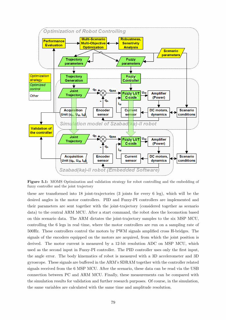
Figure 5.1: MOMS Optimization and validation strategy for robot controlling and the embedding offuzzy controller and the joint trajectory

these are transformed into 18 joint-trajectories (3 joints for every 6 leg), which will be the

desired angles in the motor controllers. PID and Fuzzy-PI controllers are implemented and

their parameters are sent together with the joint-trajectory (considered together as scenario

data) to the central ARM MCU. After a start command, the robot does the locomotion based

on this scenario data. The ARM dictates the joint-trajectory samples to the six MSP MCU,

controlling the 6 legs in real–time, where the motor controllers are run on a sampling rate of

500Hz. These controllers control the motors by PWM signals amplified cross H-bridges. The

signals of the encoders equipped on the motors are acquired, from which the joint position is

derived. The motor current is measured by a 12-bit resolution ADC on MSP MCU, which

used as the second input in Fuzzy-PI controller. The PID controller uses only the first input,

the angle error. The body kinematics of robot is measured with a 3D accelerometer and 3D

gyroscope. These signals are buffered in the ARM’s SDRAM together with the controller related

signals received from the 6 MSP MCU. After the scenario, these data can be read via the USB

connection between PC and ARM MCU. Finally, these measurements can be compared with

the simulation results for validation and further research purposes. Of course, in the simulation,

the same variables are calculated with the same time and amplitude resolution.

79

This system is tested (see Section 5.4), and it fulfills the original mission: enable the vali-

dation of the optimized fuzzy driving.

Figure 5.2: Block diagram of the embedded controllers of Szabad(ka)-II (right side) and the scenariomanagement in Matlab environment (left side)

5.3 Fuzzy-PI Motor Controller Implementation

5.3.1 Calculation and Memory Resource

Not only in the case of fuzzy systems, but generally in all programs, there is some freedom

of implementation between more calculation less memory usage and less calculation with more

memory usage strategies. In the fuzzy controller systems there is three possible ways:

1. Complete calculation from the beginning till the end with least amount of memory. Cal-

culation is used in all three parts: fuzzification, rule-base inference system, defuzzification.

2. Calculation with pre-computed membership functions, which also can be considered as a

lookup table. This kind of realization makes sense, when the membership functions are

fairly complicated and it is worth to pre-calculate them and store them in the memory.

3. Without calculations, with the highest amount of memory usage, where for every output

belongs one lookup table, which is actually the fuzzy surface. This approach can be

applied when there is enough computation memory and the fast calculation is the main

priority, which can be performed in a few steps.

Hereupon, this paper will only deal with the solution under the point 3). The memory size

required for the lookup table MLUT calculated based on the equation 5.1,

MLUT [byte] = NO ·RO/8 · (2RI )NI (5.1)

which depends on the following properties of the fuzzy controller:

• NI Number of inputs, the dimensionality of the lookup table is the same as the number

of inputs (mostly one, two or three)

80

• RI [bit] The resolution of the inputs. In embedded systems the variable and calculations

are usually integer based, especially in case of low-power processors. Accordingly, the

resolution can be 8, 10, 12, or 16-bit.

• RO [bit] The resolution of the output variables, similarly as the inputs

• NO Number of outputs, usually one or a few.

The most critical part is the parameters with exponent, i.e. the number of inputs and bit

resolution. For example a 16 bit resolution can cause implementation problems: the memory

needed for a fuzzy system’s lookup table with one input and two outputs with 16bit resolution

is MLUT = 1 · 16/8 · (216)2 = 8[Gbyte]. Ir can be seen that, neither the lookup table solution is

not that simple, since it’s not easy to calculate, store and search 8Gbyte of data, especially in a

small embedded system. Of course compromises can be drown, using lesser memory, but it will

result in more calculation like followings:

• The lookup table can be compressed either with or without data loss

• Leaving out the unused portions of the table (example if the input is 16bit, but the real

domain is smaller)

• Usage of not linear resolution, which in the insensitive parts of the fuzzy stores samples

in larger increments

• Storing the values in smaller resolution than the inputs, using interpolation

5.3.2 Limitations and Embedding of Fuzzy LUT Controller

The resource limitations of the fuzzy motor controller have been defined based on the general

properties of the MSP micro-controller Texas-Instruments (2012): MSP430F2618, 16MHz, 16-

Bit Ultra-Low-Power MCU, 116kB Flash, 8KB RAM, 12-Bit ADC. The maximum of sampling

and control frequencies is 500Hz. The sufficiency of these frequencies has been proven earlier.

Therefore, n=16MHz/500Hz=32000 cycles are available for one sample, which shall be enough

for the three fuzzy controller cycles attached to the three joints. For one control cycle the

following operations shall be executed:

• Control inputs (for three joints)

– Reading the desired angle from the pre-defined joint-trajectory.

– Reading the actual angle by processing the encoder signals

– Reading the actual motor currents from the ADC

• Running the controller (for three joints)

– Calculation of the angle error, and quantization

– Quantization of the current values

– Determination of the index values of the fuzzy LUT

– Reading the output value from the fuzzy LUT that is stored in the flash memory

81

– (Do integration, if PI type controller is applied)

– Quantization for the PWM output

• Control output (for three joints)

– Setting the new PWM value

• Data acquisition and sending

– Buffering and sending the actual values (measured angle, motor current, PWM duty

cycle)

The micro-controller is equipped with a 12-bit ADC, therefore 12 bits is the theoretical

maximum resolution for the inputs. However, only RI = 8 bit length input is the appropriate

choice, since the 116 Kb flash memory can contain a 64 Kb Fuzzy-LUT beside the program.

This is enough for a NI = 2 input, RO = 8 bit output resolution (NO = 1 output) fuzzy search

table: MLUT = 188(28)2 = 64Kb. It is possible to share the resolution between the two inputs

in an asynchronous manner, for example: the angle error, which is more sensitive, could have

RI1 = 10 bit length, therefore for the resolution of the current RI2 = 6 bit will remain, but the

size of the search table will not change: MLUT = NORO8 (2RI12RI2) = 18

8(21026) = 64Kb.

The fuzzy surface is depicted in Fig. 5.3 (top graph), where the resolution is 10 × 6 × 8bit

after the quantization. The middle and bottom panels of Fig. 5.3 show the projection of

the middle critical part (input 1) of the angle error. The discrete pattern of the values can

be observed compared to the continuous case. Similarly, the 10 and 8bit resolutions can be

compared. However, the simulation results did not show significant differences between the two

solutions.

The LUT based fuzzy controller has also been implemented in the simulation environment,

and a switch is used to select between the original fuzzy controller (using Fuzzy Inference

Systems in Simulink with 64-bit resolution) and the LUT version of the controller. Therefore,

I could analyze the effect of the selected controller over the multi-objective quality of the robot

walking. In the case of the LUT-based control, 1-3% difference was observed compared to the

original 64-bit resolution controller. This result was expected, and I accepted it. For comparison

purpose, the error of a 6-bit resolution fuzzy LUT compared to the original 64-bit resolution is

2-5% Kecskes et al. (2015a).

5.4 Comparison Results of Original and Optimized Driving

The old driving systems with the non-optimized P controller have been compared with the

optimized Fuzzy-PI control solution, which was optimized with the simulation model validated

by the old version (described in Chapter 2). In both experiments, the same straight-forward

walking was performed on Szabad(ka)-II robot using the same length walk cycle.

One of the substantial problems of the old driving was the different time resolution of

trajectory curve (approximately 20Hz) and the controlling frequency (500Hz). Therefore the

used P controller followed rectangular-shaped desired signals, which lead to a jerky oscillating

dynamics. This can be observed in the shape of motor current and control voltage in the left

graphs of Fig. 5.4.

82

Figure 5.3: Fuzzy LUT designed for the motor controller (top graph), 10 bit resolution for angle error(left graph), and 8 bit resolution for angle error (right graph).

The quality of a trajectory curve is generally associated with the energy-efficiency, like in

Deb and Miettinen (2008). For the benefit of this research, I performed a simple comparison:

the average walking speed and the electric power consumption could be calculated, and the ra-

tio of these values gives a quantitative representation of the driving efficiency. Table 5.1 shows

the results: the optimized driving (”2016”) produces 27% faster movement with, 10% smaller

energy consumption, and thus 39% greater efficiency.

Table 5.1: Quality Comparison of two driving solution

Quality Property ”2011” driving ”2016” driving benefit

Average walking velocity (v) 6.21cm/s 7.87cm/s +27%Average Electric Power Consumption (p) 27.1W 24.4W −10%Effectivity (v/p) 0.23cm/J 0.32cm/J +39%

83

Figure 5.4: Comparing hexapod walking by the old ”2011” in left side and new (optimized) ”2016”driving mechanism in right side; the number in parentheses after symbols means (leg number, jointnumber)

5.5 Discussion and Conclusion

Since the simulation model of the robot has been validated, the optimization of the driving al-

gorithm could be elaborated which resulted in improved leg-trajectories and motor controllers.

The research has not been finished, however it could be seen that even these results show the

effect of the quality control (Table 5.1). Based on the simulation and experimental results, I

84

concluded, that it is not worth to develop a robot driving system without performing the nec-

essary calculations and simulations related to the control requirements and resources, sampling

requirement and leg-trajectory properties and parameters first.

To avoid systematic errors in modeling of embedded software of a mobile robot, the following

conditions must be met (In the simulation model of Szabad(ka)-II robot these conditions have

been met.):

• Exactly the same control algorithm or program must run in both places. The Szabad(ka)-

II robot has a LUT based fuzzy implementation because of the limited micro-controller’s

resource. Its mathematical effect, as well as the effect of calculations in the microprocessor

(usually on the basis of integers) should also be part of the model.

• It must be ensured that both the real-time embedded systems and its simulations have

the same sampling frequencies. It is worth checking the accuracy of the internal clocks of

embedded systems because they may deviate from the nominal value.

• In the modeling of controller the resolution and noise level of used sensors (e.g. 16-bit

accelerometer) and resolution of actuator signals (e.g. 8-bit PWM amplifier module)

should be take into account.

The controller in the simulation model of (Kim et al., 2011) is also incorporated in the

form of a LUT. In their robot, the fuzzy LUT controller can significantly reduce the required

calculation time (to 20%).

5.6 Theses Summary

5.6.1 Thesis 5

By measuring the quality of the drive control, it is possible to check whether the

elaborated fuzzy-based control is of better quality than other controllers (such as

classic PID controller). The comparison tests should be performed on the reference

controllers with their best possible settings.2

The feedback of the motor current to the fuzzy controller enables the option of

providing a softer (nonlinear) or even inverse drive. The following supplementary

rules can be set: if the motor current is greater than the nominal or any normal

value the actuator voltage can be driven strongly towards the direction that drives

the motor in the same direction as the load torque does to reduce the electric motor

torque thus reducing the motor current. This is a reverse voltage direction from

the general follow-up control direction. The fuzzy surface shown in the figure 4.5

demonstrates such a controlling rule where the first input is the angle error, the

second input is the motor current, and the output is the actuator voltage.

In the case of Szabad(ka)-II walker robot the optimized Fuzzy-PI controller reached an

average of 20% better global fitness than the optimized PID controller.

For the Szabad(ka)-II robot, the complete optimized system achieved 27% faster locomotion

and 10% less power consumption compared to an earlier, non-optimized program.

2To find the best possible parameters, the same optimization method is recommended for a fair comparison.

85

Comparison to other research results

(Santos et al., 1996) also compared Fuzzy-PID controllers to the traditional PID controller.

Although the parameters of PID controller were determined by a classical tuning method

(Ziegler-Nichols method) and not by a search algorithm. Most researchers do not compare

their fuzzy-based controller performance to a simple PID or PI, for example (Mazhari et al.,

2008) therefore, the advantage of fuzzy logic is not fully elaborated.

Similarly, in study of (Wang et al., 2009) the motor current was returned to the fuzzy controller

but the authors did not explicated in detail the role of the motor current in the controlling.

86

6 Conclusion

This research presents the control development of a walker robot, testing on the Szabad(ka)-II

hexapod robot. The developed simulation model becomes useful for robot driving improvement

because the drive-control became faster and cheaper explored with the model than with the

real robot.

The validated model reached the predefined requirements with the reservation for the dis-

closed imperfections: some structure imperfections of the robot can be identified on the basis of

the validation process and the simulation results. The gear-lash is the most critical mechanical

imperfection of the Szabad(ka)-II robot, which deteriorates the quality of the robot motion.

The presented validation procedure in chapter 2 revealed that Szabad(ka)-II robot with some

structural improvements could be a more applicable device having higher motion quality and

smaller energy consumption.

The design variables of the robot walking problem can include both parameters of the leg

trajectory and the controller simultaneously (in this dissertation a PID and Fuzzy-PI controller).

In case of Szabad(ka)-II robot altogether it creates 17 design variables. Generally it is a multi-

variable, single-objective, non-differentiable, non-linear, non-continuous optimization problem.

Single-objective, if the multi-objective dimension is aggregated as it proposed in this disserta-

tion, otherwise multi-objective. A method introduced in Chapter 3 was developed for selecting

the best potential evolutionary optimization method used for a given problem. The artificial

test functions for a benchmark were created including the mathematical characteristics that

are interesting or typically describe the examined robot optimization problem. The PSO and

PSO-PS hybrid methods were selected as best for the function having similar characteristics as

the robot problem. The PSO-PS proves to be effective compared with the earlier optimization

attempts using GA, giving significantly better results, for both PID and fuzzy type controllers.

A simple Fuzzy-PI controller was developed in Chapter 3, which reached better walking

quality than the traditional PID controller after the optimization procedures under similar

conditions. This controller use the motor current as the second input and realize a softer

control behavior against high torque values.

The quality definition related to hexapod walking as a multi-objective approach was de-

scribed in Chapter 4. It presents how to aggregate the multi-objectives into a scalar value using

preference weights and integrating the multi-scenario type simulation. For simulation models

in which the equipment is intended to perform many or an infinite number of missions, a set of

typical scenarios for the intended use can represent the entire set of scenarios. The preferences

are implemented in a utility function with a bias and exponent pair weights for each objective,

while the scenarios are aggregated with geometrical mean. Finally, a bias-weighted product type

utility function is proposed (BWP). The optimization results show a high divergence between

the optimums for different preferences between the objectives. This raises another optimization

issue, which I believe is an important part of the entire system. The sensitivity or robustness

analysis can be used as an external quality aspect to select the appropriate preferences.

Chapter 5 described the essential aspects that were taken into account during the real-

87

ization procedure of the new driving algorithm of the Szabad(ka)-II hexapod robot. The old

non-optimized walking system was an initial solution created to able to run the robot and take

measurements for the model validation, using a P controller. This old version of driving was

improved by the development and optimization of leg–trajectory and the Fuzzy-PI motor con-

troller. The fuzzy inference system was implemented as a lookup table in the low performance

microcontrollers. Its properties and mathematical effect were addressed in the level of simula-

tion model. Walking efficiency was increased by these efforts, the new driving produces faster

movement with reduced energy consumption under the same environmental conditions.

The quality definition and measurement, optimization, implementation and validation meth-

ods presented in the dissertation are generally applicable in the field of robotics, not just for

six-legged walker robots. Five thesis has been highlighted from many conclusions and results

discussed in this dissertation. The message of these theses can be summarized as follows:

The drive quality of a walker robot can be significantly improved with a good design and quality

optimization performed on a simulation model. For this purpose, the following essential aspects

must be studied:

• The objective functions of the walking quality should be determined so that these can be

measured on the real device.

• The type and structure of controller, the sampling rates, control, and variables to be

measured should be designed taking into account feasible performance and speeds in the

robot’s digital control unit.

• Optimization of the drive control should be performed on a validated model. In the

case of Szabad(ka)-II robot the fuzzy-PI motor control and the static leg trajectory were

optimized.

• The optimum should be calculated simultaneously for multiple scenarios which describe

the typical movements-series of the robot.

88

Bibliography

Abramson, M. A. (2002). Pattern search algorithms for mixed variable general constrainedoptimization problems. Technical report, AIR FORCE INST OF TECH WRIGHT-PATTERSONAFB OH.

Allen, T. J., Quinn, R. D., Bachmann, R. J., and Ritzmann, R. E. (2003). Abstracted biologi-cal principles applied with reduced actuation improve mobility of legged vehicles. IntelligentRobots and Systems, 2003.(IROS 2003). Proceedings. 2003 IEEE/RSJ International Confer-ence on, 2, 1370–1375.

Appl-DSP.com (2011). Szabad(ka) robots. www.szabadka-robot.com.

Arena, P., Fortuna, L., Frasca, M., Patane, L., and Pavone, M. (2006). Implementation and ex-perimental validation of an autonomous hexapod robot. In Proceedings of IEEE InternationalSymposium on Circuits and Systems, pages 401–406.

Augusto, O. B., Bennis, F., and Caro, S. (2012). Multiobjective engineering design optimizationproblems: a sensitivity analysis approach. Pesquisa Operacional , 32(3), 575–596.

Bai, Y., Zhuang, H., and Wang, D. (2007). Advanced fuzzy logic technologies in industrialapplications. Springer Science & Business Media.

Bai, Y., Sun, Z., Quan, L., and Yu, S. (2010). A linear interpolation fuzzy controller withnn compensator for an electro-hydraulic servo system. In Computational Aspects of SocialNetworks (CASoN), 2010 International Conference on, pages 565–568. IEEE.

Bai, Y., Guo, N., and Agbegha, G. (2012). Fuzzy interpolation and other interpolation methodsused in robot calibrations. Journal of Robotics, 2012.

Bailey, S. (2004). Biomimetic Control with a Feedback coupled Nonlinear Oscillator: InsectExperiments, Design Tools, and Hexapedal Robot Adaptation Results. Ph.D. thesis, StanfordUniversity.

Bartsch, S., Birnschein, T., Rommermann, M., Hilljegerdes, J., Kuhn, D., and Kirchner, F.(2012). Development of the six-legged walking and climbing robot spaceclimber. Journal ofField Robotics, 29(3), 506–532.

Braunl, T. (1998). Embedded robotics. Springer .

Burkus, E. and Odry, P. (2007). Autonomous hexapod walker robot ”szabad(ka)”. In IntelligentSystems and Informatics (SISY), IEEE 5th International Symposium on, pages 103–106.

Burkus, E. and Odry, P. (2008). Autonomous hexapod walker robot ”szabad(ka)”. Acta Poly-technica Hungarica, 5(1), 69–85.

Burkus, E., Radosav, D., and Odry, P. (2011). Autonomous hexapod walker robot ”szabad(ka)ii” - software modeling and tools. ITRO 2011, Zrenjanin, Serbia.

Burkus, E., Fodor, J. C., and Odry, P. (2013). Structural and gait optimization of a hexapodrobot with particle swarm optimization. In Intelligent Systems and Informatics (SISY), IEEE11th International Symposium on, pages 147–152.

Carbone, G. (2011). Stiffness analysis and experimental validation of robotic systems. Frontiersof Mechanical Engineering , 6(2), 182–196.

89

Carbone, G. and Ceccarelli, M. (2008a). A low-cost easy-operation hexapod walking machine.International Journal of Advanced Robotic Systems, 5(2), 21.

Carbone, G. and Ceccarelli, M. (2008b). A low-cost easy-operation hexapod walking machine.International Journal of Advanced Robotic Systems, 5(2), 161–166.

Celaya, E. and Albarral, J. L. (2003). Implementation of a hierarchical walk controller forthe lauron iii hexapod robot. In International Conference on Climbing and Walking robots(Clawar 2003), pages 409–416.

Center, W. R. U. (2008). Biologically inspired robotics, case western reserve university. Website.

CMU (2008). Artificial intelligence and applied problem solving from cmu, a world leader inmobile robotics, chiara- the next generation of research robots. http://chiara-robot.org/chiara-brochure-july-2008.pdf.

Collins, J. J. and Stewart, I. N. (1993). Coupled nonlinear oscillators and the symmetries ofanimal gaits. Journal of Nonlinear Science, 3(1), 349–392.

Corke, I. (2001). Robotics toolbox for matlab (release 6). Manufacturing Science and TechnologyPinjarra Hills, Australia.

Csendes, T. (2004). Clustering global optimization program - global. https://www.inf.

u-szeged.hu/~csendes/.

Csendes, T., Pal, L., Sendın, J. O. H., and Banga, J. R. (2008). The global optimization methodrevisited. Optimization Letters, 2(4), 445–454.

Currie, J., Beckerleg, M., and Collins, J. (2010). Software evolution of a hexapod robot walkinggait. International journal of intelligent systems technologies and applications, 8(1), 382–394.

de Melo, L. F., Junior, J. F., and Florino, J. A. C. (2011). Rapid prototyping for mobile robotsembedded control systems. In Advanced Applications of Rapid Prototyping Technology inModern Engineering . InTech.

De Santos, P. G., Garcia, E., and Estremera, J. (2007). Improving walking-robot performancesby optimizing leg distribution. Autonomous Robots, 23(4), 247–258.

de Santos, P. G., Garcia, E., Ponticelli, R., and Armada, M. (2009). Minimizing energy con-sumption in hexapod robots. Advanced Robotics, 23(6), 681–704.

Deb, K. and Miettinen, K. (2008). Multiobjective optimization: Interactive and evolutionaryapproaches, volume 5252. Springer Science & Business Media.

Delcomyn, F. and Nelson, M. E. (2000). Architectures for a biomimetic hexapod robot. Roboticsand Autonomous Systems, 30(1), 5–15.

Ding, X., Wang, Z., Rovetta, A., and Zhu, J. (2010). Locomotion analysis of hexapod robot.Climbing and Walking Robots, pages 291–310.

Duindam, V. (2006). Port-based modeling and control for efficient bipedal walking robots. Ph.D.thesis, University of Twente.

Erden, M. S. (2011). Optimal protraction of a biologically inspired robot leg. Journal ofIntelligent & Robotic Systems, 64(3), 301–322.

Erdogmus, P. and Toz, M. (2012). Serial and Parallel Robot Manipulators - Kinematics, Dy-namics, Control and Optimization. under CC BY 3.0 license.

90

Fadel, G., Haque, I., Blouin, V., and Wiecek, M. (2005). Multi-criteria multi-scenario ap-proaches in the design of vehicles. In 6th World Congresses of Structural and MultidisciplinaryOptimization.

Faulhaber, F. (2005). Precise gearheads efficiency measurement. www.faulhaber.com.

Faulhaber.com (2014). Faulhaber gmbh. www.faulhaber.com.

Fielding, M. R., Dunlop, R., and Damaren, C. (2001). Hamlet: force/position controlled hexa-pod walker-design and systems. In Control Applications, 2001.(CCA’01). Proceedings of the2001 IEEE International Conference on, pages 984–989. IEEE.

Georgiades, C. (2005). Simulation and Control of an Underwater Hexapod Robot . Ph.D. thesis,Department of Mechanical Engineering McGill University, Montreal.

Goldberg, D. E. and Holland, J. H. (1988). Genetic algorithms and machine learning. Machinelearning , 3(2), 95–99.

Gonzalez de Santos, P., Cobano, J. A., Garcia, E., Estremera, J., and Armada, M. (2007).A six-legged robot-based system for humanitarian demining missions. Mechatronics, 17(8),417–430.

GoogleCode (2014). Particle swarm toolbox for matlab. code.google.com/p/psomatlab/.

Grizzle, J., Chevallereau, C., Ames, D., and Sinnet, W. (2010). 3d bipedal robotic walking:Models, feedback control, and open problems. IFAC Proceedings, 43(14), 505–532.

Grzelczyk, D., Stanczyk, B., and Awrejcewicz, J. (2017). Kinematics, dynamics and powerconsumption analysis of the hexapod robot during walking with tripod gait. InternationalJournal of Structural Stability and Dynamics, 17(05), 1740010.

Haavisto, O. and Hyotyniemi, H. (2004). Simulation tool of a biped walking robot model. Espoo,March 2004, Report 138, Helsinki University of Technology .

Hauser, K., Bretl, T., Latombe, J., and Wilcox, B. (2006). Motion planning for a six-legged lunarrobot. The Seventh International Workshop on the Algorithmic Foundations of Robotics, 7,16–18.

Hedar, A.-R. and Fukushima, M. (2006). Tabu search directed by direct search methods fornonlinear global optimization. European Journal of Operational Research, 170(2), 329–349.

Hutter, M. and Naf, D. (2011). Quadruped walking/running simulation. Spring Term. Semester-Thesis in ETH Zurich.

Iagnemma, K. and Dubowsky, S. (2004). Traction control of wheeled robotic vehicles in roughterrain with application to planetary rovers. The international Journal of robotics research,23(10-11), 1029–1040.

Jaen-Cuellar, A. Y., de J. Romero-Troncoso, R., Morales-Velazquez, L., and Osornio-Rios,R. A. (2013). Pid-controller tuning optimization with genetic algorithms in servo systems.International Journal of Advanced Robotic Systems, 10(9), 324.

Jahandideh, H. and Namvar, M. (2012). Use of pso in parameter estimation of robot dynamics;part two: Robustness. In System Theory, Control and Computing (ICSTCC), 2012 16thInternational Conference on, pages 1–6. IEEE.

91

Jakimovski, B., Meyer, B., and Maehle, E. (2009). Self-reconfiguring hexapod robot oscarusing organically inspired approaches and innovative robot leg amputation mechanism. In-ternational Conference on Automation, Robotics and Control Systems, ARCS 2009, Orlando,USA.

Janrathitikarn, O. and Long, L. N. (2008). Gait control of a six-legged robot on unlevel terrainusing a cognitive architecture. Aerospace Conference, 2008 IEEE , pages 1–9.

Jovanovic, D., Hilderink, G. H., and Broenink, J. F. (2002). A case study for tooling the designtrajectory of embedded control systems. In 3rd PROGRESS Workshop on Embedded Systems2002 - Utrecht, Netherlands. STW Technology Foundation.

Kar, D. C. (2003). Design of statically stable walking robot: a review. Journal of RoboticSystems, 20(11), 671–686.

Kecskes, I. (2017). Matlab source code of robust optimization of multi-scenario multi-objective function. http://appl-dsp.com/wp-content/uploads/2014/03/mlib_MSMO_

optimization.zip.

Kecskes, I. and Odry, P. (2009a). Full kinematic and dynamic modeling of ”Szabad(ka)-Duna”hexapod. In Intelligent Systems and Informatics (SISY), IEEE 7th International Symposiumon, pages 215–219.

Kecskes, I. and Odry, P. (2009b). Fuzzy controlling of hexapod robot arm with coreless dcmicromotor. In XXIII. MicroCAD, Miskolc, 2009 March, pages 19–20.

Kecskes, I. and Odry, P. (2009c). Walk optimization for hexapod walking robot. In Proceedingsof 10th International Symposium of Hungarian Researchers on Computational Intelligenceand Informatics (CINTI), Budapest, Hungary, November , pages 12–14.

Kecskes, I. and Odry, P. (2010). Protective fuzzy control of hexapod walking robot driver incase of walking and dropping. In Computational Intelligence in Engineering , pages 205–217.Springer.

Kecskes, I. and Odry, P. (2012). Fuzzy route control of dynamic model of four-wheeled mobilerobot. In Logistics and Industrial Informatics (LINDI), 4th IEEE International Symposiumon, pages 215–220.

Kecskes, I. and Odry, P. (2013). Simple definition of adequate fixed time-step size of Szabad(ka)-II robot model. In Computational Cybernetics (ICCC), IEEE 9th International Conferenceon, pages 315–320.

Kecskes, I. and Odry, P. (2014). Optimization of PI and fuzzy-PI controllers on simulationmodel of Szabad(ka)-II walking robot. Int. J. Adv. Robot. Syst., 11, 186.

Kecskes, I., Szekacs, L., Fodor, J. C., and Odry, P. (2013). PSO and GA optimization methodscomparison on simulation model of a real hexapod robot. In Computational Cybernetics(ICCC), IEEE 9th International Conference on, pages 125–130.

Kecskes, I., Burkus, E., and Odry, P. (2014). Swarm-based optimizations in hexapod robot walk-ing. In Applied Computational Intelligence and Informatics (SACI), IEEE 9th InternationalSymposium on, pages 123–127.

Kecskes, I., Szekacs, L., and Odry, P. (2015a). Lookup table based fuzzy controller implemen-tation in low-power microcontrollers of hexapod robot szabad (ka)-ii. In 3rd InternationalConference & Workshop Mechatronics in Practice and Education–MECHEDU , pages 76–81.

92

Kecskes, I., Burkus, E., Bazso, F., and Odry, P. (2015b). Model validation of a hexapod walkerrobot. Robotica, 35(2), 419–462.

Kecskes, I., Odry, A., Burkus, E., and Odry, P. (2016). Embedding optimized trajectory andmotor controller into the Szabad(ka)-II hexapod robot. In Systems, Man, and Cybernetics(SMC), 2016 IEEE International Conference on, pages 001417–001422.

Kecskes, I., Burkus, E., Kiraly, Z., Odry, A., and Odry, P. (2017a). Competition of motorcontrollers using a simplified robot leg: Pid vs fuzzy logic. In Mathematics and Computersin Sciences and in Industry (MCSI), 2017 Fourth International Conference on, pages 37–43.IEEE.

Kecskes, I., Burkus, E., Kiraly, Z., Odry, A., and Odry, P. (2017b). Competition of motorcontrollers using a simplified robot leg pid vs fuzzy logic. In 4th International Conference onMathematics and Computers in Sciences and Industry (MCSI).

Kennedy, B., Aghazarian, H., Cheng, Y., Garrett, M., Hutsberger, T., Magnone, L., Okon, A.,and Robinson, M. (2002). Limbed excursion mechanical utility rover: LEMUR II. In 53rdInternational Astronautical Congress.

Kikuuwe, R., Takesue, N., Sano, A., Mochiyama, H., and Fujimoto, H. (2005). Fixed-stepfriction simulation: from classical coulomb model to modern continuous models. In IntelligentRobots and Systems, 2005.(IROS 2005). 2005 IEEE/RSJ International Conference on, pages1009–1016. IEEE.

Kim, J., Kim, Y.-G., and An, J. (2011). A fuzzy obstacle avoidance controller using a lookup-table sharing method and its applications for mobile robots. International Journal of Ad-vanced Robotic Systems, 8(5), 39–48.

Kirkpatrick, S., Gelatt, C. D., and Vecchi, M. P. (1983). Optimization by simulated annealing.science, 220(4598), 671–680.

Konyev, M., Palis, F., Zavgorodniy, Y., Melnikov, A., Rudskiy, A., Telesh, A., SCHMUCKER,U., and Rusin, V. (2008). Walking robot ANTON: Design, simulation, experiments. In Proc.of 11th Int. Conf. on Climbing and Walking Robots (CLAWAR), pages 922–929.

Krishnan, R. (2001). Electric Motor Drives Modeling, Analysis and Control . Prentice Hall.

Kubelka, V., Oswald, L., Pomerleau, F., Colas, F., Svoboda, T., and Reinstein, M. (2014).Robust data fusion of multimodal sensory information for mobile robots. Journal of FieldRobotics, (Early View).

Kubler, L., Henninger, C., and Eberhard, P. (2005). Multi-criteria optimization of a hexapodmachine. In Advances in Computational Multibody Systems, pages 319–343. Springer.

Lewinger, W. A., Branicky, M. S., and Quinn, R. D. (2005). Insect-inspired, actively compli-ant hexapod capable of object manipulation. Proceedings CLAWAR 2005, 8th InternationalConference on Climbing and Walking Robots, 8, 65–72.

Lin, B. S. and Song, S.-M. (2001). Dynamic modeling, stability, and energy efficiency of aquadrupedal walking machine. Journal of Field Robotics, 18(11), 657–670.

Lin, P.-C., Komsuoglu, H., and Koditschek, D. E. (2005). A leg configuration measurementsystem for full-body pose estimates in a hexapod robot. Robotics, IEEE Transactions on,21(3), 411–422.

93

Ma, O., Wang, J., Misra, S., and Liu, M. (2004). On the validation of spdm task verificationfacility. Journal of Field Robotics, 21(5), 219–235.

Majhi, B. and Panda, G. (2011). Robust identification of nonlinear complex systems using lowcomplexity ann and particle swarm optimization technique. Expert Systems with Applications,38(1), 321–333.

Marijt, R. (2009). Multi-objective Robust Optimization Algorithms for Improving Energy Con-sumption and Thermal Comfort of Buildings. Master’s thesis, Leiden Institute for AdvancedComputer Science, Leiden University.

Mastacan, L. and Dosoftei, C.-C. (2013). Level fuzzy control of three-tank system. In ControlSystems and Computer Science (CSCS), 2013 19th International Conference on, pages 30–35.IEEE.

MathWorks (2014a). Find minimum of function using pattern search. www.mathworks.com/

help/gads/patternsearch.html.

MathWorks (2014b). Genetic algorithm. www.mathworks.com/discovery/

genetic-algorithm.html.

MathWorks (2014c). Simulated annealing. www.mathworks.com/discovery/

simulated-annealing.html.

Mazhari, S. A., Kumar, S., and Ieee, M. (2008). Heuristic search algorithms for tuning puma560 fuzzy pid controller. International Journal of Electrical and Information Engineering ,2(9), 2024–2033.

Melendez, A. and Castillo, O. (2013). Evolutionary optimization of the fuzzy integrator in anavigation system for a mobile robot. Recent Advances on Hybrid Intelligent Systems, pages21–31.

Melluso, M. (2012). A theoretical and experimental approach of fuzzy adaptive motion controlfor wheeled autonomous nonholonomic vehicles. ISRN Robotics, 2013.

Mirjalili, S. and Lewis, A. (2015). Novel frameworks for creating robust multi-objective bench-mark problems. Information Sciences, 300, 158–192.

Nelson, A. L., Barlow, G. J., and Doitsidis, L. (2009). Fitness functions in evolutionary robotics:A survey and analysis. Robotics and Autonomous Systems, 57(4), 345–370.

Odry, A., Burkus, E., Kecskes, I., Fodor, J., and Odry, P. (2016). Fuzzy control of a two-wheeled mobile pendulum system. In Applied Computational Intelligence and Informatics(SACI), 2016 IEEE 11th International Symposium on, pages 99–104. IEEE.

Odry, A., Fuller, R., Rudas, I. J., and Odry, P. (2018). Kalman filter for mobile-robot atti-tude estimation: Novel optimized and adaptive solutions. Mechanical Systems and SignalProcessing , 110, 569–589.

Odry, P., Burkus, E., and Sram, N. (2006). Hexapod robot as an algorithm developing platform.Available from: http://cneuro.rmki.kfki.hu/events/past/robot#odry.

Ohroku, H. and Nonami, K. (2008). Omni-directional vision and 3d animation based teleop-eration of hydraulically actuated hexapod robot comet-iv. Transactions Of The Japan FluidPower System Society 01/2009 , 40(6).

94

Pap, Z., Kecskes, I., Burkus, E., Bazso, F., and Odry, P. (2010). Optimization of the hexapodrobot walking by genetic algorithm. In Intelligent Systems and Informatics (SISY), IEEE8th International Symposium on, pages 121–126.

Pedersen, M. E. H. (2010). Good parameters for particle swarm optimization. Hvass Lab.,Copenhagen, Denmark, Tech. Rep. HL1001 .

Porta, J. M. and Celaya, E. (2004). Reactive free-gait generation to follow arbitrary trajectorieswith a hexapod robot. Robotics and Autonomous Systems, 47(4), 187–201.

Pratihar, D. K., Deb, K., and Ghosh, A. (2000). Optimal turning gait of a six-legged robotusing a ga-fuzzy approach. AI EDAM , 14(3), 207–219.

Pratihar, D. K., Deb, K., and Ghosh, A. (2002). Optimal path and gait generations simulta-neously of a six-legged robot using a ga-fuzzy approach. Robotics and Autonomous Systems,41(1), 1–20.

Precup, R.-E. and Hellendoorn, H. (2011). A survey on industrial applications of fuzzy control.Computers in Industry , 62(3), 213–226.

Precup, R.-E., David, R.-C., Petriu, E. M., Radac, M.-B., Preitl, S., and Fodor, J. (2013). Evolu-tionary optimization-based tuning of low-cost fuzzy controllers for servo systems. Knowledge-Based Systems, 38, 74–84.

Ramanathan, G., Morandi, B., West, S., and Meyer, B. (2010). Scoop for robotics, implement-ing bio-inspired hexapod locomotion, eth zurich. http://se.inf.ethz.ch/old/projects/

ganesh_ramanathan/report.pdf.

Rao, R. V., Savsani, V. J., and Vakharia, D. (2011). Teaching–learning-based optimization:a novel method for constrained mechanical design optimization problems. Computer-AidedDesign, 43(3), 303–315.

Rao, S. S. (2009). Engineering optimization: theory and practice. John Wiley & Sons.

Rashedi, E. (2011). Matlab code for gravitational search algorithm. https://it.mathworks.

com/matlabcentral/fileexchange/27756-gravitational-search-algorithm--gsa-.

Rashedi, E., Nezamabadi-Pour, H., and Saryazdi, S. (2009). Gsa: a gravitational search algo-rithm. Information sciences, 179(13), 2232–2248.

Regenstein, K., Kerscher, T., Birkenhofer, C., Asfour, T., Zllner, J., and Dillmann, R. (2007).A modular approach for controlling mobile robots. In Proc. of CLAWAR 2007, 10th Inter-national Conference on Climbing and Walking Robots.

Renda, F., Giorelli, M., Calisti, M., and Cianchetti, M. (2014). Dynamic model of a multibend-ing soft robot arm driven by cables. IEEE Transactions on Robotics, 30(5), 1109–1122.

Ricardo, D. and Costa, C. (2010). Hexapod Locomotion: a Nonlinear Dynamical Systems Ap-proach. Ph.D. thesis, Universidade do Minho, Escola de Engenharia.

Rios, L. M. and Sahinidis, N. V. (2013). Derivative-free optimization: a review of algorithms andcomparison of software implementations. Journal of Global Optimization, 56(3), 1247–1293.

Rone, W. S. and Ben-Tzvi, P. (2014). Continuum robot dynamics utilizing the principle ofvirtual power. Transactions On Robotics, 30(1), 275–287.

Rudas, J. and Fodor, J. (2008). Intelligent systems. Int. J. of Computers, Communications andControl , 3, 132–138.

95

Sakr, Z. and Petriu, E. M. (2007). Hexapod robot locomotion using a fuzzy controller. InRobotic and Sensors Environments, 2007. ROSE 2007. International Workshop on, pages1–5. IEEE.

Santos, M., Dormido, S., and De La Cruz, J. (1996). Fuzzy-pid controllers vs. fuzzy-pi con-trollers. In Fuzzy Systems, 1996., Proceedings of the Fifth IEEE International Conferenceon, volume 3, pages 1598–1604. IEEE.

Saranli, U., Buehler, M., and Koditschek, D. E. (2001). RHex: A simple and highly mobilehexapod robot. The International Journal of Robotics Research, 20(7), 616–631.

Shoorehdeli, M. A., Teshnehlab, M., and Sedigh, A. K. (2009). Training anfis as an identifierwith intelligent hybrid stable learning algorithm based on particle swarm optimization andextended kalman filter. Fuzzy Sets and Systems, 160(7), 922–948.

Silva, M. F. and Machado, J. T. (2007). A historical perspective of legged robots. Journal ofVibration and Control , 13(9-10), 1447–1486.

Silva, M. F. and Machado, J. T. (2012). A literature review on the optimization of leggedrobots. Journal of Vibration and Control , 18(12), 1753–1767.

Sobhan, P., Kumar, G. N., Priya, M. R., and Rao, B. V. (2009). Look up table based fuzzylogic controller for unmanned autonomous underwater vehicle. In Advances in Computing,Control, & Telecommunication Technologies, 2009. ACT’09. International Conference on,pages 497–501. IEEE.

Tanaka, K., Ikeda, T., and Wang, H. O. (1996). Robust stabilization of a class of uncertainnonlinear systems via fuzzy control: quadratic stabilizability, hinf control theory, and linearmatrix inequalities. IEEE Transactions on Fuzzy systems, 4(1), 1–13.

Tedeschi, F. and Carbone, G. (2014). Design issues for hexapod walking robots. Robotics, 3(2),181–206.

Texas-Instruments (2012). Msp430f261x. http://www.ti.com/lit/ds/symlink/

msp430f2618.pdf.

Trochim, W. M. (2006). Types of reliability in the research methods knowledge base, 2ndedition. http://www.socialresearchmethods.net/kb/reltypes.php.

Ullah, I., Ullah, F., Ullah, Q., and Shin, S. (2013). Integrated tracking and accident avoidancesystem for mobile robots. International Journal of Control, Automation and Systems, 11(6),1253–1265.

Veres, J. (2013). Bio-Inspired Low-Cost Robotic Joint With Reduced Level Of Backlash AndA Novel Approach - The Emulated Elastic Actuator . Ph.D. thesis, Faculty of InformationTechnology, Pazmany Peter Catholic University.

Von Twickel, A., Hild, M., Siedel, T., Patel, V., and Pasemann, F. (2012). Neural control of amodular multi-legged walking machine: Simulation and hardware. Robotics and AutonomousSystems, 60(2), 227–241.

Wai, R.-J. (2003). Robust fuzzy neural network control for nonlinear motor-toggle servomech-anism. Fuzzy sets and systems, 139(1), 185–208.

Wang, M.-S., Kung, Y.-S., and Tu, Y.-M. (2009). Fuzzy logic control design for a stair-climbingrobot. International Journal of Fuzzy Systems, 11(3), 174–182.

96

Woering, R. (2011). Simulating the ”first steps” of a walking hexapod robot . Ph.D. thesis,Master’s thesis, Technische Universiteit Eindhoven, Eindhoven, CST 2010.

Wong, C.-C., Wang, H.-Y., Li, S.-A., and Cheng, C.-T. (2007). Fuzzy controller designed by gafor two-wheeled mobile robots. International Journal of Fuzzy Systems, 9(1), 22–30.

Wong, C.-C., Wang, H.-Y., and Li, S.-A. (2008). Pso-based motion fuzzy controller design formobile robots. International Journal of Fuzzy Systems, 10(1), 284–292.

Yanhong, B., Zhijuan, Z., Zhiyi, S., and Long, Q. (2013). A linear interpolation fuzzy controllerfor a boiler pressure control system. IFAC Proceedings Volumes, 46(5), 650–654.

Yarpiz (2015a). Matlab implementation of tlbo for global opti-mization. https://it.mathworks.com/matlabcentral/fileexchange/

52863-teaching-learning-based-optimization--tlbo-.

Yarpiz (2015b). Tabu search (ts) in matlab. http://yarpiz.com/243/ypea116-tabu-search.

Zheng, T., Godage, I. S., Branson, D. T., Kang, R., Guglielmino, E., Medrano-Cerda, G. A., andCaldwell, D. G. (2013). Octopus inspired walking robot: Design, control and experimentalvalidation. In Robotics and Automation (ICRA), 2013 IEEE International Conference on,pages 816–821. IEEE.

Zhu, L., Deb, K., and Kulkarni, S. (2014). Optimization of multi-scenario problems using multi-criterion methods: A case study on byzantine agreement problem. COIN Report Number2014002 .

Zielinska, T. and Heng, J. (2002). Development of a walking machine: mechanical design andcontrol problems. Mechatronics, 12(5), 737–754.

97

.1 Appendix: Comparison of Szabad(ka)-II with similar robots

From the hexapod robots listed in Table 1.2 we selected those which were close to the predefinedrequirements, and expectations, we highlighted characteristics relevant for our study. Selectionwas based on the structure and purpose of the robot. From Table 1.2, the following robots wereselected for further discussion: Hamlet, LAVA, SILO 6, LEMUR II, Anton and SpaceClimber.

.1.1 Hamlet

Mechanically sophisticated six-legged robot Hamlet Fielding et al. (2001) driven by servo motorswas developed to test the effectiveness of combined force and position control to achieve robust,adaptable walking over rough and unknown environments. The robot weighs 13 kg. The distancebetween the front and rear legs, measured at their axis in the body is 400mm. The robot hasa carbon-fiber-coated cardboard body. Six identical legs are made of aluminum and the jointsare driven with identical 10W DC motors mounted to reductors with a ratio of 1:246. Flexiblecouplings were used to transfer the power from the reductors to the plastic bevel gears.Hamlet and Szabad(ka)-II are most similar in their construction, but differ in the following mainproperties: Szabad(ka)-II with its full equipment weighs only 6.5 kg. The distance between thefront and rear axes of the legs is 320mm, that is 20 % shorter than in Hamlet. The legs and thebody of Szabad(ka)-II are milled out from aluminum and steel elements, and the electronics arelocated inside the body, while Hamlet’s chassis is a sandwich of carbon fiber over corrugatedcardboard and only the legs are made of aluminum.Our previous results Kecskes and Odry (2010) helped us to select drive elements of Szabad(ka)-II. Based on these simulations appropriate servo motor / gearbox pairs could be determined.This was required to ensure proper torques (Table 1.1). Szabad(ka)-II uses different servomotors, while Hamlet was built with identical servo motor / regulator pairs. Among others,the goals were to reduce the overall costs and simplify the structure. For this reason smallersteel bevel gears were chosen. The bevel gears and the motors were connected without flexiblecouplings.

.1.2 LAVA

In the case of LAVA Zielinska and Heng (2002) the first two joints of the legs (closer to thebody) are driven with an inverse differential gear drive system. Depending on the rates at whichthe two gear driving motors rotate, the legs may be lifted, swung or simultaneously performboth motions. This solution has two advantages. First, the lifting and swinging has a commongeometrical pivot point and owing to this, the kinematic modeling is simpler. Second, during theleg swing and leg lift motions, both motors work simultaneously to achieve the desired motion.Thus, when walking, none of the motors is idle. In case of vertical leg motions, when the largesttorque is applied, both motors lift the robot at the same time. Such a solution results both inweight and power savings.In brief, the inverse differential gear drive system has some advantages in several areas. ForSzabad(ka)-II, the traditional solution was chosen because in this case the location of the motorsmakes the layout of the other elements proportional. While designing Szabad(ka)-II it wasespecially important to place the electronics inside the robot’s body. In addition, an importantrequirement was to keep the drive mechanism as simple as possible, because the more complexa structure is, the more difficult it is to achieve a precise operation.LAVA’s another interesting mechanical solution is that it uses worm gears instead of bevelgears. The advantage of the worm gear over the bevel gear is that the former has self-lockingproperties. This feature is important because when the robot is standing, it can hold theposition of the joints without consuming energy. In case of planetary gearheads the reversetransmission of torque from the joint to the motor can only be achieved with great losses. Onthe other hand, a DC motor can be used as a brake by short-circuiting its inputs. Thus, thecombined effects of the planetary reductor’s efficiency in the case of reverse torques and the

98

shorted motor inputs act as the worm gear’s self-locking effect, so energy can be saved whilestanding without using worm gears. Another reason for not using worm gears was that theapplied planetary gearheads already provided appropriate reduction. There was no need foradditional electronic components to short the windings of the motors because the integratedfull-bridge drive circuit (Texas Instruments DRV8801) used in the robot was suitable for thistask.

.1.3 SILO6

Similarly to LAVA, SILO6 Gonzalez de Santos et al. (2007) also uses an inverse differential geardrive system. However, in SILO6 the gear system drives the two joints located further fromthe body. This solution made it possible to place all three motors closer to the center. It isimportant to protect the motors since the primary use of SILO6 is mine deactivation.In the process of developing SILO6 another goal was to minimize energy consumption whilewalking on uneven terrain. In the case of the computer model it was assumed that the robot’scenter of gravity (COG) moves along a horizontal straight line with a constant speed. In theequations of motion the inertia was also included which arises while the leg is in motion.In the case of Szabad(ka)-II various optimization methods on the dynamic simulation modelwere being used to minimize power consumption. In the first step optimization was applied tothe servo controller and the walking algorithm’s path planner.

.1.4 LEMUR II

This hexapod robot was developed by NASA Kennedy et al. (2002). It was originally developedfor space applications, but is currently being tested in terrestrial environment. The layout ofthe system consists of six 4 degree-of-freedom limbs arranged axisymmetrically around a hexag-onal body platform. Besides the three typical degrees of freedom it also has a fourth DOFwhich enables the legs to serve as arms. These arms are not only used for walking but also formounting. Interchangeable tools can be attached to the end of the arms.LEMUR II has identical MAXON motors with 13mm diameter, planetary reductors and en-coders. It uses an inverse differential gear drive system. For mechanical torque transfer, besidesthe planetary reductor, a harmonic drive was also included. A harmonic drive is capable oftransferring higher torques with less backslash Kennedy et al. (2002).

.1.5 ANTON

Hexapod robot ANTON Konyev et al. (2008) is the successor of SLAIR 2. In case of SLAIR2 differential joints were used but the reduction between the motors and the joints was solvedwith home-made spur gearheads, not with planetary ones. Instead of encoders potentiometerswere implemented mounted on the main shafts of the joints behind the reductors, not on themotors. ANTON 2 uses an upgraded differential joint where the joint centers in the legs areshifted relative to each other. In this case, torque transmission was solved with a wire structure.Besides the 6× 3 DOFs in the legs, the robot’s body received additional 3× 2 DOFs. Becauseof additional degrees of freedom, the body and the head are capable of rotating relative to eachother at 3 points.

.1.6 SpaceClimber

Probably the most advanced robot among the devices in this section is SpaceClimber Bartschet al. (2012). It is a six-legged, bio-inspired, energy-efficient and adaptable free climbing robotintended for mobility on steep gradients. Its final mission is to provide a system for extrater-restrial surface exploration missions, paying special attention to mobility in lunar craters toretrieve or analyze scientific samples from crater-interiors.The robot weighs 23 kg. Its dimensions (in normal posture) are 850×1000×220mm[L×W×H].The length of the leg segments as well as the size of the body and the positions of the mounting

99

points were determined by a simulation-based optimization and design procedure with the helpof evolutionary computation.All the legs have 4 DOFs, and use brushless DC motor modules from RoboDrive and HarmonicDrive gears. The feet have several sensors integrated. These are a linear quadrature encoder tomeasure the compression of the inner spring, four pressure sensors to measure ground contactand angle of attack, three axis accelerometers to detect slippage, and four optional strain gaugesin the claws of a symmetric foot to measure claw bending.

.2 Appendix: Details of Szabad(ka)-II Dynamic Model

.2.1 Trajectory Control

Figure 1: Joint positions and coordinates of Szabad(ka)-I and Szabad(ka)-II.The trajectory parameters currently implemented in Szabad(ka)-II’s gait algorithm are

listed in Table 1. The leg trajectory generated based on these parameters is the same three-dimensional curve for each robot legs in the case of straight-line tripod walking. Quadraticspline curve is used to generate the trajectory between the two characteristic (start and end)points with the help of a control point.

In this research we study walking with the speed values (wS ∈ 7.5, 10, 12, 15, 20), especiallythe fastest speed (wS = 20) that has the most loaded dynamical changes.

The generation of the three-dimensional trajectory of the six legs (pD) for the “Walk”command is described with equation 2, where i represents the actual, and i − 1 the previouskey points. A walking step consists of the swing and the support phase having two key points,and 40 interpolated points (20 for the swing and 20 for the support phase). The 3D points ofthe quadratic spline curves (s ∈ 1, 2, . . . , 20) are calculated as presented by equation 3.

A specific inverse kinematic algorithm was implemented which calculates the desired anglesof the three links qD from the points of the three-dimensional trajectory curve (x, y, z representthe 3D coordinates) and the dimensions of robot legs (L1, L2 see in Fig. 1), as seen in equation4. This algorithm was described in detail in Burkus and Odry (2008).

100

Table 1: Trajectory Parameters.

Parameter Symbol Description

Command (define the walking state) wCmdStep, Walk, Stop, Ready,Close, Get Zero

X coord. of leg endpoint wX Defined in coordinateY coord. of leg endpoint wY system of robot legs,Z coord. of leg endpoint, define the length ofstride

wZ as in Fig. 1.2; unit in mm

Control point for the height of swing phase wC in Y direction

Turn factor of walking wD

Define the slip betweenlegs of left and right sidein mm

Speed of walking (fictive speed value) wSused valueswS ∈ 7.5, 10, 12, 15, 20

Figure 2: Measured and simulated (trial and optimized) joint angles q[rad] of a walking step, walkingspeed wS = 20.

.2.2 Parameters of Simulation Model

.2.3 Presentation of walking

Fig. 3 shows a demonstration of straight line walking step, visually comparing the realityand simulation. Kinematic differences between simulation and reality were insignificant asdocumented in Table 2.4, see also Fig. 2.

101

TStep =25.2

wS, TTR =

TStep42

(1)

p60×40×3D =

i− 1 i

fspl(wX , wY , wZ − wD, wC)fspl(wX , wY ,−wZ − wD, 0)fspl(wX , wY ,−wZ + wD, 0)fspl(wX , wY , wZ + wD, wC)fspl(wX , wY , wZ − wD, wC)fspl(wX , wY ,−wZ − wD, 0)

fspl(wX , wY ,−wZ + wD, 0)fspl(wX , wY , wZ + wD, wC)fspl(wX , wY , wZ − wD, wC)fspl(wX , wY ,−wZ − wD, 0)fspl(wX , wY ,−wZ + wD, 0)fspl(wX , wY , wZ + wD, wC)

(2)

pleg,20×3D = fspl(xi, zi, yi, ci) =

a2 · xi−1 + (1− a2) · xi + 2 · a · (1− a) · cia2 · yi−1 + (1− a2) · yi + 2 · a · (1− a) · cia2 · zi−1 + (1− a2) · zi + 2 · a · (1− a) · ci

(3)

qD =

αθ1θ2

= f(pD) =

sign(z) · arccos

(x√x2+y2

)arctan

(L2

√1−c2

L1+L2·c

)− arctan

(yd

)arctan

(√1−c2c

) (4)

d =√x2 + y2 − L1

cosα, c =

d2 + y2 − L21 − L2

2

2L1L2

Table 2: Essential fields of Link structure object

Variables or Parameters Type Symbol, Value or FormulaeDenavit and Hartenberg parameters calculated parameter DH5×1 = [αj [rad], Aj [m], θj [rad], Dj [m], σj ]Inertia matrix of links calculated parameter I6×1

L = [IXX , IY Y , IZZ , IXY , IY Z , IXZ ][kgm2]Link mass calculated parameter mL[kg]Center of gravity of links calculated parameter COG3×1 = [rX , rY , rZ ][m]

Table 3: Robot manipulator parameters of right front Leg (Leg1): Denavit and Hartenberg(α,A, θ,D, σ) and dynamic parameters

lnk α A θ D σ m rX rY rZ IXX IY Y IZZ IXY IY Z IXZ

1 1.57 0.00 1.57 0.15 1 0 0 0 0 0 0 0 0 0 02 1.57 0.00 1.57 0 1 0 0 0 0 0 0 0 0 0 03 1.57 0.00 1.57 0 1 0 0 0 0 0 0 0 0 0 04 -1.57 0.00 0.00 0 0 0 0 0 0 0 0 0 0 0 05 -1.57 0.00 -1.57 0 0 0 0 0 0 0 0 0 0 0 06 -1.57 0.07 1.57 0.16 0 0 0 0 0 0 0 0 0 0 0

7 -1.57 0.06 0.00 0 0 0.141 0.0336 1.84e−3 −1.26e−35.76e−5 1.28e−4 8.00e−5 6.79e−6 3.28e−7 5.98e−6

8 0.00 0.08 0.00 0 0 0.236 0.0676 1.36e−3 1.34e−24.93e−5 2.95e−4 2.69e−4 1.04e−5 −4.97e−62.11e−5

9 0.00 0.12 1.57 0 0 0.208 0.0587 5.22e−6 1.31e−23.73e−5 2.38e−4 2.13e−4 −3.11e−8−2.36e−86.36e−6

102

Table 4: Variables and Parameters of Motor-Gearhead Model

Variables or Parameters Type Symbol, Value or Formulaevoltage of motor input variable U [V ]load torque of link input variable ML[Nm]motor current output variable IM [A]speed, angle, gear angle output variable ω[rad/s], φ[rad] =

∫ω(t)dt, qA[rad] = 1

rGφ

torque constant datasheet parameter KM = 0.016[Nm/A]rotor resistance datasheet parameter R = 4.09[Ω]rotor inductance datasheet parameter L = 1.8e−4[H]viscous friction of motor(mechanical damping)

calculated parameter BM = 3.7659e−7[Nms/rad]

viscous friction of gearhead calculated parameter BG = 0.19566[Nms/rad]rotor inertia datasheet parameter JM = 3.8e−7[kgm2]gearhead inertia estimated parameter JG = JM = 3.8e−7[kgm2]gearhead reduction ratio datasheet parameter rG = 256 : 1gearhead efficiency datasheet parameter ηNG = 60[%]nominal torque of gearhead datasheet parameter MNG = 1[Nm]nominal speed of gearhead datasheet parameter ωNG = 523.6[rad/s]no-load speed of motor datasheet parameter ω0 = 743.5[rad/s]no-load current of motor datasheet parameter IM0 = 0.0175[A]

Table 5: Variables and Parameters of Robot Body Model (The body mass and body inertia ofSzabad(ka)-II robot was calculated in the SolidWorks model.)

Variables or Parameters Type Symbol, Value or Formulaeforce acting on the robotbody (from legs)

input variable F 3×1B [N ]

moment acting on therobot body (from legs)

input variable M3×1B [Nm]

position and rotation ofthe robot body

output variable q6×1B [m, rad]

body mass measured parameter mB = 3.25[kg]gravity constant external parameter g3×1 = [gX , gY , gZ ] = [0, 0, 9.81]body inertia calculated parameter I3×1

B [kgm2] = [IBX , IBY , IBZ ] = [0.00763, 0.032, 0.0386]Table 6: Variables and parameters of ground contact model

Variables or Parameters Type Symbol, Value or Formulae

position and tilt angles of robot body input variable q6×1B [m, rad]

angles of links input variable q3×1A [rad]

world coordinate of endpoint of leg local variable P 3×1[m]rotation matrix between local and world local variable R3×3

P

external force acting on the end of the manipulator output variable F 3×1G [N ]

parameter structure of robot manipulator measured parameter Srobot details in Table 2, 3spring constant estimated parameter k = 10000[N/m]damper constant estimated parameter c = 150[Ns/m]frictional coefficient estimated parameter δ = 1.0velocity threshold of the Karnopp friction model estimated parameter vd = 0.005[m/s]

Table 7: Variables and parameters of inverse dynamical model

Variables or Parameters Type Symbol, Value or FormulaeAll link coordinates (body and arm) input variable q9×1

position and rotation of the robot body input variable q9×1B [m, rad]

angles of links input variable q3×1A [rad]

external force acting on the end of the manipulator input variable F 3×1G [N ]

All link force (body and arm) output variable τ9×1

force acting on the robot body (from leg) output variable F 3×1A [N ]

moment acting on the robot body (from leg) output variable M3×1A [Nm]

load torque of links output variable M3×1L [Nm]

parameter structure of robot manipulator calculated parameter Srobot details in Table 2, 3

103

Figure 3: Tripod walking step presentation of the real (left) and simulated (right) robot, walking speedwS = 15, video: https://www.youtube.com/watch?v=mcyIeoi1-dw

104