ocean measurements from space in 2025 - ron kwok - nasa

Oceanography | Vol.23, No.4144

T h e F u T u r e o F o c e a N o g r a p h y F r o m S pa c e

ocean measurementsfrom Space in 2025


B y a N T h o N y F r e e m a N , V i c T o r Z l o T N i c k i , T i m l i u ,

B e N j a m i N h o lT, r o N k w o k , S i m o N y u e h , j o r g e Va Z q u e Z ,

D aV i D S i e g e l , a N D g a r y l a g e r l o e F

This article has been published in O

ceanography, Volume 23, N

umber 4, a quarterly journal of Th

e oceanography Society. ©

2010 by The o

ceanography Society. all rights reserved. perm

ission is granted to copy this article for use in teaching and research. republication, systemm

atic reproduction, or collective redistirbution of any portion of this article by photocopy m

achine, reposting, or other means is perm

itted only with the approval of Th

e oceanography Society. Send all correspondence to: info@

tos.org or Th e o

ceanography Society, po Box 1931, rockville, m

D 20849-1931, u

Sa.

Oceanography | December 2010 145

iNTroDuc TioNOcean measurements from space have advanced significantly since the first sensors were flown on US National Aeronautics and Space Administration (NASA) satellites such as Seasat in the 1970s. New technologies have opened the door to unforeseen scientific ques-tions and practical applications, which, in turn, have guided the next generation of technology development—a fruitful, mutual coupling between science and technology. Recent advances in modeling of ocean circulation and biochem-istry are now also linked to improved measurement capabilities.

Starting in 1991, the European Space Agency (ESA), France’s Centre National d’ Études Spatiales (CNES), Germany’s Forschungszentrum der Bundesrepublik Deutschland für Luft-und Raumfahrt, the Japan Aerospace Exploration Agency (JAXA), the Indian Space Research Organization, and the China National Space Administration have all launched ocean-viewing sensors or dedicated ocean-viewing satellites, in addition to NASA. When combined, this rich variety of sensors provides better spatial and temporal coverage than any one satellite by itself.

Because the ocean is largely opaque over much of the usable electromagnetic spectrum, ocean measurements from space are generally confined to surface properties such as sea surface tempera-ture (SST), sea surface color, sea surface height (SSH), wind speed and vectors, sea surface salinity (SSS), significant wave height and wave spectra, and, to a lesser extent, currents (in the coastal regions, these data are currently available from synthetic aperture radar, or SAR). In some cases, subsurface ocean proper-ties can be inferred from such measure-ments. The most striking examples are mapping of seafloor bathymetry from altimeter SSH measurements and deter-mination of internal waves from SARs. Measurements of variations in Earth’s gravity field by NASA’s Gravity Recovery and Climate Experiment (GRACE) are a special case (the satellite pair are the sensors), and have been used to infer ocean mass and bottom pressure.

With the release of the 2007 decadal survey of Earth science and applications by the US National Academy of Sciences (NRC, 2007), we are on the brink of a series of improvements in ocean measurements from space that will revolutionize oceanography from space

in the next decade—as big an advance or bigger than the advent of precision ocean altimetry with Topex/Poseidon in 1992. This paper looks at that time frame and beyond, toward the type of measurements we can expect in 2025, and the science questions that we should be able to address.

guiding Scientific problems The scientific and practical problems that are likely to drive developments in the 2025 time frame include: • Theoceanaspartofthecoupled

ocean-atmosphere-ice-land-

biogeochemical system. Most current ocean models that assimilate data are presently run in “forced” mode such that they do not affect the atmo-sphere. Most atmospheric models that assimilate data use an overly simplified representation of the ocean (a mixed layer) or simply sea surface temperature. These model limitations are due to computational expense, a barrier that is fast receding. CO2 uptake, hurricanes, the El Niño-Southern Oscillation (ENSO), ice shelf disintegration and ice sheet retreat/advance, and ocean waves are all examples of phenomena in which the coupling between the ocean and, in these cases, either the atmosphere or the cryosphere is critical. The inclu-sion of a realistic sea state will help to improve the estimation of fluxes through the ocean surface and of real-istic drag coefficients. Wave breaking is a key parameter for quantifying the amount of CO2 transfer by means of small water droplets released into the air. Description and prediction of the global water cycle in the context

aBSTr ac T. Seasat, launched by the US National Aeronautics and Space Administration (NASA) in 1977, was the first dedicated ocean-viewing satellite. Since then, in addition to NASA, the space agencies of Europe, France, Canada, Germany, India, Japan, and China have all launched ocean-viewing sensors or dedicated ocean-viewing satellites. Properties currently measured from space are sea surface temperature; topography (height); salinity; significant wave height and wave spectra; surface wind speed and vectors; ocean color; continental and sea ice extent, flow, deformation, thickness; ocean mass; and to a lesser extent, surface currents. By 2025, one additional measurement may become available—total surface currents—but the largest foreseen improvements are increased spatial and temporal resolution and increased accuracy for all the currently measured properties.



of global climate change can only be fully realized when the marine branch of the hydrological cycle is considered.

• Increasedspatialandtemporalresolu-

tion in ocean observations, ocean

models, and climate models. Spin up/spin down time scales in the ocean, measured in years, depend on eddy parameterization (spatial scales ~ 100 km or less). These temporal and spatial physical property scales are essential for climate forecasts. Thus, climate models need to resolve or properly parameterize ocean eddies for realistic climate simula-tions. In ocean models, dissipation of momentum is achieved through enhanced vertical viscosities and drag laws with little physical validation. Turbulent transport of tracers like heat, salt, carbon, and nutrients is represented with unphysical constant eddy diffusivities in numerical ocean models. Ocean models running at sufficient resolution to address subme-soscale (1–100 km) dynamics have just begun to emerge. Global observations at these scales are needed to constrain the models. For coastal work, fore-casting for navigation, inundation, and marine resources critically depends on short length and time scales, controlled by the shallow ocean depth.

• Theneedtoforecast,withincreasing

accuracy and shorter time delays, at

both short time scales (navigation,

harmful algal blooms) and long ones

(climate). These societal demands will become even more pressing than they are today, and will drive ever increasing modeling demands, which in turn will drive data demands to constrain or assimilate into the models.

To address these problems, a progressive improvement in measure-ment capability is necessary, across a broad range of parameters, as outlined in Table 1 and the discussion below. Of course, improvement in measure-ment technology will lead to a new set of questions.

Sea SurFace heighT The relevance of SSH measurements in determining ocean circulation is analogous to that of atmospheric surface pressure for determining atmospheric circulation. Since its development in the mid 1970s, satellite radar altimetry has gone a long way toward observing ocean dynamic processes by measuring SSH variations over a wide range of scales. Basically, a radar altimeter emits a “chirp” that travels to the sea surface and is “reflected” back; the travel time is measured, and, after correction for atmospheric and instrumental effects, the height of the spacecraft above the sea surface is determined. The position of the satellite above a reference surface (an ellipsoid) is obtained from other data, and the difference between the two is the height of the sea surface above the reference surface. The series of precision missions consisting of NASA-CNES TOPEX/Poseidon, Jason-1, and Ocean

Surface Topography Mission (OSTM)/Jason-2, complemented with ESA’s European Remote Sensing (ERS)-1, ERS-2, and Envisat, and the US Navy’s Geosat Follow-On (GFO) satellites, has revolutionized oceanography by providing unprecedented measure-ment of the global SSH field, leading to advances in our understanding of basin-wide, decadal changes in ocean circula-tion as well as in the patterns of global sea level trends.

However, the along-track resolu-tion of traditional radar altimeter data is currently limited to wavelengths longer than about 100 km because of instrument noise. The wide spacing (~ 300 km at the equator for a 10-day repeat cycle) between ground tracks, even when several nadir altimetric satel-lites are combined, limits cross-track resolution. The feature resolution in gridded maps of SSH produced from multiple altimeter data sets is on the order of 100 km. The temporal resolu-tion is on the order of 10 days. Although such data have significantly advanced the study of oceanic variability dynamics, we have not resolved the critical scales that contain most of the ocean’s kinetic energy, or resolved vertical transfer processes that account for 50% of the exchange of water properties (nutrients,

Anthony Freeman ([email protected]) is Manager, Earth System Science

Formulation Office, Jet Propulsion Laboratory, California Institute of Technology

(JPL-CalTech), Pasadena, CA, USA. Victor Zlotnicki is Principal Scientist, JPL-CalTech,

Pasadena, CA, USA. Tim Liu is Senior Research Scientist, JPL-CalTech, Pasadena, CA,

USA. Benjamin Holt is Research Scientist, JPL-CalTech, Pasadena, CA, USA. Ron Kwok is

Senior Research Scientist, JPL-CalTech, Pasadena, USA. Simon Yueh is Principal Scientist,

JPL-CalTech, Pasadena, CA, USA. Jorge Vazquez is Research Scientist, JPL-CalTech,

Pasadena, CA, USA. David Siegel is Professor, Department of Geography, University

of California at Santa Barbara, Santa Barbara, CA, USA. Gary Lagerloef is Principal

Investigator, NASA Aquarius Mission, Earth & Space Research, Seattle, WA, USA.


Table 1. State of ocean measurements from space in 2009, 2017, and 2025. The projections for 2017 assume that the relevant missions in the National academy of Science’s decadal survey for earth science and applications are implemented on schedule (Nrc, 2007).

Measurement from Space 2010 2020 2025

Sea Surface height (SSh)100-km spatial scales; 10-day revisit (Topex/jason series)

10-km spatial scales; 10-day revisit (SwoT)

10-km spatial scales; 1-day revisit (multiple SwoT satellites)

ocean Vector winds (oVw)25-km spatial scales; 1–2 day revisit (quikScaT/aScaT)

3–25 km spatial scales; 6-hour revisit (XoVwm/aScaT/oceansat 2)

3–6 km spatial scales; 6-hour revisit (XoVwm and follow-ons)

Sea Surface Salinity (SSS)0.2 psu; 150–200-km spatial scales; 30-day time scale (SmoS in 2009; aquarius in 2010)

0.2 psu; 40-km spatial scales; 10–30-day time scale (Smap)

0.1 psu; 20-km spatial scales; 7-day time scale (aquarius follow-ons)

Surface currentsgeostrophic only—100-km spatial scales; 10-day revisit (Topex/jason series); no ageostrophic

geostrophic cf. SSh;ageostrophic in coastal zones –< 1 km (TanDem-X)

geostrophic cf. SSh;ageostrophic globally –< 1 km spatial scales; 1–2-day revisit (scanning aTi)

gravity/ocean mass400-km spatial scales; monthly updates (grace)

improved precision; 400-km spatial scales; monthly updates (grace gap Filler + goce)

300-km spatial scales; 10-day time scale; constellation of gravity measuring pairs

co2 Flux at the Surface1000-km spatial scales; 0.4 gc m-2 yr-1 flux; monthly updates (airS/oco)

100-km spatial scales; 0.4 gc m-2 yr-1 flux; weekly updates; day/night (aSceNDS)

10-km spatial scales; 0.1 gc m-2 yr-1 flux; daily updates (aSceNDS follow-ons)

Sea Surface Temperature (SST)

1–2-km spatial scales; 1-day revisit; no visibility through clouds (moDiS)

1-2 km spatial scales; <1-day revisit; no visibility through clouds (ViirS)

1–2–km spatial scales; < 1-day revisit; no visibility through clouds (ViirS)

40-km spatial scales; 1-day revisit; all-weather (amSr-e); DT = 0.3–0.7 k

40 km spatial scales; 1-day revisit; all-weather (amSr-e); DT < 0.3 k

1–2-km spatial scales; 1-day revisit; all-weather (next-generation micro-wave radiometers); DT < 0.1 k

ocean color/Biogeochem

1-km spatial scales; 1 day revisit (cZcS/SeawiFS/moDiS/meriS); 1-km, < 1-day ViirS on Npp (2012 launch)

60-m spatial; 19-day revisit (hyspiri)

.1–1-km spatial scales; 15-min revisit globally (geo network)

375-m spatial; hourly revisit, scanned over selected scan boxes of interest (geo-cape )

1-km spatial; 1-day revisit (ace)

Sea ice area and Type 3-day revisit (raDarSaT/envisat) 1-day revisit (DeSDyni) 1-day revisit (DeSDyni follow-ons)

Sea ice Thickness

Freeboard @ < 1-km spatial scales (iceSat-2 + raDarSaT/envisat; cryoSat-2)

Freeboard @ < 1-km spatial scales (iceSat-2 + DeSDyni; Sentinel-3) ice thickness @ < 1-km spatial scales

(Sentinel; ice-penetrating radar)

Snow accumulation (cryoSat) Snow accumulation (Sentinel-3)

ocean waves radar altimeter; Sar radar altimeter; Sar radar altimeter; Sar

acronyms: ace–advanced composition explorer; airS–atmospheric infrared Sounder; amSr-e–advanced microwave Scanning radiometer-earth observing System; aScaT–advanced Scatterometer; aSceNDS–active Sensing of co2 emissions over Nights, Days, and Seasons; aTi–along-Track interferometry; cZcS–coastal Zone color Scanner; DeSDyni–Deformation, ecosystem Structure and Dynamics of ice; envisat–environmental Satellite; geo-cape–geostationary coastal and air pollution events; goce–gravity field and steady-state ocean circulation explorer; grace–gravity recovery and climate experiment; hyspiri–hyperspectral infrared imager; iceSat–ice, cloud, and land elevation Satellite; meriS–medium resolution imaging Spectrometer; moDiS–moderate resolution imaging Spectroradiometer; Npp–National polar-orbiting operational environmental Satellite System preparatory project; oco–orbiting carbon observatory; Sar–Synthetic aperture radar; SeawiFS–Sea-viewing wide-Field of view Sensor; Smap–Soil moisture active-passive; SmoS–Soil moisture ocean Salinity; SwoT–Surface water and ocean Topography; TanDem-X–TerraSar-X add-on for Digital elevation measurement; ViirS–Visible/infrared imager radiometer Suite; XoVwm–extended ocean Vector winds mission.


dissolved CO2, heat) between the upper and deep ocean. The Gulf Stream’s cross-stream scale is 100 km, which is not fully resolved in two dimensions by the best altimeter data set one can currently put together. A large fraction of the mesoscale eddy field kinetic energy appears to reside at scales close to the deformation radius, which is signifi-cantly shorter than 100 km over most of the ocean. In addition, recent work suggests a rich spectrum of processes at scales shorter than 100 km holds the key to understanding the evolution of oceanic kinetic energy. About 50% of the transfer of heat and carbon from the ocean surface to the deep ocean takes place at these scales. The ability to make measurements at these scales is critical to understanding the ocean’s role in regulating global climate change. SARs are especially capable of resolving many features at these scales, such as mesoscale eddies (50–100 km). The ubiquity of such features is exemplified by the output velocity field of a high-resolution (1/12th of a degree) numerical ocean model (Figure 1). Actual SAR data (Figure 2) show eddies with diameters 40 km and shorter in the Santa Barbara Channel (DiGiacomo and Holt, 2001).

A more advanced technology is the delay Doppler altimeter, which processes the along-track returns in a manner similar to an along-track SAR. This approach promises an order of magnitude increased resolution along track (300 m), and lower noise. SAR/Interferometric Radar Altimeter (SIRAL), an instrument embodying this tech-nology, was launched on April 8, 2010, aboard ESA’s CryoSat-2 mission (http://www.esa.int/esaMI/Cryosat). Although Cryosat-2 is optimized for cryospheric

Figure 1. a snapshot of the velocity magnitude in the output of phase 2 of the estimating the circulation and climate of the oceans project (ecco2, which began in 2005) illustrates the ubiquity of eddies, at least in the modeled ocean. The horizontal resolution of this model is 1/12th of a degree. Image supplied by D. Menemenlis, Jet Propulsion Laboratory

Figure 2. raDarSaT-1 image taken january 8, 2003, at 14:07 uTc of the Santa Barbara channel showing an approximately 40-km diameter submesoscale eddy and at least three smaller adjacent eddies. The image covers 75 km x 110 km and was processed at the alaska Satellite Facility. The eddies are detected primarily due to the presence of dark fine linear bands composed primarily of biogenic surfactants, which serve as tracers of the current fields. The larger radar dark zones are primarily areas of low winds, while the presence of natural seeps along the Santa Barbara coastline likely accounts for some of the radar dark features in that area. The islands of San miguel, Santa rosa, and Santa cruz are shown from west to east. Figure © 2003 Canadian Space Agency


applications, it will most likely deliver improved along-track resolution for ocean applications as well.

Radar interferometry allows a swath of SSH measurements to be made at resolutions approaching 10 km. The National Academy of Sciences’ decadal survey (NRC, 2007) recommended the Surface Water and Ocean Topography (SWOT) mission as the first flight of this new radar altimeter that will bring SSH measurement to the next level (Fu et al., 2010). As Figure 3 shows, SWOT will carry two SAR interferometry antennae operating at Ka-band, providing raw resolution of 2 m (along track) x 10–70 m (cross track). Averaging the data over 1 km2 areas reduces the noise to 2 cm. The data will have applications in both land hydrology and oceanography. With a repeat period of 22 days, SWOT will cover the entire world without any spatial gaps between 78°S and 78°N. NASA plans to launch SWOT in 2020. By 2025, SWOT technology will mature to serve as the next-generation operational altim-eter, providing data for routine moni-toring of global ocean currents, eddies, and fronts for estimating the ocean’s capacity to slow down global warming. SWOT SSH measurements at the submesoscale will provide critical data to improve estimates of biological produc-tivity, which depends on both upwelling of fresh nutrients from the deep ocean and lateral mixing.

For operational applications and improved understanding of dynamic processes by 2025, we will need to increase the temporal sampling above that offered by SWOT. To achieve this higher rate, we can fly several (three or more) SWOT-type satel-lites, allowing timely observations

of rapidly changing currents, storm surges, hurricane development, sea ice motions, and other parameters. Over land, the data will be key to monitoring shifting water resources as well as floods. Alternatively, we can consider

a bistatic implementation (Figure 4) that measures forward scatter off the ocean (as opposed to backscatter), allowing a wider swath. Generally, in a monostatic radar system, the transmitter and receiver share a common antenna.

Figure 3. The Surface water ocean Topography (SwoT) mission uses an altimeter with radar interferom-etry to resolve sea surface heights at high resolution across a ~ 120-km swath. Swath width is limited by the angular scattering properties of the ocean surface, which drop off rapidly away from nadir.

Figure 4. This conceptual two-satellite altimeter configuration uses bistatic radar scattering to resolve sea surface heights at high resolution across a wide swath. Bistatic (forward) scattering off the ocean surface allows a wider range of angles to be covered than systems that measure only backscatter near nadir.


A bistatic radar consists of separately located (by a considerable distance) transmitting and receiving sites. It uses two antennas, in this concept on two separate satellites, with a distance between the transmitting unit and the receiving unit that is larger than the features of interest. Bistatic systems on the ground have existed for a consid-erable time to measure weather (see http://www.radartutorial.eu/05.bistatic/bs04.en.html).

Another approach that has been put forward to measure SSH is to develop a network of satellites capable of receiving reflected GPS signals off the ocean surface, also in bistatic mode. This tech-nique has been demonstrated using one or two existing low-Earth-orbit satel-lites (the other satellite needed for the bistatic signal is the higher-altitude GPS transmitting satellite), but a combination of technical advances and a dedicated network would be needed before the capability approaches that of the current nadir altimeters.

oceaN Vec Tor wiNDSOcean surface wind stress drives upper ocean circulation. Relatively small shifts in wind pattern position, let alone inten-sity, have major consequences for the export of Arctic sea ice, for upwelling, and for water mass formation around the Antarctic Circumpolar Current, all of which are important climate variables. In addition, in coastal areas, wind and tide effects dominate ocean circulation, which controls navigation, fisheries, and inundation. Wind stress ultimately drives the ocean’s general circulation; thermo-haline contributions to forcing are very real but they are small when compared to wind stress.

Wind is air in motion, a vector quan-tity with a magnitude (speed) and a direction. Ocean surface stress is another vector quantity closely related to, but different from, wind in both magnitude and direction; it is the turbulent transfer of momentum between the ocean and the atmosphere. There are two main ways to measure wind stress vectors at the ocean surface from space: scat-terometers and SAR. Scatterometers send microwave pulses to Earth’s surface and measure the power backscattered from surface roughness. Over the three-quarters of Earth’s surface composed of ocean, surface roughness is largely due to the existence and propagation of small, centimeter-long waves. The restoring force is dominated by surface tension. These surface waves are believed to be in equilibrium with local stress. Backscatter depends not only on the magnitude of the stress, but also the stress direction relative to the direction of the radar beam (azimuth angle). The ability to measure both stress magni-tude and direction is the major unique characteristic of the scatterometer. Over the global ocean, there are many times more wind measurements than there are stress measurements for validation and calibration of scatterometer data; hence, an equivalent neutral stability wind (Ue) concept is used as the geophysical product of the scatterometer. By defini-tion, Ue is uniquely related to stress, while the relation between stress and the actual wind depends on atmospheric stability, and to a lesser extent on ocean currents and wind waves. Although scatterometers are known to measure surface stress, they have been used and promoted as wind measuring instru-ments, and Ue has been used as the

actual wind, particularly in operational weather applications. Because it is quasistationary and horizontally homo-geneous under near neutral conditions, Ue can be used as the actual wind over large ocean regions. However, stress and wind could be very different when there is strong horizontal current shear and a strong temperature gradient at the ocean’s surface. The relation between wind and stress is not well established under very strong wind conditions (when the wind speed is higher than 35 m s-1), where flow-separation is believed to occur (Donelan et al., 2004).

NASA launched QuikSCAT, a Ku-band scatterometer in 1999. It uses pencil-beam antennas in a conical scan (Figure 5) and has a continuous 1,800-km swath that covers 93% of the global ocean in a single day. The standard wind product has 12.5-km resolution. It measures horizontally and vertically polarized backscatter at 46° and 54° incident angles, respectively. A C-band scatterometer, the Advanced Scatterometer (ASCAT), was launched on the European Meteorological plat-form (METOP) in 2006, with spatial resolution of 50 km. The QuikSCAT and ASCAT fan-beam antennas cover two 550-km swaths that are separated from the satellite ground track by about 360 km and measure only vertical polar-ization with incident angles ranging from 25° to 65°. It takes two days to cover 90% of the global ocean. One polar-orbiting scatterometer in a low-altitude (e.g., 800 km) orbit can sample at a location on Earth not more than twice a day. Additional instruments flying in tandem yield higher temporal variability and reduced aliasing (bias introduced by subsampling) of the mean wind stress.


Adding ASCAT to QuikSCAT decreased the time required to cover 90% of Earth from approximately 24 hours to 19 hours (after a very successful 10-year mission, QuikSCAT ended in November 2009). The Indian Oceansat-2 launched in 2009 and the design for the Chinese Haiyang-2A planned for a 2010 launch both have onboard scatterometers that are almost identical to QuikSCAT. Incorporating measurements from these two scatterometers will provide six-hourly coverage, which has long been a goal for operational users, such as the US National Oceanic and Atmospheric Administration’s (NOAA’s) weather forecast service.

Historically, ESA has used C-band (5 GHz), but NASA has preferred to use Ku-band (14 GHz) in scatterom-eters. The backscatter at Ku band is more sensitive to shorter ocean waves

and weak wind-stress variations, but is more subject to atmospheric effects and rain contamination. Time series of the two types of scatterometers (Ku-band QuikSCAT and C-band ASCAT) display systematic differences.

A multifrequency scatterometer, such as the Extended Ocean Vector Winds Mission (XOVWM) recommended by the National Academy of Science’s decadal survey (NRC, 2007), would be sensitive to various parts of the ocean surface wave spectrum, may reduce atmospheric and rain effects, and will certainly help answer why there are systematic differences between ASCAT and QuikSCAT. Present scatterometers are real-aperture systems, and spatial resolution is limited by antenna size. Higher resolution can be achieved by adding synthetic aperture capability, but it requires slightly larger antennas than

those used to date (3–6 m in diameter compared to 1–2 m). At the spatial resolutions of present scatterometers, the backscatter variations are dominated by wind stress. At much higher resolu-tions, however, secondary factors may become more significant, and new model functions may be needed to accom-modate them. One of the drawbacks of present scatterometers is the ambiguity in retrieving wind-stress direction. The backscatter is a cosine function of the azimuth angle. Recent studies demon-strated that the correlation between co-polarized and cross-polarized back-scatter (or radiance) is a sine function of azimuth angle. By adding a polarized measurement capability (either active or passive) to the scatterometer, the directional ambiguity problem can be mitigated. The backscatter measured by both QuikSCAT (Ku-band at both polarizations) and ASCAT (C-band at vertical polarization) becomes saturated at wind speeds higher than 35 m s-1; the saturation may be caused by flow separa-tion (stress does not increase with wind). Aircraft experiments in hurricanes show backscatter sensitivity in high winds at C-band horizontal polarization, but this combination is not used in present space-based scatterometers. L-Band (1–2 GHz) backscatter measurements over the ocean will become available when NASA’s Soil Moisture Active-Passive (SMAP) mission flies (currently planned to launch in 2015). This mission’s primary goal is to measure soil moisture on land. The best combination of wavelengths/polariza-tions for high-wind conditions remains to be resolved. Not all space-based ocean surface wind and stress measure-ments are expected to be comparable in quality. Standardizing the technology

Figure 5. measurement geometry for a scanning scatterometer system. wide-swath coverage is achieved by scanning a pencil-beam footprint at a fixed incidence angle, ηi, through an azimuth scan angle (θ) range of 360°.


requirements for observation accuracies of different research and operational applications and international coopera-tion is very desirable. The usefulness of ocean surface vector wind and stress data increases with the length of a consistent time series (e.g., Lee, 2004).

SARs have been shown to measure both wind speed (Monaldo et al., 2001, 2004) and direction, the latter from streaks imaged by SAR, up to maximum winds speeds of 60 m s-1, near the eye of a hurricane (Thompson et al., 2005). SAR data have been underutilized as wind (or wind stress) measurements. This limited application is, in part, a consequence of the need to find roll vortices in the SAR images in order to determine direction, and these features are not always present. Although demonstrations have been made of retrieving directions, a global assessment of the accuracy is unknown due to limited data and verification. Retrieval of hurricane winds with SARs has had limited success (Thompson et al., 2005). Another problem with using SARs to measure wind is their narrow swaths, typically 200 km for a single SAR (although there are many in space right now), while QuikSCAT’s swath width is 1800 km. Temporal sampling is of the essence when measuring winds, so gath-ering data over a significantly reduced swath is a major problem. Finally, to downlink global winds at SAR resolu-tions with a large swath, or from many instruments, is prohibitively expensive as the data volume is enormous. Greater improvements in onboard processing are required. By 2025, increased computer power for onboard processing, and global data validation, will significantly increase the capability to measure winds using SAR.

In addition to ocean vector winds from active sensors, passive radiometry has delivered wind speed alone since the early 1980s. In this technique, the onboard sensor measures an antenna temperature that is related to the radia-tion emitted by the sea surface, which is affected by sea surface temperature, wind speed, and other atmospheric quantities. This quantity is useful, even without direction information, for computing air-sea fluxes of heat and momentum through commonly used parameteriza-tions. More recently, however, polar-ized passive radiometry has been used successfully to retrieve both wind speed and direction (Meissner and Wentz, 2009). This trend is likely to continue and improve significantly over the next few decades.

Sea SurFace SaliNiT yStudying how ocean circulation and the global water cycle influence climate variability requires systematic global measurements of the oceanic salinity field. Variations in SSS influ-ence seawater density, which drives the ocean’s overturning circulation. The net ocean-atmosphere water flux comprises more than 75% of the global water cycle. SSS serves as a tracer for variations in evaporation, precipita-tion, river runoff, and sea ice processes. Global SSS measurements are required to reduce large uncertainties in net fresh-water fluxes and to improve the skill of coupled climate models.

Remote sensing of SSS is based on L-band radiometry, which measures the response of ocean surface brightness temperatures (brightness temperature, K, is the measured temperature of a surface over a specific wavelength region

in the electromagnetic spectrum) to SSS change (Lagerloef et al., 2010). Two satellite missions are being implemented for global observations of sea surface salinity from space. One is the ESA Soil Moisture Ocean Salinity (SMOS) mission, and the other is the NASA Aquarius mission. The SMOS mission was launched in November 2009, and the Aquarius mission is expected to launch in 2011. The SMOS mission uses a two-dimensional microwave interferometer design to achieve about 40-km resolution at the center field of view. The challenge for SMOS to meet its salinity measure-ment goal is its limited radiometric resolution of about 1 to 2 K. Recognizing the radiometric accuracy as the driver, the Aquarius mission takes a different technical design that uses a parabolic antenna for radiometry in conjunc-tion with a companion scatterometer, providing coincident measurements for correction of sea surface roughness effects. To meet the measurement accu-racy of 0.2 psu, the Aquarius radiometer is designed to achieve 0.1 K radiometric calibration stability.

The SMOS and Aquarius missions are intended to last for three years or more, which means that salinity data will be collected to about 2015 or longer. Follow-on missions are expected to continue the measurements to establish a time series for climate research. On the ESA side, there have been discus-sions on a SMOS operational series. On the NASA side, no follow-on mission to Aquarius has been identified, but the SMAP mission has the potential to provide continuity because the instru-mentation shares the same frequency, provided its radiometric stability perfor-mance can be improved to better than


the currently projected 1 K. The key challenge for future SSS

remote sensing is achieving a much smaller footprint size to resolve coastal processes, oceanic fronts, boundary currents, and eddies. Ideally, the instru-ment spatial resolution should be 10–20 km or less, which then requires significantly larger antenna apertures than Aquarius and SMOS (2.5 m and 6 m, respectively). Beyond Aquarius and SMAP in 2025, larger antennas, such as the 15-m antenna currently baselined for NASA’s Deformation, Ecosystem Structure and Dynamics of Ice (DESDynI) mission, employed in a scanning mode to provide wide swath coverage (Figure 6), will allow significant improvements in spatial and temporal resolution for both active and passive measurements of salinity.

SurFace curreNTSOcean surface current measurements enable a basic understanding of wind-driven forcing from which significant variability arises, particularly closer to the coastal and shelf regions. They also can be used to indicate deeper circula-tion, which, in some cases, controls three-dimensional ocean circulation (see Figure 1). The ocean surface is where human contact is greatest and where air-sea interactions are respon-sible for the primary momentum and thermal forcing of ocean currents. Thus, information about the ocean surface is important for understanding Earth system processes and societal issues such as fisheries and the transport of anthro-pogenically created pollution.

Commonly, upper-ocean currents are measured in situ by numerous but still sparsely deployed drifters and profiling

floats, and from moored buoys. Satellite altimeter measurements of SSH are used to derive the geostrophic current field, which is the dominant large-scale component in the open ocean. In the shelf and coastal zones, however, ageo-strophic currents, the time-varying components arising from friction, are dominant and highly variable at all spatial and temporal scales and are not readily obtained from SSH.

The use of remote sensing would enable the observation of ocean surface current vectors on a regular basis over the open and coastal oceans. Radar tech-niques have been studied for decades, using the basic concept of observing the motion of the ocean surface over a short time interval, using line-of-sight Doppler offsets and/or phases from the rapidly varying currents. Direction may be obtained by observing the surface motion with different aspect angles. One significant challenge to the use of radar

is that waves and wind also contribute to the ocean’s surface motion field, which must be resolved in order to identify the underlying surface current vector field. The other key challenge is to understand and validate surface current measure-ments because, in most cases, the radars tested observe the ocean surface’s upper-most motion, which may or may not be related to underlying ocean currents.

At present, high-frequency radars are in place along most US coastal regions, and are capable of deriving surface currents over 2–3-m grid cells within about 40 km from the coastline. These radars make use of frequencies in the range of 12 MHz, which enables up to 1 m of penetration into the upper ocean layer, resulting in a more depth-integrated surface current observation. To provide direction requires multiple ground stations with overlapping regions of coverage. Along-track interferom-etry (ATI) methods have been tested

Figure 6. large, deployable reflector antenna employed in scanning mode to provide high-resolution/wide-swath coverage measurements of sea surface salinity.


on Airborne Synthetic Aperture Radar (AIRSAR), the Spaceborne Imaging Radar (SIR-C), and Shuttle Radar Topography Mission (SRTM) space shuttle missions, and will soon be tested on the German TerraSAR-X mission. By careful tracking of multiple SAR obser-vations of a single target on the ocean surface, the displacement or motion of the target can be determined by measuring the phase difference between the observations and after removal of other systematic motions. Nominally, the platform is configured with a fore and aft radar antenna along the fuselage or platform velocity direction, where either one or both antennas transmit and both antennas receive the returns with a conventional side-looking radar beam. This single beam configuration produces radial velocities only (no direction). An airborne dual-beam C-band ATI instru-ment was developed at the University

of Massachusetts for direct measure-ment of surface velocities, but there was no technique in place for removing surface clutter via vector winds and thus extracting surface vector currents from the measurements. A related capability is presently available using ESA’s Envisat Advanced Synthetic Aperture Radar (ASAR), which derives radial velocities using line-of-sight Doppler offsets, a technique that can be readily obtained with a conventional side-looking radar but inherently has a coarser resolution and is limited to higher surface currents than theoretically may be obtainable from an ATI configuration. In this implementation, wind speed and wave information are also directly measured from the same SAR image using vali-dated algorithms and are used to isolate surface radial velocities. Lastly, there are experimental opportunities to derive radial velocities with recently launched

SAR satellites, including the German missions TerraSAR-X and Tandem-X, as well as Canada’s RADARSAT-2 mission.

The way forward for spaceborne implementation of determining surface currents is to combine measurements of vector winds and surface current vectors onto a single platform. The synergistic observations will enable the separation of current motion from wave- and wind-derived motions. Direction is obtained by multiple directional views of a resolu-tion cell, and sampling must be done over a short time interval to preserve ocean surface correlation, which can be achieved through a dual-beam or equivalent ATI configuration (as shown in Figure 7). Significant cost reductions could be achieved if the two measure-ments could be done using the same frequency. The individual technologies are known but the keys to implementing such a system before 2025 are to vali-date and demonstrate the value of the combined measurements and to develop a cost-effective spacecraft implementa-tion and mission design that will sample the highly variable open and coastal ocean surface currents.

Sea SurFace Temper aTureSST is currently derived from a variety of spaceborne infrared (IR) sensors, such as the Advanced Very High Resolution Radiometer (AVHRR) on NOAA platforms, the Moderate Resolution Imaging Spectroradiometer (MODIS) on NASA’s Terra and Aqua platforms, and microwave sensors such as the Advanced Microwave Scanning Radiometer-Earth Observing System (AMSR-E) on Aqua. IR sensors generally have higher resolu-tion (~ 1 km), but cannot see through cloud cover and are attenuated by

Figure 7. concept of a scanning interferometer system that measures radial velocity at the surface through interferometry, and wind speed and direction through scatterometry. The azimuth scan rate is kept high enough so that each patch of ocean is scanned from two different directions, allowing vector surface current measurements.


atmospheric water vapor. Microwave sensors offer coarser resolution (~ 25 km) but all-weather viewing. IR instruments sense radiation emitted by the 10-micron thin skin of the ocean, while passive microwave emissions include the upper few millimeters of the ocean. The inter-national Group for High Resolution Sea Surface Temperature (GHRSST) has been extremely successful in integrating global SST satellite efforts from both types of sensors in a common format and using common grid coordinates.

The standardization, and thus interop-erability of these data sets, has permitted creation of numerous blended products that take advantage of the characteristics of each sensor (Figure 8). The interop-erability of these products allows for maximum usage across a broad range of users and institutions.

In the next decade, SST measure-ments should be available from the Visible/Infrared Imager Radiometer Suite (VIIRS) and Microwave Imager/Sounder (MIRS) instruments on the National Polar-orbiting Operational Environmental Satellite System (NPOESS), continuing the climate data records established by AVHRR, MODIS, and AMSR-E. JAXA will continue its passive microwave measurements by flying AMSR instruments on its Global Change Observation Mission-Water (GCOM-W) satellites. The ESA Sentinel-3 satellite, under ESA’s Global Monitoring for Environment and Security (GMES) program, will carry a Sea Land Surface Temperature Radiometer (SLSTR) that is an improve-ment over the already very successful Advanced Along Track Scanning Radiometer (AATSR) because of a wider swath width.

Ongoing research has indicated a tremendous need for high-resolution (< 5 km) SST measurements to accu-rately model the air-sea interface in the vicinity of frontal areas. At present, such measurements are only available where the IR sensors (MODIS and AATSR at 1-km resolution) can see through clouds, a small fraction of the global ocean on any single day. High-resolution, global coverage, operational SST products are needed for implementation in weather forecasting and feature detection. Multiyear-derived SST measurements at 1–2-km spatial resolution would yield new insight into the behavior of the interannual and decadal signals in critical coastal areas such as eastern boundary upwelling zones and western boundary currents. Scientific breakthroughs explaining how coastal upwelling and eddy variability are associated with inter-annual and decadal signals would yield new insight into how these important areas are affected by climate. Microwave sensors could generate products at

this resolution scale if larger scanning antennas were used (6–12-m diameter instead of the current 1–2-m).

oceaN color/BiogeochemiSTryTo first order, the concept behind satellite ocean color remote sensing seems obvious—a blue ocean is clear while a green sea has an abundance of phytoplankton. Of course, many prop-erties other than phytoplankton affect the apparent color sensed by a visible radiometer, which is why these sensors include a number of frequency bands to separate different effects. Changes in the color of the sea are related to changes in the structure and function of marine food webs and the biogeochemical processing of carbon and associated elements. Identifying the strong link between biological and biogeochemical processes and the optical properties of the sea (the bio-optical assumption) has led to the ability to understand ocean biosphere processes from satellite orbit.

Figure 8. Sea surface temperature for march 5, 2009, obtained by a multiscale gridding algorithm that combines infrared and microwave data. Data supplied by Toshio M. Chin, Jet Propulsion Laboratory


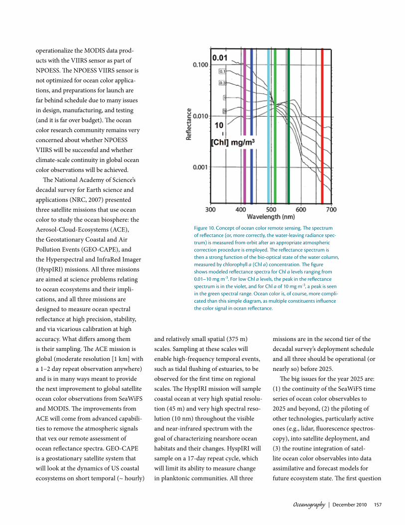
Figure 9 is an example of the current measurement capability of spaceborne sensors, and depicts color-coded chlo-rophyll concentration of the west coast of the United States and Mexico’s Baja California. As Figure 10 shows, the ocean reflectance spectrum is a strong function of the bio-optical state of the water column, here measured by the chlorophyll a concentration (Chl a). For low Chl a levels typical of the blue open ocean, the peak in the reflectance

spectrum is in the violet, while for a Chl a of 10 mg m-3 typical of a coastal phytoplankton bloom, the peak in the reflectance spectrum is found in the green. The science of ocean color is of course more complicated than this simple diagram, as the chlorophyll concentration provides only a first-order description of the ocean color spectrum. Other suspended and dissolved materials in the sea also contribute to ocean color signals (e.g., colored dissolved organic

matter, particle and phytoplankton size spectrum, terrigenous particles, phytoplankton community structure). Resolution of these issues has an impor-tant bearing on the use of ocean color remote sensing for assessing significant ocean biological and biogeochemical processes, such as rates of oceanic carbon sequestration and marine ecosystem status, in routine and accurate ways.

Satellite remote sensing of ocean color began over 20 years ago with the pilot mission, the Coastal Zone Color Scanner (CZCS). CZCS imagery gave biological oceanographers their first opportunities to do research on synoptic and global scales in a routine way. Ocean color images were converted to Chl a concen-tration by employing rather simple atmospheric correction and vicarious calibration procedures. The atmospheric attenuation of the ocean color signal is large and has to be corrected more than the IR signal for SST. More than 10 years after the demise of the CZCS sensor, the Sea-viewing Wide-Field of view Sensor (SeaWiFS) was launched. The SeaWiFS mission has been wildly successful and has provided the research and operations community a decadal view of global ocean biosphere changes. The decadal time series of ocean color observables initiated by SeaWiFS has been supplemented by NASA’s MODIS and ESA’s MEdium Resolution Imaging Spectrometer (MERIS) data sets. The MODIS and MERIS sensors are designed to provide visible through thermal infrared spectral imagery for a wide variety of oceanic, terrestrial, and atmo-spheric applications. As such, they are not optimized for ocean color applica-tions (as SeaWiFS is with its polarization descrambler). Present US plans are to

Figure 9. chlorophyll concentration measured by the SeawiFS (Sea-viewing wide-Field of view Sensor) sensor off the west coast of the united States and mexico in an eight-day composite at 9-km resolution. grayish colors indicate cloud cover, despite the compositing period. Note the filaments and small-scale features.


operationalize the MODIS data prod-ucts with the VIIRS sensor as part of NPOESS. The NPOESS VIIRS sensor is not optimized for ocean color applica-tions, and preparations for launch are far behind schedule due to many issues in design, manufacturing, and testing (and it is far over budget). The ocean color research community remains very concerned about whether NPOESS VIIRS will be successful and whether climate-scale continuity in global ocean color observations will be achieved.

The National Academy of Science’s decadal survey for Earth science and applications (NRC, 2007) presented three satellite missions that use ocean color to study the ocean biosphere: the Aerosol-Cloud-Ecosystems (ACE), the Geostationary Coastal and Air Pollution Events (GEO-CAPE), and the Hyperspectral and InfraRed Imager (HyspIRI) missions. All three missions are aimed at science problems relating to ocean ecosystems and their impli-cations, and all three missions are designed to measure ocean spectral reflectance at high precision, stability, and via vicarious calibration at high accuracy. What differs among them is their sampling. The ACE mission is global (moderate resolution [1 km] with a 1–2 day repeat observation anywhere) and is in many ways meant to provide the next improvement to global satellite ocean color observations from SeaWiFS and MODIS. The improvements from ACE will come from advanced capabili-ties to remove the atmospheric signals that vex our remote assessment of ocean reflectance spectra. GEO-CAPE is a geostationary satellite system that will look at the dynamics of US coastal ecosystems on short temporal (~ hourly)

and relatively small spatial (375 m) scales. Sampling at these scales will enable high-frequency temporal events, such as tidal flushing of estuaries, to be observed for the first time on regional scales. The HyspIRI mission will sample coastal ocean at very high spatial resolu-tion (45 m) and very high spectral reso-lution (10 nm) throughout the visible and near-infrared spectrum with the goal of characterizing nearshore ocean habitats and their changes. HyspIRI will sample on a 17-day repeat cycle, which will limit its ability to measure change in planktonic communities. All three

missions are in the second tier of the decadal survey’s deployment schedule and all three should be operational (or nearly so) before 2025.

The big issues for the year 2025 are: (1) the continuity of the SeaWiFS time series of ocean color observables to 2025 and beyond, (2) the piloting of other technologies, particularly active ones (e.g., lidar, fluorescence spectros-copy), into satellite deployment, and (3) the routine integration of satel-lite ocean color observables into data assimilative and forecast models for future ecosystem state. The first question

Figure 10. concept of ocean color remote sensing. The spectrum of reflectance (or, more correctly, the water-leaving radiance spec-trum) is measured from orbit after an appropriate atmospheric correction procedure is employed. The reflectance spectrum is then a strong function of the bio-optical state of the water column, measured by chlorophyll a (chl a) concentration. The figure shows modeled reflectance spectra for chl a levels ranging from 0.01–10 mg m-3. For low chl a levels, the peak in the reflectance spectrum is in the violet, and for chl a of 10 mg m-3, a peak is seen in the green spectral range. ocean color is, of course, more compli-cated than this simple diagram, as multiple constituents influence the color signal in ocean reflectance.


is particularly vexing. It remains unclear whether VIIRS will result in climate-quality observations of ocean biological processes, and the next US mission is ACE, which will be launched no earlier than 2020 given present budgets. One hope is developing better cooperation with our international space agency partners. ESA’s planned Sentinel-3 will carry an Ocean Land Color Instrument (OLCI) for launch in 2013. NASA’s Preliminary Aerosol, Cloud, Ecosystem (PACE) mission is planned for 2019. In September 2010, the International Ocean Colour Coordinating Group received approval from the Committee for Earth Observation Satellites (CEOS) to develop a “virtual constellation” for ocean color observations. The hope here is that ocean color data records can be merged into uniform climate data records for the global ocean biosphere.

Many issues need to be resolved, both scientific and institutional, before this international collaboration can become a reality. Without it, though, it seems very unlikely that the legacy of high-quality satellite observations that began with the SeaWiFS mission will be continued.

Sea iceIn order to assess the state and mass balance of the polar ice cover, satel-lite observations have proven to be of fundamental importance. The impact of climate change in the polar regions has enhanced the value and need for satellite observations, particularly in the interac-tions of sea ice and ice shelves with the underlying ocean. The increased expo-sure of the polar oceans resulting from sea ice cover retreat directly impacts surface albedo and resulting ocean warming. Sea level is altered by the release of freshwater from the retreating glacier and lowering of the ice sheets. Further, melt from sea ice and ice sheets has an impact on ocean circulation, including upper ocean mixing. Marine ecosystems are shifting in the north from arctic to subarctic regimes with altera-tions in summer warming.

Sea ice observations currently provided include: (1) sea ice extent and large-scale ice motion, both primarily obtained from passive microwave and scatterometer data (Breivik et al., 2010), (2) ice temperature from passive microwave and optical/infrared sensors, (3) fine-scale ice motion from SAR,

which is particularly useful for under-standing the mechanical deformation and redistribution of sea ice, and (4) ice age from combined scatterometer and SAR observations as well as passive micro-wave data. More recently, estimates of ice thickness are derived from freeboard measurements obtained by both lidar and radar altimeters. Sea level is observed by satellite altimeters, and now estimates of changes in water mass are derived from gravity observations. Snow depth on sea ice, an important parameter for examining surface albedo and ice growth rates, is being estimated using passive microwave data. In the coming decade, coordinated and routine observations of these parameters over a broad range of length scales should allow significant progress in monitoring the sea ice cover and understanding the polar oceans.

Recently launched missions of value for polar observations include ESA’s CryoSat-2 (launched in April 2010) and Gravity field and steady-state Ocean Circulation Explorer (GOCE; launched in November 2009); relevant future missions include ESA’s Sentinel-3 that will carry an altimeter similar to those aboard Cryosat and Ice, Cloud, and land Elevation Satellite (ICESat-2). Sentinel-3, under ESA’s GMES program, will carry a radar altimeter similar to the one aboard Cryosat-2, and ICESat-2’s laser altimeter will provide additional measurements of sea ice freeboard with both radar and laser altimeters. SWOT, an imaging interferometer, is capable of providing two-dimensional mapping of ice surface topography. GOCE is a gravity mission that will augment gravity observations by GRACE. The combined observations of freeboard, sea level, and gravity over the polar oceans would enable improved

“New TechNologieS haVe opeNeD The Door To uNForeSeeN ScieNTiFic queSTioNS aND pracTical applicaTioNS, which, iN TurN, haVe guiDeD The NeXT geNeraTioN oF TechNology DeVelopmeNT—a FruiTFul, muTual coupliNg BeTweeN ScieNce aND TechNology.”


determination of ocean circulation and the polar geoid. Regarding SAR obser-vations, there are planned follow-on missions to Envisat and RADARSAT—ESA’s Sentinel-1 and the Canadian Space Agency’s RADARSAT-3. These missions will continue the valuable fine-scale measurements of ice deformation. The NASA decadal survey mission DESDynI is planned for the 2015 –2018 time frame and will be a critical addition. A planned NOAA mission and ESA will continue collecting scatterometer data. Passive microwave observations will continue on several platforms.

Several important observations need to be considered for future missions. An improved capability would be to combine both radar and laser altimeters on a single platform to simultaneously observe the top of the snow (laser) and the top of the ice (radar). These combined observations would improve the value of the freeboard measurements by directly identifying each layer’s height, hence improving sea ice thickness estimates. To fundamentally improve knowledge of sea ice thickness and sea ice mass balance, however, simultaneous observation of the top and bottom sea ice surfaces is required. This observa-tion has been demonstrated using a low-frequency wideband penetrating radar. The direct observation of sea ice thickness would remove basic assump-tions needed to estimate thickness from freeboard, including ice density and the relation of surface topography to bottom topography. Another observation of high interest would be sea surface salinity to address freshwater fluxes relating to river inflow into the Arctic, particularly, and also ice and snow melt, a key parameter that affects ocean mixing and circulation.

gr aViT yTime-varying gravimetric data from space measure mass changes in Earth. On seasonal to interannual time scales, mass changes are dominated by water exchanges among locations and reser-voirs (ocean, land, cryosphere, atmo-sphere). In addition, these changes are affected by tectonic displacements, such as the Sumatra earthquake of 2004, or postglacial rebound.

The GRACE mission, launched in 2002, has proven revolutionary, measuring the mass loss from Greenland and Antarctica (e.g., Velicogna, 2009), an elusive goal before GRACE, and more recently from Alaska glaciers. GRACE is also capable of measuring hydrologic and oceanographic quantities (e.g., Chambers and Willis, 2009). In physical oceanographic studies, GRACE is being used to close the budget that distinguishes the components of sea level rise (measured by radar altimetry) due to thermal expansion and to mass addition due to ice melting. In addition, gravity changes over the ocean are a proxy for ocean bottom pressure, whose time-varying gradient yields the time-varying component of deep geostrophic flow.

GRACE will likely continue until 2012–2013. A GRACE “gap-filling” mission is now planned for launch in 2015. The decadal survey (NRC, 2007) has placed GRACE II in the 2016–2020 time frame. The gap-filling mission will likely use the same satellite configura-tion and same microwave link between the two satellites as GRACE does, plus an experimental laser link that promises increased accuracy. A third mission, to be launched in the 2020 time frame, is under discussion, using satellite combinations other than GRACE’s

“two-satellites-colinear” configura-tion. These configurations include “four-satellite-cartwheel” and two “two-satellite-colinear,” but in different repeat orbits. Both of these configura-tions improve retrieval of shorter-period signals and reduce aliasing errors due to short-period hydrologic and oceanic mass movements. Because of the interest in many space-faring countries to contribute to measuring time-varying gravity from space, it is quite likely that combinations of these gravity pairs will exist in 2025, yielding increased accuracy and resolution. In addition to these improvements, the current GPS constellation will have been augmented by the European Galileo and improved Russian Global Navigation Satellite System (GLONASS), jointly known as the Global Navigation Satellite Systems (GNSS), which will provide much more continuous coverage, and thus more accurate and frequent satellite positions, and allow for added accuracy in the retrieval of low-degree, long-wavelength gravity coefficients.

oceaN waVeSWind waves, whether generated by local or far-away winds, have important practical consequences in navigation, offshore operations, recreation, and many other areas. Swail et al. (2010) summarize observational requirements for wave models, climate studies, and a host of applications: “(i) significant wave height; (ii) dominant wave direction; (iii) wave period; (iv) 1-D frequency spectral wave energy density; and (v) 2-D frequency-direction spectral wave energy density. Also important are observations of individual wave components (sea/swell). In the study of


ocean waves, high quality wind observa-tions, both in-situ and remote, are often as important as the wave observations themselves.” Of these needs, a subset can be observed from space. The same satellite radar altimeters as those used for SSH have provided significant wave height continuously for over two decades (starting with the Geodetic and Earth Orbiting Satellite 3 [GEOS-3] and continuing at present with Envisat and Jason-2). SARs yield directional and wavenumber information (Figure 11; Holt, 2004; Vachon et al., 2004). The

Canadian RADARSAT-1 and -2, European ERS-1 and -2, Japanese ALOS/PALSAR (Phased Array type L-band Synthetic Aperture Radar), German Terrasar-X, and European Envisat ASAR have all flown, or are still in opera-tion, providing sea state information with 25-m resolutions over long strips about 100-km wide, or 100-m resolu-tion over 500-km-wide area strips. Numerical wave models require marine surface wind vector data, which are constrained by the scatterometers and SARs discussed above.

All improvements to the coverage and resolution of nadir radar altimeters and SARs will help provide the detailed wave information needed to model and use wind wave information.

TechNological aDVaNceSThe kind of technology advances that will enable the improvements in ocean measurements from space described above include:• Miniaturized, more efficient radar

components to reduce mass/power needs of radar electronics

• Efficient, high-power transmitters at shorter wavelengths (especially Ku- and Ka-band)

• Increased onboard processing and/or downlink capability, allowing data acquisition at higher spatial and temporal resolution

• Larger deployable antennas in the 6–12 m range, particularly employed in a conical scan mode, enabling higher-resolution radiometry and scatterometry

• A scanning interferometer pair of antennas, rotating through an azimuth scan of 360° to provide along-track interferometry measurements of surface currents at high resolution

• Precision formation flying, to enable bistatic wide-swath SSH measure-ments from two platforms flying in formation, and gravity measurements from multiple platforms

• Laser interferometry to improve the accuracy of gravity measurements from future GRACE-like missions

• Wide-field-of-view imaging spec-trometers with improved stability and signal-to-noise ratio, and atmospheric correction capabilities, enabling global ocean biosphere measurements

Figure 11. raDarSaT-1 image taken November 22, 2001, at 14:24 uTc showing ocean surface waves refracting along point reyes Beach and around point reyes (the leftmost point), into Drake’s Bay, point reyes National Seashore, ca, uSa. The image covers 26 km x 26 km and was processed at the alaska Satellite Facility. a bright ship and its wake are shown turning off point reyes. Figure © 2001 Canadian Space Agency


at moderate resolution (~ 1 km) on a daily basis and fine resolution (60 m) on a synoptic basis

• Deployment of ocean color imagers on geostationary platforms to sample the highly dynamic processes of coastal ecosystems

• Spaceborne implementation of active remote sensing of biochemical constituents of the ocean, including fluorescence spectroscopy instru-ments (UV/visible) and lasers at the blue end of the visible spectrum to measure mixed-layer depth, as input to biochemical models

• Increased computational power to allow more complex coupled models to be run at higher resolutions, with data assimilation

ackNowleDgemeNTSThe work described in this paper was, in part, carried out at the Jet Propulsion Laboratory, California Institute of Technology, under contract with the National Aeronautics and Space Administration.

reFereNceSBreivik, L., T. Carrieres, S. Eastwood, A. Fleming,

F. Girard-Ardhuin, J. Karvonen, R. Kwok, W.N. Meier, M. Mäkynen, L.T. Pedersen, and others. 2010. Remote sensing of sea ice. In Proceedings of OceanObs’09: Sustained Ocean Observations and Information for Society (Vol. 2). Venice, Italy, September 21–25, 2009, J. Hall, D.E. Harrison, and D. Stammer, eds, ESA Publication WPP-306. Available online at: http://www.oceanobs09.net/blog/?p=63 (accessed September 30, 2010).

Chambers, D.P., and J.K. Willis. 2009. Low-frequency exchange of mass between ocean basins. Journal of Geophysical Research 114, C11008, doi:10.1029/2009JC005518.

DiGiacomo, P.M., and B. Holt. 2001. Satellite observations of small coastal ocean eddies in the Southern California Bight. Journal of Geophysical Research 106(C10):22,521–22,544.

Donelan, M.A., B.K. Haus, N. Reul, W.J. Plant, M. Stiassnie, H.C. Graber, O.B. Brown, and E.S. Saltzman. 2004. On the limiting aerody-namic roughness of the ocean in very strong winds. Geophysical Research Letters 31, L18306, doi:10.1029/2004GL019460.

Fu, L., D. Alsdorf, E. Rodriguez, R. Morrow, N. Mognard, J. Lambin, P. Vaze, and T. Lafon. 2010. The SWOT (Surface Water and Ocean Topography) mission. In Proceedings of OceanObs’09: Sustained Ocean Observations and Information for Society (Vol. 2). Venice, Italy, September 21–25, 2009, J. Hall, D.E. Harrison, and D. Stammer, eds, ESA Publication WPP-306. Available online at: http://www.oceanobs09.net/blog/?p=81 (accessed September 30, 2010).

Holt, B. 2004. SAR imaging of the ocean surface. Pp. 25–79 in Synthetic Aperture Radar (SAR) Marine User’s Manual. C.R. Jackson and J.R. Apel, eds, NOAA NESDIS Office of Research and Applications, Washington, DC. Available online at http://www.sarusersmanual.com (accessed September 30, 2010).

Lagerloef, G., J. Boutin, Y. Chao, T. Delcroix, J. Font, P. Niiler, N. Reul, S. Riser, R. Schmitt, D. Stammer, and F. Wentz. 2010. Resolving the global surface salinity field and variations by blending satellite and in situ observations. In Proceedings of OceanObs’09: Sustained Ocean Observations and Information for Society (Vol. 2). Venice, Italy, September 21–25, 2009, J. Hall, D.E. Harrison, and D. Stammer, eds, ESA Publication WPP-306. Available online at: http://www.oceanobs09.net/blog/?p=567 (accessed September 30, 2010).

Lee, T. 2004. Decadal weakening of the shallow overturning circulation in the South Indian Ocean. Geophysical Research Letters 31, L18305, doi:10.1029/2004GL020884.

Meissner, T., and F.J. Wentz. 2009. Wind-vector retrievals under rain with passive satellite microwave radiometers. IEEE Transactions on Geoscience and Remote Sensing 47(9):3,065–3,083.

Monaldo, F.M., D.R. Thompson, W.G. Pichel, and P.A. Clemente-Colòn. 2004. Systematic compar-ison of QuikSCAT and SAR ocean surface wind speeds. IEEE Transactions on Geoscience and Remote Sensing 42(2):283–291.

Monaldo, F.M., D.R. Thompson, R.C. Beal, W.G. Pichel, and P. Clemente-Colòn. 2001. Comparison of SAR-derived wind speed with model predictions and ocean buoy measure-ments. IEEE Transactions on Geoscience and Remote Sensing 39:2,587–2,600.

Monaldo F.M., D.R. Thompson, W.G. Pichel, and P. Clemente-Colon. 2004. A systematic compar-ison of QuikSCAT and SAR ocean surface wind speeds. IEEE Transactions on Geoscience and Remote Sensing 42(2):283–291, doi:10.1109/TGRS.2003.817213 .

NRC (National Research Council). 2007. Earth Science and Applications from Space: National Imperatives for the Next Decade and Beyond. Committee on Earth Science and Applications from Space: A Community Assessment and Strategy for the Future, National Academies Press, Washington, DC, 456 pp.

Swail, V., R.E. Jensem, B. Lee, J. Turton, J. Thomas, S. Gulev, M. Yelland, P. Etala, D. Meldrum, W. Birkmeier, W. Burnett, and G. Warren. 2010. Wave measurements, needs and develop-ments for the next decade. In Proceedings of OceanObs’09: Sustained Ocean Observations and Information for Society (Vol. 2). Venice, Italy, September 21–25, 2009, J. Hall, D.E. Harrison, and D. Stammer, eds, ESA Publication WPP-306. Available online at: http://www.oceanobs09.net/blog/?p=274 (accessed September 30, 2010).

Thompson, D.R., F. Monaldo, S. Iris, and H.C. Graber. 2005. Can synthetic aperture radars be used to estimate hurricane force winds? Geophysical Research Letters 32, L22801, doi:10.1029/2005GL023992.

Vachon, P.W., F.M. Monaldo, B. Holt, and S. Lehner. 2004. Ocean surface waves and spectra. Pp. 139–169 in Synthetic Aperture Radar (SAR) Marine User’s Manual. C.R. Jackson and J.R. Apel, eds, NOAA NESDIS Office of Research and Applications, Washington, DC. Available online at: http://www.sarusersmanual.com (accessed September 30, 2010).

Velicogna, I. 2009. Increasing rates of ice mass loss from the Greenland and Antarctic ice sheets revealed by GRACE. Geophysical Research Letters 36, L19503, doi:10.1029/2009GL040222.

ocean measurements from space in 2025 - ron kwok - nasa

Documents