ocean modelling - geophysical fluid dynamics … mesoscale eddies with residual and eulerian...

Ocean Modelling 23 (2008) 1–12

Contents lists available at ScienceDirect

Ocean Modelling

journal homepage: www.elsevier .com/ locate/ocemod

Parameterizing mesoscale eddies with residual and Eulerian schemes,and a comparison with eddy-permitting models

Rongrong Zhao, Geoffrey Vallis *

Atmospheric and Oceanic Science Program, Princeton University, Princeton, NJ 08544, USA

a r t i c l e i n f o

Article history:Received 9 May 2007Received in revised form 11 February 2008Accepted 12 February 2008Available online 5 March 2008

1463-5003/$ - see front matter � 2008 Elsevier Ltd. Adoi:10.1016/j.ocemod.2008.02.005

* Corresponding author.E-mail addresses: [email protected] (R.

(G. Vallis).

a b s t r a c t

In this paper we explore and test certain parameterization schemes that aim to represent the effects ofunresolved mesoscale eddies on the larger-scale flow. In particular, we examine a scheme based onthe residual or transformed Eulerian mean formulation of the equations, in which the eddies are param-eterized by a large vertical viscosity in the momentum equations, with no skew flux parameterizationappearing in the tracer (e.g., temperature or salinity) evolution equations, although terms that parame-terize diffusion along isopycnal surfaces remain.The residual scheme is compared both to a conventional parameterization that uses a skew diffusion (orequivalently advection by a skew velocity), and to eddy-permitting calculations. Although in principlealmost equivalent to certain forms of skew flux schemes, the residual formulation is found to have certainpractical advantages over the conventional scheme in some circumstances, and in particular near theupper boundary where conventional schemes are sensitive to the choice of tapering but the residualscheme is less so. The residual scheme also enables the horizontal viscosity – which is mainly appliedto maintain model stability – to be reduced. Finally, the residual scheme is somewhat easier to implement,and the tracer transport is easier to interpret. On the other hand, the residual scheme gives, at least for-mally, a transformed velocity, not the Eulerian velocity and will not be appropriate in all circumstances.

� 2008 Elsevier Ltd. All rights reserved.

1. Introduction

Mesoscale eddies in the ocean have a scale of tens to hundredsof kilometers, and consequently their effects are not explicitly ac-counted for in coarse resolution ocean climate models that cur-rently may have a grid spacing of over 1�. It is often thought thata resolution closer to 1/6�, probably higher in some regions ofthe ocean, is necessarily to account, even imperfectly, for their ef-fects. Now, and relatedly, observations indicate that in the oceaninterior diapycnal diffusion is appropriately small (e.g., Ledwellet al., 1998, Toole et al., 1994) and that the motion is predomi-nantly adiabatic; that is, advective effects dominate diffusive ef-fects. However, in the top and (to a lessor degree) bottomboundary layers the flow may be diabatic, and both advectiveand diffusive effects are important. Thus, it is commonly thoughtthat any parameterization of mesoscale eddies should be predom-inantly adiabatic in the ocean interior, transitioning in some way toa diabatic scheme in the mixed layer.

A widely used eddy parameterization scheme for current oceanmodels was developed by Gent and McWilliams (1990) and Gentet al. (1995) (hereafter GM). The GM scheme may be formulated

ll rights reserved.

Zhao), [email protected]

either as an eddy advection term or equivalently as eddy skew fluxusing an anti-symmetric diffusion tensor, as described by Griffies(1998). In either case it is applied in the tracer equations, that isin the evolution equations for temperature, salinity and any pas-sive tracers that may be present. The GM scheme of itself is adia-batic, and as such is appropriate for the ocean interior. It hasbeen a very successful parameterization, although its implementa-tion in ocean models is not without its problems. In particular, dia-batic effects in the upper mixed layer are often incorporated byreducing the slope along which the parameterized tracer flux oc-curs as the surface is approached. That is, in the adiabatic flow inte-rior the flux is parallel to the contours, but as the surface isapproached the flux is allowed to cross-isopycnal surfaces. Climatemodels are found to be rather sensitive to the precise way in whichthis is done. For instance, Gough and Welch (1994) found oceanmodels are sensitive to the tapering constants such as maximumallowable isopycnal slope, and in more recent simulations of Gna-nadesikan et al. (2007) (using the GDFL MOM model), it is alsoshown that an increase on Smax (a number for onset of slope taper-ing in GM) makes a distinctive differences in such as the verticalstructure of temperature distribution, the ventilation of southernocean, and mixed layer depth.

In conjunction with the advective GM scheme, mesoscale eddyparameterizations normally include, following Redi (1982), a diffu-sion of tracers (both active and passive) along neutral surfaces.

mailto:[email protected]

mailto:[email protected]

http://www.sciencedirect.com/science/journal/14635003

http://www.elsevier.com/locate/ocemod

2 R. Zhao, G. Vallis / Ocean Modelling 23 (2008) 1–12

Such diffusion must also be tapered near the surface in order thatthe flux be horizontal. If there is no salinity, and an equation ofstate of the form q ¼ qðhÞ, then there is evidently no diffusion oftemperature along isopycnal surfaces (this is the case in the simu-lations we perform), although the scheme will give a horizontal,and diabatic, diffusion of buoyancy near the surface.

An alternative to the conventional GM scheme is to recast theequations in residual form, using the transformed Eulerian mean.(See Andrews et al. (1987) or Vallis (2006) for general background,Greatbatch and Lamb (1990), Greatbatch and Li, 1990 and Great-batch (1998) for theoretical analysis and discussion in an oceancontext, Wardle and Marshall (2000) and Ferreira and Marshall(2006) for applications in an ocean model, and Holloway (1997)for a discussion of the relation of thickness diffusion to eddymomentum effects.) In the residual scheme, the eddy buoyancyterms are transformed away from the buoyancy equation, and re-appear in the momentum equation where they combine with theeddy momentum fluxes to give potential vorticity fluxes, poten-tially with ensuing conceptual and computational simplifications.No eddy advection terms are needed in the tracer equations,although a Redi diffusion for each tracer must still be calculated.Also, the residual formulation does, at least formally, predict theresidual velocities and not the local Eulerian velocities, whichmay be disadvantageous in some circumstances. Although on theone hand such a recasting may be regarded merely a formal trans-formation of the equations, the practical differences in implement-ing a parameterization scheme may be significant. Further, giventhe general uncertainty of any parameterization scheme, havinga mesoscale parameterization in the momentum equation is atleast as a priori justifiable as having one in the thermodynamicequation.

2. Eddy parameterizations

2.1. Tracer equation

The governing equation for a tracer, b, may be written

o�botþ �v � r�bþr � v0b0 ¼ S þ D ð2:1Þ

We will regard b as buoyancy, and for simplicity salinity will beabsent from our considerations, a restriction that is fairly easilyrelaxed. In (2.1) we have decomposed the velocity in the standardway into two parts: a resolved Eulerian mean velocity �v, and anunresolved perturbation v0, or sub-grid scale (SGS) velocity. Theoverbar may be regarded as a kind of low-pass filter, acting overa coarse-grid cell that is fixed in space, with the primed variablesrepresenting motions that are unresolved on the coarse-grid. TheSGS motions affect the large-scale motion through the termr � v0b0, and need to be parameterized in the coarse-grid model.(It may be argued that model variables should be naturally inter-preted as thickness-weighted isopycnal averages, and thickness-weighting naturally leads to a residual form of the equations,but we do not pursue this line of argument here.) On the right-hand side of (2.1), S is any external heating and cooling process,which are important mainly near the ocean surface. The term Drepresents vertical and horizontal diffusive processes on the fine-scale and molecular processes, but not on the mesoscale we seekto parameterize; that is, we assume that it is meaningful to sepa-rate the parameterizations for the mesoscale and the fine scale.The term includes a vertical diffusion term, ozðjvozbÞ, that repre-sents the real physical process of internal wave breaking leadingto a diapycnal diffusion; jv has a measurable, albeit small value,meaning that over most of the ocean interior the vertical diffusiondoes not enter the leading order balance of (2.1). Any horizontal

diffusion that is included in D, jhr2hb for example, would be less

physical, being included in ocean models mainly for numericalreasons with the value for jh being dependent on the modelresolution.

Let us decompose the eddy flux, F ¼ v0b0, into two parts: onethat is diapycnal (i.e., across contours of �b) and denoted F?, andone that is isopycnal (i.e., aligned along contours of �b) and denotedFk:

v0b0 ¼ F? þ Fk ¼v0b0 � r�b

j r�bj2r�b� v0b0 � r�b

j r�bj2�r�b ð2:2Þ

This is a vector identity, as may be verified by expanding the vectortriple product in the last term on the right-hand side. (The gradientoperator in this expression is three-dimensional; the horizontaloperator will be denoted rh.) The diapycnal component of eddybuoyancy flux F? is important primarily in the mixed layer. Thealong isopycnal flux Fk, important in both ocean interior and oceanboundary, is the main topic of current work. Eden et al. (2007) dis-cuss such eddy flux decompositions in more detail.) Taking thedivergence of the along isopycnal term in (2.2) and applying a vec-tor identity gives

r � Fk ¼ �r �v0b0 � r�b

j r�bj2�r�b

( )¼ � r� v0b0 � r�b

j r�bj2

( )� r�b ð2:3Þ

If we define an eddy streamfunction and eddy velocity as

W ¼ � v0b0 � r�b

j r�bj2; v� ¼ r �W; ð2:4a;bÞ

then we may write (2.1) as

o�botþ �v � r�bþ v� � r�b ¼ r � F? þ S þ D: ð2:5Þ

The effect of Fk is evidently equivalent to an advection processby the eddy velocity v�, and so is manifestly adiabatic in that itdoes not change the census of �b. If j bz j�j rh

�b j, as is generallythe case away from boundaries, then the eddy streamfunction is gi-ven by (see Appendix A for more detail)

W � �iv0b0

�bzþ j

u0b0�bz

ð2:6Þ

and this is the form we shall mostly be concerned with.The diapycnal flux divergence term r � F? is often considered to

be negligible in ocean interior and only important near oceanboundaries, and eddy parameterizations for tracers are often mod-elled using an advective scheme (using the eddy velocity v�) for theinterior ocean domain and a diffusive scheme for ocean boundarylayers.

2.2. The residual momentum equation

If a residual velocity ~v is defined as the sum of �v and v�, that is~v ¼ v þ v� (2.5) can be written as:

o�botþ ~v � r�b ¼ r � F? þ S þ D ð2:7Þ

If we are to use (2.7) to simulate tracers then we need an equationfor the residual velocity, and we will derive this in an informal way.In a geostrophic flow, the main balance for horizontal momentum isbetween Coriolis force and horizontal pressure gradient:

f � u � �r/ ð2:8Þ

where f ¼ f k. We write this in residual form by adding an eddyvelocity term (A3) into both sides of the equation, giving

R. Zhao, G. Vallis / Ocean Modelling 23 (2008) 1–12 3

f � ~u � �r/þ f � u� ð2:9Þ

� �r/þ f � �ozðu0b0=oz�bÞ

�ozðv0b0=oz�bÞ

!ð2:10Þ

¼ �r/þ fo

ozðv0b0=oz

�bÞ�ðu0b0=oz

�bÞ

!ð2:11Þ

To parameterize u0b0 and v0b0 in the ocean interior we use downgradient eddy fluxes

u0b0 ¼ �j�bx; v0b0 ¼ �j�by: ð2:12Þ

Using this and the thermal wind relation,

�bx � f �vz;�by � �f �uz; ð2:13a;bÞ

Eq. (2.11) becomes

f � ~u � �r/þ o

ozjf 2 oz �u

oz�b

� �: ð2:14Þ

If we define eddy viscosity me as

me � jf 2

N2 ¼ jf 2

�ðg=q0Þoqz=oq ; ð2:15Þ

then, restoring advection (2.14) becomes

D�uDtþ f � ~u ¼ �r/þ osm

ozþ o

ozme

o�uoz

� �: ð2:16Þ

where sm is the mechanical stress from the wind and viscosity, aswould also appear in the non-transformed equations. A similar formwas previously obtained by Greatbatch and Lamb (1990). To get themomentum equation for residual velocity, an approximation ismade on (2.16) to replace �u with the residual velocity ~u in theadvection term and friction term. This is a good approximation atlow Rossby number: u� is small comparing to �u at least in the oceaninterior; the approximation is on advection and friction terms, sothe dominant geostrophic balance is not affected; and the uncer-tainty in the parameterization itself certainly warrants an imple-mentation of an approximated equation of residual velocity. Thusthe residual form momentum equation for our simulations is

D~uDtþ f � ~u ¼ �r/þ osm

ozþ ose

ozð2:17aÞ

where the eddy stress se is given by

se ¼ meo~uoz: ð2:17bÞ

except near the ocean surface as discussed in the next section. Theeddy velocity of the residual scheme, u�rs, satisfies

f � u�rs ¼o

ozme

o~uoz

� �: ð2:18Þ

A similar evolution equation was used by Ferreira and Marshall(2006). The parameterization embodied by (2.17) is manifestly adi-abatic, for it affects only the momentum equation. The parameter-ization goes to zero at the equator, where f ¼ 0, if j remainsfinite. However, our derivation is valid only for small Rossby num-bers and should not be expected to work at very low latitudes. Thenature of the eddy field is also different at the equator. For both ofthese reasons, then, the parameterization should be regarded asapplying to mid-latitude eddies only.

2.3. The diabatic surface layer

As the top ocean boundary is approached, eddy fluxes becomealigned more horizontally, whereas isopycnals become steeperdue to the active vertical mixing in the mixed layer. As a conse-quence eddy motions are cross-isopycnal and diabatic. Therefore,

the above arguments for an adiabatic, advective parameterizationare no longer suitable in this region [as noted by, among others,Treguier et al. (1997); additional discussion is to be found in Edenet al. (2007)]. A truly satisfactory theoretical framework for thebehavior of eddy fluxes as the surface is approached remains tobe developed, and current schemes have been designed to satisfysimple physical restrictions, such as forcing the eddy velocity tobe along-surface in the surface layer. In addition, an upper boundon the magnitude on the diffusivity must be set: in the ocean inte-rior the isopycnal slope is small and it may sensibly be used todetermine the magnitude of an eddy diffusivity. However, in themixed layer isopycnal slopes are large — potentially infinite —and the eddy diffusivity of the conventional GM scheme, and theeddy viscosity of (2.15), must be capped in order to maintain mod-el stability.

Accordingly, eddy parameterizations may have two aspects: (i)as needed, numerical limits on parameters are set to prevent themodel from going unstable; and (ii) the eddy velocity is prescribedto be horizontal, with no eddy flux across the ocean surface. Often,treatments will force the eddy velocity to be constant throughoutsurface diabatic layer of some specified thickness. One exampleis the slope tapering for GM scheme which has been implementedin present GFDL/MOM Griffies (1998), where the eddy streamfunction is linearly tapered off to produce a constant eddy velocityacross the surface diabatic layer. This additional treatment is inpart supported by some earlier analysis based on eddy-resolvingsimulation of Kuo et al. (2005) which shows the horizontal compo-nent of mesoscale eddy fluxes are nearly constant throughout thesurface diabatic layer.

The boundary condition on the mechanical stress at the top ofthe ocean is obtained by setting the momentum flux equal to thewind stress at the top of the ocean; that is

smðz ¼ 0Þ ¼ sw; ð2:19Þ

where sw is the given wind stress. The simplest treatment of theupper boundary condition on the eddy stress in the residual frame-work is simply to set the eddy stress equal to zero at the top, withno explicit tapering, so that meoz ~u ¼ 0 at z ¼ 0. The wind stress isadded as a separate term at the upper boundary. (However, this isnot wholly satisfactory from a physical standpoint because onemight wish to include the wind stress at the upper boundary byway of a boundary condition of the form moz ~u ¼ sm, where m is a con-stant, but this is not possible if it is deemed that the eddy stressshould be zero at the top. But if we were to choose moz ~u ¼ sm, thenthe eddy stress would not necessarily integrate to zero over the do-main, as required for momentum conservation.) A similar conditionis applied at the bottom of the ocean, and with the mechanicalstress sm there being given by a linear drag, chosen to be rather lar-ger than the standard value to partially compensate for choice of aflat bottom. In the upper ocean we have also used somewhat moreelaborate two-step scheme, as follows. The first step is to cap me [de-fined in (2.15)] by a constant mmax for very weakly stratified regionswhere N2 is small and me is large. Thus, we set

mrse ¼minðme; mmaxÞ: ð2:20Þ

Now mrse is the eddy viscosity that the model actually uses. Given

mrse , an intermediate eddy velocity u�inter may be calculated that

satisfies

f � u�inter ¼o

ozmrs

eo~uoz

� �; ð2:21Þ

along with the boundary condition (2.19). No additional treatmentis needed to force the eddy fluxes to be along-surface at z ¼ 0.

The second step of the treatment is to force the eddy velocity tobe constant in the top layer of specified thickness Ds, by setting se

to be a linear function of z, chosen such that the eddy stress goes to


zero at the ocean top (so that the total stress is given by the wind).[Similar requirements are made by Ferreira and Marshall (2006)and Ferrari and McWilliams (pers. comm).] In our simulations weset Ds to be constant, but other potentially more physical choicesare of course possible (for example, choosing the depth to be equalto a deformation radius multiplied by the isopycnal slope). Thus,the final eddy stress is given by

seðzÞ ¼mrs

e o~u=oz for z 6 �Ds

cmrse o~u=ozj�Ds

for z P �Ds

(ð2:22Þ

where c, a tapering coefficient, goes from zero at the surface to unityat z ¼ �Ds. The eddy velocity (if needed) then follows fromf � u�rs ¼ ose=oz, and in the upper ocean the eddy velocity has, byconstruction, no shear. A schematic of this treatment is given inthe left panel of Fig. 1, although the eddy velocity is not guaranteedto be continuous at z ¼ �Ds. The two-step tapering generally resultsin a three-layer eddy velocity: an interior region (z < �Ds andme < mmax); an intermediate region (z < �Ds and me P mmax); and asurface region ðz > �DsÞ. We may note that if the vertical eddy vis-cosity is large, as it will be from (2.15) if the stratification is weak,then the residual velocity will in any case be nearly constant withheight, so that forcing it to be constant may have little additionaleffect. At the ocean bottom a similar scheme may be employed.However, eddy effects are weak there and we do not taper the eddystresses.

It is informative to compare this scheme to the slope taperingused for GM parameterization in current GFDL ocean model. Inthe latter scheme, the local isopycnal slope S is used to calculateeddy streamfunction. As the top of ocean is approached, isopycnalsbecome steep and S needs to be capped by a constant Smax to pre-vent the eddy streamfunction going to infinity. And in the regionswhere S is capped, the eddy flux is forced to be constant

WxgmðzÞ ¼

jgmSy for z 6 �HjgmSmaxz=H for z P �H

(ð2:23Þ

Here Wxgm is the zonal component of GM eddy streamfunction, and

its vertical derivative results in meridional eddy velocity. Sy is theisopycnal slope in y� z plane, and H is the depth where Sy justturned to be greater than Smax. As a result, the GM eddy velocity is

v�gm ¼oðjgmSyÞ=oz for z 6 �HjgmSmax=H for z P �H

(ð2:24Þ

This treatment thus establishes a layer of depth H for eddy velocityv�gm to be constant. The right panel of Fig. 1 plots a typical eddyvelocity resulted from this slope tapering: it often produces a verysharp shear in v�gm between ocean interior and surface diabaticlayer. This sharp shear is somewhat unphysical and could overeffectively flatten local isopycnals, therefore falsely alter the local

Ds

H

ygm Sz

v*

HSv gm

max*

constv rs*

z

u

zfv rs

~max*

z

u

zfv ers

~1*

z

Fig. 1. Vertical profile of eddy velocity resulted from tapering treatments. The 2-step tapering (left) of residual scheme results in a much smoother transition foreddy velocity from ocean interior to upper boundary, as comparing to slope tape-ring (right) of GM scheme in current GFDL climate model.

stratification. As noted in the introduction, previous studies alsofound that model results are sensitive to the variation of taperingparameter Smax, which is mostly chosen for numerical reasons andin a somewhat arbitrary way. In our simulations, we found thatthe residual scheme tapering, composed of two-step treatment of(2.20) and (2.22), produces a somewhat smoother transition towardtop boundary, and numerical stability is also improved. More re-sults about this will be presented in Section 4.4.

Finally, in some simulations the horizontal mixing of buoyancyis increased in the mixed layer, via the addition of a termrh � ðjmlrhTÞ, with jml an enhanced diffusivity. This term repre-sents the enhanced diabatic mixing that is expected to occur inthe oceanic mixed layer.

3. The model

We have tested the parameterization schemes described abovein a primitive equation model in an idealized channel plus basindomain, as illustrated schematically in Fig. 2. The whole domainis in southern hemisphere extending from 20 �S to 50 �S, wherethe channel region is 24� in zonal extent, and 10� meridional; thegyre region is 20� zonal and 20� meridional. The domain is3000 m deep with flat bottom. The model is both wind and buoy-ancy-driven; the wind distribution is also given in Fig. 2. Thermo-dynamic forcing is via a sea surface restoring temperature that isdecreasing linearly toward the south, with 4 �C at the southernend and 18 �C at the northern end; for simplicity there is no salt.

All simulations in present work are run with GFDL/MOM4,which is z-coordinate model with hydrostatic and Boussinesqapproximations. The model equations of motion are

ouotþ ðv � rÞuþ f � u ¼ �1

q0rhpþ os0m

ozþrh � ðmhrhuÞ ð3:1Þ

PðzÞ ¼ Pa þ gZ g

zdz0q ð3:2Þ

gt ¼ r � U ð3:3Þq ¼ q0 � aðT � T0Þ ð3:4ÞoTotþ ðv � rÞT ¼ o

ozjz

oToz

� �þr � ðjGMrTÞ þ ST ð3:5Þ

Here, u is the two-dimensional horizontal velocity, v is the three-dimensional velocity, U is the vertically integrated horizontal veloc-ity (the ‘barotropic’ velocity), p is pressure, g is surface height, q isdensity, and T is potential temperature. The stress in (3.1) is givenby s ¼ mzozu; the boundary conditions are that at the top of themodel the stress is proportional the surface wind (taken as purely

Fig. 2. Idealized channel model and wind stress distribution.


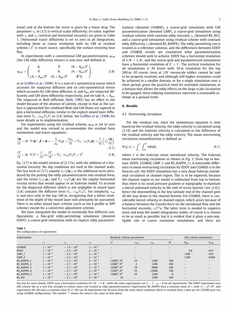
zonal) and at the bottom the stress is given by a linear drag. Theparameter jz in (3.5) is vertical scalar diffusivity; its value, togetherwith mz and mh (vertical and horizontal viscosity) are given in Table1. (Horizontal tracer diffusivity is set to zero in all integrations,including those at coarse resolution with no GM or residualscheme.) ST is tracer source, specifically the surface restoring heatflux.

In experiments with a conventional GM parameterization, jGM

(the GM eddy diffusivity tensor) is non-zero and defined as

jGM ¼AI 0 ðAI � AgmÞSx

0 AI ðAI � AgmÞSy

ðAI þ AgmÞSx ðAI þ AgmÞSy S2AI

0B@

1CA; ð3:6Þ

as in Griffies et al. (1998). It is a sum of a symmetrical tensor whichaccounts for isopycnal diffusion and an anti-symmetrical tensorwhich accounts for GM skew diffusion. AI and Agm are isopycnal dif-fusivity and GM skew diffusivity respectively, and we take AI ¼ Agm.The isopycnal or Redi diffusion (Redi, 1982) has no effect in ourmodel because of the absence of salinity, except in that as the sur-face is approached the combined Redi and GM fluxes are tapered togive a horizontal diffusion, similar to the explicit mixed layer diffu-sion term rh � ðjmlrhTÞ in (3.8) below. See Griffies et al. (1998) formore details as to implementation.

For experiments using the residual scheme, jGM is set to zeroand the model was revised to accommodate the residual formmomentum and tracer equations:

o~uotþ ð~v � rÞ~uþ f � ~u ¼ � 1

q0rhpþ osm

ozþrh � ðmhrh ~uÞ þ o

ozmrs

eo~uoz

� �ð3:7Þ

oTotþ ð~v � rÞT ¼ o

ozðjz

oTotÞ þ rh � ðjmlrhTÞ þ ST ð3:8Þ

Eq. (3.7) is the model version of (2.17a), with the addition of a hor-izontal viscosity. No slip conditions are used at the channel walls.The last term in (3.7), namely ozðmrs

e~uzÞ, is the additional term intro-

duced by the putting the eddy parameterization into residual form,and the terms ozðmz ~uzÞ and rh � ðmhrh ~uÞ are the regular horizontalviscous terms that would appear in an Eulerian model. To accountfor the diapycnal diffusion which is not negligible in mixed layer(3.8) contains the diffusive term rh � ðjmlrhTÞ. For simplicity, jml

is non-zero only in the top 100 m, recognizing that a better treat-ment of the depth of the mixed layer will ultimately be warranted.There is no other mixed layer scheme (such as the k-profile or KPPscheme) except for a convective adjustment scheme.

We have integrated the model in essentially five different con-figurations: a fine-grid eddy-permitting simulation (denotedEDDY), a coarse-grid simulation with no explicit eddy parameter-

Table 1The configurations of experiments

Experiments Residual

mz mh jz mrse

COARSE 1� 10�4 3:5� 104 2� 10�5 –EDDY 1� 10�4 3:5� 104 2� 10�5 –GMP_1 1� 10�4 3:5� 104 2� 10�5 –GMP_2 1� 10�4 3:5� 104 2� 10�5 –RS_KAPPA_1 1� 10�4 2:7� 104 2� 10�5 1200f 2=NRS_KAPPA_2 1� 10�4 2:7� 104 2� 10�5 1200f 2=NRS_KAPPA_3 1� 10�4 2:7� 104 2� 10�5 1200f 2=NRS_KAPPA_4 1� 10�4 2:7� 104 2� 10�5 1200f 2=NRS_KAPPA_5 1� 10�4 2:7� 104 2� 10�5 1200f 2=NRS_NU 1� 10�4 2:7� 104 2� 10�5 1

See text for more details. EDDY uses a horizontal resolution of 1=8 � 1=8 , while the otGM scheme but at a very low strength to reduce noise (not treated as eddy parameterexperiments RS_NU have a constant value of mrs

e . We ran all experiments for 50 years frousing COARSE configuration). The symbol ‘‘j” means the value is the same as that above

izations (denoted COARSE), a coarse-grid simulation with GMparameterization (denoted GMP), a coarse-grid simulation usingresidual scheme with constant eddy viscosity me (denoted RS_NU),and a coarse-grid simulation using residual scheme with constanteddy diffusivity j (denoted RS_KAPPA). The eddy-permitting run istreated as a reference solution, and the differences between EDDYand COARSE results are considered what parameterizationschemes should seek to achieve. EDDY has a horizontal resolutionof 1=8 � 1=8, and the coarse-grid and parameterized simulationshave a horizontal resolution of 2 � 1. The vertical resolution forall simulations is 39 levels with 10 m resolution for the top200 m. Of course, even at 1/8� mesoscale eddies cannot be saidto be properly resolved, and although still higher resolution couldbe achieved in a smaller domain, or for a single simulation over ashort period, given the practical need for extended simulations ina domain that allows the eddy effects on the large-scale circulationto be gauged, these eddying simulations represent a reasonable at-tempt at a ground truth.

4. Results

4.1. Overturning circulation

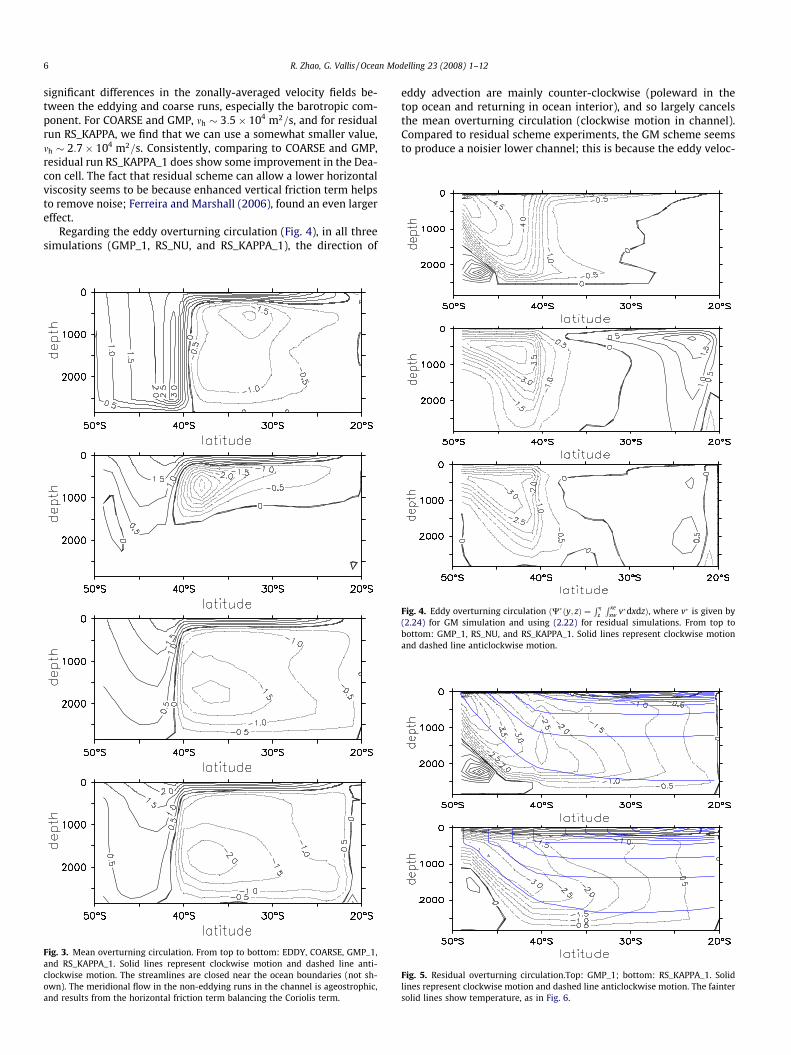
For the residual run, since the momentum equation is nowbased on the residual velocity, the eddy velocity is calculated using(2.18) and the Eulerian velocity is calculated as the difference ofthe residual velocity and the eddy velocity. The mean overturningcirculation streamfunction is defined as:

Wðy; zÞ ¼Z g

z

Z xe

xw

�vdxdz; ð4:1Þ

where �v is the Eulerian mean meridional velocity. The Eulerianmean overturning circulation in shown in Fig. 3 (from top to bot-tom: EDDY, COARSE, GMP_1 and RS_KAPPA_1). A noticeable differ-ence in mean overturning circulation for EDDY and COARSE is in theDeacon cell: the EDDY simulation has a very deep Eulerian meridi-onal circulation in channel region. This is to be expected, becausethe channel region in our model is unblocked from top to bottom,thus there is no zonal pressure gradient or topography to maintaina lateral poleward velocity in the mid of ocean interior (see (2.8));hence the downwelling in the low latitude end of the channel goesall the way down to the channel bottom. For COARSE, there is con-siderable lateral velocity in channel region, which arises because ofa balance between the Coriolis force on the meridional flow and thehorizontal viscosity, mhr2u. The latter term is needed to suppressnoise and keep the model integrations stable; of course it is chosento be as small as possible, but it is evident that it plays a non-neg-ligible role in coarse resolution simulations, and there are

scheme parameters GM scheme parameters

mmax jml Ds Agm Smax

– – – – –– – – 0.8 0.01– – – 1200 0.01– – – 1200 0.002

2 10 1200 100 – –2 2 1200 100 – –2 10 6000 100 – –2 10 12000 100 – –2 10 1200 0 – –0 – 1200 100 – –

her experiments use 2 � 1 . jh ¼ 0 for all experiments. The EDDY experiment usesization). Experiments RS_KAPPA have a constant value of j, with mrs

e ¼ jf 2=N2, andm the same initial condition which is resulted from a spin-up run (10,000-year run.


significant differences in the zonally-averaged velocity fields be-tween the eddying and coarse runs, especially the barotropic com-ponent. For COARSE and GMP, mh 3:5� 104 m2=s, and for residualrun RS_KAPPA, we find that we can use a somewhat smaller value,mh 2:7� 104 m2=s. Consistently, comparing to COARSE and GMP,residual run RS_KAPPA_1 does show some improvement in the Dea-con cell. The fact that residual scheme can allow a lower horizontalviscosity seems to be because enhanced vertical friction term helpsto remove noise; Ferreira and Marshall (2006), found an even largereffect.

Regarding the eddy overturning circulation (Fig. 4), in all threesimulations (GMP_1, RS_NU, and RS_KAPPA_1), the direction of

Fig. 3. Mean overturning circulation. From top to bottom: EDDY, COARSE, GMP_1,and RS_KAPPA_1. Solid lines represent clockwise motion and dashed line anti-clockwise motion. The streamlines are closed near the ocean boundaries (not sh-own). The meridional flow in the non-eddying runs in the channel is ageostrophic,and results from the horizontal friction term balancing the Coriolis term.

eddy advection are mainly counter-clockwise (poleward in thetop ocean and returning in ocean interior), and so largely cancelsthe mean overturning circulation (clockwise motion in channel).Compared to residual scheme experiments, the GM scheme seemsto produce a noisier lower channel; this is because the eddy veloc-

Fig. 4. Eddy overturning circulation ðW�ðy; zÞ ¼R g

z

R xexw v�dxdzÞ, where v� is given by

(2.24) for GM simulation and using (2.22) for residual simulations. From top tobottom: GMP_1, RS_NU, and RS_KAPPA_1. Solid lines represent clockwise motionand dashed line anticlockwise motion.

Fig. 5. Residual overturning circulation.Top: GMP_1; bottom: RS_KAPPA_1. Solidlines represent clockwise motion and dashed line anticlockwise motion. The faintersolid lines show temperature, as in Fig. 6.


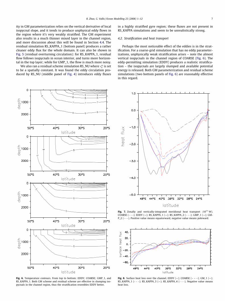
ity in GM parameterization relies on the vertical derivative of localisopycnal slope, and it tends to produce unphysical eddy flows inthe region where it’s very weakly stratified. The GM experimentalso results in a much thinner mixed layer in the channel region,and more discussion about this will be found in Section 4.4. Theresidual simulation RS_KAPPA_1 (bottom panel) produces a rathercleaner eddy flux for the whole domain. It can also be shown inFig. 5 (residual overturning circulation): for RS_KAPPA_1, residualflow follows isopycnals in ocean interior, and turns more horizon-tal in the top layer; while for GMP_1, the flow is much more noisy.

We also ran a residual scheme simulation RS_NU where mrse is set

to be a spatially constant. It was found the eddy circulation pro-duced by RS_NU (middle panel of Fig. 4) introduces eddy fluxes

Fig. 6. Temperature contours. From top to bottom: EDDY; COARSE; GMP_1, andRS_KAPPA_1. Both GM scheme and residual scheme are effective in slumping iso-pycnals in the channel region, thus the stratification resembles EDDY better.

in a highly stratified gyre region; these fluxes are not present inRS_KAPPA simulations and seem to be unrealistically strong.

4.2. Stratification and heat transport

Perhaps the most noticeable effect of the eddies is in the strat-ification. For a coarse-grid simulation that has no eddy parameter-izations, unphysically weak stratification arises – note the almostvertical isopycnals in the channel region of COARSE (Fig. 6). Theeddy-permitting simulation (EDDY) produces a realistic stratifica-tion – the isopycnals are largely slumped and available potentialenergy is released. Both GM parameterization and residual schemesimulations (two bottom panels of Fig. 6) are reasonably effectivein this regard.

Fig. 7. Zonally and vertically-integrated meridional heat transport ð1013 W).COARSE (- - -); EDDY (—); RS_KAPPA_1 (—); RS_KAPPA_2 (- - -); GMP_1 (—); GM-P_2 (- - -). Positive value means equatorward, negative value means poleward.

Fig. 8. Surface heat loss over the channel. EDDY (—); COARSE (– – –); GM_1 (—);RS_KAPPA_1 (- - -); RS_KAPPA_3 (—); RS_KAPPA_4 (- - -). Negative value meansheat loss.

Fig. 9. Zonal velocity is averaged over entire channel both zonally and meridionally.COARSE (- - -); EDDY (—); RS_KAPPA_1 (—); RS_KAPPA_2 (- - -); GMP_1 (—); GMP_2(- - -).


The total meridional heat transport, qCpR

z

Rx vTdxdz, is plotted

in Fig. 7, where negative value indicates that heat transport inthe ocean is mainly poleward. The channel region is very activein the eddying simulation, full of mesoscale eddies that transportheat polewards. With no effective eddy parameterization scheme,COARSE has a cooler channel region than EDDY (Fig. 6) and weakerheat exchange between air and sea in the pole end (determined bythe difference between SST and restoring temperature). Both GMand residual scheme simulation results show improvements forheat transport in channel region (data lines sit between EDDY

Fig. 10. Meridional velocity is averaged over entire channel both zonally and me-ridional, Ekman layer excluded. COARSE (- - -); EDDY (—); RS_KAPPA_1 (—); RS_-KAPPA_2 (- - -); GMP_1 (—); GMP_2 (- - -).

and COARSE). The improvements in both schemes are done mainlyby adding a poleward eddy velocity in the near surface region ofthe channel. Here we show two GM simulations, both withj ¼ 1200 m2 s�1, but with Smax of 0.002 to 0.01 respectively andtwo residual scheme simulations with mmax ¼ 10 or 2m2 s�1,respectively. (See Section 4.4 for the rationale of the choice ofSmax. The larger value of Smax results in a larger poleward heattransport, because of a strong eddy circulation.) It indicates thatthe poleward heat transport is somewhat improved by increasingthe value of mmax or Smax. Among the four parameterized simula-tions, the residual scheme with mmax ¼ 10 gives the closest simula-tion to EDDY.

As we noted previously, the diabatic process of lateral heat dif-fusion is not negligible in the top ocean surface diabatic layer, andin the GM scheme the tapering of the isopycnal mixing produces ahorizontal, and so diabatic, mixing of buoyancy near the surface.We incorporate this effect in the residual scheme via the termrh � ðjmlrhTÞ in (3.8). This term plays a role in transporting heatdown-gradient and has a direct influence on the surface heat ex-change between the air and sea. We increase jml (only applied tothe top 100 m) from 1200 m2=s (in RS_KAPPA_1 and RS_KAPPA_2)to 6000 m2=s (RS_KAPPA_3) and then to 12;000 m2=s (RS_KAP-PA_4; Fig. 8). It is clear that higher eddy diffusivity helps to trans-port heat poleward, and the air-sea heat exchange at the pole endof the channel is largely enhanced: the surface heat loss at 49 �S isalmost doubled as jml is increased from 1200 m2=s to 12;000 m2=s,with the latter solution better resembling the eddy-permitting re-sults, although the comparison is still not perfect.

4.3. Zonal and meridional transport

Figs. 9 and 10 plot the zonal velocity and meridional velocityprofiles against ocean depth. For zonal transports, the eddyingrun differs primarily in that it has a higher total zonal transport

Fig. 11. Horizontal structure of zonal velocity (zonally and vertically averaged).EDDY (—); COARSE (- - -); RS_KAPPA_1 (—); GM_1 (—).

Fig. 12. Sea surface height. EDDY (—); COARSE (- - -); RS_KAPPA_1 (—); GM_1 (—).


(vertically-integrated mass flux), primarily a barotropic transport.This partly a matter of friction: wall friction is only applied tothe end grid box next to the wall, and for eddy-permitting run, thislayer is much thinner comparing to coarse-grid simulations. Also,the eddying run results in a warmer and less stratified channel,hence Py does not change much over depth therefore the verticalshear of u in eddying run is small too. The low transport is a featureof both the GM and residual runs, and is not a consequence of thelarger vertical viscosity in the residual model. None of the eddyparameterization scheme shows improvement on zonal totaltransport over the scheme with high horizontal diffusion.

It seems that the eddy parameterization schemes (both the GMand residual scheme) improves vertical structure of zonal andmeridional velocity (Fig. 9). A disadvantage for residual schemeis noted that both zonal and meridional velocity are now derivedquantities from residual velocity and eddy velocity. But overall,we found both zonal and meridional velocity from residual schemeare close to the ones from GM scheme.

Although it is shown in Section 4.2 that eddy parameterizationschemes help to improve the heat transport in the ocean, it isfound that they do not have much influence on the vertically-inte-

Fig. 13. Zonally integrated eddy velocity in channel center box (sv) for top 600 m.GM parameterization (- - -); residual scheme two-step tapering (—); and residualscheme one-step tapering (—). The GM parameterization tends to produce step-likechanges in eddy velocity in the upper ocean, whereas the residual scheme issomewhat smoother.

Fig. 14. Variation of Smax and mmax on stratification. Top: GMP_1 (black) and GMP_2(red); Bottom: RS_KAPPA_1 (black) and RS_KAPPA_2 (red) (For interpretation of thereferences to colour in this figure legend, the reader is referred to the web version ofthis article.).

grated mass transport. The solutions of vertically-integrated zonaltransport and sea surface height are shown in Figs. 11 and 12,respectively. It is clear that the EDDY simulation results in a muchhigher zonal transport in the channel region, and also a much high-er sea surface height gradient, but neither the residual schemeparameterization nor GM parameterization offers much improve-ment over the COARSE experiment. In some sense, their effectsare actually working in an opposite way, that is, both GM andresidual run result in a slightly lower zonal transport and SSH gra-dient than COARSE. (The positive side of the story is that the resid-ual scheme and GM scheme give very similar results for thebarotropic mode, despite significant differences in eddy parame-terization implementations.) Certainly, the coarse models do not

Fig. 15. Eddy overturning circulation for top 1000 m, obtained with two differentvalues of Smax in the GM scheme (top two panels) and two different values of mmax inthe residual scheme (bottom two panels). From top to bottom: GMP_1; GMP_2;RS_KAPPA_1; and RS_KAPPA_2.


account for any flux of momentum into the jet region by the ed-dies, and this may account for part of the difference.

4.4. Variation of tapering parameters

As discussed in Section 2.3, one advantage of the tapering treat-ment of residual scheme is that it provides a gradual transitionfrom ocean interior to the top diabatic layer. In contrast, slopetapering of the current GM parameterization in GFDL ocean modelsometimes results in sharp shears in eddy velocity. Fig. 13 shows acomparison of the eddy velocity from both GM and residual simu-lations. The plotted lines in the figure are the eddy velocities aty = 45 �S (the center of the channel region) and zonally integrated.It is clear that for GM (dashed line), slope tapering results in asharp shear in eddy velocity before it is tapered to be a constantfor the top 300 m. For the residual scheme, the transition in v� fromocean interior to top diabatic boundary layer happens in a muchthicker layer (solid red line in Fig. 13), thus a very sharp shear ineddy velocity is avoided. It is noted that a smoother transitionfor v� from ocean interior up not only improves numerical stability,but also it seems to avoid overly slumping local isopycnals, andthus is favored for both numerical and physical reasons. We mightexpect the residual scheme to give a relatively smooth transitionfrom the ocean top to the interior, because the presence of a highviscosity and a relatively high Ekman number me=ðfH2Þ (comparedto the integrations using GM) and large Ekman depth DEk ¼ðme=f Þ1=2 will militate against jumps in the velocity field. A valueof me ¼ 10 m2 s�1 (the maximum allowed value) gives DEk �300 m, although such a deep Ekman-like layer is not necessarilya realistic aspect of the residual scheme.

A set of simulations were performed to study the model sensi-tivity as we vary the tapering parameters. We ran two simulationswith different tapering setting for both the residual scheme andGM. For GM, Smax is varying from 0.002 to 0.01. A corresponding

Fig. 16. Stratification(left) and eddy streamfunction(right). Upper panels (RS_KAPPA_5)residual scheme; bottom panel (RS_KAPPA_1): eddy velocity is forced to be constant fo

variation in mmax is approximately from 2 to 10 because, from(2.15),

me

S¼ jf 2

�ðg=q0Þqy¼ jf 2

ðg=q0ÞaTy� 103; ð4:2Þ

so that mmax � 103 Smax.The top panel of Fig. 14 is used to show the model sensitivity on

stratification to Smax in GM simulation. In the GM simulation thestratification for top channel becomes very different as Smax ischanged from 0.002 to 0.01. In contrast, the stratification of resid-ual scheme simulations is only slightly altered (bottom panel ofFig. 14) as mmax is changed from 2 to 10.

Fig. 15 shows a direct comparison between the eddy circulationstreamfunction (top 1000 m) from both GM and RS_KAPPA. Thetop two panels are GM simulations with Smax of 0.01 and 0.002,respectively. Evidently, the GM integrations give rather differentdiabatic surface layer as a different Smax is chosen: Smax ¼ 0:01 re-sults in a very thin diabatic surface layer with high eddy velocity,whereas Smax ¼ 0:002 results in a thicker diabatic layer with loweddy velocity. The two bottom panels are residual simulations withmmax of 10 and 2, respectively. It is clear that the eddy flux in theresidual simulation is much more stable to the variation of mmax.

We also tested a much more simple tapering treatment forresidual scheme, that is, only me is capped using (2.20) and withno additional treatment to force eddy velocity to be constant forocean top layer. A typical eddy velocity profile is shown inFig. 13 (solid black line): there is a shear for eddy velocity through-out the surface boundary layer except the topmost boundary,where the eddy velocity has zero shear and wind forcing is purelyapplied to Eulerian mean velocity. This treatment is equivalent tothe 2-step tapering of residual scheme but with Ds ¼ 0. Comparedthis simple treatment to the residual 2-step treatment, we find thatthis simplification does not, in fact, make much difference on themodel results except close to the surface. Fig. 16 shows both the

: eddy velocity is not enforced to be constant for the top surface diabatic layer inr the top 100 m.


stratification and eddy streamfunction (top 1000 m); both stratifi-cation and eddy circulation structure are in reasonably good agree-ment. This result is encouraging because it shows that theparameterization is not especially sensitive to rather ill-under-stood treatments of the mixed layer. The simple treatment alsoobviates the need to set Ds, which involves either an involvednumerical calculation or an arbitrary guess, neither of which iswholly satisfying.

This improvement of residual scheme occurs mainly because itstapering treatment eliminates the abrupt change in eddy velocitythat arises in the GM slope tapering treatment. It is possible thatimprovements may be realized by the use of a transitional layerbeneath the mixed layer, but the exploration of that scheme is be-yond the scope of this paper.

4.5. Diffusing potential vorticity

Potential vorticity, being a materially conserved quantity, is inmany ways a natural candidate for diffusion. (The first paper to dis-cuss potential vorticity mixing in an ocean context was probablyWelander (1973), followed by, and more explicitly looking atparameterizations, Marshall (1981), Treguier et al. (1997) andGreatbatch (1998). See Vallis (2006) for a general discussion ofthe matter.) However, in the implementations described above(both for the GM and residual schemes) we have not in fact in-cluded the gradient of potential vorticity due to planetary rotation;our schemes might be regarded as potential vorticity diffusion onthe f-plane. In this section we redress that balance, and includethe planetary vorticity gradient; however, at least in the simula-

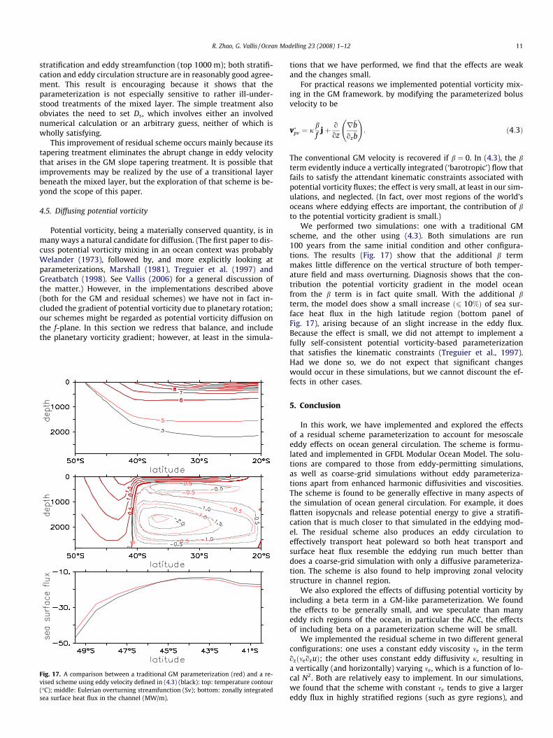
Fig. 17. A comparison between a traditional GM parameterization (red) and a re-vised scheme using eddy velocity defined in (4.3) (black): top: temperature contour(�C); middle: Eulerian overturning streamfunction (Sv); bottom: zonally integratedsea surface heat flux in the channel (MW/m).

tions that we have performed, we find that the effects are weakand the changes small.

For practical reasons we implemented potential vorticity mix-ing in the GM framework. by modifying the parameterized bolusvelocity to be

v�pv ¼ jbf

jþ o

ozr�b

oz�b

!: ð4:3Þ

The conventional GM velocity is recovered if b ¼ 0. In (4.3), the bterm evidently induce a vertically integrated (‘barotropic’) flow thatfails to satisfy the attendant kinematic constraints associated withpotential vorticity fluxes; the effect is very small, at least in our sim-ulations, and neglected. (In fact, over most regions of the world’soceans where eddying effects are important, the contribution of bto the potential vorticity gradient is small.)

We performed two simulations: one with a traditional GMscheme, and the other using (4.3). Both simulations are run100 years from the same initial condition and other configura-tions. The results (Fig. 17) show that the additional b termmakes little difference on the vertical structure of both temper-ature field and mass overturning. Diagnosis shows that the con-tribution the potential vorticity gradient in the model oceanfrom the b term is in fact quite small. With the additional bterm, the model does show a small increase ð6 10%Þ of sea sur-face heat flux in the high latitude region (bottom panel ofFig. 17), arising because of an slight increase in the eddy flux.Because the effect is small, we did not attempt to implement afully self-consistent potential vorticity-based parameterizationthat satisfies the kinematic constraints (Treguier et al., 1997).Had we done so, we do not expect that significant changeswould occur in these simulations, but we cannot discount the ef-fects in other cases.

5. Conclusion

In this work, we have implemented and explored the effectsof a residual scheme parameterization to account for mesoscaleeddy effects on ocean general circulation. The scheme is formu-lated and implemented in GFDL Modular Ocean Model. The solu-tions are compared to those from eddy-permitting simulations,as well as coarse-grid simulations without eddy parameteriza-tions apart from enhanced harmonic diffusivities and viscosities.The scheme is found to be generally effective in many aspects ofthe simulation of ocean general circulation. For example, it doesflatten isopycnals and release potential energy to give a stratifi-cation that is much closer to that simulated in the eddying mod-el. The residual scheme also produces an eddy circulation toeffectively transport heat poleward so both heat transport andsurface heat flux resemble the eddying run much better thandoes a coarse-grid simulation with only a diffusive parameteriza-tion. The scheme is also found to help improving zonal velocitystructure in channel region.

We also explored the effects of diffusing potential vorticity byincluding a beta term in a GM-like parameterization. We foundthe effects to be generally small, and we speculate than manyeddy rich regions of the ocean, in particular the ACC, the effectsof including beta on a parameterization scheme will be small.

We implemented the residual scheme in two different generalconfigurations: one uses a constant eddy viscosity me in the termozðmeozuÞ; the other uses constant eddy diffusivity j, resulting ina vertically (and horizontally) varying me, which is a function of lo-cal N2. Both are relatively easy to implement. In our simulations,we found that the scheme with constant me tends to give a largereddy flux in highly stratified regions (such as gyre regions), and


results in a somewhat overly active eddy circulation there; thisscheme generally compares less well with the eddy-permittingsimulation. To improve the simulation in the gyre region, a hori-zontal structure could perhaps be applied to me, reducing its valueat low latitudes (as in Ferreira and Marshall, 2006). However, thesimpler residual scheme with constant j (and so a variable me inthe momentum equation, that is small in regions of high stratifica-tion) shows noted improvements over all other coarse-grid runstested, and no geographical tuning of coefficients is needed. Theaddition of an enhanced horizontal buoyancy mixing in the upperocean also provides improvement in the horizontal heat transport,emphasizing the important role of the surface diabatic layer.

The solutions are also compared to those from simulationsthat use a more traditional Gent-McWilliams (GM) parameteriza-tion. The residual scheme shows certain advantages in detailcompared to GM. Primarily, the residual scheme seems less sen-sitive to the details of the implementation near the surface andto the details of the parameters. In this paper we explored var-ious options, one in which we forced the eddy velocity to beconstant over a mixed layer and another without such a con-straint. In both cases we cap me to a maximum value wherestratification is weak, in order to avoid numerical instability.Both cases achieve a gradual transition from ocean interior tothe surface diabatic layer, and their model solutions agree witheach other well except near the surface. In some contrast, wefound GM to be rather sensitive to the tapering parameterSmax, sometimes producing sudden shears in eddy velocity. Sec-ondarily, the residual scheme increases the numerical stabilityof coarse-grid runs by increasing vertical friction, enabling arather lower horizontal friction to be used. The reduction issmall in our simulations, but nonetheless welcome. Nonetheless,we certainly do not claim that the scheme is superior to the GMscheme.

The residual scheme has a somewhat simpler form than GM,and can be easily implemented by manipulating the vertical fric-tion, with the caveat that, depending on the form of the imple-mentation, isopycnal slopes must still be calculated. If there ismore than one tracer in the model, the residual scheme onlyneeds to be implemented in one equation (i.e., the momentumequation) rather than all the tracer equations, except that theRedi diffusion must still be calculated. The main disadvantageof the residual scheme for some purposes is that it uses residualvelocity as the prognostic velocity, and so an additional compu-tation may be needed to deduce Eulerian velocity.

Our overall conclusion is that the residual scheme is a viablealternative to the GM scheme. Compared to GM, the scheme iseasier to implement in a model that has no salinity or passivetracers, and is comparably easy to implement in more realisticsettings. The direct prediction of a residual velocity may beconsidered either an advantage or a disadvantage, dependingon the setting and the desired use of the model. Neither GMnor the residual scheme are perfect, and both require tuning.Our feeling is that, ideally, an ocean model should provide bothGM and a residual parameterization schemes, and the user maychoose.

Acknowledgement

We thank Richard Greatbatch and an anonymous reviewer fortheir useful comments. The work was funded by NSF and NOAAunder a CPT on eddies and the mixed layer.

Appendix A. Eddy streamfunction and eddy velocity

Expanding (2.4a,b), we have

W ¼ �1

j r�bj2

i j k

u0b0 v0b0 w0b0

�bx�by

�bz

�� ðA:1Þ

and taking �bx � �bz and �by � �bz, W can be simplified to give

W � �� iv0b0

�bzþ j

u0b0

�bzðA:2Þ

with a corresponding eddy velocity

v� ¼i j kox oy oz

�ðv0b0=�bzÞ ðu0b0=�bzÞ 0

�� ¼

�ozðu0b0=�bzÞ�ozðv0b0=�bzÞ

oxðu0b0=�bzÞ þ oyðv0b0=�bzÞ

2664

3775:ðA:3Þ

References

Andrews, D.G., Holton, J.R., Leovy, C.B., 1987. Middle Atmosphere Dynamics.Academic Press.

Eden, C., Greatbatch, R.J., Olbers, D., 2007. Interpreting eddy fluxes. J. Phys. Oceanog.37, 1282–1296.

Ferreira, D., Marshall, J., 2006. Formulation and implementation of a ‘‘residual-mean” ocean circulation model. Ocean Modell. 13, 86–107.

Gent, P.R., McWilliams, J.C., 1990. Isopycnic mixing in ocean circulation models.J. Phys. Oceanogr. 20, 150–155.

Gent, P.R., Willebrand, J., McDougall, T.J., McWilliams, J.C., 1995. Parameterizingeddy induced transports in ocean circulation models. J. Phys. Oceanogr. 25,463–474.

Gnanadesikan, A., Griffies, S.M., Samuels, B.L., 2007. Effects in a climate model ofslope tapering in neutral physics schemes. Ocean Modell. 16, 1–16.

Gough, W.A., Welch, W.J., 1994. Parameter space exploration of an ocean generalcirculation model using an isopycnal mixing parameterization. J. Mar. Res.,773–796.

Greatbatch, R.J., 1998. Exploring the relationship between eddy-induced transportvelocity, vertical momentum transfer and the isopycanl flux of potentialvorticity. J. Phys. Oceanogr. 28, 422–432.

Greatbatch, R.J., Lamb, K.G., 1990. On parameterizing vertical mixing of momentumin non-eddy-resolving ocean models. J. Phys. Oceanogr. 20, 1634–1637.

Greatbatch, R.J., Li, G., 1990. Alongslope mean flow and an associated upslope bolusflux of tracer in a parameterization of mesoscale turbulence. Deep Sea Res. 47,709–735.

Griffies, S.M., 1998. The Gent-McWilliams skew-flux. J. Phys. Oceanogr. 28, 831–841.

Griffies, S.M., Gnanadesikan, A., Pacanowski, R.C., Larichev, V.D., Dukowicz, J.K.,Smith, R.D., 1998. Isoneutral diffusion in a z-coordinate model. J. Phys.Oceanogr. 28, 805–830.

Holloway, G., 1997. Eddy transport of thickness and momentum in layer and levelmodels. J. Phys. Oceanogr. 27, 1153–1157.

Kuo, A., Plumb, R.A., Marshall, J., 2005. Transformed Eulerian mean theory. II:potential vorticity homogenization, and the equilibrium of a wind- andbuoyancy-driven zonal flow. J. Phys. Oceanogr, 175–187.

Ledwell, J.R., Watson, A.J., Law, C.S., 1998. Mixing of a tracer in the pycnocline.J. Geophys. Res. 103 (C10), 21499–21530.

Marshall, J.C., 1981. On the parameterization of geostrophic eddies in the ocean.J. Phys. Oceanogr. 11, 257–271.

Redi, M.H., 1982. Isopycnal mixing by coordinate rotation. J. Phys. Oceanogr. 12,1154–1158.

Toole, J.M., Schmitt, R.W., Polzin, K.L., 1994. Estimates of diapycnal mixing in theabyssal ocean. Science, 1120–1123.

Treguier, A.M., Held, I.M., Larichev, V.D., 1997. On the parameterization of thequasigeostrophic eddies in primitive equation ocean models. J. Phys. Oceanogr.27, 567–580.

Vallis, G.K., 2006. Atmospheric and Oceanic Fluid Dynamics. Cambridge UniversityPress. p. 745.

Wardle, R., Marshall, J., 2000. Representation of eddies in a primitive equationmodel by a PV flux. J. Phys. Oceanogr. 30, 2481–2503.

Welander, P., 1973. Lateral friction in the ocean as an effect of potential vorticitymixing. Geophys. Fluid Dynam. 5, 101–120.

ocean modelling - geophysical fluid dynamics … mesoscale eddies with residual and eulerian...

Documents