oceanographic characteristics of biological hot spots in ......oceanographic characteristics of...

ARTICLE IN PRESS

0967-0645/$ - se

doi:10.1016/j.ds

�Correspondital Research Di

CA 93940-2097

E-mail addre

Deep-Sea Research II 53 (2006) 250–269

www.elsevier.com/locate/dsr2

Oceanographic characteristics of biological hot spots in theNorth Pacific: A remote sensing perspective

Daniel M. Palaciosa,b,�, Steven J. Bogradb, David G. Foleya,b, Franklin B. Schwingb

aJoint Institute for Marine and Atmospheric Research, University of Hawaii, 1000 Pope Road, Marine Sciences Building,

Room 312, Honolulu, HI 96822, USAbNOAA/NMFS/SWFSC/Environmental Research Division, 1352 Lighthouse Avenue, Pacific Grove, CA 93950-2097, USA

Received 20 May 2005; accepted 5 February 2006

Available online 27 April 2006

Abstract

Biological hot spots in the ocean are likely created by physical processes and have distinct oceanographic signatures.

Marine predators, including large pelagic fish, marine mammals, seabirds, and fishing vessels, recognize that prey

organisms congregate at ocean fronts, eddies, and other physical features. Here we use remote sensing observations from

multiple satellite platforms to characterize physical oceanographic processes in four regions of the North Pacific Ocean

that are recognized as biological hot spots. We use data from the central North Pacific, the northeastern tropical Pacific,

the California Current System, and the Galapagos Islands to identify and quantify dynamic features in terms of spatial

scale, degree of persistence or recurrence, forcing mechanism, and biological impact. The dominant timescales of these

processes vary from interannual (Rossby wave interactions in the central North Pacific) to annual (spring-summer

intensification of alongshore winds in the California Current System; winter wind outflow events through mountain gaps

into the northeastern tropical Pacific), to intraseasonal (high-frequency equatorial waves at the Galapagos). Satellite

oceanographic monitoring, combined with data from large-scale electronic tagging experiments, can be used to conduct a

census of biological hot spots, to understand behavioral changes and species interactions within hot spots, and to

differentiate the preferred pelagic habitats of different species. The identification and monitoring of biological hot spots

could constitute an effective approach to marine conservation and resource management.

r 2006 Elsevier Ltd. All rights reserved.

Keywords: Biological hot spots; Remote sensing; Upwelling; Eddies; Equatorial waves; Pacific Ocean

1. Introduction

Oceans are naturally heterogeneous on a widerange of spatial scales. The complexity of thisenvironment creates a variety of habitats that

e front matter r 2006 Elsevier Ltd. All rights reserved

r2.2006.03.004

ng author. NOAA/NMFS/SWFSC/Environmen-

vision, 1352 Lighthouse Avenue, Pacific Grove,

,USA. Fax: +1831 648 8440.

ss: [email protected] (D.M. Palacios).

marine organisms exploit throughout their lifehistories. Species have evolved to recognize andutilize particular features of their environment forlocating food, avoiding predation, finding a mate,and producing young. Marine populations also tendto aggregate for reproduction, feeding, protection,and migration. Their ability to perform thesefunctions is dependent not only on cues from otherorganisms, but on features of their physicalenvironment. Locations where organisms tend to

.

www.elsevier.com/locate/dsr2

dx.doi.org/10.1016/j.dsr2.2006.03.004

mailto:[email protected]

ARTICLE IN PRESSD.M. Palacios et al. / Deep-Sea Research II 53 (2006) 250–269 251

concentrate regularly, or where there is highbiological activity, are termed ‘‘biological hotspots’’. Because these areas feature high concentra-tions of organisms, including many species that arecommercially exploited, they are often targeted forresource harvesting. Thus, biological hot spots mustbe an important facet of resource management andconservation efforts, including determining how toimplement marine protected areas (MPAs), refugia,and fishery closures (Worm et al., 2003; Block et al.,2005).

A critical requirement in ecosystem-based re-source management is learning how to define andidentify biological hot spots, and characterizingthem within the overall ocean environment. Oneaspect of this is to determine which physicalattributes define a hot spot from an organism’spoint of view. This can be done through electronictagging studies, which provide information onspecies aggregations and interactions in the contextof the environment they are sampling (Block et al.,2002, 2005). A parallel effort is to assess thecharacteristics (e.g., size, life span, seasonality,persistence) of observable ocean features that couldaffect biological productivity and animal distribu-tions. The combined use of these approaches allowsfor a more complete description of biological hotspots and a better understanding of pelagic habitatutilization by a variety of species.

Until recently, our understanding of the relation-ship between physical ocean structure and thedistribution and behavior of top predators waslimited to anecdotal reports, opportunistic sam-pling, simple correlations, and studies of limitedtemporal or spatial scope. Remote sensing has nowbecome a powerful tool for monitoring oceanconditions on a global scale and at high spatialand temporal resolution. In addition, satellite dataare increasingly being used to derive relevantecosystem indicators (e.g., Polovina and Howell,2005). In this paper, we use remote sensingobservations from multiple satellite platforms todescribe the oceanographic characteristics of fourdistinct environments in the North Pacific thatencompass recognized biological hot spots, in termsof spatial scale, degree of persistence, recurrence,forcing mechanism, and biological impact. We alsopresent a number of analytical approaches tocharacterize dynamic physical features that maylead to formation of biological hot spots in thesedifferent environments. This study provides aframework for a more complete characterization

of biological hot spots that includes the oceano-graphic perspective.

2. Data sources and methods

2.1. Bathymetry

Digital bathymetry was extracted from the globalsea floor topography of Smith and Sandwell (1997),version 8.2 (November 2000). This data set com-bines all available depth soundings with high-resolution marine gravity information provided bythe Geosat, ERS-1/2, and TOPEX/Poseidon (T/P)satellite altimeters. It is available on line from theInstitute of Geophysics and Planetary Physics at theScripps Institution of Oceanography (http://topex.ucsd.edu/). The data set has a nominal resolution of2 arc minutes (�4 km). A recent assessment of thisdata set relative to high-resolution (30 and 100m)echosounder-derived multibeam surveys in thenortheast Pacific found that the product performswell at identifying features to the scale of sea-mounts, but that subgrid-scale features in thesatellite-derived bathymetry may vary from theirtrue depth by up to 50% (Etnoyer, 2005).

2.2. Sea-level anomalies

Global, 7-day maps of gridded sea-level anoma-lies (SLA; i.e., the difference between the observedsea-surface height and the mean sea level, in cm) at1/3-degree resolution on a Mercator projection (i.e.,�37 km at the equator and �18.5 km at 601N/S)were obtained for the period 14 October 1992–18August 2004. SLA are relative to a 7-year mean(January 1993–January 1999). These maps areproduced by combining data from the T/P, ERS-1/2, Jason, and Envisat satellite altimeters using themethod described in Ducet et al. (2000). The dataare produced by the Centre National d’etudesSpatiales (CNES, France) in partnership with itssubsidiary Collecte, Localisation, Satellites (CLS)and local industry, for the Segment Sol multi-missions d’ALTimetrie, d’Orbitographie et de loca-lisation precise multimission ground segment(Ssalto) program, as part of the Data Unificationand Altimeter Combination System (Duacs). Thedata are distributed by the Archiving, Validation,and Interpretation of Satellite Oceanographic data(Aviso) project (http://www.aviso.oceanobs.com/).Despite sampling error issues due to differingground tracks and orbit repeat periods among

http://topex.ucsd.edu/

http://topex.ucsd.edu/

http://www.aviso.oceanobs.com/

ARTICLE IN PRESSD.M. Palacios et al. / Deep-Sea Research II 53 (2006) 250–269252

several altimeter instruments, merged data frommultiple missions have the advantage of resolvingoceanic mesoscale processes, which is beyond thecapabilities of a single instrument (Fu et al., 2003).

2.3. Ocean color

Satellite-derived ocean color (phytoplanktonchlorophyll-a concentration, or CHL, in mgm�3)measured by the Sea-viewing Wide-Field-of-viewSensor (SeaWiFS) was obtained from a variety ofsources for different purposes. For the generalcharacterization in Section 3, we used monthlyaverages for the period September 1997–December2004 at 9-km resolution. Selected monthly and8-day averages were used for the case studies of thecentral North Pacific and the northeastern tropicalPacific in Sections 4.1 and 4.3, respectively. These9-km data sets were obtained from the NASAGoddard Space Flight Center’s (GSFC) EarthSciences Data and Information Services CenterDistributed Active Archive Center (GES DISCDAAC) (http://disc.gsfc.nasa.gov).

For the case study of the central CaliforniaCurrent System in Section 4.2, daily SeaWiFSlevel-1a, Local-Area-Coverage (LAC) raw radianceswere compiled from three sources for the periodOctober 1997–March 2005. For October 1997–December 2004 data were provided by the Monter-ey Bay Aquarium Research Institute (MBARI) incollaboration with the University of California atSanta Cruz (UCSC) and NASA GSFC. For July1998, data from MBARI’s ground station were notavailable; data acquired by the University ofCalifornia at Santa Barbara (UCSB) ground stationand distributed by the GES DISC DAAC were usedin their place. For January–March 2005 data weresupplied by the NOAA National Ocean Service andNOAA CoastWatch under license to ORBIMAGE,Inc. The compiled raw radiances were processedto level-3 monthly mean CHL and projected ontoa 0.0125� 0.0125-degree resolution grid usingNASA’s SeaDAS software.

Finally, for the case study of the GalapagosIslands region in Section 4.4, daily level-2 MergedLocal Area Coverage (MLAC) CHL data wereobtained from NASA’s Ocean Biology ProcessingGroup (OBPG) distribution point (http://oceancolor.gsfc.nasa.gov/) for the period 4 October 1997–23December 2004. Daily spatial subsets for the areabounded by 95–911W, 21S–11N were processed to

8-day averages at a 0.0125-degree (1.39-km) resolu-tion in SeaDAS.

2.4. Sea-surface temperature

Sea-surface temperatures (SST) derived from theAdvanced Very High Resolution Radiometer(AVHRR) and processed with the NOAA/NASAAVHRR Oceans Pathfinder algorithm version 4.1are distributed by the Physical OceanographyDistributed Active Archive Center (PO.DAAC) atthe NASA/California Institute of Technology JetPropulsion Laboratory (JPL) (http://poet.jpl.nasa.gov/). An 8-day average of best-quality, ascending-pass (daytime) data at 9 km resolution for theperiod 2–9 February 2003 is used in Section 4.3 toillustrate the case study of the northeastern tropicalPacific.

2.5. Analysis of monthly ocean color for central

California

The combined data set of 0.0125-degree monthlyCHL covering the period October 1997–March 2005comprised 90 images. Empirical orthogonal func-tion (EOF) analysis (Emery and Thomson, 1997; seealso Kelly, 1988) of this data set was used to extractthe characteristic patterns of CHL variability andidentify potential biological hot spots off centralCalifornia. Prior to analysis, a 5� 5-pixel mediansmoother was applied to each image to removesmall-scale noise. Few pixels were missing in mostimages due to persistent cloudiness, and these wereinterpolated with a single pass of a 5� 5 medianfilter. The images for November 1997 and July 1998had substantial gaps, and additional passes with7� 7 and 11� 11 median filters were necessary tofill those gaps. After gap filling, each monthly imagecontained 151,249 valid pixels. Log-transformationof these data was necessary to homogenize thevariance, an assumption of the EOF technique. Tohighlight potential biological hot spots (i.e. areas ofenhanced CHL), the spatial mean was removedfrom each image (this approach is analogous tospatial detrending by removing the large-scalecomponent in order to emphasize local variationsabove or below the spatial mean). The final step inthe pre-treatment of the data set was the removal ofthe temporal mean at each pixel location. Theresults of the EOF analysis on these 151,249 spatialpoints (pixels) by 90 time steps (months) arepresented in Section 4.2.

http://disc.gsfc.nasa.gov

http://oceancolor.gsfc.nasa.gov/

http://oceancolor.gsfc.nasa.gov/

http://poet.jpl.nasa.gov/

http://poet.jpl.nasa.gov/


2.6. An index for the Galapagos plume

The physical and ecological factors leading to aplume of high phytoplankton biomass on thewestern side of the Galapagos Archipelago aredescribed in Section 3.1.4. In order to quantify thescales of variability in this dynamic region, we usedthe 8-day CHL averages at 0.0125-degree (1.39-km)resolution for the area bounded by 95–911W,21S–11N. This data set comprised 329 imagescovering the period 4 October 1997–23 December2004. Small-scale noise in each image was removedwith a 3� 3 median filter. The number of pixels ineach image containing CHL X0.5mgm�3 (a con-tour level that efficiently delineates the plume) wasobtained and a Galapagos Plume Index (GPI) wasderived by computing the area covered by thesepixels. The total CHL biomass contained in thisarea was also computed. The resulting GPI timeseries are presented and discussed in Section 4.4.

3. Oceanographic characteristics of biological hot

spots in the North Pacific

Biological hot spots are most often regarded asregions where top predators aggregate (Worm et al.,2003, 2005), presumably because of enhancedtrophic interactions and feeding opportunities.From dynamical considerations, physical oceano-graphic features such as eddies, meanders, and

Fig. 1. Digital bathymetry v8.2 (in km) of Smith and Sandwell (1997)

(2) central California Current System, (3) northeastern tropical Pacific,

fronts provide the mechanisms that result inaggregation and enhanced primary production(Flierl and McGillicuddy, 2002; Olson, 2002). Whilewe recognize that biological hot spots also mayoccur in ocean regions that do not have discernablephysical characteristics because they are used asfixed migratory corridors or reproductive destina-tions, our focus here is on the oceanographicfeatures that lead to biological hot spots.

Oceanographic features can vary in terms of theirspatial scales, their degree of persistence or recur-rence, their forcing mechanisms, and their biologicalimpacts. These characteristics are examined in thissection, using four representative regions thatencompass recognized biological hot spots: thecentral North Pacific (CNP), the central CaliforniaCurrent System (CCS), the northeastern tropicalPacific (NETP), and the Galapagos Islands (Fig. 1).Descriptions of the general setting and the typicalvariability of these regions are presented in thefollowing sections. Case studies illustrating theparticular dynamics and the temporal variabilityin each region are given in Section 4.

3.1. Regional setting

3.1.1. The central North Pacific

Although hot spot activity is often most intense atrelatively small spatial scales (tens of meters to a fewhundred kilometers), coherent physical features can

for four regions in the North Pacific. (1) Central North Pacific,

and (4) Galapagos Islands.


extend across entire ocean basins. The region of theNorth Pacific bounded by 27.5–451N, 1551E–1501W(Fig. 1) is representative of a number of processesthat contribute to the development of large-scale,biologically utilized physical features. The CNP isfar from coastal boundaries, is characterized bystrong latitudinal gradients in light and nutrientavailability (Glover et al., 1994; Chai et al., 2003),and is impacted by strong seasonality in large-scalewind forcing. A sharp transition from the highsurface chlorophyll concentrations of the SubarcticGyre to the low concentrations of the North PacificGyre is defined by the 0.2mgm�3 surface chlor-ophyll contour, and is known as the transition zonechlorophyll front (TZCF; Polovina et al., 2001).This frontal feature has been shown to be animportant foraging and migratory habitat for anumber of apex predators such as tuna, sea turtles,sharks, and seabirds (Laurs et al., 1984; Polovinaet al., 2000, 2001, 2004), which leads to conflictsbetween migrating protected species and commer-cial fishing. Islands, seamounts, and sharp bathy-metric gradients (Fig. 1) also contribute tothe development of mesoscale physical features(Bograd et al., 1997; Seki et al., 2001). Blue whales(Balaenoptera musculus) occur year-round onthe western part of the CNP (east of 1701E andnorth of 401N), and tend to congregate around theEmperor Seamounts in winter months (Mooreet al., 2002).

3.1.2. The central California Current System

Although a much smaller region than consideredin the previous case, the region bounded by34–401N, 1261W to the coastal boundary (Fig. 1)is characterized by very strong cross-shore gradientsin physical and biological fields, is strongly modu-lated by seasonal wind forcing and Ekman dy-namics, has a complex and energetic currentstructure, and is greatly influenced by a hetero-geneous continental shelf topography and coastalorography (Hickey, 1979). This is a highly produc-tive eastern boundary current system, driven byseasonal coastal upwelling, which maintains numer-ous economically important marine fisheries. Heavyfishing effort in this region in combination withnatural environmental variability has resulted in anumber of overfished stocks (e.g., NMFS, 1999;Jacobson et al., 2005). This region is also home to aseries of federal marine sanctuaries (Fig. 11A) andstate reserves, and is being considered for theestablishment of MPAs.

3.1.3. The northeastern tropical Pacific

Further south, the region of the eastern tropicalPacific bounded by 5–17.51N, 120–76.51W (Fig. 1)is dominated by complex offshore bathymetry andrugged coastal orography. The NETP is greatlyimpacted by wintertime wind jets passing throughmountain gaps along the Central American isthmus(Chelton et al., 2000), which lead to the develop-ment of upwelling plumes (Clarke, 1988; Legeckis,1988; Trasvina et al., 1995) and numerous west-ward-propagating eddies readily detectable in satel-lite SST and CHL imagery (Hansen and Maul,1991; Muller-Karger and Fuentes-Yaco, 2000;Gonzalez-Silvera et al., 2004). Further offshore,seasonally intensified cyclonic wind stress curlassociated with the intertropical convergencezone forces a broad thermocline ridge along 81Nbetween the westward-flowing North EquatorialCurrent and the eastward-flowing North EquatorialCountercurrent. At the eastern terminus of thisshallow ridge is the Costa Rica Dome, anothercenter of enhanced biological production in theNETP (Fiedler, 2002). The NETP is a diverse andhighly productive tropical ecosystem, which sup-ports an industrial tuna fishery and other toppredators (Reilly and Thayer, 1990; Fiedler, 2002).This region is also the stage of the tuna-dolphinconservation issue (Gerber et al., 1999; Hall andDonovan, 2001).

3.1.4. The Galapagos Islands

On smaller scales, the region bounded by21S–21N, 92.5–881W (Fig. 1) contains the Galapa-gos Islands, which represent a steep topographicbarrier within a deep oceanic environment approxi-mately 960 km off the coast of South America. Thephysical and ecological factors leading to a plume ofhigh phytoplankton biomass (CHL X0.5mgm�3)on the western side of the archipelago include thelocalized, year-round topographic upwelling of theEquatorial Undercurrent, seasonal wind-drivenupwelling along the equatorial cold tongue, andnatural iron enrichment from the island platform(Feldman, 1986; Coale, 1998; Palacios, 2002, 2004).On average, the plume covers an area of about25,000 km2 and has a westward extent of about120 km (Palacios, 2002). Its biological effects areevident from the high densities of marine mammalswithin the plume (Palacios, 1999, 2003; Palacios andSalazar, 2002; Salazar, 2002). This region is subjectto strong interannual variations (i.e. El Nino and LaNina events) that greatly impact the local marine


biota that depend on the upwelling (Boersma, 1978;Feldman et al., 1984; Robinson and del Pino, 1985;Valenti et al., 1999). This region is a textbookexample of endemism, speciation, and biodiversityresulting from strong environmental pressures(James, 1991; Grant, 1999). The oceanic regionsurrounding the Galapagos is a National MarineReserve (Fig. 5A), declared by the Government ofEcuador (Heylings et al., 2002), with a number ofserious conservation issues (e.g., Boersma et al.,2005).

3.2. The mean state

Although many hot spots are patchy andephemeral (e.g., open-ocean eddies or small-scalefronts), physical features that are relatively fixedspatially or that persist through time may be moreecologically relevant. Such persistence is conduciveto food chain development and trophic interactionsfrom primary producers up to the highly mobilenekton. Similarly, processes that repeat on regularcycles (e.g., seasonal coastal upwelling in easternboundary current systems) can lead to the pre-dictable development of exploitable foraging re-gions year after year. Many marine species haveevolved to synchronize their life cycles to thepresence (or absence) of these persistent andrepeatable features (Cushing, 1990).

Seasonal mean maps of SLA and CHL are usedto represent the background physical and biological

Fig. 2. Mean SLA (A, B; in cm) and mean CHL (C, D; in mg m�3) for

this figure and in Figs. 3–9 were smoothed with a 3� 3-pixel median fi

0.2mgm�3 contour representing the TZCF.

environments of each region, respectively, and canbe used to identify persistent and repeatable features(Figs. 2–5). Across the open CNP, SLA has largepositive and negative amplitudes along a zonal bandcentered near 30–351N, with the strongest positiveanomalies occurring in summer (Fig. 2B) over therugged submarine topography west of the dateline(Fig. 1). In winter, a persistent band of negativeanomalies extends southwest from the northwesternboundary of the Subarctic Gyre (Fig. 2A). Asso-ciated with this band of negative anomalies is thesouthward extension of the TZCF (Fig. 2C).Relatively high (low) CHL covers most of thecentral North Pacific region in winter (summer),reflecting seasonal interactions between light andnutrient availability. The TZCF migrates seasonallyover approximately 10 degrees of latitude, althoughthere is significant interannual variability in itsseasonal range and wintertime southerly extent(Bograd et al., 2004).

Compared to the CNP, the CCS has a much smallerseasonal range in SLA (Fig. 3A and B). The SLAgradients, however, can be high, and reflect importantseasonal dynamics. The cross-shore SLA gradient inthe CCS reflects the persistent equatorward flow of theCalifornia Current, while the larger offshore anomaliesin summer reflect the seasonal development andoffshore propagation of mesoscale eddies followingthe spring transition (Strub et al., 1987; Chereskinet al., 2000; Lynn et al., 2003). Long-lived mesoscaleeddies in the CCS have been implicated in retention

February and August for the central North Pacific. CHL fields in

lter to remove small-scale noise. Black line in (C) and (D) is the

ARTICLE IN PRESS

Fig. 3. Mean SLA (A, B; in cm) and mean CHL (C, D; in mgm�3) for February and August for the central California Current System.

Fig. 4. Mean SLA (A, B; in cm) and mean CHL (C, D; in mg m�3) for February and August for the northeastern tropical Pacific. Black

contour in each panel is the corresponding mean location of the Costa Rica Dome, as outlined by the 20 1C isotherm depth at 35m,

courtesy of Paul C. Fiedler (NOAA/NMFS/SWFSC). Gray line marks the axis of the East Pacific Rise.

D.M. Palacios et al. / Deep-Sea Research II 53 (2006) 250–269256

ARTICLE IN PRESS

Fig. 5. Mean SLA (A, B; in cm) and mean CHL (C, D; in mgm�3) for February and August for the Galapagos Islands. Black line in (A) is

the boundary of the Galapagos Marine Reserve, courtesy of the Unidad de Zonificacion, Servicio Parque Nacional Galapagos, Ecuador.

Yellow line in (C) and (D) is the outline of the Galapagos Plume, as indexed by the 0.5mgm�3 CHL level.

D.M. Palacios et al. / Deep-Sea Research II 53 (2006) 250–269 257

and recruitment of coastal pelagic fish species (Loger-well and Smith, 2001). Seasonal coastal upwelling inthe CCS leads to very high summertime CHL at thecoast, and strong cross-shore gradients (Fig. 3D).

There is a marked seasonal contrast in SLA in theNETP (Fig. 4A and B). In winter, a band of highanomalies extending westward from Central Amer-ica at about 10–151N reflects the persistent forma-tion of eddies in the Gulfs of Tehuantepec andPapagayo and their offshore propagation (Fig. 4A;Palacios and Bograd, 2005). A break in the highSLA along the path of Tehuantepec eddies isapparently associated with the East Pacific Rise(Palacios and Bograd, 2005). In contrast to thispattern, summer in the eastern tropical Pacific isquiescent (Fig. 4B). At this time, zonal thermoclineridging, peaking at the Costa Rica Dome, results inrelatively low mean SLA and elevated CHL (Fig. 4Band D). High wintertime CHL squirts extendoffshore from the Gulfs of Tehuantepec, Papagayo,and Panama, driven by local upwelling resulting

from intense wind jets blowing through mountaingaps along Central America (Fig. 4C). This alsoresults in negative SLAs at the Gulfs of Tehuante-pec and Papagayo (Fig. 4A). The zonal bandcharacterized by strong eddy activity in winter alsocorresponds with relatively higher CHL.

The region around the Galapagos has weakseasonality in SLA (Fig. 5A and B). SLAs aremostly negative, especially in August, when equa-torial divergence and upwelling are strongest(Palacios, 2004). The Galapagos high-CHL plumeresulting from the topographic upwelling of theEquatorial Undercurrent is present year-round, butbecomes more evident in August due to theadditional forcing of upwelling-favorable southeasttrade winds at this time of the year (Fig. 5C and D).

3.3. Variations around the mean state

Strong and persistent perturbations from themean background state in a region may be

ARTICLE IN PRESS

Fig. 6. RMS SLA (A, B; in cm) and RMS CHL (C, D; in mgm�3) for February and August for the central North Pacific.

Fig. 7. RMS SLA (A, B; in cm) and RMS CHL (C, D; in mgm�3) for February and August for the central California Current System.


ARTICLE IN PRESS

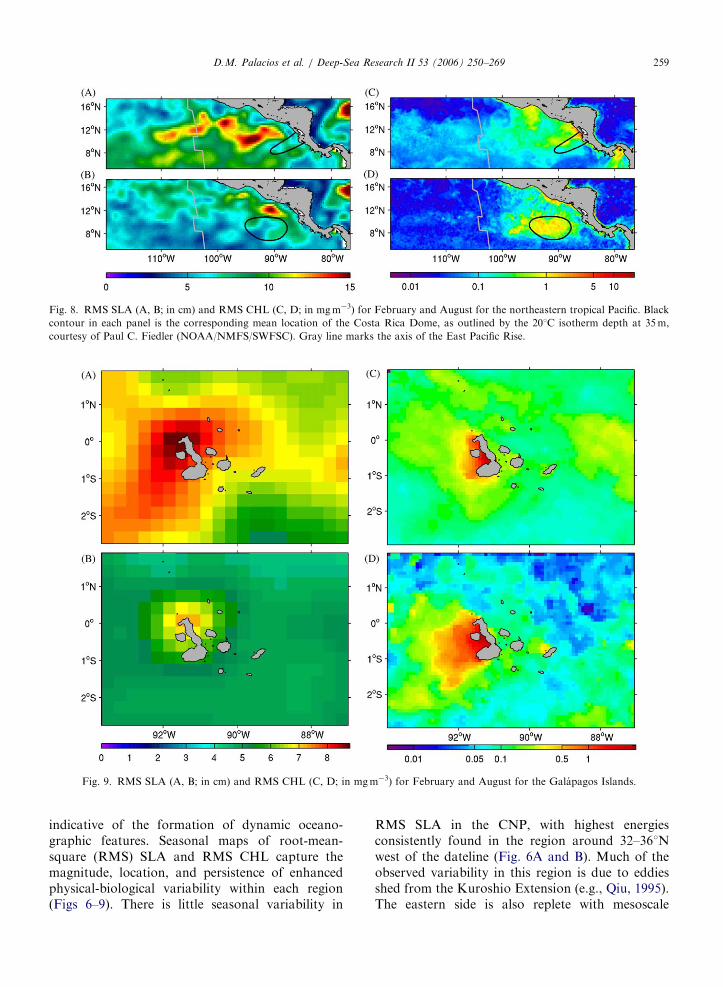
Fig. 8. RMS SLA (A, B; in cm) and RMS CHL (C, D; in mgm�3) for February and August for the northeastern tropical Pacific. Black

contour in each panel is the corresponding mean location of the Costa Rica Dome, as outlined by the 201C isotherm depth at 35m,

courtesy of Paul C. Fiedler (NOAA/NMFS/SWFSC). Gray line marks the axis of the East Pacific Rise.

Fig. 9. RMS SLA (A, B; in cm) and RMS CHL (C, D; in mgm�3) for February and August for the Galapagos Islands.


indicative of the formation of dynamic oceano-graphic features. Seasonal maps of root-mean-square (RMS) SLA and RMS CHL capture themagnitude, location, and persistence of enhancedphysical-biological variability within each region(Figs 6–9). There is little seasonal variability in

RMS SLA in the CNP, with highest energiesconsistently found in the region around 32–361Nwest of the dateline (Fig. 6A and B). Much of theobserved variability in this region is due to eddiesshed from the Kuroshio Extension (e.g., Qiu, 1995).The eastern side is also replete with mesoscale


features consistent with the passage of long Rossbywaves propagating westward from the NorthAmerican coast (e.g., van Woert and Price, 1993;Fu and Qiu, 2002). The highest variability in theRMS CHL field is coincident with the high-energyeddy field in winter, but migrates northward withthe TZCF in summer (Fig. 6C and D). The broadzones of high RMS CHL around 32–361N in winterand 38–421N in summer reflect interannual varia-bility in the seasonal range of the TZCF.

The highest eddy energies in the CCS occur in theoffshore region, and reflect the year-round presenceof the meandering California Current, as well asoffshore-propagating features associated with sum-mertime coastal upwelling (Fig. 7A and B). HighestCHL variability in the CCS is confined year-roundto the upwelling zone along the shelf, but isstrongest in the peak upwelling months in springand summer (Fig. 7C and D).

In the NETP, the winter months are characterizedby a much more energetic eddy field than thesummer months, as is evidenced by the mean SLAfields (Fig. 8A and B). Highest eddy energies arefound within the region of eddy propagation awayfrom the Central American coast. The CHLvariability responds to these seasonally varyingphysical processes (Fig. 8C and D). Winter windjets create upwelling plumes off the Gulfs ofTehuantepec, Papagayo, and Panama, as well ashighly variable CHL content in the westwardpropagating eddies. The Costa Rica Dome is moststrongly developed in summer, and correspondswith the highest CHL RMS.

SLA variability is small at the Galapagoscompared to the other regions (Fig. 9A and B). Amore energetic SLA field is seen in February,especially where the Equatorial Undercurrent up-wells. Variations within the CHL plume on thewestern side of the islands are evident throughoutthe year, but are strongest in August (Fig. 9Cand D).

4. Case studies

4.1. The central North Pacific

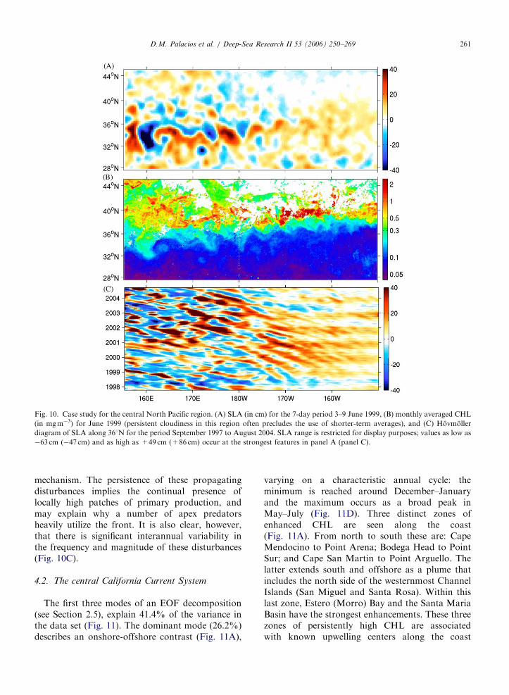
The June 1999 mean SLA and CHL fields providea case study of physical-biological coupling atoceanographic features spanning a wide rangeof spatial scales over the central North Pacific(Fig. 10). On the basin scale, the TZCF extendsfrom 371N, 1501W across the entire width of the

region to 331N, 1551E, with a well-defined wavelikepattern of �300–500 km wavelength (Fig. 10B).This is a dynamic region separating low-nutrient,oligotrophic subtropical waters to the south fromhigh-nutrient, high CHL waters to the north. TheSLA field also shows a similar wavelike patternspanning the same meridional range across thebasin, with the height anomalies intensifying to thewest (Fig. 10A).

At the mesoscale, there is a direct correspondencebetween the SLA eddy field and local CHL content.(Note that because a spatially sloping surface isremoved from the absolute altimetry measurementsof sea level, some of these features may be meandersrather than closed eddies.) The cyclonic (anti-cyclonic) features in Fig. 10 are clearly associatedwith locally high (low) CHL, reflecting the subsur-face upwelling (downwelling) associated with sur-face divergence (convergence). This coupling can beseen in the intense eddy field near the westernboundary of the region, as well as in the weaker lineof eddies that span the basin near 281N. Similarcorrespondences are found year-round in thisregion. This relationship demonstrates that thewaters within and south of the TZCF are nutrient-limited, and require vertical motions to injectnutrients into the euphotic zone and induce primaryproduction, as has been demonstrated in otheroligotrophic gyral systems (e.g., McGillicuddy andRobinson, 1997; McGillicuddy et al., 1998).

Interannual variability in SLA along 361N(Fig. 10C) reveals the persistence and westwardpropagation of the eddy field, with greatest energywest of the dateline. Alternating bands of relativelyhigh and low SLA can be tracked for two years ormore in Fig. 10C, with a westward propagationspeed of �3–5 kmd�1. This is consistent with thepropagation of first-mode baroclinic Rossby waves,which have been shown to dominate the propagat-ing component of altimetry-derived sea surfaceheight fields (Chelton and Schlax, 1996; Stammer,1997; Polito and Cornillon, 1997; Cipollini et al.,1997; Uz et al., 2001). The vertical isopycnaldisplacements associated with the negative SLAfeatures will introduce nutrients into the euphoticzone, thus stimulating primary production (Uzet al., 2001; Cipollini et al., 2001; Sakamoto et al.,2004). Uz et al. (2001) and Sakamoto et al. (2004)found a strong coherence between satellite-derivedpropagating SLA and CHL signatures in themidlatitude oceans, with nutrient injection uponpassage of Rossby waves being the dominant

ARTICLE IN PRESS

Fig. 10. Case study for the central North Pacific region. (A) SLA (in cm) for the 7-day period 3–9 June 1999, (B) monthly averaged CHL

(in mgm�3) for June 1999 (persistent cloudiness in this region often precludes the use of shorter-term averages), and (C) Hovmoller

diagram of SLA along 361N for the period September 1997 to August 2004. SLA range is restricted for display purposes; values as low as

�63 cm (�47 cm) and as high as +49 cm (+86 cm) occur at the strongest features in panel A (panel C).


mechanism. The persistence of these propagatingdisturbances implies the continual presence oflocally high patches of primary production, andmay explain why a number of apex predatorsheavily utilize the front. It is also clear, however,that there is significant interannual variability inthe frequency and magnitude of these disturbances(Fig. 10C).

4.2. The central California Current System

The first three modes of an EOF decomposition(see Section 2.5), explain 41.4% of the variance inthe data set (Fig. 11). The dominant mode (26.2%)describes an onshore-offshore contrast (Fig. 11A),

varying on a characteristic annual cycle: theminimum is reached around December–Januaryand the maximum occurs as a broad peak inMay–July (Fig. 11D). Three distinct zones ofenhanced CHL are seen along the coast(Fig. 11A). From north to south these are: CapeMendocino to Point Arena; Bodega Head to PointSur; and Cape San Martin to Point Arguello. Thelatter extends south and offshore as a plume thatincludes the north side of the westernmost ChannelIslands (San Miguel and Santa Rosa). Within thislast zone, Estero (Morro) Bay and the Santa MariaBasin have the strongest enhancements. These threezones of persistently high CHL are associatedwith known upwelling centers along the coast

ARTICLE IN PRESS

Fig. 11. Case study for the central California Current System region. The first three modes (A–C) of an EOF decomposition of monthly

averaged, 1-km resolution CHL (after log-transformation; see Section 2.5 for details) for the period October 1997–March 2005. Panels in

bottom row (D–F) show the corresponding amplitude time series (red series in the last two panels are the 5-point running averages). Black

lines in panel A are the boundaries of the NOAA-designated Cordell Bank, Gulf of the Farallones, and Monterey Bay National Marine

sanctuaries (from north to south), courtesy of Chad King (NOAA/NOS/MBNMS). Black contour in panel B is the 200-m isobath from

the Smith and Sandwell (1997) bathymetry.


(Hickey, 1979; Dorman and Winant, 1995), andpossibly represent areas of enhanced foragingopportunities for migratory species and top pre-dators in the CCS.

The second (9.1% of the variance) and third(6.1%) modes are characterized by high-frequencyvariability (Fig. 11E and F) possibly representingshort-lived events not fully resolved by the monthlycomposites. However, a clear interannual signal isalso present in both modes (as illustrated by the 5-point running averages in Fig. 11E and F). Mode 2describes a narrow band of CHL enhancementalong the coast that widens northward of SanFrancisco Bay (Fig. 11B). The shape of this bandclosely follows the edge of the continental shelf, asoutlined by the 200-m isobath, especially south ofSan Francisco Bay. Although not evident at thescale of the map, CHL patterns over local bathy-metric features like the Monterey Canyon Systemare resolved by this mode. The interannual behaviorof this mode (Fig. 11E) shows a strong, broad peakcoinciding with the 1998–99 La Nina event,followed by a positive trend for the period May1999–November 2002, at which time there is a rapid

decrease associated with the 2002–2003 El Ninolasting until November 2003. Finally, there is arapid increase until the end of the series (Fig. 11E).The positive trend over the period May 1999–November 2002 is consistent with a recent study forthe 6-yr period 1998–2003 that reported global CHLincreases of 10.4% for the coastal region, and of60.3% specifically for the California/Mexican shelf(Gregg et al., 2005).

Mode 3 describes enhanced CHL levels in theSanta Barbara Channel and to a lesser extent atvarious locations along the coast, including insideSan Francisco Bay (Fig. 11C). A region of reducedCHL sits offshore in the central part of the studyarea. The low-frequency temporal behavior of thismode (Fig. 11F) describes winter/springtime peaksin 1998, 2000, and 2004. The largest peak occurs inFebruary–April 1998, at a time when severe winterstorms over California following the 1997–1998 ElNino resulted in heavy coastal runoff and plumescontaining elevated levels of suspended sediment(Mertes and Warrick, 2001), as well as CHL andcolored dissolved organic matter extending offshore(Kudela and Chavez, 2004). Thus, it is possible that


mode 3 is capturing the effects of riverine inputto the coastal zone, particularly during winter/springtime. Warmer water temperatures and thesheltered condition of the Santa Barbara Channelmay account for the higher CHL in the southernpart.

As mentioned above, the three zones of persis-tently high CHL identified in mode 1 (Fig. 11A)may be of special importance for marine predatorsin the CCS. Indeed, the importance of the centralzone (Bodega Head to Point Sur) to resident as well

Fig. 12. Case study for the northeastern tropical Pacific region. (A) SL

SST (in 1C), and (C) CHL (in mgm�3) for the 8-day period 2–9 Febr

intensity (red) of all eddies observed in the region between October 1

purposes; values as high as +48 cm occur at the center of the anticyclon

Gulfs of Tehuantepec (T) and Papagayo (P) are labeled as discussed in

as far-ranging marine birds and mammals is wellknown (e.g., Yen et al., 2004; Croll et al., 2005;Keiper et al., 2005). This zone is well covered bythree adjacent NOAA National Marine Sanctuaries:Cordell Bank, Gulf of the Farallones, and MontereyBay (Fig. 11A). The southern zone is only protectedaround the Channel Islands, although its impor-tance for top predators has also been documented(e.g., Croll et al., 1998; Fiedler et al., 1998). Noprotected areas have been designated in the north-ern zone.

A (in cm) for the 7-day period 30 January–5 February 2003, (B)

uary 2003. (D) Frequency histogram of number (gray) and peak

992 and August 2004. SLA range in (A) is restricted for display

ic eddies. Upwelling (U) and eddy (E) features associated with the

the text.


4.3. The northeastern tropical Pacific

The dramatic effects of wintertime upwelling andeddy formation along the Central American coastare illustrated in Fig. 12. Satellite composites forearly February 2003 show upwelling plumes of lowSLA and SST and high CHL emanating from theGulfs of Tehuantepec (UT) and Papagayo (UP).Three warm, anticyclonic eddies (ET1–T3) are seenpropagating westward, carrying high CHL wateroriginating from the upwelling at Tehuantepec. Oneanticyclonic eddy (EP2) with similar characteristicsand one small, cold, high-CHL, cyclonic (EP1) eddyare seen off the Gulf of Papagayo. Once formed atthe coast, these eddies grow in diameter andpropagate westward in a coherent manner at leastto 1201W over the latitudinal span 8–141N, some-times coalescing (Palacios and Bograd, 2005).

On average, four Tehuantepec and two Papagayoeddies are formed each year. However, there issignificant interannual variability in the number andintensity of these eddies, as well as in the timing andlength of the eddy season (Fig. 12D; Palacios andBograd, 2005). In particular, El Nino years arecharacterized by a longer eddy season, a greaternumber of eddies, and higher eddy intensity. Thisenergetic system plays a major role in the transport

Fig. 13. Case study for the Galapagos Islands region. (A) Time series

Galapagos Plume Index (GPI) for the period 4 October 1997–23 Decem

day periods centered on (B) 12 February 1998, (C) 18 February 2000,

of energy and biological constituents from the coastinto the oligotrophic part of the NETP (Muller-Karger and Fuentes-Yaco, 2000; Gonzalez-Silveraet al., 2004). Also, these eddies appear to have animpact on the annual development of the nearbyCosta Rica Dome (Fiedler, 2002).

4.4. The Galapagos Islands

Much of the biological richness of the watersaround the Galapagos Islands is fueled by the year-round topographic upwelling of the EquatorialUndercurrent, which forms a surface plume of highphytoplankton biomass on the western side of theislands (Feldman, 1986; Palacios, 2002). Whileseasonal variability only has a slight effect on theextent and biomass content of the plume, asevidenced by the maps of mean CHL for Februaryand August (Fig. 5C and D), the strongest impactsoccur at the interannual and intraseasonal time-scales. The Galapagos Plume Index (GPI; Fig. 13A)represents the areal extent (in km2) of the plume asdelineated by the 0.5mgm�3 CHL contour in the 8-day images for the period 4 October 1997–23December 2004 (see Section 2.6). Both the GPIand the biomass content of the plume are domi-nated by high-frequency variations, and with few

of areal extent (red) and integrated CHL biomass (gray) for the

ber 2004. Variations in CHL (in mgm�3) plume extent for the 8-

and (D) 18 February 2003.


exceptions, there is good correspondence betweenthe two series (Fig. 13A). The GPI has a mean valueof 15� 103 km2 (717� 103 km2 sd) and a meanbiomass of 9� 103mgm�3 (710� 103mgm�3 sd).Both series are also punctuated by periods of limited(September 1997–May 1998; November 2002–February 2003) or enhanced (October 1999–March2000) plume extent and magnitude, correspondingto El Nino and La Nina events, respectively(Fig. 13A). At these times, the plume may be allbut absent (Fig. 13B and D), or it may grow as largeas 115� 103 km2 and contain upwards of54� 103mgm�3 CHL (Fig. 13C). The EquatorialUndercurrent is known to weaken or disappear atthe height of El Nino (Johnson et al., 2002), whichprobably leads to the suppression of the plume. Onthe other hand, a stronger and shallower under-current during La Nina (McPhaden et al., 1998)may lead to the expanded plume.

Tropical instability waves, Kelvin waves, andinertia-gravity waves are important sources ofintraseasonal variability along the equator (Kessleret al., 1995, 1996; Gilbert and Mitchum, 2001) andare known to impact phytoplankton productionthrough vertical and horizontal advective processes(Foley et al., 1997; Friedrichs and Hofmann, 2001;Gorgues et al., 2005; Waliser et al., 2005). Becausethe Galapagos sit within the equatorial waveguide,it is likely that the large vertical displacements of thethermocline induced by the passage of these wavespersistently impact the extent and magnitude of theGalapagos Plume. A more detailed study of theforcing by equatorial waves on the GalapagosPlume is forthcoming.

5. Summary and conclusions

We have used satellite observations to describethe oceanographic characteristics of four distinctregions of the North Pacific Ocean encompassingknown biological hot spots. A number of analyticaltechniques that can be applied to satellite data toidentify and characterize hot spots in these diverseregions were employed. For each region, we haveidentified a variety of physical features that couldpotentially affect biological productivity and dis-tributions and that can be classified by spatial scale,degree of persistence or recurrence, forcing mechan-ism, and biological impact:

(a)
Transition zone chlorophyll front: this is atemporally persistent, seasonally migrating
basin-scale frontal feature in the CNP that isknown to be an important foraging andmigratory corridor for apex predators.

(b)
Central North Pacific eddy field: persistent andstrong mesoscale features (meanders and eddies)spanning the entire CNP near 32–361N and28–301N, and leading to locally enhanced(reduced) new production and predator-prey interactions in the cyclonic (anticyclonic)features.
(c)
Northeastern tropical Pacific eddy field: winterwind jets crossing the Central American isthmusforce the development of upwelling plumes andmesoscale eddies, which enhance productivitylocally and carry coastal waters into theoligotrophic NETP.
(d)
Costa Rica Dome: the persistent summerpattern of positive (cyclonic) wind stress curllifts the thermocline, creating an offshore areaof high biological production that is heavilyexploited by highly migratory marine predatorssuch as tuna, dolphins, and whales.
(e)
California Current upwelling: seasonal coastalupwelling in the CCS leads to a regular cycle ofhigh productivity on the continental shelf and asignificant trophic transfer of energy at localizedareas of foraging importance to top predators.
(f)
California Current eddies: instabilities in theCalifornia Current lead to the formation ofmesoscale eddies, which can enhance localproduction and transfer coastal waters andorganisms offshore.
(g)
Galapagos upwelling plume: a localized andhighly variable plume of high phytoplanktonbiomass on the western side of this archipelagonevertheless leads to an important hot spot fortop predators in the equatorial Pacific.
We have illustrated a variety of forcing mechan-isms with timescales ranging from interannual(Rossby wave interactions in the central NorthPacific) to annual (spring-summer intensification ofalongshore, equatorward winds in the CaliforniaCurrent System; wintertime wind outflow eventsthrough mountain gaps into the northeasterntropical Pacific), to intraseasonal (high-frequencyequatorial waves at the Galapagos). Yet, all of theseprocesses result in energetic mesoscale features thathave marked biological signatures and relevance totop predator ecology.

In three of the regions treated in this paper (CNP,CCS, NETP), cyclonic and anticyclonic eddies are


ubiquitous features (although their forcing mechan-ism, size, longevity, persistence, and recurrence varygreatly between regions). It should be noted thatalthough the sense of rotation dictates the generalinternal dynamics of these eddies (i.e. upwelling incyclonic cores and downwelling in anticycloniccores), the evolution of the local processes probablyhas a greater impact on biological processes.Anticyclonic eddies transition from downwelling attheir center during intensification to upwelling asthey decay, while the converse is true for cycloniceddies (Flierl and McGillicuddy, 2002). In addition,the peripheries of oligotrophic anticyclonic eddiescan be dynamic frontal areas of enhanced physical-biological interactions that attract top-level preda-tors (Olson, 2002).

While satellite data offer the capacity to monitordynamic oceanographic features and potentialbiological hot spots over a wide range of spatialand temporal scales, there are several severelimitations. First, only features with a significantsurface signature can be observed, although subsur-face fronts, eddies, and water mass features could beequally important. A number of fish species, forexample, reside at depths at or below the mixedlayer, and respond to physical structure at thosedepths (Brill and Lutcavage, 2001). Second, satel-lites cannot observe biological processes at thehigher trophic levels or species interactions withinphysical features. Third, cloud cover severely limitsthe spatial and temporal coverage for SST andCHL. This problem is especially acute in the highlyproductive coastal upwelling domains of the easternboundary currents. Finally, only some fields (e.g.,SST, SLA) have sufficiently long time series ofmeasurements to permit the description of inter-annual variability in the formation, location, andbiological significance of dynamic oceanographicfeatures in relation to the changing climate (Bogradet al., 2004; Polovina and Howell, 2005).

Ideally, the information most useful for thelocation of essential habitats of marine predatorsis that which comes from the animals themselves byway of satellite telemetry and an increasinglysophisticated suite of instruments carried by theanimals. The emergence of organized programs(e.g., Tagging of Pacific Pelagics or TOPP; Blocket al., 2002) to systematize the deployment of thesetags and the analyses of the data has fundamentallychanged the way essential habitat is described.Animal tracks can be mapped upon images frommultiple satellite sensors that provide information

on ocean structure, circulation, and production, allof which collectively define the attributes ofbiological hot spots. One caveat of this approach,however, is that while instrumented animals provideunique platforms to sample these features at veryhigh resolution, not all features can be sampled byanimals because the proportion of tagged animals atany given time is small relative to the population. Inaddition, sampling is uneven due to behavior, lifehistory, and physiological limitations specific toeach organism, as well as to tag duration. Thus, anindependent satellite-based census of potential hotspots yields additional information on why parti-cular ocean habitat is or is not utilized.

Finally, it is important to consider biological hotspots in the context of conservation and sustainableresource management. For example, if threatenedor endangered species are known to utilize certainhot spots that overlap with fisheries, these featurescould be identified and monitored to help resourcemanagers make decisions to mitigate adverse inter-actions. Furthermore, regions that encompasspersistent and biologically critical oceanographicfeatures or processes could be identified as candi-date MPAs, which are traditionally defined by rigidgeographical boundaries (Figs. 5A and 11A, but seeHyrenbach et al., 2000), and not necessarily con-strained by the nature of the enclosed physicalhabitat. A more effective approach may be to usedynamic maps of biological hot spots, as obtainedfrom remote sensing and electronic tag studies, toadaptively define regions based on immediate need.This work constitutes an early step in the process ofidentification and characterization of the full suiteof physical features, which may eventually allow forthe long-term monitoring of biological hot spots.

Acknowledgments

The authors thank the SeaWiFS Project (Code970.2) and the GES DISC DAAC (Code 902) at theGSFC, Greenbelt, MD 20771, for the productionand distribution of the ocean color data, respec-tively. These activities are sponsored by NASA’sMission to Planet Earth Program. We also thankRaphael M. Kudela (UCSC) for providing the1997–2004 1-km data from MBARI’s HRPTground station. The altimeter SLA data wereproduced by the CLS Space Oceanography Divisionas part of the Environment and Climate EUENACT project (EVK2-CT2001-00117) and withsupport from CNES. Paul C. Fiedler (NOAA/


NMFS/SWFSC) provided the monthly mean posi-tions of the Costa Rica Dome used in Figs. 4 and 8.The boundary of the Galapagos Marine Reservewas kindly provided by the Unidad de Zonificacion,Servicio Parque Nacional Galapagos, Ecuador.Chad King (NOAA/NOS/MBNMS) provided theboundaries for the Monterey Bay, Gulf of theFarallones, and Cordell Bank National MarineSanctuaries used in Fig. 11. The manuscriptbenefited from comments by Paul C. Fiedler, MarkF. Baumgartner, and two anonymous reviewers.This work was partially supported by award No.N00014-05-1-0045 from the U.S. Office of NavalResearch, National Oceanographic PartnershipProgram, and by the NOAA Fisheries and theEnvironment (FATE) program.

References

Block, B.A., Costa, D.P., Boehlert, G.W., Kochevar, R.E., 2002.

Revealing pelagic habitat use: the Tagging of Pacific Pelagics

program. Oceanologica Acta 25, 255–266.

Block, B.A., Teo, S.L.H., Walli, A., Boustany, A., Stokesbury,

M.J.W., Farwell, C.J., Weng, K.C., Dewar, H., Williams,

T.D., 2005. Electronic tagging and population structure of

Atlantic bluefin tuna. Nature 434, 1121–1127.

Boersma, P.D., 1978. Breeding patterns of Galapagos penguins

as an indicator of oceanographic conditions. Science 200,

1481–1483.

Boersma, P.D., Vargas, H., Merlen, G., 2005. Living laboratory

in peril. Science 308, 925.

Bograd, S.J., Rabinovich, A.B., LeBlond, P.H., Shore, J.A.,

1997. Observations of seamount-attached eddies in the North

Pacific. Journal of Geophysical Research 102 (C6),

12441–12456.

Bograd, S.J., Foley, D.G., Schwing, F.B., Wilson, C., Laurs,

R.M., Polovina, J.J., Howell, E.A., Brainard, R.E., 2004. On

the seasonal and interannual migrations of the transition zone

chlorophyll front. Geophysical Research Letters 31, L17204.

Brill, R.W., Lutcavage, M.E., 2001. Understanding environmen-

tal influences on movements and depth distributions of tunas

and billfishes can significantly improve population assess-

ments. American Fisheries Society Symposium 25, 179–198.

Chai, F., Jiang, M., Barber, R.T., Dugdale, R.C., Chao, Y., 2003.

Interdecadal variation of the transition zone chlorophyll

front, a physical-biological model simulation between 1960

and 1990. Journal of Oceanography 59, 461–475.

Chelton, D.M., Schlax, M., 1996. Global observation of oceanic

Rossby waves. Science 272, 234–238.

Chelton, D.B., Freilich, M.H., Esbensen, S.K., 2000. Satellite

observations of the wind jets off the Pacific coast of Central

America, Part I: Case studies and statistical characteristics.

Monthly Weather Review 128, 1993–2018.

Chereskin, T.K., Morris, M.Y., Niiler, P.P., Kosro, P.M., Smith,

R.L., Ramp, S.R., Collins, C.A., Musgrave, D.L., 2000.

Spatial and temporal characteristics of the mesoscale circula-

tion of the California Current from eddy-resolving moored

and shipboard measurements. Journal of Geophysical Re-

search 105 (C1), 1245–1270.

Cipollini, P., Cromwell, D., Jones, M.S., Quartly, G.D.,

Challenor, P.G., 1997. Concurrent altimeter and infrared

observations of Rossby wave propagation near 341N in the

Northeast Atlantic. Geophysical Research Letters 24,

889–892.

Cipollini, P., Cromwell, D., Challenor, P.G., Raffaglio, S., 2001.

Rossby waves detected in global ocean color data. Geophy-

sical Research Letters 28, 323–326.

Clarke, A.J., 1988. Inertial wind path and sea surface tempera-

ture patterns near the Gulf of Tehuantepec and Gulf of

Papagayo. Journal of Geophysical Research 93 (C12),

15491–15501.

Coale, K.H. (Ed.), 1998. The Galapagos iron experiments: A

tribute to John Martin. Deep-Sea Research II 45, 915–1150.

Croll, D.A., Tershy, B.R., Hewitt, R.P., Demer, D.A., Fiedler,

P.C., Smith, S.E., Armstrong, W., Popp, J.M., Kiekhefer, T.,

Lopez, V.R., Urban, J., Gendron, D., 1998. An integrated

approach to the foraging ecology of marine birds and

mammals. Deep-Sea Research II 45, 1353–1371.

Croll, D.A., Marinovic, B., Benson, S., Chavez, F.P., Black, N.,

Ternullo, R., Tershy, B.R., 2005. From wind to whales:

trophic links in a coastal upwelling system. Marine Ecology

Progress Series 289, 117–130.

Cushing, D.H., 1990. Plankton production and year-class

strength in fish populations—an update of the match-

mismatch hypothesis. Advances in Marine Biology 26,

249–293.

Dorman, C.E., Winant, C.D., 1995. Buoy observations of the

atmosphere along the west coast of the United States,

1981–1990. Journal of Geophysical Research 100,

16029–16044.

Ducet, N., Le Traon, P.-Y., Reverdin, G., 2000. Global high

resolution mapping of ocean circulation from TOPEX/

Poseidon and ERS-1/2. Journal of Geophysical Research

105, 19477–19498.

Emery, W.J., Thomson, R.E., 1997. Data Analysis Methods in

Physical Oceanography. Pergamon, Exeter, UK.

Etnoyer, P., 2005. Seamount resolution in satellite-derived

bathymetry. Geochemistry, Geophysics, Geosystems 6 (3),

Q03004.

Feldman, G.C., 1986. Patterns of phytoplankton production

around the Galapagos Islands. In: Bowman, M.J., Yentsch,

C.M., Peterson, W.T. (Eds.), Tidal mixing and plankton

dynamics. Lecture Notes on Coastal and Estuarine Studies

17, Springer, Berlin, pp. 77–106.

Feldman, G., Clark, D., Halpern, D., 1984. Satellite color

observations of the phytoplankton distribution in the eastern

equatorial Pacific during the 1982–1983 El Nino. Science 226

(4678), 1069–1071.

Fiedler, P.C., 2002. The annual cycle and biological effects of the

Costa Rica Dome. Deep-Sea Research I 49, 321–338.

Fiedler, P.C., Reilly, S.B., Hewitt, R.P., Demer, D., Philbrick,

V.A., Smith, S., Armstrong, W., Croll, D.A., Tershy, B.R.,

Mate, B.R., 1998. Blue whale habitat and prey in the

California Channel Islands. Deep-Sea Research II 45,

1781–1801.

Flierl, G., McGillicuddy, D.J., 2002. Mesoscale and submesos-

cale physical-biological interactions. In: Robinson, A.R.,

et al., (Eds.), The Sea. vol. 12. Biological-Physical Interactions

in The Sea. Wiley, New York, pp. 113–185.


Foley, D.G., Dickey, T.D., McPhaden, M.J., Bidigare, R.R.,

Lewis, M.R., Barber, R.T., Lindley, S.T., Garside, C.,

Manov, D.V., McNeil, J.D., 1997. Longwaves and primary

productivity variations in the equatorial Pacific at 01, 1401W.

Deep-Sea Research II 44 (9–10), 1801–1826.

Friedrichs, M.A.M., Hofmann, E.E., 2001. Physical control of

biological processes in the central equatorial Pacific Ocean.

Deep-Sea Research I 48, 1023–1069.

Fu, L.-L., Qiu, B., 2002. Interannual variability of the North

Pacific Ocean: The roles of boundary-driven and wind-driven

baroclinic Rossby waves. Journal of Geophysical Research

107, 3220.

Fu, L.-L., Stammer, D., Leben, R.R., Chelton., D.B., 2003.

Improved spatial resolution of ocean surface topography

from the T/P-Jason-1 altimeter mission. Eos Transactions of

the Amrerican Geophysical Union 84 (26), 241.

Gerber, L.R., Wooster, W.S., DeMaster, D.P., VanBlaricom,

G.R., 1999. Marine mammals: New objectives in U.S. Fishery

Management. Reviews in Fisheries Science 7 (1), 23–37.

Gilbert, S.A., Mitchum, G.T., 2001. Equatorial intertia-gravity

waves observed in TOPEX/Poseidon sea surface heights.

Geophysical Research Letters 28 (12), 2465–2468.

Glover, D.M., Wroblewski, J.S., McClain, C.R., 1994. Dynamics

of the transition zone in coastal zone color scanner-sensed

ocean color in the North Pacific during oceanographic spring.

Journal of Geophysical Research 99, 7501–7511.

Gonzalez-Silvera, A., Santamaria-del-Angel, E., Millan-Nunez,

R., Manzo-Monroy, H., 2004. Satellite observations of

mesoscale eddies in the Gulfs of Tehuantepec and Papagayo

(eastern tropical Pacific). Deep-Sea Research II 51, 587–600.

Gorgues, T., Menkes, C., Aumont, O., Vialard, J., Dandonneau,

Y., Bopp, L., 2005. Biogeochemical impact of tropical

instability waves in the equatorial Pacific. Geophysical

Research Letters 32, L24615.

Grant, P.R., 1999. Ecology and Evolution of Darwin’s Finches.

Princeton University Press, Princeton, New Jersey.

Gregg, W.W., Casey, N.W., McClain, C.R., 2005. Recent trends

in global ocean chlorophyll. Geophysical Research Letters 32,

L03606.

Hall, M.A., Donovan, G.P., 2001. Environmentalists, fishers,

cetaceans and fish: is there a balance and can science help to

find it? In: Evans, P.G.H., Raga, J.A. (Eds.), Marine

Mammals: Biology and Conservation. Kluwer Academic/

Plenum Publishers, New York.

Hansen, D.V., Maul., G.A., 1991. Anticyclonic current rings in

the eastern tropical Pacific Ocean. Journal of Geophysical

Research 96 (C4), 6965–6979.

Heylings, P., Bensted-Smith, R., Altamirano, M., 2002. Zonifica-

cion e historia de la Reserva Marina de Galapagos. In:

Danulat, E., Edgar, G.J. (Eds.), Reserva Marina de Galapa-

gos, Lınea Base de la Biodiversidad. Fundacion Charles

Darwin/Servicio Parque Nacional Galapagos, Santa Cruz,

Galapagos, Ecuador, pp. 10–21.

Hickey, B.A., 1979. The California Current system: hypotheses

and facts. Progress in Oceanography 8, 191–279.

Hyrenbach, K.D., Forney, K.A., Dayton, P.K., 2000. Marine

protected areas and ocean basin management. Aquatic

Conservation: Marine and Freshwater Ecosystems 10,

437–458.

Jacobson, L.D., Bograd, S.J., Parrish, R.H., Mendelssohn, R.,

Schwing, F.B., 2005. An ecosystem-based hypothesis for

climatic effects on surplus production in California sardine

(Sardinops sagax) and environmentally dependent surplus

production models. Canadian Journal of Fisheries and

Aquatic Sciences 62, 1782–1796.

James, M.J. (Ed.), 1991. Galapagos marine invertebrates.

Taxonomy, biogeography, and evolution in Darwin’s islands.

Topics in Geobiology, vol. 8. Plenum Press, New York and

London.

Johnson, G.C., Sloyan, B.M., Kessler, W.S., McTaggart, K.E.,

2002. Direct measurements of upper ocean currents and water

properties across the tropical Pacific during the 1990s.

Progress in Oceanography 51 (1), 31–61.

Keiper, C.A., Ainley, D.G., Allen, S.G., Harvey, J.T., 2005.

Marine mammal occurrence and ocean climate off central

California, 1986 to 1994 and 1997 to 1999. Marine Ecology

Progress Series 289, 285–306.

Kelly, K.A., 1988. Comment on ‘‘Empirical orthogonal function

analysis of Advanced Very High Resolution Radiometer

surface temperature patterns in Santa Barbara Channel’’ by

G.S.E. Lagerloef and R.L. Bernstein. Journal of Geophysical

Research 93, 15753–15754.

Kessler, W.S., McPhaden, M.J., Weickmann, K.M., 1995.

Forcing of intraseasonal Kelvin waves in the equatorial

Pacific. Journal of Geophysical Research 100 (C6),

10613–10631.

Kessler, W.S., Spillane, M.C., McPhaden, M.J., Harrison, D.E.,

1996. Scales of variability in the equatorial Pacific inferred

from the Tropical Atmosphere-Ocean buoy array. Journal of

Climate 9, 2999–3024.

Kudela, R.M., Chavez, F.P., 2004. The impact of coastal runoff

on ocean color during an El Nino year in Central California.

Deep-Sea Research II 51, 1173–1185.

Laurs, R.M., Fiedler, P.C., Montgomery, D.C., 1984. Albacore

tuna catch distributions relative to environmental features

observed from satellite. Deep-Sea Research I 31, 1085–1099.

Legeckis, R., 1988. Upwelling in the Gulfs of Panama and

Papagayo in the tropical Pacific during March 1985. Journal

of Geophysical Research 93 (C12), 15485–15498.

Logerwell, E.A., Smith, P.E., 2001. Mesoscale eddies and survival

of late stage Pacific sardine (Sardinops sagax) larvae. Fisheries

Oceanography 10 (1), 13–25.

Lynn, R.J., Bograd, S.J., Chereskin, T.K., Huyer, A., 2003.

Seasonal renewal of the California Current: The spring

transition off California. Journal of Geophysical Research

108 (C8), 3279.

McGillicuddy, D., Robinson, A.R., 1997. Eddy induced nutrient

supply and new production in the Sargasso Sea. Deep-Sea

Research I 44, 1427–1449.

McGillicuddy, D., Robinson, A.R., Siegel, D.A., Jannasch,

H.W., Johnson, R., Dickey, T.D., McNeil, J., Michaels,

A.F., Knap, A.H., 1998. Influence of mesoscale eddies on new

production in the Sargasso Sea. Nature 394, 263–265.

McPhaden, M.J., Busalacchi, A.J., Cheney, R., Donguy, J.-R.,

Gage, K.S., Halpern, D., Ji, M., Julian, P., Meyers Mitchum,

G.T., Niiler, P.P., Picaut, J., Reynolds, R.W., Smith, N.,

Takeguchi, K., 1998. The Tropical Ocean-Global Atmosphere

observing system: A decade of progress. Journal of Geophy-

sical Research 103 (C7), 14169–14240.

Mertes, L.A.K., Warrick, J.A., 2001. Measuring flood output

from 110 coastal watersheds in California with field measure-

ments and SeaWiFS. Geology 29 (7), 659–662.

Moore, S.E., Watkins, W.A., Daher, M.A., Davies, J.R.,

Dahlheim, M.E., 2002. Blue whale habitat associations in


the Northwest Pacific: analysis of remotely sensed data using

a Geographic Information System. Oceanography 15 (3),

20–25.

Muller-Karger, F.E., Fuentes-Yaco, C., 2000. Characteristics

of wind-generated rings in the eastern tropical Pacific

Ocean. Journal of Geophysical Research 105 (C1),

1271–1284.

National Marine Fisheries Service, 1999. Our Living Oceans:

report on the status of U.S. living marine resources, U.S.

Department of Commerce, NOAA Technical Memorandum,

NMFS-F/SPO-41, 301pp.

Olson, D.B., 2002. Biophysical dynamics of ocean fronts. In:

Robinson, A.R., et al. (Eds.), The Sea, Vol. 12, Biological-

Physical Interactions in The Sea. Wiley, New York,

pp. 187–218.

Palacios, D.M., 1999. Blue whale (Balaenoptera musculus)

occurrence off the Galapagos Islands, 1978-1995. Journal of

Cetacean Research and Management 1 (1), 41–51.

Palacios, D.M., 2002. Factors influencing the island-mass effect

of the Galapagos Islands. Geophysical Research Letters 29

(23), 2134.

Palacios, D.M., 2003. Oceanographic conditions around the

Galapagos Archipelago and their influence on cetacean

community structure. Ph.D. Thesis, Oregon State University,

Corvallis, Oregon, 178pp.

Palacios, D.M., 2004. Seasonal patterns of sea-surface tempera-

ture and ocean color around the Galapagos: regional and

local influences. Deep-Sea Research II 51 (1–3), 43–57.

Palacios, D.M., Bograd, S.J., 2005. A census of Tehuantepec and

Papagayo eddies in the northeastern tropical Pacific. Geo-

physical Research Letters 32, L23606.

Palacios, D.M., Salazar, S., 2002. Cetaceos. In: Danulat, E.,

Edgar, G.J. (Eds.), Reserva Marina de Galapagos, Lınea Base

de la Biodiversidad. Fundacion Charles Darwin/Servicio

Parque Nacional Galapagos, Santa Cruz, Galapagos, Ecua-

dor, pp. 291–304.

Polito, P., Cornillon, P., 1997. Long baroclinic Rossby waves

detected by TOPEX/POSEIDON. Journal of Geophysical

Research 102, 3215–3235.

Polovina, J.J., Howell, E.A., 2005. Ecosystem indicators from

satellite remotely sensed oceanographic data for the North

Pacific. ICES Journal of Marine Science 62, 319–327.

Polovina, J.J., Kobayashi, D.R., Parker, D.M., Seki, M.P.,

Balazs, G.H., 2000. Turtles on the edge: Movement of

loggerhead turtles (Caretta caretta) along oceanic fronts

spanning longline fishing grounds in the central North Pacific,

1997–1998. Fisheries Oceanography 9, 1–13.

Polovina, J.J., Howell, E., Kobayashi, D.R., Seki, M.P., 2001.

The transition zone chlorophyll front, a dynamic global

feature defining migration and forage habitat for marine

resources. Progress in Oceanography 49, 469–483.

Polovina, J.J., Balazs, G.H., Howell, E.A., Parker, D.M., Seki,

M.P., Dutton, P.H., 2004. Forage and migration habitat of

loggerhead (Caretta caretta) and olive ridley (Lepidochelys

olivacea) sea turtles in the central North Pacific Ocean.

Fisheries Oceanography 13, 36–51.

Qiu, B., 1995. Variability and energetics of the Kuroshio

Extension and its recirculation gyre from the first two-year

TOPEX data. Journal of Physical Oceanography 25,

1827–1842.

Reilly, S.B., Thayer, V.G., 1990. Blue whale (Balaenoptera

musculus) distribution in the eastern tropical Pacific. Marine

Mammal Science 6, 265–277.

Robinson, G., del Pino, E.M., (Eds.), 1985. El Nino in the

Galapagos Islands: the 1982–83 Event. Publication of the

Charles Darwin Foundation for the Galapagos Islands

(Contribution No. 388), Quito, Ecuador.

Sakamoto, C.M., Karl, D.M., Jannasch, H.W., Bidigare, R.R.,

Letelier, R.M., Walz, P.M., Ryan, J.P., Polito, P.S., Johnson,

K.S., 2004. Influence of Rossby waves on nutrient dynamics

and the plankton community structure in the North Pacific

subtropical gyre. Journal of Geophysical Research 109,

C05032.

Salazar, S., 2002. Lobo marino y lobo peletero. In: Danulat, E.,

Edgar, G.J. (Eds.), Reserva Marina de Galapagos. Lınea base

de la biodiversidad. Fundacion Charles Darwin/Servicio

Parque Nacional Galapagos, Santa Cruz, Galapagos, Ecua-

dor, pp. 267–290.

Seki, M.P., Polovina, J.J., Brainard, R.E., Bidigare, R.R.,

Leonard, C.L., Foley, D.G., 2001. Biological enhancement at

cyclonic eddies tracked with GOES thermal imagery in

Hawaiian waters. Geophysical Research Letters 28, 1583–1586.

Smith, W.H.F., Sandwell, D.T., 1997. Global seafloor topogra-

phy from satellite altimetry and ship depth soundings. Science

277, 1957–1962.

Stammer, D., 1997. Global characteristics of ocean variability

estimated from regional TOPEX/POSEIDON altimeter mea-

surements. Journal of Physical Oceanography 27, 1743–1769.

Strub, P.T., Allen, J.S., Huyer, A., Smith, R.L., Beardsley, R.C.,

1987. Seasonal cycle of currents, temperature, winds and sea

level over the northeast Pacific continental shelf: 35–48N.

Journal of Geophysical Research 92, 1507–1526.

Trasvina, A., Barton, E.D., Brown, J., Velez, H.S., Kosro, P.M.,

Smith, R.L., 1995. Offshore wind forcing in the Gulf of

Tehuantepec, Mexico: The asymmetric circulation. Journal of

Geophysical Research 100 (C10), 20649–20663.

Uz, B.M., Yoder, J.A., Osychny, V., 2001. Pumping of nutrients

to ocean surface waters by the action of propagating

planetary waves. Nature 409, 597–600.

Valenti, G., McClain, C., Feldman, G., Bustamante, R., 1999.

SeaWiFS captures El Nino/La Nina transition. Backscatter

10 (2), 31–33.

van Woert, M.L., Price, J.M., 1993. Geosat and Advanced Very

High Resolution Radiometer Observations of Oceanic and

Planetary Waves Adjacent to the Hawaiian Islands. Journal

of Geophysical Research 98 (C8), 14619–14650.

Waliser, D.E., Murtugudde, R., Strutton, P., Li, J.-L., 2005.

Subseasonal organization of ocean chlorophyll: Prospects for

prediction based on the Madden-Julian Oscillation. Geophy-

sical Research Letters 32, L23602.

Worm, B., Lotze, H.K., Myers, R.A., 2003. Predator diversity

hotspots in the blue ocean. Proceedings of the National

Academy of Sciences 100 (17), 9884–9888.

Worm, B., Sandow, M., Oschlies, A., Lotze, H.K., Myers, R.A.,

2005. Global patterns of predator diversity in the open

oceans. Science 309, 1365–1369.

Yen, P.W., Sydeman, W.J., Hyrenbach, K.D., 2004. Marine bird

and cetacean associations with bathymetric habitats and

shallow-water topographies: implications for trophic transfer

and conservation. Journal of Marine Systems 50, 79–99.

oceanographic characteristics of biological hot spots in ......oceanographic characteristics of...

Documents