oct. 2007combinational modelingslide 1 fault-tolerant computing motivation, background, and tools

Oct. 2007 Combinational Modeling Slide 1

Fault-Tolerant Computing

Motivation, Background, and Tools


About This Presentation

Edition Released Revised Revised

First Oct. 2006 Oct. 2007

This presentation has been prepared for the graduate course ECE 257A (Fault-Tolerant Computing) by Behrooz Parhami, Professor of Electrical and Computer Engineering at University of California, Santa Barbara. The material contained herein can be used freely in classroom teaching or any other educational setting. Unauthorized uses are prohibited. © Behrooz Parhami


Combinational Modeling


When model does not match reality.


A Motivating Example

S0

S1

S2S3

S4

L1

L0

L2

L3

L4L5

L6

L7

L8

L9

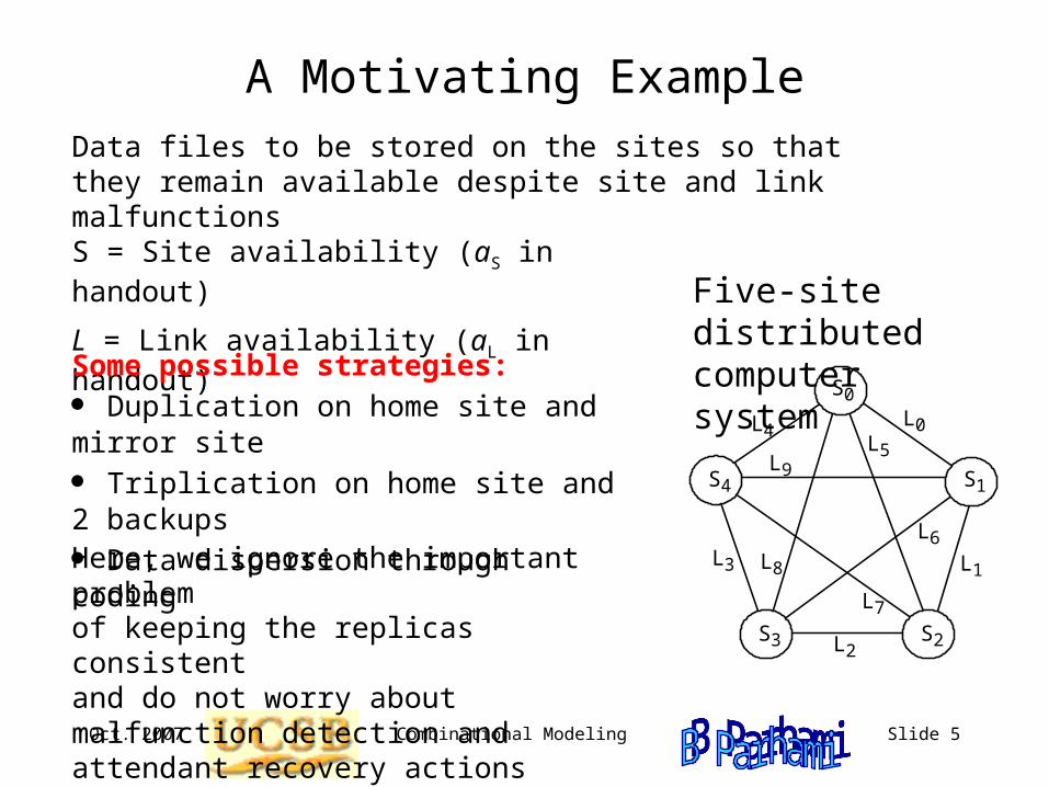
Five-site distributed computer system

Data files to be stored on the sites so that they remain available despite site and link malfunctions

S = Site availability (aS in handout)

L = Link availability (aL in handout)

Some possible strategies:

Duplication on home site and mirror site

Triplication on home site and 2 backups

Data dispersion through coding

Here, we ignore the important problem of keeping the replicas consistent and do not worry about malfunction detection and attendant recovery actions


Data Availability with Home and Mirror Sites

A = SL + (1 – SL)SL = 2SL – (SL)2

Requester

R

D

D

Home

Mirror

Assume data file must be obtained directly from a site that holds it

For example, S = 0.99, L = 0.95, A = 0.9965With no redundancy, A = 0.99 0.95 = 0.9405

Combinational modeling: Consider all combinations of circumstances that lead to availability/success (unavailability/failure)

R

D

D

R

D

D

R

D

D

R

D1 SL SL

SL 1 – L

(1 – S)LAnalysis by considering mutually exclusive subcases


Data Availability with TriplicationA = SL + (1 – SL)SL + (1 – SL)2SL = 3SL – 3(SL)2 + (SL)3

Requester

R

D

DD

Home

Backup 1

For example, S = 0.99, L = 0.95, A = 0.9998With duplication, A = 0.9965 With no redundancy, A = 0.9405

R

D

DD

R

D

D

R

D

DD

R

DD1

SL 1 – L

(1 – S)L

Backup 2

R

D

DD

R

D

DD

R

D

D

SL 1 – L (1 – S)L

1 SL SL

Can merge these two casesA = SL + (1 – SL) [SL + (1 – SL)SL]


Data Availability with File Dispersion

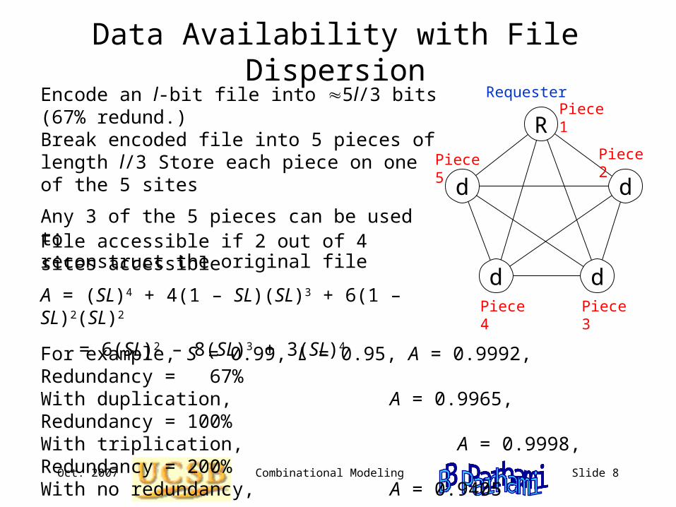
File accessible if 2 out of 4 sites accessible

A = (SL)4 + 4(1 – SL)(SL)3 + 6(1 – SL)2(SL)2

= 6(SL)2 – 8(SL)3 + 3(SL)4

Requester

R

d

dd

d

Piece 2

Encode an l-bit file into 5l/3 bits (67% redund.) Break encoded file into 5 pieces of length l/3 Store each piece on one of the 5 sites

Any 3 of the 5 pieces can be used to reconstruct the original file

Piece 1

Piece 4 Piece 3

Piece 5

For example, S = 0.99, L = 0.95, A = 0.9992, Redundancy = 67%With duplication, A = 0.9965, Redundancy = 100%With triplication, A = 0.9998, Redundancy = 200%With no redundancy, A = 0.9405


Series System

A system composed of n units all of which must be healthy for the system to function properly

R = Ri

Example: Redundant system ofvalves in series with regard to stuck-on-shut malfunctions (tolerates stuck-on-open valves)

Example: Redundant system of valves in parallel with regard to to stuck-on-open malfunctions (tolerates stuck-on-shut valves)


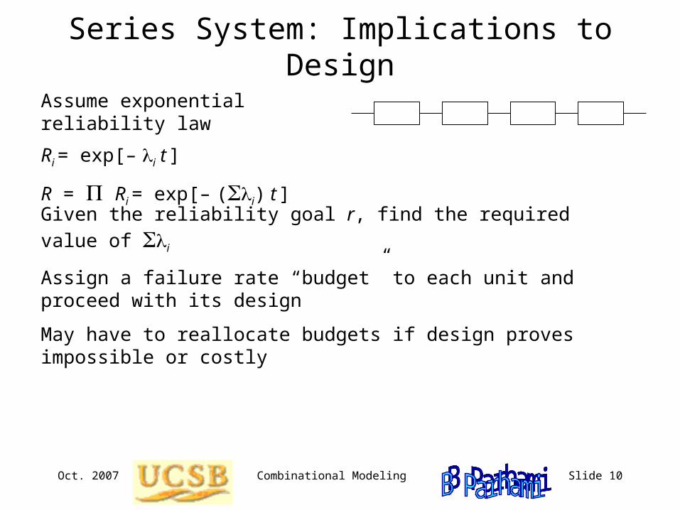
Series System: Implications to Design

Assume exponential reliability law

Ri = exp[– i t ]

R = Ri = exp[– (i) t ]

Given the reliability goal r, find the required value of i

Assign a failure rate “budget” to each unit and proceed with its design

May have to reallocate budgets if design proves impossible or costly


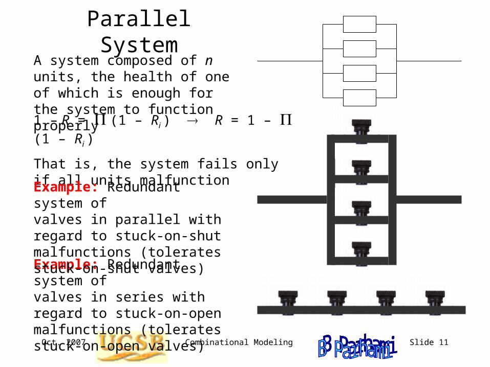
Parallel SystemA system composed of n units, the health of one of which is enough for the system to function properly

1 – R = (1 – Ri ) R = 1 – (1 – Ri )

That is, the system fails only if all units malfunction

Example: Redundant system of valves in series with regard to stuck-on-open malfunctions (tolerates stuck-on-open valves)

Example: Redundant system ofvalves in parallel with regard to stuck-on-shut malfunctions (tolerates stuck-on-shut valves)


Parallel System: Implications to Design

Assume exponential reliability law

Ri = exp[– i t ]

1 – R = (1 – Ri )

Given the reliability goal r, find the required value of 1 – r = (1 – Ri )

Assign a failure probability “budget” to each unit

For example, with identical units, 1 – Rm = n 1 – r

Assume r = 0.9999, n = 4 1 – Rm = 0.1 (module reliability must be 0.9)Conversely, for r = 0.9999 and Rm = 0.9, n = 4 is needed


The Concept of Coverage

For r = 0.9999 and Ri = 0.9, n = 4 is needed

Standby sparing: One unit works; others are also active concurrently or they may be inactive (spares)

When a malfunction of the main unit is detected, it is removed from service and an alternate unit is brought on-line; our analysis thus far assumes perfect malfunction detection and reconfiguration

R = 1 – (1 – Rm)n = Rm 1 – (1 – Rm)n

1 – (1 – Rm)

Let the probability of correct malfunction detection and successful reconfiguration be c (coverage factor, c < 1)

R = Rm See [Siew92], p. 2881 – cn(1 – Rm)n

1 – c(1 – Rm)


Impact of Coverage on System Reliability

Assume Rm = 0.95 Plot R as a function of n for c = 0.9, 0.95, 0.99, 0.999, 0.9999, 1

c: prob. of correct malfunction detection and successful reconfiguration

R = Rm 1 – cn(1 – Rm)n

1 – c(1 – Rm)

Unless c is near-perfect, adding more spares has no significant effect on reliability

In practice c is not a constant and may deteriorate with more spares; so too many spares may be detrimental to reliability

R

n2 4 8 16 32

0.9

0.99

0.999

0.9999

0.99999

0.999999

c = 0.9

c = 0.95

c = 0.99

c = 0.999

c = 1c = 0.9999


Series-Parallel SystemThe system functions properly if a string of healthy units connect one side of the diagram to the other

1 – R = (1 – R1 R2) (1 – R3 R4)

Example: Parallel connection of series pairs of valves (tolerates one stuck-on-shut and one stuck-on-open valve)

3

1

4

2

Example: Series connection of parallel pairs of valves (tolerates one stuck-on-shut and one stuck-on-open valve)

3

1

4

2

R = [1 – (1 – R1)(1 – R3)] [1 – (1 – R2)(1 – R4)]


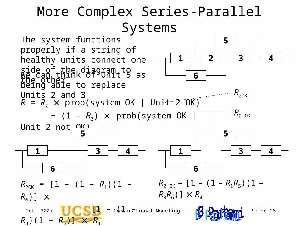
More Complex Series-Parallel SystemsThe system functions properly if a string of healthy units connect one side of the diagram to the other

R = R2 prob(system OK | Unit 2 OK)

+ (1 – R2) prob(system OK | Unit 2 not OK)

R2OK = [1 – (1 – R1)(1 – R6)]

[1 – (1 – R3)(1 – R5)]

R4

2 431

5

6We can think of Unit 5 as being able to replace Units 2 and 3

431

5

6

431

5

6

R2OK = [1 – (1 – R1R5)(1 – R3R6)] R4

R2OK

R2OK


Analysis Using Success Paths

R 1 – i(1 –Rith success path)

R 1 – (1 – R1R5R4) [*]

(1 – R1R2R3R4)(1 – R6R3R4)

2 431

5

6

This yields an upper bound on reliability because it considers the paths to be independent

2 431

5

6 43

1 4

With equal module reliabilities:

R 1 – (1 – Rm3)2 (1 – Rm

4)

If we expand [*] by multiplying out, removing any power for the various reliabilities, we get an exact reliability expressionR = 1 – (1 – R1R4R5)(1 – R3R4R6 – R1R2R3R4 – R1R2R3R4R6)

= R3R4R6 + R1R2R3R4 + R1R2R3R4R6 + R1R4R5 – R1R3R4R5R6

–R1R2R3R4R5 – R1R2R3R4R5R6 (Verify for the case of equal Rj )


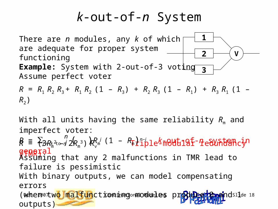
k-out-of-n System

There are n modules, any k of which are adequate for proper system functioning

V2

3

1

Example: System with 2-out-of-3 votingAssume perfect voter

R = R1 R2 R3 + R1 R2 (1 – R3) + R2 R3 (1 – R1) + R3 R1 (1 – R2)

With all units having the same reliability Rm and imperfect voter:

R = (3Rm2 – 2Rm

3) Rv Triple-modular redundancy (TMR)

R = j = k to n ( )Rmj (1 – Rm)n–j k-out-of-n system in general

nj

Assuming that any 2 malfunctions in TMR lead to failure is pessimisticWith binary outputs, we can model compensating errors (when two malfunctioning modules produce 0 and 1 outputs)


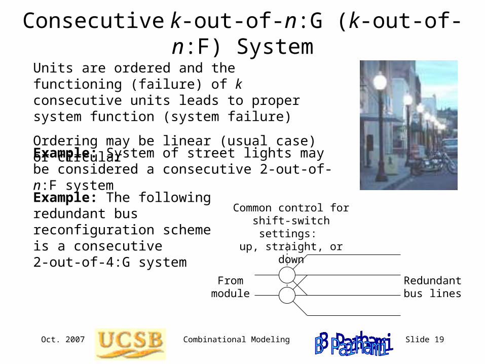
Consecutive k-out-of-n:G (k-out-of-n:F) System

Units are ordered and the functioning (failure) of k consecutive units leads to proper system function (system failure)

Ordering may be linear (usual case) or circular

Example: System of street lights may be considered a consecutive 2-out-of-n:F system

Example: The following redundant bus reconfiguration scheme is a consecutive 2-out-of-4:G system

From module

Redundant bus lines

Common control for shift-switch settings: up, straight, or down


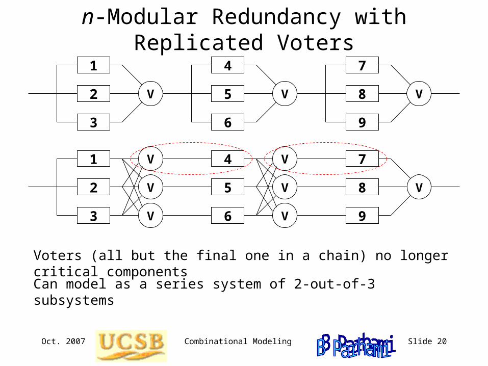
n-Modular Redundancy with Replicated Voters

Voters (all but the final one in a chain) no longer critical components

V2

3

1

V5

6

4

V8

9

7

V2

3

1

5

6

4

V8

9

7V

V

V

V

V

Can model as a series system of 2-out-of-3 subsystems


Fault Tree Analysis: Introduction

Quick guide to fault trees: http://www.weibull.com/basics/fault-tree/index.htm

Fault tree handbook: http://www.nrc.gov/reading-rm/doc-collections/nuregs/staff/sr0492/sr0492.pdf

Top-down approach to failure analysis:

Start at the top (tree root) with an undesirable event called a “top event” and then determine all the possible ways that the top event can occur

Analysis proceeds by determining how the top event can be caused by individual or combined lower-level undesirable events

Fault-tree tutorial: http://www.fault-tree.net/papers/dugan-comp-sys-fta-tutor.pdf

Example: Top event is “being late for work”Clock radio not turning on, family emergency, bus not running on timeClock radio won’t turn on if there is a power failure and battery is dead


Fault Tree Analysis: The Process

Basic events (leaf, atomic) Composite events

1. Identify “top event”

2. Identify 1st-level contributors to top event

3. Use logic gate to connect 1st level to top

4. Identify 2nd-level contributors

5. Link 2nd level to 1st level

AND gate

OR gate

Other symbols

XOR (not used

in reliability analysis)

k/n k-out-of-ngate

Externalevent

Enabling condition

Inhibitgate

6. Repeat until done


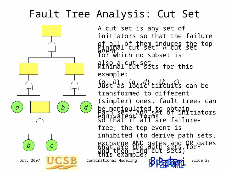
Fault Tree Analysis: Cut SetA cut set is any set of initiators so that the failure of all of them induces the top event

Minimal cut set: A cut set for which no subset is also a cut set

Minimal cut sets for this example:{a, b}, {a, d}, {b, c}

Just as logic circuits can be transformed to different (simpler) ones, fault trees can be manipulated to obtain equivalent forms

da b

cb

Path set: Any set of initiators so that if all are failure-free, the top event is inhibited (to derive path sets, exchange AND gates and OR gates and then find cut sets)

What are the path sets for this example?


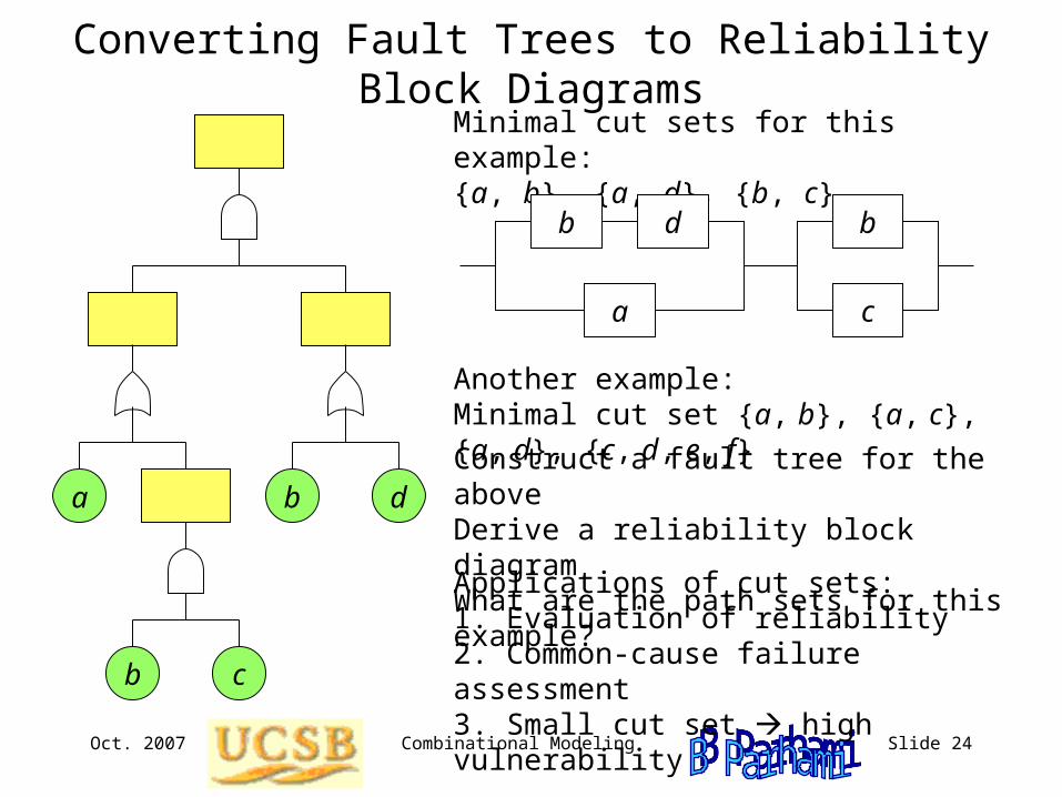
Converting Fault Trees to Reliability Block DiagramsMinimal cut sets for this example:{a, b}, {a, d}, {b, c}

Another example:Minimal cut set {a, b}, {a, c}, {a, d}, {c, d, e, f}

da b

cb

Construct a fault tree for the aboveDerive a reliability block diagramWhat are the path sets for this example?

Applications of cut sets:1. Evaluation of reliability2. Common-cause failure assessment3. Small cut set high vulnerability

b

a

d b

c

oct. 2007combinational modelingslide 1 fault-tolerant computing motivation, background, and tools

Documents

r d dd r d dd r d d

r d dd r d d r d dd

sl backup

sl analysis

requester r d dd d piece

requester r d d home

combinational modelingslide

requester r d dd home