odometry calibration and gait optimisationrobocup/2005site/reports05/robocup... · the university...
TRANSCRIPT

THE UNIVERSITY OF NEW SOUTH WALES
SCHOOL OF COMPUTER SCIENCE AND ENGINEERING
Odometry Calibration and Gait Optimisation
��������������
Submitted as a requirement for the degree
Bachelor of Software Engineering
Submitted: 23 September 2005
Supervisor: Dr. William Uther
Assessor: Professor Claude Sammut
The rUNSWift team is a joint project between the University of New South Wales and National ICT
Australia. National ICT Australia is funded through the Australian Government’s Backing Australia’s
Ability initiative, in part through the Australian Research Council.

- 1 -
Abstract
The locomotion module, which is responsible for handling the motion of the robot, is one of
the important modules in the robot architecture. This thesis will mainly concentrate two areas of improvements of the locomotion module: odometry calibration and gait optimisation.
Raised by significant changes of the RoboCup 4-Legged Leagued competition field, odometry calibrations are done much more accurately, with systematic methods and tools. A great portion of calibration methods are automatic.
Having a fast, stable gait is an important part in allowing legged robots to accomplish larger tasks. The automatic gait optimization process was based from rUNSWift’s previous work, yet has taken a large step by trying varies approaches, introducing new gait parameters, interpolating between optimised sets of gait parameters, to applying different learning algorithms. Offline analyse tools are also built to facilitate the process.

- 2 -
Acknowledgements Thank you to Alex, Nobuyuki, Josh and Andrew, the rUNSWift team, 2005. We had worked so hard yet enjoyed the greatest fun together. Thank you to Will, for your great insights and countless supports, and to Claude for your continuous guidance. Finally, thanks to Balint Seebar, who helped me on polishing this report.

- 3 -
Table of Contents:
Chapter 1: Introduction ....................................................................................... 6
1.1 Background........................................................................................... 7 1.2 Change of Competition Rules in 2005 ................................................... 8 1.3 rUNSWift System Architecture and Locomotion Module ...................... 9 1.4 Summary of Developments ................................................................. 10
Chapter 2: Odometry Calibration .......................................................................11
2.1 Problem Definition.............................................................................. 12 2.2 Related Work ...................................................................................... 12 2.3 Odometry Calibration Methods, 2005.................................................. 13
2.3.1 Data Gathering Process ................................................................ 14 2.3.2 Realisation Process....................................................................... 16
2.4 Evaluation........................................................................................... 19 2.5 Calibration for Special Actions............................................................ 20 2.6 Discussion........................................................................................... 20 2.7 Calibration Issues in the RoboCup 2005 Competition.......................... 21 2.8 Conclusion.......................................................................................... 22
Chapter 3: Gait Optimisation .............................................................................23
3.1 Introduction ........................................................................................ 24 3.2 Related Work ...................................................................................... 24 3.3 Gait Optimisation in 2005 ................................................................... 25 3.4 Gait Optimisation Method Details ....................................................... 26
3.4.1 The Process .................................................................................. 27 3.4.2 “Too Slow” Cases......................................................................... 28 3.4.3 More Discussion........................................................................... 29
3.5 Learning Algorithms ........................................................................... 30 3.5.1 Gradient Descent Method ............................................................. 31 3.5.2 Powell’s Method........................................................................... 31 3.5.3 Simplex Method ........................................................................... 32 3.5.4 Comparison.................................................................................. 33
3.6 Gait Parameters:.................................................................................. 35 3.6.1 Offline Actuator and Visualisation ................................................ 36 3.6.2 Common Gait Parameters............................................................. 37 3.6.3 Skelliptical Walk Specific Gait Parameters ................................... 39
3.7 Speed and Manoeuvrability ................................................................. 40 3.8 New Way of Walk Command Interpretation ........................................ 41 3.9 Walk Types Developed in 2005 ........................................................... 43
3.9.1 PG31 ............................................................................................ 44 3.9.2 PG22 ............................................................................................ 44 3.9.3 FastForward ................................................................................. 44 3.9.4 GrabDribble ................................................................................. 45

- 4 -
3.9.5 NeckTurnWalk ............................................................................. 46 3.10 Optimisation Issues in RoboCup 2005 Competition............................. 46 3.11 Conclusion: ......................................................................................... 47
Chapter 4: Behaviour .........................................................................................48
4.1 Early Developments of Best-Gap Finding ........................................... 49 4.2 Improved Ball Velocity Estimation...................................................... 50 4.3 Blocking Defence Skill ....................................................................... 51 4.4 Collision Detection ............................................................................. 52
Chapter 5: Conclusion .......................................................................................55
Appendix A..............................................................................................................58
Appendix B..............................................................................................................59
Appendix C..............................................................................................................61
Bibliography ............................................................................................................64

- 5 -
List of Figures:
Figure 1-1 The new look of the 2005 Competition field ...................................... 8 Figure 1-2 The rUNSWift system architecture []................................................. 9 Figure 2-1 A robot walks back and forth between landmarks for odometry
calibration................................................................................................. 13 Figure 2-2 Odometry calibration for sideways walking ..................................... 14 Figure 2-3 Odometry calibration for grab-turning ............................................. 14 Figure 2-4 Comparison of the best-fit quadratic function and the best-fit linear
function .................................................................................................... 18 Figure 2-5 Visual comparison of the official orange ball and the pink ball that
came with the original Aibo package......................................................... 22 Figure 3-1 Optimised Offset walk loci .............................................................. 24 Figure 3-2 Elliptical walk locus ........................................................................ 24 Figure 3-3 The training field for gait optimisation............................................. 26 Figure 3-4 Data flows between robot, base station and learning algorithm ........ 27 Figure 3-5 GUI of base station program for gait optimisation ........................... 29 Figure 3-6 Gradient descent method in 2D space .............................................. 31 Figure 3-7 Powell’s Method in 2D space, x’ is the conjugate direction vector.... 31 Figure 3-8 Simplex Method in 2D space ........................................................... 32 Figure 3-9 Visual comparison of Gradient descent method and Powell’s method
in a 2D search space, respectively. Powell’s method takes fewer steps to reach close to the minimum....................................................................... 33
Figure 3-10 The four leg walking loci of a newly developed minor walk type of Skelliptical walk ....................................................................................... 35
Figure 3-11 Effect of the walk loci with different gait parameters ..................... 37 Figure 3-12 Common Gait Parameters based on PWalk .................................... 37 Figure 3-13 The full set of Skelliptical Walk specific gait parameters ............... 39 Figure 3-14 Code segments for linear interpolation between 2 heights of front
legs. .......................................................................................................... 40 Figure 3-15 comparison of 2 set of leg loci in the horizontal plane, with both
large forward, left and turn commands. ..................................................... 42 Figure 3-16 code segment for turn walk calculation .......................................... 43 Figure 3-17 the FastForward standing stance .................................................... 45 Figure 3-18 the GrabDribble standing stance .................................................... 45 Figure 4-1 A processed CPlane image showing the gap finding......................... 50 Figure 4-2 Code Segments for subtract the robot’s movement from the last ball
position..................................................................................................... 51 Figure 4-3 The PWM readings of the robot leg joints when the robot walks
forward with a constant walk speed then collides with a wall. ................... 53 Figure 4-4 The irregular shapes of PWM reading during game play.................. 54

- 6 -
Chapter 1: Introduction
“By the year of 2050, a team of fully autonomous humanoid robot soccer players
shall win a soccer game, complying with the official rules of FIFA, against the winner
of the most recent World Cup.”
— RoboCup Federation
- 7 -
1.1 Background
RoboCup1 is an annual international competition held to motivate research into
artificial intelligence and robotics. By allowing direct comparison of complete robotic
systems through playing them in matches, RoboCup provides an effective test-bed for
a variety of robotic techniques. The ultimate goal of the RoboCup Federation is listed
as the quote of this chapter.
The RoboCup competition itself is divided into a variety of different leagues, in which
different types of robots compete. The RoboCup Four Legged League has a main
soccer tournament in which Sony ERS210 or ERS7 quadruped robots play soccer
against each other under modified soccer rules. No hardware modifications are
allowed in this league.
The rUNSWift team, a combined entry comprised of the University of New South
Wales (UNSW) and National ICT Australia (NICTA), has the greatest achievement
history in the RoboCup Four Legged League. rUNSWift has become world
champions three times (2000, 2001, 2003), achieved second place twice (1999, 2002)
and third this year, 2005.
In 2005, RoboCup was held at Intex Osaka in Osaka, Japan. Approximately 400 teams
from 35 countries participated in this competition, which attracted around 200,000
visitors.
1 RoboCup official website: http://www.robocup.org/
- 8 -
1.2 Change of Competition Rules in 2005
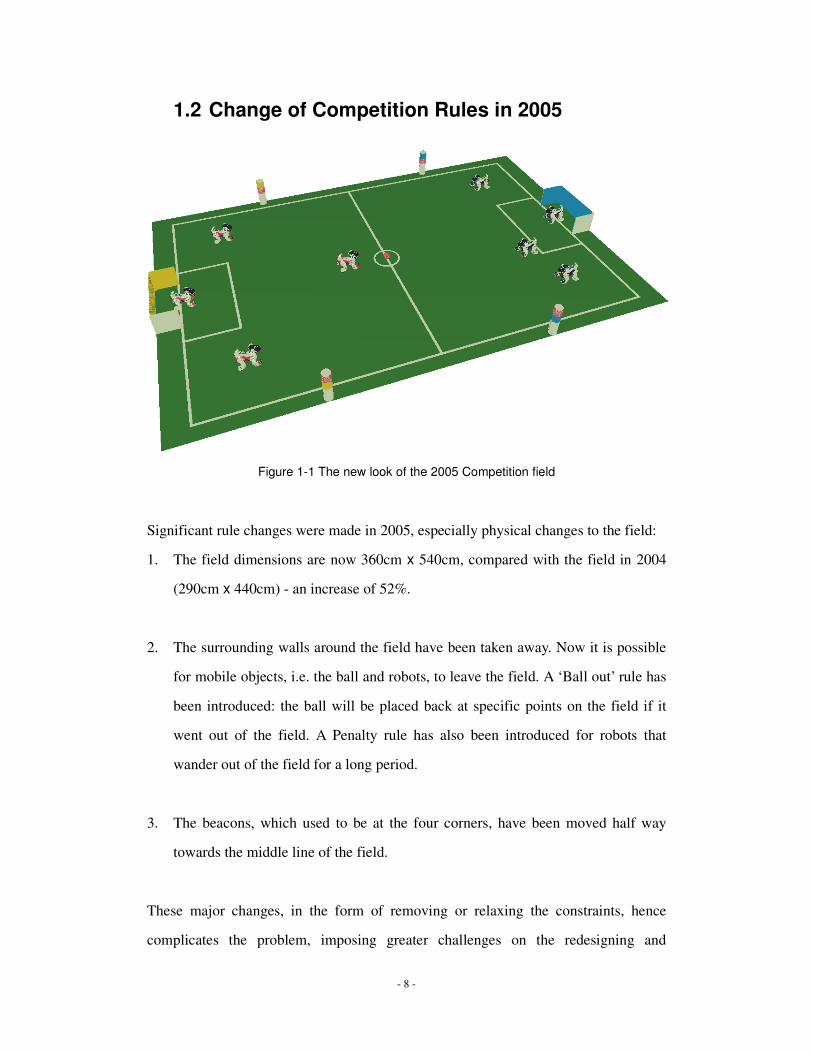
Figure 1-1 The new look of the 2005 Competition field
Significant rule changes were made in 2005, especially physical changes to the field:
1. The field dimensions are now 360cm x 540cm, compared with the field in 2004
(290cm x 440cm) - an increase of 52%.
2. The surrounding walls around the field have been taken away. Now it is possible
for mobile objects, i.e. the ball and robots, to leave the field. A ‘Ball out’ rule has
been introduced: the ball will be placed back at specific points on the field if it
went out of the field. A Penalty rule has also been introduced for robots that
wander out of the field for a long period.
3. The beacons, which used to be at the four corners, have been moved half way
towards the middle line of the field.
These major changes, in the form of removing or relaxing the constraints, hence
complicates the problem, imposing greater challenges on the redesigning and
- 9 -
implementation of the robot’s vision, localisation, locomotion and behaviour modules.
1.3 rUNSWift System Architecture and Locomotion
Module
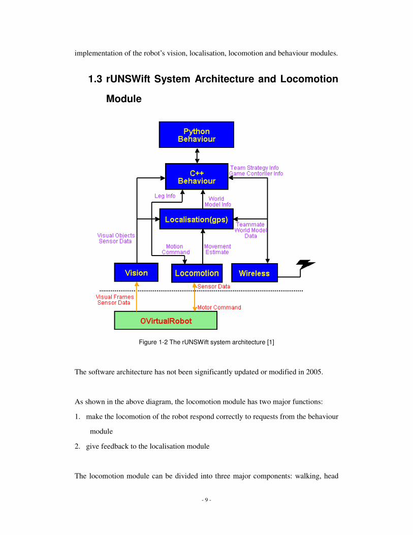
Figure 1-2 The rUNSWift system architecture [1]
The software architecture has not been significantly updated or modified in 2005.
As shown in the above diagram, the locomotion module has two major functions:
1. make the locomotion of the robot respond correctly to requests from the behaviour
module
2. give feedback to the localisation module
The locomotion module can be divided into three major components: walking, head

- 10 -
movement and special actions (kicking and blocking routines).
The behaviour module issues a set of walk commands to the locomotion module,
which consists of a major walk type, a minor walk type (the secondary walk type
within the major walk type), then the walking amounts in forward, left and turnCCW
(Turn in counter-clockwise direction) directions, in units of centimetres per walking
step, with negative values indicating going to the opposite direction.
1.4 Summary of Developments
The locomotion module, which is responsible for handling the motion of the
robot, is one of the important modules in the robot architecture. This thesis will
mainly concentrate two areas of improvements of the locomotion module: odometry
calibration and gait optimisation.
Raised by significant changes of the RoboCup 4-Legged Leagued competition
field, odometry calibrations are done much more accurately, with systematic methods
and tools. A great portion of calibration methods are automatic.
Having a fast, stable gait is an important part in allowing legged robots to
accomplish larger tasks. The automatic gait optimization process was based from
rUNSWift’s previous work, yet has taken a large step by trying varies approaches,
introducing new gait parameters, interpolating between optimised sets of gait
parameters, to applying different learning algorithms. Offline analyse tools are also
built to facilitate the process.
- 11 -
Chapter 2: Odometry Calibration
“What does the number 12 mean for Elliptical Walk?”
“It means its maximum forward speed.”
“What’s its unit? If I used 6, will the robot walk half of its maximum speed?”
“Umm... I’m not sure, I guess you can try it out…”
Wei Ming Chen, rUNSWift 2005 team member, and Kim Cuong Pham,
rUNSWift 2004 team member

- 12 -
2.1 Problem Definition
In order for the optimised locomotion system to be successful, it is important that
each locomotion strategy be correctly modelled.
In 2004, the walk commands issued from the behaviour module did not strictly
correlate with the actual locomotion of the robots (as illustrated in the quote of this
chapter). This wasn’t a big issue at that time, as the competition field was smaller and
landmarks (beacons and goals) could be more easily identified, as well as the robot
location. Also, with the help of the surrounding walls around the field, an attacking
strategy was simply to push the ball forward in the general direction of the target goal.
In 2005, the competition field has become larger, as mentioned in Section 1.2,
decreasing the chance of correct landmark identification, in turn creating the need for
more accurate internal odometry updates of the robot. This issue is also raised in the
situation where the robot tries to align itself with the largest gap of the goal (to where
it will kick the ball), which is considered important on the borderless field.
2.2 Related Work
Odometry calibration in the previous years of rUNSWift team was mainly done
manually. In 2005, the process has become automatic. The style for automatic
odometry calibration is very similar to the walk-learning systems introduced in 2003
[3]: a single robot walks back and forth between a pair of landmarks (beacons or
balls).
- 13 -
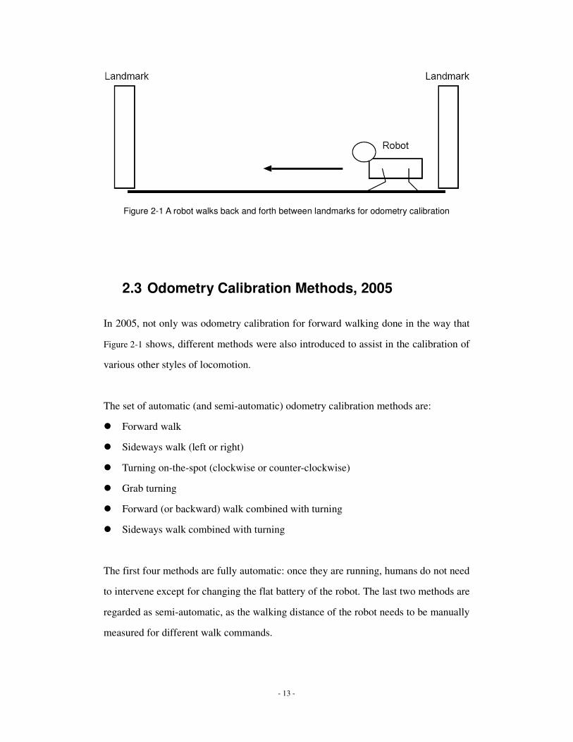
Figure 2-1 A robot walks back and forth between landmarks for odometry calibration
2.3 Odometry Calibration Methods, 2005
In 2005, not only was odometry calibration for forward walking done in the way that
Figure 2-1 shows, different methods were also introduced to assist in the calibration of
various other styles of locomotion.
The set of automatic (and semi-automatic) odometry calibration methods are:
� Forward walk
� Sideways walk (left or right)
� Turning on-the-spot (clockwise or counter-clockwise)
� Grab turning
� Forward (or backward) walk combined with turning
� Sideways walk combined with turning
The first four methods are fully automatic: once they are running, humans do not need
to intervene except for changing the flat battery of the robot. The last two methods are
regarded as semi-automatic, as the walking distance of the robot needs to be manually
measured for different walk commands.

- 14 -
All methods consist of two major components: a behaviour module, which runs on the
robot, and the base station program (named “walkBase”). The behaviour module
controls the robot’s locomotion and communicates with the base station, while the
base station receives and computes statistical data and issues new walk commands
when necessary.
All the methods also have 2 steps: data gathering and realisation. The data gathering
process varies between methods but the realisation is highly similar.
2.3.1 Data Gathering Process
To illustrate the data gathering process the sideways walking calibration method will
be used. Other methods share similar steps, and these differences will be discussed
afterwards.
Figure 2-2 Odometry calibration for sideways
walking
Figure 2-3 Odometry calibration for
grab-turning

- 15 -
As shown in Figure 2-2, odometry calibration for sideways walking has one
distinguished difference from forward walking: the robot points its head 90 degrees to
its body and walks sideways (left or right) between the beacons.
The robot first starts walking sideways towards one beacon from one end of another
beacon, always adjusting its heading by turning slightly to line up its head (not the
body) with its target. When one run is completed, i.e. the robot reaches the other end,
information is sent wirelessly to the base station containing the following:
� the elapsed time of that run
� raw (i.e. uncalibrated) walk command values (walk type / forward / left /
turnCCW)
The robot then turns around, walks back to the original target, sends out the same type
of information, and continues this process until the base station requests it to stop (or
its battery level becomes low).
The job of the base station program is to gather the elapsed time of 10-20 (adjustable)
runs from the robot for one particular set of walk commands, and then to find the
mean of them to determine the actual speed of the robot. Standard deviation of the
gathered data is used to eliminate outliners. A scheduler facilitates the calibration
process of different sets of walk commands automatically by testing them in
sequence.
To calibrate turning and grab-turning a somewhat different approach was used: the
robot turns on-the-spot, in either a clockwise or counter-clockwise direction, and uses
a stationary target, such as a ball on the ground, for taking time stamps, as shown in
Figure 2-3.
Combinations of calibrating forward walking and turning can also be made
semi-automatically. In such cases the robot will walk in a circle on the field (as a
- 16 -
result of combining constant turning). A stationary target can be used for time
stamping. Measuring the diameter of the circle can be used to calculate the forward
distance the robot walks; hence the actual forward speed and actual turn speed can be
calculated. This method can be used to combine walking backwards and turning, as
well as walking sideways and turning.
While the above calibration methods are done automatically or semi-automatically,
there is also an important manual calibration step that needs to be done: walking
backwards. The base station program issues walk commands to ask the robot to start
walking and then to stop, the walking distance of the robot is measured with a tape,
and finally this is entered manually into the base station program to calculate the
actual speed. Other manual calibration methods include grab-walking (except for grab
turning). These methods remain manual, because we could not find an effective
automatic process for them.
2.3.2 Realisation Process
After the data gathering process, the set of actual walking speeds of the robot with the
associated raw walk commands is obtained. A mathematical relation across this
association is needed so the locomotion module can make use of the data.
The actual speed values are plotted against the corresponding raw command values
once enough (typically 8-12) pairs of them are collected. A best-fit function F(r) = a,
where a is the actual speed value and r is the raw command value, is then found to
approximate the relation. Then the inverse function F’ of F needs to be found, the
reason being that when the high-level behaviour module requests a desired speed d,
the locomotion module needs to find a raw command value to make the actual speed a
match (i.e. d = a). As we know that F(r) = a, in order to find r, we need to calculate
F’(a), and since d = a, therefore r = F’(d).
- 17 -
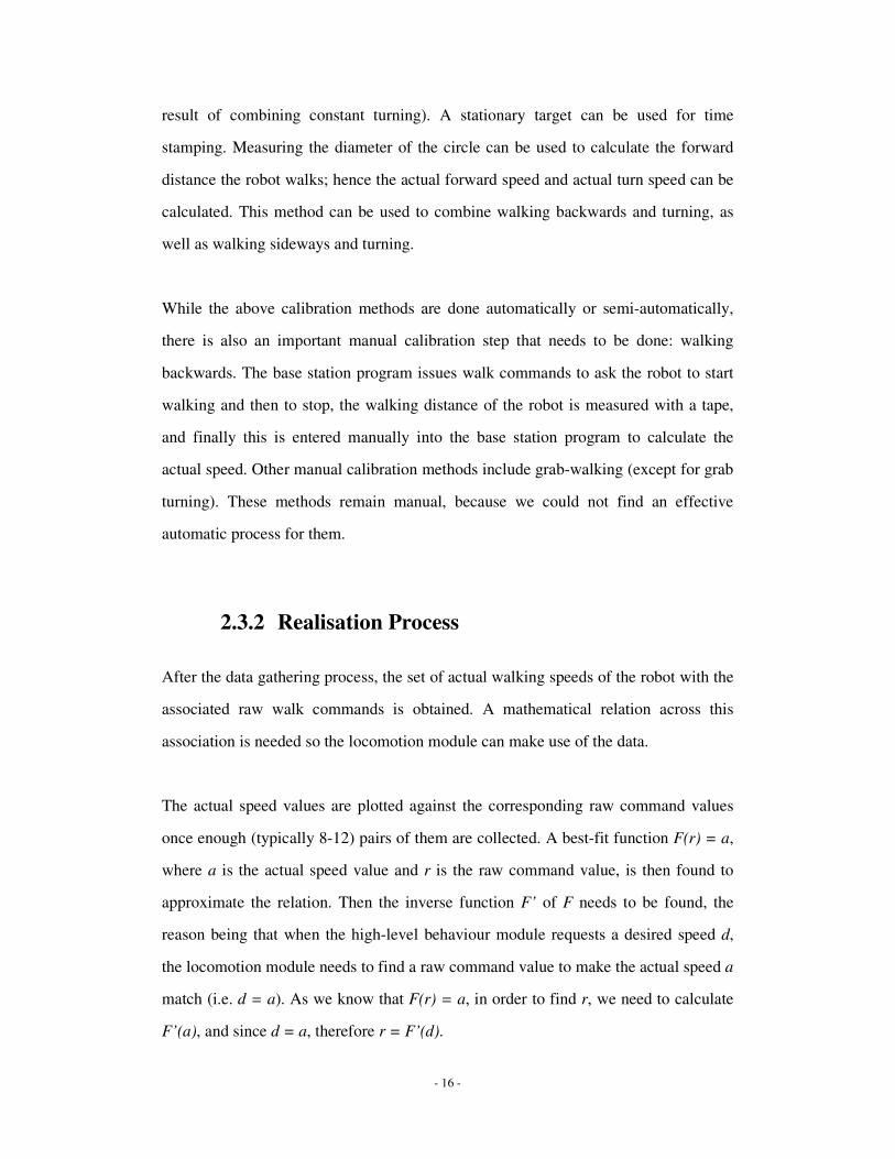
a = actual speed value
r = raw command value to reach the an actual speed ‘a’
F = best-fit function which represent the relationship of ‘a’ and ‘r’
F’ = inverse function of f
d = desired speed from behaviour module
)('
)(')(
dFr
ad
and
aFr
arF
=�
=
=�
=
When deciding the type of the best-fit function F, the observed trend of the
relationship shows that the actual speed increases as the raw commands increase,
however not quite in a linear fashion, and then drops in speed before reaching a peak
(its maximum or a minimum). After the peak, the actual speed starts to decrease with
even larger raw commands. From experimentation, a quadratic relation has indicated
a better approximation than a linear one, while still maintaining simplicity to find the
partial inverse function.

- 18 -
Figure 2-4 Comparison of the best-fit quadratic function and the best-fit linear function
After all the necessary calibrations are done for one type of walk and before applying
the results to the locomotion module, another form of calibrations is needed: small
corrections on the turning value to straighten pure forward and pure sideways walking.
This is due to the fact that centre of mass of the robot is not the centre of its body,
largely because of the heavy battery located in the left of the body. The robot will tend
to curve to the left or to the right when only a forward or sideways command is given.
The small corrections applied to the turning value in this case will make the robot
walk straight.
After all the calibration results are applied, the locomotion module is set up in a way
that the walk commands from behaviour module will be:
1. First, capped to maximum or minimum values as determined previously.
2. Then checked for special cases (i.e. if a combination of forward and turning is
- 19 -
used), and for them use the corresponding calibration results.
3. Or else, do a separate look-up in orthogonal directions and turning directions
4. Obtain the raw walk values from either step 2 or 3, and convert them, with the
gait parameters, to the joint angles of the robot (to control the locomotion).
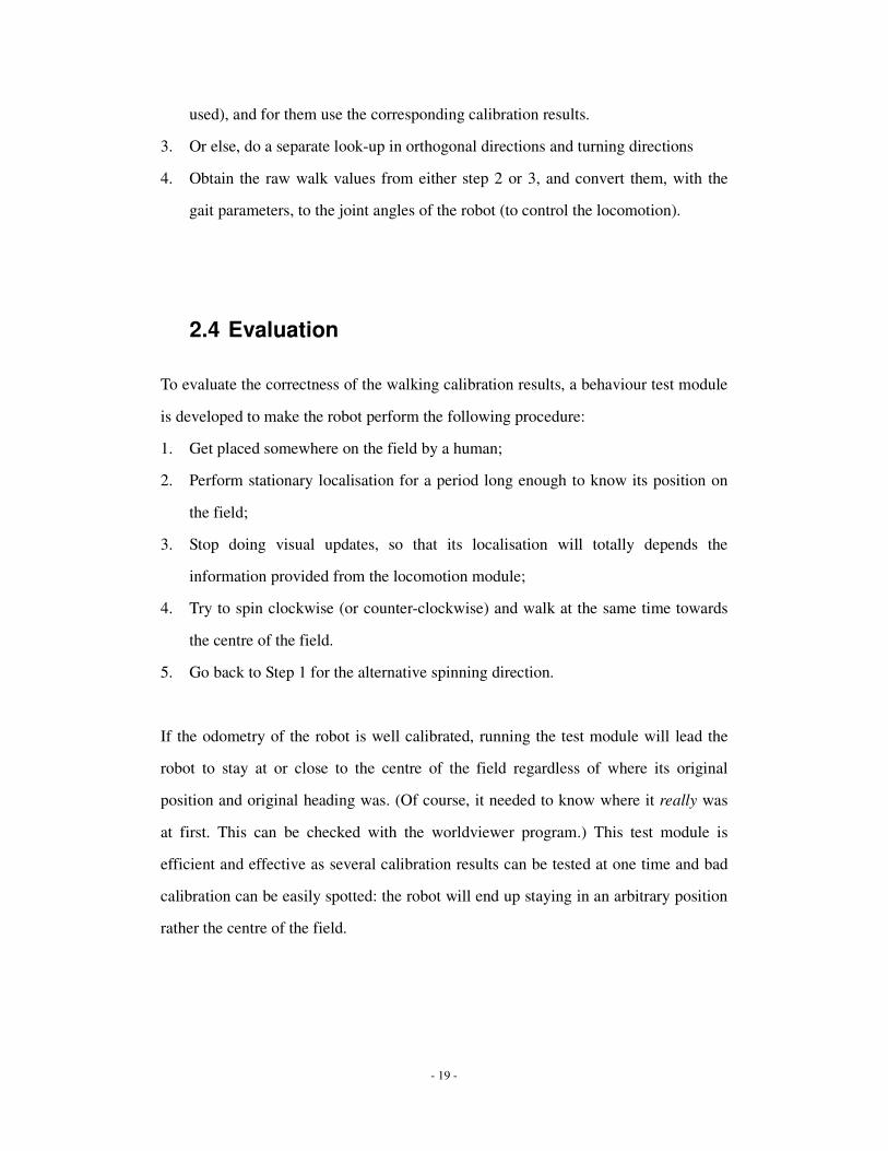
2.4 Evaluation
To evaluate the correctness of the walking calibration results, a behaviour test module
is developed to make the robot perform the following procedure:
1. Get placed somewhere on the field by a human;
2. Perform stationary localisation for a period long enough to know its position on
the field;
3. Stop doing visual updates, so that its localisation will totally depends the
information provided from the locomotion module;
4. Try to spin clockwise (or counter-clockwise) and walk at the same time towards
the centre of the field.
5. Go back to Step 1 for the alternative spinning direction.
If the odometry of the robot is well calibrated, running the test module will lead the
robot to stay at or close to the centre of the field regardless of where its original
position and original heading was. (Of course, it needed to know where it really was
at first. This can be checked with the worldviewer program.) This test module is
efficient and effective as several calibration results can be tested at one time and bad
calibration can be easily spotted: the robot will end up staying in an arbitrary position
rather the centre of the field.
- 20 -
2.5 Calibration for Special Actions
Apart from walking, the robot’s locomotion module is also responsible for performing
special actions. These special actions include various kicking and blocking routines.
In previous years of the rUNSWift team, the effect from the change of odometry after
performing a special action has been neglected, while in 2005, the effects were found
to be significant. For example, after performing a UPenn kick, the robot changes its
heading by 30 degrees; the robot will normally change its heading 10-20 degrees but
also move its position after performing a blocking action. These actions are now
calibrated.
2.6 Discussion
In a real game environment, arbitrary combinations of walk commands can be issued.
Since it is practically infeasible to calibrate all the possible combinations of walk
commands, our best effort is to calibrate in the orthogonal directions (forward,
backwards, left and right) as well as the turning directions (clockwise and
counter-clockwise). An overall effect is then assumed to be the combination of those
separately-calibrated directions.
In addition, it has been found that some combinations of walk commands (for
example, the robot walking forward combined with turning to get to the ball) are
favoured over others used from rUNSWift’s strategies. Therefore calibration methods
(e.g. forward and turning combined) are also especially developed for these
combinations.
Despite the fact that the automated odometry calibration methods have advantages,
they also have limitations:

- 21 -
� They typically required at least half of the field with two beacons standing
(turning calibration does not have this problem).
� Taking values of 10-20 runs for one set of walk commands is too time consuming,
as dozens of sets of walk commands are to be calibrated during the whole
calibration process.
2.7 Calibration Issues in the RoboCup 2005
Competition
In the world competition held in Osaka, Japan, even though we were one of the few
teams who were doing intensive odometry calibrations, there were still a lot of space
and time constraints, as 24 teams were using four fields to adapt to the environment in
two days.
Beacons cannot be used as time-stamping targets since that will take up half of the
field, and the field is normally shared between a couple of teams. A normal orange
competition ball, even though it can be placed anywhere on the field, is undesired
because there were simply too many other teams’ balls on the field at the same time.
To overcome these problems, we made the robot recognise a unique small pink ball
which originally comes with the Sony ERS7 Aibo package for the time-stamping
target. This is thanks to the new robust vision system developed this year by Alex
North[2] (one of the rUNSWift 2005 team members).

- 22 -
Figure 2-5 Visual comparison of the official orange ball and the pink ball that came with the
original Aibo package
Also to save time, we reduced the number of runs used for every set of walk
commands, or manual calibration was done altogether. Accuracy might have been
reduced as a trade off against the space and time constraints.
2.8 Conclusion
In this chapter, the need and reason for odometry calibration were shown. Various
new automatic calibration methods were compared. The full calibration process was
explained, as well as the evaluation methods. Issues with the RoboCup 2005
competition were also mentioned.
The odometry calibration, in practice, is never perfect, due to its complex nature.
However, we have achieved better odometry than that of previous years by means of
introducing new automated odometry calibration methods and more careful
considerations of the different aspects of the problem.
- 23 -
Chapter 3: Gait Optimisation
“Whoever gets to the ball first is who dominates the game.”
“Manoeuvrability is just as important as speed.”
Claude Sammut, Co-supervisor of rUNSWift 2005 team

- 24 -
3.1 Introduction
It is clear that effective gaits have a significant impact on the overall effectiveness of
legged robots in most environments. A fast and stable gait is also important in the
context of game play.
Gait optimisation, especially automatic gait optimisation, has been developed by the
rUNSWift team since 2003 and has been adopted by other teams around the world
very quickly. Machine learnt gaits are faster and more stable than hand tuned ones.
The new Sony robot model ERS7, introduced in 2004, has more powerful leg joints
than the old model ERS210, hence the maximum walking speed has been increasing.
3.2 Related Work
rUNSWift, as the first team who used the automatic gait optimisation technique,
developed the fastest walk on the Sony ERS210 model during 2003[3]. Members Min
Sub Kim and Will Uther developed an offset walk, which can achieve a maximum
forward speed at a mean of 27cm/sec.
Figure 3-1 Optimised Offset walk loci
Figure 3-2 Elliptical walk locus

- 25 -
In 2004, this work was continued with the new Sony ERS7 model by Kim Cuong
Pham [4], by applying a gradient descent method. This resulted in an optimised walk
with an elliptical walk locus, which achieved a maximum forward speed of 34cm/sec.
Similar work includes Austin Villa [5], which shares a lot of common ideas with
rUNSWift, yet has its own features: their walk was not locus-based and a genetic
algorithm was used. Reasonable achievements have been reported.
3.3 Gait Optimisation in 2005
In 2005, based on rUNSWift’s previous years’ experiences, more tools and methods
were developed to facilitate the process of gait optimisation. Various approaches have
been tested, from introducing new gait parameters, interpolating between optimised
sets of gait parameters, to applying different learning algorithms. We also visually
represented the gait loci offline to analyse and compare the results of using different
sets of gait parameters. A new training field (rather than the normal competition field)
was constructed; therefore intensive “walk training” could be performed without
interfering with the behavioural development for game play.

- 26 -
Figure 3-3 The training field for gait optimisation
One of the achievements in 2005 is the maximum forward speed on the ERS7 model.
It has increased to 43cm/second, a 26% of improvements compared with the year
2004. Another positive result is the increase in the manoeuvrability of the robot – a
direct outcome from the more comprehensive automatic gait optimisation.
3.4 Gait Optimisation Method Details
This section will describe the general details of the 2005 gait optimisation method.
Specific details such as learning algorithms will be described in Section 3.5 and
details of gait parameters will be described in Section 3.6 .
The robot behaviour for automatic gait optimisation is similar to the odometry
calibration method in Section 2.3: the robot walks between two targets with a certain
set of gait parameters, measures the walking time, and sends it back to the same base
station program. The difference is that there is a learning algorithm using this
information to generate new sets of gait parameters.
- 27 -
For data collection the same base station program is used. However, to evaluate one
set of gait parameters, only the results from four runs are used, in contrast with the
10-20 results odometry calibration required. The reason for this is there are a large
amount of combinations of gait parameters even when they are discretised. Therefore
we want to be quick so as to try out as many sets of parameters as possible.
A trial of gait optimisation is one unique test for finding the optimised set of gait
parameters, starting from an initial predefined set. In a typical trial, more than 100
sets of gait parameters are tested, each has an evaluation value for certain sets of gait
parameters based on the timing of the four runs of the robot.
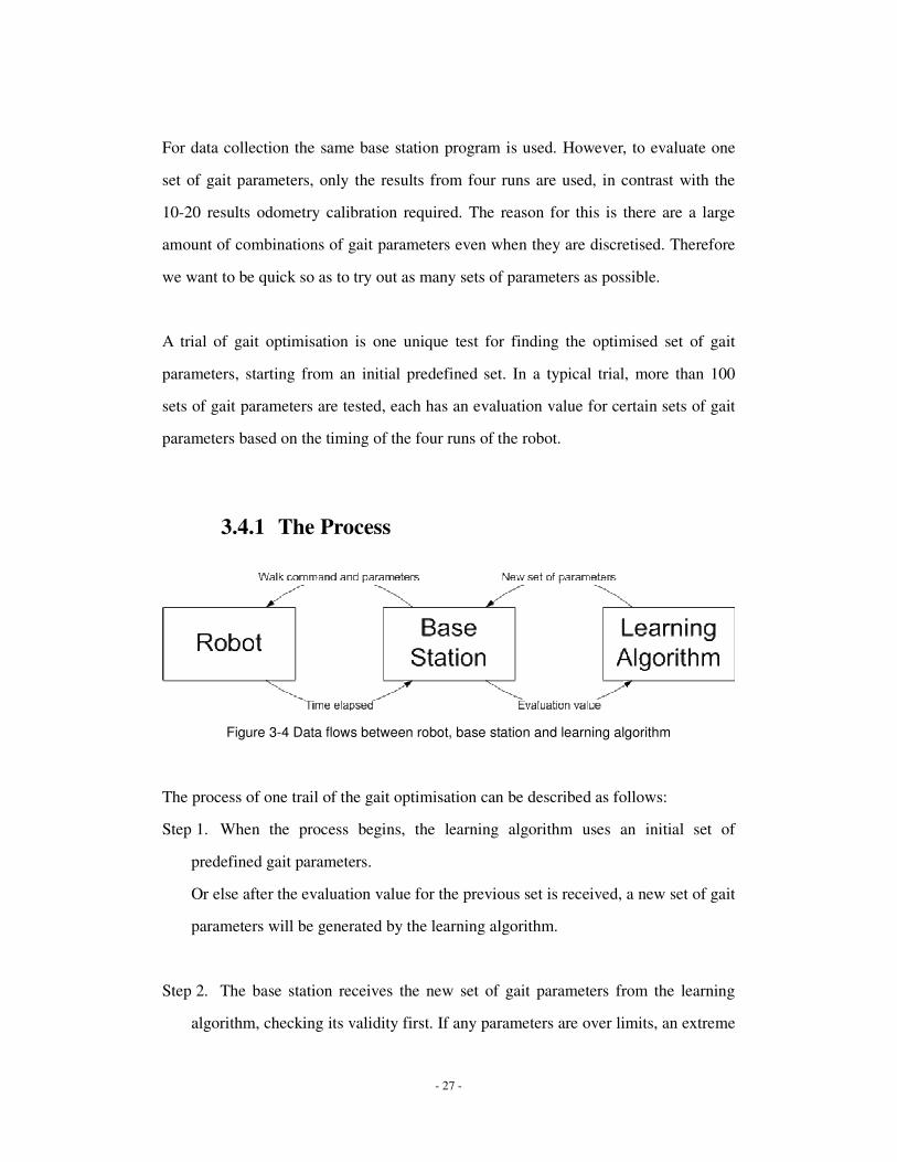
3.4.1 The Process
Figure 3-4 Data flows between robot, base station and learning algorithm
The process of one trail of the gait optimisation can be described as follows:
Step 1. When the process begins, the learning algorithm uses an initial set of
predefined gait parameters.
Or else after the evaluation value for the previous set is received, a new set of gait
parameters will be generated by the learning algorithm.
Step 2. The base station receives the new set of gait parameters from the learning
algorithm, checking its validity first. If any parameters are over limits, an extreme

- 28 -
evaluation value will be sent back to the learning algorithm, and it will go back to
Step 1.
Or else the gait parameters will be sent along with other necessary walk
commands to the robot.
Step 3. The robot then follows the commands, walks between targets, and sends back
the elapsed time as the result of that run.
Step 4. The base station waits until results of four runs are received. The evaluation
value of that set of gait parameters is then calculated by taking the median value
of the four results, i.e. throwing away the highest and lowest results and
averaging the middle two. This is then sent to the learning algorithm. Then Step 1
repeated.
There are notes for each step:
For Step 1: Very different set of gait parameters are used for the initial set in order to
explore the search space more broadly. Alternatively, the optimised set from a former
trail can be used for the purpose to (hopefully) optimise it further.
For Step 2: Depending on the nature of the learning algorithm, the extreme evaluation
values can be ‘infinity’ (an extremely large number) for gradient insensitive
algorithms, or a reasonable large number (twice or five times the longest elapsed time)
for gradient sensitive algorithms.
For Step 3 and Step 4: A full four runs may not be executed, as human intervention is
required in some cases, and will be discussed in the below section.
3.4.2 “Too Slow” Cases
During the optimisation process, some combinations of gait parameters may make the
robot walk in a very slow fashion, or barely walk at all. In such cases, human

- 29 -
interventions are required.
� The first case is moderate: if the set of gait parameters make the walk speed of
the robot low, and a much faster result has been gained already, the results of 1 or
2 runs are sufficient, and the process can move on to the next set;
� The second case is more extreme: the set of gait parameters makes robot barely
walk, or even walk in the opposite direction, so either a reasonably large number
or ‘infinity’ is used for the results of that set, depending on the chosen learning
algorithm.
3.4.3 More Discussion
Figure 3-5 GUI of base station program for gait optimisation
During the whole optimisation process, the base station program performs the

- 30 -
following functions:
� Bridge: as the robot does not know there is a learning algorithm, and the learning
algorithm does not know the nature of the problem (i.e. the search space), the
base station links the two to make the optimisation take place smoothly.
� Storage: it stores and can retrieve later sets of optimised gait parameters and
evaluated values for previous parameter sets.
� Monitoring: the user can see the history and current state, and can also intervene
or analyse the progress of automatic gait optimisation.
Also, the learning algorithms do not know about the constraints on the gait parameters,
therefore it is the base station’s job to ensure the next set of generated gait parameters
is valid: a set of gait parameters with any off-limit values are immediately evaluated
as extreme.
Moreover, the learning algorithms assume the search space is continuous, while some
gait parameters are discretised (such as PG, the number of control points in a half-step)
and so are rounded off to the nearest valid value.
3.5 Learning Algorithms
In 2005, three different learning algorithms were investigated and compared. They are
all function minimisation methods: normal gradient descent method, Powell’s method
and Simplex method. This section gives brief review rather than the mathematical
details, along with practical comparisons, in the gait optimisation context.
- 31 -
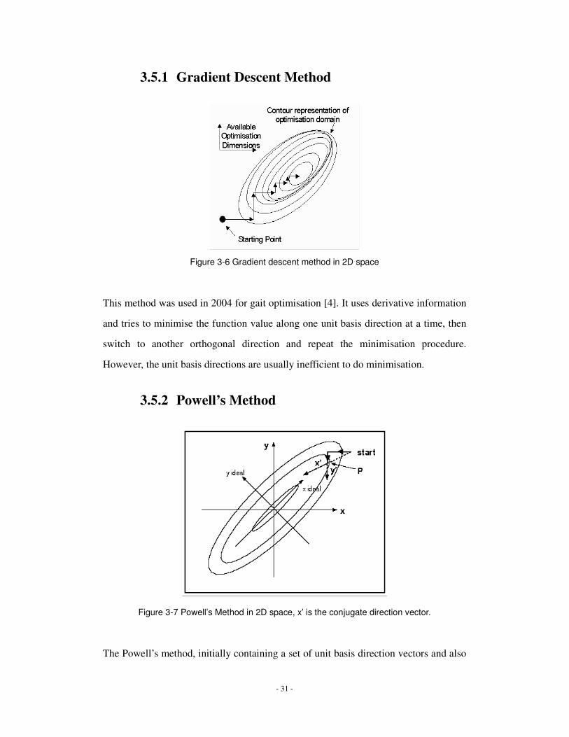
3.5.1 Gradient Descent Method
Figure 3-6 Gradient descent method in 2D space
This method was used in 2004 for gait optimisation [4]. It uses derivative information
and tries to minimise the function value along one unit basis direction at a time, then
switch to another orthogonal direction and repeat the minimisation procedure.
However, the unit basis directions are usually inefficient to do minimisation.
3.5.2 Powell’s Method
Figure 3-7 Powell’s Method in 2D space, x’ is the conjugate direction vector.
The Powell’s method, initially containing a set of unit basis direction vectors and also

- 32 -
using derivative information, runs like the gradient descent approach on the first run.
However, it then works out a conjugate direction, which is a better direction rather
than orthogonal ones, and replaces a ‘poor’ one in the set, and then continues the
process.
Due to the long time required for function evaluation, we also modify the general
Powell’s method to speed it up by:
1) Limiting the line search: the number of function evaluations on one dimension is
limited to 3-5.
2) Saving the direction vectors and reusing them during the next trail.
3) Using the changed (usually non-orthogonal direction) vector first, so that more
gait parameters can be changed.
3.5.3 Simplex Method
Figure 3-8 Simplex Method in 2D space2
The simplex method, rather than depending on the use of gradients, uses a
2 Figure from http://es1.ph.man.ac.uk/AJM2/e2e/param/param.htm

- 33 -
geometrical figure - the simplex, consisting of N+1 vertices in N-dimensions of the
search space. It then applies various transformations (reflection, expansion,
contraction) to roll the simplex “downhill” toward the minimum.
3.5.4 Comparison
Figure 3-9 Visual comparison of Gradient descent method and Powell’s method in a 2D search
space, respectively. Powell’s method takes fewer steps to reach close to the minimum3
Theoretically, Powell’s method and the simplex method will perform better than the
gradient descent method, and this was proven from software simulations as well as
actual practice on gait optimising of the robots.
While the software simulation indicates that Powell’s method and the simplex method
have no advantages over each other, practical results show that the simplex method
outperforms Powell’s method in the use of gait optimisation for the same amount of
time.
This is largely due to the nature of the gait optimisation problem:
3 Figure from http://math.fullerton.edu/mathews/n2003/powellmethod/PowellMethodMod/Links/PowellMethodMod_lnk_8.html

- 34 -
� The time taken for function evaluation is long: The robot has to run back and
forth four times between two targets to calculate the median time. This takes
about 30-40 seconds to evaluate one set of gait parameters.
� The search space is large: the number of gait parameters are about 20-30, which
means the search space is in 20-30 dimensions!
It is also due to the nature of the algorithms themselves:
� The “setup” time of the two algorithms differs: Powell’s method needs to do
3-5 function evaluations along each unit basis direction before it can come up
with a better direction to continue in. With a large search space like our gait
optimisation, the number of function evaluations for “setting-up” is also large:
70-150. As the simplex method only needs to examine each unit basis direction
once to constructing the simplex, it is then able to roll downhill immediately.
� The extent of exploring the search space: if not all unit basis direction vectors
are replaced by the direction set in Powell’s method, it is likely that the algorithm
will change only the value of one parameter in the gait parameter set, hence not
exploring the search space thoroughly. The simplex method, on the other hand,
with the transformations it performs on the simplex, normally changes the values
of the whole gait parameter set and so is considered to explore the search space
more broadly.
If the optimisation process is run long enough, it is possible for Powell’s method to
catch up with the simplex method. However, the practical nature of gait optimisation
prefers a faster solution. (In fact, the legs of a couple of robots have been broken
during the gait optimisation process. It may or may not have been caused by the
long-hour running of the robots.)
- 35 -
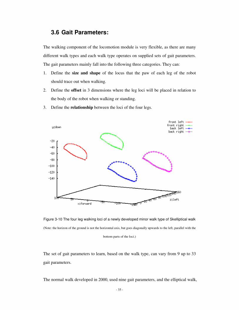
3.6 Gait Parameters:
The walking component of the locomotion module is very flexible, as there are many
different walk types and each walk type operates on supplied sets of gait parameters.
The gait parameters mainly fall into the following three categories. They can:
1. Define the size and shape of the locus that the paw of each leg of the robot
should trace out when walking.
2. Define the offset in 3 dimensions where the leg loci will be placed in relation to
the body of the robot when walking or standing.
3. Define the relationship between the loci of the four legs.
Figure 3-10 The four leg walking loci of a newly developed minor walk type of Skelliptical walk
(Note: the horizon of the ground is not the horizontal axis, but goes diagonally upwards to the left, parallel with the
bottom parts of the loci.)
The set of gait parameters to learn, based on the walk type, can vary from 9 up to 33
gait parameters.
The normal walk developed in 2000, used nine gait parameters, and the elliptical walk,

- 36 -
which was developed in 2004, has four extra. The Skelliptical walk, which was also
developed in 2004, but only saw intensive use in 2005, uses 22 extra gait parameters,
putting the total number of learnable gait parameters to 33. The set of gait parameters
for the Skelliptical walk has been investigated in depth with the aid of specially
designed tools.
By analysing the gait parameters, not only does the team have a better understanding
of them, the team can decide whether the current set of gait parameters are sufficient,
or to select the important gait parameters to optimise first.
3.6.1 Offline Actuator and Visualisation
Part of the locomotion module can be run offline (i.e. not in the robot) step by step to
reproduce the walking loci of the robot. ‘Offline Actuator’ is such a program, in
combination with a Linux plotting program ‘gnuplot’, which can visually display the
leg loci for a set of walk commands and gait parameters. Figure 3-10 is one of the
examples. Figure 3-11 shows the effects of different gait parameters on the leg loci:
a b
c d

- 37 -
e f
Figure 3-11 Effect of the walk loci with different gait parameters
a) normal loci, b) PG = 5, c) canter = 8, d) frontDutyCycle = 70, e) frontLiftUpHeight = 5, f) thrustH=30
3.6.2 Common Gait Parameters
All rUNSWift walk types are direct subclasses or derivations of the class PWalk,
developed in 2000. Therefore there is a set of common gait parameters shared
between walk types. There are 9 of them.
Figure 3-12 Common Gait Parameters based on PWalk
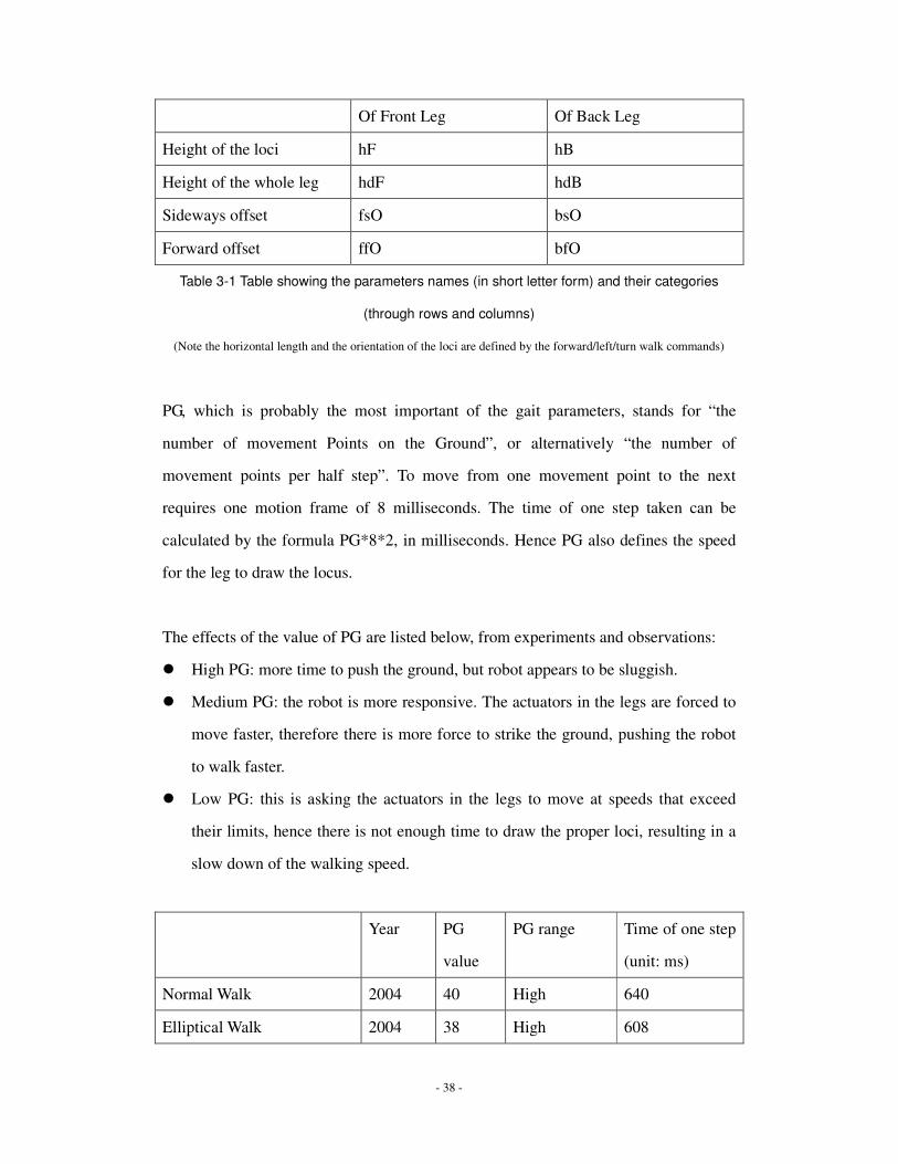
8 common parameters are used to define the heights and offsets of the loci:
- 38 -
Of Front Leg Of Back Leg
Height of the loci hF hB
Height of the whole leg hdF hdB
Sideways offset fsO bsO
Forward offset ffO bfO
Table 3-1 Table showing the parameters names (in short letter form) and their categories
(through rows and columns)
(Note the horizontal length and the orientation of the loci are defined by the forward/left/turn walk commands)
PG, which is probably the most important of the gait parameters, stands for “the
number of movement Points on the Ground”, or alternatively “the number of
movement points per half step”. To move from one movement point to the next
requires one motion frame of 8 milliseconds. The time of one step taken can be
calculated by the formula PG*8*2, in milliseconds. Hence PG also defines the speed
for the leg to draw the locus.
The effects of the value of PG are listed below, from experiments and observations:
� High PG: more time to push the ground, but robot appears to be sluggish.
� Medium PG: the robot is more responsive. The actuators in the legs are forced to
move faster, therefore there is more force to strike the ground, pushing the robot
to walk faster.
� Low PG: this is asking the actuators in the legs to move at speeds that exceed
their limits, hence there is not enough time to draw the proper loci, resulting in a
slow down of the walking speed.
Year PG
value
PG range Time of one step
(unit: ms)
Normal Walk 2004 40 High 640
Elliptical Walk 2004 38 High 608
- 39 -
Skelliptical Walk (PG31) 2005 31 Medium 496
Skelliptical Walk
(FastForward)
2005 23 Medium 368
Table 3-2 Comparison of PG values between 2004 and 2005 walk types
In 2005, all the common gait parameters were considered important and therefore
were all machine learnt.
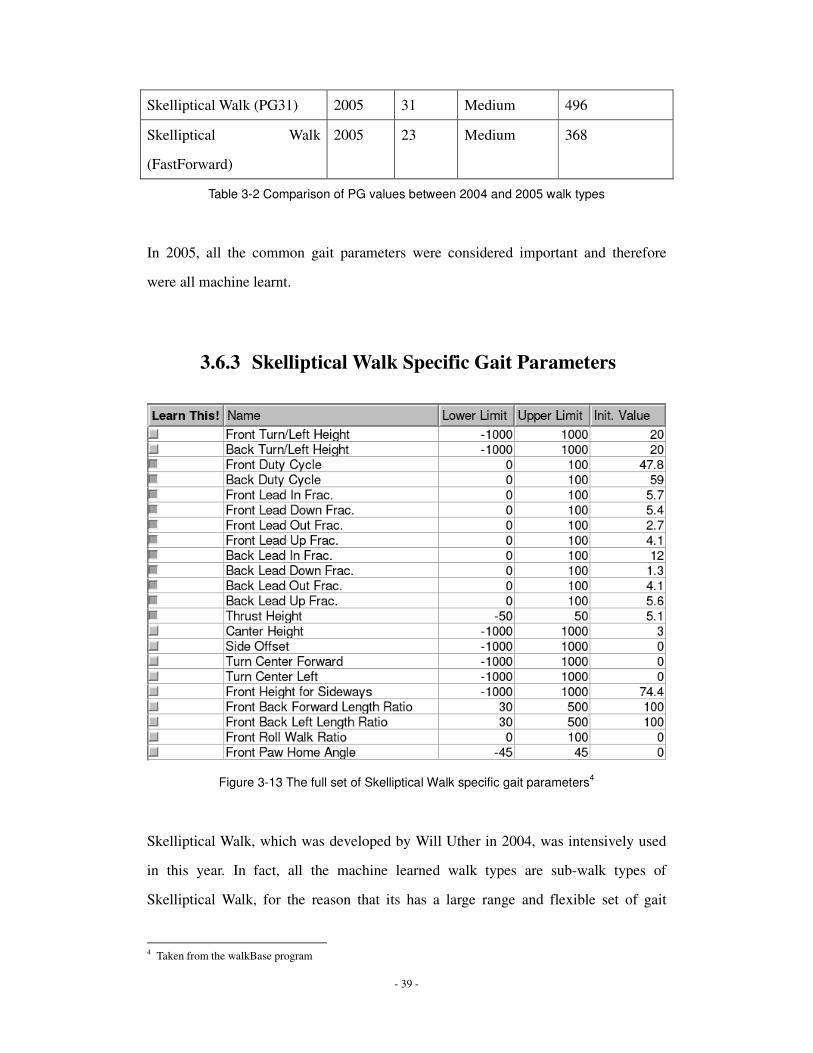
3.6.3 Skelliptical Walk Specific Gait Parameters
Figure 3-13 The full set of Skelliptical Walk specific gait parameters4
Skelliptical Walk, which was developed by Will Uther in 2004, was intensively used
in this year. In fact, all the machine learned walk types are sub-walk types of
Skelliptical Walk, for the reason that its has a large range and flexible set of gait
4 Taken from the walkBase program

- 40 -
parameters. There are a total of 22.
For a detailed description and usage of each gait parameters, please refer to the
comments in the source code (SkellipticalWalk.h and SkellipticalWalk.cc) of
Skelliptical Walk provided in the Appendix A and Appendix B.
Example Parameter: Front Height for Sideways
This is a newly introduced gait parameter in 2005. An observation is that a tilted robot
body (low front, high back) will make the robot works forward faster, while a flat
body (equal front and back height) makes the sideways walking faster.
Therefore this parameter is introduced to cope with the sideways case, while hF is
used for forward walking. Linear interpolation is make between hF and this parameter
according to values of a given walk commands, as shown in the below code segment:
void SkellipticalWalk::setFrontH() {
// setting the front Height according to walk commands
// also sets all other attributes depends on front Height
double frontHMix;
if (stepParms.cmdFwd == 0 && stepParms.cmdLeft == 0)
frontHMix = 1;
else {
frontHMix = fabs(stepParms.cmdFwd) /
(fabs(stepParms.cmdFwd) + fabs(stepParms.cmdLeft));
}
frontH = frontHMix * walkParms.frontH + (1-frontHMix) * walkParms.frontLeftH;
Figure 3-14 Code segments for linear interpolation between 2 heights of front legs.
3.7 Speed and Manoeuvrability
As one of the quote from this chapter “Manoeuvrability is just as important as speed.”
by Professor Claude Sammut, we don’t just consider the maximum (forward) speed of

- 41 -
the robot alone.
In 2004, 2 separate walk types Normal Walk and Elliptical Walk are used to
comprehend speed and manoeuvrability: whenever speed (especially forward speed)
is required, Elliptical Walk is used, while manoeuvrability is required, the slower
Normal Walk is then used.
In 2005, similar strategy was used, except that later one only one walk was used, as it
has the fastest forward speed as well as is most manoeuvrable among all the learned
walks.
We have described the automatic gait optimisation method for finding the fast forward
walk in Section 3.4. However, finding a fast yet manoeuvrable walk can also been
done in a similar fashion. This time the base station will instruct the robot not only to
walk forward for 4 runs, but also to use the same set of gait parameters to walk
backwards, walk to the left, walk to the right, turn in clockwise direction and turn in
counter clockwise direction, all for 4 runs separately. Then the median elapsed time is
found for each set of 4 runs, and sum up to be the final evaluation value.
3.8 New Way of Walk Command Interpretation
Apart from automatic optimisation on gait parameters, we also find a potential better
way to interpret the walk commands from the behaviour module. Related work has
been developed by the German team in 2004 [6].
When combining the large values of forward, left and turnCCW commands together,
they generally do not perform the same way as expected. Especially when there is
forward and left one direction and turning to another direction (e.g. forward
- 42 -
10cm/step, left 10cm/step, turning clockwise 40degrees/step). In 2004, to overcome
this issue, the behaviour module caps the values to while performing combinations of
walk commands. This is undesired as it has not used the full potentials of the robot’s
locomotion.
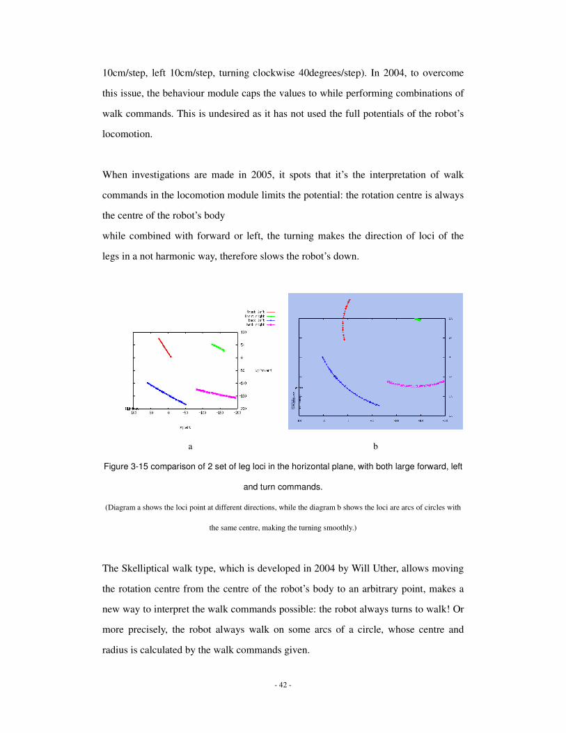
When investigations are made in 2005, it spots that it’s the interpretation of walk
commands in the locomotion module limits the potential: the rotation centre is always
the centre of the robot’s body
while combined with forward or left, the turning makes the direction of loci of the
legs in a not harmonic way, therefore slows the robot’s down.
a
b
Figure 3-15 comparison of 2 set of leg loci in the horizontal plane, with both large forward, left
and turn commands.
(Diagram a shows the loci point at different directions, while the diagram b shows the loci are arcs of circles with
the same centre, making the turning smoothly.)
The Skelliptical walk type, which is developed in 2004 by Will Uther, allows moving
the rotation centre from the centre of the robot’s body to an arbitrary point, makes a
new way to interpret the walk commands possible: the robot always turns to walk! Or
more precisely, the robot always walk on some arcs of a circle, whose centre and
radius is calculated by the walk commands given.

- 43 -
The below code segment show the calculation. Variables cmdFwd, cmdLeft and
cmdTurn are the walk commands given from the behaviour module. The code results
in changing turnLen as well as walkParms.turnCenterF and
walkParms.turnCenterL, which is the position of the circle.
double dist = sqrt(cmdFwd * cmdFwd + cmdLeft * cmdLeft);
dist = CLIP(dist, 21.0); // assume it's our step limit in cm.
turnLen = DEG2RAD(cmdTurn);
double radius = dist / tan(turnLen);
double thetaTangent = atan2(cmdLeft, cmdFwd);
walkParms.turnCenterF = -radius * sin(thetaTangent) * 10;
walkParms.turnCenterL = radius * cos(thetaTangent) * 10;
turnLen = turnLen * 1; // <- calibration goes here
fwdLen = leftLen = 0
Figure 3-16 code segment for turn walk calculation
However, due to time constraint and the difficulty for odometry calibration, the new
way of interpreting the walk commands was not used in the game play.
3.9 Walk Types Developed in 2005
There are quite a few new walk types introduced in 2005, some of them are machine
learned (optimised) and the others are the derivations of the optimised walk types for
- 44 -
special purposes.
All of them are essential Skelliptical walk type, with different set of gait parameters.
In this section, we will briefly explain the feature of each of the new walk types
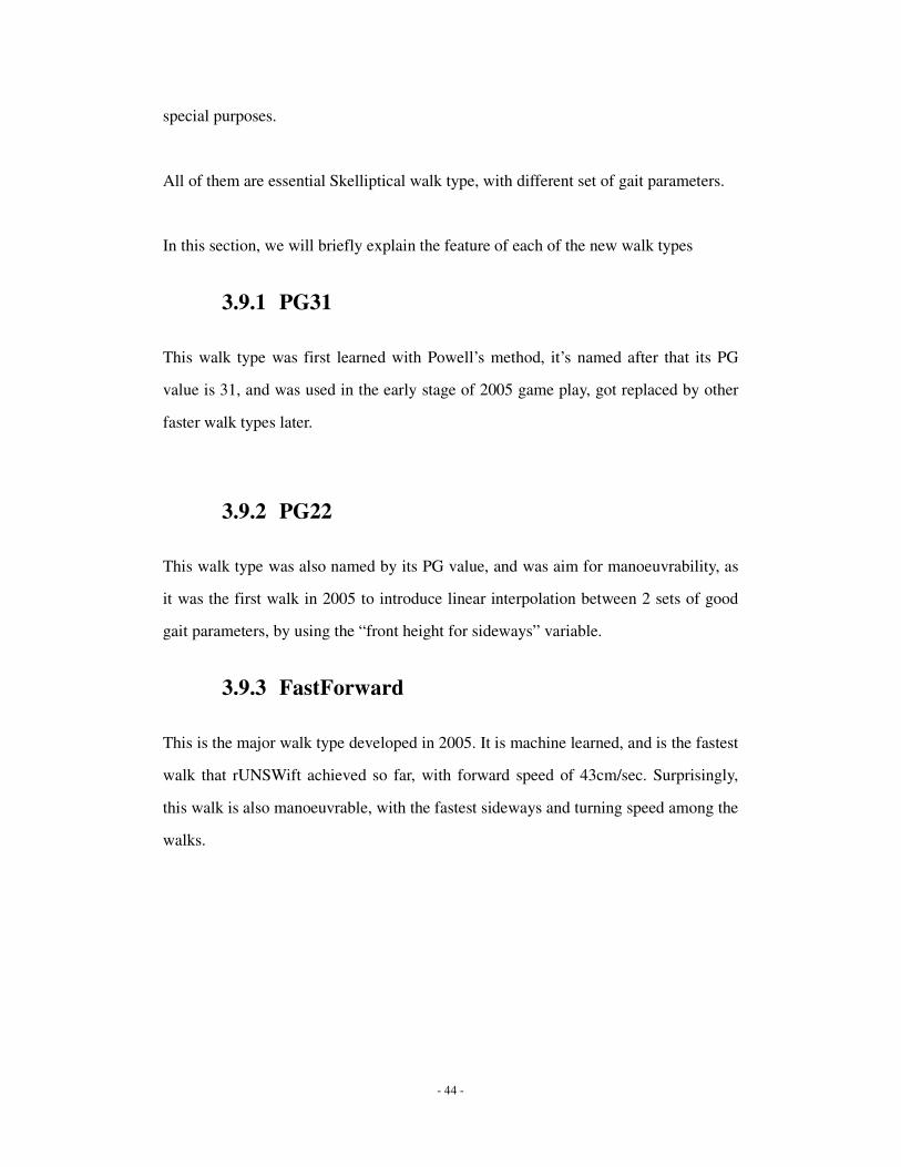
3.9.1 PG31
This walk type was first learned with Powell’s method, it’s named after that its PG
value is 31, and was used in the early stage of 2005 game play, got replaced by other
faster walk types later.
3.9.2 PG22
This walk type was also named by its PG value, and was aim for manoeuvrability, as
it was the first walk in 2005 to introduce linear interpolation between 2 sets of good
gait parameters, by using the “front height for sideways” variable.
3.9.3 FastForward
This is the major walk type developed in 2005. It is machine learned, and is the fastest
walk that rUNSWift achieved so far, with forward speed of 43cm/sec. Surprisingly,
this walk is also manoeuvrable, with the fastest sideways and turning speed among the
walks.

- 45 -
Figure 3-17 the FastForward standing stance
For this walk type, the back legs of the robot stick up, making the robot’s body tilted;
the front knees bend to their maximum most of the time, that the front legs act like
wheels rolling on the ground while the robot walks forwards.
3.9.4 GrabDribble
Figure 3-18 the GrabDribble standing stance
- 46 -
This walk type is based on the FastForward walk type, except that the front legs has
rotated a bit more forward, to give more protection to the ball, preventing the ball to
slip out when the robot is walking with this walk type.
3.9.5 NeckTurnWalk
This walk type is also based on the FastForward walk type, with the only change that
the rotation centre has moved from the centre of the body to the neck of robot. This
walk type is used for close to ball line up behaviours.
3.10 Optimisation Issues in RoboCup 2005
Competition
The carpets of the competition fields of RoboCup 2005, were thicker and softer than
the carpet on rUNSWift’s practice field. The “front rolling wheel” property of
FastForward walk type had experience frictions on the thick carpet in Osaka,
suffering a 10% speed decrement.
A new faster forward walk were quickly learned on the field, however, the new walk
was not so manoeuvrable as the FastForward walk and also as FastForward being too
integrated into behaviour, it would require a great deal of effects on making changes
to adapt the new walk. We decided to sacrifice some speed for manoeuvrability, as the
ball close up behaviours required.
Through the preliminary games, it was ok, as our walking speed normally
overwhelmed the opponent’s. However, in the semi-final match against the Nubots
team, This, turned out, trading speed for manoeuvrability was an inappropriate

- 47 -
decision: it’s our first time to appeared to walk a little bit slower than the opponent
team, hence less chance to control the ball, or got control of the ball with opponents
nearby most of the time.
3.11 Conclusion:
In 2005, there was surely a big practical achievement on gait optimisation, as the
maximum forward speed of the robot has increased by a large amount to 43 cm/sec, at
the same time the walk of the robot has also gain manoeuvrability. The work to
achieve this result was based rUNSWift team’s previous experiences, along with
trying different approaches to attack the problem.
Even though 3 different learning algorithms were tried and analysed, there are yet
other feasible learning algorithms to be investigated and tested, named: genetic
algorithm and simulated annealing, as they are believed will explore the search space
more broadly.
Also, there are lessons learned:
1. The proposed optimised walk should be tested on different carpets to prevent
“over optimisation” on one particular kind of carpet.
2. More careful consideration should be made when there is a trade-off between
speed and manoeuvrability.
- 48 -
Chapter 4: Behaviour
“Let’s challenge Nobu’s so-called aggressive attacker with a defensive goalie.”
“Alright.”
Wei Ming Chen and Josh Shammay, rUNSWift 2005 team members

- 49 -
4.1 Early Developments of Best-Gap Finding
An attacking robot (with the ball) relies on the vision system to estimate the distance
and heading to the goal, and tries to aim to the goal to score.
However, just aiming to the goal is not enough, because most of the time, there will
be an opponent goalie robot (and often other robots) standing between the goal and
the attack robot, hence finding the largest open gap of the goal to shoot is a better
option.
In previous years, the best-gap finding method is based on recognising the size of the
goalie robot and other robots, however, the new Sony ERS-7 robot model is much
harder to recognise and so other approaches have been used.
While the colour blobbing vision system was still in use, the best-gap finding method
does a thin horizontal line scanning over the area just below the middle of the visual
goal object in the colour plane (CPlane), comparing the number of goal colour pixels
to judge the largest gap of the goal.
In Figure 4-1 A processed CPlane image showing the gap finding, the goal is divided
into 2 gaps (between red lines and between yellow lines) by the blue goalie. The
attacking robot will then try to shoot to the larger gap rather than blindly shooting to
the middle of the goal, where the blue goalie is standing.

- 50 -
Figure 4-1 A processed CPlane image showing the gap finding
With the new vision system using horizontal line scanning to recognise the goal,
picking the longest horizontal lines in the bottom region of the goal as the best gap
suffices.
4.2 Improved Ball Velocity Estimation
In previous years, the rUNSWift code calculated the ball velocity by getting the local
ball positions in consecutive frames, finding the difference in each pair of them in the
x and y directions, averaging them and then using that as the estimated ball velocity.
However, this method has two major flaws:
1. It does not take into count the movements of the robots when calculating the
difference of ball positions
2. It does not have good tolerance for occasionally missing visual ball information in
some frames, the most important information is the ball local position.

- 51 -
In 2005, we particularly subtract the movements of the robot from previous ball local
position, so that previous ball position is expressed in the current robot’s position’s
coordinates, as expressed in the following code segment:
void KI2DWithVelocity::shiftLastBallPos(double dForward, double dLeft, double dTurn) {
// we need to inverse the movements to get the last correct ball local pos
Vector pos(vCART, lastx - dForward, lasty + dLeft); // right is positive
pos.rotate(-dTurn);
lastx = pos.getX();
lasty = pos.getY();
}
Figure 4-2 Code Segments for subtract the robot’s movement from the last ball position
For occasionally missing visual ball, we keep track of the number of missing frames,
until the ball is reacquired, then we use the this formula to calculate the ball velocity:
Ball vel = (current ball pos – last visual ball pos) / (#missing frames + 1)
The combination of these 2 solutions, has been proved to improved ball velocity
estimation.
4.3 Blocking Defence Skill
Based on the new and more reliable ball velocity calculations, new behaviours can be
developed with the advantage of predicting future ball locations. Blocking is one of
them.
There are three different kinds of blocking special actions in the locomotion module,
all originally developed by The German Team:
� Middle Blocking: the robot stretch both of its two front legs to each side,

- 52 -
� Left Blocking: the robot moves its body to the left and stretches its left front leg
sideways to its maximum limit
� Right Blocking: the robot moves its body to the right and stretches its right front
leg sideways to its maximum limits
A behaviour module is developed to decide under what situation to block, or not to.
Source code of that module is in Appendix C.
Blocking is considered to be a very important strategy of the Goalie, as well as for the
defender and supporter roles. For the attacker role, we decided not use blocking
because the first priority of an attacker is to get to the ball as quickly as possible.
4.4 Collision Detection
The Locomotion module also can give feedbacks of its joint sensors’ information to
the behaviour module. Each leg has 3 actuators, and each actuator has 2 read out – the
sensor value and the PWM value, given a total amount of 2 x 3 x 4 = 24 different
values. By carefully analyse those values, collision detection of the robot can be done
with a simple environment, Figure 4.3 shows such a case. The Nubot team, also have
done related work by comparing the actual sensor values with the expected values. [7]
- 53 -
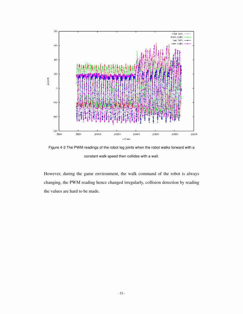
Figure 4-3 The PWM readings of the robot leg joints when the robot walks forward with a
constant walk speed then collides with a wall.
However, during the game environment, the walk command of the robot is always
changing, the PWM reading hence changed irregularly, collision detection by reading
the values are hard to be made.
- 54 -
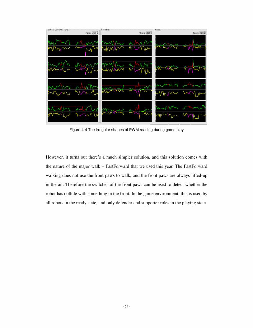
Figure 4-4 The irregular shapes of PWM reading during game play
However, it turns out there’s a much simpler solution, and this solution comes with
the nature of the major walk – FastForward that we used this year. The FastForward
walking does not use the front paws to walk, and the front paws are always lifted-up
in the air. Therefore the switches of the front paws can be used to detect whether the
robot has collide with something in the front. In the game environment, this is used by
all robots in the ready state, and only defender and supporter roles in the playing state.

- 55 -
Chapter 5: Conclusion
“I always have these kinds of off-stage feelings after the world competition each
year.”
Will Uther, Supervisor of rUNSWift 2005 team

- 56 -
The RoboCup 2005 Competition, was finished on 17th of July, 2005. The rUNSWift
team has reclaimed its top positions in the world, as achieved the third place in the
competition. This was due to significant improvements over different modules of the
rUNSWift software system. The locomotion module, was one of them.
The major improvements on the locomotion module can be summarised to the
following two sentences:
1. The locomotion of the robot has responded to the request of the behaviour
module more accurately.
2. The locomotion of the robot has become more responsive and more competent.
The first improvement was directly raised the strategies designed to cope with the
physical changes of the competition field, as much more accurate robot behaviours
are required on a larger, borderless field. The re-pickup of best-gap goal shooting
strategy also required great deal of accuracy from the locomotion.
Systematic and intensive odometry calibrations, automatically or semi-automatically
were developed for such needs. Varies automatic methods were introduced and
developed. Methodologies were built up and the calibration process got speeded up
over time. Previous neglected area (calibration for special action) were noticed and
improved. Frequent walking patterns (forward with turning only) were also
discovered and special calibrations were done for them.
However, the odometry calibration can never be perfect, due to its complex nature.
Smaller amount of walking will take longer time to calibrate and will get more
affected by other factors. However, we were confident that better odometry has been
obtained than previous years by the mean of systematic odometry calibration methods
and more careful considerations of the different aspects of the problem.
The second improvement of locomotion module, is driven by a continued yet more
- 57 -
comprehensive work of gait optimisation. Experiences on the importance of a fast and
stable gait in the game play pushed the optimisation forwards. Efforts and resources
were transfused. A new training ground was built up solely for the purpose of gait
optimisation, or walk learning. The learning process has been developed highly
automatically and possibilities for speed-up were sought. Learning algorithms were
compared and modified. Gait parameters and leg loci were studied intensively.
Moreover, new possible way to improve the gait (in the form of new gair parameters)
has come out frequently.
And the results were satisfactory: A 26% improvement on the maximum forward
speed to 43cm/second, the robot became more responsive, and manoeuvrability had
also been achieved.
However, there are deficiency and places for further improvement for gait
optimisation:
� The optimised gait was “too optimised” on one type of the ground, should be
tested more on different type of surface.
� Other learning algorithms such as genetic algorithms, can be investigated.
� The walk command interpretation is possible to be improved
Overall, the improvements of the locomotion module were satisfactory, Combinations
of improvements with other modules, have made the rUNSWift 2005 team a strong
and competent team.

- 58 -
Appendix A
Gait Parameter definitions in Skelliptical Walk: class skelWalkParms { public: int halfStepTime; // the number of points (8ms apart) in half a step double frontFwdHeight; // the height off the ground of the front leg recovery when moving forward double frontTrnLftHeight; // the height off the ground of the front leg recovery when moving sideways/turning double backFwdHeight; // the height off the ground of the back leg recovery when moving forward double backTrnLftHeight; // the height off the ground of the back leg recovery when moving sideways/turning double frontDutyCycle; // the percentage (0-1) of the step that the front feet are on the ground double backDutyCycle; // the percentage (0-1) of the step that the back feet are on the ground double frontLeadInFrac; // the percentage (0-1) of the first half of the ground stroke that is 'lead in' for the front legs double frontLeadDownFrac; // the percentage (0-1) of the recovery height that is 'lead in' for the front legs double frontLeadOutFrac; // the percentage (0-1) of the second half of the ground stroke that is 'lead out' for the front legs double frontLeadUpFrac; // the percentage (0-1) of the recovery height that is 'lead out' for the front legs double backLeadInFrac; // the percentage (0-1) of the first half of the ground stroke that is 'lead in' for the back legs double backLeadDownFrac; // the percentage (0-1) of the recovery height that is 'lead in' for the back legs double backLeadOutFrac; // the percentage (0-1) of the second half of the ground stroke that is 'lead out' for the back legs double backLeadUpFrac; // the percentage (0-1) of the recovery height that is 'lead out' for the back legs double frontF; // the distance forward from the shoulder of the home point of the front legs double frontS; // the distance sideways from the shoulder of the home point of the front legs double frontH; // the vertical distance from the shoulder of the home point of the front legs (when walking forward) double frontLeftH; // the vertical distance from the shoulder of the home point of the front legs (when walking sideways) double backF; // the distance forward from the shoulder of the home point of the back legs double backS; // the distance sideways from the shoulder of the home point of the back legs double backH; // the vertical distance from the shoulder of the home point of the back legs double sideOffset; // a left/right offset to move the center of balance double turnCenterF; // a front/back adjustment to the centre of turn double turnCenterL; // a left/right adjustment to the centre of turn double frontBackForwardRatio; // an adjustment to the forward distance travelled by the front legs relative to the back legs (to account for slip) double frontBackLeftRatio; // an adjustment to the sideways distance travelled by the front legs relative to the back legs (to account for slip) double frontHomeAngleDeg; // the angle in degrees of the home point on the front lower leg double frontRollWalkRatio; // the amount of rolling vs. walking that the front leg should do. 0 == all walk, 1 == all roll double thrustHeight; double canterHeight;

- 59 -
Appendix B
Gait Parameter usages in Skelliptical Walk: void SkellipticalWalk::setFrontH() { // setting the front Height according to walk commands // also sets all other attributes depends on front Height double frontHMix; if (stepParms.cmdFwd == 0 && stepParms.cmdLeft == 0) frontHMix = 1; else { frontHMix = fabs(stepParms.cmdFwd) / (fabs(stepParms.cmdFwd) + fabs(stepParms.cmdLeft)); } frontH = frontHMix * walkParms.frontH + (1-frontHMix) * walkParms.frontLeftH; bodyTilt = asin((walkParms.backH - frontH)/lsh); shoulderDist = lsh*cos(bodyTilt); double dF = shoulderDist/2; double dS = BODY_WIDTH/2; flFOffset = dF + walkParms.frontF - walkParms.turnCenterF; flLOffset = -dS - walkParms.frontS + walkParms.turnCenterL + walkParms.sideOffset; flTheta0 = atan2(flFOffset, flLOffset); flRadius = sqrt(flFOffset*flFOffset + flLOffset*flLOffset); frFOffset = dF + walkParms.frontF - walkParms.turnCenterF; frLOffset = dS + walkParms.frontS + walkParms.turnCenterL + walkParms.sideOffset; frTheta0 = atan2(frFOffset, frLOffset); frRadius = sqrt(frFOffset*frFOffset + frLOffset*frLOffset); blFOffset = -dF + walkParms.backF - walkParms.turnCenterF; blLOffset = -dS - walkParms.backS + walkParms.turnCenterL + walkParms.sideOffset; blTheta0 = atan2(blFOffset, blLOffset); blRadius = sqrt(blFOffset*blFOffset + blLOffset*blLOffset); brFOffset = -dF + walkParms.backF - walkParms.turnCenterF; brLOffset = dS + walkParms.backS + walkParms.turnCenterL + walkParms.sideOffset; brTheta0 = atan2(brFOffset, brLOffset); brRadius = sqrt(brFOffset*brFOffset + brLOffset*brLOffset);
}
void SkellipticalWalk::setStepParams(const struct skelStepParms &newParms) { stepParms = newParms; double oldTime = time; double oldStep = step; time = 2*walkParms.halfStepTime*stepParms.shortStep; if (time < 1) { // stop a whole lot of problems with div by 0 // You can't do anything in zero or -ve time time = 1; standing = true; } else { standing = false; } if (oldTime == 0) { step = 0; } else { step = oldStep/oldTime*time; // move to the correct location in the new step } double heightMix;

- 60 -
if (stepParms.cmdFwd != 0 || stepParms.cmdLeft != 0 || stepParms.cmdTurnCCW != 0) { heightMix = fabs(stepParms.cmdFwd) / (fabs(stepParms.cmdFwd) + fabs(stepParms.cmdLeft) + fabs(stepParms.cmdTurnCCW)*flRadius); standing = false; } else { heightMix = 1; standing = true; } calibrateWalk(stepParms.cmdFwd, stepParms.cmdLeft, stepParms.cmdTurnCCW, stepParms.shortStep, fwdLength, leftLength, turnLength); setFrontH(); // set the front Height #ifdef CALWALK_OFFLINE cout << __func__ << " cmdFwd:" << stepParms.cmdFwd << " cmdLeft:"<< stepParms.cmdLeft << " cmdTurnCCW:" << stepParms.cmdTurnCCW <<endl; #endif forwardSpeed = stepParms.cmdFwd/2.0/walkParms.halfStepTime; leftSpeed = stepParms.cmdLeft/2.0/walkParms.halfStepTime; turnSpeed = stepParms.cmdTurnCCW/2.0/walkParms.halfStepTime; // double heightMix; // if ((fwdLength != 0) || (leftLength != 0) || (turnLength != 0)) { // heightMix = fabs(fwdLength)/(fabs(fwdLength) + fabs(leftLength) + fabs(turnLength)*flRadius); // } else { // heightMix = 1; // } frontHeight = heightMix*walkParms.frontFwdHeight + (1-heightMix)*walkParms.frontTrnLftHeight; backHeight = heightMix*walkParms.backFwdHeight + (1-heightMix)*walkParms.backTrnLftHeight; frontStartLeadOutTime = time/2*walkParms.frontDutyCycle * (1-walkParms.frontLeadOutFrac); backStartLeadOutTime = time/2*walkParms.backDutyCycle * (1-walkParms.backLeadOutFrac); frontEndLeadInTime = time - time/2*walkParms.frontDutyCycle * (1-walkParms.frontLeadInFrac); backEndLeadInTime = time - time/2*walkParms.backDutyCycle * (1-walkParms.backLeadInFrac); frontEndLeadOutTime = time/2 * walkParms.frontDutyCycle; backEndLeadOutTime = time/2 * walkParms.backDutyCycle; frontStartLeadInTime = time - time/2 * walkParms.frontDutyCycle; backStartLeadInTime = time - time/2 * walkParms.backDutyCycle; }

- 61 -
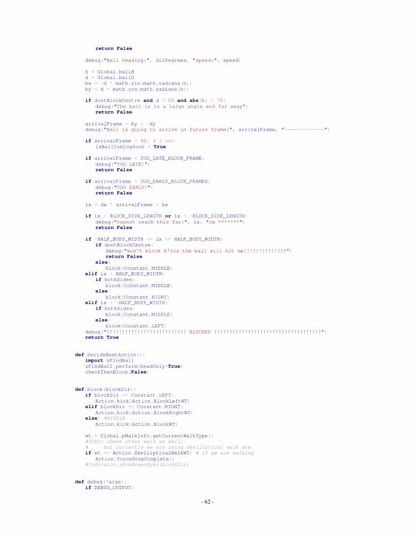
Appendix C
Source code of sBlock.py: import math import Global import Action import Constant import hTrack import Indicator import VisionLink #USAGE: (for external use) # call checkThenBlock() in appropriate place isBallComingSoon = False DEBUG_OUTPUT = False BLOCK_SIDE_LENGTH = 30 HALF_BODY_WIDTH = 18 / 2.0 TOO_LATE_BLOCK_FRAME = 0.1 * 30 TOO_EARLY_BLOCK_FRAMES = 0.9 * 30 # Check whether the robot should block the ball, and does so if yes. # If onlyVisualBall then a block will only trigger when the ball is # seen this frame. If the ball is moving slower than minBallSpeed then # this won't block. If the ball is nearer than minDist or farther than # maxDist it won't block. If bothSides is true then it will always block # both sides at once, else it may choose to block only one side. # Returns true if it blocks. def checkThenBlock(onlyVisualBall = True, minBallSpeed = 0.4, minDist = 30, maxDist = 80, bothSides = False, dontBlockCentre = False): global isBallComingSoon isBallComingSoon = False if onlyVisualBall and not hTrack.canSeeBall(): #debug("I can't see the ball!!") return False if Global.lostBall > Constant.LOST_BALL_LAST_VISUAL - 1: #if > 3 #debug("I have lost the ball >_<~~") return False if Global.ballD > maxDist: #debug("ball is too far away") return False if Global.ballD < minDist: #debug("ball is too close") return False _, _, speed, dirDegrees, _, _ = VisionLink.getGPSBallVInfo(Constant.CTLocal) if speed > 10: debug("Ball moves too fast, possible due to wrong ball") return False if speed < minBallSpeed: debug("Ball moves too slow, possible still ball with noise") return False dx = speed * math.cos(math.radians(dirDegrees)) dy = speed * math.sin(math.radians(dirDegrees)) if dy > 0: #debug("Ball is moving Away!")
- 62 -
return False debug("Ball heading:", dirDegrees, "speed:", speed) h = Global.ballH d = Global.ballD bx = -d * math.sin(math.radians(h)) by = d * math.cos(math.radians(h)) if dontBlockCentre and d > 50 and abs(h) > 70: debug("The ball is in a large angle and far away") return False arrivalFrame = by / -dy debug("Ball is going to arrive in future frame:", arrivalFrame, "-------------") if arrivalFrame < 90: # 3 sec isBallComingSoon = True if arrivalFrame < TOO_LATE_BLOCK_FRAME: debug("TOO LATE!") return False if arrivalFrame > TOO_EARLY_BLOCK_FRAMES: debug("TOO EARLY!") return False ix = dx * arrivalFrame + bx if ix > BLOCK_SIDE_LENGTH or ix < -BLOCK_SIDE_LENGTH: debug("cannot reach this far:", ix, "cm *******") return False if -HALF_BODY_WIDTH <= ix <= HALF_BODY_WIDTH: if dontBlockCentre: debug("won't block b'coz the ball will hit me!!!!!!!!!!!!!!") return False else: block(Constant.MIDDLE) elif ix > HALF_BODY_WIDTH: if bothSides: block(Constant.MIDDLE) else: block(Constant.RIGHT) elif ix < -HALF_BODY_WIDTH: if bothSides: block(Constant.MIDDLE) else: block(Constant.LEFT) debug("!!!!!!!!!!!!!!!!!!!!!!!!!! BLOCKED !!!!!!!!!!!!!!!!!!!!!!!!!!!!!!!!!!!") return True def DecideNextAction(): import sFindBall sFindBall.perform(headOnly=True) checkThenBlock(False) def block(blockDir): if blockDir == Constant.LEFT: Action.kick(Action.BlockLeftWT) elif blockDir == Constant.RIGHT: Action.kick(Action.BlockRightWT) else: #MIDDLE Action.kick(Action.BlockWT) wt = Global.pWalkInfo.getCurrentWalkType() #TODO: check other walk as well, # but currently we are using skelliptical walk atm if wt == Action.SkellipticalWalkWT: # if we are walking Action.forceStepComplete() #Indicator.showGreenEyes(blockDir) def debug(*args): if DEBUG_OUTPUT:

- 63 -
print __name__, for a in args: print a, print

- 64 -
Bibliography
1 Chi Kin Chan. Thesis B Report of RoboCup 2004
2 Alex North. Object recognition from sub-sampling image processing
3 Min Sub Kim, William Uther. Automatic Gait Optimisation for Quadruped Robots, 2003
4 Kim Cuong Pham. COMP3902 Special Project B Report
5 Nate Kohl and Peter Stone. Machine Learning for Fast Quadrupedal Locomotion, In The
Nineteenth National Conference on Artificial Intelligence, pp. 611–616, 2004
6 The German Team. RoboCup 2004 Report, 2004
7 Michael J. Quinlan, Craig L. Murch, Richard H. Middleton, and Stephan K. Chalup. Traction
Monitoring for Collision Detection with Legged Robots, pp. 374 - 384, In: Daniel Polani,
Brett Browning, Andrea Bonarini, and Kazuo Yoshida. RoboCup 2003: Robot Soccer World Cup
VII, Lecture Notes in Computer Science 3020, Springer-Verlag, 2004