odv-online howto

1

ODV-online HowTo Reiner Schlitzer, Alfred Wegener Institute, Bremerhaven, GERMANY ([email protected])

This document contains hands-on procedures for creating different kinds of graphics and products with ODV-online. The actual steps to be taken are highlighted in red boxes below.

If you are new to ODV-online (or the desktop ODV software) please familiarize yourself with the elements of the interface and the crucial role of mouse positioning as well as left and right mouse clicking. If you have used ODV before, you can skip this part and proceed directly to the first example.

ODV-online Primer

User Interface

Interactivity

As in the desktop ODV, left-clicking on station and sample locations selects the respective station or sample, while right-clicking on elements provides context menus with options for the manipulation of the clicked element.

Metadata of the current station, data of the current sample, and isosurface values for the current station are shown in the list windows on the right.

Interactive zooming, Z-zooming and point getter operations work by dragging the active edges or corners of the zoom boxes and by left-clicking a sequence of points. To terminate zoom and point getter operations, you click the Apply or Cancel buttons in the status bar or press the Enter or ESC keyboard keys.

mailto:[email protected]

2

Clickable metadata, data or info values, such as links to cruise reports, info files or other types of documents, are opened in a separate browser tab. You return to your ODV-online session by clicking on the respective browser tab.

Tooltips

Popup boxes showing more detailed information appear automatically if you rest the mouse over the ODV icon, the collection name in the title bar or over a variable name in the lists on the right side of the window.

Views

All data collections come with sets of prepared views on the data. Activating one of these views via View > Load View is the easiest way to get started with the exploration of the data in the collection. You can modify the view and save the modifications via View > Save View As and specifying a descriptive name, e.g., Oxygen_at_500m. Modified views are saved on your computer as part of your browser’s data and will exist until you clear the browser data. If you are using ODV-online after login (e.g., as a named user), your modified views are saved on our server and will persist, even after clearing your browser data.

Saved views appear as private views in the Load View trees. These views are invisible to other users.

Image files

High-resolution image files of the entire canvas, a particular data window or the map are obtained by right-clicking on the white background or the particular window and choosing Save Canvas As (or Save Plot As or Save Map As). A file save dialog will open, which lets you choose target directory and file name of the image file on your computer.

Close

Choose View > Close Session or close the browser tab to close your Explore session. Your last view settings are automatically saved and will be restored when you return. A session is automatically terminated after 60 minutes of inactivity.

Browser support

ODV-online runs on Chrome, Firefox, Safari, Edge (v79 or higher) and other modern browsers on desktop computers, laptops, tablets or smartphones. Microsoft Internet Explorer is not supported.

Further reading

In-depth information about Ocean Data View can be found in the ODV User’s Guide and at https://odv.awi.de/documentation/.

https://odv.awi.de/fileadmin/user_upload/odv/misc/odvGuide.pdf

https://odv.awi.de/documentation/

3

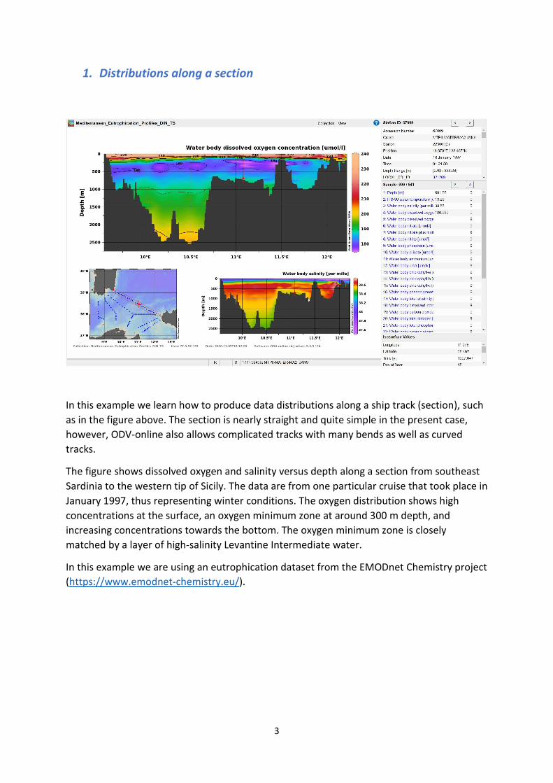
1. Distributions along a section

In this example we learn how to produce data distributions along a ship track (section), such as in the figure above. The section is nearly straight and quite simple in the present case, however, ODV-online also allows complicated tracks with many bends as well as curved tracks.

The figure shows dissolved oxygen and salinity versus depth along a section from southeast Sardinia to the western tip of Sicily. The data are from one particular cruise that took place in January 1997, thus representing winter conditions. The oxygen distribution shows high concentrations at the surface, an oxygen minimum zone at around 300 m depth, and increasing concentrations towards the bottom. The oxygen minimum zone is closely matched by a layer of high-salinity Levantine Intermediate water.

In this example we are using an eutrophication dataset from the EMODnet Chemistry project (https://www.emodnet-chemistry.eu/).

https://www.emodnet-chemistry.eu/

4

Open the dataset

Select cruise MTPII-MATER/MA2 JAN9

Define the section

Establish the window layout

In your webbrowser visit https://emodnet-chemistry.webodv.awi.de/, choose eutrophication > Mediterranean > Mediterranean_Eutrophication_Profiles_DIN_TS.odv. On the next page click DATA EXPLORATION.

Choose View > Load View and select public > Default.

Choose View > Layout Templates > 2 SECTION Windows. Right-click into the upper data window, choose Z-Variable and select 4: Water body dissolved oxygen… Then right-click into the lower data window, choose Z-Variable and select 3: Water body salinity.

Right-click into the map and choose Station Filter; visit the Name / Range page. In the Cruise label field enter MTPII-MATER/MA2 JAN9 or choose this entry from the list, then click Apply.

Zoom into the region between south Sardinia and western Sicily by right-clicking into the map, then choose Zoom. Drag the edges or corners of the zoom rectangle to the desired region and finally click the Apply button in the status bar.

Right-click into the map and choose Manage Section > Define Section, note that the cursor changed to cross-hair. Move the cursor to the north-western end of the northern section and left-click the mouse. Follow the track towards south-east and left-click again, repeat this 3 or 4 times until you reach the south-east end of the section and finally click the Apply button in the status bar.

On the Section Properties dialog choose Longitude as Section Coordinate and 20 km as Mean Width. Then click Apply. Note the section band appearing in the map.

https://emodnet-chemistry.webodv.awi.de/

5

Refine the data display

Save the current layout as named view by choosing View > Save View As and specifying a descriptive name, e.g., MTPII-MATER-MA2_JAN9. Obtain a high-resolution image of the entire canvas by right-clicking on the canvas (white background area) and choosing Save Canvas As.

Establish DIVA gridding by right-clicking into the upper data window and choosing Properties. Visit the Display Style page and in the combo-box under Gridded field choose DIVA gridding. Uncheck the Automatic scale lengths box, and for X and Y scale-lengths set 40 and 20, respectively. Uncheck the Draw marks box. Visit the Contours page. Set the Start, Increment and End values to 180, 10 and 270 and press the << button. Visit the Data page and press the Colorbar Settings button. Select (automatic) for Color mapping. Press Apply twice. Right-click again, choose Set Ranges and set the minimum oxygen value to 170.

Adjust the lower data window as described above.

6

2. Distributions on constant depth surface

In this example we learn how to produce data distributions on constant depth surfaces, such as in the figure above. Obtaining distributions on constant density surfaces (isopycnals) is very similar, but instead of depth a derived density variable is used to define the surface. You also learn how to use special map projections, such as oblique orthographic.

The figure shows dissolved oxygen at a depth of 500 meters in the subpolar North Atlantic and the Nordic Seas. Clearly visible are high oxygen levels in the Greenland and Irminger Seas indicating intensive vertical ventilation. Oxygen concentrations are much lower in the region south of Iceland and in the Norwegian Sea due to the influence of the North Atlantic Current carrying oxygen deprived waters northward into the Greenland Sea and Arctic Ocean.



7

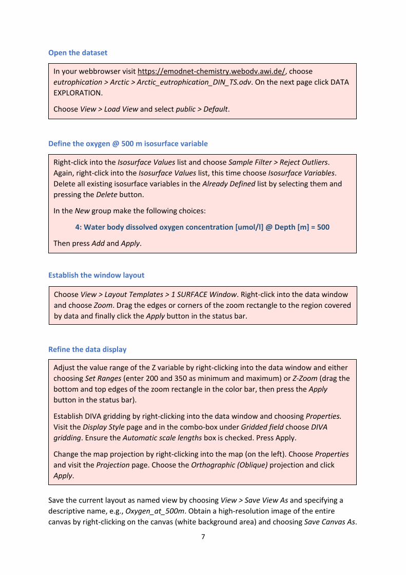
Open the dataset

Define the oxygen @ 500 m isosurface variable



Save the current layout as named view by choosing View > Save View As and specifying a descriptive name, e.g., Oxygen_at_500m. Obtain a high-resolution image of the entire canvas by right-clicking on the canvas (white background area) and choosing Save Canvas As.

In your webbrowser visit https://emodnet-chemistry.webodv.awi.de/, choose eutrophication > Arctic > Arctic_eutrophication_DIN_TS.odv. On the next page click DATA EXPLORATION.


Choose View > Layout Templates > 1 SURFACE Window. Right-click into the data window and choose Zoom. Drag the edges or corners of the zoom rectangle to the region covered by data and finally click the Apply button in the status bar.

Right-click into the Isosurface Values list and choose Sample Filter > Reject Outliers. Again, right-click into the Isosurface Values list, this time choose Isosurface Variables. Delete all existing isosurface variables in the Already Defined list by selecting them and pressing the Delete button.

In the New group make the following choices:

4: Water body dissolved oxygen concentration [umol/l] @ Depth [m] = 500

Then press Add and Apply.

Adjust the value range of the Z variable by right-clicking into the data window and either choosing Set Ranges (enter 200 and 350 as minimum and maximum) or Z-Zoom (drag the bottom and top edges of the zoom rectangle in the color bar, then press the Apply button in the status bar).

Establish DIVA gridding by right-clicking into the data window and choosing Properties. Visit the Display Style page and in the combo-box under Gridded field choose DIVA gridding. Ensure the Automatic scale lengths box is checked. Press Apply.

Change the map projection by right-clicking into the map (on the left). Choose Properties and visit the Projection page. Choose the Orthographic (Oblique) projection and click Apply.


8

3. Along-track distributions from profiling floats

In this example we learn how to produce data distributions along the track of drifting profiling floats, such as in the figure above. The procedure can also be applied to create similar temporal evolution plots from sets of hydrographic stations repeated over time in a small geographical region.

The figure shows chlorophyll-a data from a profiling float in the eastern Mediterranean over a two year period from 2013 until 2015. The track of the float is shown in the small plot on the lower right, colors indicating time. Evidently, the float is trapped in two eddies at the start of the observations (magenta/blue), before starting an eastward journey along the coast of Egypt (orange/red). The large plot at the top shows chlorophyll-a concentrations in the upper 380 m of the water column (Y axis) versus time (X-axis). Clearly visible are subsurface Chlorophyll maxima at around 100 m depth during most of the year, except for winter and spring times, when high chlorophyll concentrations reach up to the surface. Satellite sensors that can only “see” the upper ten meters of the water column are missing most of the chlorophyll signal.



9

Open the dataset

Select float PF_6901528

Define derived variables


Select X, Y, Z variables

In your webbrowser visit https://emodnet-chemistry.webodv.awi.de/, choose eutrophication > Mediterranean > Mediterranean_Eutrophication_Profiles_DIN_TS.odv. On the next page click DATA EXPLORATION.


Choose View > Derived Variables. Under Choices open the Metadata group, click on Latitude, then Longitude. Now open the Time group, and click on Time (station date/time). Click the Apply button.

Choose View > Layout Templates > 2 SCATTER Windows. Keep the station map untouched, but change the geometry of the two data windows one by one like in the figure above. Perform the following steps: right-click into the data window, choose Layout > Move / Resize Window, then drag the zoom rectangle to the desired location and size, and click the Apply button in the status bar. Make sure to leave margins on all sides of the data windows for color bar and axis annotations.

Right-click into the lower-right data window, choose X-Variable and select Longitude (near the end of the list). In the same way define the Y and Z variables as Latitude and Time (station Date/time), respectively. In the upper data window put Time (station Date/time) on X, and Water body chlorophyll (variable 13) on Z.

Right-click into the map and choose Station Filter; visit the Name / Range page. In the Cruise label field enter PF_6901528, then click Apply.

Zoom into the region of the drifting float by right-clicking into the map, then choose Zoom. Drag the edges or corners of the zoom rectangle to the desired region and finally click the Apply button in the status bar.


10


Save the current layout as named view by choosing View > Save View As and specifying a descriptive name, e.g., PL_6901528_Chl-a_along_track. Obtain a high-resolution image of the entire canvas by right-clicking on the canvas (white background area) and choosing Save Canvas As.

• Small data window: Increase the dot size by right-clicking into the data window, choose Properties and visit the Display Style page. Under Original Data choose a larger Symbol size. Press Apply.

• Large data window: Zoom into the upper water column by right-clicking into the data window, choose Zoom and drag the lower edge to a depth of about 380 m. Also move the left and right edges closer to the first and last data. Then click the Apply button in the status bar.

• Large data window: Establish DIVA gridding with contour lines. Right-click into the data window, choose Properties and visit the Display Style page. In the combo-box under Gridded field choose DIVA gridding and ensure the Automatic scale lengths box is checked. Uncheck the Draw marks box to switch off marking the data locations. Now visit the Contours page and simply click the << auto-create button. Remove all contour lines from the Already Defined list except the 0.05, 0.1, 0.2, and 0.5 lines by selecting the others and pressing the >> button. Press Apply.

odv-online howto

Documents